1

Microsoft Excel Part I Agenda:

1. Navigating through Workbooks and Worksheets and Menus 2. Data Entry 3. Basic Data Formatting 4. Sorting & Filtering Data

Data Entry To start the Excel spreadsheet software, double-click on the Excel icon.

You will then be presented with a blank worksheet like the one below.

*Remember, you must click on a cell before editing or formatting its contents. General rule with Microsoft Office programs – first select/highlight, then apply changes or formatting.

Formula Bar The ACTIVE CELL has a

bold outline.

These tabs show you

which sheet you are in.

2

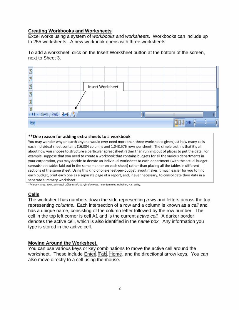
Creating Workbooks and Worksheets Excel works using a system of workbooks and worksheets. Workbooks can include up to 255 worksheets. A new workbook opens with three worksheets. To add a worksheet, click on the Insert Worksheet button at the bottom of the screen, next to Sheet 3.

**One reason for adding extra sheets to a workbook You may wonder why on earth anyone would ever need more than three worksheets given just how many cells each individual sheet contains (16,384 columns and 1,048,576 rows per sheet). The simple truth is that it’s all about how you choose to structure a particular spreadsheet rather than running out of places to put the data. For example, suppose that you need to create a workbook that contains budgets for all the various departments in your corporation, you may decide to devote an individual worksheet to each department (with the actual budget spreadsheet tables laid out in the same manner on each sheet) rather than placing all the tables in different sections of the same sheet. Using this kind of one-sheet-per-budget layout makes it much easier for you to find each budget, print each one as a separate page of a report, and, if ever necessary, to consolidate their data in a separate summary worksheet. **Harvey, Greg. 2007. Microsoft Office Excel 2007 for dummies. --For dummies. Hoboken, N.J.: Wiley.

Cells The worksheet has numbers down the side representing rows and letters across the top representing columns. Each intersection of a row and a column is known as a cell and has a unique name, consisting of the column letter followed by the row number. The cell in the top left corner is cell A1 and is the current active cell. A darker border denotes the active cell, which is also identified in the name box. Any information you type is stored in the active cell. Moving Around the Worksheet. You can use various keys or key combinations to move the active cell around the

worksheet. These include Enter, Tab, Home, and the directional arrow keys. You can

also move directly to a cell using the mouse.

Insert Worksheet

3

Exercise: Practice entering data into different cells. Try entering your first name, last name, address, town, state, email, etc. Try moving around the worksheet using various keys.

**Reference Table: Moving the Cell Cursor** Keystroke Where the cell cursor moves

or Tab Cell to the immediate right

or Tab Cell to the immediate left Cell up one row Cell down one row

Home Cell in Column A of the current row

Ctrl + Home First cell (A1) of the worksheet

Ctrl + End or End, Home Cell in the worksheet at the intersection of the last column that has any data in it and the laws row that has any data in it (that is, the last cell of the so-called active area of the worksheet)

PgUp Cell one full screen up in the same column

PgDn Cell one full screen down in the same column

Ctrl + or End,

First occupied cell to the right in the same row that is either preceded or followed by a blank cell. If no cell is occupied, the pointer goes to the cell at the very end of the row.

Ctrl + or End,

First occupied cell to the left in the same row that is either preceded or followed by a blank cell. If no cell is occupied, the pointer goes to the cell at the very beginning of the row.

Ctrl + or End,

First occupied cell above in the same column that is either preceded or followed by a blank cell. If no cell is occupied, the pointer goes to the cell at the very top of the column.

Ctrl + PgDn Last occupied cell in the next worksheet of that workbook.

Ctrl + PgUp Last occupied cell in the previous worksheet of that workbook.

**Harvey, Greg. 2007. Microsoft Office Excel 2007 for dummies. --For dummies. Hoboken, N.J.: Wiley.

Correcting Data Entry Errors To delete the entire contents of a cell, click on the cell, then press the delete key on the keyboard. To correct a typo, double-click on the cell, and a cursor will appear. You can then use the backspace or delete keys to make corrections. Another way to correct a typo is to click on the cell you are editing. Then click on the formula bar to edit the cell’s contents. Exercise: Delete the data that you entered into the spreadsheet. The Formula Bar The Formula Bar is directly above the worksheet. You can enter data for each active cell in the formula bar or in the cell itself. Notice that the Formula Bar mirrors the contents of the active cell.

4

A note about letting the contents of a cell overflow into the next cell: Don’t do it! Instead, resize your columns. Autofill You can use Autofill to copy text throughout a range of cells. Position the mouse

pointer on the lower-right corner of the cell you wish to copy, and the Autofill Handle + will appear. Drag the mouse pointer through the cells you want to fill in.

Exercise: Type “Barrington” in cell C1 and use Autofill to copy the text in cells C2 through C6. Then type “January” in cell D1 and use Autofill to complete cells D2 through D6. Notice that Excel automatically completes the sequence of months. Use the Autofill drop-down menu to select “copy cells” or “fill series.”

Inserting Blank Columns and Rows Simple commands allow you to delete rows and columns or insert rows and columns anywhere in the worksheet.

Autofill drop-down

menu

5

From the Home tab, click on the Insert or Delete drop-down menu, then select rows or columns. Excel always inserts a new row or column directly before the active cell, i.e. to the left of the selected column or above the selected row. Exercise: Open the saved workbook on your computer titled: “Excel Basics Address List.” Add a new column before Column G (Client). Type “Country” in call G1. In cell G2, type “USA.” Use Autofill to complete the column. Insert a new row above Row 1. Type “Address List” in cell A1. Formatting Data Changing Column and Row Width/Height Sometimes rows and columns are not large enough to accommodate your data. You can adjust the height and width of rows and columns individually, or you can adjust all rows and columns at once. To adjust a single column or row, place the mouse pointer on the boundary of the column or row heading. It will turn into a cross with two directional arrows. Drag the mouse to expand or contract the row or column, then release the mouse. Double-click on the column’s boundary line to automatically size the column to fit its contents. To make all of your rows or columns a uniform size, highlight the entire worksheet by clicking in the top left corner below the name box. Then resize any one row or column.

Insert

Delete

Position mouse pointer

here to re-size column

Position mouse pointer

here to re-size row

6

Shrinking Text Another option is to shrink the text to fit the existing column width. Select the cell in question, click on the arrow next to Alignment, choose Shrink to Fit, and click OK.

Merge and Center The Merge and Center function allows you to center text across several cells and is useful for adding titles or section headings to your worksheet. Exercise: Highlight cells 1A-1G. Click the Merge and Center button to center “Address List” across the top of the spreadsheet. Borders The dividing lines between cells will not appear on a printed page unless you draw them in. Exercise: Highlight the portion of the sheet that contains data. Click on the pull-down arrow of the Borders button on the Ribbon. Select All Borders. Other Formatting Tools You can use the Bold, Italics, Underline, and Text Alignment buttons on the Ribbon to apply formatting to a single cell, row, column, or the entire worksheet. Highlight the portion of the sheet you wish to format, then click on the appropriate button on the Ribbon.

Alignment

Merge and Center

Borders

7

Printing To see how your worksheet will look on a printed page, click on the Office Button, select Print, then Print Preview. Notice that what you see on the computer screen is not necessarily what will appear on the printed page.

You can also use the Page Layout view to see how your spreadsheet will look when printed. You can format your data here and see how the changes look. You can flip back and forth between the Page Layout and Normal view in the “View” tab.

8

Fitting Text to Your Page If your worksheet does not fit on the page, try changing the page Orientation from Portrait to Landscape. Alternatively, try using Scale to Fit. This function will shrink the size of your printed text to fit on the page. Both options are in the Page Layout tab of the Ribbon.

You can also use the Page Break Preview function to view your spreadsheet and the printed page contents. Click/hold/drag the blue border outlines to change what fits on a page.

Sorting Data Single Level Sorting Exercise: Click on any cell in the Last Name column (except the header row), then click on the Sort & Filter button on the Ribbon. Select Sort A to Z. The list is now alphabetical by last name. To reverse the sorting order, select Sort Z to A.

Orientation

Scale to Fit

9

Multiple Level Sorting To sort by multiple criteria, select Custom Sort from the Sort & Filter Button.

Use the drop-down menus to select which column to sort and in what order. Click Add Level to include secondary or tertiary criteria to the sort order. Select the box indicating “My data has headers” to keep the column labels in place.

10

Filtering To turn on the AutoFilter, click a cell in the table you want to filter, and choose the Filter button under Sort & Filter on the Data tab. Gray filter arrows appear on each column heading. Click on these arrows to filter data by column. Multiple filters can be set. When you’re done filtering – or at any time you want to remove filters - turn AutoFilter off by clicking the Filter button again.

11

Final Exercise Recreate the worksheet below.

Exiting Excel You can either:

- Click the Office Button followed by the Exit Excel button - Click the Close button in the upper-right corner of the Excel program window (the

red X box)