WORKING PAPER SERIESFED

ERAL

RES

ERVE

BAN

K of A

TLAN

TA

Microentrepreneurship and the Business Cycle: Is Self-Employment a Desired Outcome? Federico S. Mandelman and Gabriel V. Montes Rojas Working Paper 2007-15 July 2007

The authors thank Maria Laurel Graefe for superb research assistance and very useful suggestions. They also thank Pablo Acosta, Julie Hotchkiss, and Lucas Siga for very helpful comments. The views expressed here are the authors’ and not necessarily those of the Federal Reserve Bank of Atlanta or the Federal Reserve System. Any remaining errors are the authors’ responsibility. Please address questions regarding content to Federico Mandelman, Research Department, Federal Reserve Bank of Atlanta, 1000 Peachtree Street, N.E., Atlanta, GA 30309-4470, 404-498-8785, federico.mandelman@ atl.frb.org; or Gabriel Montes Rojas, the University of Illinois at Urbana-Champaign, 1206 South Sixth Street, 484 Wohlers Hall, Champaign, IL 61820, rmontes@uiuc.edu. Federal Reserve Bank of Atlanta working papers, including revised versions, are available on the Atlanta Fed’s Web site at www.frbatlanta.org. Click “Publications” and then “Working Papers.” Use the WebScriber Service (at www.frbatlanta.org) to receive e-mail notifications about new papers.

FEDERAL RESERVE BANK of ATLANTA WORKING PAPER SERIES

Microentrepreneurship and the Business Cycle: Is Self-Employment a Desired Outcome? Federico S. Mandelman and Gabriel V. Montes Rojas Working Paper 2007-15 July 2007 Abstract: This paper links employment dynamics to the business cycle in order to examine the voluntary nature of self-employment in Argentina. Our results suggest that the transition to self-employment is more common during recessions and that the likelihood of becoming self-employed increases with the length of the recession and the unemployment duration. We find that the majority of self-employed workers do not have employees and earn significantly less than salaried workers. Individuals in this sector are often young and less educated and have trouble obtaining a salaried position regardless of the macroeconomic conditions. Middle-aged, college-educated individuals also tend to enter self-employment as a temporary refuge when they encounter difficulties during a recession. Our results suggest, however, that for entrepreneurs who have employees, entry into self-employment is procyclical and voluntary and has characteristics similar to those predicted for highly skilled risk-taking entrepreneurs. Including idiosyncratic entrepreneurial abilities in a standard job search model allows us to predict such labor market segmentation and the cyclical pattern of entrance into self-employment. JEL classification: J23, L25, E32 Key words: microfirms, self-employment, business cycles

Microentrepreneurship and the Business Cycle: Is “Self-Employment”a Desired Outcome?

1 Introduction

Mounted on the success of the Silicon Valley high-tech start-ups, the view of self-employment in in-

dustrialized countries is remarkably positive. Self-employed workers are generally regarded as creative

and high qualified individuals who have abandoned the comfort of salaried positions to invent new

products, production process and distribution methods. The sector is dynamic and populated by “su-

perstars” that obtain outstanding profits and social influence, bringing vitality to the economy and

decisively contributing to its expansion.1 In response to this view, many countries have been devel-

oping supportive policies to stimulate these self-started projects.2 Such optimism finds support in the

bulk of the theoretical literature and empirical evidence on the matter.3 Although some studies show

that small business owners register lower median earnings growth than those in paid employment, such

gap is not considered to be the result of low-ability selection bias, rather the result of non-pecuniary

benefits, such as “being your own boss.”4 To sum up, a growing strand of the literature considers

self-employment an optimal and voluntary decision.

Interestingly, we observe that the same conclusions are being attached to the microenterprise sector

in the developing world, where it comprises a large fraction of the working population. Despite the

scarcity of studies in this region, an emerging perspective in the academic literature stresses the micro-

entrepreneurial dynamism, voluntary entry and job satisfaction. In broad terms, these studies attempt

to show that microenterprises in emerging economies (particularly in middle-income countries) show

1Rosen (1981) discusses the “superstar” theory.2 See Blanchflower and Oswald (1998).3For a survey on the literature see Blanchflower (2004). Classic contributions include: Lucas (1978), where individuals

are endowed with a given and known entrepreneurial ability. Those with a sufficiently high level of managerial abilitybecome entrepreneurs, while the rest become wage workers. Jovanovic (1982) adds dynamic and uncertainty about theseskills. Evans (1987) describes industrial dynamics that permit a characterization of microfirms. Rees and Sha (1986)argue that more educated individuals have a lower cost of assessing business opportunities and that human capital is acomplement to managerial abilities.

4 See Hamilton (2000).

1

dynamic patterns consistent with the entrepreneurial risk-taking framework in the industrial world.5

They conclude that such strong similarities suggest that mainstream models could be useful guides for

policymaking in the existing developing-country microenterprise sector.6

To put it bluntly, the objective of this paper is to answer a key question that would guide policy-

makers: Is the above description an appropriate characterization of self-employment, or is it more

accurately explained by the traditional economic development literature that views this sector as being

stagnant, serving merely as a refuge of last resort for the urban unemployed?7Given that resources are

scarce, governments and multilateral organizations may face a trade-off between devoting resources to

support entrepreneurial activities or spending them elsewhere, for instance, to promote education and

training.

We analyze the labor market in Argentina, a middle-income country that has a sizeable self-

employment sector, and track individuals in the period 1995-2003. Our comprehensive data set is

unique in the sense that contains a rotating household panel survey that is suitable to perform a

comparison with firm dynamics in developed economies. The study relies on probit and multinomial

logistic models. In addition, we propose an innovative approach that links employment transition

dynamics vis-à-vis to the business cycle. It is important to mention that during such a short period

of time, the economy witnessed a remarkable variety of macroeconomic scenarios: Namely, a short-

lived recession, a two-year period of extraordinarily high economic growth, a long-lasting economic

depression followed by a dramatic economic crisis, and a recovery. This sizable business cycle is used

to judge the voluntary nature of employment transitions in terms of what have been called the “push”

and “pull” factors of the labor supply. To characterize the “push” factors, consider a depressive

context with high unemployment levels and no business opportunities; such scenario allows us to link

self-employment transitions to employment of last resort or disguised unemployment. To the contrary,

“pull” factors play a role when macroeconomic conditions are good. The prospects for business are

5This literature have roots in Hart (1972). Examples include: De Soto (1989), Maloney (1999, 2004), Battacharya(2002), Fajnzylber et al (2006) and Ñopo and Valenzuela (2007).

6 See Fajnzylber et al (2006).7These views have roots in Harris and Torado (1970). The labor market is segmented by wage settings in the formal

sector that leaves the urban unemployed rationed out of the modern salaried employment, forcing them to remaininformal and search for a refuge in the self-employment sector. Rauch (1991) model endogenously determines the choicebetween formal and informal sector.

2

better and qualified individuals with entrepreneurial abilities may voluntarily choose to become self-

employed, knowing that if the venture fails another job offer will not be far away.8 We argue that

this “revealed” evidence is more appropriate than surveys that directly address the voluntary nature

of the transition. As shown in Blanchflower (2004), individuals tend to be unrealistically optimistic

when disclosing prospects about their own business projects.

In order to answer the questions posed above, we report the following key findings: (a) Conditional

on skill levels, self-employed workers earn on average 8.3 percent less than salaried workers and they

also have 1.9 percent less income growth.(b) Economic recessions are associated with a monotonic

increase in the amount of individuals (salaried and unemployed) that transition to self-employment.

However, this trend sharply reverts when the economy starts growing (the lowest transition point

is at the peak of the macroeconomic activity). (c) Recessions improve the performance of salaried

workers, putting into question the voluntary nature of such transition.9(d) Years of economic booms

are characterized by less educated individuals with few entrepreneurial skills becoming self-employed,

and more educated self-employed individuals becoming salaried workers. This trend reverts when the

recession begins. Therefore, when the economy is performing well, self-employment is only a profitable

alternative for those low educated individuals who are unable to find a job in the salaried sector. As

the recession hits, it expands the pool of workers looking for a job, and it increases the likelihood of

more educated individuals (particularly middle-age college educated individuals) starting their own

micro-businesses.(e) When the recession deepens, and average unemployment duration increases, the

proportion of unemployed workers that move to self-employment drastically rises. Besides, a successful

transition to a salaried position is less likely if the unemployment spell is long. (f) On average, workers

in larger firms and with higher salaries are less likely to start an entrepreneurial activity. A preliminary

conclusion is clear: self-employment is unlikely to be the result of an optimal and voluntary decision

taken by high-skilled individuals. Instead, it should be regarded as a refuge for the urban unemployed.

Earle and Sakova (2000) reject the pooling of own-account workers and self-employed individuals

that also have their own employees since their intrinsic characteristics are different. We find a striking

8For details and related literature see Carrasco (1999).9 Since the reverse cyclical conclusion does not apply, we discard that this fact is simply the result of nominal wage

rigidities.

3

segmentation when we take this distinction into account. Contrary to the general conclusions above,

results indicate that: (g) recessions are associated with a decline in the proportion of individuals

that become self-employed with employees. (h) The probability of becoming an entrepreneur with

employees monotonically increases in both education and age. (i) People that are currently employed

and with higher conditional salaries are more likely to transition into this category. In other words,

only when we focus in this category do we find patterns that are similar to the optimistic view discussed

above. The evidence supports the existence of experienced and talented individuals who were able to

accumulate enough capital and managerial abilities to start their own business projects and generate

employment. Nonetheless, this phenomenon is very limited in nature: Two-thirds of the self-employed

are actually own-account workers, and if they manage to survive, they will most likely remain within

this category. Moreover, the self-employment sector in developing countries is much larger than those

that exist in the developed world.

We show that the employment dynamics above may be captured by an extended job search model

that includes idiosyncratic entrepreneurial abilities and business cycle properties. This model leads

to a labor market that is clearly segmented. Those with extraordinary entrepreneurial abilities (pure

entrepreneurs), or the remarkably low-qualified individuals with little chance to find employment in

the job market (misfits) may choose to be self-employed on a permanent basis. Other workers may

face serious difficulties finding paid jobs during recessions and may regard self-employment as a safe

refuge while searching for a proper salaried position.

The rest of the paper is organized as follows: Section 2 presents the theoretical model. Section

3 shows descriptive statistics. Section 4 discusses the employment transition dynamics. The micro-

econometric analysis is presented in section 5. Concluding remarks are in section 6.

2 Model

In order to analyze employment transition and business cycle properties, we consider an extension

of the classic intertemporal job search model (McCall, 1970). The key contribution of our model is

the inclusion of idiosyncratic entrepreneurial abilities and business cycle properties that result in a

4

segmentation of the labor market.

Model Setup Consider an individual who is searching for a job. The model is stochastic, in

the sense that each period the worker draws, with no cost, one offer w(θi) from what she perceives

(with complete certainty) to be her idiosyncratic wage cumulative distribution F (W (θi)) = F θi =

prob w ≤W , with F θi(0) = 0, F θi(Ω) = 1 for Ω(θi) < ∞. Here θi captures intrinsic work ability

(human capital) and entrepreneurial skills for the individual under consideration.

Every period the worker has the option of rejecting the job offer, in which case she receives unem-

ployment compensation z(θi), such that Ω > z(θi) > 0, and waits until the next period to draw another

offer from F θi . We assume that the unemployed worker can not receive this temporary compensation

for more than τ consecutive periods. The individual may also become self-employed while searching

for a salaried position. In this case the individual gets c(θi) and no unemployment compensation. Of

course, at any time the individual can stop looking for a job and become self-employed on a permanent

basis with same compensation c(θi).10

Alternatively, the worker can accept the offer to work at w, in which case she receives a wage w per

period thereafter. During her “living” tenure neither quitting nor being fired is permitted. Nonetheless,

each period the worker faces a fixed probability of surviving α ∈ (0, 1) with her idiosyncratic status

θi. That is, the “death” of the individual should be interpreted as a change in her intrinsic ability.

For the sake of simplicity, we assume that individuals maximize only over their “living” tenure (as

in Sargent and Ljungqvist, 2000), and that the “death” shock occurs independently of the original

idiosyncratic status θi. After “dying”, the individual is “reborn” and draws a new θj status with a

new wage distribution F (W (θj)) = F θj , and thus proceed with a new reoptimization and job search.

Optimization Let yt be the worker’s income in period t. We find three possible scenarios: we

have that yt = w if the worker has accepted an offer to work at wage w. If the unemployment spell

is no longer than τ , and z(θi) > c(θi) the worker’s income is: yt = z(θi), otherwise she derives her

10 In c(θi), we may include non-pecuniary benefits, such as “being your own boss.”

5

income from self employment, yt = c(θi).11

The unemployed worker devises a strategy to maximize EΣ∞s=t(βα)s−tys. Where 0 < β < 1 is a

discount factor adjusted for her survival rate α. Let νθi(w) be the expected value of EΣ∞s=t(βα)

s−tys,

for a worker who has an offer w in hand, who is deciding whether to accept or reject it and behaves

optimally. At period t, the Bellman equation for the worker’s problem is:

νθi(w) = max

(w

1− βα, z(θi) + βα

Z Ω(θi)0

νθi(w0)dF θi(w0),

c(θi)

1− βα

)if t 6 τ and z(θi) > c(θi).

(1)

and,

νθi(w) = max

(w

1− βα, c(θi) + βα

Z Ω(θi)0

νθi(w0)dF θi(w0),

c(θi)

1− βα

)otherwise. (2)

Where the maximization is over three options: (1) accept the wage offer w and work at wage w

during the living tenure; (2) reject the offer and draw a new offer w0 from distribution F θi . In the

meantime, receiving either unemployment compensation, z(θi), or being temporarily self-employed

and earning c(θi); (3) or becoming permanently self-employed and receiving c(θi). The solution will

be of the form:

νθi(w) =

⎧⎪⎪⎪⎪⎨⎪⎪⎪⎪⎩I(θi) + βα

R Ω(θi)0

νθi(w0)dF θi(w0) if w 6 w(θi)

w(θi)1−βα if w > w(θi)

c(θi)1−βα if c(θi) > Ω(θi)

⎫⎪⎪⎪⎪⎬⎪⎪⎪⎪⎭ (3)

Where w(θi) is the reservation wage and I(θi) is a function that takes the value z(θi) if t 6 τ

and z(θi) > c(θi), and c(θi) otherwise. Since the individual can draw a new offer at no cost, and

11The standard search model assumes that leisure does not provide any utility to the individual. If z(θi) = c(θi), theunemployment and self-employment compensation are identical. We assume that in such scenario the individual prefersto remain unemployed.

6

always have the possibility of being self-employed while waiting for the right job, we easily deduce

that only those who earn a self-employment income, c(θi), higher than any other possible job offer

(i.e. c(θi) > Ω(θi)), will stop looking for a paid job and become permanently self-employed.

Let us now focus on those who search for a wage earning position. Using equation (3) we can

convert the functional equation (2) into an ordinary mapping, νθi(w), in the reservation wage w(θi).

Evaluating νθi(w), and using equation (3), we have:

(w(θi)− I(θi)) =βα

1− βα

Z Ω(θi)w

(w0 − w(θi))dFθi(w0) (4)

Equation (4) is used in the job search literature to characterize the determination of the reservation

wage w. The left side is the cost of searching one more time when an offer w is in hand. The right side

is the expected benefit of searching one more time in terms of the expected present value associated

with drawing w0 > w. Equation (4) informs the worker to set w so that the cost of searching one more

time equals the benefit. Define the function on the right side of equation (4) as:

u(w(θi)) =βα

1− βα

Z Ω(θi)w

(w0 − w(θi))dFθi(w0) (5)

Notice that u(0) = β/(1 − β)Ew(θi), that u(Ω(θi)) = 0, and that u(w(θi)) is differentiable with

derivatives12 given by:

u0(w(θi)) = − βα

1− βα

£1− F θi

¤< 0 (6)

u00(w(θi)) =βα

1− βα(F θi)0 > 0 (7)

12We apply Leibniz’ rule to compute u0(w(θi)). Let Θ(ζ) =γ(ζ)δ(ζ)

f(x, ζ)dx for ζ [c, d]. Assume that f and ∂f∂ζ

are continuous and that γ, δ are differenctiable [c, d], then we get that: Θ0(ζ) = f [γ(ζ), ζ] γ0(ζ) − f [δ(ζ), ζ] δ0(ζ) +γ(ζ)δ(ζ)

∂f∂ζ(x, ζ)dx. Let w(θi) play the role of ζ when applying this formula.

7

So that u(w(θi)) is convex to the origin. Given the idiosyncratic work ability and entrepreneurial

skills, θi, we can graph u(w(θi)) against w(θi) to determine w(θi) and characterize the labor market

segmentation. Refer to Figure 1 for an example.

Business Cycle Properties To make matters interesting, we include a business cycle analysis in

this simple setup. We rely on the classic “misperception” business cycle theory in which the factor that

influences workers’ decision is the misperception of real wages (Lucas, 1973). For example, assume that

the general level of prices, including the level of nominal wages, increases as a result of an unexpected

monetary expansion. In principle, real variables should remain unaffected given the assumption that

money supply is neutral. However, workers mistakenly perceive the increment in nominal wages as

an increment in the real level of wages that are being offered in the job market. More jobs offers are

accepted, and therefore individuals work and produce more. Inverse results would follow a monetary

contraction (that in emerging economies could be the result of capital outflows).13

Consequently, in the boundaries of our simple setup, an economic expansion is a situation in which

actual wage draws are on average higher than the ones workers had expected to obtain. Now, let us say

that the actual idiosyncratic wage cumulative distribution is defined as follows: FA(W (θi)) = F θiA =

prob w ≤W , with F θiA (0) = 0, F

θiA (Ω

A) = 1 for ΩA(θi) <∞. In any period t, the misperception that

defines an economic expansion is such that: ΩA(θi) > Ω(θi), and F θiA < F θi , so that EA > Ew(θi).

Where Ew(θi) is the average wage offer expected by the individual and EA is the mean value of the

actual wage distribution. To the contrary, during an economic recession such misperception works in

the opposite direction: ΩA(θi) < Ω(θi), FθiA > F θi , with EA < Ew(θi).

Following this line of argument, we may distinguish a situation in which workers’ misperceptions are

more severe and thus the recession is deeper. If we define the wage distribution during a pronounced

recession as F θiA(deep), our argument implies that F

θiA(deep) > F θi

A > F θi with ΩA(deep)(θi) < ΩA(θi) <

Ω(θi). Figure 2 graphs this distinction. A reverse analysis can be used to characterize a booming

economy: F θiA(boom) < F θi

A < F θi with ΩA(boom)(θi) > ΩA(θi) > Ω(θi).

13There are alternative ways to model this misperception and get the same results. Assume, for instance, that eachworker obtains a wage offer with a given probability each period (See Mortensen, 1986, for details). If the worker believesthat in every period such probability is equal to λw; recessions (booms) are going to be characterized for a situation inwhich the actual probability of receiving an offer, λa, is such that, λa < λw (λa > λw).

8

2.1 Labor Market Segmentation

Given idiosyncratic ability and skills, this labor market characterization allows us to segment the

market in three different sectors: Salaried workers, Pure Entrepreneurs and Misfits.

Salaried Workers “Salaried Workers” are those individuals who are either employed (and re-

ceive wage compensation), or are looking for a permanent salaried position. Figure 1 indicates the

reservation wage w(θi) that satisfies (w(θi)− I(θi)) =βα1−βα

R Ω(θi)w

(w0 − w(θi))dFθi(w0) = u(w(θi)).

From this analysis we can derive some intuitive theoretical results. First, if the unemployment

compensation, z(θi), is smaller than the income the worker can derive from self-employment, c(θi),

the worker will regard self-employment as a “temporary refuge” while looking for paid employment

that satisfies her reservation wage.

Second, assume that the economy is in a recession and z(θi) > c(θi). In equation (3) we show

how the reservation wage, w(θi), is derived from the individual perceptions. We also know that a

recession is characterized by an idiosyncratic distribution in which actual wage draws are (on average)

lower than the workers’ expectations. Therefore, it is more likely for the worker to obtain draws that

are below her reservation wage (i.e. F θiA (w(θi)) > F θi(w(θi))); and consequently the search process

and unemployment duration are longer on average. To sum up, in aggregate terms, the number of

individuals who remain unemployed for more than τ consecutive periods and are forced to seek self-

employment as a temporary refuge (while searching for a salaried position) increases during recessions.

The deeper and longer the recession is, the larger the amount of individuals in this situation.

Pure Entrepreneurs “Pure Entrepreneurs” are highly qualified individuals with exceptional

entrepreneurial abilities who perceive that the income they may obtain from self-employment, c(θi) is

at least as high as any other possible wage offer they may obtain in the job market (i.e. c(θi) > Ω(θi)).

Although they may face attractive job offers, they never look for a salaried position.14 Refer to Figure

14This model might be easily extended to capture some other intuitive results. For instance, economic expansions areassociated with productivity innovations and technological improvements that result in new niches for profitable businessstartups. As a result, business entry is procyclical (see Bilbiie et al, 2006, for references). In our model terminology, wecould interpret that economic expansions are linked to periods in which the proportion of “newborns” z with exceptionalabilities (i.e. c(θz) > Ω(θz) ∀z) is higher.

9

3.

Misfits “Misfits” are individuals who are severely disadvantaged in the labor market, as for

example, young, inexperienced individuals with no formal education. Even though the income they

can earn from low-qualified self-employment, c(θi), is very low, they realize that job offers they could

get are negligible in value. As a result, the same condition (i.e. c(θi) > Ω(θi)) applies. Figure 4 plots

this category.

3 Descriptive Statistics and Employment Dynamics.

We use the Encuesta Permanente de Hogares (EPH), an urban household survey tracking individuals

for 2 years, both in May and August, from 1995 to 2003.15 The survey covers most Argentinean

metropolitan areas and is one of the most representative databases of urban employment available of

this frequency in Latin America. As usual, we only consider individuals in the age range 20-65, which

comprise the active labor force (in Argentina, retirement age is between 60 and 65, although slightly

lower for public employees).

Table 1 presents basic statistics for the pooled EPH sample. Some stylized facts emerge from

the table. On average 27 percent of the labor force is self-employed, which is a relatively large

number. For instance, self-employment compasses only 6 percent of the urban employment in the

United States.16 The individuals in this sector are relatively older and less educated than salaried

workers. We also observe a high dispersion and heavy tails, meaning that we encounter both very

unskilled and professionals in this category. Average income of the self-employed is 20 percent greater

than that of salaried workers. However, when controlling for observable skills, salaried workers earn on

average 8.3 percent more than self-employed.17 Entrepreneurs have an average annual hourly income

growth of -4.8 percent which contrast with -1.9 percent of salaried workers. This difference is also

15However, since we will be mostly interested in annual transition and income dynamics, our sample will be reducedto May 1995-May 2002.16 See Blanchflower (2004).17We run a regression where the dependent variable is the logarithm of hourly wage and we use a dummy variable for

salaried as an independent variable, controlling for years of schooling, age, gender, an indicator for household head, andyear and regional dummies. Regression coefficients are not reported but are available upon request.

10

robust to additional controls, showing an average income growth difference of 1.9 percent.18 Finally,

household heads and males are more likely to be self-employed.

Table 2 shows the distribution of workers in each sector by firm size. Notice that about two-thirds

of the self-employed are own-account workers. Table 3 presents the distribution of workers in each

sector by industry. In particular, we note that about 50 percent of the self-employed are in three main

sectors: retail trade, construction and repair services.

In order to have a sense of how many individuals change from one status to another, we compute

the dynamics of moving in or out the self-employment sector. In Table 4.a we present transition

dynamics from three sectors: self-employment, salaried and unemployment. For simplicity we exclude

individuals not in the labor force. We observe that about 71 percent of self-employed workers stay

in that sector, while roughly 20 percent go to (and come from) the salaried sector. The remaining

9 percent transit to (and from) unemployment. The salaried sector shows the least mobility among

the three sectors - around 85 percent of workers stay from one year to the next. Also note that self-

employed workers are 50 percent more likely to be unemployed one year later than salaried workers.

Finally, it is worth noting that of those workers who begin as unemployed, around 40 percent of them

is absorbed by the salaried sector, this is about twice as many individuals as the self-employed sector

absorbs. Nonetheless, if we acknowledge the relative size of each sector, the unemployed who move

to the salaried sector represent 6 percent of salaried workers while the unemployed absorbed by the

self-employed represent for 13 percent of self-employed. Table 4.b shows firm size dynamics for those

that start and end up as self-employed. The vast majority (around 82 percent) of the own-account

workers who manage to survive remain in this category and do not hire employees. Those who start

with at least with one employee most likely remain with employees. The more employees the firm

posseses, the lower the possibility the employer has of becoming an own-account worker. Similarly,

the likelihood of hiring additional employees is monotonically related with the size of the firm. For

instance only 4.9 percent of firms with 1 to 4 employees expand, while 21.5 percent of firms with 15

to 24 employees move to the category that comprises firms with more than 25 employees.

18Here the dependent variable is the annual hourly income growth rate, and we use the same controls as before.Regression coefficients are not reported but are available on request.

11

4 Business Cycle and Transition Dynamics

Figure 5 reports the evolution of real gross domestic product (GDP) and unemployment rate in Ar-

gentina for the years 1994-2003. Although this is a short period of time, the variety of macroeconomic

scenarios and the size of the business cycle contribute to make this study more appealing. The Mexican

economic crisis is to certain extent inherited by Argentina (process known as the Tequila effect), and

the economy witnesses a short-lived recession during 1995. Thereafter, the economy recovers strongly

until 1998 (GDP growth of 8 percent in 1997). Following the successive negative shocks from East

Asia, Russia and Brazil; Argentina enters into a long-lasting recession at the end of 1998 (with GDP

falling 3 percent). Meanwhile, the issue of Argentina’s massive public debt becomes a subject of

considerable controversy, capital outflight increases, and soon the government finds itself unable to

meet debt payments. The chaotic crisis explodes after an almost complete freezing of bank deposits

at the end of 2001. In 2002, Argentina’s GDP sinks by 10.9 percent with respect to the previous year.

The economy finally recuperates in 2003. Unemployment falls when the Tequila effect is over, but

significantly increases during the four-year recession that follows. The crash of the economy in 2001

brings a clear spike in the jobless rate.

Figure 6 depicts the evolution of hourly wages for the period 1995-2003 both in levels and in annual

differences (left scale and right scale respectively). The figure shows a context of deterioration of real

wages and a 30 percent fall in average hourly wages in the aftermath of the 2001 economic crisis. The

evolution of total self-employment and own-account rates as a proportion of the total active labor force

is shown in Figure 7. First, notice that total self-employment significantly increases after the Tequila

effect. Thereafter, own-account employment participation in total self-employment is countercyclical.

When the economy expands, overall self-employment increases, but the own-account sector is almost

non-reactive. The situation changes when the recession begins in 1998. During this period, the growth

rate of own-account employment surpasses the growth rate of aggregate self-employment, and the

growth rate gap continues to increase in the aftermath of the economic crisis.

Figure 8 represents the evolution of the salaried premium in levels (obtained as in the previous

subsection) over the period of analysis. Here we also distinguish between own-account workers and

12

self-employed with employees. The figure shows that only the entrepreneurs with employees register a

positive income premium with respect to salaried workers. It also shows that the deterioration of the

economy improves the relative performance of the salaried workers. After controlling for several factors

in 2002, own-account workers make on average 20 percent less than salaried workers (in relative terms

and during 2002). One possible interpretation is to link this difference to nominal wage rigidities. The

reverse analysis does not hold however. During periods of economic expansions, only the self-employed

with employees experience an income improvement relative to salaried workers.

The timing and characteristics of those who change their labor status are informative about the

nature of these transitions. Figure 9 plots the mean years of schooling of those moving from salaried

to self-employment, as well as the proportion of salaried workers that make that transition. In years of

economic expansion (1996-1997), the amount of salaried workers that become self-employed decreases

to finally reach its lowest point at the peak of economic activity (red-dashed line). This trend reverts

at the start of the recession at the end of 1998.

Boom years are characterized by less educated individuals (on average) becoming self-employed

(blue-solid line). Nonetheless, this trend also reverts once the recession begins. In fact, the average

years of schooling for new self-employed reaches its maximum when the recessive outlook becomes

more pronounced. Figure 10 shows the reverse transition, i.e. from self-employment to salaried. In

this case, years of economic expansion are associated with the transition of individuals with more

education than in years of recession. These two patterns may be interpreted as follows: when the

economy is performing well, self-employment is only a profitable alternative for those low educated

individuals who are unable to find a job in the salaried sector. As the recession hits, it expands the pool

of workers looking for a job, and in particular it increases the likelihood of more educated individuals

starting their own micro-business.

To complete the analysis, in Figure 11 we consider the proportion and mean years of schooling

of those who transit from unemployment to self-employment. Similar conclusions arise. The pool of

workers that move to self-employment is significantly more educated as the recession becomes more

severe. Additionally, we observe that one year after the recession starts, the proportion of unemployed

13

workers that transition to self-employment rises dramatically to reach its peak during the economic

crisis.

Contrary to the conclusions above, a deeper recession is associated with a decline in the amount of

unemployed or salaried workers that become self-employed with employees (See Figures 9 and 11). To

sum up, the cyclical pattern of own account workers and self-employed with employees significantly

differ.

It is reasonable to associate these employment transition dynamics with the predictions of our

theoretical specification: “Misfits” may be associated with low-qualified own-account workers that

are permanently disadvantaged in the labor market, “salaried workers” may be linked to qualified

workers who might face difficulties to get salaried positions during recessions and regard own-account

positions as a “refuge” of last resort. Finally, self-employed with employees show a transition pattern

that resembles the “pure entrepreneurs” in the model setup.

5 Econometric Analysis

The employment transition dynamics resemble the labor market segmentation of the theoretical model.

Our econometric analysis aims to obtain a proper characterization the idiosyncratic component θi, that

captures intrinsic work ability (human capital) and entrepreneurial skills. In principle, a structural

econometric model of this type could be identified if we had a sample of potential earnings in the self-

employment and salaried sectors for the individual’s entire life. However, the recursive structure of

the theoretical model is sympathetic to our data limitations. That is, its recursive nature implies that

the transition from one period to another follows a simple time homogenous Markov-chain. As shown

in Evans and Leighton (1989), labor status decisions can be analyzed in a Markov-chain structure,

where the last period variables contain all the information to fully describe the stochastic nature of

the transition. As in the theoretical model specification, suppose that an individual i can choose to be

either: self-employed or salaried (denoted by e and s respectively). At any point in time t, the decision

to be in one of these labor categories is given by the net value of the discounted future earnings

described in (3).

14

An empirical model for the earnings, yt, for any individual, i, in period t, could be defined as:

yt(Lt,Xt, Zt(Lt−1, Lt−2, ....), δθ, εt,Lt). This function depends on the actual labor status, Lt, and ob-

servable human capital variables which maybe exogenous, Xt, or endogenous, Zt, being the latter

being path-dependent. Additionally, the component δθ captures non-observable entrepreneurial abil-

ity and intrinsic preferences for such status. Given our model specification, the implicit Markov-chain

structure assumption allows us to estimate the following probability:

P [Lt = e|Lt−1,Xt, Zt] = P [yt(e|Lt−1)− yt(s|Lt−1) > 0, Lt−1,Xt, Yt] (8)

May still be a correlation between Y and δθ. The identification problem could be solved by the

inclusion of a proxy or instrumental variable. Unfortunately, employment surveys in developing coun-

tries do not contain potential instrumental variables that can be used in this context. Our strategy to

capture this unobserved ability is to use earnings in the previous year, t−1, as an indicator of whether

or not the transition from one sector to the other had an intermediate step in unemployment, and un-

employment duration, which can be used as proxies that may affect the individual decision to become

self-employed but are not captured in traditional human capital variables. Notice that including past

earnings does not pose a problem to the interpretation of the parameters, as binary outcome models

identify coefficients up to scale parameter.19

Furthermore, we restrict the sample to those who start as unemployed and estimate a multinomial

model where the individual may remain unemployed, become salaried or become self-employed. We

then expand the entry model to a multinomial analysis disaggregating self-employment into own-

account workers and entrepreneurs with employees.

19We do not pursue identification of the parameters in the earnings equation. If we assume that εt,e − εt,s is notserially correlated, the endogeneity bias can be corrected.

15

5.1 Determinants of becoming self-employed

We first study the determinants of entry in the entrepreneur sector using a probit model.20Initially,

the base population will be that of all salaried workers and the dependent variable will be constructed

as equal to 0 if the individual remains salaried one year later, and 1 if the individual becomes self-

employed (with or without employees). The set of explanatory variables includes education, age,

gender, a variable identifying household heads, firm size, a public sector employment dummy, last

period wage and a variable identifying those individuals who became unemployed within the survey

period.21 In addition, the regressions include several categorical variables (not presented in the table)

for industry, region and time.22 Only marginal effects on the probability are reported.

In table 5, we present the results of two probit specifications: Column (2) differs from column (1)

only in that it includes the interacted effects between education and age in order to characterize how

different combinations of these covariates affect the probability of becoming self-employed. Following

Montes-Rojas and Siga (2007), the goal is to produce a model that is flexible enough to identify the

locus of age-education that defines a labor market segmentation.

In Figure 12.a, we graphically present the estimated effects of combinations of age and education

from specification (2). It shows two main important areas where it is more likely to find new self-

employed: the area with young workers with low educational attainment, and the area that comprises

individuals with superior education in the 40-55 age range. For any age group, the effect of formal

education on the probability of becoming an entrepreneur is concave. Therefore the level of education

that minimizes the probability of a salaried worker becoming an entrepreneur roughly corresponds to

the completion of secondary school. This pattern is similar to Fajnzylber et al.’s (2006) findings in

Mexico and another study for Argentina by Montes-Rojas and Siga (2007).

Regarding the effect of age on the likelihood of becoming self-employed, we find that individuals

20Since the logit specification provided outcomes identical outcomes to the probit model, we choose not to report it.21Although it would be desirable to capture all the individuals who became unemployed at any point during the year,

the survey only allows us to identify those unemployed at the moment of the survey in between our analyzed periods(August) leaving out those who temporarily became unemployed before or after that survey. Besides, the EPH does notprovide any information about the reason for being unemployed.22 Individual’s financial situation and wealth are not available in our data set. In the liquidity constraints literature (see

Evans and Jovanovic, 1989, for instance) these variables play an important role in the propensity to be an entrepreneur.Therefore, in our context, the age profile should not be interpreted only as experience in the Mincerian sense, but as aproxy for both experience and past financial accumulation.

16

with no education will find the self-employment sector less attractive as they become older. One

possible interpretation that young and inexperienced individuals with little education face difficulties

finding salaried positions in the urban job market (i.e. they are usually regarded as misfits). They are

willing to take risks, and learning by doing, they try to acquire low-level entrepreneurial skills. Things

become different as these individuals become older and achieve some level of specialization in their

jobs although they often find it difficult to accumulate enough capital to engage in entrepreneurship

activities. Most likely this type of workers obtained very specific skills (i.e. manual jobs) but not

entrepreneurial abilities while employed. Entering self-employment becomes riskier for these workers

as they age in the sense that they have less time to learn and develop entrepreneurial skills as they

near retirement.

This pattern is different for higher levels of education as the shape of the curve reverses. For

those individuals with a college education, those in their middle age have the highest probability

of becoming self-employed.23 We consider two hypotheses for this situation. Firstly, such result is

compatible with a dynamic entrepreneurial sector in which successful individuals accumulate enough

capital and experience to later try starting their own business. For instance, Fajnzylber et al. (2006)

obtain similar findings for Mexico and reach a similar conclusion. The transition dynamics discussed

in the previous section, along with the stylized characteristics of middle-income countries, lead us

to contemplate a less optimistic hypothesis. Namely, middle-age college educated individuals who

lose their jobs in the public or private sector usually face serious difficulties to obtaining a position

with similar earnings and benefits. This phenomenon is more evident during long recessions. In this

sense, the findings described in Figure 9 to 11 clearly support this hypothesis. The threat of long

unemployment spells create an incentive to start own-account projects which are not capital intensive

and basically consist of providing services somewhat related to the academic training of the individual.

In developing countries, as shown in Beccaria and Lopez (1996), college educated individuals usually

develop profound social networks. In this scenario, part-time consultation and professional advice is

regarded as safe refuge in economies in which unemployment insurance is not widely available.

23 Similarly, Carrasco (1999) and Moore and Mueller’s (2002) research on Spain and Canada respectively show thatthe hazard of becoming self-employed has a maximum for middle-aged individuals ( 35-45 years old for Spain, 45-54years old for Canada).

17

Consistent with this view is the effect of the variable Lost Job in Table 5, which captures those

individuals who involuntarily left the salaried sector. Those individuals rationed out of the salaried

employment are more likely to choose to start a micro-firm because they may not be able to find a

good salaried position. Furthermore, the wage variable shows the expected negative impact on the

likelihood of moving, as, ceteris paribus, higher wages make individuals less interested in leaving the

salaried sector. We also include firm size dummy variables to test whether individuals in any particular

type of firm are more likely to start a micro-firm. As observed in Table 5, as the firm size increases, the

probability of moving to the self-employment sector decreases. This is probably due to non-pecuniary

benefits offered by larger firms. Besides, sizeable firms usually offer higher salaries and employment

stability. Finally, public administration workers are less inclined to move to the self-employment sector,

likely a consequence of the greater job security they have in comparison to jobs in the private sector.

This suggests us that those who move to the self-employment sector come from the worse salaried

jobs.

The next step is to study the entry pattern of those individuals who are unemployed in order

to check whether the patterns of entry found in the salaried population are also observed for the

unemployed. In Table 6, we present results for a multinomial logit specification where the dependent

variable takes the value 0 if an unemployed remains in that condition from one year to the next, or

1 if he moves to the self-employed sector, or 2 if he becomes salaried. In figure 12.b, we plot the

estimated effects of combination of age and education.24 The left panel focuses on those individuals

that move into self employment, while the right panel focuses on those who take salaried positions.

If we concentrate on young individuals we find a clear pattern: those who are college educated have

a higher likelihood of obtaining a salaried position in the job market, while those with little (or

no) formal education are the ones most likely to become self-employed. The right panel also shows

that the likelihood of getting a salaried position monotonically decreases as the individual gets older.

Middle-aged unemployed individuals with superior education, however, are more likely to become

24Here we follow Carrasco’s (1999) specification. The multinomial models suffers from the know problem of indepen-dent of irrelevant alternatives. Unfortunately, taking into consideration the segmentation of the labor market impliedin the search model, no nested logit alternative model can be used. The results of this section are only used to find thecovariates value that describes that characterization.

18

self-employed once again (left panel).

In Figure 13 we graphically present the effect of unemployment duration on the probability of

becoming self-employed. Similar to the theoretical predictions, the regression coefficients imply that

unemployment spells that are very long are more likely to culminate in self-employment.

Income Growth If self-employment is truly a tactic of last resort, individuals that become self-

employed should face some income loss. In Table 7, we regress annual income growth for all individuals

who are employed both years, controlling for the same set of individual characteristics used above, and

including a set of dummy variables for whether the individual is salaried or self-employed , and for

the nature of the transition if any (i.e. salaried to self-employed, self-employed to salaried). It can be

observed that on average salaried workers have higher income growth than self-employed workers with

the same skill level. Moreover, those who move from a salaried job to self-employment experience an

additional 3.4 percent annual income loss (on average). It can be argued that this loss is associated

with a transitory decline in income for changing a new job. Nevertheless, the fact that the reverse

transition dummy (i.e. self-employed to salaried) is statistically insignificant and positive may provide

some evidence that the self-employed will experience long-term losses.25

5.2 Self-Employment: With and Without Employees

Table 8 expands the analysis of Table 5 by distinguishing whether the entry into self-employment takes

place as an own-account work or self-employment with employees. As before, the sample contains all

salaried workers in the first period who are still employed one year later. We have already shown

that the transition dynamics of both groups significantly differ. Now we estimate a multinomial logit

model in which these two types of entry (with or without employees) are compared to the base category

(remaining salaried). Figure 12.c shows the estimated effect of age and education on the probability of

becoming an own-account worker (left panel) and an entrepreneur with employees (right panel), using

25Unfortunately, the panel data structure of the EPH does not allow us to track individuals for more than one year.Therefore, transitory and permanent income losses may not be separated. Evidence on this matter shows that individualswho start a micro-business may have negative profits for the first years and only later earn positive gains. The goal ofthis sub-section is to rule out the possibility that those entering self-employment actually experience income gains.

19

the coefficients from Table 8 (columns 3 and 4 respectively).

Once again, we confirm a clear segmentation. The results observed in Table 5 are only applicable

to one type of entrepreneurs: own-account workers. The left panel of figure Figure 12.c practically

shows the same segmentation pattern found in the bivariate probit model (compare it with Figure

12.a), which is not so surprising given that the vast majority of self-employed start (and remain) as

own account workers.

However, a unified pattern exists for entry with employees. In simple words, the likelihood of

becoming an entrepreneur with at least one employee monotonically increases with both education

and age (refer to the right panel). This result is compatible with a dynamic entrepreneurial sector

where successful individuals accumulate enough capital and experience to later try starting their own

business (see Fajnzylber et al., 2006, for details). We also observe remarkable differences through

those variables used as proxies for unobserved ability: both Wage and Lost Job show opposite signs

depending on whether entry occurs with or without employees, implying that the best salaried workers

are more likely to start a firm with employees. The number of unemployed individuals who become

entrepreneurs with employees from one period to the another is negligible. Thus, we do not report

multinomial specifications that distinguish different transitions to self-employment (i.e. with and

without employees) from unemployment, but a similar pattern can be obtained in this case.26

To summarize, our econometric results add to the accumulated evidence that link own-account

activities to employment of last resort. Such refuge may either permanent or temporary. A distinction

that respectively characterizes the “misfits” or “salaried workers” in the theoretical model. On the

other hand, self-employed with employees closely resemble those who are “pure entrepreneurs.”

6 Conclusion

This paper examines the voluntary nature of the self-employment sector in Argentina in order to

better understand the features of this sector in middle income countries. Because of the extreme

macroeconomic fluctuations that occurred in Argentina in the past 15 years, using data from this

26Results are available on request.

20

country allows us to look at multiple business cycle environments over a relatively short span of time.

Our objective is to determine whether this sector is populated by highly motivated individuals with

outstanding entrepreneurial abilities who exit salaried employment to begin their own projects, or

it is stagnant, merely serving as a refuge for the urban unemployed who are unable to find salaried

positions.

A key to answering this question is finding out whether the transition to self-employment is vol-

untary or not. Argentina is a good example to use in measuring the “push” and “pull” factors of the

labor supply because of its distinctly sizable macroeconomic fluctuations.

During recessions, transition into self-employment becomes very common, a trend that reverses

itself in expansionary periods. Results suggest that the vast majority of the self-employed are own

account workers; and if they stay long enough in this sector, most will remain own account. This

finding supports the pessimistic belief that self-employment is a form of disguised unemployment.

Controlling for skill levels, the self-employed earn much less than salaried workers. Econometric

results also indicate that the longer the unemployment duration the higher the likelihood of becoming

self-employed. They also suggest that the own-account sector maybe characterized as a dual-market.

On one hand, we find young individuals with very little education who face structural difficulties

to finding salaried positions, and, regardless of the macroeconomic scenario, are forcedly drawn into

self-employed. On the other hand, we observe middle-age college educated individuals who lose their

employment during recessions and find serious obstacles to finding positions with similar earning and

benefits. In this sense, professional advice and services (somewhat related to their academic training)

are not capital intensive and might be regarded as a safe heaven while waiting for a proper salaried

offer.

When we focus exclusively on those who are self-employed with employees, we find the employment

transitions to resemble those of the true entrepreneurs: Recessions are associated with a decline in the

number of individuals that enter this category. People that are currently employed and receive higher

salaries (and thus have more capital), are more likely to become entrepreneurs with employees. The

more experienced and the educated the individual, the higher the likelihood to move into this category.

21

Finally, we show that these employment dynamics may be captured by an extended job search model

that includes idiosyncratic entrepreneurial abilities and business cyclical properties.

To conclude, it is hard to reconcile the dynamics of the self-employment sector in Argentina with

those models of voluntary entrepreneurship proposed for industrial countries. The sector is highly seg-

mented and reflects contradictory trends. Evidence suggests that policy-makers must be particularly

cautious when extrapolating mainstream models of worker and firm decision to emerging economies.

If the same policy program is applied uniformly to the whole self-employment sector, the economic

incentives that were designed for a specific purpose might work improperly. In our understanding, the

existence of entrepreneurs is a necessary condition for the success of a market economy. It is very im-

portant to identify them, provide them supportive policies, ease the access to financial resources, and

when necessary, remove institutional regulations that obstruct the entry and expansion of new firms.

Nonetheless, the self-employment sector is very large and constitutes a source of job precariousness

in emerging economies. Formal and well-paid jobs are usually associated with large firms that use

risk pooling mechanisms and make better use of technology and capital due to economies of scale.27

Investment in human capital, infrastructure, as well as, sound macroeconomic and welfare policies are

likely more effective than overextended microfinance projects. We postpone these issues for future

research.

27For instance, Caputo and Saavedra (2003) show that even workers’ cooperatives largely outperform individualmicro-enterprise projects in Argentina.

22

References

[1] Beccaria, L. and López, N. (1996) El Debilitamiento de los Mecanismos de Integración Social,

UNICEF/Losada, Buenos Aires.

[2] Bhattacharaya, P.C. (2002) Rural-to-Urban Migration in LDCs: A Test of Two Rival Models,

Journal of International Development, 14, 951-72.

[3] Bilbiie, F.; Ghironi, F. and Melitz, M.(2006) Endogenous Entry, Product Variety, and Business

Cycles, mimeo.

[4] Blanchflower, D. and Oswald, A.J. (1998) What Makes an Entrepreneur?, Journal of Labor Eco-

nomics, 16, 26- 60.

[5] Blanchflower, D. (2004) Self-employment: More May not Be Better, Swedish Economic Policy

Review, 11(2), 15-74.

[6] Caputo, S. and Saavedra, L. (2003) Las empresas autogestionadas por los trabajadores. Una nueva

forma de organización social?, Revista Observatorio, 11, Economía Social, Buenos Aires.

[7] Carrasco, R. (1999) Transitions To and From Self-Employment in Spain: An Empirical Analysis,

Oxford Bulletin of Economics and Statistics, 61, 315-41.

[8] De Soto, H. (1989) The Other Path: The Invisible Revolution in the Thirld World. New York:

Harper and Row.

[9] Earle, J.S. and Sakova, Z. (2000) Business Start-Ups or Disguised Unemployment? Evidence on

the Character of Self-employment from Transition Economies, Labour Economics, 7, 26-35.

[10] Evans, D.S. (1987a) Tests of Alternative Theories of Firm Growth, Journal of Political Economy,

95, 657-74.

[11] Evans, D.S. (1987b) The Relationship Between Firm Growth, Size, and Age: Estimates for 100

Manufacturing Industries, Journal of Industrial Economics, 35, 567-81.

23

[12] Evans, D.S. and Jovanovic, B. (1989) An Estimated Model of Entrepreneurial Choice under

Liquidity Constraints, Journal of Political Economy, 97, 808-27.

[13] Evans, D.S. and Leighton, L.S. (1989) Some Empirical Aspects of Entrepreneurship, American

Economic Review, 79, 519.

[14] Fajnzylber, P., Maloney, W.F. and Montes-Rojas, G. (2006) Micro-Firm Dynamics in Less De-

veloped Countries: How Similar are they to those in the Industrialized World? Evidence from

Mexico, World Bank Economic Review, 20, 389-419.

[15] Hamilton, B.H. (2000) Does Entrepreneurship Pay? An Empirical Analysis of the Returns to

Self-Employment, Journal of Political Economy, 108, 604-31.

[16] Harris, J.R., and Todaro, M.P. (1970) Migration, Unemployment and Development: A Two-Sector

Analysis, American Economic Review, 60, 126-42.

[17] Hart, K. (1972) Employment, Income and Inequality: A Strategy for Increasing Productive Em-

ployment in Kenya. Geneva: International Labour Office.

[18] Jovanovic, B. (1982) Selection and Evolution of Industry, Econometrica, 50, 649-670.

[19] Ljungqvist, L. and Sargent, T. (2000) Recursive Macroeconomic Theory. The MIT press.

[20] Lucas, R. Jr. (1973) Some International Evidence on Output-Inflation Trade Offs, American

Economic Review, 63, 326-334.

[21] Lucas, R. Jr. (1978) On the Size Distribution of Business Firms, Bell Journal of Economics, 9,

508-23.

[22] Maloney, W.F. (1999) Does Informality Imply Segmentation in Urban Labor Markets? Evidence

from Sectoral Transitions in Mexico, World Bank Economic Review, 13, 275-302.

[23] Montes-Rojas, G.V. and Siga, L. (2007). On the Nature of Micro-Entrepreneurship. Evidence

from Argentina, forthcoming Applied Economics.

24

[24] McCall, J. (1970) Economics of Information and Job Search, Quarterly Journal of Economics,

84, 113-126.

[25] Maloney, W.F (2004). Informality Revisited, World Development, 32, 1159-78.

[26] Moore, C. and Mueller, R. (2002) The Transition From Paid to Self-employment in Canada: The

Importance of Push Factors, Applied Economics, 34, 791-801.

[27] Mortensen, D. (1986) Job Search and Labor Market Analysis, in Handbook in Labor Eco-

nomics.Amsterdam, North Holland.

[28] Ñopo, H. and Valenzuela, P. (2007) Becoming an Entrepreneur. IZA DP 2716.

[29] Rauch, J. (1991) Modelling the Informal Sector Formally, Journal of Development Economics 35,

33-47.

[30] Rees, H. and Sha, A.(1986) An Empirical Analysis of Self-Employment in the U.K., Journal of

Applied Econometrics, 1, 95-108.

[31] Rosen, S (1981) The economics of superstars, American Economic Review, 71, 845-858.

25

TABLE 1. BASIC DESCRIPTIVE STATISTICS

Self-employed Salaried % of working people (self-employed

+salaried=100%) 27.5% 72.5%

Age 43.0 (11.0) 37.9 (11.5) Years of schooling 10.28 (4.40) 10.74 (4.12) No Schooling 2.12% 1.79% Primary Inc. 9.48% 6.64% Primary Comp. 28.14% 24.49% High Sch. Inc. 17.47% 16.72% High Sch. Comp. 18.40% 20.29% Some College 10.02% 17.47% College 14.37% 12.60% Hourly income* 4.83 (6.92) 4.04 (3.64) Hourly income annual growth -4.77% -1.86% Percentage of household heads 63.4% 51.4% Percentage of females 33.2% 41.4% Notes: Pooled EPH data (1995-2002). Standard deviations in parenthesis. *(Pesos 2001, 1 Peso=1 USD) TABLE 2. SELF-EMPLOYMENT AND SALARIED BY FIRM SIZE

Firm Size Self-employed All Salaried Salaried (non-public sector)

1 65.8% 11.3% 13.5% 2-5 30.2% 21.0% 23.6% 6-15 2.8% 17.3% 17.3% 16-25 0.5% 10.2% 10.1% 26-50 0.4% 11.9% 11.5% 51-100 0.2% 10.8% 9.9% 101-500 0.1% 12.1% 10.2% 501 and more 0.0% 5.4% 3.9% Total 100.0% 100.0% 100.0% Notes: Pooled EPH data (1995-2003).

TABLE 3. SELF-EMPLOYMENT AND SALARIED BY INDUSTRY

Industry Self-employed Salaried Total

Primary sector 1.9% 2.0% 1.9% Food, beverage and tobacco 2.4% 3.2% 3.0% Textiles, textile products and footwear 2.3% 2.2% 2.2% Chemical, ref. petroleum and nuclear fuel 0.4% 1.5% 1.2% Metal products, machinery and equipment 2.8% 2.9% 2.8% Manufacture not elsewhere classified 3.1% 2.8% 2.9% Electricity, gas and water supply 0.1% 1.6% 1.2% Construction 16.7% 6.1% 8.9% Wholesale trade 4.2% 3.7% 3.9% Retail trade 25.5% 8.0% 12.7% Restaurants and hotels 2.5% 2.1% 2.2% Transportation and related services 5.6% 4.6% 4.9% Financial intermediation 0.3% 2.6% 1.9% Real estate and rental and leasing 7.7% 3.6% 4.7% Public administration and military 0.1% 19.0% 13.9% Teaching 1.5% 12.1% 9.3% Social services and health 3.3% 7.1% 6.1% Other social services 2.0% 4.0% 3.5% Repair services 8.1% 1.5% 3.3% Households with domestic services 5.5% 8.9% 8.0% Other personal services 4.1% 0.7% 1.6% Total 100.0% 100.0% 100.0% Notes: Pooled EPH data (1995-2003).

TABLE 4.A. SECTOR TRANSITIONS (in %)

To

Self-Employed Salaried Unemployed Total

Self-Employed 70.6 69.7

20.0 7.3

9.4 18.4

100 23.4

Salaried 7.6 20.9

85 85.7

7.3 39.9

100 64.9

Unemployed 19.1 9.4

38.6 7.0

42.4 41.8

100 11.7

Fro

m

Total 23.7 100

64.4 100

11.9 100

100 100

Notes: Pooled EPH data (1995-2003). TABLE 4.B. FIRM DYNAMICS (in %)

To

Own-account

1 to 4 employees

5 to 14 employees

15 to 24 employees

>25 employees

All firm sizes

Own-account 81.8 81.5

16.9 30.2

0.5 8.8

0.1 8.2

0.7 27.7

100 60.3

1 to 4 employees 30.8 17.2

64.3 64.4

3.8 34.6

0.4 18.5

0.7 15.3

100 33.7

5 to 14 employees 9.9 0.6

35.3 4.0

47.3 48.5

4.1 22.3

3.5 8.7

100 3.8

15 to 24 employees

15.6 0.2

19.4 0.4

17.3 3.1

26.3 25.4

21.5 9.5

100 0.7

>25 employees 19.2 0.5

21.1 1.0

11.8 5.1

11.2 25.6

36.8 38.7

100 1.6

Fro

m

All firm sizes 60.5 100

33.4 100

3.7 100

0.7 100

1.5 100

100 100

Notes: Pooled EPH data (1995-2003). Individuals who start as self-employed and end up as self-employed one year later.

TABLE 5- ENTRY- PROBIT SPECIFICATION

Dependent Variable: 0= Salaried to Salaried, 1 = Salaried to Self-Employed

(1) (2) Log Hourly Wage -0.0025

(0.0017) -0.0028* (0.0017)

Education -0.0062*** (0.0008)

-0.0368*** (0.0115)

Education2 0.0004*** (0.00004)

0.0015** (0.0006)

Educ x Age

0.0012** (0.0006)

Educ2 x Age2/100

0.0000412 (0.0000334)

Educ x Age2/100

-0.0012* (0.0007)

Educ2 x Age

0.0000446* (0.000028)

Age 0.0044*** (0.0006)

-0.0032 (0.0027)

Age2/100 -0.0045*** (0.0007)

0.0027 (0.0031)

Lost job 0.0752*** (0.0071)

0.0743* (0.0071)

Female -0.0296*** (0.0024)

-0.0294* (0.0024)

Head of household 0.0029 (0.0021)

0.0024 (0.0021)

Public Adm. -0.0335*** (0.0029)

-0.0337*** (0.0029)

Firm Size 2 to 5 -0.0105***

(0.0039) -0.0107*** (0.0039)

6 to 15 -0.0342*** (0.003)

-0.0341*** (0.003)

16 to 25 -0.0414*** (0.0024)

-0.0413*** (0.0024)

26 to 50 -0.0443*** (0.0022)

-0.0441*** (0.0021)

51 to 100 -0.0435*** (0.0022)

-0.0433*** (0.0022)

101 to 500 -0.0504*** (0.002)

-0.0503*** (0.002)

501 or more -0.0462*** (0.0019)

-0.0461*** (0.0019)

Notes: Standard errors in parenthesis. * significant at 10%; ** significant at 5%; *** significant at 1%. All specifications include time, region and industry dummies. Source EPH. Number of observations: 71,282

TABLE 6. ENTRY- MULTINOMIAL LOGIT SPECIFICATION- Dependent variable: 0=Unempl. to Unempl., 1=Unempl. to Self-empl., 2=Unempl. to Salaried

(1) (2) (3) (4)

Unempl Duration (months)

-0.0048*** (0.0009)

-0.0039*** (0.0011)

-0.0047*** (0.0008)

-0.0039*** (0.0011)

Unempl Duration2 (months)

0.0076*** (0.0014)

0.0035* (0.0021)

0.0075**** (0.0014)

0.0036* (0.0022)

Education -0.0064** (0.0037)

-0.0055 (0.0051)

-0.103** (0.0417)

-0.0049 (0.0574)

Education2 0.0004* (0.0002)

0.0003 (0.0003)

0.004* (0.0022)

0.001 (0.0029)

Educ x Age 0.0035* (0.0021)

0.0012 (0.0031)

Educ2 x Age2/100 0.0001 (0.0001)

0.0002 (0.0002)

Educ x Age2/100 -0.0026 (0.0026)

-0.0026 (0.0038)

Educ2 x Age -0.0001 (0.0001)

-0.0001 (0.0002)

Age 0.0245*** (0.0022)

-0.0042* (0.0027)

0.0023 (0.0095)

-0.0047 (0.0141)

Age2/100 -0.025 (0.0026)

-0.0038 (0.0034)

-0.0053 (0.0112)

0.0025 (0.017)

Lost job -0.0662*** (0.0065)

-0.1639*** (0.0093)

-0.0656*** (0.0065)

-0.1643*** (0.0093)

Female -0.0965*** (0.0075)

0.062*** (0.0114)

-0.0964*** (0.0076)

0.0611*** (0.0114)

Head of household 0.035*** (0.0088)

0.0221*** (0.012)

0.0338*** (0.0088)

0.0229** (0.012)

Note: Standard errors in parenthesis. * significant at 10%; ** significant at 5%; *** significant at 1%. All specifications include time, region and industry dummies. Source EPH. Number of observations: 13,943.

TABLE 7. INCOME GROWTH

Dependent Variable: Hourly Income Growth

(1) (2) (3) (4) Salaried 0.0654***

(0.0138) 0.0687*** (0.0145)

0.0512*** (0.0190)

0.0558*** (0.0214)

Salaried to Self-Employed -0.0362*** (0.0138)

-0.0356*** (0.0137)

-0.0836*** (0.0304)

-0.0813*** (0.0305)

Self-Employed to Salaried 0.0089 (0.0147)

0.0158 (0.0174)

0.0083 (0.0147)

0.0153 (0.0174)

Salaried x Education. 0.0017 (0.0014)

0.0016 (0.0017)

Sal to SE x Education 0.0050* (0.0029)

0.0048* (0.0029)

SE to Sal x Education 0.0000 (0.0000)

0.0000 (0.0000)

Public Administration 0.0060 (0.0068)

0.0039 (0.0068)

0.0052 (0.0068)

0.0034 (0.0068)

Education -0.0026 (0.0023)

-0.0012 (0.0024)

-0.0041 (0.0026)

-0.0027 (0.0028)

Education2/100 0.0001 (0.0001)

0.0001 (0.0001)

0.0001 (0.0001)

0.0001 (0.0001)

Age -0.0043*** (0.0014)

-0.0054*** (0.0014)

-0.0042*** (0.0014)

-0.0054*** (0.0014)

Age2 /100 0.0043** (0.0017)

0.0061*** (0.0017)

0.0042** (0.0017)

0.0061*** (0.0017)

Lost Job -0.0246 (0.0155)

-0.0309* (0.0158)

-0.0246 (0.0155)

-0.0307* (0.0158)

Female 0.0076 (0.0056)

0.0050 (0.0058)

0.0072 (0.0056)

0.0049 (0.0059)

Head of household -0.0016 (0.0051)

-0.0014 (0.0054)

-0.0016 (0.0051)

-0.0015 (0.0054)

Firm Size (Salaried) 2 to 5 -0.0213

(0.0140) -0.0217 (0.0140)

-0.0236* (0.0141)

-0.0236* (0.0141)

6 to 15 -0.0450*** (0.0140)

-0.0454*** -0.0481*** (0.0141)

-0.0478*** (0.0142)

16 to 25 -0.0437*** (0.0144)

-0.0441*** (0.0144)

-0.0468*** (0.0146)

-0.0466*** (0.0146)

26 to 50 -0.0404*** (0.0144)

-0.0407*** (0.0144)

-0.0436*** (0.0146)

-0.0433*** (0.0145)

51 to 100 -0.0479*** (0.0146)

-0.0482*** (0.0147)

-0.0512*** (0.0148)

-0.0508*** (0.0148)

101 to 500 -0.0528*** (0.0153)

-0.0532*** (0.0153)

-0.0562*** (0.0155)

-0.0558*** (0.0155)

501 or more -0.0548*** (0.0155)

-0.0553*** (0.0155)

-0.0585*** (0.0157)

-0.0581*** (0.0157)

Observations 88896 81102 88896 81102

Notes: Standard errors in parenthesis. * significant at 10%; ** significant at 5%; *** significant at 1%. All specifications include time, region and industry dummies. Source EPH.

TABLE 8. ENTRY- MULTINOMIAL LOGIT SPECIFICATION-

Dependent variable: 0=Salaried to salaried, 1=Salaried to own-account, 2=Salaried to Entrepreneur with employees

(1) (2) (3) (4) Log Hourly Wage -0.0033***

(0.0012) 0.0016** (0.0007)

-0.0035*** (0.0012)

0.0015** (0.0007)

Education -0.0028*** (0.0005)

-0.0016*** (0.0004)

-0.0233*** (0.0070)

-0.0038 (0.0053)

Education2 0.0002 (3.0 x 10-5)

0.0001 (2.0 x 10-5)

0.0009 (0.0004)

0.0002 (0.0003)

Educ*Age

0.0009 (0.0003)

4.2 x 10-5 (0.0003)

Educ2*Age2/100

3.3 x 10-5 (0.00002)

-3.3 x 10-6 (2.0 x 10-5)

Educ*Age2/100

-0.0009** (0.0004)

2.1 x 10-5 (0.0003)

Educ2*Age

-3.2 x 10-5 (2.0 x 10-5)

6.0 x 10-7 (1.0 x 10-5)

Age 0.0025*** (0.0004)

0.0011*** (0.0003)

-0.0026* (0.0015)

0.0006 (0.0013)

Age2/100 -0.0026*** (0.0005)

-0.0011*** (0.0003)

0.0026 (0.0018)

-0.0008 (0.0016)

Lost job 0.0478*** (0.0052)

-0.0076*** (0.0024)

0.0471*** (0.0051)

-0.0075*** (0.0024)

Female -0.0166*** (0.0019)

-0.0088*** (0.0012)

-0.0165*** (0.0019)

-0.0087*** (0.0012)

Head of household 0.0043*** (0.0015)

-0.0024*** (0.0009)

0.0039** (0.0015)

-0.0024*** (0.0009)

Public Adm. -0.0186*** (0.0023)

-0.0113*** (0.0015)

-0.0188*** (0.0023)

-0.0114*** (0.0015)

Firm Size 2 to 5 -0.0088***

(0.0022) 0.0025*** (0.0022)

-0.0088*** (0.0022)

0.0024 (0.0022)

6 to 15 -0.0218*** (0.0018)

-0.004*** (0.0017)

-0.0217*** (0.0018)

-0.004 (0.0017)

16 to 25 -0.0244*** (0.0016)

-0.0082*** (0.0013)

-0.0242*** (0.0015)

-0.0082*** (0.0013)

26 to 50 -0.0276*** (0.0014)

-0.0074*** (0.0014)

-0.0275*** (0.0014)

-0.0074*** (0.0014)

51 to 100 -0.0256*** (0.0015)

-0.0089*** (0.0012)

-0.0254*** (0.0015)

-0.0089*** (0.0012)

101 to 500 -0.0309*** (0.0013)

-0.0104*** (0.0011)

-0.0307*** (0.0013)

-0.0104*** (0.0011)

501 or more -0.0281*** (0.0013)

-0.0099*** (0.0012)

-0.028*** (0.0013)

-0.0099*** (0.0012)

Notes: Standard errors in parenthesis. * significant at 10%; ** significant at 5%; *** significant at 1%. All specifications include time, region and industry dummies. Source EPH. Number of observations: 72,221.

FIGURE 1- WORKERS

Note: The reservation wage )( iw θ , that satisfies: ))(()())((

1))()((

)(

iiwii wuwdFwwIw ii θθ

βαβαθθ θθ

≡′−′−

=− ∫Ω

FIGURE 2- BUSINESS CYCLES PROPERTIES

Note: Wage distribution density functions: Black solid (worker perception), Red dotted (recession), Blue dash-dotted (deep recession).

)()(i

deepA θΩ

)( iA θΩ )( iθΩ

)( iw θ

)()( ii Iw θθ −

))(( iwu θ

)()1/( iEwθββ −

)( iI θ− )( iθΩ

)( iw θ

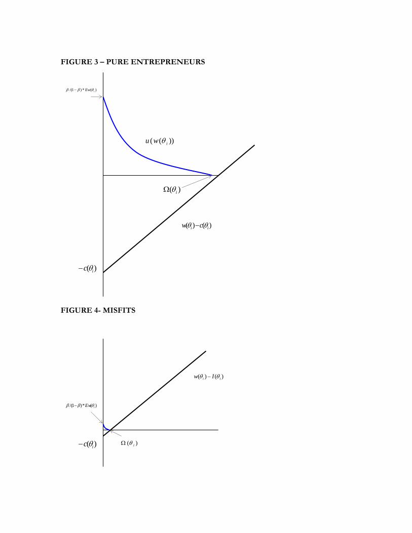
FIGURE 3 – PURE ENTREPRENEURS

FIGURE 4- MISFITS

)()( ii cw θθ −

))(( iwu θ

)(*)1/( iEw θββ −

)( ic θ−

)( iθΩ

)()( ii Iw θθ −

)(*)1/( iEwθββ −

)( ic θ− )( iθΩ

FIGURE 5 - BUSINESS CYCLES AND UNEMPLOYMENT IN ARGENTINA

1015

2025

Une

mploy

men

t (in %

)

2200

0024

0000

2600

0028

0000

3000

00

GDP

1994 1996 1998 2000 2002 2004quarter...

GDP Unemployment (in %)

Note: Variables expressed in real terms. FIGURE 6- EVOLUTION OF HOURLY WAGES

-.3-.2

-.10

.1

Inco

me grow

th

.8.9

11.1

1.2

Log Hou

rly W

age

1994 1996 1998 2000 2002Year, Wave...

Log Hourly Wage Income growth

Note: Pooled EPH data (1995-2003). Variables expressed in real terms. FIGURE 7- SELF-EMPLOYMENT AND THE BUSINESS CYCLE

.11

.115

.12

.125

Own-ac

coun

t rate

.18

.181

.182

.183

.184

.185

Self-e

mploy

men

t rate

1994 1996 1998 2000 2002(mean) period ...

Self-employment rate Own-account rate

Note: Pooled Eph data (1995-2003). Rates expressed as a proportion of the total active labor force.

FIGURE 8- WAGE PREMIUM

-.05

0.05

.1.15

.2

1994 1996 1998 2000 2002Year, Wav e

wrt All SE wrt Own-Accountwrt SE w/employ ees

Note: Pooled EPH data (1995-2003). Premiums in levels are obtained as in section 3.1. FIGURE 9- SCHOOLING AND TRANSITION TO SELF-EMPLOYMENT

.25

.3.35

.4Sal to

SE (w

ith employ

ees)

.08

.082

.084

.086

.088

Sal to

SE

9.6

9.8

1010

.210

.4Mea

n Sc

hooling (S

al to

SE)

1994 1996 1998 2000 2002Year, Wav e

Mean Schooling (Sal to SE) Sal to SESal to SE (with employ ees)

Note: Pooled EPH data (1995-2003). SE: self-employed workers, Sal: salaried workers FIGURE 10- SCHOOLING AND TRANSITION TO SALARIED POSITIONS.

.216

.218

.22

.222

.224

.226

Pro

portion

SE to

Sal

99.5

1010

.5Mea

n Sch

oolin

g (S

E to S

al)

1994 1996 1998 2000 2002Year, Wav e

Mean Schooling (SE to Sal) Proportion SE to Sal

Note: Pooled EPH data (1995-2003). SE: self-employed workers, Sal: salaried workers

FIGURE 11- SCHOOLING AND TRANSITION FROM UNEMPLOYMENT

.18

.19

.2.21

.22

.23

U to

SE (w

ith employ

ees)

.18

.19

.2.21

.22

U to

SE

8.4

8.6

8.8

99.2

9.4

Mea

n Sch

oolin

g (U

to SE)

1994 1996 1998 2000 2002Year, Wave...

Mean Schooling (U to SE) U to SEU to SE (w ith employees)

Note: Pooled EPH data (1995-2003). SE: self-employed workers, Sal: salaried workers, U: unemployed. EFFECT OF AGE AND EDUCATION ON THE LIKELIHOOD OF ENTRY FIGURE 12-A FROM SALARIED POSITIONS INTO SELF-EMPLOYMENT (PROBIT SPECIFICATION)

05

10

15

Education

20

30

4050

60

Age

-0.14-0.12-0.1-0.08-0.06

% Chg . P

05

10

15

tion

-0-0--

Note: Constructed using the coefficients of Table 5 (Column 2). Horizontal and Vertical axes correspond to Education and Age. The height of the box refers to the change in marginal probability.

FIGURE 12-B FROM UNEMPLOYMENT INTO SELF-EMPLOYMENT AND SALARIED POSITIONS (MULTINOMIAL LOGIT SPECIFICATION)

-Self-Employment -Salaried Position

0

5

10

15

Education

20

30

40

5060

Age

-0.2

-0.1

0

% Chg . P

0

5

10

15

ation

0

5

10

15

Education

20

30

40

5060

Age

-0.4-0.3-0.2-0.1

0

% Chg. P

0

5

10

15

ation

Note: Constructed using the coefficients of Table 6 (Column 3 and 4 respectively). See additional notes in Table 5. FIGURE 12-C FROM SALARIED POSITIONS INTO OWN-ACCOUNT AND ENTREPRENEUR WITH EMPLOYEES POSITIONS (MULTINOMIAL LOGIT)

-Own-Account -Entrepreneur with Employees

0

5

10

15

Education

20

30

40

5060

Age

-0.08

-0.06% Chg . P

0

5

10

15

ation

0

5

10

15

Education

20

30

40

5060

Age

00.010.020.03

% Chg. P

0

5

10

15

ation

Notes: Constructed using the coefficients of Table 8 (Column 3 and 4 respectively). See additional notes in table 5.

FIGURE 13 EFFECT OF UNEMPLOYMENT DURATION IN THE PROBABILITY OF ENTRY INTO SELF-EMPLOYMENT AND SALARIED POSITIONS

10 20 30 40 50 60 70Unempl duration

-0.1

-0.08

-0.06

-0.04

-0.02

0.02

0.04% Chg . P

Note: Constructed using the coefficients of Table 6. Self-Employment (dashed blue), Salaried (solid red).