microeconomics notes - all …€¦ · microeconomics notes ... difference between business...
TRANSCRIPT

http://www.allonlinefree.com/
http://www.allonlinefree.com/
MICROECONOMICS NOTES
UNIT-1
NATURE OF ECONOMICS
Under this, we generally discuss whether Economics is science or art or both and if it is a science whether it is a positive science or a normative science or both.
Economics - As a science and as an art:
Often a question arises - whether Economics is a science or an art or both.
(a) Economics is a science: A subject is considered science if It is a systematised body of knowledge which studies the relationship between cause and effect. It is capable of measurement. It has its own methodological apparatus. It should have the ability to forecast.
If we analyse Economics, we find that it has all the features of science. Like science it studies cause and effect relationship between economic phenomena. To understand, let us take the law of demand. It explains the cause and effect relationship between price and demand for a commodity. It says, given other things constant, as price rises, the demand for a commodity falls and vice versa. Here the cause is price and the effect is fall in quantity demanded. Similarly like science it is
www.allo
nline
free.
com

http://www.allonlinefree.com/
http://www.allonlinefree.com/
capable of being measured, the measurement is in terms of money. It has its own methodology of study (induction and deduction) and it forecasts the future market condition with the help of various statistical and non-statistical tools. But it is to be noted that Economics is not a perfect science. This is because Economists do not have uniform opinion about a particular event. The subject matter of Economics is the economic behaviour of man which is highly unpredictable. Money which is used to measure outcomes in Economics is itself a dependent variable.
It is not possible to make correct predictions about the behaviour of economic variables.
(b) Economics is an art: Art is nothing but practice of knowledge. Whereas science teaches us to know art teaches us to do. Unlike science which is theoretical, art is practical. If we analyse Economics, we find that it has the features of an art also. Its various branches, consumption, production, public finance, etc. provide practical solutions to various economic problems. It helps in solving various economic problems which we face in our day-to-day life.
Thus, Economics is both a science and an art. It is science in its methodology and art in its application. Study of unemployment problem is science but framing suitable policies for reducing the extent of unemployment is an art.
SCOPE OF MANAGERIAL OR BUSINESS ECONOMICS
Managerial economics is a developing science which generates the countless problems to determine its scope in a clear-cut way. From the following fields, we can examine the scope of business economics.
1. Demand analysis and forecasting. The foremost aspect regarding scope is demand analysis and forecasting. A business firm is an economic unit which transforms. productive resources into saleable
www.allo
nline
free.
com

http://www.allonlinefree.com/
http://www.allonlinefree.com/
goods. Since all output is meant to be sold, accurate estimates of demand help a firm in minimising its costs of production and storage. A firm must decide its total output before preparing its production schedule and deciding on the resources to be employed. Demand forecasts serves as a guide to the management for maintaining its market share in competition with its rivals, thereby securing its profit.
2. Cost and production analysis. A firm's profitability depends much on its costs of production. A wise manager would prepare cost estimates of a range of output, identify the factors causing variations in costs and choose the cost-minimising output level, taking also into consideration the degree of uncertainty in production and cost calculations. Production process are under the charge of engineers but the business manager works to carry out the production function analysis in order to avoid wastages of materials and time. Sound pricing policies depend much on cost control. The main topics discussed under cost and production analysis are: Cost concepts, cost-output relationships, Economies and Diseconomies of scale and cost control.
www.allo
nline
free.
com

http://www.allonlinefree.com/
http://www.allonlinefree.com/
3. Pricing decisions, policies and practices. Another task before a business manager is the pricing of a product. Since a firm's income and profit depend mainly on the price decision, the pricing policies and all such decisions are to be taken after careful analysis of the nature of the market in which the firm operates. The important topics covered in this field of study are : Market Structure Analysis, Pricing Practices and Price Forecasting.
4. Profit management. Each and every business firms are tended for earning profit, it is profit which provides the chief measure of success of a firm in the long period. Economists tells us that profits are the reward for uncertainity bearing and risk taking. A successful business manager is one who can form more or less correct estimates of costs and revenues at different levels of output. The more successful a manager is in reducing uncertainity, the higher are the profits earned by him. It is therefore, profit-planning and profit measurement constitute the most challenging area of business economics.
5. Capital management. Still another most challenging problem for a modern business manager is of planning capital investment. Investments are made in the plant and
machinery and buildings which are very high. Therefore, capital management require top- level decisions. It means capital management i.e., planning and control of capital expenditure. It deals with Cost of capital, Rate of Return and Selection of projects.
www.allo
nline
free.
com

http://www.allonlinefree.com/
http://www.allonlinefree.com/
6. Inventory management: A firm should always keep an ideal quantity of stock. If the stock is too much, the capital is unnecessarily locked up in inventories At the same time if the level of inventory is low, production will be interrupted due to non-availability of materials. Hence, a firm always prefers to have an optimum quantity of stock. Therefore, managerial economics will use some methods such as ABC analysis, inventory models with a view to minimising the inventory cost.
7. Linear programming and theory of games : Linear programming and theory of games have came to be regarded as part of managerial economics recently.
8. Environmental issues: There are certain issues of macroeconomics which also form a part of managerial economics. These issues relate to general business, social and political environment in which a business enterprise operates.
9. Business cycles: Business cycles affect business decisions. They refer to regular fluctuations in economic activities in the country. The different phases of business cycle are depression, recovery, prosperity, boom and recession.
Thus, managerial economics comprises both micro and macro-economic theories. The subject matter of managerial economics consists of all those economic concepts, theories and tools of analysis which can be used to analyse the business environment and to find out solution to practical business problems.
DIFFERENCE BETWEEN BUSINESS ECONOMICS AND ECONOMICS
Economics is the social science that studies the production, distribution, and consumption of goods and services. Economics aims to explain how economies work and how economic agents
www.allo
nline
free.
com

http://www.allonlinefree.com/
http://www.allonlinefree.com/
interact. Economic analysis is applied throughout society, in business and finance but also in crime, education, the family, health, law, politics, religion, social institutions, and war. Economic textbooks distinguish between microeconomics ("small" economics), which examines the economic behavior of agents (including individuals and firms) and "macroeconomics" ("big" economics), addressing issues of unemployment, inflation, monetary and fiscal policy. Business economics (also called managerial economics), is a branch of economics that applies microeconomic analysis to specific business decisions. As such, it bridges economic theory and economics in practice. It draws heavily from quantitative techniques such as regression analysis and correlation, Lagrangian calculus (linear). If there is a unifying theme that runs through most of business economics it is the attempt to optimize business decisions given the firm's objectives and given constraints imposed by scarcity, for example through the use of operations research and programming.
MICRO Vs. MACRO ECONOMICS
Micro Economics:
1. Micro Economics studies the problems of individual economic units such as a firm, an industry, a consumer etc.
2. Micro Economic studies the problems of price determination, resource allocation etc.
3. While formulating economic theories, Micro Economics assumes that other things remain constant.
www.allo
nline
free.
com

http://www.allonlinefree.com/
http://www.allonlinefree.com/
4. The main determinant of Micro Economics is price.
Macro Economics:
1. Macro Economics studies economic problems relating to an economy viz., National Income, Total Savings etc.
2. Macro Economics studies the problems of economic growth, employment and income determination etc.
3. In Micro Economics economic variables are mutually inter-related independently.
4. In Micro Economics economic variables are mutually inter-related independently.
OPPORTUNITY COST
Opportunity cost is the cost of any activity measured in terms of the value of the best alternative that is not chosen (that is foregone). It is the sacrifice related to the second best choice available to someone, or group, who has picked among several mutually exclusive choices.
[1] The opportunity cost is also
the cost of the foregone products after making a choice. Opportunity cost is a key concept in economics, and has been described as expressing "the basic relationship between scarcity and choice".
[2] The notion of opportunity cost
plays a crucial part in ensuring that scarce resources are used efficiently.
[3] Thus, opportunity costs are not restricted to monetary
or financial costs: the real cost of output foregone, lost time, pleasure or any other benefit that provides utility should also be considered opportunity costs.
Explicit costs
www.allo
nline
free.
com

http://www.allonlinefree.com/
http://www.allonlinefree.com/
Explicit costs are opportunity costs that involve direct monetary payment by producers. The opportunity cost of the factors of production not already owned by a producer is the price that the producer has to pay for them. For instance, a firm spends $100 on electrical power consumed, their opportunity cost is $100. The firm has sacrificed $100, which could have been spent on other factors of production.
Implicit costs
Implicit costs are the opportunity costs that involve only factors of production that a producer already owns. They are equivalent to what the factors could earn for the firm in alternative uses, either operated within the firm or rent out to other firms. For example, a firm pays $300 a month all year for rent on a warehouse that only holds product for six months each year. The firm could rent the warehouse out for the unused six months, at any price (assuming a year-long lease requirement), and that would be the cost that could be spent on other factors of production.
TIME VALUE OF MONEY
The time value of money is the value of money figuring in a given amount of interest earned over a given amount of time. The time value of money is the central concept in finance theory.
For example, $100 of today's money invested for one year and earning 5% interest will be worth $105 after one year. Therefore, $100 paid now or $105 paid exactly one year from now both
www.allo
nline
free.
com

http://www.allonlinefree.com/
http://www.allonlinefree.com/
have the same value to the recipient who assumes 5% interest; using time value of money terminology, $100 invested for one year at 5% interest has a future value of $105.
[1]This notion dates at least to Martín de
Azpilcueta (1491–1586) of the School of Salamanca.
The method also allows the valuation of a likely stream of income in the future, in such a way that the annual incomes are discounted and then added together, thus providing a lump-sum "present value" of the entire income stream.
All of the standard calculations for time value of money derive from the most basic algebraic expression for the present value of a future sum, "discounted" to the present by an amount equal to the time value of money. For example, a sum of FV to be received in one year is discounted (at the rate of interest r) to give a sum of PV at present: PV = FV − r·PV = FV/(1+r).
MARGINALISM
Marginalism refers to the use of marginal concepts in economic theory. Marginalism is associated with arguments concerning changes in the quantity used of a good or service, as opposed to some notion of the over-all significance of that class of good or service, or of some total quantity thereof.
Market Forces and Equilibrium
www.allo
nline
free.
com

http://www.allonlinefree.com/
http://www.allonlinefree.com/
Summary: Explains market equilibrium and the relation between market demand and supply. Details how market forces determinepricing.
Market equilibrium is the situation where, at a certain price level, the quantity demanded by consumers and the quantity supplied by producers of a particular commodity are equal. This means that the market is completely clear of excess supply and demand, and there isn't any tendency for change to either price or quantity. At market equilibrium, consumers are willing to pay the market pricefor the commodity in question and producers are willing and able to sell their goods at that market priceand at that quantity. The price mechanism is a device used to determine the equilibriumprice and equilibrium quantity of goods and also demonstrates how market forces work to achieve market equilibrium. The price mechanism assumes that there is no intervention on the part of the government and the market structure is a pure.
www.allo
nline
free.
com

http://www.allonlinefree.com/
http://www.allonlinefree.com/
UNIT-2
Cardinal Utility Analysis/Approach:
Definition and Explanation:
Human wants are unlimited and they are of different intensity. The means at the disposal of a man are not only scarce but they have alternative uses. As a result of scarcity of recourses, the consumer cannot satisfy all his wants. He has to choose as to which want is to be satisfied first and which afterward if the recourses permit. The consumer is confronted in making a choice.
For example, a man is thirsty. He goes to the market and satisfy his thirst by purchasing coca cola instead of tea. We are here to examine the economic forces which make him purchase a particular commodity. The answer is simple. The consumer buys a commodity because it gives
www.allo
nline
free.
com

http://www.allonlinefree.com/
http://www.allonlinefree.com/
him satisfaction. In technical term, a consumer purchases a commodity because it has utility for him. We now examine the tools which are used in the analyzes of consumer behavior.
Assumptions of Cardinal Utility Analysis:
The main assumption or premises on which the cardinal utility analysis rests are as under.
(i) Rationality. The consumer is rational. He seeks to maximize satisfaction from the limited income which is at his disposal.
(ii) Utility is cardinally measurable. The utility can be measured in cardinal numbers such as 1, 3, 10, 15, etc. The utility is expressed in imaginary cardinal numbers tells us a great deal about the preference of the consumer for a good.
(iii) Marginal utility of money remains constant. Another important premise of cardinal utility of money spent on the purchase of a good or service should remain constant.
(iv) Diminishing marginal utility. It is also assumed that the marginal utility obtained from the consumption of a good diminishes continuously as its consumption is increased.
(v) Independent utilities. According to the Cardinalist school, the utility which is derived from the consumption of a good is a function of the quantity of that good alone. If does not depend at all upon the quantity consumed of other goods. The goods, we can say, possess
www.allo
nline
free.
com

http://www.allonlinefree.com/
http://www.allonlinefree.com/
independent utilities and are additive. Law of Diminishing Marginal Utility:
Definition and Statement of the Law:
The law of diminishing marginal utility describes a familiar and fundamental tendency of human behavior. The law of diminishing marginal utility states that:
“As a consumer consumes more and more units of a specific commodity, the utility from the successive units goes on diminishing”.
“The additional benefit which a person derives from an increase of his stock of a thing diminishes with every increase in the stock that already has”.
Law is Based Upon Three Facts:
The law of diminishing marginal utility is based upon three facts. First, total wants of a man are unlimited but each single want can be satisfied. As a man gets more and more units of a commodity, the desire of his for that good goes on falling. A point is reached when the consumer no longer wants any more units of that good.Secondly, different goods are not perfect substitutes for each other in the satisfaction of various particular wants. As such the marginal utility will decline as the consumer gets additional units of a specific good.Thirdly, the marginal utility of money is constant given the consumer’s wealth.
Explanation and Example of Law of Diminishing Marginal Utility:
www.allo
nline
free.
com

http://www.allonlinefree.com/
http://www.allonlinefree.com/
This law can be explained by taking a very simple example. Suppose, a man is very thirsty. He goes to the market and buys one glass of sweet water. The glass of water gives him immense pleasure or we say the first glass of water has great utility for him. If he takes second glass of water after that, the utility will be less than that of the first one. It is because the edge of his thirst has been blunted to a great extent. If he drinks third glass of water, the utility of the third glass will be less than that of second and so on.
The utility goes on diminishing with the consumption of every successive glass water till it drops down to zero. This is the point of satiety. It is the position of consumer’s equilibrium or maximum satisfaction. If the consumer is forced further to take a glass of water, it leads to disutility causing total utility to decline. The marginal utility will become negative.
Schedule of Law of Diminishing Marginal Utility:
Units Total Utility Marginal Utility
1st glass 20 20
2nd glass 32 12
3rd glass 40 8
4th glass 42 2
5th glass 42 0
6th glass 39 -3
From the above table, it is clear that in a given span of time, the first glass of water to a thirsty man gives 20 units of utility. When he takes second glass of water, the
www.allo
nline
free.
com

http://www.allonlinefree.com/
http://www.allonlinefree.com/
marginal utility goes on down to 12 units; When he consumes fifth glass of water, the marginal utility drops down to zero and if the consumption of water is forced further from this point, the utility changes into disutility (-3).
Curve/Diagram of Law of Diminishing Marginal Utility:
The law of diminishing marginal utility can also be represented by a diagram.
Assumptions of Law of Diminishing Marginal Utility:
The law of diminishing marginal utility is true under certain assumptions. These assumptions are as under:
(i) Rationality: In the cardinal utility analysis, it is assumed that the consumer is rational. He aims at maximization of utility subject to availability of his income.
(ii) Constant marginal utility of money: It is assumed in the theory that the marginal utility of money based for
www.allo
nline
free.
com

http://www.allonlinefree.com/
http://www.allonlinefree.com/
purchasing goods remains constant. If the marginal utility of money changes with the increase or decrease in income, it then cannot yield correct measurement of the marginal utility of the good.
(iii) Diminishing marginal utility: Another important assumption of utility analysis is that the utility gained from the successive units of a commodity diminishes in a given time period.
(iv) Utility is additive: In the early versions of the theory of consumer behavior, it was assumed that the utilities of different commodities are independent. The total utility of each commodity is additive.
U = U1 (X
1) + U
2 (X
2) + U
3 (X
3)………. U
n (X
n)
(v) Consumption to be continuous: It is assumed in this law that the consumption of a commodity should be continuous. If there is interval between the consumption of the same units of the commodity, the law may not hold good. For instance, if you take one glass of water in the morning and the 2nd at noon, the marginal utility of the 2nd glass of water may increase.
(vi) Suitable quantity: It is also assumed that the commodity consumed is taken in suitable and reasonable units. If the units are too small, then the marginal utility instead of falling may increase up to a few units.
(vii) Character of the consumer does not change: The law holds true if there is no change in the character of the consumer. For example, if a consumer develops a taste
www.allo
nline
free.
com

http://www.allonlinefree.com/
http://www.allonlinefree.com/
for wine, the additional units of wine may increase the marginal utility to a drunkard.
(viii) No change to fashion: Customs and tastes: If there is a sudden change in fashion or customs or taste of a consumer, it can than make the law inoperative.
(ix) No change in the price of the commodity: there should be any change in the price of that commodity as more units are consumed.
Law of Equi-Marginal Utility:
Definition and Statement of Law of Equi-Marginal Utility:
The law of equi-marginal utility is simply an extension of law of diminishing marginal utility to two or more than two commodities. The law of equilibrium utility is known, by various names. It is named as the Law of Substitution, the Law of Maximum Satisfaction, the Law of Indifference, the Proportionate Rule and the Gossen’s Second Law.
In cardinal utility analysis, this law is stated by Lipsey in the following words:
“The household maximizing the utility will so allocate the expenditure between commodities that the utility of the last penny spent on each item is equal”
As we know, every consumer has unlimited wants. However, the income this disposal at any time is limited. The consumer is, therefore, faced with a choice among many commodities that he can and would like to pay. He,
www.allo
nline
free.
com

http://www.allonlinefree.com/
http://www.allonlinefree.com/
therefore, consciously or unconsciously compress the satisfaction which he obtains from the purchase of the commodity and the price which he pays for it. If he thinks the utility of the commodity is greater or at-least equal to the loss of utility of money price, he buys that commodity.
Assumptions of Law of Equi-Marginal Utility:
The main assumptions of the law of equi-marginal utility are as under.
(i) Independent utilities. The marginal utilities of different commodities are independent of each other and diminish with more and more purchases.
(ii) Constant marginal utility of money. The marginal utility of money remains constant to the consumer as he spends more and more of it on the purchase of goods.
(iii) Utility is cardinally measurable.
(iv) Every consumer is rational in the purchase of goods.
Example and Explanation of Law of Equi-Marginal Utility:
The doctrine of equi-marginal utility can be explained by taking an example. Suppose a person has $5 with him whom he wishes to spend on two commodities, tea and cigarettes. The marginal utility derived from both these commodities is as under:
Schedule:
Units of MU of Tea MU of
www.allo
nline
free.
com

http://www.allonlinefree.com/
http://www.allonlinefree.com/
Money Cigarettes
1 10 12
2 8 10
3 6 8
4 4 6
5 2 3
$5 Total Utility = 30 Total Utility = 30
A rational consumer would like to get maximum satisfaction from $5.00. He can spend money in three ways:
(i) $5 may be spent on tea only.
(ii) $5 may be utilized for the purchase of cigarettes only.
(iii) Some rupees may be spent on the purchase of tea and some on the purchase of cigarettes.
Curve/Diagram of Law of Equi-Marginal Utility:
The law of equi-marginal utility can be explained with the help of diagrams.
www.allo
nline
free.
com

http://www.allonlinefree.com/
http://www.allonlinefree.com/
Theory of Ordinal Utility/Indifference Curve Analysis:
Definition and Explanation:
The indifference curve indicates the various combinations of two goods which yield equal satisfaction to the consumer. By definition:
"An indifference curve shows all the various combinations of two goods that give an equal amount of satisfaction to a consumer".
These economist are the of view that it is wrong to base the theory of consumption on two assumptions:
(i) That there is only one commodity which a person will buy at one time.
(ii) The utility can be measured.
Their point of view is that utility is purely subjective and is immeasurable. Moreover an individual is interested in a combination of related goods and in the purchase of one commodity at one time. So they base the theory of
www.allo
nline
free.
com

http://www.allonlinefree.com/
http://www.allonlinefree.com/
consumption on the scale of preference and the ordinal ranks or orders his preferences.
Assumptions:
The ordinal utility theory or the indifference curve analysis is based on four main assumptions.
(i) Rational behavior of the consumer: It is assumed that individuals are rational in making decisions from their expenditures on consumer goods.
(ii) Utility is ordinal: Utility cannot be measured cardinally. It can be, however, expressed ordinally. In other words, the consumer can rank the basket of goods according to the satisfaction or utility of each basket.
(iii) Diminishing marginal rate of substitution: In the indifference curve analysis, the principle of diminishing marginal rate of substitution is assumed.
(iv) Consistency in choice: The consumer, it is assumed, is consistent in his behavior during a period of time. For insistence, if the consumer prefers combinations of A of good to the combinations B of goods, he then remains consistent in his choice. His preference, during another period of time does not change. Symbolically, it can be expressed as:
If A > B, then B > A
(iv) Consumer’s preference not self contradictory: The consumer’s preferences are not self contradictory. It
www.allo
nline
free.
com

http://www.allonlinefree.com/
http://www.allonlinefree.com/
means that if combinations A is preferred over combination B is preferred over C, then combination A is preferred over combination A is preferred over C. Symbolically it can be expressed:
If A > B and B > C, then A > C
(v) Goods consumed are substitutable: The goods consumed by the consumer are substitutable. The utility can be maintained at the same level by consuming more of some goods and less of the other. There are many combinations of the two commodities which are equally preferred by a consumer and he is indifferent as to which of the two he receives.
Example:
For example, a person has a limited amount of income which he wishes to spend on two commodities, rice and wheat. Let us suppose that the following commodities are equally valued by him:
Various Combinations:
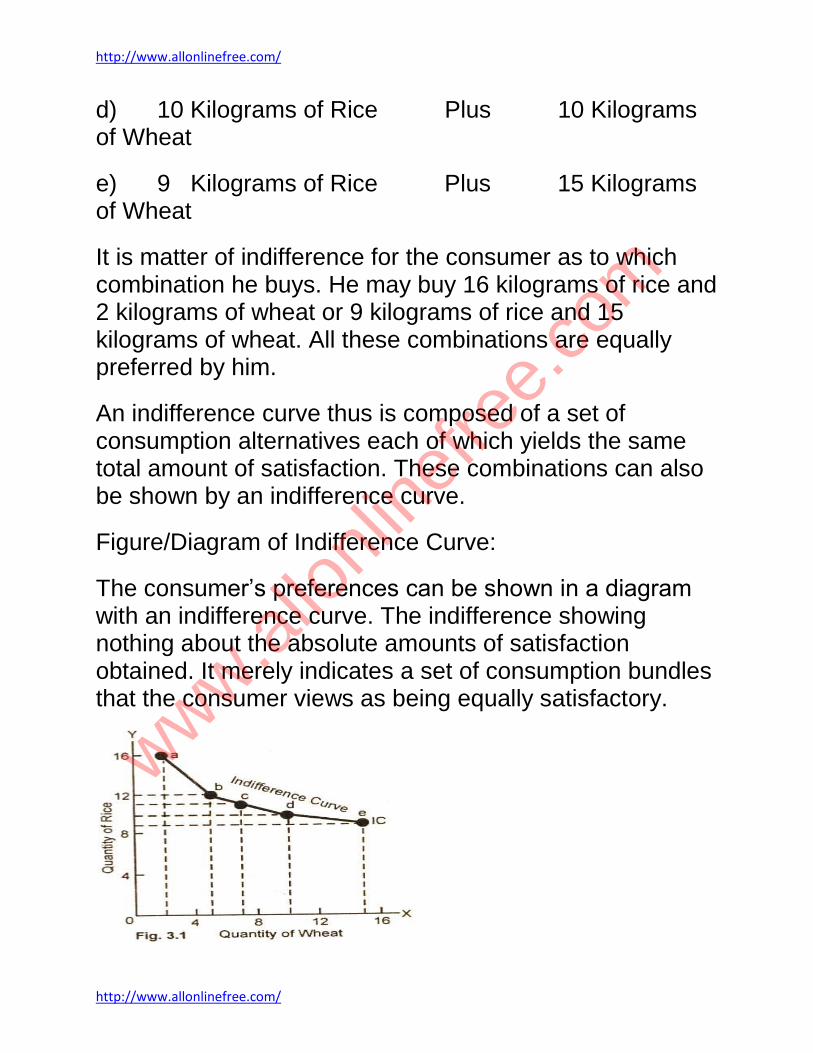
a) 16 Kilograms of Rice Plus 2 Kilograms of Wheat
b) 12 Kilograms of Rice Plus 5 Kilograms of Wheat
c) 11 Kilograms of Rice Plus 7 Kilograms of Wheat
www.allo
nline
free.
com
http://www.allonlinefree.com/
http://www.allonlinefree.com/
d) 10 Kilograms of Rice Plus 10 Kilograms of Wheat
e) 9 Kilograms of Rice Plus 15 Kilograms of Wheat
It is matter of indifference for the consumer as to which combination he buys. He may buy 16 kilograms of rice and 2 kilograms of wheat or 9 kilograms of rice and 15 kilograms of wheat. All these combinations are equally preferred by him.
An indifference curve thus is composed of a set of consumption alternatives each of which yields the same total amount of satisfaction. These combinations can also be shown by an indifference curve.
Figure/Diagram of Indifference Curve:
The consumer’s preferences can be shown in a diagram with an indifference curve. The indifference showing nothing about the absolute amounts of satisfaction obtained. It merely indicates a set of consumption bundles that the consumer views as being equally satisfactory.
www.allo
nline
free.
com

http://www.allonlinefree.com/
http://www.allonlinefree.com/
In fig. 3.1 we measure the quantity of wheat along X-axis (in kilograms) and along Y-axis, the quantity of rice (in kilograms). IC is an indifference curve.
It is shown in the diagram that a consumer may buy 12 kilograms of rice and 5 kilograms of wheat or 9 kilograms of rice and 15 kilogram of wheat. Both these combinations are equally preferred by him and he is indifferent to these two combinations. When the scale of preference of the consumer is graphed, by joining the points a, b, c, d, e, we obtain an Indifference Curve IC.
Every point on indifference curve represents a different combination of the two goods and the consumer is indifferent between any two points on the indifference curve. All the combinations are equally desirable to the consumer. The consumer is indifferent as to which combination he receives. The Indifference Curve IC thus is a locus of different combinations of two goods which yield the same level of satisfaction.
Marginal Rate of Substitution (MRS):
The necessity is to study the behavior of the consumer as to how he prefers one commodity to another and maintains the same level of satisfaction.
For example, there are two goods X and Y which are not perfect substitute of each other. The consumer is prepared to exchange goods X for Y. How many units of Y should be given for one unit of X to the consumer so that his level of satisfaction remains the same?
www.allo
nline
free.
com

http://www.allonlinefree.com/
http://www.allonlinefree.com/
The rate or ratio at which goods X and Y are to be exchanged is known as the marginal rate of substitution (MRS). In the words of Hicks:
“The marginal rate of substitution of X for Y measures the number of units of Y that must be scarified for unit of X gained so as to maintain a constant level of satisfaction”.
Marginal rate of substitution (MRS) can also be defined as:
“The ratio of exchange between small units of two commodities, which are equally valued or preferred by a consumer”.
Formula:
MRSxy = ∆Y
∆X
It may here be noted that the marginal rate of substitution (MRS) is the personal exchange rate of the consumer in contrast to the market exchange rate.
Diminishing Marginal Rate of Substitution:
In other words, as the consumer has more and more units of good X, he is prepared to forego less and less of good Y.
This behavior showing falling MRS of good X for good Y and yet to remain at the same level of satisfaction is known as diminishing marginal rate of substitution.
www.allo
nline
free.
com

http://www.allonlinefree.com/
http://www.allonlinefree.com/
Diagram/Figure:
The concept of marginal rate of substitution (MRS) can also be illustrated with the help of the diagram.
In the fig. 3.3 above as the consumer moves down from combination 1 to combination 2, the consumer is willing to give up 4 units of good Y (∆Y) to get an additional unit of good X (∆X).
When the consumer slides down from combinations 2, 3 and 4, the length of ∆Y becomes smaller and smaller, while the length of ∆X is remain the same. This shows that as the stock of the consumer for good X increases, his stock of good Y decreases.
He, therefore, is willing to give less units of Y to obtain an additional unit of good X. In other words, the MRS of good X for good Y falls as the consumer has more of good X and less of good Y. The indifference curve IC slopes downward from left to the right. This means a negative and diminishing rate of substitution of one commodity for the other.
www.allo
nline
free.
com

http://www.allonlinefree.com/
http://www.allonlinefree.com/
Importance of Marginal Rate of Substitution (MRS):
(i) Measures utility ordinally: The concept of MRS is superior to that of utility concept because it is more realistic and scientific than the theory of utility. It does not measure the utility of a commodity in isolation without reference to other commodities but takes into consideration the combination of related goods to which a consumer is interested to purchase.
(ii) A relative concept: The concept of marginal rate of substitution has the advantage that it is relative and not absolute like the utility concept given by Marshall. It is free from any assumptions concerning the possibility of a quantitative measurement of utility.
Budget Line:
Definition and Explanation:
The understanding of the concept of budget line is essential for knowing the theory of consumer’s equilibrium.
"A budget line or price line represents the various combinations of two goods which can be purchased with a given money income and assumed prices of goods".
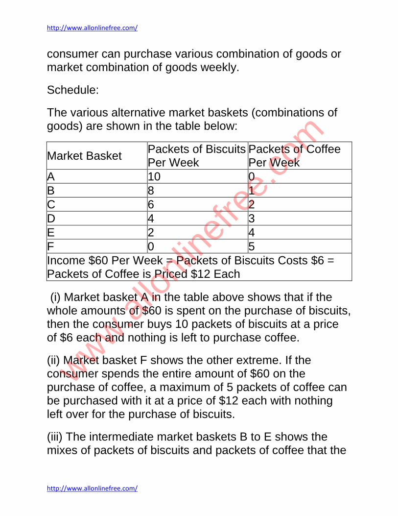
For example, a consumer has weekly income of $60. He purchases only two goods, packets of biscuits and packets of coffee. The price of each packet of biscuits is $6 and the price of each packet of coffee is $12. Given the assumed income and the price, of the two goods, the
www.allo
nline
free.
com
http://www.allonlinefree.com/
http://www.allonlinefree.com/
consumer can purchase various combination of goods or market combination of goods weekly.
Schedule:
The various alternative market baskets (combinations of goods) are shown in the table below:
Market Basket Packets of Biscuits Per Week
Packets of Coffee Per Week
A 10 0
B 8 1
C 6 2
D 4 3
E 2 4
F 0 5
Income $60 Per Week = Packets of Biscuits Costs $6 = Packets of Coffee is Priced $12 Each
(i) Market basket A in the table above shows that if the whole amounts of $60 is spent on the purchase of biscuits, then the consumer buys 10 packets of biscuits at a price of $6 each and nothing is left to purchase coffee.
(ii) Market basket F shows the other extreme. If the consumer spends the entire amount of $60 on the purchase of coffee, a maximum of 5 packets of coffee can be purchased with it at a price of $12 each with nothing left over for the purchase of biscuits.
(iii) The intermediate market baskets B to E shows the mixes of packets of biscuits and packets of coffee that the
www.allo
nline
free.
com

http://www.allonlinefree.com/
http://www.allonlinefree.com/
cost a total of $60. For example, in combination of market basket C, the consumer can purchase 6 packets of biscuits and 2 packets of coffee with a total cost of $60.
Budget Line:
The budget line is an important element analysis of consumer behavior. The indifference map shows people’s preferences for the combination of two goods. The actual choices they will make, however, depends on their income. The budget line is drawn as a continuous line. It identifies the options from which the consumer can choose the combination of goods.
Diagram/Figure:
In the fig. 3.9 the line AF shows the various combinations of goods the consumer can purchase. This line is called the budget line.
The slope of the budget line indicates how many packets of biscuits a purchaser must give up to buy one more packet of coffee. For example, the slope at point B on the budget line is ∆Y / ∆X or two packets of biscuits 1 = packet
www.allo
nline
free.
com

http://www.allonlinefree.com/
http://www.allonlinefree.com/
of coffee. This indicates that a move from B to C involves sacrificing two packets of biscuits to gain an additional one packet of coffee. Since AF budget line is straight, the slope is constant at -2 packets of biscuits per one packet of coffee at all points along the line.
Consumer's Equilibrium Through Indifference Curve Analysis:
Definition:
"The term consumer’s equilibrium refers to the amount of goods and services which the consumer may buy in the market given his income and given prices of goods in the market".
The aim of the consumer is to get maximum satisfaction from his money income. Given the price line or budget line and the indifference map:
"A consumer is said to be in equilibrium at a point where the price line is touching the highest attainable indifference curve from below".
Conditions:
Thus the consumer’s equilibrium under the indifference curve theory must meet the following two conditions:
First: A given price line should be tangent to an indifference curve or marginal rate of satisfaction of good X for good Y (MRSxy) must be equal to the price ratio of the two goods. i.e.
www.allo
nline
free.
com

http://www.allonlinefree.com/
http://www.allonlinefree.com/
MRSxy = Px / Py
Second: The second order condition is that indifference curve must be convex to the origin at the point of tangency.
Assumptions:
The following assumptions are made to determine the consumer’s equilibrium position.
(i) Rationality: The consumer is rational. He wants to obtain maximum satisfaction given his income and prices.
(ii) Utility is ordinal: It is assumed that the consumer can rank his preference according to the satisfaction of each combination of goods.
(iii) Consistency of choice: It is also assumed that the consumer is consistent in the choice of goods.
(iv) Perfect competition: There is perfect competition in the market from where the consumer is purchasing the goods.
(v) Total utility: The total utility of the consumer depends on the quantities of the good consumed.
Explanation:
The consumer’s consumption decision is explained by combining the budget line and the indifference map. The consumer’s equilibrium position is only at a point where the price line is tangent to the highest attainable indifference curve from below.
www.allo
nline
free.
com

http://www.allonlinefree.com/
http://www.allonlinefree.com/
(1) Budget Line Should be Tangent to the Indifference Curve:
The consumer’s equilibrium in explained by combining the budget line and the indifference map.
Diagram/Figure:
In the diagram 3.11, there are three indifference curves IC
1, IC
2 and IC
3. The price line PT is tangent to the
indifference curve IC2 at point C. The consumer gets the
maximum satisfaction or is in equilibrium at point C by purchasing OE units of good Y and OH units of good X with the given money income.
The consumer cannot be in equilibrium at any other point on indifference curves. For instance, point R and S lie on lower indifference curve IC
1 but yield less satisfaction. As
regards point U on indifference curve IC3, the consumer
no doubt gets higher satisfaction but that is outside the budget line and hence not achievable to the consumer. The consumer’s equilibrium position is only at point C where the price line is tangent to the highest attainable indifference curve IC
2 from below.
www.allo
nline
free.
com

http://www.allonlinefree.com/
http://www.allonlinefree.com/
(2) Slope of the Price Line to be Equal to the Slope of Indifference Curve:
The second condition for the consumer to be in equilibrium and get the maximum possible satisfaction is only at a point where the price line is a tangent to the highest possible indifference curve from below. In fig. 3.11, the price line PT is touching the highest possible indifferent curve IC
2 at point C. The point C shows the combination of
the two commodities which the consumer is maximized when he buys OH units of good X and OE units of good Y.
Geometrically, at tangency point C, the consumer’s substitution ratio is equal to price ratio Px / Py. It implies that at point C, what the consumer is willing to pay i.e., his personal exchange rate between X and Y (MRSxy)is equal to what he actually pays i.e., the market exchange rate. So the equilibrium condition being Px / Pybeing satisfied at the point C is:
Price of X / Price of Y = MRS of X for Y
The equilibrium conditions given above states that the rate at which the individual is willing to substitute commodity X for commodity Y must equal the ratio at which he can substitute X for Y in the market at a given price.
(3) Indifference Curve Should be Convex to the Origin:
The third condition for the stable consumer equilibrium is that the indifference curve must be convex to the origin at
www.allo
nline
free.
com

http://www.allonlinefree.com/
http://www.allonlinefree.com/
the point of equilibrium. In other words, we can say that the MRS of X for Y must be diminishing at the point of equilibrium. It may be noticed that in fig. 3.11, the indifference curve IC
2 is convex to the origin at point C. So
at point C, all three conditions for the stable-consumer’s equilibrium are satisfied.
Summing up, the consumer is in equilibrium at point C where the budget line PT is tangent to the indifference IC
2.
The market basket OH of good X and OE of good Y yields the greatest satisfaction because it is on the highest attainable indifference curve. At point C:
MRSxy = Px / Py
THEORY OF DEMAND
Meanings and Definition of Demand:
The word 'demand' is so common and familiar with every one of us that it seems superfluous to define it. The need for precise definition arises simply because it is sometimes confused with other words such as desire, wish, want, etc.
Demand in economics means a desire to possess a good supported by willingness and ability to pay for it. If your have a desire to buy a certain commodity, say a car, but you do not have the adequate means to pay for it, it will simply be a wish, a desire or a want and not demand. Demand is an effective desire, i.e., a desire which is backed by willingness and ability to pay for a commodity in order to obtain it.
www.allo
nline
free.
com

http://www.allonlinefree.com/
http://www.allonlinefree.com/
Characteristics of Demand:
There are thus three main characteristic's of demand in economics.
(i) Willingness and ability to pay. Demand is the amount of a commodity for which a consumer has the willingness and also the ability to buy.
(ii) Demand is always at a price. If we talk of demand without reference to price, it will be meaningless. The consumer must know both the price and the commodity. He will then be able to tell the quantity demanded by him.
(iii) Demand is always per unit of time. The time may be a day, a week, a month, or a year.
Example:
For instance, when the milk is selling at the rate of $15.0 per liter, the demand of a buyer for milk is 10 liters a day. If we do not mention the period of time, nobody can guess as to how much milk we consume? It is just possible we may be consuming ten liters of milk a week, a month or a year.
Law of Demand:
Definition and Explanation of the Law:
We have stated earlier that demand for a commodity is related to price per unit of time. It is the experience of every consumer that when the prices of the commodities fall, they are tempted to purchase more. Commodities and
www.allo
nline
free.
com

http://www.allonlinefree.com/
http://www.allonlinefree.com/
when the prices rise, the quantity demanded decreases. There is, thus, inverse relationship between the price of the product and the quantity demanded. The economists have named this inverse relationship between demand and price as the law of demand.
Statement of the Law:
"Other things remaining the same, the quantity demanded of a commodity will be smaller at higher market prices and larger at lower market prices".
"Other things remaining the same, the quantity demanded increases with every fall in the price and decreases with every rise in the price".
In simple we can say that when the price of a commodity rises, people buy less of that commodity and when the price falls, people buy more of it ceteris paribus (other things remaining the same). Or we can say that the quantity varies inversely with its price. There is no doubt that demand responds to price in the reverse direction but it has got no uniform relation between them. If the price of a commodity falls by 1%, it is not necessary that may also increase by 1%. The demand can increase by 1%, 2%, 10%, 15%, as the situation demands.
Assumptions of Law of Demand:
There are three main assumptions of the Law:
(i) There should not be any change in the tastes of the consumers for goods (T).
www.allo
nline
free.
com

http://www.allonlinefree.com/
http://www.allonlinefree.com/
(ii) The purchasing power of the typical consumer must remain constant (M).
(iii) The price of all other commodities should not vary (Po).
Example of Law of Demand:
If there is a change, in the above and other assumptions, the law may not hold true. For example, according to the law of demand, other things being equal quantity demanded increases with a fall in price and diminishes with rise to price. Now let us suppose that price of tea comes down from $40 per pound to $20 per pound. The demand for tea may not increase, because there has taken place a change in the taste of consumers or the price of coffee has fallen down as compared to tea or the purchasing power of the consumers has decreased, etc., etc. From this we find that demand responds to price inversely only, if other thing remains constant. Otherwise, the chances are that, the quantity demanded may not increase with a fall in price or vice-versa.
Demand, thus, is a negative relationship between price and quantity.
Limitations/Exceptions of Law of Demand:
Though as a rule when the prices of normal goods rise, the demand them decreases but there may be a few cases where the law may not operate.
(i) Prestige goods: There are certain commodities like diamond, sports cars etc., which are purchased as a mark
www.allo
nline
free.
com

http://www.allonlinefree.com/
http://www.allonlinefree.com/
of distinction in society. If the price of these goods rise, the demand for them may increase instead of falling.
(ii) Price expectations: If people expect a further rise in the price particular commodity, they may buy more in spite of rise in price. The violation of the law in this case is only temporary.
(3) Ignorance of the consumer: If the consumer is ignorant about the rise in price of goods, he may buy more at a higher price.
(iv) Giffen goods: If the prices of basic goods, (potatoes, sugar, etc) on which the poor spend a large part of their incomes declines, the poor increase the demand for superior goods, hence when the price of Giffen good falls, its demand also falls. There is a positive price effect in case of Giffen goods.
Importance of Law of Demand:
(i) Determination of price. The study of law of demand is helpful for a trader to fix the price of a commodity. He knows how much demand will fall by increase in price to a particular level and how much it will rise by decrease in price of the commodity. The schedule of market demand can provide the information about total market demand at different prices. It helps the management in deciding whether how much increase or decrease in the price of commodity is desirable. (ii) Importance to Finance Minister. The study of this law is of great advantage to the finance minister. If by raising the
www.allo
nline
free.
com

http://www.allonlinefree.com/
http://www.allonlinefree.com/
tax the price increases to such an extend than the demand is reduced considerably. And then it is of no use to raise the tax, because revenue will almost remain the same. The tax will be levied at a higher rate only on those goods whose demand is not likely to fall substantially with the increase in price.
(iii) Importance to the Farmers. Goods or bad crop affects the economic condition of the farmers. If a goods crop fails to increase the demand, the price of the crop will fall heavily. The farmer will have no advantage of the good crop and vice-versa.
MOVEMENT ALONG Vs. SHIFT IN DEMAND CURVE
Changes in demand for a commodity can be shown through the demand curve in two ways:
(1) Movement Along the Demand Curve and
(2) Shifts of the Demand Curve.
(1) Movement Along the Demand Curve:
Demand is a multivariable function. If income and other determinants of demand such as tastes of the consumers, changes in prices of related goods, income distribution, etc., remain constant and there is a change only in price of the commodity, then we move along the same demand curve.
In this case, the demand curve remains unchanged. When, as a result of change in price, the quantity
www.allo
nline
free.
com

http://www.allonlinefree.com/
http://www.allonlinefree.com/
demanded increases or decreases, it is technically called extension and contraction in demand.
The demand curve, which represents various price quantity has a negative slope. Whenever there is a change in the quantity demanded of a good due to change, in its price, there is a movement from one point price quantity combination to another on the
same demand curve. Such a movement from one point price quantity combination to another along the same demand curve is shown in figure (4.3).
Diagram/Figure:
Here the price of a commodity falls from $8 to $2. As a result, therefore, the quantity demanded increases from 100 units to 400 units per unit of time. There is extension in demand by 300 units. This movement is from one point price quantity combination (a) to another point (b) along a given demand curve. On the other hand, if the price of a good rises from $2 to $8, there is contraction in demand by 300 units.
www.allo
nline
free.
com

http://www.allonlinefree.com/
http://www.allonlinefree.com/
We, thus, see that as a result of change in the price of a good, the consumer moves along the given demand curve. The demand curve remains the same and does not change its position. The movement along the demand curve is designated as change in quantity demanded.
(2) Shifts in Demand Curve:
Demand, as we know, is determined by many factors. When there is a change in demand due to one or more than one factors other than price, results in the shift of demand curve.
For example, if the level of income in community rises, other factors remaining the same, the demand for the goods increases. Consumers demand more goods at each price per period of me (rise or Increase in demand). The demand curve shifts upward from he original demand curve indicating that consumers at each price purchase more units of commodity per unit of time.
If there is a fall in the disposable income of the consumers or rise in the prices of close substitute of a good or decline in consumer taste or non-availability of good on credit, etc, etc., there is a reduction in demand (fall or decrease in demand). The fall or decrease in demand shifts the demand curve from the original demand curve to the left. The lower demand curve shows that consumers are able and willing to buy less of the good at each price than before.
Diagram/Figure:
www.allo
nline
free.
com

http://www.allonlinefree.com/
http://www.allonlinefree.com/
In this figure, (4.4) the original demand curve is DD/.
At a price of $12 per unit, consumers purchase 100 units. When price falls to$4 per unit, the quantity demanded increases to 500 units per unit of time. Let us assume now that level of income increases in a community. Now consumers demand 300 units of the commodity at price of $12 per unit and 600 at price of $4 per unit.
As a result, there is an upward shift of the demand curve DD
2. In case the community income falls, there is then
decrease in demand at price of $12 per unit. The quantity demanded of a good falls to 50 units. It is 300 units at price of $4 unit per period of time. There is a downward shift of the demand to the left of the original demand curve.
ELASTICITY OF DEMAND
TYPES OF Elasticity of Demand:
The quantity of a commodity demanded per unit of time depends upon various factors such as the price of a
www.allo
nline
free.
com

http://www.allonlinefree.com/
http://www.allonlinefree.com/
commodity, the money income of the prices of related goods, the tastes of the people, etc., etc.
Whenever there is a change in any of the variables stated above, it brings about a change in the quantity of the commodity purchased over a specified period of time. The elasticity of demand measures the responsiveness of quantity demanded to a change in any one of the above factors by keeping other factors constant. When the relative responsiveness or sensitiveness of the quantity demanded is measured to changes, in its price, the elasticity is said be price elasticity of demand.
(1) Price Elasticity of Demand:
Definition and Explanation:
The concept of price elasticity of demand is commonly used in economic literature. Price elasticity of demand is the degree of responsiveness of quantity demanded of a good to a change in its price. Precisely, it is defined as:
"The ratio of proportionate change in the quantity demanded of a good caused by a given proportionate change in price".
Formula:
The formula for measuring price elasticity of demand is:
Price Elasticity of Demand = Percentage in Quantity Demand
www.allo
nline
free.
com

http://www.allonlinefree.com/
http://www.allonlinefree.com/
Percentage Change in Price
Ed = Δq X P
Δp Q
The elasticity coefficient is greater than one. Therefore the demand for the good is elastic.
Types:
The concept of price elasticity of demand can be used to divide the goods in to three groups.
(i) Elastic. When the percent change in quantity of a good is greater than the percent change in its price, the demand is said to be elastic. When elasticity of demand is greater than one, a fall in price increases the total revenue (expenditure) and a rise in price lowers the total revenue (expenditure).
When with a percentage fall in price, the quantity demanded increases so
much that it results in the increase in total expenditure, the demand is
said to be elastic (Ed > 1).
For Example:
Price Per Unit ($) Quantity Demanded
Total Expenditure ($)
20 10 Pens 200.0
www.allo
nline
free.
com

http://www.allonlinefree.com/
http://www.allonlinefree.com/
10 30 Pens 300.0
(ii) Unitary Elasticity. When the percentage change in the quantity of a good demanded equals percentage in its price, the price elasticity of demand is said to have unitary elasticity. When elasticity of demand is equal to one or unitary, a rise or fall in price leaves total revenue unchanged.
When a percentage fall in price raises the quantity demanded so much as to
leave the total expenditure unchanged, the elasticity of demand is said to be
unitary (Ed = 1).
For Example:
Price Per Pen ($) Quantity Demanded
Total Expenditure ($)
10 30 300
5 60 300
(iii) Inelastic. When the percent change in quantity of a good demanded is less than the percentage change in its price, the demand is called inelastic. When elasticity of demand is inelastic or less than one, a fall in price decreases total revenue and a rise in its price increases total revenue.
When a percentage fall in price raises the quantity demanded of a good so as to cause the total expenditure
www.allo
nline
free.
com

http://www.allonlinefree.com/
http://www.allonlinefree.com/
to decrease, the demand is said to be inelastic or less than one, i.e., Ed < 1.
For Example:
Price Per Pen ($) Quantity Demanded
Total Expenditure ($)
5 60 300
2 100 200
(2) Income Elasticity of Demand:
Income is an important variable affecting the demand for a good. When there is a change in the level of income of a consumer, there is a change in the quantity demanded of a good, other factors remaining the same. The degree of change or responsiveness of quantity demanded of a good to a change in the income of a consumer is called income elasticity of demand. Income elasticity of demand can be defined as:
"The ratio of percentage change in the quantity of a good purchased, per unit of time to a percentage change in the income of a consumer".
Formula:
The formula for measuring the income elasticity of demand is the percentage change in demand for a good
www.allo
nline
free.
com

http://www.allonlinefree.com/
http://www.allonlinefree.com/
divided by the percentage change in income. Putting this in symbol gives.
Ey = Percentage Change in Demand
Percentage Change in Income
Simplified formula:
Ey = Δq X P
Δp Q.
Types:
When the income of a person increases, his demand for goods also changes depending upon whether the good is a normal good or an inferior good. For normal goods, the value of elasticity is greater than zero but less than one. Goods with an income elasticity of less than 1 are called inferior goods. For example, people buy more food as their income rises but the % increase in its demand is less than the % increase in income.
(3) Cross Elasticity of Demand:
The concept of cross elasticity of demand is used for measuring the responsiveness of quantity demanded of a good to changes in the price of related goods. Cross elasticity of demand is defined as:
www.allo
nline
free.
com

http://www.allonlinefree.com/
http://www.allonlinefree.com/
"The percentage change in the demand of one good as a result of the percentage change in the price of another good".
Formula:
The formula for measuring, cross, elasticity of demand is:
Exy = % Change in Quantity Demanded of Good X
% Change in Price of Good Y
The numerical value of cross elasticity depends on whether the two goods in question are substitutes, complements or unrelated.
Types and Example:
(i) Substitute Goods. When two goods are substitute of each other, such as coke and Pepsi, an increase in the price of one good will lead to an increase in demand for the other good. The numerical value of goods is positive.
For example there are two goods. Coke and Pepsi which are close substitutes. If there is increase in the price of Pepsi called good y by 10% and it increases the demand for Coke called good X by 5%, the cross elasticity of demand would be:
Exy = %Δqx / %Δpy = 0.2
Since Exy is positive (E > 0), therefore, Coke and Pepsi are close substitutes.
www.allo
nline
free.
com

http://www.allonlinefree.com/
http://www.allonlinefree.com/
(ii) Complementary Goods. However, in case of complementary goods such as car and petrol, cricket bat and ball, a rise in the price of one good say cricket bat by 7% will bring a fall in the demand for the balls (say by 6%). The cross elasticity of demand which are complementary to each other is, therefore, 6% / 7% = 0.85 (negative).
(iii) Unrelated Goods. The two goods which a re unrelated to each other, say apples and pens, if the price of apple rises in the market, it is unlikely to result in a change in quantity demanded of pens. The elasticity is zero of unrelated goods.
Measurement of Price Elasticity of Demand:
There are three methods of measuring price elasticity of demand:
(1) Total Expenditure Method.
(2) Geometrical Method or Point Elasticity Method.
(3) Arc Method.
(1) Total Expenditure Method/Total Revenue Method:
The price elasticity can be measured by noting the changes in total expenditure brought about by changes in price and quantity demanded.
(2) Geometric Method/Point Elasticity Method:
"The measurement of elasticity at a point of the demand curve is called point elasticity".
www.allo
nline
free.
com

http://www.allonlinefree.com/
http://www.allonlinefree.com/
The point elasticity of demand method is used as a measure of the change in the quantity demanded in response to a very small changes in price. The point elasticity of demand is defined as:
"The proportionate change in the quantity demanded resulting from a very small proportionate change in price".
Graph/Diagram:
(ii) Measurement of Elasticity on a Non Linear Demand Curve:
If the demand curve is non linear, then elasticity at a point can be measured by drawing a tangent at the particular point. This is explained with the help of a figure given below:
www.allo
nline
free.
com

http://www.allonlinefree.com/
http://www.allonlinefree.com/
In figure 6.10, the elasticity on DD/ demand curve is
measured at point C by drawing a tangent. At point C:
Ed = BM = BC = 400 = 2 (>1).
MO CA 200
(3) Arc Elasticity:
Normally the elasticity varies along the length of the demand curve. If we are to measure elasticity between any two points on the demand curve, then the Arc Elasticity Method, is used. Arc elasticity is a measure of average elasticity between any two points on the demand curve. It is defined as:
"The average elasticity of a range of points on a demand curve".
Formula:
Arc elasticity is calculated by using the following formula:
Ed = ∆q X P1 + P
2
∆p q1 + q
2
Here:
∆q denotes change in quantity. ∆p denotes change in price.
q1 signifies initial quantity. q
2 denotes
new quantity.
www.allo
nline
free.
com

http://www.allonlinefree.com/
http://www.allonlinefree.com/
P1 stands for initial price. P
2 denotes
new price.
Graphic Presentation of Measuring Elasticity Using the Arc Method:
IMPORTANCE OF ELASTICITY OF DEMAND
The concept of elasticity of demand is of great importance in practical life. Its main points are given as under:
1. Useful for Business: It enables the business in general and the monopolists in particular to fix the price. Studying the nature of demand the monopolist fixes higher prices for those goods which have inelastic demand and lower prices for goods which have elastic demand. In this way, this helps him to maximise his profit.
2. Fixation of Prices: It is very useful to fix the price of jointly supplied goods. In the case of joint products like paddy and straw, the cost of production of each is not
www.allo
nline
free.
com

http://www.allonlinefree.com/
http://www.allonlinefree.com/
known. The price of each is then fixed by its elastic and inelastic demand.
3. Helpful to Finance Minister: It helps the Finance Minister to levy tax on goods. After levying taxes more and more on goods which have inelastic demand, the Government collects more revenue from the people without causing them inconvenience. Moreover, it is also useful for the planning.
4. Fixation of Wages: It guides the producers to fix wages for labourers. They fix high or
low wages according to the elastic or inelastic demand for the labour.
5. In the Sphere of International Trade: It is of greater significance in the sphere of international trade. It helps to calculate the terms of trade and the consequent gain from foreign trade. If the demand for home product is inelastic, the terms of trade will be profitable to the home country.
DEMAND FORECASTING
Forecasting simply refers to estimating or anticipating future events. It is an attempt to foresee the future by examining the past. Thus demand forecasting means estimating or anticipating future demand on the basis of past data.
Objectives of Demand Forecasting
A. Short Term Objectives
www.allo
nline
free.
com

http://www.allonlinefree.com/
http://www.allonlinefree.com/
1. To help in preparing suitable sales and production policies.
2. To help in ensuring a regular supply of raw materials.
3. To reduce the cost of purchase and avoid unnecessary purchase.
4. To ensure best utilization of machines.
5. To make arrangements for skilled and unskilled workers so that suitable labour force may be maintained.
6. To help in the determination of a suitable price policy.
7. To determine financial requirements.
8. To determine separate sales targets for all the sales territories.
9. To eliminate the problem of under or over production.
B. Long term Objectives
1. To plan long term production.
2. To plan plant capacity.
3. To estimate the requirements of workers for long period and make arrangements.
4. To determine an appropriate dividend policy.
5. To help the proper capital budgeting.
6. To plan long term financial requirements.
www.allo
nline
free.
com

http://www.allonlinefree.com/
http://www.allonlinefree.com/
7. To forecast the future problems of material supplies and energy crisis.
METHODS OF DEMAND FORECASTING (FOR ESTABLISHED
PRODUCTS)
There are several methods to predict the future demand. All methods can be broadly classified into two. (A) Survey methods, (B) Statistical methods
(A)Survey methods
Under this method surveys are conducted to collect information about the future purchase plans of potential consumers. Survey methods help in obtaining information about the desires, likes and dislikes of consumers through collecting the opinion of experts or by interviewing the consumers. Survey methods are used for short term forecasting. Important survey methods are (a) consumers interview method, (b) collective opinion or sales force opinion methodic) experts opinion method, (d) consumers clinic and (f) end use method.
(a) Consumers' interview method (Consumers survey): Under this method, consumers
are interviewed directly and asked the quantity they would like to buy. After collecting the data, the total demand for the product is calculated. This is done by adding up all individual demands. Under the consumer interview method, either all consumers or selected few are
www.allo
nline
free.
com

http://www.allonlinefree.com/
http://www.allonlinefree.com/
interviewed. When all the consumers are interviewed, the method is known as complete enumeration method. When only a selected group of consumers are interviewed, it is known as sample survey method
Advantages
1. It is a simple method because it is not based on past record.
2. It suitable for industrial products.
3. The results are likely to be more accurate.
4. This method can be used for forecasting the demand of a new product.
Disadvantages
1. It is expensive and time consuming.
2. Consumers may not give their secrets or buying plans.
3. This method is not suitable for long term forecasting.
4. It is not suitable when the number of consumer is large.
(b)Collective opinion method: Under this method the salesmen estimate the expected sales in their respective territories on the basis of previous experience. Then demand is estimated after combining the individual forecasts (sales estimates) of the salesmen.
This method is also known as sales force opinion method.
www.allo
nline
free.
com

http://www.allonlinefree.com/
http://www.allonlinefree.com/
Advantages
This method is simple.
1. It is based on the first hand knowledge of Salesmen.
2. This method is particularly useful for estimating demand of new products.
3. It utilises the specialised knowledge of salesmen who are in close touch with the prevailing market conditions.
Disadvantages
1. The forecasts may not be reliable if the salespeople are not trained.
2. It is not suitable for long period estimation.
3. It is not flexible.
(c)Experts' opinion method: This method was originally developed at Rand Corporation
in 1950 by Olaf Helmer, Dalkey and Gordon. Under this method, demand is estimated on the basis of opinions of experts and distributors other than salesmen and ordinary consumers. This method is also known as Delphi method. Delphi is the ancient Greek temple where people come and prey for information about their future.
Advantages
1. Forecast can be made quickly and economically
www.allo
nline
free.
com

http://www.allonlinefree.com/
http://www.allonlinefree.com/
2. This is a reliable method because estimates are made on the basis of knowledge and experience of sales experts.
3. The firm need not spare its time on preparing estimates of demand.
4. This method is suitable for new products.
Disadvantages
1. This method is expensive.
2. This method sometimes lacks reliability
Statistical Methods
Statistical methods use the past data as a guide for knowing the level of future demand. Statistical methods are generally used for long run forecasting. These methods are used for established products. Statistical methods include: (i) Trend projection method, (ii) Regression and Correlation, (iii) Extrapolation method, (iv) Simultaneous equation method, and (v) Barometric method.
(i)Trend projection method: Future sales are based on the past sales, because future is the grand-child of the past and child of the present. Under the trend projection method demand is estimated on the basis of analysis of past data. This method makes use of time series (data over a period of time). We try to ascertain the trend in the time series. The trend in the time series can be estimated
www.allo
nline
free.
com

http://www.allonlinefree.com/
http://www.allonlinefree.com/
by using any one of the following four methods: (a) Least-square method, (b) Free- hand method, (c) Moving average method and (d) semi-average method.
(ii) Regression and Correlation: These methods combine economic theory and statistical technique of estimation. Under these methods the relationship between the sales (dependent variable) and other variables (independent variables such as price of related goods, income, advertisement etc.) is ascertained. Such relationship established on the basis of past data may be used to analyse the future trend. The regression and correlation analysis is also called the econometric model building.
(iii) Extrapolation: Under this statistical method, the future demand can be extrapolated by applying Binomial expansion method. This method is used on the assumption that the rate of charge in demand in the past has been uniform.
(iv) Simultaneous equation method.-This involves the development of a complete econometric model which can explain the behaviour of all the variables which the company can control. This method is not very popular.
(v) Barometric technique: This is an improvement over the trend projection method. According to this technique the events of the present can be used to predict the directions of change m the future. Here certain economic and statistical indicators from the selected time series are used to predict variables. Personal income, non-agricultural
www.allo
nline
free.
com

http://www.allonlinefree.com/
http://www.allonlinefree.com/
placements, gross national income, prices of industrial materials, wholesale commodity prices, industrial production, bank deposits etc. are some of the most commonly used indicators.
Advantages of Statistical Methods
1The method of estimation is scientific
2Estimation is based on the theoretical relationship between sales (dependent variable) and price, advertising, income etc. (independent variables)
3These are less expensive.
4Results are relatively more reliable.
Disadvantages of Statistical Methods
1These methods involve complicated calculations.
2These do not rely much on personal skill and experience.
3These methods require considerable technical skill and experience in order to be effective.
www.allo
nline
free.
com

http://www.allonlinefree.com/
http://www.allonlinefree.com/
UNIT-3
Meaning of Production
Production is the conversion of input into output. The factors of production and all other things which the producer buys to carry out production are called input. The goods and services produced are known as output. Thus production is the activity that creates or adds utility and value. In the words of Fraser, "If consuming means extracting utility from matter, producing means creating utility into matter". According to Edwood Buffa, “Production is a process by which goods and services are created"
Basic Concepts in Production Theory
The firm is an organisation that combines and organises labour, capital and land or raw materials for the purpose of producing goods and services for sale. The aim of the firm is to maximise total profits or achieve some other related aim, such as maximising sales or growth. The basic production decision facing the firm is how much of the
www.allo
nline
free.
com

http://www.allonlinefree.com/
http://www.allonlinefree.com/
commodity or services to produce and how much labour, capital and other resources or inputs to use to produce that output most efficiently. To answer these questions, the firm requires engineering or technological data on production possibilities (the so called production function) as well as economic data on input and output prices.
Production refers to the transformation of inputs or resources into outputs of goods and services. For example: IBM hires workers to use machinery, parts and raw materials in factories to produce personal computers. The output of a firm can either be a final commodity (such as personal computer) or an intermediate product such as semiconductors (which are used in the production of computers and other goods). The output can also be a service rather than a good. Examples of services are education, medicine, banking, communication, transportation and many others. To be noted is, that production refers to all of the activities involved in the production of goods and services, from borrowing to set up or expand production facilities, to hiring workers, purchasing ra"w materials, running quality control, cost accounting and so on, rather than referring merely to the physical transformation of inputs into outputs of goods and services.
Factors of Production
As already stated, production is a process of transformation of factors of production (input) into goods and services (output). The factors of production may be defined as resources which help the firms to produce
www.allo
nline
free.
com

http://www.allonlinefree.com/
http://www.allonlinefree.com/
goods or services. In other words, the resources required to produce a given product are called factors of production. Production is done by combining the various factors of production. Land, labour, capital and organisation (or entrepreneurship) are the factors of production (according to Marshall). We can use the word CELL to help us remember the four factors of production: C. capital; Entrepreneurship; L land: and L labour.
Characteristics of Factors of Production
1.The ownership of the factors of production is vested in the households.
2.There is a basic distinction between factors of production and factor services.
It is these factor services, which are combined in the process of production.
3.The different units of a factor of production are not homogeneous. For example, different plots of land have different level of fertility. Similarly labourers differ in efficiency.
4.Factors of production are complementary. This means their co-operation or combination is necessary for production.
5.There is some degree of substitutability between factors of production. For
www.allo
nline
free.
com

http://www.allonlinefree.com/
http://www.allonlinefree.com/
example, labour can be substituted for capital to a certain extent.
Production Function
Production is the process by which inputs are transformed in to outputs. Thus there is relation between input and output. The functional relationship between input and output is known as production function. The production function states the maximum quantity of output which can be produced from any selected combination of inputs. In other words, it states the minimum quantities of input that are necessary to produce a given quantity of output.
The production function is largely determined by the level of technology. The production function varies with the changes in technology. Whenever technology improves, a new production function comes into existence. Therefore, in the modern times the output depends not only on traditional factors of production but also on the level of technology.
The production function can be expressed in an equation in which the output is the dependent variable and inputs are the independent variables. The equation is expressed as follows:
Q= f (L, K, T……………n)
Where, Q = output L = labour
K = capital
www.allo
nline
free.
com

http://www.allonlinefree.com/
http://www.allonlinefree.com/
T = level of technology
n = other inputs employed in production.
There are two types of production function - short run production function and long run production function. In the short run production function the quantity of only one input varies while all other inputs remain constant. In the long run production function all inputs are variable.
Law of Variable Proportion
The law of variable proportion is the modern approach to the 'Law of Diminishing Returns (or The Laws of Returns). This law was first explained by Sir. Edward West (French economist). Adam Smith, Ricardo and Malthus (Classical economists) associated this law with agriculture. This law was the foundation of Recardian Theory of Rent and Malthusian theory of population.
The law of variable proportion shows the production function with one input
factor variable while keeping the other input factors constant.
The law of variable proportion states that, if one factor is used more and more (variable), keeping the other factors constant, the total output will increase at an increasing rate in the beginning and then at a diminishing rate and eventually decreases absolutely.
www.allo
nline
free.
com

http://www.allonlinefree.com/
http://www.allonlinefree.com/
According to K. E. Boulding, "As we increase the quantity of any one input which is combined with a fixed quantity of the other inputs, the marginal physical productivity of the variable input must eventually decline".
Assumptions of the Law
The law of variable proportion is valid when the following conditions are fulfilled:
1.The technology remains constant. If there is an improvement in the technology, due to inventions, the average and marginal product will increase instead of decreasing.
2.Only one input factor is variable and other factor are kept constant.
3.All the units of the variable factors are identical. They are of the same size and quality.
4.A particular product can be produced under varying proportions of the input combinations.
5.The law operates in the short run.
Importance of the Law of Variable Proportion
The law of variable proportion is one of the most fundamental laws of Economics. The law of variable proportion is applicable not only to agriculture but also to other constructive industries like mining, fishing etc. It is applied to secondary or tertiary sectors too. This law helps the management in the process of decision making.
www.allo
nline
free.
com

http://www.allonlinefree.com/
http://www.allonlinefree.com/
LAWS OF RETURNS TO SCALE
The law of variable proportion analyses the behaviour of output when one input factor is variable and the other factors are held constant. Thus it is a short run analysis. But in the long run all factors are variable. When all factors are changed in same proportion, the behaviour of output is analysed with laws of returns to scale. Thus law of returns to scale is a long run analysis. In the long period, output can be increased by varying all the input Factors this law is concerned, not with the proportions between the factors of production, but with the scale of production. The scale of production of the firm is determined by those input factors which cannot be changed in the short period. The term return to scale means the changes in output as all factors change in the same proportion. The law of returns to scale seeks to analyse the effects of scale on the level of output. If the firm increases the units of both factors labour and capital, its scale of production increases.
The return to scale may be increasing, constant or diminishing. We shall now examine these three kinds of returns to scale.
Increasing Returns to Scale
When inputs are increased in a given proportion and output increases in a greater proportion, the returns to scale are said to be increasing. In other words, proportionate increase in all factors of production results in a more than proportionate increase in output It is a case of increasing returns to scale. For example, if the
www.allo
nline
free.
com

http://www.allonlinefree.com/
http://www.allonlinefree.com/
inputs are increased by 40% and output increased by 50%, return to scale are increasing (= >1). It is the first stage of production.
If the industry is enjoying increasing returns, then its marginal product increases. As the
output expands, marginal costs come down. The price of the product also comes down.
Constant Return to Scale
When inputs are increased in a given proportion and output increases in the same proportion, constant return to scale is said to prevail. For example, if inputs are increased by 40% and output also increases by 40%, the return to scale are said to be constant ( = 1). This may be called homogeneous production function of the first degree.
In case of constant returns to scale the average output remains constant. Constant returns to scale operate when the economies of the large scale production balance with the diseconomies.
Decreasing Returns to Sale
Decreasing returns to scale is otherwise known as the law of diminishing returns. This is an important law of production.
If the firm continues to expand beyond the stage of constant returns, the stage of
www.allo
nline
free.
com

http://www.allonlinefree.com/
http://www.allonlinefree.com/
diminishing returns to scale will start operate. A proportionate increase in all inputs results in less than proportionate increase in output, the returns to scale is said to be decreasing. For example, if inputs are increased by 40%, but output increases by only
30%, ( = < 1), it is a case of decreasing return to scale. Decreasing return to scale implies increasing costs to scale.
Production Function with Two Variable Inputs
So far we have assumed that the firm is increasing output either by using more of one input (in laws of return) or more of all inputs (in laws of returns to scale). Let us now consider the case when the firm is expanding production by using more of two inputs (varying) that are substitutes for each other. A production function with two variable inputs can be represented by isoquants. Isoquant is a combination of two terms, namely, iso and quant. Iso means equal. Quant means quantity. Thus isoquant means equal quantity or equal product. Isoquants are the curves which represent the different combination of inputs producing a particular quantity of output. Any point on the isoquant represents or yields the same level of output. Thus isoquant shows all possible combinations of the two inputs (say labour and capital) capable of producing equal or a given level of output. Isoquants are also known as iso product curves or equal product curves or production indifferent curves.
www.allo
nline
free.
com

http://www.allonlinefree.com/
http://www.allonlinefree.com/
An isoquant may be explained with the following example:
Equal Product Combinations
Combination Units of labour Units of Capital TotalOutput
A B C D E 20
15
11
8
6
1
2
3
4
5
1000
1000
1000
1000
1000
In the above schedule, there are five possible combinations. All the five combinations yield the same level of output i.e. 1000 units. 20 units of labour and 1 unit of capital produce 1000 units. 15 units of labour and 2 units of capital also produce 1000 units and so on. All combination are equally likely because all of them produce the same level of output i.e. 1000 units. Now if plot these combination of labour and capital, we shall get a curve. This curve is known as an isoquant.
In the below diagram units of capital are measured on horizontal axis and units of labour on vertical axis. The five combinations are known as A, B, C, D and E. After joining these points, we get the iso product curve IQ. Here we assume that the level of technology remains constant. We also assume that the input can be substituted for each other. If quantity of labour is reduced, the quantity of capital must be increased to produce the same output.
www.allo
nline
free.
com

http://www.allonlinefree.com/
http://www.allonlinefree.com/
Thus an isoquant shows various combinations of the two inputs
in the existing state of technology which produce the same level of output.
www.allo
nline
free.
com

WWW.ALLONLINEFREE.COM
http://www.allonlinefree.com/
UNIT-4
Concept of Economic Costs:
We have discussed the important types of cost which a firm has to face. The cost of production from the point of view of an individual firm is split up into the following parts.
(1) Explicit Cost:
Explicit cost is also called money cost or accounting cost. Explicit cost represents all such expenditure which are incurred by an entrepreneur to pay for the hired services of factors of production and in buying goods and services directly. In other words, we can say that they are the expenses which the business manager must take into account of because they must actually be paid by the firm.
Example:
The explicit cost includes wages and salary payments, expenses on the purchase of raw material, light, fuel, advertisements, transportation, taxes and depreciation charges.
(2) Implicit Cost:
The implicit costs are the imputed value of the entrepreneur's own resources and services. Implicit costs can be defined as:
www.allo
nline
free.
com

WWW.ALLONLINEFREE.COM
http://www.allonlinefree.com/
"Expenses that an entrepreneur does not have to pay out of his own pocket but are costs to the firm because they represent an opportunity cost".
Example:
For instance, if a person is working as a manager in his own firm or has invested his own capital or has built the factory at his own land, the reward of all these factors of production at least equal to their transfer prices is, included in the expenses of a business.
Implicit costs, thus, are the alternative costs of the self-owned and self-employed resources of a firm. The total costs of a business enterprise is the sum total of explicit and implicit costs. If the implicit costs are not included in the firm's total cost, the cost of the firm will be understated and it will result in serious error.
(3) Real Cost:
Real costs are the pains and inconveniences experienced by labor to produce a commodity. These costs are not taken in the costing of a commodity by the firm. Real cost has been defined differently by different economists.
Classical economists understood by real costs the pains and sacrifices of labor. Alfred Marshall calls real cost as social cost and describes it:
"Real costs of efforts of various qualities and real costs of waiting".
www.allo
nline
free.
com

WWW.ALLONLINEFREE.COM
http://www.allonlinefree.com/
The Austrian School of Economists have criticized the meaning given to real cost by the classical economists and new classical economists. They say that to give a subjective value to cost is a hopeless task as when real cost is expressed in terms of sacrifices or pains, it is not amenable to precise measurement and thus it fails to explain the phenomenon of prices.
(4) Opportunity Cost:
The concept of opportunity cost has a very important place in economic analysis. It is defined as:
"The value of a resource in its next best use. It is the amount of income or yield that could have been earned by investing in the next best alternative".
Example:
The opportunity cost of a good can be given a money value. For instance, a labor is working in a factory and is getting $2000 P.M. The entrepreneur is paying him this amount because he can earn this amount in the next best alternative employment. If he pays less than this amount, he will move to next best alternative occupation, where he can get $2000 P.M.
So in order to obtain a productive service say labor in the present occupation, the cost should be equal to the amount which he can get in some alternative occupation. Similarly, a piece of land or capital must be paid as much as they could earn in their next best alternative use. The total alternative earnings of the various factors employed
www.allo
nline
free.
com

WWW.ALLONLINEFREE.COM
http://www.allonlinefree.com/
in the production of a good constitute the opportunity cost of a good. In a money economy, opportunity or transfer cost is defined as the amount of money which a firm must make to resource suppliers m order to attract these resources away from alternative lines of production. In the words of Lipsay:
"The opportunity cost of using any factor is what is currently foregone by using it"
Concept of Cost of Production:
Definition and Meaning:
By "Cost of Production" is meant the total sum of money required for the production of a specific quantity of output. In the word of Gulhrie and Wallace:
"In Economics, cost of production has a special meaning. It is all of the payments or expenditures necessary to obtain the factors of production of land, labor, capital and management required to produce a commodity. It represents money costs which we want to incur in order to acquire the factors of production".
In the words of Campbell:
"Production costs are those which must be received by resource owners in order to assume that they will continue to supply them in a particular time of production".
Elements of Cost of Production:
www.allo
nline
free.
com

WWW.ALLONLINEFREE.COM
http://www.allonlinefree.com/
The following elements are included in the cost of production:
(a) Purchase of raw machinery, (b) Installation of plant and machinery, (c) Wages of labor, (d) Rent of Building, (e) Interest on capital, (f) Wear and tear of the machinery and building, (g) Advertisement expenses, (h) Insurance charges, (i) Payment of taxes, (j) In the cost of production, the imputed value of the factor of production owned by the firm itself is also added, (k) The normal profit of the entrepreneur is also included In the cost of production.
Normal Profit:
By normal profit of the entrepreneur is meant in economics the sum of money which is necessary to keep an entrepreneur employed in a business. This remuneration should be equal to the amount which he can earn in some other alternative occupation. If this alternative return is not met, he will leave the enterprise and join alternative line of production.
Types/Classifications of Cost of Production:
Prof, Mead in his book, "Economic Analysis and Policy" has classified these costs into three main sections:
(1) Production Costs:
It includes material costs, rent cost, wage cost, interest cost and normal profit of the entrepreneur.
(2) Selling Costs:
www.allo
nline
free.
com

WWW.ALLONLINEFREE.COM
http://www.allonlinefree.com/
It includes transportation, marketing and selling costs.
(3) Sundry Costs:
It includes other costs such as insurance charges, payment of taxes and rate, etc., etc.
Analysis of Short Run Cost of Production:
Definition of Short Run:
Short run is a period of time over which at least one factor must remain fixed. For most of the firms, the fixed resource or factors which cannot be increased to meet the rising demand of the good is capital i.e., plant and machinery.
Short run, then, is a period of time over which output can be changed by adjusting the quantities of resources such as labor, raw material, fuel but the size or scale of the firm remains fixed.
Definition of Long Run:
In the long run there is no fixed resource. All the factors of production are variable. The length of the long run differs from industry to industry depending upon the nature of production.
For example, a balloon making firm can change the size of firm more quickly than a car manufacturing firm.
Categories/Types of Costs in the Short Run:
www.allo
nline
free.
com

WWW.ALLONLINEFREE.COM
http://www.allonlinefree.com/
The total cost of a firm in the short run is divided into two categories (1) Fixed cost and (2) Variable cost. The two types of economic costs are now discussed in brief.
(1) Total Fixed Cost (TFC):
Total fixed cost occur only in the short run. Total Fixed cost as the name implies is the cost of the firm's fixed resources, Fixed cost remains the same in the short run regardless of how many units of output are produced. We can say that fixed cost of a firm is that part of total cost which does not vary with changes in output per period of time. Fixed cost is to be incurred even if the output of the firm is zero.
For example, the firm's resources which remain fixed in the short run are building, machinery and even staff employed on contract for work over a particular period.
(2) Total Variable Cost (TVC):
Total variable cost as the name signifies is the cost of variable resources of a firm that are used along with the firm's existing fixed resources. Total variable cost is linked with the level of output. When output is zero, variable cost is zero. When output increases, variable cost also increases and it decreases with the decrease in output. So
www.allo
nline
free.
com

WWW.ALLONLINEFREE.COM
http://www.allonlinefree.com/
any resource which can be varied to increase or decrease with the rate of output is variable cost of the firm.
For example, wages paid to the labor engaged in production, prices of raw material which a firm. incurs on the production of output are variable costs. A firm can reduce its variable cost by lowering output but it cannot decrease its fixed cost. These expenses remain fixed in the short run. In the long run there are no fixed resources. All resources are variable. Therefore, a firm has no fixed cost in the long run. All long run costs are variable costs.
(3) Total Cost (TC):
Total cost is the sum of fixed cost and variable cost incurred at each level of output. Total cost of production of a firm equals its fixed cost plus its:
Formula:
TC = TFC + TVC
Where:
TC = Total cost.
TFC = Total fixed cost.
TVC = Total variable cost.
Explanation:
Short run costs of a firm is now explained with the help of a schedule and diagrams.
www.allo
nline
free.
com
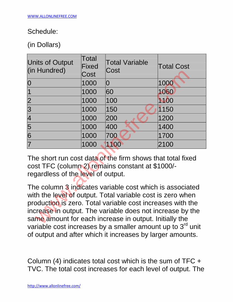
WWW.ALLONLINEFREE.COM
http://www.allonlinefree.com/
Schedule:
(in Dollars)
Units of Output (in Hundred)
Total Fixed Cost
Total Variable Cost
Total Cost
0 1000 0 1000
1 1000 60 1060
2 1000 100 1100
3 1000 150 1150
4 1000 200 1200
5 1000 400 1400
6 1000 700 1700
7 1000 1100 2100
The short run cost data of the firm shows that total fixed cost TFC (column 2) remains constant at $1000/- regardless of the level of output.
The column 3 indicates variable cost which is associated with the level of output. Total variable cost is zero when production is zero. Total variable cost increases with the increase in output. The variable does not increase by the same amount for each increase in output. Initially the variable cost increases by a smaller amount up to 3
rd unit
of output and after which it increases by larger amounts.
Column (4) indicates total cost which is the sum of TFC + TVC. The total cost increases for each level of output. The
www.allo
nline
free.
com

WWW.ALLONLINEFREE.COM
http://www.allonlinefree.com/
rise in total cost is more sharp after the 4th level of output.
The concepts of costs, i.e., (1) total fixed cost (2) total variable cost and (3) total cost can be illustrated graphically.
(i) Total Fixed Cost Curve/Diagram:
In this diagram (13.1) the total fixed cost of a firm is assumed to be $1000 at various levels of output. It remains the same even if the firm's output is zero.
(ii) Total Variable Cost Curve/Diagram:
In the figure (13.2), the total variable cost curve (TVC) increases with the higher level of output. It starts from the origin. Then increases at a diminishing rate up to the 4th units of output. It then begins to rise at an increasing rate.
Total Cost Curve Curve/Diagram:
www.allo
nline
free.
com

WWW.ALLONLINEFREE.COM
http://www.allonlinefree.com/
In the figure (13.3), total cost curve which is the sum of the total fixed cost and variable cost at various levels of output has nearly the same shape. The difference between the two is by only a fixed amount of $1,000. The total variable cost curve and the total cost curve begin to rise more rapidly as production is increased. The reason for this is that after a certain
output, the business has passed its most efficient use of its fixed costs machinery, building etc., and its diminishing return begins to set in.
Analytical Importance of Fixed and Variable Costs:
In the time of distinction between fixed cost and variable cost is a matter of degree, it all depends upon the contracts of a firm and .the period of time under consideration.
For example, if a firm makes contract with the labor for a certain period, then the firm has to bear the cost of the labor irrespective of the total produce. Under such conditions, the wages paid to the labor will be classified as fixed cost and not variable cost, as discussed under the heading of variable cost. Secondly, when the period of
www.allo
nline
free.
com

WWW.ALLONLINEFREE.COM
http://www.allonlinefree.com/
time is short, the distinction between fixed cost and variable cost can be made rigid but not in a longer period of time all fixed costs change into variable cost in the long run.
Average Cost:
Definition and Explanation:
The entrepreneurs are no doubt interested in the total costs but they are equally concerned in knowing the cost per unit of the product. The unit cost figures can be derived from the total fixed cost, total variable cost and total cost by dividing each of them with corresponding output.
Types/Classifications:
(1) Average Fixed Cost (AFC):
Average fixed cost refers to fixed cost per unit of output. Average fixed Cost is found out by dividing the total fixed cost by the corresponding output.
Formula:
AFC = TFC
Output (Q)
For instance, if the total fixed cost of a shoes factory is $5,000 and it produces 500 pairs of shoes, then the average fixed cost is equal to $10 per unit. If it produces 1,000 pairs of shoes, the average fixed cost is $5 and if
www.allo
nline
free.
com

WWW.ALLONLINEFREE.COM
http://www.allonlinefree.com/
the total output is 5,000 pairs of shoes, then the average fixed cost is $1 pair of shoe.
From the above example, it is clear, that the fixed cost, i.e., $5,000 remains the same whether the output is 1,000 or 5,000 units.
Behavior of Average Fixed Cost (AFC):
The average fixed cost begins to fall with the increase in the number of units produced, In our example stated above, average fixed cost in the beginning was $10. As the output of the firm increased, it gradually came down to $1. The AFC diminishes with every increase in the quantity of output produced but it never becomes zero.
Diagram/Curve:
The concept of average fixed cost can be explained with the help of the curve, in the diagram (13.4) the average fixed cost curve gradually falls from left to right showing the level of output. The larger the level of output, the lower is the average fixed cost and smaller the level of output, the greater is the average fixed cost. The AFC never
www.allo
nline
free.
com

WWW.ALLONLINEFREE.COM
http://www.allonlinefree.com/
becomes zero.
(2) Average Variable Cost (AVC):
Average variable cost refers to the variable expenses per unit of output Average variable cost is obtained by dividing the total variable cost by the total output.
For instance, the total variable cost for producing 100 meters of cloth is $800, the average variable cost will be $8 per meter.
Formula:
AVC = TVC
(Q)
Behavior of Average Variable Cost:
When a firm increases its output, the average variable cost decreases in the beginning, reaches a minimum and then increases. Here, a question can be asked as to why AVC decreases in the beginning reaches a minimum and then increases. The answer to this question is very simple.
When in the beginning, a firm is not producing to its full capacity, then the various factors of production employed for the manufacture of a particular commodity remain partially absorbed. As the output of the firm is increased, they are used to its fullest extent. So the AVC begins to decrease. When the plant works to its full capacity, the
www.allo
nline
free.
com

WWW.ALLONLINEFREE.COM
http://www.allonlinefree.com/
AVC is at its minimum. If the production is pushed further from the plant capacity, then less efficient machinery and less, efficient labour may have to be employed. This results in the rise of AVC. It is in this way we say that as the output of a firm increases, the AVC decreases in the beginning, reaches a minimum and then increases. The AVC can also be represented in the form of a curve.
Diagram/Curve:
The shape of the average variable cost curve (Fig. 13.5) is like a flat U-shaped curve. It shows that when the output is increased, there is a steady fall in the average variable cost due to increasing returns to variable factor. It is minimum when 500 meters of doth are produced. When production is increased to 600 meters, of cloth or more, the average variable cost begins to increase due to diminishing returns to the variable factor.
(3) Average Total Cost (ATC):
Average total cost refers to cost (both fixed and variable) per unit of output. Average total cost is obtained by dividing the total cost by the total number of commodities produced by the firm or when the total sum of average variable cost and average fixed cost is added together, it
www.allo
nline
free.
com

WWW.ALLONLINEFREE.COM
http://www.allonlinefree.com/
becomes equal to average total cost.
Formula:
ATC = Total Cost (TC)
Output (Q)
Behavior of Average Total Cost:
As the output of a firm increases, average total cost like the average variable cost decreases in the beginning reaches a minimum and then it increases. The reasons for decline of ATC in the beginning are that it is the sum of AFC and AVC.
Average fixed cost and average variable costs have both the tendency to fall as output is increased. Average total cost will continue falling so long average variable cost does not rise. Even if average variable cost continues rising, it is not necessary that the average total cost will rise. It can be due to the fact that the increase in average variable cost is less than the fall in average fixed cost. The increase in average variable cost is counterbalanced by a rapid fall of average fixed cost. If the rise in the average variable cost is greater than the fall in average fixed cost, then the average total cost will rise.
The tendency to rise on the part of average total cost-in the beginning is slow, after a certain point it begins to increase rapidly.
www.allo
nline
free.
com

WWW.ALLONLINEFREE.COM
http://www.allonlinefree.com/
Diagram/Curve:
The average total cost is represented here by a shaped curve in Fig. (13.6). The average total cost curve is also like a U-shaped curve. It shows that as production increases from 100 meters to 200 meters of cloth, the cost falls rapidly, reaches a minimum but then with higher level of output, the average fixed cost begins to increase.
Short Run and Long Run Average Cost Curves:
Relationship and Difference:
Short Run Average Cost Curve:
In the short run, the shape of the average total cost curve (ATC) is U-shaped. The, short run average cost curve falls in the beginning, reaches a minimum and then begins to rise. The reasons for the average cost to fall in the beginning of production are that the fixed factors of a firm remain the same. The change only takes place in the variable factors such as raw material, labor, etc.
As the fixed cost gets distributed over the output as production is expanded, the average cost, therefore, begins to fall. When a firm fully utilizes its scale of
www.allo
nline
free.
com

WWW.ALLONLINEFREE.COM
http://www.allonlinefree.com/
operation (plant size), the average cost is then at its minimum. The firm is then operating to its optimum capacity. If a firm in the short-run increases its level of output with the same fixed plant; the economies of that scale of production change into diseconomies and the average cost then begins to rise sharply.
Long Run Average Cost Curve:
In the long run, all costs of a firm are variable. The factors of production can be used in varying proportions to deal with an increased output. The firm having time-period long enough can build larger scale or type of plant to produce the anticipated output. The shape of the long run average cost curve is also U-shaped but is flatter that the short run curve as is illustrated in the following diagram:
Diagram/Figure:
In the diagram 13.7 given above, there are five alternative scales of plant SAC
1 SAC
2, SAC
3, SAC
4 and, SAC
5. In the
long run, the firm will operate the scale of plant which is most profitable to it.
www.allo
nline
free.
com

WWW.ALLONLINEFREE.COM
http://www.allonlinefree.com/
For example, if the anticipated rate of output is 200 units per unit of time, the firm will choose the smallest plant It will build the scale of plant given by SAC
1 and operate it at
point A. This is because of the fact that at the output of 200 units, the cost per unit is lowest with the plant size 1 which is the smallest of all the four plants. In case, the volume of sales expands to 400, units, the size of the plant will be increased and the desired output will be attained by the scale of plant represented by SAC
2 at point B, If the
anticipated output rate is 600 units, the firm will build the size of plant given by SAC
3 and operate it at point C where
the average cost is $26 and also the lowest The optimum output of the firm is obtained at point C on the medium size plant SAC
3.
If the anticipated output rate is 1000 per unit of time the firm would build the scale of plant given by SAC
5 and
operate it at point E. If we draw a tangent to each of the short run cost curves, we get the long average cost (LAC) curve. The LAC is U-shaped but is flatter than tile short run cost curves. Mathematically expressed, the long-run average cost curve is the envelope of the SAC curves.
In this figure 13.7, the long-run average cost curve of the firm is lowest at point C. CM is the minimum cost at which optimum output OM can be, obtained.
Marginal Cost (MC):
Definition:
www.allo
nline
free.
com

WWW.ALLONLINEFREE.COM
http://www.allonlinefree.com/
Marginal Cost is an increase in total cost that results from a one unit increase in output. It is defined as:
"The cost that results from a one unit change in the production rate".
Example:
For example, the total cost of producing one pen is $5 and the total cost of producing two pens is $9, then the marginal cost of expanding output by one unit is $4 only (9 - 5 = 4).
The marginal cost of the second unit is the difference between the total cost of the second unit and total cost of the first unit. The marginal cost of the 5th unit is $5. It is the difference between the total cost of the 6th unit and the total cost of the, 5th unit and so forth.
Marginal Cost is governed only by variable cost which changes with changes in output. Marginal cost which is really an incremental cost can be expressed in symbols.
Formula:
Marginal Cost = Change in Total Cost = ΔTC
Change in Output Δq
The readers can easily understand from the table given below as to how the marginal cost is computed:
www.allo
nline
free.
com

WWW.ALLONLINEFREE.COM
http://www.allonlinefree.com/
Schedule:
Units of Output Total Cost (Dollars) Marginal Cost (Dollars)
1 5 5
2 9 4
3 12 3
4 16 4
5 21 5
6 29 8
Graph/Diagram:
MC curve, can also be plotted graphically. The marginal cost curve in fig. (13.8) decreases sharply with smaller Q output and reaches a minimum. As production is expanded to a higher level, it begins to rise at a rapid rate.
Long Run Marginal Cost Curve:
The long run marginal cost curve like the long run average cost curve is U-shaped. As production expands, the marginal cost falls sharply in the beginning, reaches a minimum and then rises sharply.
Relationship Between Log Run Average Cost and
www.allo
nline
free.
com

WWW.ALLONLINEFREE.COM
http://www.allonlinefree.com/
Marginal Cost:
The relationship between the long run average total cost and log run marginal cost can be understood better with
the help of following diagram:
It is clear from the diagram (13.9), that the long run marginal cost curve and the long run average total cost curve show the same behavior as the short run marginal cost curve express with the short run average total cost curve. So long as the average cost curve is falling with the increase in output, the marginal cost curve lies below the average cost curve.
When average total cost curve begins to rise, marginal cost curve also rises, passes through the minimum point of the average cost and then rises. The only difference between the short run and long run marginal cost and average cost is that in the short run, the fall and rise of curves LRMC is sharp. Whereas In the long run, the cost curves falls and rises steadily.
PRICING UNDER PERFECT COMPETITION
Market Structure:
Definition of Market:
A market is a set of conditions in which buyers and sellers meet each other for the purpose of exchange of goods
www.allo
nline
free.
com

WWW.ALLONLINEFREE.COM
http://www.allonlinefree.com/
and services for money.
Elements of Market:
The essentials of a market are:
(i) Presence of goods and services to be exchanged.
(ii) Existence of one or more buyers and sellers.
(iii) A place or a region where buyers and sellers of a good get in close touch with each other.
Types of Market/Market Model:
Markets are classified according to the number of firms in the market and by the commodity to be exchanged. The economists on the basis of variation in the features of market describe four market models:
(i) Perfect Competition.
(ii) Pure Monopoly.
(iii) Monopolistic Competition.
(iv) Oligopoly.
In the analysis of each market model, it is examined as to what determines the equilibrium price, output and profit levels for the individual firm and for the industry, in this chapter, we discuss the most important of the various market models that is perfect competition.
www.allo
nline
free.
com

WWW.ALLONLINEFREE.COM
http://www.allonlinefree.com/
PERFECT COMPETITION
Definition:
The concept of perfect competition was first introduced by Adam Smith in his book "Wealth of Nations". Later on, it was improved by Edgeworth. However, it received its complete formation in Frank Kight's book "Risk, Uncertainty and Profit" (1921).
Leftwitch has defined market competition in the following words:
"Prefect competition is a market in which there are many firms selling identical products with no firm large enough, relative to the entire market, to be able to influence market price".
According to Bllas:
"The perfect competition is characterized by the presence of many firms. They sell identically the same product. The seller is a price taker".
The main conditions or features of perfect competition are as under:
Features/Characteristics or Conditions:
(1) Large number of firms. The basic condition of perfect competition is that there are large number of firms in an industry. Each firm in the industry is so small and its output so negligible that it exercises little influence over price of the commodity in the market. A single firm cannot
www.allo
nline
free.
com

WWW.ALLONLINEFREE.COM
http://www.allonlinefree.com/
influence the price of the product either by reducing or increasing its output. An individual firm takes the market price as given and adjusts its output accordingly. In a competitive market, supply and demand determine market price. The firm is price taker and output adjuster.
(2) Large number of buyers. In a perfect competitive market, there are very large number of buyers of the product. If any consumer purchases more or purchases less, he is not in a position to affect the market price of the commodity. His purchase in the total output is just like a drop in the ocean. He, therefore, too like the firm, is a price taker.
(3) The product is homogeneous. Another provision of perfect competition is that the good produced by all the firms in the industry is identical. In the eyes, of the consumer, the product of one firm (seller) is identical to that of another seller. The buyers are indifferent as to the firms from which they purchase. In other words, the cross elasticity between the products of the firm is infinite.
(4) No barriers to entry. The firms in a competitive market have complete freedom of entering into the market or leaving the industry as and when they desire. There are no legal, social or technological! barriers for the new firms (or new capital) to enter or leave the industry. Any new firm is free to start production if it so desires and stop production and leave the industry if it so wishes. The industry, thus, is characterized by freedom of entry and exit of firms.
www.allo
nline
free.
com

WWW.ALLONLINEFREE.COM
http://www.allonlinefree.com/
(5) Complete information. Another condition for perfect competition is that the consumers and producers possess perfect information about the prevailing price of the product in the market. The consumers know the ruling price, the producers know costs, the workers know about wage rates and so on. In brief, the consumers, the resource owners have perfect knowledge about the current price of the product in the market. A firm, therefore, cannot charge higher price than that ruling in the market. If it does so, its goods will remain unsold as buyers will shift to some other seller.
(6) Profit maximization. For perfect competition to exist, the sole objective of the firm must be to get maximum profit.
Equilibrium of the Firm Under Perfect Competition orMarginal Revenue = Marginal Cost (MR = MC) Rule:
Definition and Explanation:
A firm under perfect competition faces an infinitely elastic demand curve or we can say for an individual firm, the price of the commodity is given in the market. The firm while making changes in the amounts of variable factor evaluates the extra cost incurred on producing extra unit MC (Marginal Cost).
It also examines the change in total receipts which results from the sale of extra unit of production MR (Marginal Revenue). So long as the additional revenue from the sale
www.allo
nline
free.
com

WWW.ALLONLINEFREE.COM
http://www.allonlinefree.com/
of an extra unit of product (MR) is greater than the additional cost (MC) which a firm has to incur on its production, it will be in the interest of the firm to increase production.
In economic terminology, we can say, a firm will go on expanding its output so long as the marginal revenue of any unit is greater than its marginal cost. As production increases, marginal cost begins to increase after a certain point. When both marginal revenue and marginal cost are equal, the firm is in equilibrium. The firm at this equilibrium point is cither ensuring maximum profit or minimizing losses. This is shown with the help of a diagram below:
Diagram/Figure:
In the figure (15.2) quantity of output is measured along OX axis and marginal cost and marginal revenue on OY axis. The marginal cost curve cuts the marginal revenue curve at two points K and T.
The competitive firm is in equilibrium, at both these points as marginal cost equals marginal revenue. The firm will not produce OM quantity of good because for OM output,
www.allo
nline
free.
com

WWW.ALLONLINEFREE.COM
http://www.allonlinefree.com/
the marginal cost is higher than marginal revenue. Marginal cost curve cuts the marginal revenue curve from above. The firm incurs loss equal to the black shaded area for producing 50 units (OM) of output.
As production is increased from 50 units to 350 units (from OM to OS) marginal cost decreases at early levels of output and then increases thereafter. The marginal cost curve cuts the marginal revenue curve from below at point T. The shaded portion between M to S level of output shows profit on production. When a firm produces OS quantity of output; it earns maximum profit. The point T where MR = MC is the point of maximum profit.
In case, the firm increases the level of output from OS, the additional output adds less to Its revenue than to its cost. The firm undergoes losses as is shown in the shaded area.
Summing up, profit maximization normally occurs at the rate of output at which marginal revenue equals marginal cost. This golden rule holds good for all market structures. As regards the absolute profits and losses of the firm, they depend upon the relation between average cost and average revenue of the firm.
Short Run Equilibrium of the Price Taker Firm Under Perfect Competition:
Definition and Explanation:
By short run is meant a length of time which is not enough to change the level of fixed inputs or the number of firms in
www.allo
nline
free.
com
WWW.ALLONLINEFREE.COM
http://www.allonlinefree.com/
the industry but long enough to change the level of output by changing variable inputs.
In short period, a distinction is made of two types of costs (i) fixed cost and (ii) variable cost.
The fixed cost in the form of fixed factors i.e., plant, machinery, building, etc. does not vary with the change in the output of the firm. If the firm is to increase or decrease its output, the change only takes place in the quantity of variable resources such as labor, raw material, etc.
Further, in the short run, the demand curve facing the firm is horizontal. No new firms enter or leave the industry. The number of firms in the industry, therefore, remain the same. Under perfect competition, the firm takes the price of the product as determined in the market. The firm sells all its output at the prevailing market price. The firm, in other words, is a price taker.
Equilibrium of a Competitive Firm:
The short-run equilibrium of a firm can be easily explained with the help of marginal revenue = marginal cost approach or (MR = MC) rule.
Marginal revenue is the change in total revenue that occurs in response to a one unit change in the quantity sold. Marginal cost is the addition to total cost resulting from the additional of marginal unit. Since price is given for the competitive firm, the average revenue curve of a price taker firm is identical to the marginal curve. Average revenue (AR) thus is equal to marginal revenue (MR) is
www.allo
nline
free.
com

WWW.ALLONLINEFREE.COM
http://www.allonlinefree.com/
equal to price (MR = AR = Price).
According to the marginal revenue and marginal cost approach or (MR = MC) rule , a price taker firm is in equilibrium at a point where marginal revenue (MR) or price is equal to marginal cost The point where MR = MC = Price, the firm produces the best level of output. From this it may not be concluded that the perfectly competitive firm at the equilibrium level of output (MR = MC = Price) necessarily ensures maximum profit. The fact is that in the short period, a firm at the equilibrium level of output is faced with four types of product prices in the market which give rise to following results:
(i) A firm earns supernormal profits.
(ii) A firm earns normal profits.
(iii) A firm incurs losses but does not close down.
(iv) A firm minimizes losses by shutting down. All these short run cases of profits or losses are explained with the help of diagrams.
Short Run Supply Curve of a Price Taker Firm:
Definition and Explanation:In a competitive market, the supply curve of a firm is derived from its marginal cost curve. Supply curve is that portion of the marginal cost curve which lies above the average variable cost curve.
As we already know, the aim of the firm is to maximize profits or minimize losses. The profits are increased it the
www.allo
nline
free.
com

WWW.ALLONLINEFREE.COM
http://www.allonlinefree.com/
difference between total receipts and total costs is maximized. When a firm undertakes the production of a particular commodity, it has to pay remuneration to all the factors of production employed. The remuneration or cost of the firm for a short period can be divided into two parts, fixed costs and variable costs. If from the sale of the commodity produced, a firm is earning much more than what it has to spend on it. We say a firm is earning abnormal profits if the total revenue of the firm is equal to total cost, the firm is getting normal profits. In both these cases, it is profitable for the firm to produce the commodity. But if the total receipts fall short of total costs, then three situations can arise.
(i) A firm is not in position to meet its variable costs.
(ii) A firm is able to cover its variable costs.
(iii) A firm is covering its full variable costs and a part of the fixed costs.
Let us explain all these situations with the help of a curve.
Diagram:
www.allo
nline
free.
com

WWW.ALLONLINEFREE.COM
http://www.allonlinefree.com/
Summing up, we can say, that if price falls below the lowest point on the AVC curve, the firm will not produce any output because it is not able to cover even its total variable costs. But if the price is such that it covers its total variable costs, then the firm may carry on production for a short period. So is also the case when it covers its full variable costs and a part of the fixed costs. In the long period, if the firm does not cover its full costs, it will have to dose down its operations sooner or later. So we conclude that the supply curve of the firm that can be regarded as that portion of the MC curve which lies above the AVC curve and not which lies below the AVC curve because it is only at the lowest point on the AVC curve that some output is forthcoming and not below this point.
The supply curve of the firm or the rising portion of the MC curve which lies above the AVC curve can be split up into two parts. One part consists of that portion which lies above the lowest point of the ATC curve. If the price line representing MR = AR intersects the MC curve at any point on this rising portion, the firm will be earning abnormal profit (see fig. 15.7). The second part of the supply curve of the firm extends from the lowest point of
www.allo
nline
free.
com

WWW.ALLONLINEFREE.COM
http://www.allonlinefree.com/
the AVC curve to the lowest, point of the ATC curve. If price line representing MR = AR passes through the lowest point of the AVC curve, the firm is covering only total variable costs. If the price line cuts the MC curve at any point above the lowest point of the AVC curve and below the lowest point of ATC curve, the firm will be meeting its total variable costs and a part of the fixed costs but not the total costs. The total costs are met only when the price line forms a tangent to the ATC curve.
Short Run Supply Curve of the Industry:
Definition:
The short run supply curve of a competitive firm is that part of the marginal cost curve which lies above the average variable cost. As regards industry supply curve, it is the horizontal summation of the short run supply carves of the identical firms constituting an industry.
Explanation:
The industry short run supply curve is briefly explained with the help of the diagram (15.8) below.
We assume here that prices of inputs do not change with the change in the size of the firm; However, when all firms increase or decrease output, the factor prices rise or fall respectively.
www.allo
nline
free.
com

WWW.ALLONLINEFREE.COM
http://www.allonlinefree.com/
Diagram:
In figure 15.8(a), we assume that at point P, price or marginal revenue equals marginal cost. The firm at equilibrium point P. ($4) produces and sells 50 units of a commodity. If the equilibrium of MR, MC, price occurs at point K, the firm produces and sells 100 units.
In figure 15.8(b), let us suppose that there are 100 firms in the industry. As all the firms by assumptions, have identical costs, the industry will be producing 5000 units at a market price of ($4) and 10000 units at industrial price of ($8). The industry supply curve, therefore, has a positive
www.allo
nline
free.
com

WWW.ALLONLINEFREE.COM
http://www.allonlinefree.com/
slope.
Long Run Equilibrium of the Price Taker Firm:
Definition:
"All the firms in a competitive industry achieve long run equilibrium when market price or marginal revenueequals marginal cost equals minimum of average total cost."
Formula:
Price = Marginal Cost = Minimum Average Total Cost
Explanation:
The long run is a period of time during which the firms are able to adjust their outputs according to the changing conditions. If the demand for a product increases, all the firms have sufficient time to expand their plant capacities, train and engage more labor, use more raw material, replace old machines, purchase new equipments, etc., etc.
If the demand for a product declines, the firms reduce the number of workers on the pay roll, use less raw material. In short, all inputs used by a firm are variable in the long run. It is assumed that all the firms in the competitive industry are producing homogeneous product and an individual firm cannot affect the market price. It takes the market price as given. It is also assumed that all the firms in a competitive industry have identical cost' curves. The
www.allo
nline
free.
com

WWW.ALLONLINEFREE.COM
http://www.allonlinefree.com/
industry it is assumed is, a constant cost industry. In the long run, it is for further assumed that all the firms in a competitive industry have access to the same technology.
When the period is long and profit level of the competitive industry is high, then new firms enter the industry. If the profit level is below the competitive level, the firm then leave the industry. When all the competitive firms earn normal profit, then there is no tendency for the new firms to enter or leave the industry. The firms are then in the long run equilibrium.
Diagram:
The case of long-run equilibrium of a firm can be easily explained with .the help of a diagram given below:
Long Run Supply Curve for the Industry:
Definition and Explanation:
www.allo
nline
free.
com

WWW.ALLONLINEFREE.COM
http://www.allonlinefree.com/
While explaining the short run supply curve for the firm, we stated that the supply curve in the short run is that portion of the marginal cost curve which lies above the average variable cost curve, it is because of the fact that when the variable casts of a firm are realized, the firm decides to produce the goods. In the short run, the firm is in equilibrium when the MR is equal to MC and both are equal to price. If this equilibrium takes place at the level above the minimum point of ATC curve, the firm is earning abnormal profits and if it is below the minimum point of ATC, then it is suffering losses. In the long run, a firm cannot operate at a loss, however small it may be.
The firm also cannot earn abnormal profits because in that case new firms enter into the industry. The supply of the goods increases in the market and price comes down to the level of normal price. In case of fall in demand, the capacity of the existing firms is contracted, old firms also withdraw from the industry and thus supply is automatically adjusted to demand. The firm, In the long run, is in equilibrium when price = marginal revenue = marginal cost = average total cost of the firm at the lowest point. When all the firms producing a single commodity are in equilibrium, the industry is in full equilibrium. Each firm in the industry is earning only normal profits.
The short run supply curve of the industry is derived as stated earlier by the lateral summation of that part of the marginal cost curves of all the firms which lie above the minimum point on the AVC curves. The long run supply curve, however, cannot be obtained by this method
www.allo
nline
free.
com

WWW.ALLONLINEFREE.COM
http://www.allonlinefree.com/
because in the long run the variations is demand produce long run adjustments in the output and also in the costs of productions of these firms. The changes in output take place because of the (1) greater or leaser production by the existing firms, (2) entry of new firms in the industry or withdrawals of old firms and (3) the emergence of external economies and diseconomies.
The emergence of external economies and diseconomies has a very important bearing on the shape of the long run supply curve. When an industry in the long run expands its size for greater production, it enjoys certain external economies such as (1) technical economies, (2) managerial economies (3) communications economies, (4) financial economies and (5) risk bearing economies. Internal economies may also arise out of the marketing facilities enjoyed by the firms in the purchase of raw material (6) in securing special concessional transport rates, etc., etc. The internal economies also lead to reduction in cost.
(1) If the size of the firm is expanded continuously, it meets diseconomies as well. For instance, co-ordination and organization of factors become difficult (2) capital may not be available in the required quantity (3) entrepreneurial inertia also stands in the way of expansion of the industry (4) the prices of raw material also increase due to greater demand by ail firms (5) the productivity of the additional factors may also be less. The appearances of these diseconomies result in increasing the marginal cost and average total cost of the firms to the higher levels. If the
www.allo
nline
free.
com

WWW.ALLONLINEFREE.COM
http://www.allonlinefree.com/
economies and diseconomies cancel each other, the industry wilt experience constant cost in the long run.
We, therefore conclude that the shape of the supply curve of the industry, depends upon the behavior of the cost in the long run.
Behavior of the Cost:
(1) If the industry is subject to constant cost, the shape of the supply curve will be perfectly elastic, i.e. it will be horizontal straight line parallel to the X-axis.
(2) If the industry obeys the taw of increasing cost or diminishing return, the shape of the supply curve will be positive, i.e. it will rise from left to right.
(3) If the industry is governed by the law of diminishing cost or increasing return, the long run supply curve will be negative, i.e., it will fall downward from left to right.
(1) Supply Curve of a Constant Cost Industry:
Diagram:
In figure 15.10(a) the firm is in the long-run equilibrium at
www.allo
nline
free.
com

WWW.ALLONLINEFREE.COM
http://www.allonlinefree.com/
point N where:
Price = MC = Minimum Average Cost
The firm produces output OP and sells at price OK per unit The firm like all other firms in the industry make normal profits. In figure 15.10(b), it is shown that when the market demand for .a product increases, the demand curve DD
/ shifts upwards. The new firms enter the industry and
each firm produces at its minimum point of average cost which is OK. The industry is thus producing any quantity of output at a price of OK. The supply curve of the industry is perfectly elastic at a price OK in the long run.
(2) Supply Curve of the Increasing Cost Industry:
Diagram:
In the figure 15.11(a) it is shown that when the demand for a commodity increases, more firms enter into the industry. In order to attract more units of the factors, the firms pay higher prices for them. The cost curves of the firms, move up. The minimum average cost of the firm equals marginal cost equals price at point F. The firm in the long run is in equilibrium at point F and produce the best level of output
www.allo
nline
free.
com

WWW.ALLONLINEFREE.COM
http://www.allonlinefree.com/
OT.
When the costs of the firms rise with the expansion of output, the supply 'curve of the industry Fig. 15.11(b) also slants upward. The industry is now in equilibrium at point R, with industry output OT and Price OK.
(3) Supply Curve of a Decreasing Cost Industry:
Diagram:
In the Fig. (15.12) the firm is in equilibrium at point K in the long run because at point K, MR = MC = Price = Minimum AC. It will produce OT output at price ON. The total supply by all the firms (supply of industry) producing the commodity at price ON will be OH. If the demand for the product increases, the existing firms will expand their sizes and the new firms will enter the industry/Due to
www.allo
nline
free.
com

WWW.ALLONLINEFREE.COM
http://www.allonlinefree.com/
technological developments and the economies of large scale production, the MC, AC, and price fall. At the lower price OP, the firm is in equilibrium at point F. Here MC = AC = Price. The supply of a firm increases from OT to OH at a decreasing cost. The supply of the industry at lower price OP increases from OH to OK. The long run equilibrium supply curve slopes downward from left to right.
PRICING UNDER MONOPOLY
What is Monopoly?
Definition and Meaning:
Monopoly is from the Greek word meaning one seller. It is the polar opposite of perfect competition. Monopoly is a market structure in which one firm makes up the entire market. Monopoly and competition are at the two extremes. It is define as:
"Monopoly refers to a market where there is a single seller for a product and there is no close substitute of the commodity that is offered by the sole supplier to the buyers. The firm constitutes the entire industry".
Explanation:
Monopoly, therefore, indicates a case where:
(i) There is only a single seller of a product or service in the market.
(ii) The goods produced by a sole seller has not close
www.allo
nline
free.
com

WWW.ALLONLINEFREE.COM
http://www.allonlinefree.com/
substitutes.
(iii) The entry of new firms into the industry is effectively barred by legal or natural barriers.
(iv) The firm being the sole supplier of a product constitutes industry. Firm and industry thus have single identity. Or we can say monopoly is a single firm identity.
(v) The single seller affects no other seller by its own action in the market. The other sellers too cannot affect the price and output of the monopolist.
(vi) The demand curve facing the monopolist is negatively sloped. The monopolist being the only seller of the commodity in the market can increase the total sale by lowering the price and if, he raises the price, he would not lose all his sale. The demand curve facing a monopolist is less than perfectly elastic, i.e., . it slopes downward from left to right.
For the monopoly to exist, it is not necessary that the size of a firm should .be large. Even a small firm may have a monopoly. For instance, a local water company or a local electricity company, supplying water and electricity in the city possesses all the characteristics of a monopoly.
www.allo
nline
free.
com

WWW.ALLONLINEFREE.COM
http://www.allonlinefree.com/
Short Run Equilibrium Price and Output Under Monopoly:
Short Run Equilibrium of the Monopoly Firm:
In the short period, the monopolist behaves like any other firm. A monopolist will maximize profit or minimize losses by producing that output for which marginal cost (MC) equals marginal revenue (MR). Whether a profit or loss is made or not depends upon the relation between price and average total cost (ATC). It may be made clear here that a monopolist does not necessarily makes profit. He may earn super profit or normal profit or even produce at a loss in the short ran.
Conditions for the Equilibrium of a Monopoly Firm:
There are two basic conditions for the equilibrium of the monopoly firm.
First Order Condition: MC = MR.
Second Order Condition: MC curve cuts MR curve from below.
Explanation:
(a) Short Run Monopoly Equilibrium With Positive Profit:
In the short period, if the demand for the product is high, a monopolist increase the price and the quantity of output. He can increase the, output by hiring more labor, using more raw material, increasing working hours etc. However, he cannot change his fixed plant and equipment. In case, the demand for the product falls, he
www.allo
nline
free.
com

WWW.ALLONLINEFREE.COM
http://www.allonlinefree.com/
then decreases the use of variable inputs, (like labor, material etc.).
b) Short Run Equilibrium With Normal Profit Under Monopoly:
There is a false impression regarding the powers of a monopolist. It is said that the monopolistic entrepreneur always earns profits. The fact, however, is that there is no guarantee for the monopolist to earn profit in the short run. If a monopolist firm produces a new commodity and attempts to change the taste pattern of the consumers through advertising campaigns etc., then the firm may operate at normal profit or even produce at a loss minimizing price in the short run (Covering variable cost only).
(c) Short Run Equilibrium With Losses Under Monopoly:
A monopolist also accepts short run losses provided the variable costs of the firm are fully covered.
Long Run Equilibrium Under Monopoly:
The monopolist creates barriers of entry for the new firms into the industry. The entry into the industry is blocked by having control over the raw materials needed for the production of goods or he may hold full rights to the production of a certain good (patent) or the market of the good may be limited. If new firms try to enter in the field, it lowers the price of the good to such on extent that it becomes unprofitable for new firms to continue production
www.allo
nline
free.
com

WWW.ALLONLINEFREE.COM
http://www.allonlinefree.com/
etc.
When there is no threat of the entry of new firms into the industry, the monopoly firm makes long run adjustments in the scale of plant. In case, the demand for the product is limited, the monopolist can afford to produce output at sub optimum scale. If the market size is large and permits to expand output, then the monopolist would build an optimum scale of plant and would produce goods at the minimum cost per unit. However, the monopolist would not stay in the business, if he makes losses in the long period. The long run equilibrium of a monopoly firm is now explained with the help of the following diagram.
Diagram/Curve:
In the long run, all the factors of production including the size of the plant are variable. A monopoly firm will maximize profit at that level of output for which long run marginal cost (MC) is equal to marginal revenue (MR) and the LMC curve intersects the MR curve from below. In the
www.allo
nline
free.
com

WWW.ALLONLINEFREE.COM
http://www.allonlinefree.com/
figure (16.6), the monopoly firm is in equilibrium at point E where LMC = MR and LMC cuts MR curve from below. QP is the equilibrium price and OQ is the equilibrium output.
Monopoly Price Discrimination:
What is Price Discrimination?
While discussing price determination under monopoly, it was assumed that a monopolist charges only one price for his product from all the customers in the market. But it often so happens that a monopolist, by virtue of his monopolistic position, may manage to sell the same commodity at different prices to different customers or in different markets. The practice on the part of the monopolist to sell the identical goods at the same time to different buyers at different prices when the price difference is not Justified by difference in costs in calledprice discrimination. In the words of Mrs. Joan Robinson:
"Price discrimination is the act of selling the same article produced under single control at a different prices to the different buyers".
Types and Examples of Price Discrimination:
Price discrimination may be of various types. It may either be (i) personal (ii) trade discrimination (iii) local discrimination.
(1) Price discrimination. It is persona!, when separate price is charged from each buyer according to the intensity
www.allo
nline
free.
com

WWW.ALLONLINEFREE.COM
http://www.allonlinefree.com/
of his desire or according to the size of his pocket.
For instance, a doctor may charge $20000 from a rich person for an eye operation and $500 only from a poor man for the similar operation.
(2) Trade discrimination. It may take place when a monopolist charges different prices according to the uses to which the commodity is put. For example, an electricity company may charge low rate for electric current used in an industrial concern than for the electricity used for the domestic purpose.
(3) Place discrimination. It occurs when a monopolist charges different prices for the same commodity at different places. This type of discrimination is called dumping.
In Economics, a monopolist sells the same commodity at a higher price in one market and at a lower price in the other. Dumping may be undertaken due to several reasons, (a) a monopolist may resort to dumping in order to dispose off the accumulated stock or (b) he may, dump the commodity with a desire to capture the foreign market, (c) dumping may also be done to drive the competitors out of the market, (d) the motive may also be to reap. the economies of large scale production, etc.
PRICING UNDER MONOPOLISTIC COMPETITION
Definition:
Monopolistic/Imperfect competition as the name signifies
www.allo
nline
free.
com

WWW.ALLONLINEFREE.COM
http://www.allonlinefree.com/
is a blend of monopoly and competition. It is a systematic and realistic theory of price analysis in this imperfectly competitive world.
Monopolistic competition is a market situation in which there are relatively large number of small firms which produce or sell similar but not identical commodities to the customers.
According to Leftwitch:
"Monopolistic competition is a market situation in which there are many sellers of a particular product, but the product of each seller is in some way differentiated in the minds of consumers from the product of every other seller".
In the words of J.S. Bain:
"Monopolistic competition is found in the industry where there is a large number of small sellers selling differentiated but close substitute products".
Examples of Monopolistic Competition:
For example, a firm supplies branded good 'Lux Soap' in the market. There are many other firms in the market which sell similar soaps (not identical) with different brand names like Rexona, Palm Rose, etc., etc. The firm supplying 'Lux Soap' enjoys a monopoly position over the sale of its own product. It also faces competition from firms selling similar products.
www.allo
nline
free.
com

WWW.ALLONLINEFREE.COM
http://www.allonlinefree.com/
Same is the case with many other firms in the market like plywood manufacturing, jewellery making, wood furniture, book stores, departmental stores, repair services of all kinds, professional services of doctors, technicians, etc., etc. These firms and others which have an element of monopoly power and also face competition over the sale of product or service in the market are called monopolistically competitive firms.
Characteristics of Monopolistic/Imperfect Competition:
The main characteristic or features of monopolistic competition are as under:
(i) A fairly large number of sellers: The number of firms in monopolistic competition is fairly large. Each firm produces or sells a close substitute for the product of other firms in the product group or industry. .Product differentiation is thus the hallmark of monopolistic competition.
(ii) Differentiation in products: Under monopolistic competition, the firms sell differentiated products. Product differentiation may be real or imaginary. Real differentiation is done through differences in the materials used, design, color etc. Imaginary differences may be created through advertisement, brand name, trade marks etc. The firms producing similar products in .this imperfectly competitive world cannot raise the price of product much higher than their rivals. If they do so, they will lose much of their sale, but not all the sale. In case, they lower the price, the total sale can be increased to a
www.allo
nline
free.
com

WWW.ALLONLINEFREE.COM
http://www.allonlinefree.com/
certain extent. How much will the sale increase or decrease by lowering or raising the price will depend upon the product differentiation of the different firms.
If the product of the various firms are very close substitutes of one another and no imaginary or real difference exists in the mind of the buyers, then a slight rise or fall in the price of the product of one firm will appreciably decrease or increase the demand for the product. If the product of one firm differs from that of other firm, (though the difference may be an imaginary one) a slight rise in the price of the product of one firm will not drive away all its customers. A few faithless buyers may be attracted by the low price of the other rival product but not all the buyers.
(iii) Advertisement and propaganda: Another very important characteristic of the monopolistic competition is that each firm tries to create difference in its product from the other by advertising, propaganda, attractive packing, nice smile, etc., etc. When it succeeds in its object, the firm occupies almost the position of a monopolist. It is, thus, in a position to raise-the price of the product without losing its customers.
(iv) Nature of demand curve: Since the existence of close substitutes limits the monopoly power, the demand curve faced by a monopolistically competitive firm is fairly elastic. The precise degree of elasticity will however, depend upon the number of firms in the group product or industry. If the number of firms is fairly large and the product of each firm is not very similar, the demand curve
www.allo
nline
free.
com

WWW.ALLONLINEFREE.COM
http://www.allonlinefree.com/
of a firm will be quite elastic. In case, there is close competition among the rival firms for the sale of similar products, the demand curve of a firm will be less elastic.
(v) Freedom of entry and exit of firms: The entry of new firms in the monopolistically competition industry is relatively easy. There are no barriers of the new firm to enter the product group or leave the industry in the long run.
(vi) Sales efforts: With heterogeneous products, the sale of the products by the firms can no longer be taken for granted sale depends upon sale efforts.
(vii) Non-price competition: In monopolistic competition, the firms make every effort to win over the customers. Other than price cutting, the firms may offer after sale service, a gift scheme, discount not declared in the price list etc.
Equilibrium Price and Output in the Long Run Under Monopolistic/Imperfect Competition:
Long Run Zero Economic Profits:
In the long run, the firms are able to alter the scale of plant according to the changed conditions of demand for a product in the market. They can also leave or enter the industry. If the firms are earning abnormal profits in the short run, then new firm will enter the 'product group' (industry). The tendency of the new firms to enter the industry continues till the abnormal profits are competed away and the firms economic profits are zero. In case the
www.allo
nline
free.
com

WWW.ALLONLINEFREE.COM
http://www.allonlinefree.com/
monopolistically competitive firms realize losses in the short-run, then some of the firms will leave the industry. The exit of the firm continues till zero economic profits are restored with the operating firms.
In the long-run, there are no entry barriers for the new firms. The incoming firms install latest machinery and try to differentiate their products from those of the established firms. The old firms operating with .the used machinery try to match up with the new entrants by improved variety of products in their group. They increase expenditure on advertisement and on other sales promotional measures. They employ more qualified staff for. making technical improvement in their products. Since all the firms for their existence incur additional expenditure for improving the quality of the products, the cost curves of all the firms move up. Due to entry of new firms in the industry and higher costs of production, the output of each competing firm is reduced. There is, therefore, a waste in the economic resources of the country. The equilibrium price and output in the long-run is explained with the help of a diagram.
Diagram:
www.allo
nline
free.
com

WWW.ALLONLINEFREE.COM
http://www.allonlinefree.com/
In the figure (17.3), the higher shifted long-run marginal cost curve intersects the higher shifted marginal revenue curve at point M. The firm at this raised equilibrium point, produces the reduced level of output OK. It sells this output at price TK as at point T, LAC is a tangent to the demand or average revenue curve at its minimum point. The total revenue of the firm is equal to the area OETK. The total costs of the firm are also equal to the area OETK. The firm is earning only zero or normal economic profits. As the monopolistically competitive firm sets a price higher than that minimum average cost in the long-run, the firm therefore produces a smaller output. Since all the firms in the product group produce less at higher price, there is, therefore, an apparent waste of resources and exploitation of the consumers.
The advocates of monopolistic competition are of the opinion that if consumers get differentiated products at slightly higher prices (than with no choice under perfect competition), the consumers are then not exploited. There is no wasting of resources either, as the consumer's welfare increases with the product differentiation.
Short Run Equilibrium Under Monopolistic/Imperfect Competition:
Monopolistic competition refers to the market organization where there are a fairly large number of firms which sell somewhat differentiated products.
www.allo
nline
free.
com

WWW.ALLONLINEFREE.COM
http://www.allonlinefree.com/
A single firm in the product group (industry) has little impact on the market price. However, if it reduces price, it can expect a considerable increase in its sales. The firm may also attract buyers away from other firms by creating imaginary or real difference through advertising, branding and through many other sales promotion measures (non-price competition). If the firm raises its price, it will not lose all its customers. This is because of the fact that the product is differentiated from competing firms due to price and non-price factors. The demand curve (AR curve) of the monopolistic firm is therefore, highly elastic and is downward sloping. As regards the marginal revenue curve, it slopes downward and lies below the demand curve because price is lowered of all the units to sell more output in the market.
Firm's Equilibrium Price and Output:
In the short-run, the number of firms in the 'product group' remains the same. The size of the plant of each firm remains unaltered. The firm whether operating under perfect competition, or monopoly wants to maximize profits. In order to achieve this objective, it goes on producing a commodity so long as the marginal revenue is greater than marginal cost. When MR = MC, it is then in equilibrium and produces the best level of output. If a firm produces less than or more than the MR = MC output, it will then not be making maximum of profits.
In the short-run, a monopolistically competitive firm may be realizing abnormal profits or suffering losses. If it is earning profits, no new firms can enter the industry in the
www.allo
nline
free.
com
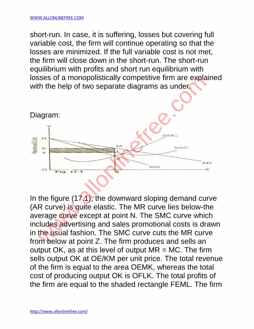
WWW.ALLONLINEFREE.COM
http://www.allonlinefree.com/
short-run. In case, it is suffering, losses but covering full variable cost, the firm will continue operating so that the losses are minimized. If the full variable cost is not met, the firm will close down in the short-run. The short-run equilibrium with profits and short run equilibrium with losses of a monopolistically competitive firm are explained with the help of two separate diagrams as under.
Diagram:
In the figure (17.1), the downward sloping demand curve (AR curve) is quite elastic. The MR curve lies below-the average curve except at point N. The SMC curve which includes advertising and sales promotional costs is drawn in the usual fashion. The SMC curve cuts the MR curve from below at point Z. The firm produces and sells an output OK, as at this level of output MR = MC. The firm sells output OK at OE/KM per unit price. The total revenue of the firm is equal to the area OEMK, whereas the total cost of producing output OK is OFLK. The total profits of the firm are equal to the shaded rectangle FEML. The firm
www.allo
nline
free.
com
WWW.ALLONLINEFREE.COM
http://www.allonlinefree.com/
earns abnormal profits in the short run.
OLIGOPOLY
Oligopoly is a situation in which few large firms compete against each other and there is an element of interdependence in the decision making of these firms. A policy change on the part of one firm will have immediate effects on competitors, who react with their counter policies.
Features
Following are the features of oligopoly which distinguish it from .other market structures :
1. Small number of large sellers.
The number of sellers dealing in a homogeneous or differentiated product is small. The policy of one seller will have a noticeable impact on market, mainly on price and output.
2.Interdependence.
Unlike perfect competition and monopoly, the oligopolist is not independent to take decisions. The oligopolist has to take into account the actions and reactions of his rivals while deciding his price and output policies. As the products of the oligopolist are close substitutes, the cross elasticity of demand is very high.
3.Price rigidity.
www.allo
nline
free.
com

WWW.ALLONLINEFREE.COM
http://www.allonlinefree.com/
Any change in price by one oligopolist invites retaliation and counter- action from others, the oligopolist normally sticks to one price. If an oligopolist reduces his price, his rivals will also do so and therefore, it is not advantageous for the oligopolist to reduce the price. On the other hand, if an oligopolist tries to raise the price, others will not do so. As a result they capture the customers of this firm. Hence the oligopolist would never try to either reduce or raise the price. This results in price rigidity.
4.Monopoly element.
As products are differentiated the firms enjoy some monopoly power. Further, when firms collude with each other, they can work together to raise the price and earn some monopoly income.
5.Advertising.
The only way open to the oligopolists to raise his sales is either by advertising or improving the quality of the product. Advertisement expenditure is used as an effective tool to shift the demand in favour of the product. Quality improvement will also shift the demand favorably. Usually, both advertisements as well as variations in designs and quality are used simultaneously to maintain and increase the market share of an oligopolist.
6. Group behaviour.
The firms under oligopoly recognise their interdependence and realise the importance of mutual cooperation. Therefore, there is a tendency among
www.allo
nline
free.
com

WWW.ALLONLINEFREE.COM
http://www.allonlinefree.com/
them for collusion. Collusion as well as competition prevail in the oligopolistic market leading to uncertainty and indeterminateness.
7. Indeterminate demand curve.
It is not possible for an oligopolist to forecast the nature and position of the demand curve with certainty. The firm cannot estimate the sales when it decides to reduce the price. Hence the demand curve under oligopoly is indeterminate.
TYPES OF OLIGOPOLY.
Oligopoly may be classified in the following ways:
a. Perfect and imperfect oligopoly.
On the basis of the nature of product, oligopoly may be classified into perfect
(pure) and imperfect (differentiated) oligopoly. If the products are homogeneous,then oligopoly is called as perfect or pure oligopoly. If the products are differentiated and are close substitutes, then it is called as imperfect or differentiated oligopoly.
b. Open or closed oligopoly.
On the basis of possibility of entry of new firms, oligopoly may be classified into open or closed oligopoly. When new firms are free to enter, it is open oligopoly. When few firms dominate the market and new firms do not have a free entry into the industry, it is called closed oligopoly.
www.allo
nline
free.
com

WWW.ALLONLINEFREE.COM
http://www.allonlinefree.com/
c. Partial and full oligopoly.
Partial oligopoly refers to a situation where one firm acts as the leader and others follow it. On the other hand, full oligopoly exists where no firm is dominating as the price leader.
d. Collusive and non- collusive oligopoly.
Instead of competition with each other, if the firms follow a common price policy, it is called collusive oligopoly. If the collusion is in the form of an agreement, it is called open collusion. If it is an understanding between the firms, then it is a secret collusion. On the other hand, if there is no agreement or understanding between oligopoly firms, it is known as non-collusive oligopoly.
e. Syndicated and organised oligopoly.
Syndicated oligopoly is one in which the firms sell their products through a centralised syndicate. Organised oligopoly refers to the situation where the firms organise themselves into a central association for fixing prices, output, quota etc.
MODELS OF OLIGOPOLY
1. Cournot's model of oligopoly : Augustin Cournot, a French economist, published his theory of duopoly in 1838. Cournot dealt with a case of duopoly. He has taken the case of two identical mineral springs
www.allo
nline
free.
com

WWW.ALLONLINEFREE.COM
http://www.allonlinefree.com/
operated by two owners. His model is based on the following assumptions :
1.The product is homogenous.
2.There is no cost of production. The average cost and marginal cost are zero.
3.Output of the rival is assumed to be constant.
4.The market demand for the product is linear.
DB is the market demand curve. OB is the total quantity of mineral water which can be produced and supplied by the two producers. If both the producers produce the maximum quantity of OB, the price will be zero. This is because cost of production is assumed to be zero. Cournot assumes that one producer say X starts
www.allo
nline
free.
com

WWW.ALLONLINEFREE.COM
http://www.allonlinefree.com/
production first. He will produce OA output and his profit will be OAPK. Suppose the second producer Y enters into the market. He assumes that the first producer will continue to produce the same. So Y considers PB as his demand curve. With this demand curve, he will produce AH amount of output. The total output will now be OA + AH = OH and the price will fall to OF. The total profits for both the producers will be OHQR. Out of this total profits, producers X will get OAGF and Y will receive AHQG. Now that the profits of producers X are reduced from OAPK to OAGF by producers Y producing AH output, producer X will reconsider the situation. But he will assume that producer Y will continue to produce AH output. Therefore, he reduces his output from OA to OT. Now the total output will be OT + AH = ON and the price will be OS and the total profits of the two will be ONRS. Out of the total profits, X will get OTLS and Y will get TNRL. Now the producer Y will reappraise his situation. Believing that producer X will continue producing OT, the producer Y will find his maximum profits by producing output equal to 1/2 TB. With this move of producer Y, producer X will find his profits reduced. Therefore, X will reconsider his position. This process of adjustment and readjustment by each producer will continue, until the total output OM is produced and each is producing the same amount of output. In the final position, producer X produces OC amount of output and
producer Y produces CM amount of output and OC = CM.
2. Bertrand's model
www.allo
nline
free.
com

WWW.ALLONLINEFREE.COM
http://www.allonlinefree.com/
Joseph Bertrand, a French mathematician criticised Cournot's duopoly solution and put forward a substitute model of oligopoly. In Bertrand's model, each producer assumes his rival's price to be constant. The products produced and sold by the two producers are completely identical. The two producers have identical costs. Moreover, the productive capacity of the producers is unlimited. Bertrand's model can be explained with an example. There are two producers A and B. If A goes into business first, he will set the price at the monopoly level, which is the most profitable for him. Suppose B also enters into the business and starts producing the same product as produced by A. B assumes that A will go on charging the same pricei Therefore, he can undercut the price changed by A to capture the whole market. He will set a price slightly lower than I A's price. A's sales fall to zero. Now A will reconsider his price policy. He assumes that, B will continue to charge the same price. There are two alternatives open to him. First, he may match the price cut made by B or he may charge the same price as B charges. In this case, he will secure half the market. Secondly, he may undercut B and set a slightly lower price than that of B. In this case A will seize the entire market. Evidently the latter course
looks more profitable and thus A undercuts B and sets a price lower than B's price. Now producer B will react and think of changing his price, He also has two alternatives: He may match A's price or undercut him. Since undercutting is more profitable, B will set a price a little lower than A and seize the whole market. But again A will
www.allo
nline
free.
com

WWW.ALLONLINEFREE.COM
http://www.allonlinefree.com/
be forced to undercut B. This price war will go on until price falls to the level of cost. When price is equal to cost, neither of them will like to cut the price further or raise the price and therefore, the equilibrium has been achieved. In Bcrtrand's model, equilibrium is achieved when market price is equal to the average cost of production and the combined equilibrium output of the two duopolies is equal to the competitive output.
Constant returns: the PPF forms a straight line which means that to produce 10 units of one good we sacrifice 10 units of another.
Economic growth: with better technology for example the economy can produce more of all goods and thus the PPF shifts outwards.
Law of diminishing returns: as resources are transferred from good A to Good B the extra output of B becomes successively smaller whilst the amount sacrificed by A larger.
www.allo
nline
free.
com

WWW.ALLONLINEFREE.COM
http://www.allonlinefree.com/
Advantages of the free market:
1. no Government intervention.Resources allocated by the market forces and the price mechanism
2. The profit motive provides incentives to reduce costs and be innovative.
3. The free market maximizes community surplus without failures or imperfections.
Disadvantages of free market:
1. Public goods cause market failure. 2. Merit goods cause partial market failure. 3. Externalities by private firms due to lack of corporate
social responsibility and a desire to minimize costs. 4. Instability and great income inequality.
Advantages of command economy:
1. The Government can influence the distribution of income to equalize it.
2. The government can determine which goods are supplied.
Disadvantages of command economy:
1. Requires an enormous amount of information, which means its often bureaucratic.
2. No incentive for firms or individuals to be innovative; lack of profit motive; goods of poor quality and limited choice.
3. Liable to lead to allocative and productive inefficiency due to lack of competition and no profit motive.
www.allo
nline
free.
com

WWW.ALLONLINEFREE.COM
http://www.allonlinefree.com/
Law of Demand: a higher quantity will be demanded at a lower price assuming ceteris paribus.
Non-price determinants of demand:
1. Real incomes have risen (assuming the god is normal).
2. The price of a substitute has changed. 3. The price of a complement good has changed. 4. More effective advertisement. 5. Population growth. 6. Change in taste. 7. More credit available so people can borrow money.
Downward sloping demand curve: this happens due to the law of diminishing marginal utility. Each extra unit of good or service will eventually give less extra satisfaction thus the consumers will be willing to pay less to purchase it.
Upward sloping demand curves: Luxury goods or giffen goods (very inferior goods). As the price of each good rises consumers are willing to pay more to purchase them.
Income and substitution effects: The substitution effect says that as the price of a good drops people will switch from buying others to buying that so as to cover their need. The income effect says that as your income increases you will buy more luxury and normal goods and less inferior and giffen goods.
Elasticity of demand: measures the sensitivity of demand to a change in a variable which is either the price of a good the price of other goods or income.
www.allo
nline
free.
com

WWW.ALLONLINEFREE.COM
http://www.allonlinefree.com/
Perfectly elastic: the percentage change in quantity demanded is infinite.
Elastic: the percentage change in quantity demanded is greater than the percentage change in the variable.
Unit elastic: the percentage change in the quantity demanded is equal to the percentage change in the variable.
Inelastic: the percentage change in the quantity demanded is less than the percentage change in the variable.
Perfectly inelastic: there is no change in quantity demanded.
Price elasticity of demand: percent change in quantity demanded over percent change in price.
The size of price elasticity of demand depends on:
1. The number and availability of substitutes. 2. The time horizon. 3. The percentage of income spent on the good. 4. The type of good. 5. The width of definition.
Price elasticity of demand and revenue: If demand is price elastic a fall in price will lead to an increase in revenue. If demand is price inelastic an increase in price will lead to an increase in revenue.
Uses of elasticity of demand:
www.allo
nline
free.
com

WWW.ALLONLINEFREE.COM
http://www.allonlinefree.com/
Price elasticity:
1. Determine pricing policy. 2. Use it for planning. 3. Use it when price discriminating. 4. The government may use it to estimate the impact of
an indirect tax cut in terms of sales and government revenue.
5. Used to estimate the impact on consumer spending, producers revenue and income of any shift of supply.
Cross elasticity:
1. Effect on their demand of a competitor’s price cut. 2. Effect on demand for their product if they cut the price
of a complement.
Income elasticity:
1. What goods to produce or stock. 2. Firms plan production and employee requirements as
the economy grows. 3. Firms can estimate any potential change in demand.
Non-price determinants of supply:
1. Increase in suppliers. 2. Improvement in technology. 3. Fall in the prices of the factors of production. 4. Cut in an indirect tax or increase in subsidies to
producers. 5. Change in price of jointly supplied goods.
www.allo
nline
free.
com
WWW.ALLONLINEFREE.COM
http://www.allonlinefree.com/
6. Other factors such as changes in the weather or improvement of management.
Determinants of Price elasticity of supply:
1. Number of producers. 2. Existence of spare capacity. 3. Ease of storing stocks. 4. Time period. 5. Factor mobility. 6. Length of production period.
Periods of supply:
1. supply is totally inelastic.Momentary 2. constrained by fixed factors the supply is usually
inelastic.Short run
3. all factors are variable so supply is elastic.Long run
Price:
1. in the case of creation of excess demand at
theRationing device old price of a product due to increase in demand the price will raise reducing quantity demanded.
2. excess demand and increase in price leads other
firms to join the industry.Signal 3. higher prices encourage existing firms to produce
more.Incentive
Taxes: If demand is more inelastic than supply consumers pay the greater proportion. If supply is more inelastic than
www.allo
nline
free.
com

WWW.ALLONLINEFREE.COM
http://www.allonlinefree.com/
demand the producer will pay the greater incidence of taxation.
Problems with buffer stock schemes:
1. Storage costs. 2. Some goods may be perishable. 3. Administration costs. 4. Wine lakes and Butter Mountains if the price is set too
high. 5. Inadequate supplies with many bad years. 6. Increase in taxes to raise finance. 7. Intervention in other areas may be more important.
Reasons for market failure:
1. Market power. 2. Factor immobility. 3. Inequality. 4. Merit goods.
Government intervention to improve environment:
1. Provision of information. 2. Taxes and subsidies. 3. Establish property rights. 4. Legislate. 5. Introduce tradeable permits.
Instability as a reason for market failure: this happens because the free market leads to cycles of booms, recessions, slumps and recoveries.
www.allo
nline
free.
com

WWW.ALLONLINEFREE.COM
http://www.allonlinefree.com/
Problems of government intervention:
1. Lack of information. 2. Difficulty in quantifying the problem. 3. Political pressure. 4. Administration costs. 5. by the time the government has intervened the
problem may not be the same.Mistiming
Explain why firms in the short run if they get a price less than AC stay in business? The firm continues operating because if it closes down despite the fact it doesn’t have to pay AVC it has to pay FC which is greater loss than the loss before. So it stays in business until all factors are variable where it can leave with no losses.
What is the difference between increasing returns to scale and economies of scale? The difference is that economies of scale refer to a fall in the cost per unit whereas increasing returns to scale refer to a change in output. Although increasing returns to scale contribute to economies of scale the one measures cost and the other output.
Present and explain the law of diminishing returns. The law of diminishing returns is when additional units of a variable factor are added to a fixed factor the extra output of the variable factor will eventually diminish. The three main assumptions for the law of diminishing returns are that at least one factor has to be fixed (in other words it has to be in the short run), each unit of the variable factor has to be equal (for example the labor force has to be
www.allo
nline
free.
com

WWW.ALLONLINEFREE.COM
http://www.allonlinefree.com/
equally trained etc.) and that the level of technology must be held constant.
Difference between decreasing returns to scale and law of diminishing returns. Decreasing returns to scale is in the long run whereas the law of diminishing returns is in the short run.
Present and explain internal and external economies and diseconomies of scale.
External economies of scale occur when the cost per unit at every level of output is reduced because of factors outside the firm. These occur when the industry is large or with the construction of certain infrastructure such as highways and airports.
Internal economies of scale occur when the cost per unit at every level of output is reduced because of factors inside the firm. These could be related to the plant and are specialization, division of labor, indivisibilities, container principle, and efficiency of large machines and the use of recyclable products. Moreover there may be better management or marketing. Also there may be experiencing financial economies of scale or in other words due to the size of the firm be in the position of negotiating lower interest rates.
Internal diseconomies of scale occur when cost per unit at every level of output is increased because of factors inside the firm. These could be management problems or workers alienation which leads them to work inefficiently.
www.allo
nline
free.
com
WWW.ALLONLINEFREE.COM
http://www.allonlinefree.com/
Moreover there may be the creation of negative industrial environment such as strikes, slow-downs or working to rule. Lastly there might be production line problems such as interdependencies or delays.
External diseconomies of scale occur when the cost per unit at every level of output is increased due to factors outside the firm. These may be that the industry has grown too big or that there is high competition within the industry on who gets the raw material. Lastly there may be shortage in commodities.
Assumptions for perfect competition:
1. Many buyers and sellers. 2. Perfect information so that buyers know what
products are offered and their price. 3. Product homogeneity so that firms can’t differentiate
their products. 4. No barriers to entry so firms can enter and leave in
the long run. 5. Producers have similar technology and there are
perfectly mobile resources. 6. The firm is a price taker which means that marginal
revenue equals to price and each firm can sell what it wants at a given market price.
Why are perfectly competitive markets desirable?
1. Only normal profits in the long run.
www.allo
nline
free.
com

WWW.ALLONLINEFREE.COM
http://www.allonlinefree.com/
2. Firms are allocatively efficient because they produce where the extra benefit of the unit equals the extra cost.
3. Productively efficient because they produce at the lowest cost per unit.
4. There is an incentive for firms to innovate and become more efficient because they can gain abnormal profits in the short run.
However
1. Firms may not be able to afford research and development due to lack of abnormal profits in the long run.
2. Due to lack of product homogeneity there is no variety for consumers.
Assumptions for monopoly:
1. A single seller in the market and many buyers. 2. The monopolist is a price taker. 3. The monopolist faces a downward sloping demand
curve. 4. The monopolist can set the price or the output but not
both. 5. Only one price can be charged for all the goods i.e.
there is no price discrimination. Thus the firm gains revenue from the sale of the extra unit but is losing revenue on the ones before where the price has been lowered. As more units are sold the marginal revenue moves further and further away from the average revenue line.
www.allo
nline
free.
com

WWW.ALLONLINEFREE.COM
http://www.allonlinefree.com/
Short run abnormal profits: monopolies can earn abnormal profits in the short and in the long run because of the barriers to entry which prevent abnormal profits from being competed away.
Barriers to entry:
1. Legislation. The government may restrict the ability of firms to compete in a market usually when the firm is government owned.
2. Product differentiation usually done through advertising.
3. Control over outlets so that competitors can’t get their products in the market.
4. Patents and trademarks. 5. Fear of the reaction of existing firms. 6. Cost advantage due to economies of scale for
example. 7. Control over supplies.
Monopolistic competition:
1. Many sellers with differentiated products. 2. Abnormal profits in the short run. 3. Normal profits in the long run. 4. Allocatively inefficient because the price consumers
are willing to pay is greater than the extra cost of production.
5. Productively inefficient because firms aren’t producing at the lowest cost per unit.
Assumptions for perfect price discrimination:
www.allo
nline
free.
com

WWW.ALLONLINEFREE.COM
http://www.allonlinefree.com/
1. The firm must be able to keep the markets separate. 2. The firm must have control over the price. 3. There must be different elasticities or demands in the
different markets.
Methods of price discrimination:
1. By time. 2. By geography. 3. By branding Zara=D&G.
Oligopoly:
1. A few firms dominate the market. 2. There is interdependency. 3. There is no one price and output outcome in
oligopoly.
Competition and collusion: firms in oligopoly have two main aims
1. To collude with other firms and thus maximise their combined profits. When they collude :
1. They fix a profit maximising price and output and give each other quotas.
2. This maximises the industry’s profit. 3. Sometimes individuals cut their price and exceed
their quotas to increase their own profit at the expense of the industry.
They are more likely to collude:
www.allo
nline
free.
com

WWW.ALLONLINEFREE.COM
http://www.allonlinefree.com/
4. When there are only a few firms and thus it is easy to check on each other and share information.
5. Effective communicating and monitoring means that any cheating can be identified early on.
6. Stable cost and demand conditions mean that the quotas are easy to allocate and measure and the policy is easy to administer.
7. Similar production costs so they make similar profits.
2. To compete with other firms by taking business away from them and making more profit independently.
Kinked demand curve:
Assumptions
1. If the firm increases its price other firms don’t follow so it is price elastic.
2. If the firm decreases its price other firms do follow so it is price inelastic.
Explanations
1. If price is increased demand is price elastic and revenue falls. If the price is cut demand is price inelastic and revenue falls.
2. The kinked demand curve cause discontinuity in the marginal revenue changes in marginal cost between MC1 and MC3 do not change the profit maximising price and output.
Pricing and non pricing strategies:
www.allo
nline
free.
com

WWW.ALLONLINEFREE.COM
http://www.allonlinefree.com/
1. Cost plus pricing. The firm adds a percentage profit on to their costs.
2. Predatory pricing. When firms deliberately undercut their competitors to force them out of the market.
3. Limit pricing. Selecting the highest possible price without encouraging entry.
4. Price wars. When firms in an oligopoly try to undercut each other.
5. Price leadership. When there is an obvious price leader usually the dominant firm with the greatest market share.
Non-pricing competition:
1. Advertising. 2. Branding. 3. Sales promotions. 4. Distribution.
Role of advertising:
1. Informs but also misleads. 2. Can increase demand but can also create barriers to
entry such as making demand more inelastic, shifting inwards the demand for other firms and making the costs of entry higher.
Objectives of firms:
1. Profit maximisation. 2. Managerial utility maximisation:
1. The managers want to increase their salary which is often linked to sales rather than profits.
www.allo
nline
free.
com

WWW.ALLONLINEFREE.COM
http://www.allonlinefree.com/
2. The managers want to increase in the number of employees.
3. The managers want to invest. 4. The managers want to get additional benefits.
3. Sales revenue maximisation: 1. Because consumers value companies with
increasing sales and are more likely to buy from them.
2. Because financial institutions may be more willing to lend to a company with increasing sales.
3. Because salaries may be linked to sales. 4. Growth maximisation:
1. Because large firms are less vulnerable to takeover.
2. Because salary may be linked to firm size. 5. Satisficing:
1. To satisfy various factors such as the unions, suppliers, consumers, and the local community.
2. The firms do not maximise anything.
Public Goods as a Reason for Market Failure
Public goods are divided into Quasi (e.g. lighthouse) and Pure (e.g. national defence and street lighting).
Private goods differ from public goods:
1. If one unit of a private good is consumed by one person it can’t be consumed by another.
2. If one unit of a public good is consumed by one person it doesn’t mean it prevents another from consuming them due to the free rider principle which
www.allo
nline
free.
com

WWW.ALLONLINEFREE.COM
http://www.allonlinefree.com/
is based on two concepts non-excludability (because of the nature of public goods consumers can’t be prevented from consuming them once they are provided ) and non-rivalry (because goods are not diminishable the consumption of a good doesn’t reduce its availability to others.
So with public goods there is market failure because the free market would not provide them thus the government has to provide them. Note that the definition of a private and a public good changes from time to time and from place to place.
www.allo
nline
free.
com