microclimate data for building energy modelling: study on

Microclimate Data For Building Energy Modelling: Study On ENVI-Met Forcing Data

Agnese Salvati1, Maria Kolokotroni1 1Brunel University London, London, United Kingdom

Abstract

ENVI-met iswidely used for urban microclimate

simulations. However, the evaluation studies published so

far show a wide variation of its accuracy. This paper

investigates the ENVI-met accuracy for varying settings

of (a) the meteorological forcing conditions, (b) input area

size and (c) modelling detail. The model’s accuracy is

assessed using air temperature measurements of an urban

canyon in London, UK. The results show that the impact

of the hourly air temperature and average wind speed

values used to force the simulation is very important. The

Urban Weather Generator has proved suitable for

generating forcing urban air temperatures when

measurements are not available.

Introduction

The ENVI-met model is a microclimate simulator for

urban areas with high spatial and temporal resolution. The

model is widely used for assessing the effectiveness of

urban temperature mitigation strategies, but the many

evaluation studies published so far report a significant

range of variability of its accuracy on air temperature

estimations, with RMSE (Root mean squared error)

ranging between 0.66 K to 5.5 K (Salata at al. 2016).

The hypothesis of this study is that ENVI-met accuracy

may vary substantially depending on the forcing

conditions used for the simulation and, in particular, the

meteorological conditions.

ENVI-met estimations are based on a three-dimensional

CFD atmospheric model (3D model) forced by a one-

dimension model (1D model) providing the vertical

profile of air temperature, relative humidity, wind speed

and direction at the inflow boundary of the 3D model

(Bruse, 2018). Therefore, the values assigned to the 1D

model are crucial on the results of the 3D model.

The relationship between the 1D and the 3D models can

be read in terms of urban physics as the relationship

between the local urban climate and the microclimate of

specific urban spaces. The local urban climate is

determined by the average characteristics of the urban

fabric such as land cover, building density and urban

metabolism for areas up to 1Km length; (Kolokotroni et

al., 2008; Stewart and Oke, 2012; Oke et al., 2017; Salvati

et al., 2017; Palme et al., 2018;). Therefore, the local

urban climate represents the boundary condition to the

individual microclimates of specific urban street canyons,

plazas, squares, gardens of an urban area. The microscale

climate variability is expected to be more or less

significant according to the morphology homogeneity of

the area.

In light of this, the local climate determined by

neighbourhood characteristics should be used as forcing

conditions to microclimate simulations with ENVI-met.

On-site air temperature measurements and climate data

from local urban weather stations can be used for this

scope, when possible. When measurements are not

available, the local urban climate can be estimated using

validated urban energy balance models (Bueno et al.,

2013; Salvati et al, 2016; Lindberg et al., 2018; Mao

2018) which are designed to estimate local climates

across a city.

This study provides a scientific methodology to choose

appropriate boundary conditions for reliable microclimate

simulations. In particular, it shows how to identify the

correct temperature and wind speed data to force the

simulation and how to model the area in terms of size,

materials and vegetation details in order to improve the

accuracy of the microclimate simulation. A discussion on

the impact of local scale and micro scale climate

variabilities on building energy demand is also provided.

Methods

A residential area of London (UK) is used as a case study

to investigate the impact of significant input parameters

of ENVI-met (v 4.3.2) on the accuracy of the

microclimate results. The ENVI-met accuracy is

evaluated against hourly air temperature measurements

taken at 5 m agl (above ground level) in an urban canyon

of the study area (Figure 1). The hourly air temperatures

were recorded over the period 2006-2007. The hottest day

of observation, the 5th of August 2007, was used to

calibrate the model and to assess its accuracy. The air

temperature at 5m height is deemed a suitable variable to

calibrate the ENVI-met model being a bulk index of the

local climate of an urban area, less likely to vary within a

microscale domain compared to other variables such as

near ground measurements, surface temperatures or wind

speeds.

The parameters tested in the calibration process are the

meteorological forcing data (wind speed and direction, air

temperature and humidity), the source area size and the

modelling detail in terms of materials and vegetation. The

performance of the model is assessed by root mean

squared error, square correlation coefficient and index of

agreement (Maleki et al 2014) between the estimated and

the observed hourly air temperatures.

________________________________________________________________________________________________

________________________________________________________________________________________________ Proceedings of the 16th IBPSA Conference Rome, Italy, Sept. 2-4, 2019

3361

https://doi.org/10.26868/25222708.2019.210544

Figure 1: Air Temperature sensor location and pictures

of the urban canyon

Simulation starting day

ENVI-met simulation starts at a specific time and day of

the year and runs for the number of hours set in the

configuration file.

It is commonly agreed that the starting time should be set

at sunrise, so that the model can warm up fast. It is also

known that a buffer time is needed for the model to

stabilize, which is advised to be as long as 24-48 hrs

(Goldberg et al. 2013; Durarte et al. 2015). The impact on

the results of a 48 hrs against 24hrs buffer time is tested

in this study.

Different starting days have also been tested: the day

chosen for comparison with the actual measurements (5th

of August 2007) and the day before. In both cases, a 24

hrs buffer time was considered for the analyses of the

result. The wind speed and direction and the air

temperature and humidity corresponding to the two

starting days were changed accordingly.

Initial meteorological conditions

The initial meteorological conditions to force ENVI-met

simulations are the wind speed and direction measured at

10 m agl and the air temperature and relative humidity at

2m agl. The version 4.3.2 of ENVI-met allows simple

forcing using hourly air temperature and relative humidity

data, while wind speed and direction are considered

constant over the 24h cycle. The possibility to use diurnal

cycles of air temperature and humidity to force

simulations has proved to increase a lot the accuracy of

results (Maleki et al. 2014). However, site-specific hourly

climate data are not always available, especially for urban

areas. For this reason, the possibility of using other

meteorological datasets to obtain reliable results with

ENVI-met is investigated in this study.

Three sets of temperature and humidity data have been

tested: 1) the hourly air temperature and relative humidity

data from the Heathrow airport meteorological station, 2)

the air temperatures measurements at 5m height in the

study area and 3) the urban canopy air temperature data

generated with the UWG v4 (Bueno et al. 2013; Mao et

al. 2018). UWG calculates the local UHI intensity of an

urban area and generates neighbourhood-specific hourly

weather files starting from the weather data of

meteorological stations located outside the city and a

parametric description of the area of interest. The

neighbourhood-averaged results of UWG can thus be

used to force the detailed CFD simulation with ENVI-

met.

As for the wind forcing conditions, different

methodologies have been proposed to calculate the speed

attenuation in urban areas from measurements in open-flat

fields. Two methodologies have been tested in this study:

the coefficients of attenuation proposed by Kofoed &

Gaardsted (2004) and the power low wind profile

equation proposed by the British Standards BS 5925:1991

on the principles and design for natural ventilation in

buildings (B.S.I., 1991). Kofoed & Gaardsted provided a

table of coefficients to calculate the wind speed at datum

height in an urban or suburban area from the wind speed

at 10m height in open flat areas. The BS proposes instead

the use of the following power law equation:

Vu / Vm = αzγ (1)

where z is the datum height (m) in the urban area, Vu is

the urban wind speed (m/s) at datum height, Vm is the

wind speed at the meteorological station (m/s) and α and

γ are coefficients depending on terrain roughness, which

have been reported in Table 1.

Table 1: Terrain coefficients for use with Equation (1)

Terrain coefficient α γ

Open, flat 0.68 0.17

Country with scattered wind breaks 0.52 0.20

Urban 0.35 0.25

City 0.21 0.33

The urban attenuation of wind speed in the case study

area, considered as ‘urban’ as for the coefficients to apply,

are reported in Table 2.

Source area size and model detail

Another crucial variable for ENVI-met simulation is the

identification of the adequate source area size, depending

on the objective of the analysis. In this regard, a wide

variation can be found in literature, from input areas of

50x50m up to more than 1Kmx1Km, with different

resolutions of the cells size, from 1m to 7 m. It has to be

noted that this choice also depend on the version of the

software; the free version is limited to an horizontal

domain of 100x100 grids, while the licenced version has

no limits. For this reason, one of the model sizes tested in

this study correspond to a 100x100 grid with 2m

resolution, corresponding to an area of 200x200m.

________________________________________________________________________________________________


3362

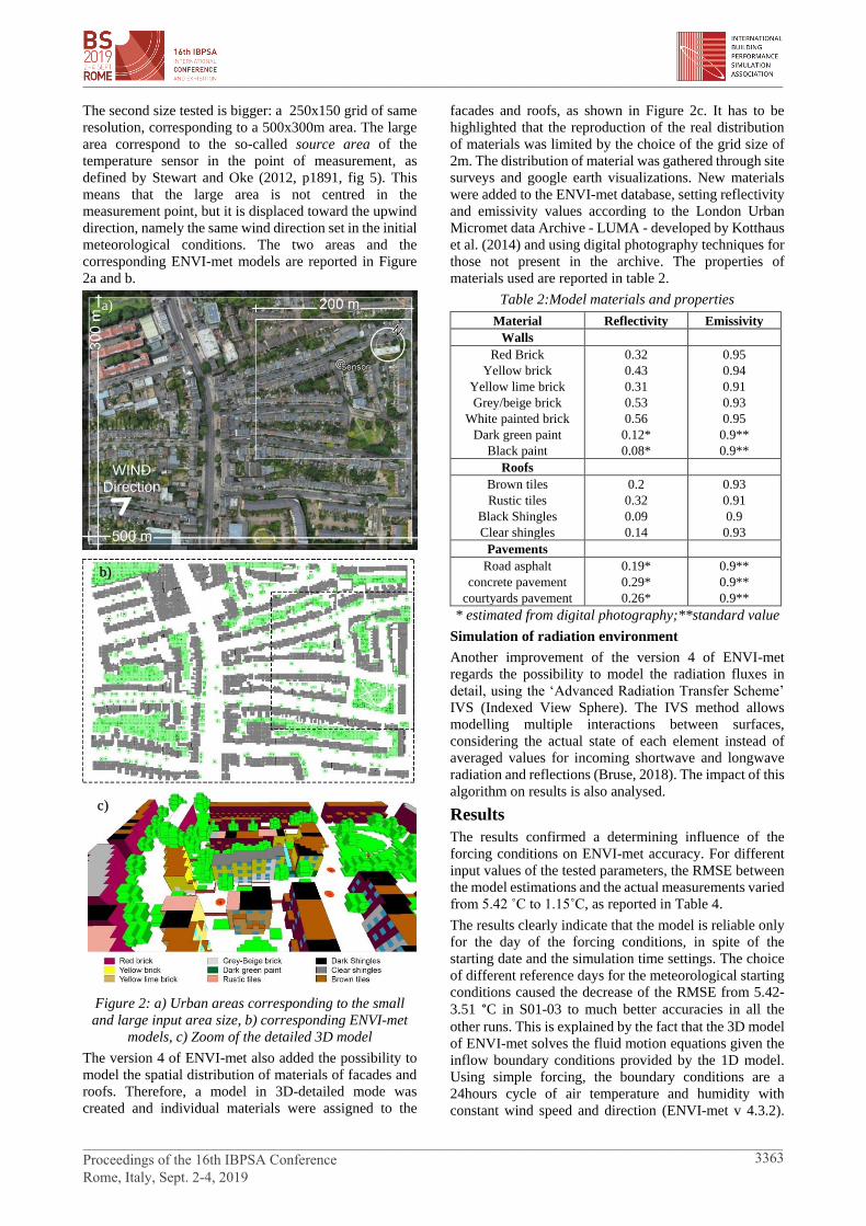
The second size tested is bigger: a 250x150 grid of same

resolution, corresponding to a 500x300m area. The large

area correspond to the so-called source area of the

temperature sensor in the point of measurement, as

defined by Stewart and Oke (2012, p1891, fig 5). This

means that the large area is not centred in the

measurement point, but it is displaced toward the upwind

direction, namely the same wind direction set in the initial

meteorological conditions. The two areas and the

corresponding ENVI-met models are reported in Figure

2a and b.

Figure 2: a) Urban areas corresponding to the small

and large input area size, b) corresponding ENVI-met

models, c) Zoom of the detailed 3D model

The version 4 of ENVI-met also added the possibility to

model the spatial distribution of materials of facades and

roofs. Therefore, a model in 3D-detailed mode was

created and individual materials were assigned to the

facades and roofs, as shown in Figure 2c. It has to be

highlighted that the reproduction of the real distribution

of materials was limited by the choice of the grid size of

2m. The distribution of material was gathered through site

surveys and google earth visualizations. New materials

were added to the ENVI-met database, setting reflectivity

and emissivity values according to the London Urban

Micromet data Archive - LUMA - developed by Kotthaus

et al. (2014) and using digital photography techniques for

those not present in the archive. The properties of

materials used are reported in table 2.

Table 2:Model materials and properties

Material Reflectivity Emissivity

Walls

Red Brick

Yellow brick

Yellow lime brick

Grey/beige brick

White painted brick

Dark green paint

Black paint

0.32

0.43

0.31

0.53

0.56

0.12*

0.08*

0.95

0.94

0.91

0.93

0.95

0.9**

0.9**

Roofs

Brown tiles

Rustic tiles

Black Shingles

Clear shingles

0.2

0.32

0.09

0.14

0.93

0.91

0.9

0.93

Pavements

Road asphalt

concrete pavement

courtyards pavement

0.19*

0.29*

0.26*

0.9**

0.9**

0.9**

* estimated from digital photography;**standard value

Simulation of radiation environment

Another improvement of the version 4 of ENVI-met

regards the possibility to model the radiation fluxes in

detail, using the ‘Advanced Radiation Transfer Scheme’

IVS (Indexed View Sphere). The IVS method allows

modelling multiple interactions between surfaces,

considering the actual state of each element instead of

averaged values for incoming shortwave and longwave

radiation and reflections (Bruse, 2018). The impact of this

algorithm on results is also analysed.

Results

The results confirmed a determining influence of the

forcing conditions on ENVI-met accuracy. For different

input values of the tested parameters, the RMSE between

the model estimations and the actual measurements varied

from 5.42 ˚C to 1.15˚C, as reported in Table 4.

The results clearly indicate that the model is reliable only

for the day of the forcing conditions, in spite of the

starting date and the simulation time settings. The choice

of different reference days for the meteorological starting

conditions caused the decrease of the RMSE from 5.42-

3.51 °C in S01-03 to much better accuracies in all the

other runs. This is explained by the fact that the 3D model

of ENVI-met solves the fluid motion equations given the

inflow boundary conditions provided by the 1D model.

Using simple forcing, the boundary conditions are a

24hours cycle of air temperature and humidity with

constant wind speed and direction (ENVI-met v 4.3.2).

WIND Direction

a)

b)

c)

________________________________________________________________________________________________


3363

For this reason, the results are reliable only for the day

used to set the forcing conditions. However, this issue has

been already overcome with the last releases of the

software such as the ENVI-met 4.4 Winter 1819 that

enabled full meteorological forcing including air

temperature and humidity, solar radiation, wind speed and

direction for longer meteorological periods.

Table 3: Parameters tested and relevant simulation ID

Variable Values/Method Sim ID

Sim starting

day

4th of August

5th of August

01-03

04-12

Air Temp

(°C)

22.0* (Heathrow)

23.8* (Measurements)

22.7* (UWG)

01

02-11

12

Wind speed

(m/s)

4.0 (Heathrow )

2.0 (K. & G. method)

1.4 (K. & G. method)

2.5 (BS 5925:1991)

-

01- 03

04

05-12

Buffer time

(hours)

48

24

06

01-05;07-12

Rad fluxes

(sim. method)

IVS On

IVS OFF

07

01-06;08-12

Area size

(m)

200x200x60

500x300x80

01-07;10-12

08-09

Materials of

wall and roof

Single material

Individual materials

01-02;08;10

03-07;09;11;12

* mean value of the hourly data used for simple forcing

Table 4: Accuracy of ENVI-met air temperature

estimations at 5m height

Sim ID RMSE MAE d R

squared

S_01 5.42 -5.19 0.74 0.95

S_02 4.38 -4.19 0.81 0.96

S_03 3.51 -3.20 0.86 0.96

S_04 1.45 -1.17 0.97 0.99

S_05 1.29 -0.86 0.98 0.99

S_06 1.41 -0.99 0.98 0.99

S_07 1.44 -1.11 0.97 0.99

S_08 1.41 -0.78 0.97 0.99

S_09 1.66 0.48 0.96 0.98

S_10 1.15 0.48 0.98 0.99

S_11 1.33 -0.42 0.98 0.97

The results also show that ENVI-met provides much more

reliable results when local air temperatures (S02) instead

of airport data (S10) are used to force the simulation.

When the meteorological input settings are well chosen,

the RMSE variability strongly decreases (S04-S12). Both

measured local air temperatures (S04-S11) and

estimations using urban energy balance models such as

UWG (S12) proved to be suitable input data.

As for the wind speed, the power law given by the BS

5925:1991 provides better accuracy than the coefficients

given by Kofoed & Gaardsted to estimate the wind speed

attenuation due to the urban roughness. However, using

the two methods, the RMSE change was minimal, from

1.45 °C in S04 to 1.29 °C in S05. Furthermore, wind speed

measurements would be necessary to validate this input

parameter.

The impact of the other input parameters on the air

temperature estimations is much less significant than the

meteorological settings. This is shown in Figure 3, which

represents just the results of the simulations forced with

local air temperature of the same day of comparison. The

RMSE variation determined by the size of the model and

the material distribution is between 1.45 °C and 1.15 °C.

Figure 3: Comparison of the modelled and measured

diurnal cycles of air temperature at 5m height of the

simulations forced with the meteorological conditions of

the same day of comparison, considering 24hrs buffer

time

The area size determines significant changes in the wind

field (speed and direction) which affect air temperature

estimations. According to this study, the results are more

accurate for small areas (about 200mx200m) than large

areas (300x500m). The simulation performed with the

large model, with detailed material specifications and

using local air temperatures as input, resulted in a

significant overestimation of the air temperature during

the night time (S09 in Figure 3). This probably happens

because of an overestimation of the urban effect. One

time, due to the significant reduction of the wind speed in

the big model compared to the small model. The second

time, due to the use of the local air temperatures as input,

which already embed the air temperature increase

determined by the characteristics of the urban fabric,

including the wind speed decrease (Salvati et al. 2016 &

2017, Kolokotroni et al. 2008).

The impact of the detailed distribution of the materials of

facades and roof varies depending on other input

parameters. The large model was simulated using the

same material for roof and walls (S08 - material

reflectivity 0.3) and with a detailed distribution of

materials (S09); in this case, the RMSE increased from

1.42 °C (S08) to 1.66 °C (S09), which can be explained

by a redundant computation of the urban effect, as

previously commented. Conversely, with small input

areas, the specification of materials increases the accuracy

16

18

20

22

24

26

28

30

Cel

siu

s d

eg (°C

)

Time

Air temperature at 5m height5th August 2007

S_07 S_05S_04 S_08S_09 S_11S_12 Measurements

________________________________________________________________________________________________


3364

of the estimation, but the impact varies depending on the

reflectivity chosen for the uniform material and the input

wind speed. For example, the specification of materials in

S03 (wind speed 2 m/s), determined a decrease of the

RMSE of almost 1 °C compared to S02. However, for

higher wind speed (2.5 m/s) and for albedo values of the

uniform material closer to the actual ones, the difference

in RMSE is much lower. In fact, the RMSE only varied

from 1.16 °C to 1.15 °C between S10 in S11, where S11

has the detail distribution of materials (Figure 2c and

Table 2) and S10 uniform materials for walls and roof, set

to clear shingles (r=0.14) and red brick (r=0.32).

However, the materials of facades and roofs do have an

impact on the distribution of surface temperatures.

Finally, the use of the IVS method did not improve the

accuracy of air temperature estimations. It had a

significant impact on the radiation balances within the

canyon, but at the cost of an extremely longer

computation time: the simulation with a super computer

lasted about 120 hours versus 38 hours without IVS.

Similarly, the consideration of a buffer time longer than

24 hours did not changed the results.

Among the set of simulations, the best accuracy was

achieved by S10, with a RMSE of 1.15 °C. This

corresponds to an input area of about 200x200m, with

detailed specification of facades and roofs materials,

using as forcing conditions the site temperature

measurements and the BS5925:1990 for wind speed

attenuation from airport data. It has to be highlighted that

all the simulations underestimated the air temperature

during daytime. The results of S_10 provided the best

approximation during daytime, but also a slight

overestimation of the nighttime temperature.

Microclimate variations across the calibrated model

The results also confirmed that the variations of the

climate variables across the 200x200m domain are

significant in terms of wind speed and mean radiant

temperature, while they are not in terms of air

temperature. The graphs in figure 5 show the diurnal cycle

of these variables at 5m height across the different

receptors placed in the model as represented in Figure 4.

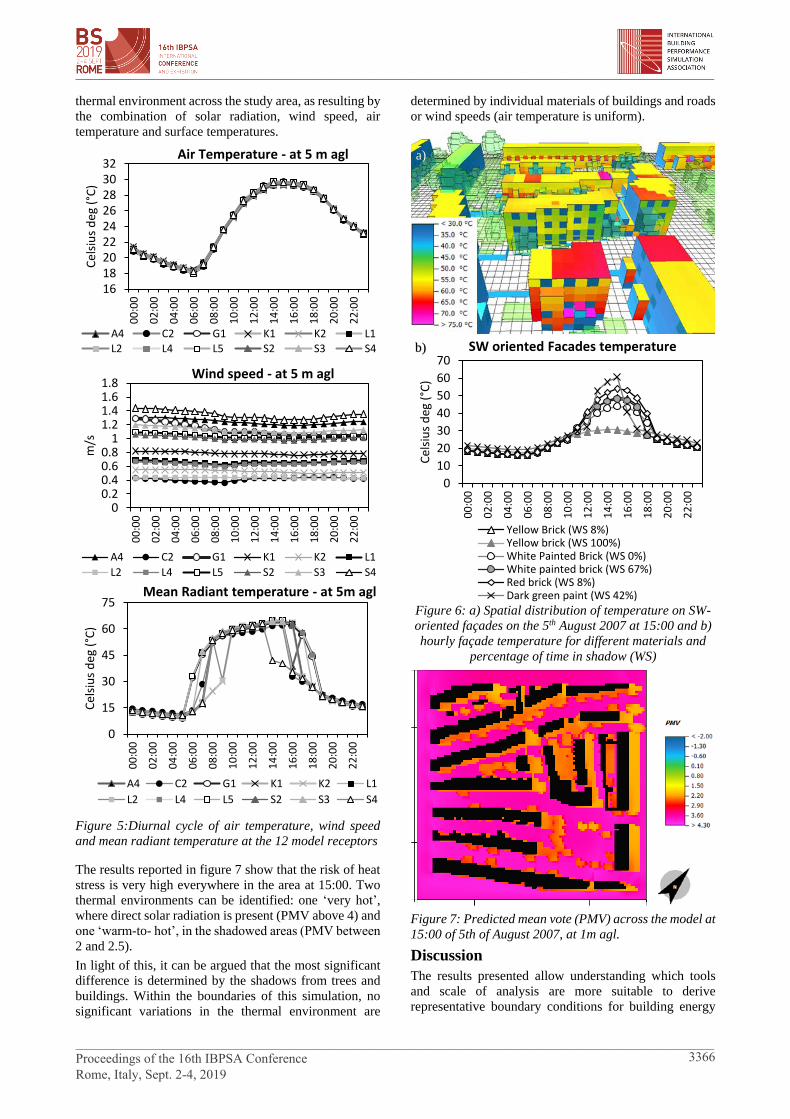
The first graph in Figure 5 shows that the air temperature

at 5m height is almost the same across the different

receptors of the model, throughout the day. The maximum

relative difference is around 0.55°C and occurs between

11:00 and 14:00, between the point L5 (hotter) and points

K1 and K2 (colder). This probably happens because the

surfaces around point L5 receive much more radiation

over the morning compared to K1 and K2, due to

geometry and orientation; L2 is not in an urban canyon as

opposite to K1 and K2 and it faces a south-east oriented

façade. However, the difference in terms of air

temperature is not significant. Closer to the ground level,

the diurnal air temperature differences are slightly higher:

at 1.8m agl, the maximum relative difference reached 0.73

°C at 14:00, between the points L5 and C2. Conversely,

wind speed variations are significant across the model,

with differences up to 1 m/s in very short distances, such

as between the points S4 and C2, where the maximum and

minimum speeds are estimated respectively.

Also the mean radiant temperature varies significantly

across the model. The maximum relative difference over

the day reached 30.9 °C at 16:00 and occurred between

point L2 (63.7 °C) and C2 (32.8 °C), the latter being

located under one tree.

As for the façade temperature, the maximum differences

were found on the south-west oriented facades, due to the

higher impact of solar radiation. The temperature

difference on the south-west facades reached up to 30°C

at 15:00, between the irradiated portion painted in dark

green and the shadowed portion in bricks. However, the

temperature difference between the same two points

dramatically decreased to about 2 °C at 19:00, due to the

beneficial effect of shadows on the dark green surface.

Figure 4: Location of the 12 receptors in the model, where

point A4 corresponds to the location of the site

temperature sensor

Both the surface temperatures and the mean radiant

temperatures are driven by the amount of direct solar

radiation received by the surfaces and, therefore, by the

surrounding urban geometry and facades orientation.

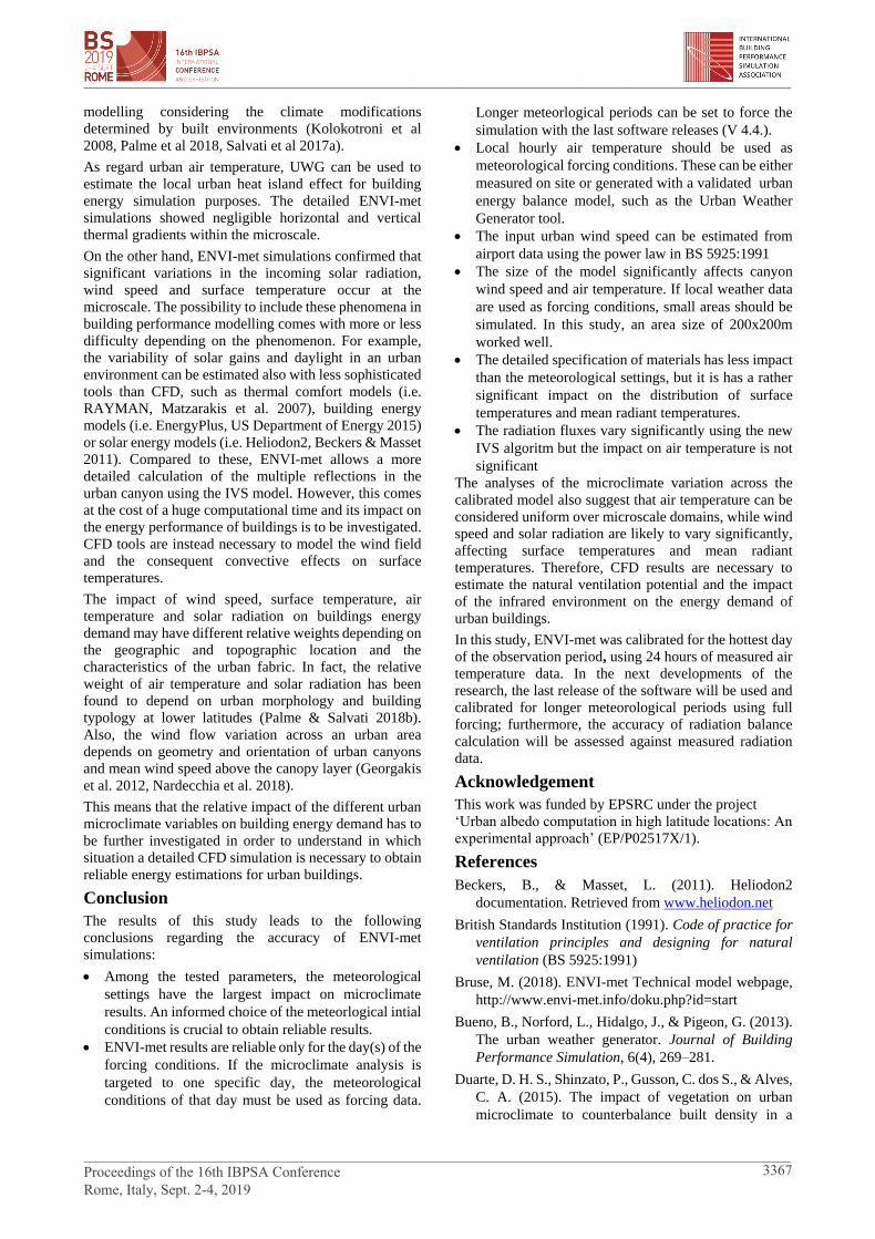
This is clear also from the results for the Predicted Mean

Vote (PMV) reported in Figure 7. The PMV is a thermal

index developed by Fanger (1982) to assess indoor

thermal comfort. The PMV calculated by ENVI-met has

been adapted for outdoor conditions, including solar

radiation and wind speed. In an indoor environment, the

PMV normally varies between -4 and +4, where zero

means thermally neutral, -4 means very cold and +4 very

hot. The PMV was developed based on experiments on

indoor environments and its use for outdoors is not fully

reliable. Furthermore, it has been known that the

physiological approach alone is not sufficient to

characterise human thermal comfort in outdoor

environments (Nikolopoulou, 2001). Therefore, the PMV

is used in this study just to highlight the variability of the

________________________________________________________________________________________________


3365

thermal environment across the study area, as resulting by

the combination of solar radiation, wind speed, air

temperature and surface temperatures.

Figure 5:Diurnal cycle of air temperature, wind speed

and mean radiant temperature at the 12 model receptors

The results reported in figure 7 show that the risk of heat

stress is very high everywhere in the area at 15:00. Two

thermal environments can be identified: one ‘very hot’,

where direct solar radiation is present (PMV above 4) and

one ‘warm-to- hot’, in the shadowed areas (PMV between

2 and 2.5).

In light of this, it can be argued that the most significant

difference is determined by the shadows from trees and

buildings. Within the boundaries of this simulation, no

significant variations in the thermal environment are

determined by individual materials of buildings and roads

or wind speeds (air temperature is uniform).

Figure 6: a) Spatial distribution of temperature on SW-

oriented façades on the 5th August 2007 at 15:00 and b)

hourly façade temperature for different materials and

percentage of time in shadow (WS)

Figure 7: Predicted mean vote (PMV) across the model at

15:00 of 5th of August 2007, at 1m agl.

Discussion

The results presented allow understanding which tools

and scale of analysis are more suitable to derive

representative boundary conditions for building energy

161820222426283032

00

:00

02

:00

04

:00

06

:00

08

:00

10

:00

12

:00

14

:00

16

:00

18

:00

20

:00

22

:00

Cel

siu

s d

eg (°C

)

Air Temperature - at 5 m agl

A4 C2 G1 K1 K2 L1L2 L4 L5 S2 S3 S4

00.20.40.60.8

11.21.41.61.8

00

:00

02

:00

04

:00

06

:00

08

:00

10

:00

12

:00

14

:00

16

:00

18

:00

20

:00

22

:00

m/s

Wind speed - at 5 m agl

A4 C2 G1 K1 K2 L1

L2 L4 L5 S2 S3 S4

0

15

30

45

60

75

00

:00

02

:00

04

:00

06

:00

08

:00

10

:00

12

:00

14

:00

16

:00

18

:00

20

:00

22

:00

Cel

siu

s d

eg (°C

)

Mean Radiant temperature - at 5m agl

A4 C2 G1 K1 K2 L1

L2 L4 L5 S2 S3 S4

0

10

20

30

40

50

60

70

00

:00

02

:00

04

:00

06

:00

08

:00

10

:00

12

:00

14

:00

16

:00

18

:00

20

:00

22

:00

Cel

siu

s d

eg (

°C)

SW oriented Facades temperature

Yellow Brick (WS 8%)Yellow brick (WS 100%)White Painted Brick (WS 0%)White painted brick (WS 67%)Red brick (WS 8%)Dark green paint (WS 42%)

a)

b)

________________________________________________________________________________________________


3366

modelling considering the climate modifications

determined by built environments (Kolokotroni et al

2008, Palme et al 2018, Salvati et al 2017a).

As regard urban air temperature, UWG can be used to

estimate the local urban heat island effect for building

energy simulation purposes. The detailed ENVI-met

simulations showed negligible horizontal and vertical

thermal gradients within the microscale.

On the other hand, ENVI-met simulations confirmed that

significant variations in the incoming solar radiation,

wind speed and surface temperature occur at the

microscale. The possibility to include these phenomena in

building performance modelling comes with more or less

difficulty depending on the phenomenon. For example,

the variability of solar gains and daylight in an urban

environment can be estimated also with less sophisticated

tools than CFD, such as thermal comfort models (i.e.

RAYMAN, Matzarakis et al. 2007), building energy

models (i.e. EnergyPlus, US Department of Energy 2015)

or solar energy models (i.e. Heliodon2, Beckers & Masset

2011). Compared to these, ENVI-met allows a more

detailed calculation of the multiple reflections in the

urban canyon using the IVS model. However, this comes

at the cost of a huge computational time and its impact on

the energy performance of buildings is to be investigated.

CFD tools are instead necessary to model the wind field

and the consequent convective effects on surface

temperatures.

The impact of wind speed, surface temperature, air

temperature and solar radiation on buildings energy

demand may have different relative weights depending on

the geographic and topographic location and the

characteristics of the urban fabric. In fact, the relative

weight of air temperature and solar radiation has been

found to depend on urban morphology and building

typology at lower latitudes (Palme & Salvati 2018b).

Also, the wind flow variation across an urban area

depends on geometry and orientation of urban canyons

and mean wind speed above the canopy layer (Georgakis

et al. 2012, Nardecchia et al. 2018).

This means that the relative impact of the different urban

microclimate variables on building energy demand has to

be further investigated in order to understand in which

situation a detailed CFD simulation is necessary to obtain

reliable energy estimations for urban buildings.

Conclusion

The results of this study leads to the following

conclusions regarding the accuracy of ENVI-met

simulations:

Among the tested parameters, the meteorological

settings have the largest impact on microclimate

results. An informed choice of the meteorlogical intial

conditions is crucial to obtain reliable results.

ENVI-met results are reliable only for the day(s) of the

forcing conditions. If the microclimate analysis is

targeted to one specific day, the meteorological

conditions of that day must be used as forcing data.

Longer meteorlogical periods can be set to force the

simulation with the last software releases (V 4.4.).

Local hourly air temperature should be used as

meteorological forcing conditions. These can be either

measured on site or generated with a validated urban

energy balance model, such as the Urban Weather

Generator tool.

The input urban wind speed can be estimated from

airport data using the power law in BS 5925:1991

The size of the model significantly affects canyon

wind speed and air temperature. If local weather data

are used as forcing conditions, small areas should be

simulated. In this study, an area size of 200x200m

worked well.

The detailed specification of materials has less impact

than the meteorological settings, but it is has a rather

significant impact on the distribution of surface

temperatures and mean radiant temperatures.

The radiation fluxes vary significantly using the new

IVS algoritm but the impact on air temperature is not

significant

The analyses of the microclimate variation across the

calibrated model also suggest that air temperature can be

considered uniform over microscale domains, while wind

speed and solar radiation are likely to vary significantly,

affecting surface temperatures and mean radiant

temperatures. Therefore, CFD results are necessary to

estimate the natural ventilation potential and the impact

of the infrared environment on the energy demand of

urban buildings.

In this study, ENVI-met was calibrated for the hottest day

of the observation period, using 24 hours of measured air

temperature data. In the next developments of the

research, the last release of the software will be used and

calibrated for longer meteorological periods using full

forcing; furthermore, the accuracy of radiation balance

calculation will be assessed against measured radiation

data.

Acknowledgement

This work was funded by EPSRC under the project

‘Urban albedo computation in high latitude locations: An

experimental approach’ (EP/P02517X/1).

References

Beckers, B., & Masset, L. (2011). Heliodon2

documentation. Retrieved from www.heliodon.net

British Standards Institution (1991). Code of practice for

ventilation principles and designing for natural

ventilation (BS 5925:1991)

Bruse, M. (2018). ENVI-met Technical model webpage,

http://www.envi-met.info/doku.php?id=start

Bueno, B., Norford, L., Hidalgo, J., & Pigeon, G. (2013).

The urban weather generator. Journal of Building

Performance Simulation, 6(4), 269–281.

Duarte, D. H. S., Shinzato, P., Gusson, C. dos S., & Alves,

C. A. (2015). The impact of vegetation on urban

microclimate to counterbalance built density in a

________________________________________________________________________________________________


3367

http://www.heliodon.net/

subtropical changing climate. Urban Climate, 14,

224–239.

Fanger, P. O. (1982). Thermal Comfort. Analysis and

Application in Environment Engineering. McGraw

Hill Book Company, New York.

Georgakis, C., & Santamouris, M. (2012). Wind and

Temperature in the Urban Environment. In F. Allard

& C. Ghiaus (Eds.), Natural Ventilation in the Urban

Environment: Assessment and Design. Routledge.

London (UK).

Goldber, V., Kurbjuhn, C., & Bernhofer, C. (2013). How

relevant is urban planning for the thermal comfort of

pedestrians? Numerical case studies in two districts of

the City of Dresden (Saxony/Germany).

Meteorologische Zeitschrift, 22(6), 739–751.

Kofoed, N.-U., & Gaardsted, M. (2004). Considerations

of the Wind in Urban Spaces. In M. Nikolopoulou

(Ed.), Designing open spaces in the urban

environment: a bioclimatic approach rediscovering

the urban realm and open spaces, key action 4 “City

of tomorrow and cultural Heritage” from the

programme “Energy, Environment and Sustainable

Development”. Centre for Renewable Energy Sources

(C.R.E.S.), Greece

Kolokotroni, M., & Giridharan, R. (2008). Urban heat

island intensity in London: An investigation of the

impact of physical characteristics on changes in

outdoor air temperature during summer. Solar Energy

82(11), 986–998.

Kolokotroni, M., Giannitsaris, I., & Watkins, R. (2006).

The effect of the London urban heat island on building

summer cooling demand and night ventilation

strategies. Solar Energy, 80(4), 383–392.

Kotthaus, S., Smith, T. E. L., Wooster, M. J., &

Grimmond, C. S. B. (2014). Derivation of an urban

materials spectral library through emittance and

reflectance spectroscopy. ISPRS Journal of

Photogrammetry and Remote Sensing, 94, 194–212.

Lindberg, F., Grimmond, C. S. B., Gabey, A., Huang, B.,

Kent, C. W., Sun, T., … Zhang, Z. (2018). Urban

Multi-scale Environmental Predictor (UMEP): An

integrated tool for city-based climate services.

Environmental Modelling and Software, 99, 70–87.

Mao, J. (2018). Automatic calibration of an urban

microclimate model under uncertainty. MSc thesis,

Massachusetts Institute of Technology.

Matzarakis, Andreas, Frank Rutz, and Helmut Mayer.

2007. “Modelling Radiation Fluxes in Simple and

Complex Environments--Application of the RayMan

Model.” International Journal of Biometeorology 51

(4): 323–34.

Nardecchia, F., Bernardino, A. Di, Pagliaro, F., Monti, P.,

Leuzzi, G., & Gugliermetti, L. (2018). CFD Analysis

of Urban Canopy Flows Employing the V2F Model :

Impact of Different Aspect Ratios and Relative

Heights. Advances in Meteorology, 2018, Article ID

2189234.

Nikolopoulou, M., Baker, N., & Steemers, K. (2001).

Thermal comfort in outdoor urban spaces:

Understanding the Human parameter. Solar Energy,

70(3), 227–235.

Oke, T. R., Mills, G., Christen, A., & Voogt, J. A. (2017).

Urban Climates. Cambridge University Press.

Cambridge (UK)

Palme, M., Inostroza, L., & Salvati, A. (2018a).

Technomass and cooling demand in South America: a

superlinear relationship? Building Research &

Information 46, 864–880.

Palme, M., & Salvati, A. (2018b). UWG -TRNSYS

Simulation Coupling for Urban Building Energy

Modelling. In Proceedings of BSO 2018: 4th Building

Simulation and Optimization Conference, Cambridge,

UK: 11-12 September 2018 (pp. 635–641).

Salata, F., Golasi, I., de Lieto Vollaro, R., & de Lieto

Vollaro, A. (2016). Urban microclimate and outdoor

thermal comfort. A proper procedure to fit ENVI-met

simulation outputs to experimental data. Sustainable

Cities and Society 26, 318–343.

Salvati, A., Coch, H., & Cecere, C. (2016). Urban Heat

Island Prediction in the Mediterranean Context: an

evaluation of the urban weather generator model.

ACE: Architecture, City and Environment =

Arquitectura, Ciudad Y Entorno, 11(32), 135–156.

Salvati, A., Coch, H., & Cecere, C. (2017a). Assessing the

urban heat island and its energy impact on residential

buildings in Mediterranean climate: Barcelona case

study. Energy and Buildings, 146, 38–54.

http://doi.org/10.1016/j.enbuild.2017.04.025

Salvati, A., Palme, M., & Inostroza, L. (2017b). Key

Parameters for Urban Heat Island Assessment in A

Mediterranean Context: A Sensitivity Analysis Using

the Urban Weather Generator Model. IOP Conference

Series: Materials Science and Engineering 245,

82055.

Stewart, I. D., & Oke, T. R. (2012). Local Climate Zones

for Urban Temperature Studies. Bulletin of the

American Meteorological Society 93(12), 1879–1900.

US Department of Energy. (2015). Engineering reference

The Reference to EnergyPlus Calculations.

________________________________________________________________________________________________


3368

microclimate data for building energy modelling: study on

Documents