Micro-Raman Manual

Masami Kanzaki mkanzaki@okayama-u.ac.jp (or mkanzaki@me.com)

Institute for Planetary Materials, Okayama U., Misasa, Japan revised Aug. 12, 2017

Our Micro-Raman spectrometer consists of a solid state laser (488 nm), micro-sam-pling system (back scattering geometry), Raman filters, an imaging monochromator (f=500 mm ), and LN2-cooled CCD detector (see Fig. 1). Please contact Dr. Masami Kanzaki for use (3rd building 3rd floor or mail). Join-use or cooperative research use are also possi-ble. Most of this work is supported by grants from JSPS and MEXT.

Outline of the instrument 488 nm laser: Coherent Sapphire longitudinal single mode. Output 100 mW, diameter ~ 0.7 mm. 785nm NIR laser and 532nm laser are also available. micro-sampling system: back scattering geometry, Mitsutoyo's long working distance (34 mm for x2-x10, 20 mm for x20, x50, and 13 mm for x100) objective lenses for DAC and heating stage. We also have ordinary working distance (but higher NA) objective lenses (x5, x10, x20, x50, x100) for ordinary samples and recovered run charges (also for thin DACs). Depolarizer is placed before the entrance slit. Raman filters: Semrock's Raman edge filters for 488, 514, 532, 632 and 785 nm. No anti-Stokes side observable with these filters. ONDAC SureBlock filters (only for 488 nm) are also available for low-frequency and anti-Stokes side. Dichroic beam splitters: Semrock's filter for 488, 514, 532, 632 and 785 nm. Laser line filters: 488, 514, 532 and 785 nm available Monochromator: Acton's SpectraPro 500i. F=5.6, f=500 mm monochromator/ spectrograph, Three gratings are available (300 g/mm, 1200 g/mm, 1800 g/mm). LN2-cooled CCD detector: Princeton Instruments' PyLoN 400BRX CCD detector, 1340x400 pix-el, back illuminated, eXcelon. Software: WinSpec (Roper) running under Windows 7 Pro (32 bit) for spectrum measurement. Lab-brewed softwares for Raman hardware control and ruby pressure scale are available.

1

Figure 1. Micro-Raman optical system (SureBlock-based configuration)

Figure 2. Difference between Semrock-based and Ondax-based optical configuration

2

Requests for users• Please contact Kanzaki for first-time use. • In order to avoid the dust, keep the doors closed (except LN2 filling time). • Take off dusts in your shoes by walking on the sticky mat at the entrance. • After the use, clean the tables. Put optical components back to the dry boxes.•When using the laser, keep laser power 70~100%. When not in use for a while, turn to Standby

mode (turn key switch anti-clockwise).•Record the conditions of the use on the lab notebook provided (laser power, measurement condi-

tions, time, etc), also on your lab notebook. Please report any troubles, incidents, and shortage of disposals to Kanzaki.

•When publishing a paper containing data from this spectrometer, please acknowledge. In order to fix and repair this spectrometer, we need such evidences to request from Institutional budgets (so far this instrument is mostly supported by my funds). A list of papers published using this spectrometer is given in later part.

How to use the instrument

Cool the CCD detector In order to use the instrument, you need to first cool CCD detector by liquid nitrogen (LN2).

1) Turn on air ventilation next to air-conditioning on the wall (usually ON). For further air ventila-tion, open the door. There is an oxygen monitor (Photo 1) on the anti-vibrational table. Make sure the oxygen monitor is working properly. When a lot of LN2 is spilled out or alarm of the oxygen monitor beeps, exit from the room immediately.

2) Make sure the CCD controller (Photo 2) is ON before refilling LN2. If you refill LN2 without turning it ON, you need to wait the CCD detector becomes room temperature again, wasting both your time and LN2. It is usually ON, but for long holidays etc, it will be turned off.

3) Draw LN2 from the LN2 tower outside of the main building to 10-liter dewar (Photo 3). Bring eye-protection glasses and cryogenic groves (Photo 4) with you, and put it during drawing. The number for a padlock for the tower is written on the dewar. Write date and how much drawn (litter) on a logbook stored at there, in the column of Kanzaki.

4) Make sure there is no water on a funnel (Photo 5) and a small dewar (Photo 4). Remove a lid from the CCD detector, and put the funnel in the CCD dewar (as shown in Photo 5). Use a black cube to support the funnel. Put on eye-protection glasses and leather gloves. Draw LN2 from the 10-liter dewar to small dewar (in Photo 4), then transfer to the CCD dewar using the funnel. There will be extensive evaporation when drawing LN2 first time. Pouring 2 times is enough for 8~10 hours use.

5) Remove the funnel. Put the lid back after the initial intense evaporation is over. 6) You can monitor current CCD temperature from WinSpec’s Setup menu, and check “Detector

Temperature”. Currently temperature is set to -120 ˚C, and kept by using a heater inside.7) If the temperature does not reach to -120 ˚C after more than 1 hour after pouring, please let Kan-

zaki know. Most likely vacuum state of the dewar becomes bad.

　　　

Photo 1. Oxygen monitor and laser protection glasses (for 488 nm)

3

Photo 2. Power unit for CCD controller. Make sure this power switch is ON before filling LN2

Photo 3. 10-L liquid nitrogen dewar

Photo 4. Right: Cryo-glove and protection glasses; Left: small de-war

Photo 5. Funnel for LN2 and black cube placed on top of the CCD dewar

　　　　　　　　　　　　　　　　

4

How to operate the 488 nm 100mW laser (Class 3B)

Wear laser-protection glasses (Photo 1) whenever laser is in operation. Do not see direct laser beams and reflected beams by naked eyes. 1) Turn ON power switch on the back side of the 488 nm laser controller (Photo 6). Wait until

“Standby” appears in the display. Then turn the key switch clock-wise.

2) In order to change power(%), turn the nob. This will change setting for power (upper). 100% means 100 mW. Push the nob momentary to change the power (in short time, laser output be-comes 0%, and comes back to set power). Based on the manual, 70~100% power is recommend-ed, so please use laser power% in this range.

Photo 6. Front panel of Coherent Sapphire 488 nm laser controller

Photo 7. Window of Raman-controller program (Raman2). When started, select COM4 as the serial port. This program will control IN/OUT of beam splitters (BS1,2), ON/OFF of il-lumination lights, ON/OFF of ND filter for the laser.

Photo 8. Standard samples (synthetic coesite and natural diamond) for optical adjustments and cali-brations

Photo 9. Black control box. Only two variable

resisters are active to change brightness of il-lumination lights

5

How to operate the 532 nm laser (Class 3B) (optional) Wear laser-protection glasses for 532 nm . This laser will be used when the 488 nm laser is not available or to avoid fluorescence. Please ask Kanzaki for replacement, optical alignment etc. 1) Turn ON the power switch on the front side of the 532 nm laser controller (Photo 10). Wait 4

minutes, and then turn the key switch clock-wise. When not in use for a while, turn the key switch counter-clockwise.

2) No way to change power (always 100 mW output).

3) In past, long-time continuous use (few hours) caused laser output down, or mode-hopping. So use with care.

For the 785 nm solid laser, please ask Dr. Kanzaki. To use it, replacements of optics and alignments of mirrors (as well as change of protection glasses) are necessary.

Photo 10. Front panel of 532 nm (G4+) laser controller

Photo 11. Power switch for Raman-control hardware

6

Measurement of Raman spectra 1) Ware laser protection glasses. Turn ON power switch (Photo 11) on the anti-vibration table. ND

filter, BS splitters for CCD camera and reflection light, switches for fiber light sources are all controlled through PC. Turn on the PC.

2) Turn ON the laser (see the instruction above). Double click WinSpec icon on the desktop of the PC. It will take a while to see opening graphics of WinSpec. From the Acquisition menu, select “Experimental Setup …”. In Data File tab, check “Use a new window for each run”, and click OK button. You also need “Info” window to check cursor positions (and relative wave number), and it can be opened by selecting Info from View menu.

3) Double click the Raman2 icon on the desktop. Photo 7 shows appearance of this application. This application can control two beam splitters (BS1, BS2), illumination (reflection and trans-mission) lights, and ND filter for the laser. The ND filter is rotational type, and density gradually change with angle, and its rotational angle is controlled by a servo motor. At OFF position, most laser beam is absorbed, and at ON position, laser is not absorbed. Please note that even OFF po-sition, some laser light is still coming to sample side, which allows us to locate the laser spot on the sample image.

4) Place single crystal diamond (or anything else which emits strong Raman peaks) on the stage. You can use my standard sample (single crystal diamond originally used for DAC) (Photo 8). Turn on reflection illuminator from the “Raman controller” by clicking “Ref. light” button (or “Trans light”, if sample is thin and transparent). You will see a weak laser spot when illumina-tion light is dim. Find proper place of the sample, and move it to the laser spot by XYZ stage. Illumination light’s intensity can be adjusted by a variable resistor of the black box on the table (Photo 9). Please note that in order to observe the image, BS2 should be IN, as this BS2 is used to bring image to a camera. Also BS1 is reflecting illumination light to the sample, so it should be IN, when using the reflection light illumination.

5) When the position and focus are adjusted, you are ready to measure Raman spectrum. Click “BS1” and “BS2” button in Raman-control (Photo 7) to OUT these beam splitters. Then turn off illumination light(s) by clicking “Ref. Light” or “Trans. Light” button. Finally click “Laser” but-ton to introduce laser light to the sample. (Currently “Measure” button has problem, and do not use). For these buttons, shown (ON or OFF) are current state.

6) Select Exp. Setup from Acquisition menu of WinSpec. On Main tab, set the measuring time to 1s and use focus mode to observe spectrum continuously (Figure 3). This focus mode will mea-sure and display spectrum every selected time interval, so it is suited for alignment and quick test measurement. Generally a grating of 1200 g/mm is selected and center wave number will be 800 or 900 cm -1. If not, select 1200 g/mm grating and rotate it to 800 or 900 cm-1 using Move... of Spectrograph's menu. In the case of diamond, there will be single peak at 1332 cm-1. If wavenumber is different more than few cm-1, you should do wavenumber calibration first (see “Adjustment”section). Very sharp and strong peaks appear in a scan, but disappear in a next scan, are due to cosmic rays. Once 1332 cm-1 peak is found, adjust focus by looking the intensity of the peak. It is easy to see the change of intensity by fixing the intensity scale. This can be done by selecting Layout from Display menu, and fix the range of the intensity by unchecking a box (default is autoscale). In the case of diamond with 50 micron slit width, 100 mW laser power, binning=400, 200 micron pinhole, one second exposure, the intensity of 1332 cm-1 would be higher than 64,000 counts (means saturated). If count is very low, current alignment has prob-lem. See “Adjustment” section or ask Kanzaki for re-alignment.

7

7) If alignment is OK, replace diamond with your sample, and move a point of interest of your sample to the laser spot. Then adjust laser power to adequate level, and set appropriate exposure time and so on in Exp. Setup window, and then start measurement by clicking Acquire button (Fig. 3).

8) You can improve your spectrum by changing laser power (if not 100%), longer exposure time and accumulation numbers. Please note that spectrum taken for 1s exposure for 60 times, and that for 60s exposure for 1 time are different (check by yourself). Latter is better (due to reading noise). So it is better to use longer exposure time. However, peak intensity may saturate (>64,000 count) for some cases. For that case, reduce exposure time, and increase accumulation number, as accumulation is done on PC, no saturation happens. Once good spectra are obtained. Save the spectra from Edit menu.

9) If measurement is finished, write down the conditions of the measurements for record. The spec-trum data files are special binary format, and can not be read by ordinary programs (Excel etc). Convert them to ascii text files using “Ascii Conversion” from Tools' menu. Example of typical spectrum for synthetic coesite plotting from text data file is shown in Figure 4.

Figure 3. Experimental setup window (Main tab)

Figure 4. Raman spectrum of synthetic coesite (with SureBlock filters) 8

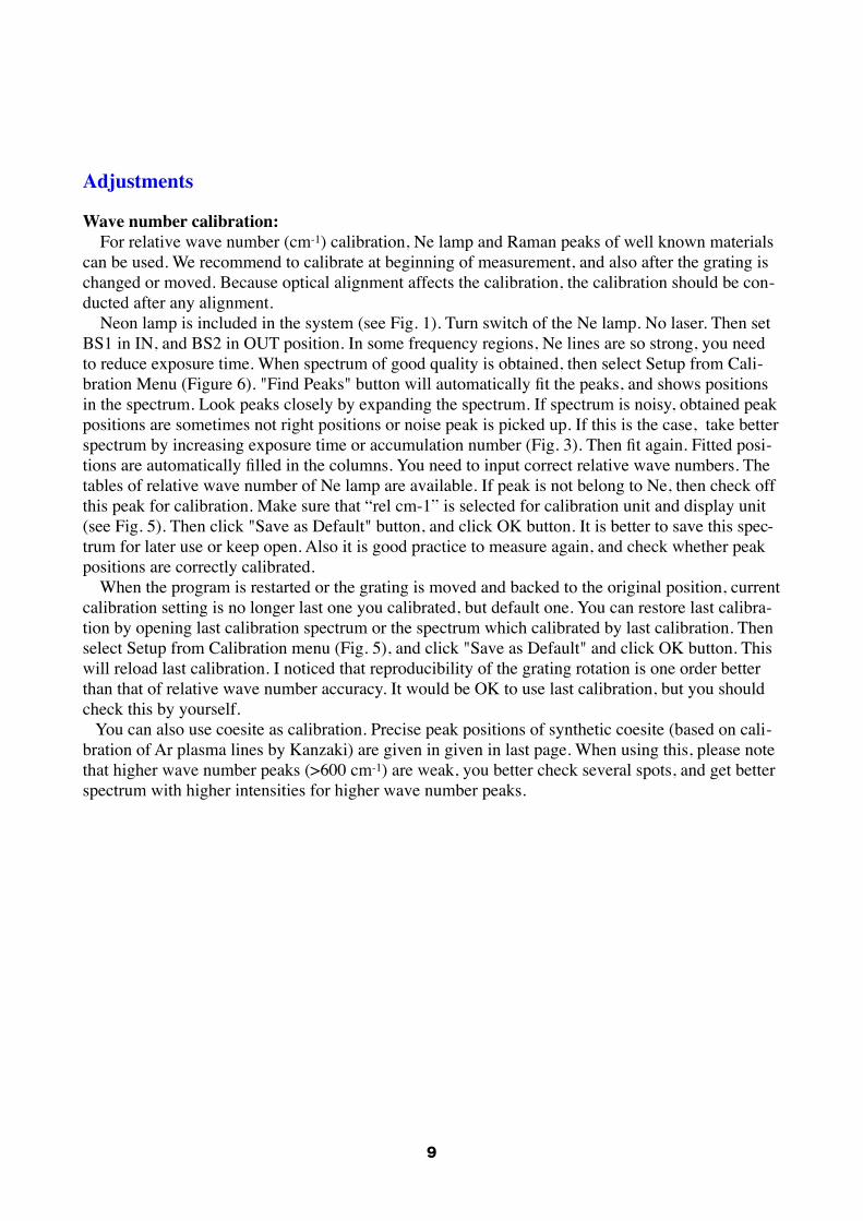
Adjustments

Wave number calibration: For relative wave number (cm-1) calibration, Ne lamp and Raman peaks of well known materials can be used. We recommend to calibrate at beginning of measurement, and also after the grating is changed or moved. Because optical alignment affects the calibration, the calibration should be con-ducted after any alignment. Neon lamp is included in the system (see Fig. 1). Turn switch of the Ne lamp. No laser. Then set BS1 in IN, and BS2 in OUT position. In some frequency regions, Ne lines are so strong, you need to reduce exposure time. When spectrum of good quality is obtained, then select Setup from Cali-bration Menu (Figure 6). "Find Peaks" button will automatically fit the peaks, and shows positions in the spectrum. Look peaks closely by expanding the spectrum. If spectrum is noisy, obtained peak positions are sometimes not right positions or noise peak is picked up. If this is the case, take better spectrum by increasing exposure time or accumulation number (Fig. 3). Then fit again. Fitted posi-tions are automatically filled in the columns. You need to input correct relative wave numbers. The tables of relative wave number of Ne lamp are available. If peak is not belong to Ne, then check off this peak for calibration. Make sure that “rel cm-1” is selected for calibration unit and display unit (see Fig. 5). Then click "Save as Default" button, and click OK button. It is better to save this spec-trum for later use or keep open. Also it is good practice to measure again, and check whether peak positions are correctly calibrated. When the program is restarted or the grating is moved and backed to the original position, current calibration setting is no longer last one you calibrated, but default one. You can restore last calibra-tion by opening last calibration spectrum or the spectrum which calibrated by last calibration. Then select Setup from Calibration menu (Fig. 5), and click "Save as Default" and click OK button. This will reload last calibration. I noticed that reproducibility of the grating rotation is one order better than that of relative wave number accuracy. It would be OK to use last calibration, but you should check this by yourself. You can also use coesite as calibration. Precise peak positions of synthetic coesite (based on cali-bration of Ar plasma lines by Kanzaki) are given in given in last page. When using this, please note that higher wave number peaks (>600 cm-1) are weak, you better check several spots, and get better spectrum with higher intensities for higher wave number peaks.

9

�

Figure 5. Window of calibration setup

Optical alignments: If not used a while, when optics are changed, and after earthquakes, alignments of the system are changed, and obtained intensity will be lower compared to previous runs. In this case, the align-ments of some optics are necessary. There are two places the user can adjust. One is the lens before the entrance slit of the mono-chromator. If you can not observed any diamond peak, then first remove the pinhole (for confocal configuration). Then widen the entrance slit. Then adjust position of the lens. After this, put the pin-hole back, and adjust the pinhole position. This may take a while. If you failed to get good result, ask Kanzaki for the alignment.

Selection and rotation of gratings: This monochromator hosts three gratings, and you can select one for your own purpose. A 300/mm grating is good for take a spectrum of wider range of frequency at once. It may useful to see distribution of fluorescence light. A 1200/mm grating is for general purpose and is our default, and is commonly used to take fundamental modes of most materials at once. If more accuracy is need-ed, you can choose a 1800/mm grating. If you want to observe other frequency or wave number region, you need to rotate the grating. These grating and it's center frequency at center of spectrum, can be selected from Move... of Spectrograph's menu (Fig. 6). Select grating and central frequency, and click OK button. When grating passes the laser line frequency, alert box will pop-up. Just click OK. For standard measurement, move to 800~900 cm-1. When using SureBlock filters, move to lower wave number to see not only Stokes side, but anti-Stokes side. In order to observe OH stretching region, move to ~3300 cm-1, but for strong hydrogen bonding case, you will need to measure lower wave number too. For ruby pressure scale (using 488 nm laser), move to ~6200 cm-1 which is close to R1 peak position of ruby. At this region, several strong Ne lines can be observed (see table of page 11).

10

�Figure 6. Move spectrograph window

Change of slit size: A width of an entrance slit of the monochromator can be changed manually. For change, rotate the micrometer head placed at the entrance slit. One turn corresponds to 250 micron. It is recom-mended to set the width smaller than 100 micron, as peak shape and width are not good. My default is 50 micron.

Change of binning: Software default is All (=400 pixels). But you can select smaller number to avoid noises from outside of laser spot, as generally only central 10-20 pixels will receive actual Raman scatterings. For change, select EasyBinning from Exp. Setup menu. Use focus to continuously get the spectrum. Then from Display, change the spectrum to “image”. Then you can see the image, not spectrum. You will see Raman scattering spots falling in the central horizontal zone of CCD. It they deviate from the center, you can adjust it by moving the lens (Z-direction) in front of the entrance slit. Then change the binning to 10 to 20, and press OK button on the EasyBinning window. From next mea-surement, new binning will be used.

Change to SureBlock or back: This will be challenging for ordinary user. Ask Kanzaki for change.

　

Advanced measurements Spectrum processing You can do spectrum processing using WinSpec, but it is generally not very good. So you need to process data using other softwares. A fitting software called fityk (www.unipress.waw.pl/fityk), developed by Institute of High Pressure Physics, Polish Academy of Sciences, can read SPE file which is native format of WinSpec. Background removal and fitting peaks by Gaussian, Lorentzian and other functions are possible. It runs on Windows, Mac OS X and Linux. CrystalSleuth, a program developed by Prof. Bob Downs’s group at University of Arizona, is installed in the PC. You can plot spectrum (after conversion of original file to a text file in WinSpec), and comic-ray removal, and background subtraction are possible. Also the program can search RRUFF mineral Raman database to identify phase(s) using your Raman spectrum.

Measurements using DAC and heating stage We provide long-working distance objective lenses for DAC and heating stage. Also sample stage can be modi-fied to accommodate most of devices we have. So far, several DACs and heating stages (home-build heating wire device) are used with this spectrometer without problem.

Ruby fluorescence (pressure scale) measurement

11

If you are doing DAC study, you will need to measure ruby R1 first at ambient pressure, then Raman measure-ment at different wave length region, and again come back to R1, and so on. In this case, it is convenient to do all measurements using relative wave number, without changing unit of horizontal axis. For this purpose, tables of neon lines for calibration using relative wave numbers are given below.

Using this relative wave numbers given in the tables, we can calibrate the X scale. Using this cal-ibration, determine relative wave number of ruby R1 peak. If you are not measuring Raman spectra (doing in-situ XRD work instead), it is convenient to change lateral axis unit to wave length by Axis tab in Layout from Display menu, if you R1 peak appears at 694 nm at ambient pressure, and shifts to higher wave length with pressure, so move grating to these wave length. Since R1 is much stronger than Raman peaks, you will need to set shorter exposure time. When saving the data to Ascii files, do not forget to change lateral axis unit to wave length in "Conversion to Ascii" in Tools menu!

Pressure estimation from ruby R1 line　 Here I summarized several equations commonly used for estimation of pressure from ruby fluo-rescence. First one is classic, and good up to 20 GPa.

P = (λ-λ0)/0.365 (Ref: Piermarini, G.J., S. Block, J.D. Barnett and R.A. Forman (1975), Calibration of the pressure dependence of the R1 ruby fluorescence line to 195 kbar, J. Appl. Phys., 46, 2774-2780)

Followings are all developed at Geophysical Lab, and first one is for non-hydrostatic conditions, other two are for hydrostatic conditions with use of rare gases. Last two give almost identical pres-sure.

P = 1904*((λ/λ0)5 -1)/5 (for non-hydrostatic condition) (Ref: Mao, H., P.M. Bell, J.W. Shaner and D.J. Steinberg (1978), Specific volume measurements of Cu, Mo, Pd and Ag and calibration of the ruby R1 fluorescence pressure, J. Appl. Phys., 49, 3276-3283)

P = 1904*((λ/λ0)7.665 -1)/7.665 (for quasi-hydrostatic condition)

Neon lines in vaccum (nm)

rel. wave number (488.0 nm, vac.)

rel. wave number (532.337 nm, vac.)

Intensity

693.13787 6064.659 4357.949

702.5987 6258.927 4552.217

703.43523 6275.853 4569.143

705.3238 6313.918 4607.208 weak

706.10545 6329.612 4622.902 weak

707.58885 6359.302 4652.592 very weak

724.71629 6693.300 4986.600

12

(Ref: Mao, H., J. Xu, and P. Bell (1986), Calibration of the Ruby Pressure Gauge to 800 kbar Under Quasi-Hydrostatic Conditions, J. Geophys. Res., 91(B5), 4673-4676)

P = 1904*((λ/λ0)7.715 -1)/7.715 (for hydrostatic condition) (Ref: Zhao, C, H. Mao and R.J. Hemley (2000) Elasticity of MgO and a primary pressure scale to 55 GPa, PNAS, 97, no.25, 13494-13499)

A program to calculate pressure from ruby R1 shift using last three equations is available in the PC. It can read position of current cursor of active window, then calculate pressure using last three equations (Fig. 7). So measurement of ruby at 1 bar is necessary. Please ask Dr. Kanzaki for further information or modification.

" Figure 7. Ruby program to calculate pressure using Ruby R1 scale.

Pressure estimation from diamond Raman shift By focusing laser beam on a culet plane, Raman shift of diamond under pressure can be obtained. Although scattering from other parts (low pressure region) can not be rejected in back scattering configuration, it is still possible to separate the peak from the culet. Based on Schiferl et al. (1997), the shift of diamond peak vs pressure is linear, and is 2.90(5) cm-1/GPa to 25 GPa (12C diamond). So by measuring the Raman peak of the culet, we can estimate pressure. For temperature depen-dence of diamond Raman shift, following equation is given by same authors.

ν(Τ) - νRT = b0 - b1.5Tk1.5 (Tk = Τ- 200 (Κ) ) b0 = 0.467(33) cm-1; b1.5 = -7.56(10) x 10-4 cm-1/K1.5

They also gave parameters for 13C diamond too. If pressure and temperature dependences are inde-pendent (at relatively low pressure and temperature), we can use these dependence to evaluate pres-sure or temperature, if other are known independently. For hydrothermal DAC, temperature can be directly measured by thermocouple, pressure can be estimated from the Raman shift of diamond at the culet.

References:

13

D. Schiferl et al., The diamond 13C/12C isotope Raman pressure sensor system for high-tempera-ture/pressure diamond-anvil cells with reactive samples, J. Appl. Phys., 82, 3256-3265, 1997.

Polarized Raman measurement 1) Put Glan-Thompson polarizer, in the optical pass between lenses near the monochromator. 2) First move to 0 cm-1 to observe Rayleigh scattering. Put a paper at the sample position. Adjust

laser power by manually adjusting ND filter position (use ND filter control box). By rotating Glan-Thompson polarizer, find maximum and minimum intensity positions. Maximum intensity position will be parallel position of polarizer (XX) and minimum corresponds to cross position (XZ). Record the angles of these positions. Note that current system does not have alignment (tilting) for polarizer, and it would be problem for quantitative analysis.

3) For glasses (or isotropic materials), above is fine (as this is back scattering geometry). For an-isotropic materials, you also need to change polarization direction of the incident laser beam (0 and 90 ˚) . For this purpose, use 1/2 wavelength plate stored in the dry box, and place it in front of the laser. Adjustment procedure is similar to previous one.

4) Then measure Raman spectra with different polarization setups.

Note: In the current system, the laser light just after emitted from the Ar ion laser is polarized in vertical direction. But after it directed to upward by a mirror, the light is horizontally polarized.

References

Text books"Raman spectroscopy applied to Earth Sciences and cultural heritage", EMU Notes in Mineralogy vol. 12, Edited by J. Dubessy, M.-C. Caumon and F. Rull, European Mineralogical Unions, 2012 “Modern Raman Spectroscopy - A Practical Approach” E. Smith and G. Dent, 2005, Wiley"Practical Raman Spectroscopy", D.J.Gardiner and P.R. Graves (Eds), 1989, Springer-Verlag"Raman Microscopy", G. Turrell & J. Corset, 1996, Academic Press.Also MSA’s Reviews in Mineralogy series

Raman spectrum database on the WebENS-Lyon: http://www.ens-lyon.fr/LST/Raman/index.php Natural minerals, also high-P mineralsRRUFF database; http://rruff.info/ Raman, XRD and IR of minerals

Published papers which used this Raman spectrometer 1) T. Tsujimura, X. Xue, M. Kanzaki and M.J. Walter, Sulfur speciation and network structural changes in sodium silicate glasses: Constraints from NMR and Raman spectroscopy, Geochim. Cosmochim. Acta., 68, 5081-5101, 2004.

2) X. Xue, M. Kanzaki, H. Fukui, E. Ito, and T. Hashimoto., Cation order and hydrogen bonding of high-pressure phases in the Al2O3-SiO2 -H2O system: An NMR and Raman study, American Miner-alogist, 91, 850-861, 2006. (Partly Internship program)

3) X. Xue and M. Kanzaki, High-Pressure delta-Al(OH)3 and delta-AlOOH Phases and Isostructural Hydroxides/Oxyhydroxides: New Structural Insights from High-Resolution 1H and 27Al NMR, Jour-nal of Physical Chemistry B, 111, 13156-13166, 2007.

4) X. Xue, M. Kanzaki, and A. Shatskiy, Dense hydrous magnesium silicates, phase D and superhy-drous B: New structural constraints from one- and two- dimensional 29Si and 1H NMR, Am. Miner-al., 93, 1099-1111, 2008.

5) S. Zhai and E. Ito, Phase relations of CaAl4Si2O11 at high-pressure and high-temperature with im-plications for subducted continental crust into the deep mantle, Phys. Earth Planet. Int., 167, 161-167, 2008.

14

6) T. Ota, K. Kobayashi, T. Kunihiro and E. Nakamura, Boron cycling by subducted lithosphere; in-sights from diamondferous tourmaline from the Kokchetav ultrahigh-pressure metamorphic belt, Geochim. Cosmochim. Acta., 72, 3531-3541, 2008

7) S. Zhai, A. Yoneda and E. Ito, Effects of pre-heated pyrophyllite gaskets on high-pressure genera-tion in the Kawai-type multi-anvil experiments, High Pressure Research, 28, 265-271, 2008.

8) M. Kanzaki, Elastic wave velocities and Raman shift of MORB glasses at high pressures-Comment, Journal of Mineralogical Petrological Sciences, 103, 427-428, 2008.

9) B. Mysen, S. Yamashita, and N. Chertkova, Solubility and solution mechanisms of NOH volatiles in silicate melts at high pressure and temperature - amine groups and hydrogen fugacity, Geochim. Cosmochim. Acta, 93, 1760-1770, 2008. (International Joint-use)

10) N. Noguchi, K. Shinoda and K. Masuda, Quantitative analysis of binary mineral mixtures using Raman micro-spectroscopy: Calibration curves for silica and calcium carbonate minerals and ap-plication to an opaline silica nodule of volcanic origin, Journal of Mineralogical Petrological Sci-ences,104, 253-262, 2009 (Join-use)

11) S. Zhai, M. Kanzaki, T. Katsura, E. Ito, Synthesis and characterization of strontium-calcium phosphate gamma-Ca3-xSrx(PO4)2 (0≤x≤2), Materials Chemistry and Physics, 120, 348-350, 2010. (International Joint-use)

12) Xue, X., Kanzaki, M., and Fukui, H., Unique crystal chemistry of two polymorphs of topaz-OH: a multi-nuclear NMR and Raman study. American Mineralogist, 95, in press (2010)

13) Tomioka, N., Kondo, H., Kunikata, A. and Nagai, T., Pressure-induced amorphization of albitic plagioclase in an externally heated diamond anvil cell, Geophys. Res. Lett., 37, L21301, 2010.

14) Kanzaki, M., X. Xue, J. Amalberti and Q. Zhang (2012) Raman and NMR spectroscopic charac-terization of high-pressure K-cymrite (KAlSi3O8.H2O) and its anhydrous form (kokchetavite), J. Mineral. Petrol. Sci., 107, 114-119.

15)Tomioka, N., T. Okuchi, N. Purevjav, J. Abe and S. Harjo (2016) Hydrogen sites in the dense hy-drous magnesium silicate phase E: a pulsed neutron powder diffraction study, Phys. Chem. Miner-als, 43, 267-275. (DOI 10.1007/s00269-015-0791-4)

16)Xue, X, Kanzaki, M., Turner, D. ad D. Loroch (2017) Hydrogen incorporation mechanisms in forsterite: New insight from 1H and 29Si NMR spectroscopy and first-principles calculation, Amer-ican Mineralogist, 102, 519-536.

Objective lenses available

Mag. Supply NA WD focal length

x5 Mitsutoyo M Plan Apo 5X 0.14 34 mm 40 mm

x10 Mitsutoyo M Plan Apo 10X 0.28 33.5 mm 20.0 mm

x50 Mitsutoyo M Plan Apo SL 50X 0.42 20.5 mm 4 mm

x50 Micronet LDM50 0.42 20.5 mm 4 mm

x20 Mitsutoyo M Plan NIR 20x 0.40 20.0 mm 10 mm

x100 Mitsutoyo M Plan Apo SL 100X 0.55 13.0 mm 2 mm

x5 Micronet LDJ5 5x 0.13 11.5 mm

x10 Micronet LDJ10 10x 0.3 6.8 mm

15

Micronet’s LDJ lenses can be used with revolver unit.

Trouble shooting

See no peak or peaks are weak; Check these first：1) Make sure laser is emitted, and is illuminating the sample. Check Rotary ND filter position. CCD detector cooled?2) Make sure illumination light is off. 3) If "binning" is small, and is out from center, intensity would be very low. Set binning full (=100) from Easy Binning from Exp. Setup menu.4) Remove pinhole, and see intensity increase?

If above does not solve the problems ... Fundamental difficulties; No Raman peaks are expected from the materials with Raman inactive vibrations. This includes NaCl structure (e.g., MgO), CsCl structure and cubic perovskite (but will show higher order broad peaks). Those with strong fluorescence are difficult to measure. For example, it is difficult to mea-sure natural talc and pyrophyllite using 488 and 514 nm excitations.

Alignment of optical components; Try to measure diamond crystal. Diamond has one intense Raman band at 1332 cm-1. If you can not observe this Raman peak from diamond crystal...1) We need to check a) monochromator + CCD detector, b) path from laser generator to sample, c) path from sample to monochromator separately. 2) In order to check monochromator + CCD detector is working, take spectrum of fluorescent light. Simply turn on the room light and take spectrum is enough. If you see intense peak at 1122cm-1 (relative to 514.5nm excitation), then monochromator + CCD is OK.3) If Laser is emitting from the source, but the light is weak at sample position. Then mirrors and/or spacial filter is out of alignment. This part is rather complicated, so contact Dr. Kanzaki for help. 4) If you still do not see the peak, then the problem(s) is in the path between sample to monochro-mator. If you are using pinhole, remove it (it's base is magnetically fixed). Most likely place to ad-just is horizontal position of the last lens before the entrance slit. Adjust it.

To change horizontal axis unit; Call Axis from Display menu, and change the unit. For Raman, select "rel cm-1". Intensity is weak below 150 cm-1;　 This is due to Raman filter, and we can not measure the region close to Laser excitation wave length.

x20 Micronet LDJ20 20x 0.4 8.2 mm

x50 Micronet LDJ50 50x 0.55 11.1 mm

x100 Micronet LDJ100 100x 0.8 2.0 mm

Mag. Supply NA WD focal length

16

There are very sharp peaks in the spectrum; Laser line filter is in place? When CCD is not cooled enough, there are a lot of sharp peak-like noise show up. Cosmic-rays also produce very sharp peaks. You can suppress it by from Data Cor-rection tab, from Exp. Setup menu. 　Deformed peak shape:1) Somehow “Cosmic ray rejection” function (Exp. Setup menu) will deform sharp and intense peaks. Turn it off. 2) Change width of entrance slit of the monochromator. 50 µm or so.

Background high; It is likely due to fluorescence. If sample itself emits strong fluorescence, it is difficult to remove. If background is due to fluorescence of larger wave numbers, and stray light of high fluorescence is causing high background, you may use low pass filter to cut off. Changing excitation laser might solve the problem. If it is coming from the surrounding stuff or coating, remove it.　

17

Standard for calibration (coesite)78.8118.5151.1177.8204.7244.0270.4313.5326.0355.3355.3379.3426.5466.5520.8661.7786.1815.3836.81038.21065.51145.21164.4

0

1,000

2,000

3,000

4,000

5,000

6,000

0 100 200 300 400 500 600 700 800 900 1000 1100 1200

Raman shift / cm-1

(488.123 nm Ar laser, monochrometer f = 500 mm, 1200 gr/mm grating, plasma lines used for calibration)

peak position cm-1

compiled by M. Kanzaki, ISEI