micro-homogeneous charge compression ignition (hcci ...haich/ms010.pdf · micro-homogeneous charge...

Micro-Homogeneous Charge Compression

Ignition (HCCI) Combustion:

Investigations Employing Detailed

Chemical Kinetic Modeling and

Experiments

H. T. Aichlmayr D. B. Kittelson M. R. [email protected] [email protected] [email protected]

(612) 626-1878 (612) 625-1808 (612) 626-9081

Departments of Mechanical Engineering and Chemistry andthe Minnesota Supercomputing Institute

The University of Minnesota111 Church St. SE, Minneapolis, MN 55455 USA

Presented at the Western States Section of the Combustion InstituteSpring Technical Meeting, La Jolla, CA, March 25 and 26, 2002

Abstract

This paper presents work conducted at the University of Minnesota andHoneywell International in support of the MEMS Free-Piston Knock EngineProgram. The ultimate objective of this effort is to develop a micro-enginethat employs Homogeneous Charge Compression Ignition (HCCI) combus-tion and features a free-piston. Consequently understanding HCCI combus-tion, free-piston dynamics, and their coupling is essential; single-shot HCCIexperiments and detailed chemical kinetic modeling are employed to this end.This paper presents both qualitative and quantitative experimental results.Also, a numerical model of the single-shot experiments is developed andresults from a parametric study are presented. Finally, a non-dimensionalparameter for free-piston dynamics is proposed.

Introduction

Micro-scale energy conversion devices are being developed for a wide variety of applications [1]. In partic-ular, micro engine-generators are being developed. By taking advantage of the comparatively large specificenergies of hydrocarbon fuels relative to batteries, these units are to deliver 10 watts from packaged vol-umes as small as 1 cm3 and replace batteries. To illustrate, the lower heating value of propane is 45 MJ

kg ,whereas lithium batteries have a specific energy of 1 MJ

kg [2]. Current development programs include theMicro-Gas Turbine Engine at the Massachusetts Institute of Technology [3], the MEMS Rotary Engine atThe University of California Berkeley [4], the MEMS Free-Piston Knock Engine at Honeywell International[2, 5], and the MEMS Free-Piston Engine-Generator at the Georgia Institute of Technology [6].

Micro-engines are not merely smaller versions of full-size engines. For instance, materials and fabricationlimitations pose daunting technical challenges. Additionally, physical processes such as combustion andgas exchange are to be conducted in regimes different from those in full-size engines. Consequently enginedesign principles and combustion must be re-evaluated at a fundamental level before they may be appliedto micro-engines.

1

For example, heat transfer is a greater concern in small dimensions because the specific heat transferrate, i.e.,

q =Q

m=

∫As

q′′dA∫V ρdV

=¯q′′

ρ

(As

V

), (1)

increases with the surface-area-to-volume ratio, As

V. Consequently quenching effects are a common problem

for all micro-engine programs; they address it a variety of ways: Waitz et al. [7] rely upon the wideflammability limits of hydrogen and anticipate using catalysts to burn hydrocarbons; Fernandez-Pelloet al. [4] elevate wall temperatures to achieve an adiabatic engine; Allen et al. [6] ignite the charge inmultiple locations to maximize the amount of the charge consumed before flames are quenched; and Yanget al. [2, 5] employ Homogeneous Charge Compression Ignition (HCCI) combustion for reasons similar toAllen et al..

Homogeneous Charge Compression Ignition Combustion

HCCI is an engine combustion mode first identified by Onishi et al. [8]. The salient feature of HCCI is thata fuel-air mixture is compressed until it explodes. Thus HCCI depends upon chemical kinetics and thecompression process [9]. Experimentally verified [10–12] characteristics of HCCI include: 1. Ignition occurssimultaneously at numerous locations within the combustion chamber., 2. Traditional flame propagationis absent., 3. The charge is consumed very rapidly., 4. Ignition is not initiated by an external event., 5.Extremely lean mixtures may be ignited., and 6. A wide variety of fuels may be used. Many efforts areunderway to adapt conventional engines to HCCI because the possibility to reduce NOx and particulateemissions while simultaneously achieving “Diesel-like” fuel economy [13] exists. Despite much work [9, 13–26] however, HCCI is presently impractical due to control issues.

In the context of micro-engines however, the greatest advantage that HCCI offers is that the chargecan be consumed faster than with a propagating flame. Consequently operating speeds far greater thanconventional engines are possible. This is a crucial result because to maintain a given power output, engineoperating speeds must increase when characteristic dimensions decrease [27].

Physical Limitations of HCCI

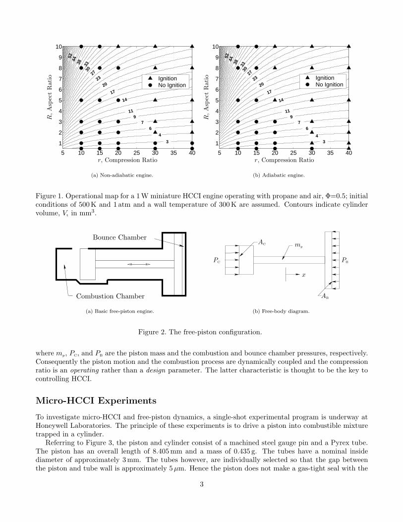
Aichlmayr et al. [28] used detailed chemical kinetics and conduction heat transfer to explore the physicallimitations of HCCI combustion in a slider-crank engine configuration. Aichlmayr et al. first used perfor-mance estimation to establish engine designs and then used detailed kinetics to determine whether or notHCCI was compatible with the given conditions. Results for 1 W engines are presented in Figure 1. Theyindicate that small HCCI engines are possible and that heat transfer is a serious physical limitation. Fur-ther analyses conducted with the power output constrained to be 10W and 0.1W reveal that heat transferbecomes increasingly significant when the engine characteristic dimension decreases—a result consistentwith Eq. (1).

Free-Piston Engines

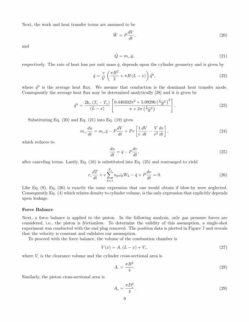
Although HCCI is arguably a good match for micro-engines, ignition timing is a problem. One possiblesolution is a free-piston configuration [29–31] like that depicted in Figure 2(a)1. Note that the pistonmotion depends exclusively upon gas forces (Figure 2(b)) i.e.,

ΣFx = mp

d2x

dt2= PCAC − PBAB, (2)

1Note that a counterbalancing mechanism, work extraction scheme, and a scavenging pump are omitted for clarity of the figure andbrevity of the discussion.

2

5 10 15 20 25 30 35 40

1

2

3

4

5

6

7

8

9

10

5244

38 3330

27

23

20

17

14

11

76

4

3

9

Ignition No Ignition

r, Compression Ratio

R,A

spec

tR

atio

(a) Non-adiabatic engine.

5 10 15 20 25 30 35 40

1

2

3

4

5

6

7

8

9

10

5244

38 3330

27

23

20

17

14

11

76

43

9

Ignition No Ignition

r, Compression Ratio

R,A

spec

tR

atio

(b) Adiabatic engine.

Figure 1. Operational map for a 1W miniature HCCI engine operating with propane and air, Φ=0.5; initialconditions of 500K and 1 atm and a wall temperature of 300K are assumed. Contours indicate cylindervolume, Vt in mm3.

Bounce Chamber

Combustion Chamber

(a) Basic free-piston engine.

mp

AB

AC

PC PB

x

(b) Free-body diagram.

Figure 2. The free-piston configuration.

where mp, PC, and PB are the piston mass and the combustion and bounce chamber pressures, respectively.Consequently the piston motion and the combustion process are dynamically coupled and the compressionratio is an operating rather than a design parameter. The latter characteristic is thought to be the key tocontrolling HCCI.

Micro-HCCI Experiments

To investigate micro-HCCI and free-piston dynamics, a single-shot experimental program is underway atHoneywell Laboratories. The principle of these experiments is to drive a piston into combustible mixturetrapped in a cylinder.

Referring to Figure 3, the piston and cylinder consist of a machined steel gauge pin and a Pyrex tube.The piston has an overall length of 8.405mm and a mass of 0.435 g. The tubes have a nominal insidediameter of approximately 3mm. The tubes however, are individually selected so that the gap betweenthe piston and tube wall is approximately 5µm. Hence the piston does not make a gas-tight seal with the

3

8.405 mm

3 mm

L

End PlugCompressed Air Pyrex TubePiston

Injector PinHammer

Figure 3. Single-Shot Experimental Setup

tube. Also, the length of the tube, L ranges from approximately 25mm to 57 mm. The end of the cylinderis sealed with a removable plug and three O-rings. Finally, compressed air released by a solenoid-actuatedvalve is used to accelerate the hammer. The hammer subsequently strikes the injector pin and impulsesthe piston.

Time-resolved measurements of piston velocity and position are obtained from movies recorded by aVision Research Phantom v4.0 digital camera. The camera is configured to begin acquisition with theactuation of the compressed-air valve and the maximum exposure and sampling rates are 100, 000 frames

s

and 62, 500 Pixelss , respectively. These settings yield a temporal resolution of 16µs. The spatial resolution

depends upon the camera position and varies from 0.1mm to 0.4mm.Charge preparation consists of drawing a heptane-air mixture from a bubbler into a syringe. The

equivalence ratio is varied by replacing a given volume of mixture in the syringe with ambient air. Thistechnique yields equivalence ratios from 0.25 to 2.9.

The single-shot experiment proceeds as follows: First, the end plug is removed and the hammer, injectorpin, piston, and camera are placed in their “ready” states. Next, a fuel-air mixture is injected into thecylinder and the end plug is inserted. Finally, the compressed air valve is actuated.

Results

A typical single-shot image sequence is presented in Figure 4. Here the equivalence ratio is 0.69, L=57mm,the initial velocity is 41 m

s , and the final velocity is 49 ms . Combustion is indicated by the optical emission

and one should note that the piston is nearly stationary when the explosion occurs. Consequently thisarrangement closely approximates an Otto cycle [29]. But more importantly, the images in Figure 4demonstrate that micro-combustion with a large alkane can be achieved in a space approximately 3mmin diameter and 0.3mm wide without having to employ catalysts, an external ignition system, heating thewalls, or preheating the charge.

Additionally, a hallmark of HCCI is the ability to ignite extremely lean mixtures. A sensible questionto ask would be: “Does this hold for micro-combustion?” According to Figure 5 where the equivalenceratio is 0.25, it does. Moreover, Figure 5 suggests that ignition commences at the center of the combustionchamber and that the charge is consumed through a series of explosions.

4

Image Comments

Compression stroke, t = t0. Distance be-tween piston and end plug: 1.1 mm.

Compression stroke, t = t0 + 16µs. Distancebetween piston and end plug: 0.5 mm.

Ignition, t = t0 + 32µs. Distance betweenpiston and end plug: 0.3 mm.

Combustion and beginning of the expansionstroke, t = t0 + 64µs. Distance between pis-ton and end plug: 0.5 mm.

Expansion stroke, t = t0 + 96µs. Distancebetween piston and end plug: 0.8 mm.






Expansion stroke and end of combustion, t =t0 +288µs. Distance between piston and endplug: 3.9 mm.

Figure 4. A typical sequence of images from a single-shot experiment. The fuel is n-heptane and theequivalence ratio is 0.69. Also, the charge was initially at room temperature and pressure. Refer toFigure 3 for additional dimensions (L=57mm).

5

Image Comments

Compression stroke, t = t0. Distance be-tween piston and end plug: 1.7 mm.





Combustion and beginning of the expansionstroke, t = t0 + 128µs. Distance betweenpiston and end plug: 0.7 mm.





Expansion stroke and end of combustion, t =t0 +288µs. Distance between piston and endplug: 2.9 mm.

Figure 5. A typical sequence of images from a single-shot experiment. The fuel is n-heptane and theequivalence ratio is 0.25. Also, the charge was initially at room temperature and pressure. Refer toFigure 3 for additional dimensions (L=57mm).

6

Modeling the Single-Shot Experiments

To explore the coupling of free-piston dynamics and HCCI combustion, a numerical model of the single-shotexperiments is developed. A schematic of the physical system is presented in Figure 6 and the followingis assumed: 1. Temperature, pressure, and species concentrations are uniform., 2. The gas escaping

L

T∞

P∞

mp

V (t)

v(t)

xDp

B

T (t)

P (t)

Yk(t)

Figure 6. Schematic for single-shot model formulation (dashed-line indicates the control surface).

through the piston-cylinder gap (leakage or blow-by) may be described by one-dimensional quasi-steadycompressible flow., 3. The compression process is quasi-static., 4. Compressibility effects within thecombustion chamber are negligible., and 5. Conduction is the dominant heat transfer mode. The model isdeveloped by applying mass, energy, and force balances and proceeds as follows:

Mass Balance

A mass balance applied to the control volume gives:

dmcv

dt+ m = 0. (3)

where m is the mass flow rate of escaping gas. Alternatively, Eq. (3) may be expressed in terms of thecylinder volume V , and specific volume v, by making the substitution mcv=V

v . The results is

1v

dV

dt− V

v2

dv

dt+ m = 0. (4)

Also, the blow-by mass flow rate is assumed to be given by

m =CdAtP

(RmT )12

M (P, P∞, γ) , (5)

where

M (P, P∞, γ) =

(P∞P

) 1γ

{2γ

γ−1

[1 − (

P∞P

) γ−1γ

]} 12 P∞

P >(

2γ+1

) γ

γ−1

γ12

(2

γ+1

) γ+12(γ−1) P∞

P ≤(

2γ+1

) γ

γ−1. (6)

A mass balance on species k yields

dmk

dt= mk

′′′V − mk, (7)

where mk′′′ is the volumetric rate of creation of species k. Next, if one assumes that mk=mYk and

substitutes mk=Ykmcv and mk′′′=ωkWk into Eq. (7), then

mcv

dYk

dt= ωkWkV − Yk

[m +

dmcv

dt

]. (8)

7

The quantity in square brackets however, is Eq. (3). Thus Eq. (8) reduces to

dYk

dt= vωkWk, (9)

which interestingly, is exactly the same expression that one would obtain if leakage had been neglected.

Energy Balance

An energy balance applied to the control volume gives:

dUcv

dt= Q − W − mh. (10)

Next, Ucv=mcvu and

u =Ns∑

k=1

ukYk, (11)

are differentiated to yield

dUcv

dt= mcv

du

dt+ u

dmcv

dt, (12)

and

du

dt=

Ns∑k=1

ukdYk

dt+

Ns∑k=1

Ykduk

dt, (13)

respectively. Then

uk = cvkT, (14)

is differentiated and substituted into Eq. (13) along with

cv =Ns∑

k=1

cvkYk, (15)

and Eq. (9). The result is

du

dt= v

Ns∑k=1

ukωkWk + cv

dT

dt. (16)

Eq. (10) and Eq. (12) are used to eliminate dUcvdt , i.e.,

mcv

du

dt= Q − W − mh − u

dmcv

dt. (17)

But when Eq. (3) is substituted for m, we have

mcv

du

dt= Q − W + (h − u)

dmcv

dt, (18)

which in turn, reduces to

mcv

du

dt= Q − W + Pv

dmcv

dt. (19)

8

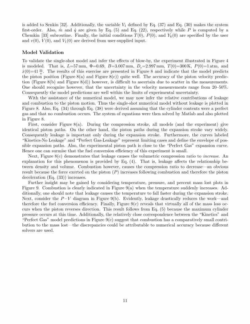
Next, the work and heat transfer terms are assumed to be

W = PdV

dt, (20)

and

Q = mcvq, (21)

respectively. The rate of heat loss per unit mass q, depends upon the cylinder geometry and is given by

q =v

V

(πB2

2+ πB (L − x)

)¯q′′, (22)

where ¯q′′ is the average heat flux. We assume that conduction is the dominant heat transfer mode.Consequently the average heat flux may be determined analytically [28] and it is given by

¯q′′ =2kT (T0 − Tw)

(L − x)

[0.440332π2 + 5.09296

(L−xB

)2

π + 2π(

L−xB

)]

. (23)

Substituting Eq. (20) and Eq. (21) into Eq. (19) gives

mcv

du

dt= mcvq − P

dV

dt+ Pv

[1v

dV

dt− V

v2

dv

dt

], (24)

which reduces todu

dt= q − P

dv

dt, (25)

after canceling terms. Lastly, Eq. (16) is substituted into Eq. (25) and rearranged to yield

cv

dT

dt+ v

Ns∑k=1

ukωkWk − q + Pdv

dt= 0. (26)

Like Eq. (9), Eq. (26) is exactly the same expression that one would obtain if blow-by were neglected.Consequently Eq. (4) which relates density to cylinder volume, is the only expression that explicitly dependsupon leakage.

Force Balance

Next, a force balance is applied to the piston. In the following analysis, only gas pressure forces areconsidered, i.e., the piston is frictionless. To determine the validity of this assumption, a single-shotexperiment was conducted with the end plug removed. The position data is plotted in Figure 7 and revealsthat the velocity is constant and validates our assumption.

To proceed with the force balance, the volume of the combustion chamber is

V (x) = Ac (L − x) + Vc, (27)

where Vc is the clearance volume and the cylinder cross-sectional area is

Ac =πB2

4. (28)

Similarly, the piston cross-sectional area is

Ap =πD2

p

4. (29)

9

0 0.5 1 1.5

0.5

1

1.5

2

2.5

3

3.5

4Data Linear Fit

Pos

itio

n(c

m)

Time (ms)

Figure 7. Position data from a single-shot experiment with the end plug removed. The slope of the fittedline is −29.5 m

s .

Next, Eq. (27) is differentiated twice to yield

dV

dt= −Ac

dx

dt(30)

and

d2V

dt2= −Ac

d2x

dt2. (31)

Consequently a force balance on the piston, viz.

mp

d2x

dt2= Ap (P∞ − P ) , (32)

may be expressed in terms of the cylinder volume by substituting Eq. (32) into Eq. (31), i.e.,

d2V

dt2= −AcAp (P∞ − P )

mp

. (33)

Model Implementation

To implement the single-shot model, a “reactor problem” consisting of the following equations:

dT

dt=

q

cv

− P

cv

dv

dt− v

cv

Ns∑k=1

ukωkWk, (34)

dYk

dt= vωkWk, (35)

dV1

dt= −AcAp (P∞ − P )

mp

, (36)

dV

dt= V1, (37)

dv

dt=

v2

Vm +

v

VV1, (38)

10

is added to Senkin [32]. Additionally, the variable V1 defined by Eq. (37) and Eq. (30) makes the systemfirst-order. Also, m and q are given by Eq. (5) and Eq. (22), respectively while P is computed by aChemkin [33] subroutine. Finally, the initial conditions T (0), P (0), and Yk(0) are specified by the userand v(0), V (0), and V1(0) are derived from user-supplied input.

Model Validation

To validate the single-shot model and infer the effects of blow-by, the experiment illustrated in Figure 4is modeled. That is, L=57mm, Φ=0.69, B=3.007mm, Dp=2.997mm, T (0)=300K, P (0)=1 atm, andx(0)=41 m

s . The results of this exercise are presented in Figure 8 and indicate that the model predictsthe piston position (Figure 8(a) and Figure 8(c)) quite well. The accuracy of the piston velocity predic-tion (Figure 8(b) and Figure 8(d)) however, is difficult to ascertain due to scatter in the measurements.One should recognize however, that the uncertainty in the velocity measurements range from 20–50%.Consequently the model predictions are well within the limits of experimental uncertainty.

With the assistance of the numerical model, we may now infer the relative contributions of leakageand combustion to the piston motion. Thus the single-shot numerical model without leakage is plotted inFigure 8. Also, Eq. (34) through Eq. (38) were derived assuming that the cylinder contents were a perfectgas and that no combustion occurs. The system of equations were then solved by Matlab and also plottedin Figure 8.

First, consider Figure 8(a). During the compression stroke, all models (and the experiment) giveidentical piston paths. On the other hand, the piston paths during the expansion stroke vary widely.Consequently leakage is important only during the expansion stroke. Furthermore, the curves labeled“Kinetics-No Leakage” and “Perfect Gas-Leakage” represent limiting cases and define the envelope of pos-sible expansion paths. Also, the experimental piston path is close to the “Perfect Gas” expansion curve.Hence one can surmise that the fuel conversion efficiency of this experiment is small.

Next, Figure 8(c) demonstrates that leakage causes the volumetric compression ratio to increase. Anexplanation for this phenomenon is provided by Eq. (4). That is, leakage affects the relationship be-tween density and volume. Combustion however, causes the compression ratio to decrease—an obviousresult because the force exerted on the piston (P ) increases following combustion and therefore the pistondeceleration (Eq. (33)) increases.

Further insight may be gained by considering temperature, pressure, and percent mass lost plots inFigure 9. Combustion is clearly indicated in Figure 9(a) when the temperature suddenly increases. Ad-ditionally, one should note that leakage causes the temperature to fall faster during the expansion stroke.Next, consider the P−V diagram in Figure 9(b). Evidently, leakage drastically reduces the work—andtherefore the fuel conversion efficiency. Finally, Figure 9(c) reveals that virtually all of the mass loss oc-curs when the piston reverses direction. This result follows from Eq. (5) because the maximum cylinderpressure occurs at this time. Additionally, the relatively close correspondence between the “Kinetics” and“Perfect Gas” model predictions in Figure 9(c) suggest that combustion has a comparatively small contri-bution to the mass lost—the discrepancies could be attributable to numerical accuracy because differentsolvers are used.

11

0 0.5 1 1.5 2 2.5 30

1

2

3

4

5

6

Experiment Kinetics−Leakage Kinetics−No Leakage Perfect Gas−Leakage Perfect Gas−No Leakage

Pos

itio

n(c

m)

Time (ms)

(a) Piston position measurements and predictions.

0 0.5 1 1.5 2 2.5 3 3.5

−60

−40

−20

0

20

40 Kinetics−Leakage Kinetics−No Leakage Perfect Gas−Leakage Perfect Gas−No LeakageExperiment

Vel

ocity

(ms)

Time (ms)

(b) Piston velocity measurements and predictions.

1.3 1.4 1.5 1.6 1.7 1.84.8

4.9

5

5.1

5.2

5.3

5.4

5.5

5.6

5.7

5.8

Experiment Kinetics−Leakage Kinetics−No Leakage Perfect Gas−Leakage Perfect Gas−No Leakage

Pos

itio

n(c

m)

Time (ms)

(c) Closeup piston position measurements and predic-tions.

0.6 0.8 1 1.2 1.4 1.6 1.8

−60

−50

−40

−30

−20

−10

0

10

20

30

40

Kinetics−Leakage Kinetics−No Leakage Perfect Gas−Leakage Perfect Gas−No LeakageExperiment

Vel

ocity

(ms)

Time (ms)

(d) Closeup piston velocity measurements and predictions.

Figure 8. A comparison of experimental data obtained from the images shown in Figure 4 and varioussingle-shot models. Errorbars are omitted for clarity, but uncertainties in position, time, and velocity are0.1mm, 16µs, and 20–50%, respectively.

12

1.4 1.5 1.6 1.7 1.8 1.9

500

1000

1500

2000

2500

3000Kinetics−Leakage Kinetics−No Leakage Perfect Gas−Leakage Perfect Gas−No Leakage

Time (ms)

Tem

pera

ture

(K)

(a) Temperature histories obtained from various single-shot models.

10−3

10−2

10−1

100

100

101

102

103

Leakage No Leakage

Volume(cm3

)P

ress

ure

(atm

)

(b) Pressure-Volume diagrams obtained from leakage and

non-leakage models (kinetics only).

0 0.5 1 1.5 2 2.50

10

20

30

40

50

60 Kinetics Perfect Gas

Time (ms)

Per

cent

Mas

sLos

t

(c) Percent mass lost predicted by the kinetics and perfectgas models.

Figure 9. Predicted temperature, P-V diagrams, and percent mass lost corresponding to the conditionsunder which the images in Figure 4 were obtained.

13

Parametric Study

To further explore the effects of initial velocity, chamber length, equivalence ratio, and fuel type on leakageand indicated efficiency, a parametric study is conducted. The parameters considered and their values arepresented in Table 1.

Table 1. Parametric study inputs.Parameter Value(s) UnitInitial Velocity 5, 10, 15, 20, 25, 30, 35, 40, 45, 50 m

sChamber Length (L) 0.6, 1.5, 3.0, 4.5, 7.5, 9.0 cmEquivalence ratio (Φ) 0.25, 0.47, 0.69, 0.95, 1.5, 2.9 NAFuel (Kinetic Mechanism) Heptane [34] and Propane [35] NADischarge Coefficient (Cd) 0.0 and 1.0 NAInitial Temperature 300 KInitial Pressure 1 atmPiston Mass (mp) 0.431 gClearance Volume (Vc) 0.71591E-03 cm3

Piston Diameter (Dp) 0.29972 cmCylinder Bore (B) 0.300228 cmWall Temperature (Tw) 300 K

First, the effect of the chamber length on leakage is investigated in Figure 10. One should note that

0 2 4 6 8 1025

30

35

40

45

50

55

60

65V=20 m/sV=25 m/sV=30 m/sV=35 m/sV=40 m/sV=45 m/sV=50 m/s

Per

cent

Mas

sLos

t

Chamber Length, L (cm)

(a) Φ=0.95

0 2 4 6 8 1025

30

35

40

45

50

55

60

65V=30 m/sV=35 m/sV=40 m/sV=45 m/sV=50 m/s

Per

cent

Mas

sLos

t

Chamber Length, L (cm)

(b) Φ=0.25

Figure 10. Percent mass lost versus chamber length, L; open symbols indicate heptane-air and dark symbolsindicate propane-air.

both heptane-air and propane-air cases having Φ=0.95 are plotted in Figure 10(a) and even though theinitial velocity and fuel are varied, a relationship between the chamber length and mass lost clearly exists.Further weight is given to this supposition in Figure 10(b) where the results of the various runs almostperfectly coincide.

Next, the relationship between the indicated fuel conversion efficiency and compression ratio is illus-trated in Figure 11. By examining Figure 11, the assertion that the combination of HCCI and a free-pistonis a close approximation to an Otto cycle may be tested. The “ideal” cases, i.e., no leakage, are presented

14

in Figure 11(b), Figure 11(d), and Figure 11(f). Evidently, the model predicts that Otto cycle efficiencymay be achieved. This is an expected result because the P−V diagrams resemble Figure 9(b), which inturn, resembles the Otto cycle. Furthermore, a few cases in Figure 11(d) and Figure 11(f) exceed the Ottocycle efficiency. This “impossible” result however, is a consequence of assuming γ=1.3.

Next, Figure 11 demonstrates that leakage drastically reduces the indicated efficiency. This result isalso expected from Figure 9(b). Additionally, the peak efficiencies for Figure 11(a), Figure 11(c), andFigure 11(e) appear to decrease with the equivalence ratio. Whereas Figure 11(b), Figure 11(d), andFigure 11(f) exhibit the opposite trend. Also, when leakage is considered, the maximum efficiencies occurbetween r=50 and r=100. On the other hand, the efficiency continues to increase until approximatelyr=150 when leakage is not considered.

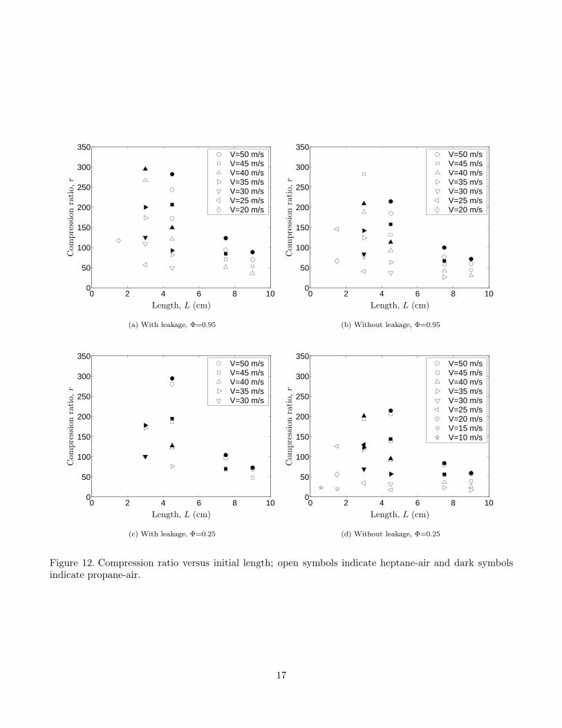
The compression ratio varies with the initial conditions of the problem. To demonstrate, the compressionratio for various chamber lengths, initial velocities, equivalence ratios, and fuels are plotted in Figure 12.The effect of leakage is apparent by comparing Figure 12(a) and Figure 12(b). That is, leakage causes thecompression ratio to increase. Moreover, this increase depends strongly upon the chamber length. Butthis result is expected because leakage varies inversely with the chamber length (Figure 10).

Figure 12 also indicates that the compression ratio depends upon the initial velocity. That is, the greaterthe velocity, the greater the compression ratio—an intuitive result. Alternatively, Figure 12 demonstratesthat the compression ratio becomes increasingly sensitive to the initial velocity when the chamber lengthdecreases.

Finally, by comparing heptane-air and propane-air cases in Figure 12, one should note that for identicalinitial velocities and chamber lengths, the propane-air cases have greater compression ratios. Further, ifone compares Figure 12(b) and Figure 12(d), one should note that the differences in the compression ratiosnearly disappears. A γ dependence is a possible explanation for this phenomena.

15

0 50 100 150 200 250 3000

20

40

60

80

100Otto L=9.0 cmL=7.5 cmL=4.5 cmL=3.0 cmL=1.5 cm

η fc,i,Per

cent

Compression ratio, r

(a) With leakage, Φ=0.95

0 50 100 150 200 250 3000

20

40

60

80

100

Otto L=9.0 cmL=7.5 cmL=4.5 cmL=3.0 cmL=1.5 cm

η fc,i,Per

cent


(b) Without leakage, Φ=0.95

0 50 100 150 200 250 3000

20

40

60

80

100

Otto L=9.0 cmL=7.5 cmL=4.5 cmL=3.0 cm

η fc,i,Per

cent


(c) With leakage, Φ=0.47

0 50 100 150 200 250 3000

20

40

60

80

100

Otto L=9.0 cmL=7.5 cmL=4.5 cmL=3.0 cmL=1.5 cm

η fc,i,Per

cent


(d) Without leakage, Φ=0.47

0 50 100 150 200 250 3000

20

40

60

80

100

Otto L=9.0 cmL=7.5 cmL=4.5 cmL=3.0 cm

η fc,i,Per

cent


(e) With leakage, Φ=0.25

0 50 100 150 200 250 3000

20

40

60

80

100

Otto L=9.0 cmL=7.5 cmL=4.5 cmL=3.0 cmL=1.5 cmL=0.6 cm

η fc,i,Per

cent


(f) Without leakage, Φ=0.25

Figure 11. Indicated fuel conversion efficiency versus compression ratio; open symbols indicate heptane-airand dark symbols indicate propane-air. The Otto cycle efficiency is computed by assuming γ=1.3.

16

0 2 4 6 8 100

50

100

150

200

250

300


Com

pres

sion

rati

o,r

Length, L (cm)

(a) With leakage, Φ=0.95

0 2 4 6 8 100

50

100

150

200

250

300


Com

pres

sion

rati

o,r

Length, L (cm)

(b) Without leakage, Φ=0.95

0 2 4 6 8 100

50

100

150

200

250

300

350V=50 m/sV=45 m/sV=40 m/sV=35 m/sV=30 m/s

Com

pres

sion

rati

o,r

Length, L (cm)

(c) With leakage, Φ=0.25

0 2 4 6 8 100

50

100

150

200

250

300

350V=50 m/sV=45 m/sV=40 m/sV=35 m/sV=30 m/sV=25 m/sV=20 m/sV=15 m/sV=10 m/s

Com

pres

sion

rati

o,r

Length, L (cm)

(d) Without leakage, Φ=0.25

Figure 12. Compression ratio versus initial length; open symbols indicate heptane-air and dark symbolsindicate propane-air.

17

Non-Dimensional Analysis

To better understand the influence of the various model parameters on leakage and the compression ratio,the governing equations are non-dimensionalized. Let

V ∗ =V

V0, t∗ =

t

τ, v∗ =

v

v0, T ∗ =

T

T0, and P ∗ =

P

P0. (39)

Where V0, v0, T0, and P0 are the initial values of V , v, T , and P , respectively and τ is a characteristictime. The non-dimensional forms of Eq. (9), Eq. (26), Eq. (4), Eq. (30), and Eq. (31) are then given by

dYk

dt∗= v∗v0τ ωkWk, (40)

dT ∗

dt∗+

v0τ

cvT0v∗

Ns∑k=1

ukωkWk − qτ

cvT0+

P0v0

cvT0P ∗dv∗

dt∗= 0, (41)

dv∗

dt∗=

τv0m

V0

v∗2

V ∗ +v∗

V ∗dV ∗

dt∗, (42)

dV ∗

dt∗= − xτ

LRmax

, (43)

and

d2V ∗

dt∗2 =τ2P∞

LRmax

(mp

Ap

) (P ∗ − 1) , (44)

respectively when P0=P∞ and T0=T∞ is assumed. Also

Rmax =rcyl

rcyl − 1, (45)

where rcyl=V0Vc

, is the maximum compression ratio of the cylinder.

Leakage

The non-dimensional blow-by mass flow rate is

τv0m

V0=

(At

Ac

)τv0P0CdM (P0P

∗, P0, γ)

L (RmT0)12 Rmax

(P ∗

T ∗ 12

). (46)

Next,

At

Ac

=(

tGDp

) 4(

tG

Dp

)+ 4

4(

tG

Dp

)2+ 4

(tG

Dp

)+ 1

, (47)

or

At

Ac

≈ 4(

tGDp

), (48)

when ratio of the gap length tG, to the piston diameter Dp, is small. Hence

τv0m

V0≈ 4

(tGDp

){τv0P0CdM (P0P

∗, P0, γ)

L (RmT0)12 Rmax

} (P ∗

T ∗ 12

). (49)

18

Eq. (49) implies that the gap to piston diameter ratio and the chamber length strongly influence the blow-by mass flow rate. This implication is supported by Figure 10. On the other hand, the influence of tG

Dpwas

not explored in the parametric analysis, but anecdotal evidence confirms that leakage is very sensitive toit.

Therefore to reduce leakage one must: (1) Increase the cylinder length., (2) Increase the piston diameter.,or (3) Decrease the gap width. The minimum gap width however, is fixed by the fabrication method.Consequently an increase in leakage is generally an unavoidable consequence of reducing either the pistondiameter or stroke.

Compression Ratio

Next, Eq. (43) and Eq. (44) describe the piston motion, but depend upon a characteristic time. The cycletime is a logical choice, but it cannot be determined a priori. Therefore the “half-cycle” time is usedinstead. Let

dV ∗

dt∗

∣∣∣∣t∗=0

= − x0τ

LRmax

= −1, (50)

where x0=x(0). Consequently τ=LRmaxx0

is the half-cycle time and substitution into Eq. (44) yields

d2V ∗

dt∗2 =LRmaxP∞x2

0

(mp

Ap

) (P ∗ − 1) . (51)

Hence

Γ =LRmaxP∞x2

0

(mp

Ap

) , (52)

is possibly an important non-dimensional parameter because the non-dimensional volume, V ∗ is the inverseof the instantaneous compression ratio, r. To explore this possibility, results from the parametric study areplotted in Figure 13. They suggest that r is indeed a function of Γ. Moreover, because the various casesconsidered in Figure 13 yield essentially the same curve, the relationship between r and Γ appears to beonly mildly sensitive to leakage and γ. This result however, is expected because the various predictions forthe piston position during the compression stroke in Figure 8(a) and Figure 8(c), are essentially the same.

Furthermore, one may rearrange Eq. (52) to yield

Γ =LApP∞Rmax

mpx20

. (53)

However Rmax≈1 and LAp is the maximum volume that can be swept by the piston. Consequently P∞ApLis the work required to displace this volume of gas. Hence

Γ =Work required to displace the volume swept by the piston

2 × Kinetic energy of the piston. (54)

Alternatively, the initial kinetic energy of the piston is equal to the compression work because the pistonis brought to rest.

Consequently if one assumes from Figure 11 that 50≤r≤100 maximizes efficiencies, then Figure 13implies that 0.45≤Γ≤0.7. Thus

2.2 ≥ 1Γ

≥ 1.4, (55)

or

1.1 ≥ Kinetic energy of the pistonWork required to displace the volume swept by the piston

≥ 0.7, (56)

is optimal.

19

10−2

10−1

100

101

100

101

102

103

L=9.0 cmL=7.5 cmL=4.5 cmL=3.0 cmL=1.5 cm

Com

pres

sion

rati

o,r

Dynamic Parameter, Γ

(a) Heptane-air, Φ=0.95

10−2

10−1

100

101

100

101

102

103


Com

pres

sion

rati

o,r


(b) Propane-air, Φ=0.95

10−2

10−1

100

101

100

101

102

103


Com

pres

sion

rati

o,r


(c) Heptane-air, Φ=0.25

10−1

100

101

100

101

102


Com

pres

sion

rati

o,r


(d) Propane-air, Φ=0.25

Figure 13. Compression ratio versus dynamics parameter, Γ for heptane-air and propane-air charges havingequivalence ratios of Φ=0.95 and Φ=0.25; open symbols indicate cases with leakage.

20

Conclusions and Future Work

This paper presents results from micro-HCCI experiments and a detailed chemical kinetic model. Also,the relationship between model (or experiment) parameters on leakage and the compression ratio areexplored via a parametric model study and non-dimensionalization of the governing equations. Finally, anon-dimensional parameter that relates initial conditions to the compression ratio is proposed.

The salient findings of this paper include:

• HCCI is possible in spaces 3mm diameter and 0.3mm long.

• HCCI combustion with equivalence ratios of Φ=0.69 and Φ=0.25 is demonstrated.

• A model which couples free-piston motion and detailed chemical kinetics is developed and used tomodel the single-shot micro-HCCI experiments.

• Sliding friction in the single-shot experiments is negligible.

• The single-shot numerical model employing detailed chemical kinetics is shown to reproduce pistonposition and velocity measurements very well.

• Leakage (blow-by) accounts for:

– A distortion of the piston-time path during the expansion stroke.

– A decrease in the final velocity of the piston.

– An increase in the compression ratio relative to an ideal case.

– A decrease in the fuel conversion efficiency.

– A reversal of the fuel conversion efficiency versus equivalence ratio relationship relative to anideal case.

• Leakage may be reduced by:

– Increasing the chamber length, L.

– Decreasing the gap to piston diameter ratio, tG

Dp.

• The non-dimensional parameter defined by Eq. (52):

– Appears to capture the relationship between initial conditions and the compression ratio.

– May be interpreted to be the ratio of “The work required to displace the volume swept by thepiston to the kinetic energy of the piston.”

– If one assumes that a compression ratio between 50 and 100 is optimal, then the piston mass,initial velocity, and cylinder length must satisfy the constraint 0.45≤Γ≤0.7.

In the future, further parametric studies will be conducted to clarify the relationship between Γ andthe compression ratio. Also, the relationship between leakage and the initial conditions will be furtherexplored and strategies to minimize leakage will be devised. Finally, the coupling between piston dynamicsand chemical kinetics will be analyzed in detail to elucidate conditions necessary for ignition.

Acknowledgement

This project was sponsored by Honeywell International under DARPA contract No. F30602-99-C-0200.Also, the authors wish to thank Dr. Wei Yang and Mr. Tom Rezachek of Honeywell International.

21

Nomenclature

AB Bounce piston area(m2

), Eq. (2).

AC Combustion piston area(m2

), Eq. (2).

Ac Cylinder area(m2

), Eq. (28).

Ap Piston face area(m2

), Eq. (29).

As Surface area(m2

), Eq. (1).

At Gap area, At=π4

(B2 − D2

p

) (m2

), Eq. (5).

As

VSurface area to volume ratio

(1m

), Eq. (1).

B Cylinder bore (mm).

Cd Discharge coefficient (unitless), Eq. (5).

Dp Piston diameter (mm).

Fx x-Direction force (N), Eq. (2).

L Initial distance between piston and end plug (mm).

Ns Total number of species (unitless), Eq. (15).

P Pressure (atm), Eq. (5).

PB Bounce chamber pressure (atm), Eq. (2).

PC Combustion chamber pressure (atm), Eq. (2).

P ∗ Non-dimensional pressure (unitless), Eq. (39).

P∞ Ambient pressure (atm), Eq. (5).

P0 Initial pressure (atm), Eq. (39).

Q Heat transfer rate (W), Eq. (1).

R Stroke-to-bore aspect ratio (unitless).

Rm Mixture gas constant(

kJkgK

), Eq. (5).

Rmax Ratio defined by Rmax=rcyl

rcyl−1 (unitless), Eq. (45).

T Temperature (K), Eq. (5).

T ∗ Non-dimensional temperature (unitless), Eq. (39).

T∞ Ambient temperature (K).

T0 Initial temperature (K), Eq. (39).

Ucv Internal energy of the control volume (kJ), Eq. (10).

V Volume(m3

), Eq. (4).

V Volume(m3

), Eq. (1).

22

V ∗ Non-dimensional cylinder volume (unitless), Eq. (39).

V1 Variable defined by Eq. (37),(

m3

s

)Vc Clearance volume

(m3

), Eq. (27).

Vt Total cylinder volume(mm3

).

V0 Initial volume(m3

), Eq. (39).

W Rate of work done on the control volume (W), Eq. (10).

Wk Molecular weight of species k( g

mol

), Eq. (9).

Yk Mass fraction of species k (unitless).

cv Specific heat(

kJkgK

), Eq. (15).

cvk Specific heat of species k(

kJkgK

), Eq. (14).

h Specific enthalpy(

kJkg

), Eq. (10).

kT Thermal conductivity(

WmK

), Eq. (23).

m Mass of material (kg), Eq. (1).

m Mass flow rate of escaping gas(

kgs

), Eq. (3).

mcv Mass of the control volume (kg), Eq. (3).

mk Mass of species k (kg), Eq. (7).

mk Mass flow rate of species k(

kgs

), Eq. (7).

mk′′′ Mass volumetric rate of creation of species k

(kgm3

), Eq. (7).

mp Piston mass (kg), Eq. (2).

q Specific heat transfer rate(

Wkg

), Eq. (1).

q′′ Heat flux(

Wm2

), Eq. (1).

¯q′′ Average heat flux(

Wm2

), Eq. (1).

r Volumetric compression ratio (unitless).

rcyl Maximum geometric compression ratio, rcyl=V0Vc

(unitless), Eq. (45).

t Time (s), Eq. (2).

t∗ Non-dimensional time (unitless), Eq. (39).

tG Piston-cylinder gap, tG=B−Dp

2 , (mm), Eq. (47).

u Specific internal energy(

kJkg

), Eq. (12).

23

uk Specific internal energy of species k(

kJkg

), Eq. (15).

v Specific volume(

m3

kg

), Eq. (4).

v∗ Non-dimensional specific volume (unitless), Eq. (39).

v0 Initial specific volume(

kgm3

), Eq. (39).

x Cartesian coordinate (m), Eq. (2).

x Shorthand for dxdt

(ms

), Eq. (42).

x0 Initial piston velocity(

ms

), Eq. (50).

Γ Free-piston dynamic parameter (unitless), Eq. (52).

Φ Fuel-air equivalence ratio (unitless).

γ Specific heat ratio (unitless), Eq. (5).

ρ Density(

kgm3

), Eq. (1).

ρ Average density(

kgm3

), Eq. (1).

τ Characteristic time (s), Eq. (39).

24

References

[1] Peterson, R. B. Small packages. Mechanical Engineering 123(6) pp. 58–61 (2001).[2] Yang, W., Bonne, U., et al. MEMS free-piston knock engine. Technical Proposal, DARPA Contract

F30602-99-C-0200 (1999). Honeywell Technology Center, 12001 State Highway 55, Plymouth, MN55441.

[3] Epstein, A. H., Senturia, S. D., Anathasuresh, G., Ayon, A., Breuer, K., Chen, K., Ehrich, F. E.,Gauba, G., Ghodssi, R., Groshenry, C., Jacobson, S., Lang, J. H., Lin, C., Mehra, A., Miranda, J. M.,Nagle, S., Orr, D. J., Piekos, E., Schmidt, M. A., Shirley, G., Spearing, M. S., Tan, C. S., Tzeng, Y.,and Waitz, I. A. Power MEMS and microengines. In Transducers ’97 Chicago : digest of technicalpapers, pp. 753–756. IEEE, Chicago, Ill (1997).

[4] Fernandez-Pello, C., Liepmann, D., Pisano, A., et al. MEMS rotary combustion laboratories.University of California at Berkeley Internet Document (Last loaded July 2001) (2001). URLhttp://www.me.berkeley.edu/mrcl/.

[5] Yang, W., Bonne, U., and Johnson, B. R. Microcombustion engine/generator. U. S. Patent 6,276,313(2001).

[6] Allen, M. et al. Research topics–miniature MEMS free-piston engine generator. Georgia Institute ofTechnology Internet Document (Last loaded July 2001) (2001). URL http://comblab5.ae.gatech.edu/Minipiston/intro.htm.

[7] Waitz, I. A., Gauba, G., and Tzeng, Y. Combustors for Micro-Gas Turbine Engines. Journal of FluidsEngineering 120(1) pp. 109–117 (1998).

[8] Onishi, S., Jo, S. H., Shoda, K., Jo, P. D., and Kato, S. Active thermo-atmosphere combustion(ATAC)–a new combustion process for internal combustion engines. SAE Technical Paper 790501(1979).

[9] Najt, P. M. and Foster, D. E. Compression-ignited homogeneous charge combustion. SAE TechnicalPaper 830264 (1983).

[10] Iida, N. Combustion analysis of methanol-fueled active thermo-atmosphere combustion (ATAC) engineusing a spectroscopic observation. SAE Technical Paper 940684 (1994).

[11] Lavy, J., Duret, P., Habert, P., Esterlingot, E., and Gentili, R. Investigation on controlled auto-ignition combustion (A.T.A.C.) in two-stroke gasoline engine. In Selected Presentations from theSecond International Workshop and Thematic Network Meeting on Modernised 2/Stroke Engines ,The 2/Stroke Thematic Network Circular. Manchester, UK (1996).

[12] Gentili, R., Frigo, S., Tognotti, L., Patrice, H., and Lavy, J. Experimental study on ATAC (Ac-tive Thermo-Atmosphere Combustion) in a two-stroke gasoline engine. SAE Technical Paper 970363(1997).

[13] Thring, R. H. Homogeneous-charge compression ignition (HCCI) engines. SAE Technical Paper892068 (1989).

[14] Ryan, III, T. W. and Callahan, T. J. Homogeneous charge compression ignition of diesel fuel. SAETechnical Paper 961160 (1996).

[15] Aoyama, T., Hattori, Y., and Mizuta, J. An experimental study on premixed-charge compressionignition gasoline engine. SAE Technical Paper 960081 (1996).

[16] Christensen, M., Johansson, B., and Einwall, P. Homogenous charge compression ignition (HCCI)using isooctane, ethanol, and natural gas-a comparison with spark ignition operation. SAE TechnicalPaper 972874 (1997).

[17] Gray, III, A. and Ryan, III, T. W. Homogeneous charge compression ignition (HCCI) of diesel fuel.SAE Technical Paper 971676 (1997).

[18] Christensen, M. and Johansson, B. Influence of mixture quality on homogenous charge compressionignition. SAE Technical Paper 982454 (1998).

[19] Christensen, M., Johansson, B., AmnJus, P., and Mauss, F. Supercharged homogenous charge com-pression ignition. SAE Technical Paper 980787 (1998).

[20] Iwabuchi, Y., Kawai, K., Shoji, T., and Takeda, Y. Trial of new concept diesel combustion system-

25

premixed compression-ignited combustion-. SAE Technical Paper 1999-01-0185 (1999).[21] Christensen, M. and Johansson, B. Homogenous charge compression ignition with water injection.

SAE Technical Paper 1999-01-0182 (1999).[22] Hultqvist, A., Christensen, M., Johansson, B., Franke, A., Richter, M., and Alden, M. A study of

the homogeneous charge compression ignition combustion process by chemiluminescent imaging. SAETechnical Paper 1999-01-3680 (1999).

[23] Richter, M., Franke, A., Alden, M., Hultqvist, A., and Johansson, B. Optical diagnostics applied toa naturally aspirated homogenous charge compression igntion engine. SAE Technical Paper 1999-01-3649 (1999).

[24] Christensen, M., Hultqvist, A., and Johansson, B. Demonstrating the multi fuel capability of ahomogeneous charge comression ignition engine with variable compression ratio. SAE Technical Paper1999-01-3679 (1999).

[25] Flowers, D., Aceves, S., Smith, R., Torres, J., Girard, J., and Dibble, R. HCCI in a CFR engine:Experiments and detailed kinetic modeling. SAE Technical Paper 2000-01-0328 (2000).

[26] Chen, Z., Konno, M., Oguma, M., and Yani, T. Experimental study of CI natural-gas/DME homo-geneous charge engine. SAE Technical Paper 2000-01-0329 (2000).

[27] Aichlmayr, H. T., Kittelson, D. B., and Zachariah, M. R. Miniature free-piston homogeneous chargecompression ignition engine concept part I: Performance estimation and design considerations uniqueto small dimensions. Chemical Engineering Science (2002). Accepted for publication.

[28] Aichlmayr, H. T., Kittelson, D. B., and Zachariah, M. R. Miniature free-piston homogeneous chargecompression ignition engine concept part II: Modeling HCCI combustion in small-scales with detailedhomogeneous gas phase chemical kinetics. Chemical Engineering Science (2002). Accpeted for publi-cation.

[29] Van Blarigan, P., Paradiso, N., and Goldsborough, S. S. Homogeneous charge compression ignitionwith a free piston: A new approach to ideal Otto cycle performance. SAE Technical Paper 982484(1998).

[30] Goldsborough, S. S. and Van Blarigan, P. A numerical study of a free piston IC engine operating onhomogeneous charge compression ignition combustion. SAE Technical Paper 990619 (1999).

[31] Van Blarigan, P. Free-piston engine. U. S. Patent 6,199,519 (2001).[32] Lutz, A. E., Kee, R. J., and Miller, J. A. Senkin: A fortran program for predicting homogeneous

gas phase chemical kinetics with sensitivity analysis. Sandia Rep. SAND87-8248, Sandia NationalLaboratory (1988).

[33] Kee, R. J., Rupley, F. M., and Meeks, E. Chemkin-III: A fortran chemical kinetics package for theanalysis of gas-phase chemical and plasma kinetics. Sandia Rep. SAND96-8216, Sandia NationalLaboratory (1996).

[34] Curran, H. J., Gaffuri, P., Pitz, W. J., and Westbrook, C. K. A comprehensive modeling study ofn-heptane oxidation. Combustion and Flame 114 pp. 149–177 (1998).

[35] Westbrook, C. K. Personal communication (1999).

26

micro-homogeneous charge compression ignition (hcci ...haich/ms010.pdf · micro-homogeneous charge...

Documents