MICE

pencil beam raster scan

simulation study

Andreas Jansson

Quick recap of study goal

• Would like to see if MICE can test details of simulations, such as e.g. energy straggling.

• “Brute force” method would require very fine binning of initial values (smaller than the features to be resolved), yielding few events/bin and hence poor statistics.

• Perhaps this could be overcome by comparing each measured track to a large number of MC tracks with identical initial coordinates, and normalize the measured deviation in final coordinates from the (simulated) expectation values using the (simulated) covariance matrix.

• This should reduce the need for fine binning, and improve statistics…

3/11/2009 MICE analysis meeting A. Jansson 2

The MICE model

3/11/2009 MICE analysis meeting A. Jansson 3

• Using g4beamline MICE file(s) from Tom Roberts (minus beamline).– “TRD CM13 Flip mode, Case 1 Stage VI”– 8MV/m, 90 degree RF phase (no longitudinal focusing)

• Tracking from last plane in tracker one (z=-4.65m) to first plane in tracker two (z=+4.65m).

The method

• Launch zero emittance “beamlet” with various 6D initial offsets.– Look at exit distribution mean, as a

function of initial offsets (e.g. in some input parameter plane).

– Look at transmission vs offset– Look at beamlet rms emittance at exit as a

function of initial offsets.– Look at distribution of the beam as a

function of offset in some particular direction.

3/11/2009 MICE analysis meeting A. Jansson 4

x-y input plane

3/11/2009 MICE analysis meeting A. Jansson 5

100 50 0 50 100

100

50

0

50

100

x mm

ymm

xx , y

100 50 0 50 100

100

50

0

50

100

x mm y

mm

pxx , y

100 50 0 50 100

100

50

0

50

100

x mm

ymm

yx , y

100 50 0 50 100

100

50

0

50

100

x mm

ymm

pyx , y

100 50 0 50 100

100

50

0

50

100

x mm

ymm

tx , y

100 50 0 50 100

100

50

0

50

100

x mm

ymm

pzx , y

100 50 0 50 100

100

50

0

50

100

x mm y

mm

Nx , y

100 50 0 50 100

100

50

0

50

100

x mm

ymm

Ex , y

• Mean 6D parameters (x,px,y,py,t,pz) values at exit, as well as transmission (N) and exit beamlet emittance (E).

• Color code: White is higher value, blue is low values.

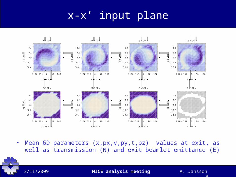
x-x’ input plane

3/11/2009 MICE analysis meeting A. Jansson 6

100 50 0 50 100

0 .4

0 .2

0 .0

0 .2

0 .4

x mm

xprad

xx ,xp

100 50 0 50 100

0 .4

0 .2

0 .0

0 .2

0 .4

x mm xp

rad

pxx ,xp

100 50 0 50 100

0 .4

0 .2

0 .0

0 .2

0 .4

x mm

xprad

yx ,xp

100 50 0 50 100

0 .4

0 .2

0 .0

0 .2

0 .4

x mm

xprad

pyx ,xp

100 50 0 50 100

0 .4

0 .2

0 .0

0 .2

0 .4

x mm

xprad

tx ,xp

100 50 0 50 100

0 .4

0 .2

0 .0

0 .2

0 .4

x mm

xprad

pzx ,xp

100 50 0 50 100

0 .4

0 .2

0 .0

0 .2

0 .4

x mm xp

rad

Nx ,xp

100 50 0 50 100

0 .4

0 .2

0 .0

0 .2

0 .4

x mm

xprad

Nx ,xp

• Mean 6D parameters (x,px,y,py,t,pz) values at exit, as well as transmission (N) and exit beamlet emittance (E)

x’-y’ input plane

3/11/2009 MICE analysis meeting A. Jansson 7

0 .4 0 .20 .0 0 .2 0 .4

0 .4

0 .2

0 .0

0 .2

0 .4

xp rad

yprad

xy , yp

0 .4 0 .2 0 .0 0 .2 0 .4

0 .4

0 .2

0 .0

0 .2

0 .4

xp radyp

rad

pxy , yp

0 .4 0 .2 0 .0 0 .2 0 .4

0 .4

0 .2

0 .0

0 .2

0 .4

xp rad

yprad

yy , yp

0 .4 0 .2 0 .0 0 .2 0 .4

0 .4

0 .2

0 .0

0 .2

0 .4

xp rad

yprad

pyy , yp

0 .4 0 .20 .0 0 .2 0 .4

0 .4

0 .2

0 .0

0 .2

0 .4

xp rad

yprad

ty , yp

0 .4 0 .2 0 .0 0 .2 0 .4

0 .4

0 .2

0 .0

0 .2

0 .4

xp rad

yprad

pzy , yp

0 .4 0 .2 0 .0 0 .2 0 .4

0 .4

0 .2

0 .0

0 .2

0 .4

xp radyp

rad

Ny , yp

0 .4 0 .2 0 .0 0 .2 0 .4

0 .4

0 .2

0 .0

0 .2

0 .4

xp rad

yprad

Ey , yp

• Mean 6D parameters (x,px,y,py,t,pz) values at exit, as well as transmission (N) and exit beamlet emittance (E)

x-y’ input plane

3/11/2009 MICE analysis meeting A. Jansson 8

100 50 0 50 100

0 .4

0 .2

0 .0

0 .2

0 .4

x mm

yprad

xx , yp

100 50 0 50 100

0 .4

0 .2

0 .0

0 .2

0 .4

x mm yp

rad

pxx , yp

100 50 0 50 100

0 .4

0 .2

0 .0

0 .2

0 .4

x mm

yprad

yx , yp

100 50 0 50 100

0 .4

0 .2

0 .0

0 .2

0 .4

x mm

yprad

pyx , yp

100 50 0 50 100

0 .4

0 .2

0 .0

0 .2

0 .4

x mm

yprad

tx , yp

100 50 0 50 100

0 .4

0 .2

0 .0

0 .2

0 .4

x mm

yprad

pzx , yp

100 50 0 50 100

0 .4

0 .2

0 .0

0 .2

0 .4

x mm yp

rad

Nx , yp

100 50 0 50 100

0 .4

0 .2

0 .0

0 .2

0 .4

x mm

yprad

Ex , yp

• Mean 6D parameters (x,px,y,py,t,pz) values at exit, as well as transmission (N) and exit beamlet emittance (E)

Effect of injection position

• Initial dx=0,20,40,60,80,100 mm• At larger amplitudes, exit distribution curls up and spreads out azimuthally

– Distribution is not well described by second moments alone– Large beamlet rms emittance growth at large amplitudes due to nonlinearities

• If beam properly matched, azimuthal spread produces randomization of phases (filamentation), not necessarily emittance (action) increase.

3/11/2009 MICE analysis meeting A. Jansson 9

0 .15 0 .10 0 .05 0 .05 0 .10 0 .15x

0 .15

0 .10

0 .05

0 .05

0 .10

0 .15y

0 .15 0 .10 0 .05 0 .05 0 .10 0 .15x

0 .15

0 .10

0 .05

0 .05

0 .10

0 .15px

0 .15 0 .10 0 .05 0 .05 0 .10 0 .15y

0 .15

0 .10

0 .05

0 .05

0 .10

0 .15py

0 .15 0 .10 0 .05 0 .05 0 .10 0 .15px

0 .15

0 .10

0 .05

0 .05

0 .10

0 .15py

0 .15 0 .10 0 .05 0 .05 0 .10 0 .15x

0 .15

0 .10

0 .05

0 .05

0 .10

0 .15py

0 .15 0 .10 0 .05 0 .05 0 .10 0 .15y

0 .15

0 .10

0 .05

0 .05

0 .10

0 .15px

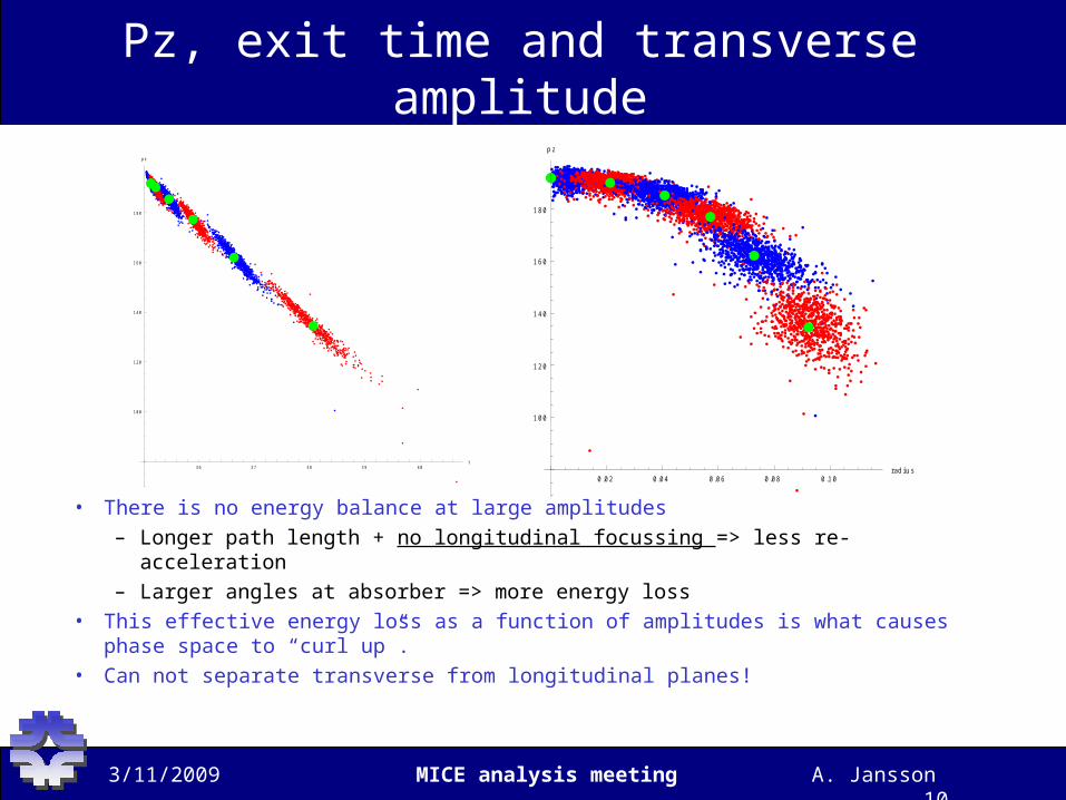
Pz, exit time and transverse amplitude

• There is no energy balance at large amplitudes – Longer path length + no longitudinal focussing => less re-acceleration– Larger angles at absorber => more energy loss

• This effective energy loss as a function of amplitudes is what causes phase space to “curl up”.

• Can not separate transverse from longitudinal planes!

3/11/2009 MICE analysis meeting A. Jansson 10

0 .02 0 .04 0 .06 0 .08 0 .10rad ius

100

120

140

160

180

pz

36 37 38 39 40t

100

120

140

160

180

pz

Pz versus azimuth

• The spread in azimuth is due to the spread in momentum, which in turn comes from energy straggling.– This is a fairly sizeable

effect– May be a way to

measure energy straggling in MICE!

– Requires tight binning in e.g. initial radius coordinate

3/11/2009 MICE analysis meeting A. Jansson 11

3 2 1 1 2 3azimu th

100

120

140

160

180

pz

Effect of injection angle

3/11/2009 MICE analysis meeting A. Jansson 12

0 .15 0 .10 0 .05 0 .05 0 .10 0 .15x

0 .15

0 .10

0 .05

0 .05

0 .10

0 .15y

0 .15 0 .10 0 .05 0 .05 0 .10 0 .15x

0 .15

0 .10

0 .05

0 .05

0 .10

0 .15xp

0 .15 0 .10 0 .05 0 .05 0 .10 0 .15y

0 .15

0 .10

0 .05

0 .05

0 .10

0 .15yp

0 .15 0 .10 0 .05 0 .05 0 .10 0 .15xp

0 .15

0 .10

0 .05

0 .05

0 .10

0 .15yp

0 .15 0 .10 0 .05 0 .05 0 .10 0 .15x

0 .15

0 .10

0 .05

0 .05

0 .10

0 .15yp

0 .15 0 .10 0 .05 0 .05 0 .10 0 .15y

0 .15

0 .10

0 .05

0 .05

0 .10

0 .15xp

36 .0 36 .5t

170

175

180

185

190

195

pz

• Initial dx’=0,100,200,400 mrad.• Same effect as with position offset, although less pronounced (as

momentum correlation is less pronounced).

Conclusions so far

• Energy imbalance for large transverse amplitude particles– This ties transverse and longitudinal planes together and complicates

any “longitudinal slice” analysis– Are these particles “cooled” in any sense? Not clear at this point.

• Normalization of measured deviations by second moments of MC distribution (covariance matrix) does not work for large amplitudes– At least not in cartesian coordinates…

• Perhaps use cylindrical coordinates instead?– Natural because of cylindrical symmetry.– Tight binning may only be required in some coordinates.– E.g. spread in azimuth for large radii may be a way to quantify energy

straggling.– Obviously, more study (and realistic errors) are needed.

3/11/2009 MICE analysis meeting A. Jansson 13