AD-A184 261 COMPUTER-AIDED STRUCTURAL ENGINEERING (CASE) PROJECT 1/1USER'S GUIDE: A THRE..(U) RMY ENGINEER MATERMAYS

EXPERIMENT STATION YICKSBURG MS INFOR. F T TRACY

UNCLAISSIFIED JUN 87 WES/IR/ITL-97-3-i F/O 12/5

mhmmmmsohhhl

U FA bi

EuUS

muk~ TW

"s

IA

Destroy this report when no longer needed. Do not return itto the originator.

The findings in this repor, are not to be construed as an officialDepartment of the Army position unless so designated by other

authorized documents.

This program is furnished by the Government and is accepted and used bythe recipient with the express understanding that the United StatesGovernment makes no warranties, expressed or implied, concerning theaccuracy, completeness, reliability, usability, or suitability for any par-ticular purpose of the information and data contained in this program orfurnished in connection therewith, and the United States shall be under noliability whatsoever to any person by reason of any use made thereof. Theprogram belongs to the Government. Therefore, the recipient furtheragrees not to assert any proprietary rights therein or to represent this

program to anyone as other than a Government program.

The contents of this report are not to be used foradvertising, publication, or promotional purposes.Citation of trade names does not constitute anofficial endorsement or approval of the use of such

commercial products.

_I___

PROGRAM INFORMATION

Description of Program

3DSAD, called X8100 in the Conversationally Oriented Real-Time Program-Generating System (CORPS) Library, is a computer program for a three-dimensional stability analysis/design of hydraulic structures.

Coding and Data Format

3DSAD is written in FORTRAN and is operational on the following systems:

a. US Army Engineer Waterways Experiment Station (WES), Vicksburg,Miss., and Division office Honeywell DPS/8.

b. District office Harris 500.

a. Cybernet Computer Service's CDC CYBER 175.

d. Apollo microcomputer workstation.

Data must be in a prepared data file with line numbers or given interactivelywithout line numbers. Output comes directly back to the terminal or micro-computer monitor. The terminal must be a Tektronix 4014 if graphics displayis wanted.

How to Use 3DSAD

Directions for acessing the program on each of the three systems is providedbelow. It is assumed that the user can sign on the appropriate system beforeattempting to use 3DSAD. In the example initiation of execution commandsbelow, all user responses are underlined, and each should be followed by acarriage return.

Honeywell System

After the user has signed on the system, the system command FORT brings the

user to the level to execute the program. Next, the user issues the runcommand

RUN WESLIB/CORPS/X8100.R

to initiate execution of the program. The program is then run as described inthis user's guide. A data file is typically prepared prior to issuing the runcommand. An example initiation of execution is as follows:

HIS TIMESHARING ON 03/014/81 AT 13.301 CHANNEL 56147USER ID -ROKACASECOL

PASSWORD WHIEERE ARE YOU?*FORT*RUN WESLIB/CORPS/X8 100, R

CYBERNET System

The log-on procedure is followed by a call to the CORPS procedure file

O*DCORPS/UN=CECELB

to access the CORPS library. The file name of the program is used in the

conmmand

BEGIN, ,CORPSX8100

to initiate execution of the program. An example is:

84/12/05. 16.141.00. AC2F5DAEASTERN CYBERNET CENTER SN904 NO!; 1.4/531.669/20ADFAM4ILY: KOEUSER NAM4E- CEROXXPASSWORD-xxxxxxxxTERMINAL: 23, NAMIAFRECOVER/CHARGE: CHARGE ,CEROEGC, CEROXX$CHARGE12.149-07. WARNING (various information messages may appear here)

11/29 FOR IMPORTANT INFO TYPE EXPLAIN,WARNING. (Various information messagesmay appear here.)

OLDCORPS/UN=CECELB/BEGIN, ,CORPS,X8 100

Harris 500 Syste

The log-on procedure is followed by a call to the program executable file,with the user typing the asterisk and file description

'CORPS,X8S100

to intiate execution of the program. An example is:

"1ACOE-ABLESVILLE (H500 V3.1)"ENTER SIGN-ON1234ABC ISTRUCT

"*GOOD MORNING STRUCTURES, IT'S 7 DEC 814 08:33:12AED HARRIS 500 OPERATING HOURS 0700-1800 M-SOCORPSX8100

Apollo Microcomputer Workstation

If 3DSAD is installed under the directory CORPS with the executable file nameX8100, then type

/CORPS/X8100

How to Use CORPS

The CORPS system contains many other useful programs which may be cataloguedfrom CORPS by use of the LIST command. The execute command for CORPS on theHoneywell system is:

RUN WESLIB/CORPS/CORPSRENTER COMMAND (HELP,LIST,BRIEF,MESSAGE,EXECUTE, OR STOP)*?LIST

on the Cybernet system, the commands are:

OLD.CORPS/UN=CECELBBEGIN.,CORPSENTER COMMAND (HELP,LIST,BRIEF,MESSAGE,EXECUTE, OR STOP)MLIST

on the Harris system, the commands are:

*CORPSARE YOU USING A PRINTER TERMINAL OR CRT?ENTER P OR CPCORPS SYSTEM COMMANDS:BRIEF - LIST EXPLANATION OF A PROGRAM.EXECUTE - RUN A CORPS PROGRAM.LIST - LIST THE AVAILABLE CORPS PROGRAMS.STOP - EXIT FROM CORPS SYSTEM MACRO.HELP - HELP AND EXPLANATION OF CORPS

SYSTEM AND THE RUNNING OF ITS MACRO.

NOTE: COMMANDS MAY BE ABBREVIATED TO THEFIRST LETTER OF THE COMMAND.

ENTER COMMAND (BRIEF,EXECUTE,LIST,HELP,STOP):LIST

This capability is not yet implemented on the Apollo.

- ~9 -

ELECTRONIC COMPUTER PROGRAM ABSTRACT

TITLE OF PROGRAM A Three-Dimensional Stability Analysis/ PROGRAM NO.

Dagion Program (IDSAD) (X8100) I 713F3-RO08PREPARING AGENCY US Army Engineer Waterways Experiment Station, Information

ghngnl oav bgratory - PO Box 631. Vicksbur. MS 39180-0631AUTHORIS) -- DATE PROGRAM COMPLETED "STATUS, OF PROGRAM

PHASE STAGE

Fred T. Traov September 1986 OP

A. PURPOSE OF PROGRAMi

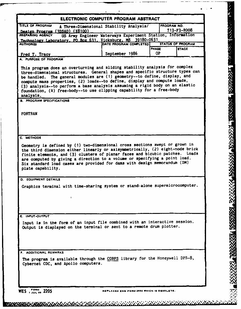
This program does an overturning and sliding stability analysis for complex

three-dimensional structures. General shapes and specific structure types can

be handled. The general modules are (1) geometry--to define, display, and

compute mass properties, (2) loads--to define, display and compute loads,

(3) analysis--to perform a base analysis assuming a rigid body on an elastic

foundation, (4) free-body--to use clipping capability for a free-bodyanalysis.8. PROGRAM SPECIFICATIONS

FORTRAN

C. METHODS

Geometry is defined by (1) two-dimensional cross sections swept or grown in

the third dimension either linearly or axisymmetrically, (2) eight-node brick

finite elements, and (3) clusters of planar faces and bicubic patches. Loads

are computed by giving a direction to a volume or specifying a point load.

Six standard load cases are provided for dams with design memorandum (DM)plate capability.

0. EQUIPMENT DETAILS

Graphics terminal with time-sharing system or stand-alone supermicrocomputer.

E. INPUT-OUTPUT

Input is in the form of an input file combined with an interactive session.

Output is displayed on the terminal or sent to a remote drum plotter.

F. ADDITIONAL REMARKS

The program is available through the CORPS library for the Honeywell DPS-8,Cybernet CDC, and Apollo computers.

ES, 2205 ,PLACI ,. FO 20 0... WHISCH 1. .8OLCET.nrzm .1-%

"

. . . .oC'P'*

REPORT DOCUMENTATION PAGE

as REPORT SECURITY CLASSIFICATION lb RESTRICTIVE MARKINGS

2.. S6CUIRITY CLaSSIFICATION AUTHOR0ITY 3 DISTRIBUTION I AVAILAILITY OF REPORT

Uab cLssifiedINO*WNON SOOL Approved for public release;2b. ICLSSW"ON 00110WA&WIHIOL11distribution unlimited

& Pt"ONMA4 ORANUZTIO REPORT NUM04*(S) S. MONITORING ORGANIZATION REPORT NUMBER(S)

Instruction Report ITL-87-3a~g p OF too nauM a FICE SYMBOL 7a. NAME OF MONITOING ORGANIZTON

USAEIIES InformationOf011*1:061)Technoloa Laboratorv WESIM-RS _____________________

Bi AIORIESS (COX. stft. ad ZC0111) 7b. ADDRESS (ft, Stag.. and ZIP Code)

PO Box 631

B.NAME OF FUNOINGISPONISORING all.OFFCE SYMBOL 9. PROCUREMENT INSTRUMENT IDENTIFICATION NUMBERORGANIZATION OfV apc.M0*8111j

US91r&= Corns of Enzineer3 ______________________

Bct ADDRESS (aRp, Stat. Will ZIP Code) 10. SOURCE OF FUNDING NUMBERSPROGRAM PROJECT TASK WORK UNIT

Washington, DC 2031)4-1000 ELEMENT No. No. No. ACCESSION NO.

itI TITLE onui Securiy CAafas.ion

User's Guide: A Three-Dimensional Stability Analysis/Design Program (3DSAD) Report 1

Reviion *__Qer1 Geometry Module12 PERSONAL AUTHO(S)

3.TrayE OFre REOT.bTM OEE 14. DATE OF REPORT (Year, Moanth. Day) S. PAGE COuNT

Rprt1oa series PROMoTO 86 June 1987 5916 SUPPLEMENTARY NOTATION

This report was prepared under the Computer-Aided Structural Engineering (CASE) Project. A

lis of published CASE reports is printed on the inside of the back cover17 COSATI CODIES 1B SUBJECT TERMS (Continue, an reverse of necessary and idlentfyv by block number)

FIELD GROUP SUB-GROUPSee reverse

'9 ABSTRACT (Cont Vme, on reVeis Of neceuaip and identilify by block number)

This module of the three~dimensional (3-D) stability analysis/design program (3DSAD)

enables the engineer to describe the geometry of the 3-D structure, to interactively plot

the desired structure, and then to obtain volume, weight, and centroidipformat ion for the

structure. The general ways in which geometry is deqoribed are (a) two dimensional cross

sections extended in the third dimension, (b) eight-node brick elements, and (c) clusters

of planar polygonal and bicubic patches. Curved segments can be circular, elliptical, or

quadratic when using blocks and cubic when using patches. Objects can be copied, trans- .m

lated, rotated, or reflected about an axis as well. An arbitrary clipping plane can also be

passed through the geometry. /,-iP

20 OISTRfSUTIONIAVAILAIILITY OF ABSTRACT 21 ABSTRACT SECURITY CLASSIFICATION

ONCLASSIFIEDIJNLIMITE0DC SAME AS RPT C3DTIC USERS UnclassifiedL22. N=AMEOF RESPONSIBLE INDI4VIDUAL 22b TELEPHONE (Include Area Code) 22C. OFFICE SYMBOL

00 FRM 473B4MA B3PR~~tmomayeu~duntlexaused.SECURITY CLASSIFICATION OF THIS PAGEAll other editions are obsolete.

Unclassified

UnclassifiedaaMm OLAimMAON~~ OF T"W PA44

18. SUBJECT TERMS (Continued).

SCoputerfided design, -_ GeometryComputer-Aided Structural Engineering Project--3 Structural analysisComputer programs Structural design

L:.

UnclassifiedSIRCUITY CLAUIsIICA1ION OF THIS PAGE

-. ~ Up * •

PREFACE

This report documents the General Geometry Module of the three-

dimensional stability analysis/design (3DSAD) program. The module was de-

veloped and this report was written at the US Army Engineer Waterways Experi-

ment Station (WES), Vicksburg, Miss., in the Information Technology Laboratory

(ITL), formerly the Automation Technology Center, by Mr. Fred T. Tracy. The

work was sponsored through funds provided WES by the Engineering and Con-

struction Directorate, Office, Chief of Engineers (OCE), US Army, under the

Computer-Aided Structural Engineering (CASE) Project.

Specifications for the program were provided by the members of the CASE

Task Group on 3-D Stability. The members of the task group during the initial

period of development were as follows:

Mr. Charles Kling, Mobile District (Chairman)Mr. Robert Haavisto, Sacramento DistrictMr. John Hoffmeister, Nashville DistrictMr. Gerrett Johnson, Seattle DistrictMr. Thomas Mudd, St. Louis DistrictMr. William Holtham, New England Division

Members of the task group during the latest development were:

Mr. Kling (Chairman)Mr. Lavane Dempsey, St. Paul DistrictMr. Jack Duckworth, Federal Energy Regulatory

Commission (FERC)Mr. Steve Freitas, Sacramento DistrictMr. HolthamMr. JohnsonMr. Tom Leicht, St. Louis District

Mr. Donald R. Dressler, Structures Branch, Engineering and Construc-

tion Directorate, was the OCE point of contact. The work was done under the

supervision of Dr. N. Radhakrishnan, Acting Chief (AC), ITL, and Mr. Paul K.

Senter, AC, Information Research Division, ITL. Mr. Dressler and

Dr. Radhakrishnan also contributed in the definition of general concepts for

the development of 3DSAD. The report was prepared for publication by

Ms. Gilda Miller, Editor, Information Products Division, ITL, WES. 0

COL Allen F. Grum, USA, was the previous Director of WES. COL Dwayne G.

Lee, CE, is the present Commander and Director. Dr. Robert W. Whalin is

Technical Director.

istd,

CONTENTS

Page

PREFACE................................................................ 1

PART I: OVERVIEW OF THE THREE-DIMENSIONAL STABILITY PROGRAM ............ 3

The General Geometry Module ........................................ 4Coordinate System................................................ 5Data Types........................................................ 5

PART II: RUNNING THE PROGRAM.......................................... 10

Commands......................................................... 10Practical Applications........................................... 33

REFERENCES............................................................. 34

PLATES 1-3

APPENDIX A: THEORY AND PROCEDURE FOR COMPUTING MASS PROPERTIES .......... Al

Introduction..................................................... AlModeling Technique............................................... AlMass Properties--BLOCK........................................... AlMass Properties--FACES........................................... A

2

USERS GUIDE: A THREE-DIMENSIONAL STABILITY

ANALYSIS/DESIGN PROGRAM (3DSAD)

REVISION 1: GENERAL GEOMETRY MODULE

PART I: OVERVIEW OF THE THREE-DIMENSIONALSTABILITY PROGRAM

1. The objective of the Computer-Aided Structural Engineering (CASE)

Task Group on Three-Dimensional (3-D) Stability Analysis is to develop com-

puter programs to aid design engineers perform stability computations for

general 3-D structures (Tracy 1980; Tracy and Kling 1982; and Tracy, Kling,

and Holtham 1983). To enable this, a computer program called 3DSAD (3-D

stability analysis/design) has been developed in a modular fashion. Cur-

rently, 3DSAD has four "general" modules:

a. General Geometry Module.

(1) Defines geometry based on two-dimensional (2-D) crosssections extended into the third dimension, eight-nodebrick elements, or clusters of planar polygonal or bicubicpatches.

(2) Performs centroid, volume, and weight computations ondescribed geometry.

(3) Employs interactive graphics extensively.

b. General Loads Module. This module uses "pressure volumes" andpoint loads to compute forces and moments for a general 3-Dstructure. It will eventually compute loads based on input ofgeometry, water levels, and soil strata descriptions only withthe pressure volumes (or equivalent surface integration)generated automatically.

c. General Analysis Module. This module performs overturning,bearing, and sliding computations.

d. Free-Body Module. This module "clips" the structure and loadsby an arbitrary plane to produce a "free-body" so thatcomputations can be performed on the new part.

The engineer performing an analysis of any 3-D structure can interact directly

with these modules.

2. In addition to the general capabilities that are useful for any

3-D structures, 3DSAD also provides for simplified geometry and load imput

along with criteria check modules for certain structures. This latter capa-

bility will permit interactive design of these structures. Examples of spe-

cific structures for which modules can be developed are dams, locks, walls,

powerhouses, and pumping stations.

3

3. A specific structure input module requires less data than that for

a general structure. Modules of this type will interact with the General Ge-

ometry Module and the General Loads Module to define the geometry and loads

internally in the program. After analysis, a specific structure criteria

check module will verify pertinent values, change dimensions (if necessary),

and cycle through the computations. A general schematic of the 3DSAD program

is shown in Figure 1.

SSPECIFIC STRUCTURE

GEOMETRY LOAS NALYSISMODULE MODULE MODULE

ITERATION SPECIFIC STRUCTURE

CRITERIA CHECK MODULES

SECIFIC STRUCTURE]

OUTPUT MODULES

Figure 1. General schematic of 3DSAD

4. The 3DSAD program has been developed in phases. During the first

phase, the first three general modules were developed. This approach enabled

the stability analysis of any 3-D structure although the imput is more com-

plicated than need be for certain structures. In the subsequent phases, the

special input and criteria check modules were developed for several spe-

cific structures. Also, new general modules such as the Free-Body Module

have been added.

The General Geometry Module

5. This report is an updated user's guide for the General Geometry

Module (the original is IR K-80-4). As stated in paragraph la this module

enables the engineer to describe the geometry of a 3-D structure, to inter-

actively plot the described structure, and then to obtain volume, weight, and

4

- N JA 1.~ '1 , * l, 1 1

centroid information for the structure. In the stand-alone mode of operation

for a general structure, the user first creates a data file and stores it in a

permanent disc file. He then uses the graphics to verify the data. When

satisfied, the user types

VOLUME

to obtain the resultant volume, weight, and centroid of the sturcture. Appendix

A contains a mathematical presentation on how the mass properties are computed.

Coordinate System

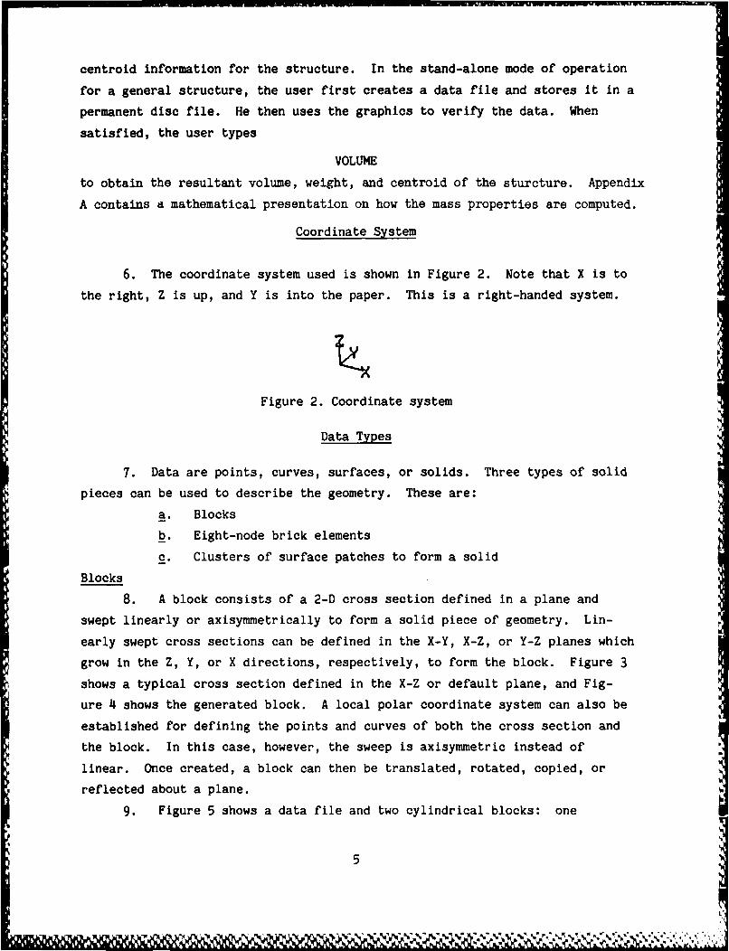
6. The coordinate system used is shown in Figure 2. Note that X is to

the right, Z is up, and Y is into the paper. This is a right-handed system.

Figure 2. Coordinate system

Data Types

7. Data are points, curves, surfaces, or solids. Three types of solid

pieces can be used to describe the geometry. These are:

a. Blocks

b. Eight-node brick elements

c. Clusters of surface patches to form a solid

Blocks

8. A block consists of a 2-D cross section defined in a plane and

swept linearly or axisymmetrically to form a solid piece of geometry. Lin-

early swept cross sections can be defined in the X-Y, X-Z, or Y-Z planes which

grow in the Z, Y, or X directions, respectively, to form the block. Figure 3

shows a typical cross section defined in the X-Z or default plane, and Fig-

ure 4 shows the generated block. A local polar coordinate system can also be

established for defining the points and curves of both the cross section and

the block. In this case, however, the sweep is axisymmetric instead of

linear. Once created, a block can then be translated, rotated, copied, or

reflected about a plane.

9. Figure 5 shows a data file and two cylindrical blocks: one

5

Figure 3. 2-D cross Figure 4. Generated blocksection

10 XZ20 POINTS 430 1 -5 0 040 2 0 0 550 3 5 0 060 4 0 0 -570 CIRCLE 1 2 580 CIRCLE 2 3 590 CIRCLE 3 4 5100 CIRCLE 4 1 S110 BLOCK BLI .15 40120 1 1130 4 1 2 3 4140 XY150 POINTS 4160 5 -5 20 5170 6 0 15 5180 7 5 20 5190 8 0 25 5200 CIRCLE 5 6 5210 CIRCLE 6 7 5220 CIRCLE 7 8 5230 CIRCLE 8 5 5240 BLOCK BL2 .IS 4C250 1 1260 4 5 6 7 8

Figure 5. Two cylinders

6

generated from an X-Z cross section and the other from an X-Y cross section.

Note that in the data file "XZ" indicated that the data refer to the X-Z plane

and that "XY" is used when the switch is made to referring to the X-Y plane.

Also, points are first defined, then any curves, and finally the block it-

self. The cross sections are specified by giving the point numbers defining

the section in a counterclockwise positive manner according to the right-hand

screw rule. For example, a cross section defined in the X-Z plane will grow

into a block alone the Y axis. Thus, if the user is looking in the negative

Y direction, he must give the connectivity in a counterclockwise order to get

a positive volume and weight. In like manner, a cross section defined in the

X-Y plane grows in the Z direction and will have its connectivity specified in

a counterclockwise manner by a user looking in the negative Z direction to ob-

tain a positive volume. If the connectivity is reversed, the volume will be

negative.

10. The line segments describing the cross section can be straight,

circular, quadratic, or elliptical. Further, the section can grow smaller or

larger as it is extended in the perpendicular direction. Any number of holes

(for culverts, etc.) can be defined in the cross section as well.

Brick

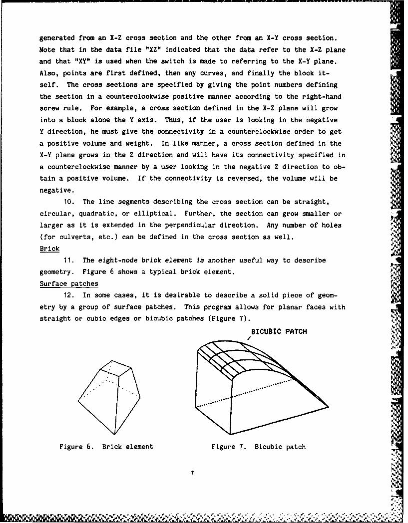
11. The eight-node brick element Is another useful way to describe

geometry. Figure 6 shows a typical brick element.

Surface patches

12. In some cases, it is desirable to describe a solid piece of geom-

etry by a group of surface patches. This program allows for planar faces with

straight or cubic edges or bicubic patches (Figure 7).

BICUBIC PATCH

Figure 6. Brick element Figure 7. Bicubic patch

7

STRUCTURE TYPE OR GENERAL MODULE ?

13. If the user types a "?", the following message will appear:

A THREE-DIMENSIONAL STABILITY ANALYSIS/DESIGN PROGRAM

(3DSAD)

A PRODUCT OF

Computer Aided Structural Engineering

(CASE)

PROGRAM NO. 713-F3-RO-008

Computer Aided Design (CAD) OF STRUCTURAL STABILITY

() (0 (0 () (0 (0

ENTER ?, HELD, OR WHAT TO GET VALID RESPONSES.

ENTER STOP, END, QUIT, OR DONE TO TERMINATE PROGRAM.

STRUCTURE TYPE OR GENERAL MODULE ?

The user then gives

GEOM

for the General Geometry Module.

14. The next question the program asks is

RESTART FILE NAME OR CR?

when "CR" stands for carriage return. The restart file saves all data per-

taining to building structure. These include any data input from another data

file. The user gives a carriage return if he does not want a restart file.

15. The next question is

OUTPUT FILE NAME OR CR?

In this file is placed the resulting weight and centroid of the structure in

the form of a point load; for example,

2 PTLD WT 17.584 20.000 1.004 0. 0. -8,067.939

The file consists of one line with line number 2, X centroid of 17.584, Y

Centroid of 20.000, Z Centroid of 11.004, and weight of 8,067.939. A

8

N~ , . .,

carriage return is given if an output file is not wanted. The file is written

when the RETURN command is given.

16. The third question is

COMMAND?

The commands are discussed in detail in the next section.

9

PART II: RUNNING THE PROGRAM

Commands

17. The program uses commands (PLOT, ROTP, etc.) to both build and plot

the data. The commands are:

a. Data building:

XY XZ YZ RTZPOINT

CIRCLE ELLIPSEQUADRATICBLOCK FACE

BR8TRANSLATE

ROTD COPY REFLECT

b. Utility:

INPUT VOLUMEEND GO RETURN

CLIP CLEAR

c. Plotting:

PLOT WINDOW ZOOMROTP ISOMETRICLABEL NOLABEL

DASH HIDE SOLIDERASE INITIALIZE

This list is obtained by typing "?" at the command level. Only the minimum

number of letters of a command need to be given. The user can, however, type

the entire word if he prefers. Commands and their accompanying data can be

put into a data file or typed interactively while running the program. The

basic command sequence is:

INPUT FILENAME Read data from file FILENAME

PLOT Plot data

VOLUME Compute and print volume

END End

18. Each command will now be described in detail. In giving the format

for the commands, actual letters to be typed will be enclosed in the quotes to

distinguish them from variable names. The quotes do not have to be typed when

the user issues the command. The required letters are shown in all capitals;

10

the optional letters are shown in lower-case letters."XY"

19. The format for this command is

"iXy"

This command turns on the flag that states that all "Circle" and "ELlipse"

commands define circular and elliptical arcs in the X-Y plane, and all

"BLocks" commands start with cross sections in the X-Y plane and grow in the

Z direction (Figure 5 and the associated data file). This condition is held

until an XZ, YZ, or "RTZ" command is encountered.

20. The format for this command is

This command is like XY except that circular and elliptical arcs are defined

in the X-Z plane, and blocks start with cross sections in the X-Z plane and

grow in the Y direction. XZ is assumed until an XY, YZ, or RTZ command is

encountered. XZ is the default condition.

21. The format for this command is

This command is like XY and XZ except that circular and elliptical arcs are

defined in the Y-Z plane, and blocks start with cross sections in the Y-Z

plane and grow in the X direction. YZ remains in effect until an XY, XZ, or

RTZ command is encountered."IRTZ"

22. This command establishes a local polar coordinate system (Radius-

Theta-Z) in space. The Z axis is established by two specified points (Xl, Y1,

Z1) and (XZ, Y2, Z2), and (Xl, Y1, ZI) is the new origin. The format of the

command is

"RTZ" X1 Y1 ZI X2 Y2 Z2

Theta is zero in the R-Theta plane where the new local Z axis strikes the

R-Theta plane when projected vertically. If the new local Z axis is vertical,

theta is zero along the line parallel to the X axis and passing through

(I, YI, Zi). All coordinates of points are specified in this system until

another is specified. Also, the BLOCK command now expects an angle in degrees

to produce a volume swept by a rotation rather than a translation. The cross

section for a block can have curved or straight line segments as before, but

the points defining the cross section must all have the same THETA value.

Figure 8 shows a sample data file with its plot. RTZ is in effect until the

X¥, XZ, or YZ command is given.

10 RTZ 6. 5. 0. 6. 5. 1.20 POINTS 430 1 10. 30. 2.40 2 10. 30. 10.50 3 15. 30. 10.60 4 15. 30. 2.70 BLOCK BLI .1 90.80 1. 1.90 4 1 2 3 4

Figure 8. RTZ example

"POints"

23. The user first defines points using the POINTS command. The format

is

"POints" NPT

where NPT is the number of points. After this line, an identification number

and (X, Y, Z) coordinates for each point are given.

24. Interactive mode. An example of the POINTS command when made in-

teractively on the CDC system is shown:

12

CINNABD ?POINTS 14N, X, Y, Z1 0 0 5652 44 0 5653 44 0 577.4 40 0 5775 40 0 5976 22 0 6177 22 0 6338 4 0 6339 4 0 57710 0 0 57711 9 0 58512 9 0 59513 19 0 59514 19 0 585COMMAND ?

When RTZ has been specified, X, Y, and Z become R, THETA, and Z in the local

polar coordinate system.

25. Data file mode. The same data are put in a file as shown below:

10 POINTS 1420 1 0 0 56530 2 44 0 56540 3 44 0 57750 4 40 0 57760 5 40 0 57770 6 22 0 61780 7 22 0 63390 8 4 0 633100 9 4 0 577110 10 0 0 577120 11 9 0 585130 12 9 0 595140 13 19 0 595150 14 19 0 585

"Circle"

26. After the user has defined points to work with, he must then define

any curved line segments. That is, line segments between points are assumed

straight unless otherwise specified. The possible ways of using Circle

command are

"Circle" N1 N2 R"Circle" Ni N2 R "Left""Circle" NI N2 R "Right"

NI and N2 are two point numbers connected by a circular arc of radius R.

13

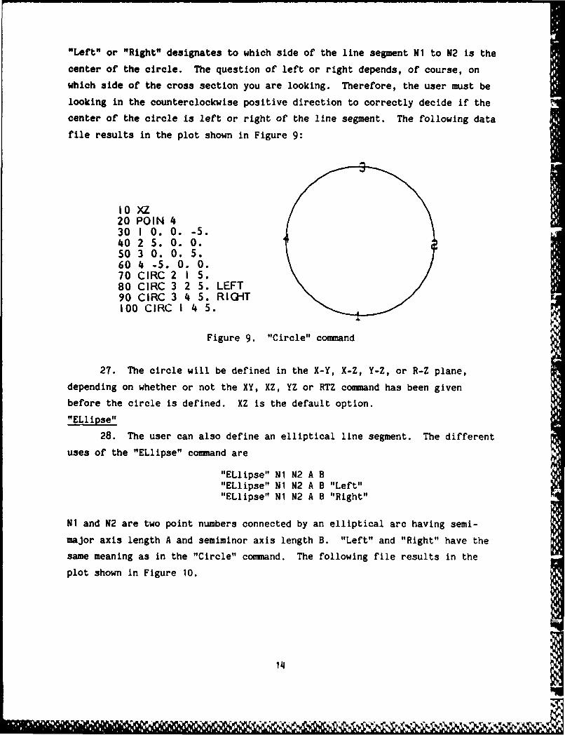
"Left" or "Right" designates to which side of the line segment Ni to N2 is the

center of the circle. The question of left or right depends, of course, on

which side of the cross section you are looking. Therefore, the user must be

looking in the counterclockwise positive direction to correctly decide if the

center of the circle is left or right of the line segment. The following data

file results in the plot shown in Figure 9:

10 XZ20 POIN 430 1 0. 0. -5.40 2 5. 0. 0.50 3 0. 0. 5.60 4 -5. 0. 0.70 CIRC 2 1 5.80 CIRC 3 2 5. LEFT90 CIRC 3 4 5. RIG-IT100 CIRC I 4 5.

Figure 9. "Circle" command

27. The circle will be defined in the X-Y, X-Z, Y-Z, or R-Z plane,

depending on whether or not the XY, XZ, YZ or RTZ command has been given

before the circle is defined. XZ is the default option.

"ELlipse"

28. The user can also define an elliptical line segment. The different

uses of the "ELlipse" command are

"ELlipse" Ni N2 A B"ELlipse" Ni N2 A B "Left""ELlipse" Ni N2 A B "Right"

Ni and N2 are two point numbers connected by an elliptical arc having semi-

major axis length A and semiminor axis length B. "Left" and "Right" have the

same meaning as in the "Circle" command. The following file results in the

plot shown in Figure 10.

- r - 14

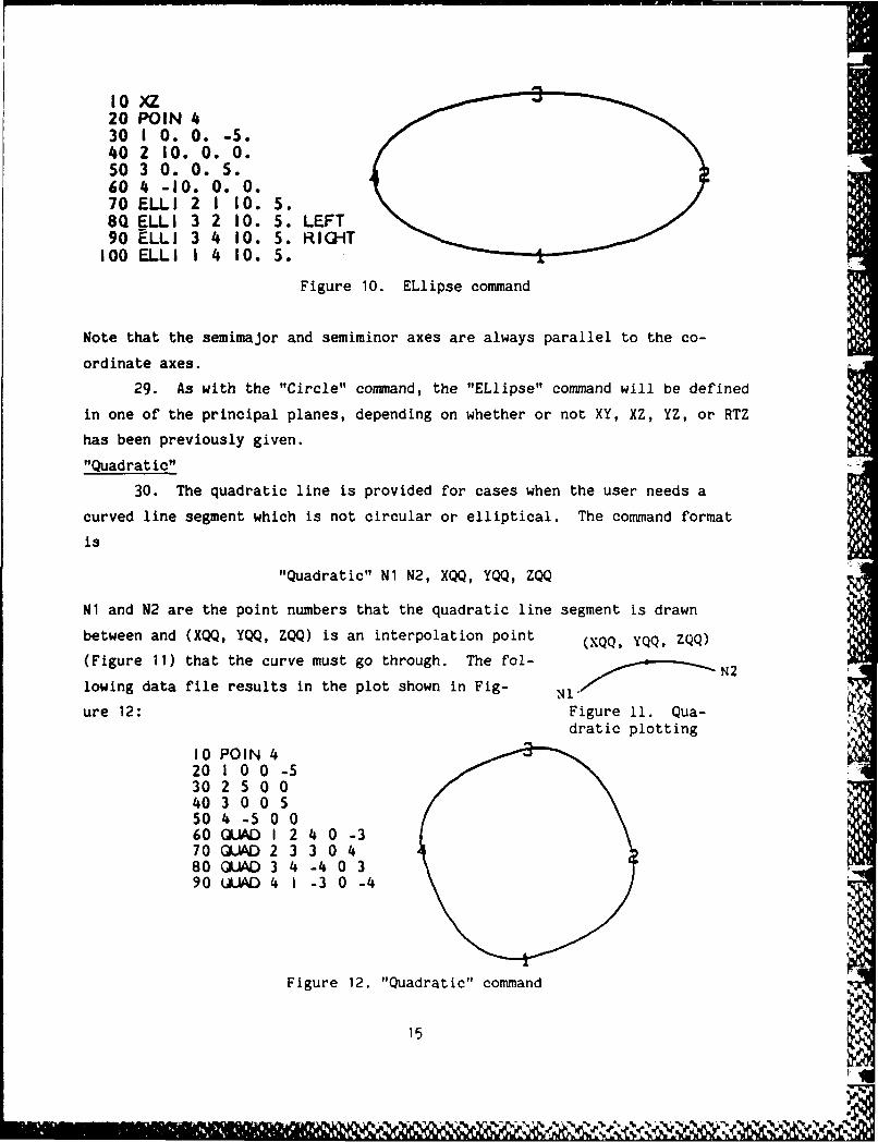
10 )a20 POIN 430 I 0. 0. -5.40 2 10. 0. 0.50 3 0. 0. 5.60 4 -10. 0. 0.70 ELI 2 1 10. 5.8Q ELLI 3 2 10. 5. LEFT90 .LLI 3 4 10. 5. RIGIT100 ELLI I 4 10. 5.

Figure 10. ELlipse command

Note that the semimajor and semiminor axes are always parallel to the co-

ordinate axes.

29. As with the "Circle" command, the "ELlipse" command will be defined

in one of the principal planes, depending on whether or not XY, XZ, YZ, or RTZ

has been previously given.

"Quadratic"

30. The quadratic line is provided for cases when the user needs a

curved line segment which is not circular or elliptical. The command format

is

"Quadratic" N1 N2, XQQ, YQQ, ZQQ

Ni and N2 are the point numbers that the quadratic line segment is drawn

between and (XQQ, YQQ, ZQQ) is an interpolation point (XQQ, YQQ, ZQQ)

(Figure 11) that the curve must go through. The fol- N2

lowing data file results in the plot shown in Fig- N o

ure 12: Figure 11. Qua-

dratic plotting

10 POIN 4

20 i 0 0 -530250040 3 0 0 550 4 -5 0 060 GU.AD I 2 4 0 -370 QUAD 2 3 3 0 480 GLAD 3 4 -4 0 390 ULAD 4 i -3 0 -4

Figure 12. "Quadratic" command

15

when RTZ has been specified, XQQ, YQQ, and ZQQ become RQQ, TQQ, and ZQQ in the

local polar coordinate system.

"BLock"

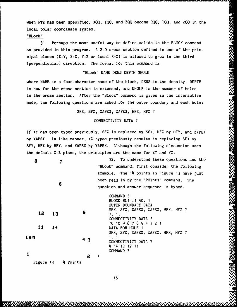
31. Perhaps the most useful way to define solids is the BLOCK command

as provided in this program. A 2-D cross section defined in one of the prin-

cipal planes (X-Y, X-Z, Y-Z or local R-Z) is allowed to grow in the third

(perpendicular) direction. The format for this command is

"BLock" NAME DENS DEPTH NHOLE

where NAME is a four-character name of the block, DENS is the density, DEPTH

is how far the cross section is extended, and NHOLE is the number of holes

in the cross section. After the "BLock" command is given in the interactive

mode, the following questions are asked for the outer boundary and each hole:

SFX, SFZ, XAPEX, ZAPEX, HFX, HFZ ?

CONNECTIVITY DATA ?

If XY has been typed previously, SFZ is replaced by SFY, HFZ by HFY, and ZAPEX

by YAPEX. In like manner, YZ typed previously results in replacing SFX by

SFY, HFX by HFY, and XAPEX by YAPEX. Although the following discussion uses

the default X-Z plane, the principles are the same for XY and YZ.

8 7 32. To understand these questions and the

"BLock" command, first consider the following

example. The 14 points in Figure 13 have just

been read in by the "POints" command. The

question and answer sequence is typed.

COMMAND ?BLOCK BLI .1 50. 1OUTER BOUNDARY DATASFX, SFZ, XAPEX, ZAPEX, HFX, HFZ ?

12 13 1. 1.CONNECTIVITY DATA ?1010987654321

11 14 DATA FOR HOLE 1SFX, SFZ, XAPEX, ZAPEX, HFX, HFZ ?

CONNECTIVITY DATA ?4 14 13 12 11COMMAND ?

Figure 13. 14 Points

16

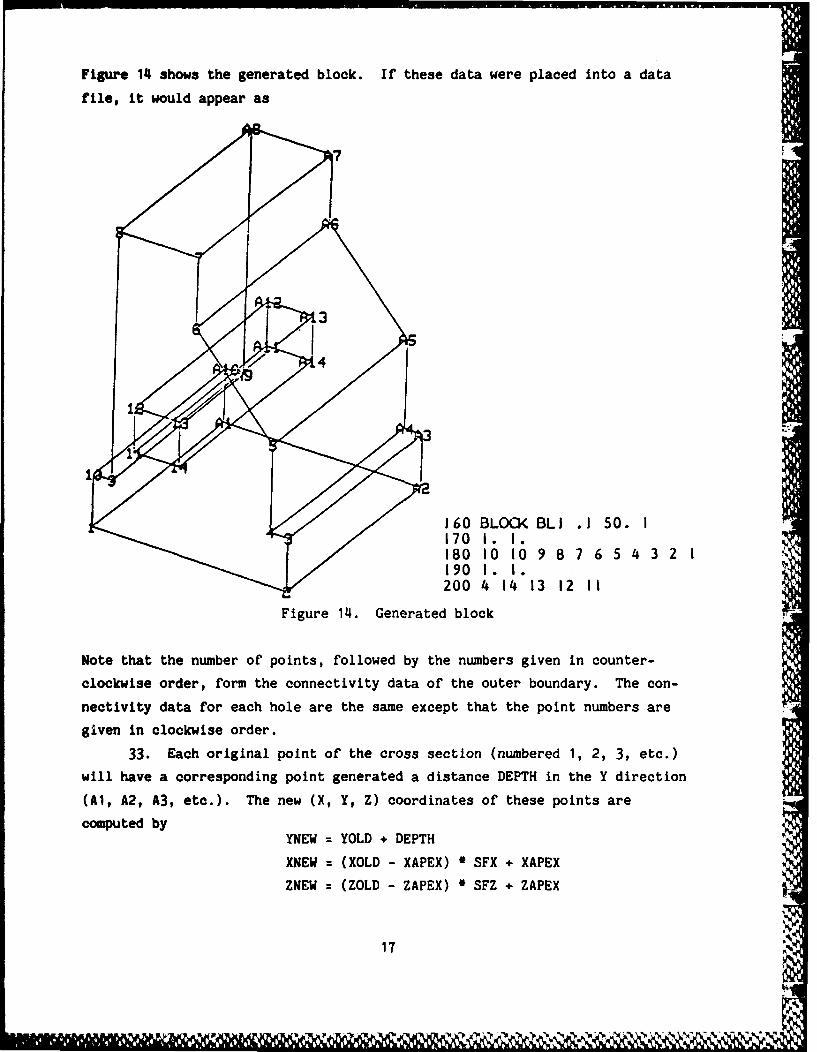
Figure 14 shows the generated block. If these data were placed into a data

file, it would appear as

• 4-

160 BLOCK BLI .1 50. I170 1. I.180 10 10 9 8 7 6 5 4 3 2 i190 I. I.200 4 14 13 12 II

Figure 14. Generated block

Note that the number of points, followed by the numbers given in counter-

clockwise order, form the connectivity data of the outer boundary. The con-

nectivity data for each hole are the same except that the point numbers are

given in clockwise order.

33. Each original point of the cross section (numbered 1, 2, 3, etc.)

will have a corresponding point generated a distance DEPTH in the Y direction

(Al, A2, A3, etc.). The new (X, Y, Z) coordinates of these points are

computed byYNEW = YOLD + DEPTH

XNEW = (XOLD - XAPEX) * SFX + XAPEX

ZNEW = (ZOLD - ZAPEX) * SFZ + ZAPEX

17

11~~~1 li S ' ..

Note that if SFX and SFZ are equal to one, then

XNEW = XOLD

ZNEW = ZOLD

These are independent of the apex (XAPEX, ZAPEX). This allows XAPEX and ZAPEX

in the data for Figure 14 to default to zero.

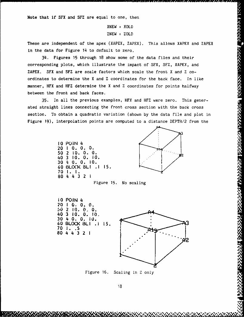
34. Figures 15 through 18 show some of the data files and their

corresponding plots, which illustrate the impact of SFX, SFZ, XAPEX, and

ZAPEX. SFX and SFZ are scale factors which scale the front X and Z co-

ordinates to determine the X and Z coordinates for the back face. In like

manner, HFX and HFZ determine the X and Z coordinates for points halfway

between the front and back faces.

35. In all the previous examples, HFX and HFZ were zero. This gener-

ated straight lines connecting the front cross section with the back cross

section. To obtain a quadratic variation (shown by the data file and plot in

Figure 19), interpolation points are computed to a distance DEPTH/2 from the

10 POIN 420 1 0. 0. 0.50 2 10. 0. 0.40 3 10. 0. 10.30 4 0. 0. 10.60 BLOC< BLI .1 15.70 I. I.80 4 4 3 2 1

Figure 15. No scaling

10 POIN 420 1 0. 0. 0.!Q 2 10. 0. 0.40 3 10'. 0. 10.30 4 0. 0. 10.60 BLOCK BLI .1 15.70 I. .580 4 4 3 2 I

Figure 16. Scaling in Z only

18

10 POIN 4Figure 17. Scaling in X 20 1 0. 0. 0.3and Z with nonzero apex, 50 2 10. 0. 0.

240 3 10. 0. 10.straight line segments 30 4 0. 0. 10.

60 BLOG( BLI .1 15.70 .5 .5 5. 5.80 4 4 3 2 1

10 POIN 420 1 0. 0. -5.30 2 5. 0. 0.40 3 0. 0. 5.50 4 -5. 0. 0.60 CIRC 2 1 5.70 CIRC 3 2 5.80 CIRC 4 3 5.90 CIRC 1 4 5.100 BLOG< BLI .1 I5.110 .5 S5 0. 0.120 4 4 3 2 1

Figure 18. Scaling in X and Z with non-zero apex, circular line segments

JO POIN 420 1 0. 0. 0.50 2 10. 0. 0.bO 3 10. 0. 10.30 4 0. 0. 10.60 BLOO( BLI .1 15.70 .3 .3 5. 5. .8 .880 44 32 1

Figure 19. Quadratic variation

19

front face for all the connecting line segments. The (X, Y, Z) coordinates of

each interpolation point are computed by

YINT = YOLD + DEPTH * .5

XINT = (XOLD - XAPEX) * HFX + XAPEX

ZINT = (ZOLD - ZAPEX) * HFZ + ZAPEX

"FAce"

36. The "I'Ace" command is used to define a solid object by giving a

boundary representation of its faces. Faces can consist of

a. Planar faces with straight or cubic sides.

b. Bicubic patches defined by 16 (X, Y, Z) points.

The format for this command is as follows:

"FAce" NAME DENS NFACE"FAce" DIR NAME DENS NFACE

"P" NPT PT1 PT2 . . . PTN(WHERE N = NPT) (FOR PLANAR FACE)

orNPT PT1 PT2 . . PTN(WHERE N = NPT) (FOR PLANAR FACE)

or"C" PT1 PT2 . . . PT16 (FOR BICUBIC PATCH)

NOTE -- THE ABOVE INDENTED LINES ARE REPEATEDFOR EACH REMAINING FACE.

where NAME is a four character name, DENS is the density of the object being

defined, and NFACE is the number of faces to be defined. Notice that next

comes the connectivity of each face with a P to designate a planar face, and a

C to designate a bicubic patch. If no letter is specified, P is the assumed

default. The connectivity of a planar face consists of the number of points

of the polygon followed by the point numbers. The order of the points must be

counterclockwise if the outward normal to the face points out of the picture

(-Y direction). The connectivity of a bicubic patch consists of the 16 points

given a row at a time from left to right and from bottom to top (assuming the

outward normal of the patch is pointing toward the observer). Figure 20 shows 'V

an eighth of a sphere defined using the 'FAce' definition capability. The

sample problem therefore consists of one bicubic patch and three planar faces.

As before, the faces must be numbered so that a right-hand screw advances

toward the outward normal (holes can be produced by reversing this process) .4

when turned in the direction of the numbering. k37. Bicubic Patch. This patch was chosen not only for its ability to

20

--- - U --

10 RTZ 50. 50. 50. 50. 50. 51.20 POIN 1430 I 10. 0. 0.40 2 10. 30. 0.50 3 10. 60. 0.60 4 10. 90. 0.70 5 8.66 0. 5.80 6 8.66 30. 5.90 7 8.66 60. 5.100 8 8.66 90. 5.110 9 5. 0. 8.66120 10 5. 30. 8.66130 i 5. 60. 8.66140 12 5. 90. 8.66150 13 0. 0. 10.160 14 0. 0. 0.170 FACE SPHI .1 4180 C I 2 3 4 5 6 7 8 9 10 II 12 13 13 13 13190 P 3 14 4 I200 P 3 14.1 13210 P 3 14 13 4

Figure 20. One-eighth of a sphere

model general shapes, but also for its accuracy when modeling conic sections.

Note that it has 14 points given by rows as shown. Four points can also

coincide (as was needed in the sample) to form a triangular shaped patch. If

the patch is being used to model cones, cylinders, or spheres, it is impor-

tant to place the points at equal angles apart. This rule was observed in the

sample problem, and the volume is in error by 0.36 percent which should be

quite satisfactory. Care must be taken in this patch to observe the right-

hand screw rule.

38. Planar face. In an earlier version of the program, only straight-

sided polygons were allowed. The cubic edges created from using bicubic

patches can now be a part of a planar face. Note carefully however that in

giving the connectvity data the two intermediate points of a cubic line

segment are not given.

"BR8"

39. Another way to describe geometry is by the use of the eight-node

brick element. Its format is

"BR8" NAME DENS

21

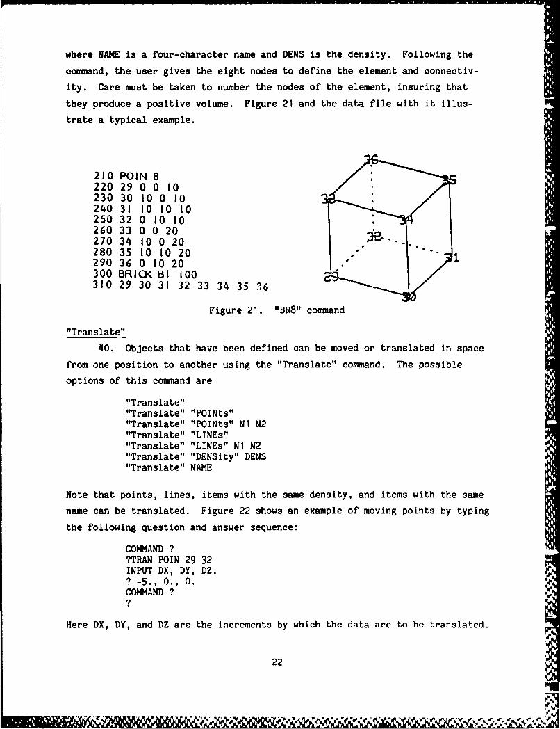
where NAME is a four-character name and DENS is the density. Following the

command, the user gives the eight nodes to define the element and connectiv-

ity. Care must be taken to number the nodes of the element, insuring that

they produce a positive volume. Figure 21 and the data file with it illus-

trate a typical example.

210 POIN 8220 29 0 0 10230 30 10 0 10240 31 10 10 10250 32 0 10 10260 33 0 0 20270 34 10 0 20280 35 10 10 20290 36 0 10 20300 BRIG< BI 100310 29 30 31 32 33 34 35 '6

Figure 21. "BR8" command

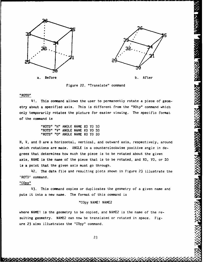
"Translate"

40. Objects that have been defined can be moved or translated in space

from one position to another using the "Translate" command. The possible

options of this command are

"Translate""Translate" "POINts""Translate" "POINts" Ni N2"Translate" "LINEs""Translate" "LINEs" Ni N2"Translate" "DENSity" DENS"Translate" NAME

Note that points, lines, items with the same density, and items with the same

name can be translated. Figure 22 shows an example of moving points by typing

the following question and answer sequence:

COMMAND ??TRAN POIN 29 32INPUT DX, DY, DZ.? -5., 0., 0.COMMAND ??

Here DX, DY, and DZ are the increments by which the data are to be translated.

22

a. Before b. After

Figure 22. "Translate" command

"IROTDII

41. This command allows the user to permanently rotate a piece of geom-

etry about a specified axis. This is different from the "ROtp" command which

only temporarily rotates the picture for easier viewing. The specific format

of the command is

"ROTD" "H" ANGLE NAME XO YO ZO"ROTD" "V" ANGLE NAME XO YO ZO"ROTD" "0" ANGLE NAME XO YO ZO

H, V, and 0 are a horizontal, vertical, and outward axis, respectively, around

which rotations are made. ANGLE is a counterclockwise positive angle in de-

grees that determines how much the piece is to be rotated about the given

axis, NAME is the name of the piece that is to be rotated, and XO, YO, or ZO

is a point that the given axis must go through.

42. The data file and resulting plots shown in Figure 23 illustrate the

'ROTD' command.

43. This command copies or duplicates the geometry of a given name and

puts it into a new name. The format of this command is

"COpy NAMEI NAME2

where NAMEl is the geometry to be copied, and NAME2 is the name of the re-

sulting geometry. NAME2 can now be translated or rotated in space. Fig-

ure 23 also illustrates the "COpy" command.

23

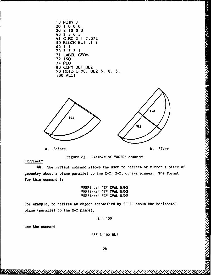
10 POIN 320 1 0 0 030 2 10 0 04.0 3 5 0 541 CIRC 2 I 7.07250 BLOCK BLI .1 260 I I70 3 3 2 I71 LABEL GEOM72 ISO74 PLOT80 COPY BLI BL290 ROTD 0 90. BL2 5. 0. 5.100 PLOT

DL24>~ IL

a. Before b. After

Figure 23. Example of "ROTD" command"REFlect"

44. The REflect command allows the user to reflect or mirror a piece of

geometry about a plane parallel to the X-Y, X-Z, or Y-Z planes. The format

for this command is

"REFlect" "X" XVAL NAME"REflect" "Y" YVAL NAME"REflect" "Z" ZAL NAME

For example, to reflect an object identified by "BLI" about the horizontal

plane (parallel to the X-Y plane),

Z = 100

use the comnand

REF Z 100 BLI

24

Similar commands would be used for reflection about planes X = XVAL and Y

YVAL. If "ALL" is given for NAME, the entire data base of geometry is

reflected.

45. The data file and resulting plots shown in Figure 24 further

illustrate the use of the REFlect command.

10 POINTS 720 1 80.436 0. 740.00030 2 88.250 0. 896.27040 3 100.000 0. 901.50050 4 169.370 0. 847.93060 5 212.966 0. 785.65070 6 244.976 0. 756.34480 7 244.976 0. 740.00090 ELLI 3 2 11.750 5.230 RIGH100 QUAD 3 4 134.685 0. 886.640110 CIRC 6 5 100.000 LEFT120 BLOCK OVE1 0.15500 49.000130 1.1140 7 1 2 3 4 5 6 7150 COPY OVE1 OVE2160 REFLECT X 0. OVE2

I

Figure 24. REFlect command example

"INPut"

46. This command allows the user to input or read into memory a perma-

nent data file saved on disc. Its format is

"INPut" FLNM1"INPut" FLNM1 "P"

25

where FLNM1 is a file description (20 characters maximum on Honeywell and 7

on CDC). If the P is also typed, a detailed printout of the input file

is also typed, a detailed printout of the input file is printed on the termi-

nal Just as if it had been done interactively.

"Volume"

47. This command allows the user to obtain volume information whenever

it is typed. Its format is

"Volume""Volume" "ALL""Volume" NAME

If "Volume" is typed, only the totals for the entire structure are given. If

"Volume" NAME is provided, only the volume data for data having the name are

given. "Volume" "ALL" will yield a detailed listing of the data by name; for

example,

NO. NAME VOLUME WEIGHT XCG YCG ZCG

1 BL1 3,141.59 314,159.27 0. 20.00 0.2 BL2 3,141.59 314,159.27 0. 20.00 25.00"1

TOTAL 6,383.19 628,318.53 0. 20.00 12.50

"ENd"

48. This command is given to terminate running of the program. Its

format is"ENd"

"GO"

49. This command is used when the program is being used for a specific

structure such as a dam or lock. Giving the "GO" command automatically caused

the program to go on from the General Geometry Module to the General Loads

Module. The format for this command is

"REturn"

50. This command is used to return to the question

STRUCTURE TYPE OF GENERAL MODULE?

so that the user can select another module. Typically, the next module is the

General Loads Module. The format for this command is

"REturn"

26 .

-Uk

"CLIP"51. The "CLIp" oomand allows the user to cut or clip the geometry by

an arbitrary plane to produce a new structure for use as a free-body diagram

or making new weight and centroid computations. The clipped data will be

placed into a new data file specified by the user. Blocks, bricks, or faces

not touched by the clipping plane will be placed untouched in the new file.

The parts left over from a clip however will be converted to faces with the

curved parts being modeled by bicubic patches and planar pieces having both

straight and cubic sides. The specific format of the conmand is

"CLIp X" XVAL NAME"CLIp +X" XVAL NAME"CLIp -X" XVAL NAME"CLIp Y" YVAL NAME"CLIp +Y" YVAL NAME"CLIp -Y" YVAL NAME"CLIp Z" ZAL NAME"CLIp +Z" ZVAL NAME"CLIp -Z" ZAL NAME"CLIp" LAB1 LAB2 LAB3 NAME

Note that you can clip parallel to the major axes or use three previously

defined points in space to define a plane to do the clippings. "CLIp X" XAL

means clip according to the vertical plane parallel to the YZ plane at a value

of X = XVAL, "CLIp Y" YVAL means clip according to the vertical plane parallel

to the XZ plane at a value of Y = YVAL, and "CLIp Z" ZAL means clip according

to the horizontal plane Z = ZVAL. A positive X, Y, or Z indicates that every-

thing in the positive direction past the specified plane should be kept and

the other clipped-off part thrown away, whereas a negative X, Y, or Z desig-

nation Indicates keeping in the negative direction. LAB1, LAB2, and LAB3 are

the labels of three previously defined points in space that determine the

clipping plane. The part that is kept is pointed to as a right-hand screw and

is advanced in the same way that the points are specified. NAME is optional

and specifies a specific piece of structure to be clipped. All other pieces

of geometry are left untouched and placed into the output file. If NAME is

not specified, the entire geometry is clipped.

52. When the "CLIp" command is given, the program asks for two output data

files where the new clipped data are to be placed. The first data file

contains the solid geometry description (blocks, bricks, faces, etc.), and the

27

Ne

second contains a definition of the resulting base or cross section of the in-

tersection of the clipping plane and the original geometry. After the clip io

complete, the program returns to the command level.

53. A sample data file (called SAMDAT) and the resulting interaction after

giving a "CLIp" command are shown in Figure 25 with before and after clips

plots.

10 POINTS S20 I 0. 0. 0.30 2 10. 0. 0.40 3 10. 0. 5.50 4 5. 0. 10.60 5 0. 0. 10.70 CIRC 4 3 S.80 BLOCK bIl .1 10.90 1. I.1005 54 32 1

CID~WO ?= I P SAMAOATCOM60M ? a. Before clip=CLIP Z 6.

ENTERING CLIPPING mXXLAE.

OUTPUT GEOMETRY LIATA FILE ?=CLGOM

OUfTPUT BASE DATA FILE ?CLIBAS

CLIPPING bil

EXITING CLIPPING mVoDLE. b. After clip

GCYWhAIV ?

Figure 25. "CLIp" command example

"CLEar"

54. This command is used to clear all definition of geometry from memory

to begin a new problem. Its format is

"CLEar"

"PLot"

55. This command allows part or all of the data base to be plotted. Its

format is

28 1

"PLot""PLot" "POINts""PLot" "POINts" N1 N2 4"PLot" "LINEs""PLot" "LINES" Ni N2"PLot" "DENSity" DENS"PLot" NAME

By typing "PLot", all the lines will be plotted. Thus, the default code is

"LINEs". By giving Ni and N2, a portion of the total number of lines can be

plotted. Points can only be plotted by typing "PLot" "POINts". If NI and N2

are given, only those points between N1 and N2 are plotted. Also, everything

with a given density (DENS) can be plotted. All data with a name (NAME) can

be plotted as well.

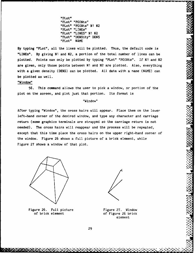
"Window"

56. This command allows the user to pick a window, or portion of the

plot on the screen, and plot just that portion. Its format is

"Window"

After typing "Window", the cross hairs will appear. Place them on the lower

left-hand corner of the desired window, and type any character and carriage

return (some graphics terminals are strapped so the carriage return is not

needed). The cross hairs will reappear and the process will be repeated,

except that this time place the cross hairs on the upper right-hand corner of

the window. Figure 26 shows a full picture of a brick element, while

Figure 27 shows a window of that plot.

Figure 26. Full picture Figure 27. Windowof brick element of Figure 26 brick tale

element %

2..929

".'k.'),"2.',',.?." ? .Pk-

"Zoom"

57. This command allows the user to decrease or increase the size of

the current picture on the screen. The format for this command is

"Zoom" FMAG

where FMAG is a scale factor which dictates whether the current picture is

made bigger or smaller. If FMAG is less than one, the picture is decreased in

size; if FMAG is greater than one, the picture is increased in size.

ffROtD"v

58. This command allows the user to rotate a picture of the structure

for viewing at different angles. This command is different from the "ROTD"

command which permanently rotates the geometry to a new position. The ROTP

coninand changes only the picture on the screen while the permanent storage of

the geometry is left untouched. Its format is

"ROtp" "H" ANGLE"ROtp" "V" ANGLE"ROtp" "O" ANGLE

where H means horizontal axis, V means vertical axis, and 0 means outward

axis. ANGLE is a counterclockwise, positive angle in degrees that determines

how much the structure is to be rotated about the given axis. Note, as shown

in the following example, the distinction between the coordinate system of the

X, Y, and Z data and that of that of the rotation axes. A good set of

rotation is"ROtp" "V" 30."ROtp" "H" 30.

"ISometric"

59. This command allows the user to specify a standard set of rotations

rather than search for the desired plot. Its format is

"ISometric"

It is equivalent to the two rotations given above.

"Label"

60. This command allows labels to be plotted along with line

30

V W'~S~i .% ~ - *.***** - ~ ~ . ~ .. ~-*****

segments. Two types of labels are available: (1) point labels and (2) name

lables. The format for this command is

"Label" "Points"

"Label" "Geometry"

Figure 28 illustrates the labeling of points by showing the results of typing

LABEL POINTSPLOT

Figures 23 and 24 show examples of labeling the names of geometric pieces,

LABEL POINTS

PLOT

Figure 28. "Label" "Points"

command

"Nolabel"

61. This command turns off the label options of the "Label" command.

Its format is

"Nolabel" "Points""Nolabel" "Geometry"

"Nolabel" is the default over "Label"."Dash"

62. This command allows the user to dash the lines that are hidden from

view. The format for this command is

"Dash"%.

Figure 29 shows the results of dashing the plot in Figure 26.

"Hide"

63. The command allows the user to delete hidden lines form the plot.

31

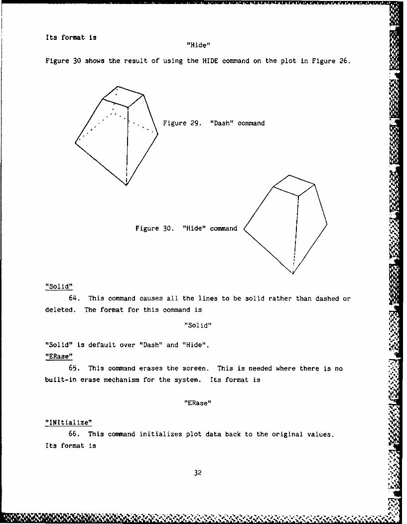
Its format is"Hide"

Figure 30 shows the result of using the HIDE command on the plot in Figure 26.

Figure 29. "Dash" command

Figure 30. "Hide" command

"Sol id"

64. This command causes all the lines to be solid rather than dashed or

deleted. The format for this command is

"Solid"

"Solid" is default over "Dash" and "Hide".

"ERase"

65. This command erases the screen. This is needed where there is no

built-in erase mechanism for the system. Its format is

"ERase"

"INItialize"

66. This command initializes plot data back to the original values.

Its format is

32

"INItialize"

Currently, the angles of rotation are reset to zero.

Practical Applications

67. The applicability of this program can be studied in further detail

with the plates herein. Additional study and research have been done by

Mr. Obbie Thompson, Jr.,* US Army Engineer District, St. Louis, though the

material has not been published. Plates 1 and 2 are plots provided by Messrs.

Thomas J. Mudd* and John Jobst,* US Army Engineer District, St. Louis, illus-

trating practical applications of this program. Plate 3 was provided by

Mr. Steve Freitas,** Sacramento District. These plates are placed at the end

of the main text of this report.

.p.

*The contributions by Messrs Thompson, Mudd, and Jobst, US Army Engineer,District, St. Louis, are the result of preliminary work in preparation for :Design Memorandum No. 17, 1978 (Dec), John H. Overton Lock and Dam, RedRiver Waterway.

**The plate furnished by Mr. Steve Freitas, US Army Engineer District,Sacramento, has never been published.

33

.'4

• & -.. , . . . .. . .. .-. . . .. ._ ..- . - .-. -. . -. . .. . . .° .. . . . ° .. . . .- - . .. . .-. -.. ..-

REFERENCES

Johnson, Robert H. 1984. Solid Modeling: A State-of-the-Art Report, CAD/CAMALERT, Management Roundtable, Inc., Chestnut Hill, Mass.

Tracy, Fred T. 1980. "A Three-Dimensional Analysis/Design Program (3DSAD),General Geometry Module," Instruction Report K-80-4, Report 1, US Army Engi-neer Waterways Experiment Station, Vicksburg, Miss.

Tracy, Fred T., and Kling, Charles W. 1982. "A Three-Dimensional Analysis/Design Program (3DSAD), General Analysis Module," Instruction Report K-80-4,Report 3, US Army Engineer Waterways Experiment Station, Vicksburg, Miss.

Tracy, Fred T., Kling, Charles W., and Holtham, William J. 1983. "A Three-Dimensional Analysis/Design Program (3DSAD), Special Purpose Modules for Dams(CDAMS)," Instruction 'Report K-80-4, Report 4, US Army Engineer WaterwaysExperiment Station, Vicksburg, Miss.

Wilson, Howard B., Jr., and Farrior, Donna S. 1976. "Computation of Geo-metric and Inertial Properties for General Areas and Volumes of Revolution,"Computer Aided Design, Vol 8, No. 4.

34

V Nc

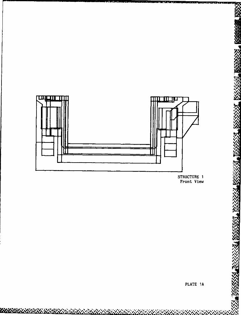
STRUCTURE 1Front View

PLATE 1A

STRUCTURE 1Overhead View

PLATE 1B

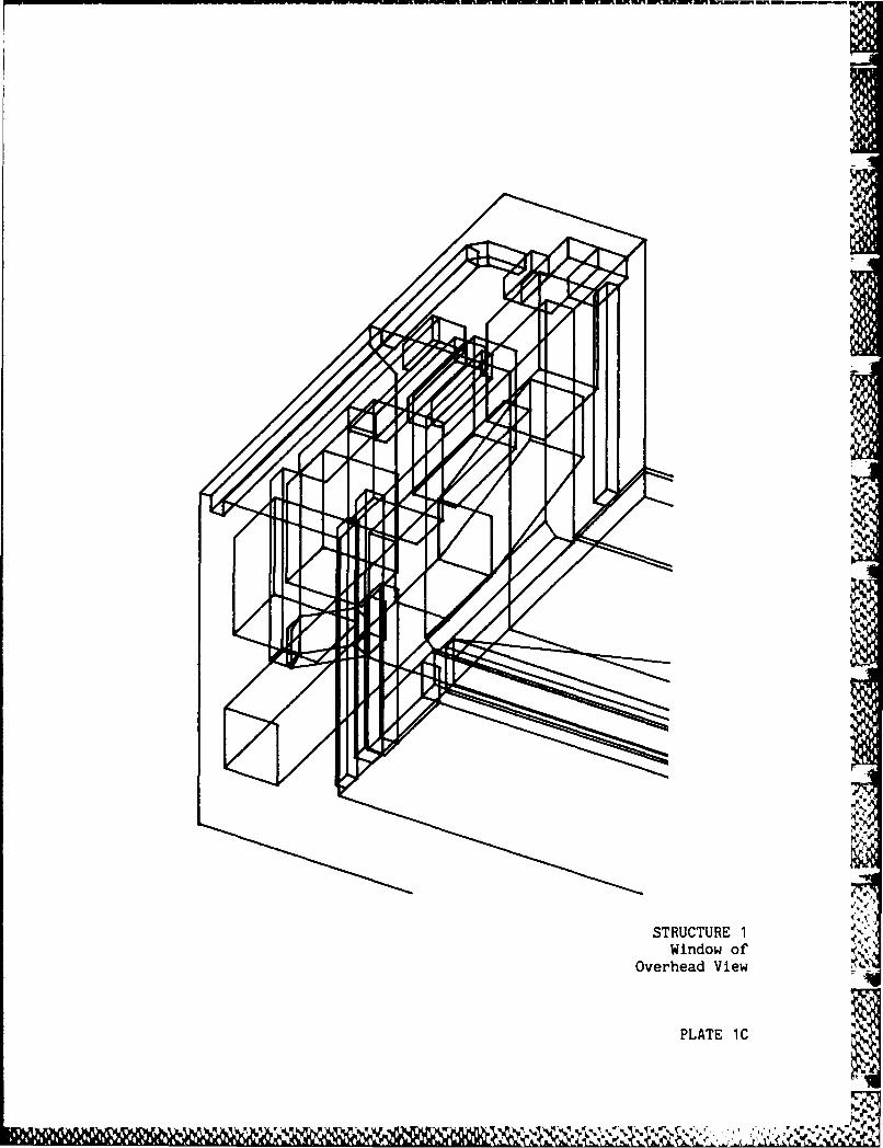
STRUCTURE 1Window of

Overhead View

PLATE 1C

STRUCTURE 1First Block

PLATE 1D

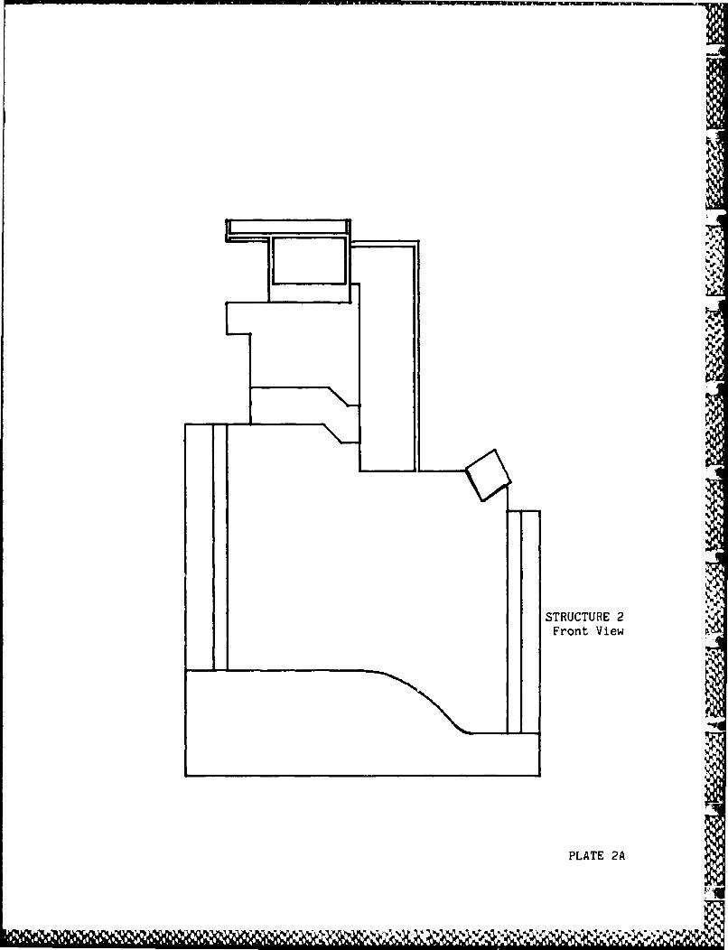
STRUCTURE 2Front View

PLATE 2A

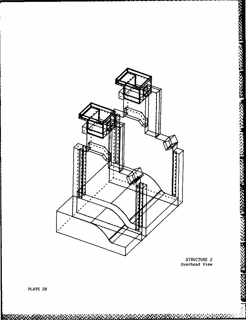
STRUCTURE 2Overhead View

L6

PLATE 2B

I

QN

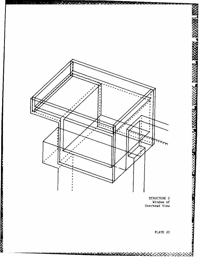
STRUCTURE 2Window of'

Overhead View

PLATE 2C

lop

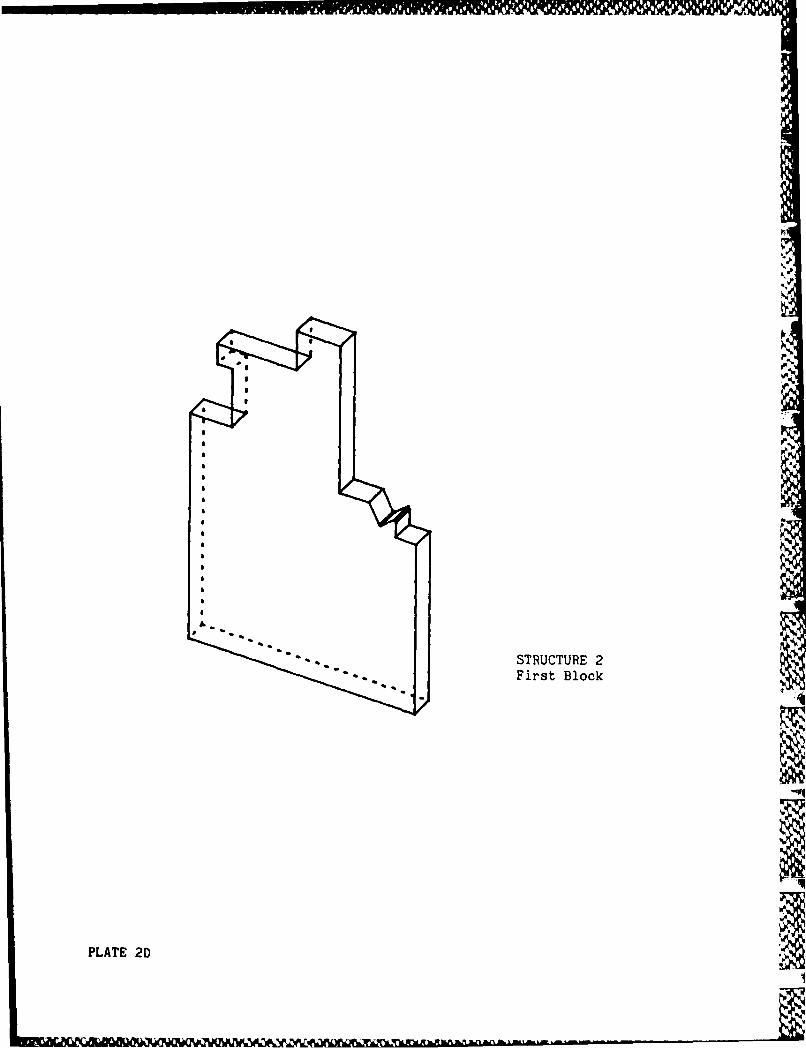
STUTRa

Fis lc

MII

PLATE 2

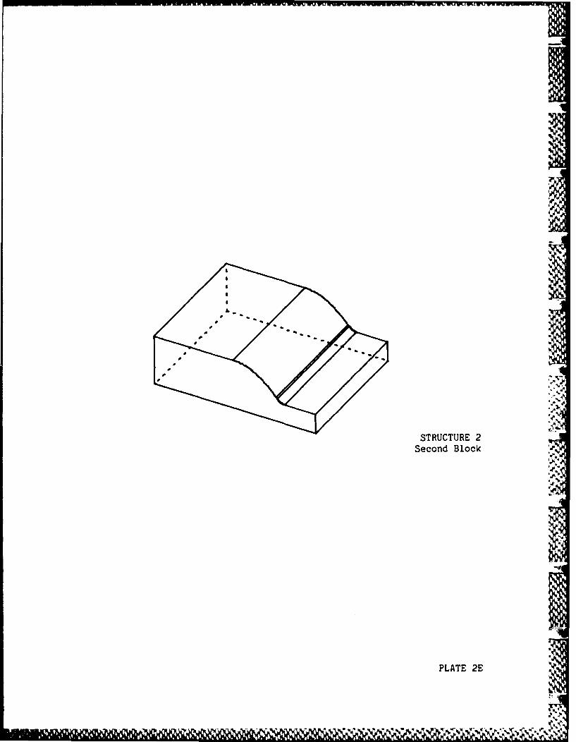
1WIMMM ]PI ~wm"I

STRUTUR 2.8Secon Bloc

PLATE 2E

a 11 11 I III, I N ,

.

0 i I li

II II0"t

APPENDIX A: THEORY AND PROCEDURE FOR

COMPUTING MASS PROPERTIES

Introduction

1. A Three-Dimensional Stability Analysis/Design (3DSAD) Program (Tracy

1980;* Tracy and Kling 1982; Tracy, Kling, and Holtham 1983) for analyzing and

designing concrete structures has been developed and successfully used. This

program models the geometry and loads in a general way and then applies this

modeling capability to specific structures types whenever possible. Examples

include dams with overflow, nonoverflow, and pier sections; gravity and

U-frame locks; cooling towers; etc. Even if the structure does not conform to

a predefined standard shape, the program can do a general analysis of the

problem because of the fundamental approach of using solid modeling type capa-

bility as a foundation.

2. There are several ways to model geometry and many commerical pack-

ages exist for this (Johnson 1984). The approach taken in 3DSAD was to first

provide some of this capability internal to the program and at a later date

supply the capability to tie 3DSAD into the larger system.

Modeling Technique

3. 3DSAD models geometry in three ways:

a. Blocks--Two-dimensional (2-D) cross sections swept normal to thecross section in a linear or axisymmetric way with linear andquadratic tapering for the linear sweeps.

b. Eight-node brick elements.

c. A boundary representation consisting of planar faces and bicubicpatches.

Mass Properties--BLOCK a

4. One of the major points of this appendix is to describe the

* References cited in this appendix are included in the References at the endof the main text.

Al

Lama"

equations for performing mass properties for blocks. The blocks are formu-

lated by first defining a cross section, then parametrically performing a

constant or tapered linear sweep or an axisymmetric sweep. Thus, area inte-

grals can first be computed, and from these the mass properties can be figured

by performing the integration in the third dimension.

5. For a cross section defined by a polygon, it is best to convert the

area integrals to line integrals (Wilson and Farrior 1976). For a cross sec-

tion consisting of both courved and straight line segments, it is tempting to

first approximate the curved edges with straight line segments and then the

line integrals. However, this process is time consuming and creates unneces-

sary errors, since it is possible to formulate line integrals for curved edges

as well. This appendix presents examples of these line integrals developed in

a consistent manner.

6. The volume of a block with constant cross section (Figure Al)

having j sides can be expressed as

V = -Lf C YdX

n

= -L YdX

n

: jzl ,

W.,

Figure Al. Blocks with constant cross section ?.

A2A

V %*

N

• " = -- -" ,"%' '%'% %'" % %- -. %-.%-, %-N,.%.-.. .. N ,% %° % .. ... .. , , ,... a,

The integral Ii can now be evaluated for different line segments types.

7. Linear line segment. Suppose the line segment is defined by twopoints (X1 , Y) - (X2 , Y2 ). Then

X =X + (X2 - X1 )S

+ ~2 1Y =YI + (Y2 -YIO s

where S varies between 0 and 1. I can be done as:

I f[Y 1 + (Y2- Y1 ) S] (X2- X1) dS

0

1 1 k

fA 1 L BkS dS0 k= k

1 BA1 kk+ 1

8. Quadratic line segment. In a similar manner, a quadratic line

segment formed by three points, 1, 2, and 3, can be expressed as:

r1x [X1 x2 x -3 S 2

2 Akk

k=O

2

1= kY: BSm

m=O m -

dX E (k + 1)Ak+1 S dSk:O

Here M is the "magi-" matrix of known constants, and as in the linear case, A

and B are constants of the parametric polynomials. The line integral I can

now be easily evaluated as follows:

A3

P.'

. L A2.1 -t. -' "

2 k]

I: = ,= Bm) [= (k + 1) A k+ Sk dS

2 k+ 1 A B

k + m + 1 k+1 mm=O k=O

Note also at this point that higher order integrals, the X centroid, for

example, can be done with equal ease.

VC

2 2 1 k+ ABAE E L k+ m + n + 1 'm n k+lm=O n=O k=O

The general trend is now set with the form being the same for any poly-

nomial. Also, another X or Y inside the integral simply results in

another summation sign.

9. Circular arc. The circular arc can also be put in the same

consistent notation with use of complex variables as:

X = R cos (AS + 0O)

Y = R sin (AS + 0O)

W: eiAS

1 . %kX = AkWk

k=-1

1Y F B Wm

M=-, 11k

dX = iA kAkW dSk=-1

With this foundation the line integrals can be figured as easily as the

polynomials.

A4

I f Bm)A k kAkW dS .ll(A k A

m=-1 k=-e

10. Elliptical arc. An elliptical arc can also be handled in the same

consistent manner.

X = A cos (OS + o )

Y = B sin (OS + eO)

X E AkW k

k=-l

1YB W....

m=- 1.

11. Tapered block. Consider now a cross section defined in the X-Y

plane. Let (Xo, Yo) be a point on that cross section. The (X, Y) value of . .

a point on a cross section at elevation Z as a result of a taper is -

X(Z) = (X0 - XA)SX(Z) + XA

Y(Z) (Yo- YA)Sy(z) Y

where (XA, YA) is an apex point, and Sx(Z) and S (Z) are scale factors that

range in value from 0 to 1. The scale factor functions determine the type of

tapering. Let Z vary from 0 to L and let the scale factor functions

vary quadratically:

Z = LS

A5

s X4 HX FX]~ []

: AjSS12

2= A Si

2 kk:O k

where Hx and Fx are the values of the X scale factor, respectively, for

S = 0.5 and S 1 . Let a similar expression for the Y scale factor also

be defined. Let A be the area of the cross section at elevation Z Then

the volume is completed by

A : A0 SX S y

V ' LAdZ

SA 0 AiS) BkS) L dS

A L 2 2 A B

0 E E i ,j k+1 kJ=O k:O

Mass Properties--FACES

12. Two types of faces will be considered: tA

a. Planar face

b. Bicubic patch

13. Planar face. By using the equation of the plane, the mass property K

integrals for planar faces can also be converted to line integrals and then

computed as before. For example, the volume under a planar face can be

computed as:

A6 U

v Z dX dYA

f. (AX + BY + C) dX DY

- -f (AX + .5BY'+ C) YdX

These volumes, when summed over all the faces, will give the correct volume

for the solid.

14. Bicubic patch. Bicubic patches can be defined in several ways.

Whatever the boundary conditions or formulation, they can typically be cast:

3 3 A S i T j

i=O J=O

3 3Y A S k T1

i1

k=O 1=0

3 3

z= L : C rn

m=O n=O

Mass properties can be computed with numerical integration or exact

formulation. The exact formulation is:

V f Z dX dY

So Z IJf dS dT

3 3 3 3 3 3F E E E L TE Tijklmn

i=O J=O k=O 1=0 m=0 n=m

T iJklm n (il - Jk)A ijB klCmn: (i + k + m) (j + 1 + n)

A7

WATERWAYS EXPERIMENT STATION REPORTSPUBLISHED UNDER THE COMPUTER-AIDED

STRUCTURAL ENGINEERING (CASE) PROJECT

Title C

Technical Report K-78-1 List of Computer Programs for Computer-A-ded StruCtural Engint-rr Feb 191M

Instruction Report 0-79-2 User's Guide. Computer Program with Interactive Graphics tor Ma~ r5Analysis of Plane Frame Structures 1CFRAMEi

Technical Report K-80-1 Survey of Bridge-Oriented Design Software ;;un '980O

Technical Report K-80-2 Evaluation Of Computer Programs for the Design Aralyrlsuf .sHighway and Railway Bridges

lnstrUctio- Report K-80-1 User's Guide. Computer Program tor Dfws-ign.H )ei-vf Cr-linear Concuits/'Culverts ICURCON p

nstructir Report K-80-3 A Thre,,e-Dimensional Finite Element Data Edi! ProtrarM

IrS trl.uCtior Report K-80 4 A Three- Dimfensional Stuourity Analysis. Desi Prog-;,rm 3 DSACReport 1. General Geometry MoclReport 3 General Analysis ModleI (GGAM, -:

Report 4 Special-Purpose Modules for Darns (CDAMSj 1'I 'SO ti mI'eport K-80-6 Basic User's Guiide. Computer Programi for Design arnc Anal-isl ii

At lnvere- Retaining Wails and Floodwalis (TWDA)

Ie ctrRepj.,rt K-80- 7 Users Reference Manual Computer Program for Design arid 9 1%

Aniaiysis of Inverted T Retaining Wall-, and Ploodwalis TWiA,

Tceimc Rep,,rt K-80-4 Documertation of Fintite Element AnalysesReport 1. Lorngview Outlet Works Conduit Le fkReport 2. Anchored Wall Monolith, Bay Springs Lock -c 4

Tiu~rr~cK Keoi~8-5 Basic Pile Group Behavior

r i; cr P ~p ,t n,r" 1- User's Guide Computer Program for Des-ign arc AnmiVcs Lof S5(cPiie Walls hy Classiosi Methods 1CSHTWAL)

*Report 1 Computational Processes,Report 2 Interacr.tive Graphcs Options

'<W ri 0 ~- 0 f ~_ ~liidat~niReprrComiputer Program fo)r Dosq . o1 rav;r*Inverted- T 'ciN ail, aind Floodwas T Wi

I'.trmI onRpor K eu 4 0s- s G e lop itrrr Programi for a9sg ri: A'viOyyis oCast-in-Piace I nn' t '-rirq (NEW I1U fi

RI ":: Ln i -I tf .81-6 ijs; r s Cuijlde pin Pr ,;rm '0 Lip r') ri r'5y4 r .

'rt r ;iKl--f, '

0 ri t'0-

-T *-, t-

t.

fill - . -

WATERWAYS EXPERIMENT STATION REPORTSPUBLISHED UNDER THE COMPUTER-AIDED

STRUCTURAL ENGINEERING (CASE) PROJECT

(Concluded)

Title Date

Instruction Report K-83-1 User's Guide: Computer Program With Interactive Graphics for Jan 1983Analysis of Plane Frame Structures (CFRAME) F-

Instruction Report K-83-2 User's Guide: Computer Program for Generation of Engineering Jun 1983Geometry (SKETCH)

Instruction Report K-83-5 User's Guide: Computer Program to Calculate Shear, Moment, Jul 1983and Thrust (CSMT) from Stress Results of a Two-DimensionalFinite Element Analysis

Technical Report K-83-1 Basic Pile Group Behavior Sep 1983

Technical Report K-83-3 Reference Manual: Computer Graphics Program for Generation of Sep 1983Engineering Geometry (SKETCH)

Technical Report K-83-4 Case Study of Six Major General-Purpose Finite Element Programs Oct 1983

Instruction Report K-84-2 User's Guide: Computer Program for Optimum Dynamic Design Jan 1984of Nonlinear Metal Plates Under Blast Loading (CSDOOR)

Instruction Report K-84-7 User's Guide: Computer Program for Determining Induced Aug 1984Stresses and Consolidation Settlements (CSETT)

Instruction Report K-84-8 Seepage Analysis of Confined Flow Problems by the Method of Sep 1984Fragments (CFRAG)

Instruction Report K-84-11 User's Guide for Computer Program CGFAG, Concrete General Sep 1984Flexure Analysis with Graphics

Technical Report K-84-3 Computer-Aided Drafting and Design for Corps Structural Oct 1984Engineers

Technical Report ATC-86-5 Decision Logic Table Formulation of ACI 318-77, Building Code Jun 1986Requirements for Reinforced Concrete for Automated Con-straint Processing, Volumes I and II

Technical Report ITL-87-2 A Case Committee Study of Finite Element Analysis of Concrete Jan 1987Flat Slabs

Instruction Report ITL-87-1 User's Guide: Computer Program for Two-Dimensional Analysis Apr 1987of U-Frame Structures (CUFRAM)

Instruction Report ITL-87-2 User's Guide: For Concrete Strength Investigation and Design May 1987(CASTR) in Accordance with ACI 318-83

Technical Report ITL-87-6 Finite-Element Method Package for Solving Steady-State Seepage May 1987Problems

Instruction Report ITL-87-3 User's Guide: A Three Dimensional Stability Analysis/Design Jun 1987Program (3DSAD), Report 1, Revision 1. General GeometryModule

--- - ,