A&A 626, A53 (2019)https://doi.org/10.1051/0004-6361/201935539c© ESO 2019

Astronomy&Astrophysics

MHD simulations of the in situ generation of kink and sausagewaves in the solar corona by collision of dense plasma clumps?

P. Pagano1, H. J. Van Damme1, P. Antolin1, and I. De Moortel1,2

1 School of Mathematics and Statistics, University of St Andrews, North Haugh, St Andrews, Fife KY16 9SS, UKe-mail: pp25@st-andrews.ac.uk

2 Rosseland Centre for Solar Physics, University of Oslo, PO Box 1029, Blindern 0315, Oslo, Norway

Received 25 March 2019 / Accepted 29 April 2019

ABSTRACT

Context. Magnetohydrodynamic (MHD) waves are ubiquitous in the solar corona where the highly structured magnetic fields provideefficient wave guides for their propagation. While MHD waves have been observed originating from lower layers of the solar atmo-sphere, recent studies have shown that some can be generated in situ by the collision of dense counter-propagating flows.Aims. In this theoretical study, we analyse the mechanism that triggers the propagation of kink and sausage modes in the solar coronafollowing the collision of counter-propagating flows, and how the properties of the flows affect the properties of the generated waves.Methods. To study in detail this mechanism we ran a series of ideal 2D and 3D MHD simulations where we varied the propertiesof the counter-propagating flows; by means of a simple technique to estimate the amplitudes of the kink and sausage modes, weinvestigated their role in the generation and propagation of the MHD waves.Results. We find that the amplitude of the waves is largely dependent on the kinetic energy of the flows, and that the onset of kinkor sausage modes depends on the asymmetries between the colliding blobs. Moreover, the initial wavelength of the MHD waves isassociated with the magnetic configuration resulting from the collision of the flows. We also find that genuine 3D systems respondwith smaller wave amplitudes.Conclusions. In this study, we present a parameter space description of the mechanism that leads to the generation of MHD wavesfrom the collision of flows in the corona. Future observations of these waves can be used to understand the properties of the plasmaand magnetic field of the solar corona.

Key words. Sun: oscillations – Sun: corona – Sun: helioseismology – magnetohydrodynamics (MHD) – Sun: magnetic fields

1. Introduction

Magnetohydrodynamic (MHD) waves are an intrinsic feature ofthe solar corona, and for this reason have been studied in detailsince the derivation of their existence (for a review, see e.g.De Moortel & Nakariakov 2012; Arregui 2015). The solarcorona is a highly dynamic and structured environment wheremagnetic fields are often concentrated in coronal loops andactive regions. The formation process of coronal loops is stillunder investigation, but these magnetised structures are efficientwave guides for MHD waves (Reale 2010).

This scenario has been observed a number of times and aphotospheric or chromospheric origin has been suggested formost of the MHD waves propagating along these wave guides, asthese modes are powered by the upward Poynting flux observedat the lower layers of the solar atmosphere (e.g. Matsumoto &Kitai 2010; Chitta et al. 2012; Krishna Prasad et al. 2015). At thesame time, Morton et al. (2019) have shown that the power spec-trum of the transverse oscillations in the corona is relatively sta-ble and uniform throughout different regions and the solar cycle,suggesting that these oscillations must be fundamentally con-nected with the pulsation of the lower layers of the Sun’s atmo-sphere. However, various observational and theoretical stud-ies have recently been suggested that not all the transversewaves observed in the solar corona are of chromospheric origin,? The movies associated to Figs. 2 and 21 are available athttps://www.aanda.org

but that some are generated in situ. For instance, a series of stud-ies (Kohutova & Verwichte 2018, 2017; Verwichte et al. 2017;Verwichte & Kohutova 2017) have found that coronal rain can bean efficient source for these waves in coronal loops. When gen-erated at photospheric level, Alfvénic waves suffer from strongreflection when travelling through the lower layers of the solaratmosphere. Therefore, a mechanism that allows in situ wavegeneration bypasses this problem, and constitutes an additionaland potentially important source of energy for the corona.

Antolin et al. (2018, hereafter Paper I) have shown howMHD waves can be generated from the interaction of counter-propagating flows or clumps of plasma along coronal loops. Itis not clear yet how frequently this mechanism is, but the sce-nario seems particularly plausible in loops with coronal rain (e.g.Antolin & Rouppe van der Voort 2012; Kleint et al. 2014), inprominences (e.g. Alexander et al. 2013), or when strong plasmaevaporation is present (e.g. Brosius & Phillips 2004; Brosius2013; Gupta et al. 2018).

In Paper I we focus on the observation and modelling ofa specific event observed on 2014 April 3 during a coordi-nated observing campaign between the Interface Region Imag-ing Spectrograph (IRIS, De Pontieu et al. 2014) and Hinode(Kosugi et al. 2007), combined with support from the SolarDynamics Observatory (SDO, Pesnell et al. 2012), pointingat a prominence and coronal rain complex on the west limbof the Sun. The observations clearly show two rain clumpsmoving along the same coronal structure in opposite direc-

Article published by EDP Sciences A53, page 1 of 12

A&A 626, A53 (2019)

tions. When the two clumps intersect in the plane of the sky(POS), a localised brightening is observed. At this point thetwo clumps merge into one and continue moving downwardsalong the same structure, and a transverse oscillation of therain strand is observed in the POS. The analysis of the obser-vations combined with the modelling have led us to interpretthese observations as coupled kink and sausage modes triggeredby the collision of the two clumps.

The model devised for this purpose consisted of an ideal 2DMHD simulation of two asymmetric clumps travelling towardseach other in a uniform medium. The parameters of the MHDsimulations were chosen to match the observations, and themagnetic field strength was picked to retrospectively matchthe observed kink amplitude. While the model was suitableto explain one specific observation, it has triggered new ques-tions about this mechanism as a way to generate transverseMHD waves in the solar corona. In particular, the connectionbetween the properties of the clumps and the properties of theinduced transverse modes has not yet been clarified, nor hasthe evolution of the forces during the collision. A key openissue is the degree of asymmetry required to trigger kink modes,and whether sausage modes are also a common result. From amore general perspective, the primary question that needs to beanswered in this and future studies is whether the excitation ofMHD waves in the solar corona through flow collision is a com-mon event or a rare phenomenon. This has important implica-tions for the energy budget, and the fraction originating fromthe lower layers of the solar atmosphere. Additionally, this is apotentially very interesting tool for seismology studies.

The main focus of this work is to explain how the interac-tion of counter-propagating clumps in coronal loops can lead tothe generation of transverse MHD waves. Also, we explore howthe properties of the clumps can influence the properties of theexcited kink and sausage modes. In order to do that, we startfrom the MHD simulations already presented in Paper I, and sig-nificantly expand that investigation by varying the key parame-ters of the clump collisions. We also extend the model to 3D, andinvestigate the changes relative to the 2D case.

The paper is structured as follows: in Sect. 2 we present the2D MHD simulations used for our modelling; in Sect. 3 weanalyse in detail how the collision of two counter-propagatingclumps generates MHD waves; in Sect. 4 we expand the study byexploring the parameter space of the clump properties; in Sect. 5we analyse how our results change in a 3D set-up; and in Sect. 6we present our conclusions.

2. Model

To study the generation of transverse MHD waves in the solarcorona from counter-propagating plasma flows, we devised asimple MHD model. This model is capable of reproducing someobserved features, as demonstrated in Paper I. Two dense clumpsare set to travel in opposite directions to reproduce the observedupward and downward travelling features, and the properties ofthe background plasma and magnetic field are chosen so thatobserved properties of the transverse waves following the inter-action are reproduced.

We repeat here only the most important properties of ourMHD model, and we refer the reader to Paper I for furtherdetails. We perform our numerical experiment in a Cartesian 2Ddomain and we solve the ideal MHD equations using the MPI-AMRVAC software (Porth et al. 2014):∂ρ

∂t+ ∇ · (ρu) = 0, (1)

∂ρu

∂t+ ∇ · (ρuu) + ∇p −

j × Bc

= 0, (2)

∂B∂t− ∇ × (u × B) = 0, (3)

∂e∂t

+ ∇ · [(e + p)u] = 0, (4)

where t is time, ρ density, u velocity, p the gas pressure, B themagnetic field, j = c

4π∇ × B the current density, and c the speedof light. The total energy density e is given by

e =p

γ − 1+

12ρu2 +

B2

8π, (5)

where γ = 5/3 denotes the ratio of specific heats.The initial conditions are described in a Cartesian reference

frame where the x-direction is aligned with the initial uniformmagnetic field B = 6.5 G. The simulation domain extends fromx = −6 Mm to x = 6 Mm and from y = −3 Mm to y = 3 Mm.The background plasma has a density of ρ = 10−15 g cm3, cor-responding to a number density n = 1.2 × 109 cm−3 in a fullyionised plasma (or an electron density ne = 6 × 108 cm−3), anda uniform temperature of Te = 1 MK, leading to a plasma ofβ = 0.098. Although coronal rain is not a fully ionised plasma(Antolin & Rouppe van der Voort 2012), we do not expect thisassumption to have a significant effect on the study carried outhere. Oliver et al. (2016) found that even in the extreme case of50% partially ionised plasma, the neutrals are still strongly cou-pled to the ions. The clumps are in pressure equilibrium with thebackground, but have a density ρC times higher and thus a tem-perature of T = Te/ρc K. The clumps are travelling at a speed VCin opposite directions. Each clump has a trapezoidal shape ori-ented so that the two opposite faces are parallel to one anotherwith an angle θ of inclination between these faces and the direc-tion perpendicular to the direction of travel (i.e. y-direction). Theinitial distance of the clumps is d = 3 Mm.

The numerical experiment runs for 300 s which is sufficientlylong for the collision between the clumps to occur and for thesystem to approach a new equilibrium in the aftermath of thecollision. The boundary conditions are treated with a system ofghost cells where we set zero gradient for all MHD variables atboth x and y boundaries.

3. Simulation

As the main focus of this work is to describe the interactionof counter-propagating clumps in a coronal loop, in this sectionwe illustrate in detail one of the characteristic simulations pre-sented in Paper I. This section significantly expands the analysisdescribed in Paper I, and it is essential to introduce the sub-sequent parameter space investigation. In particular, we illus-trate in detail the mechanism through which MHD waves aregenerated in our numerical experiment. Figure 1 shows the ini-tial condition of this numerical experiment where two denseclumps are aligned and travelling at the same speed in oppositedirections.

In this representative simulation, two clumps of trapezoidalshapes are set to travel towards each other at a speed of vC =70 km s−1. The two clumps have a density contrast ρC = 100,their width is w = 1 Mm, their length at the centre is L = 3 Mm,and the angle of the facing clump surfaces is θC = 50◦. Thisset-up was found to produce the best match with the observeddynamics (Paper I).

A53, page 2 of 12

P. Pagano et al.: Waves from collision of dense clumps

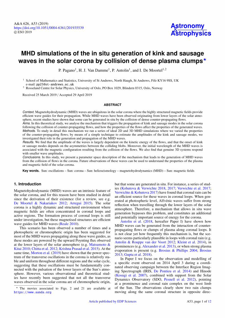
Fig. 1. Map of the number density n at t = 0 s. Green lines are magneticfield lines drawn from the left-hand boundary. Blue and red lines are thespecific external (red) and internal (blue) pairs of magnetic field linesused in Sect. 3.2.

3.1. Collision

The initial speed of the clumps relative to the backgroundmedium is lower than both the Alfvén speed (VA = 600 km s−1)and the sound speed (Cs = 165 km s−1), thus no shock initiallydevelops and the two clumps travel at constant speed in oppositedirections. In doing so, their motion leads to a compression ofthe plasma ahead of their propagation and a rarefaction behind.

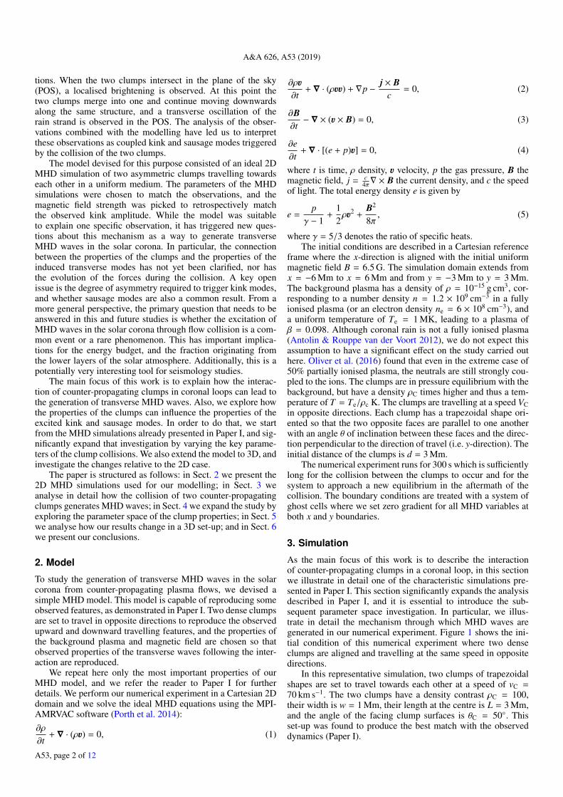
At t = 7 s the two compressed regions touch and the col-lision phase begins. Figures 2a–c show ρ, T , and p of the sys-tem at t = 25 s, an intermediate stage during the collision. Atthis time the clumps have started to change shape at their frontsbecause of the interaction. In particular, the front of the clumpshas expanded in the y-direction and the magnetic field lines havefollowed this deformation. It should be noted that the magneticfield is most deformed where the two clump surfaces are touch-ing, thus at different x-coordinates for the upper and lower sidesof the clumps because of their asymmetric shape. At this stage,the compression between the clumps has caused a significantincrease in both pressure and temperature. The latter reachesabout T = 3 MK, which is its maximum over the course ofthe simulation. This high temperature is maintained only for afew seconds before it drops again. At this time, the gas pressuredistribution between the clumps follows the pattern of the twocolliding fronts and strong gradients are generated along the col-lision region. Over the same region, the y-velocity of the plasmais directed outwards (vy ∼ ±10 km s−1) with respect to the colli-sion and the magnetic field is displaced with the plasma.

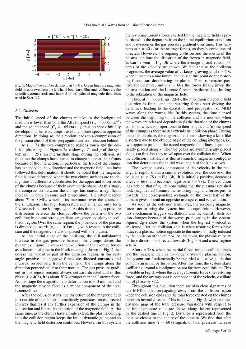
At this initial stage of the collision, the still unbalancedincrease in the gas pressure between the clumps drives thedynamics. Figure 3a shows the evolution of the average forcesas a function of time in the black rectangle shown in Fig. 2 thatcovers the y-positive part of the collision region. In this rect-angle positive and negative forces are directed outwards andinwards, respectively, from the centre of the clumps along thedirection perpendicular to their motion. The gas pressure gradi-ent in this region remains always outward directed and in thisphase (t < 40 s), it is about 30% stronger than the Lorentz force.At this stage the magnetic field deformation is still minimal andthe magnetic tension force is a minor component of the totalLorentz force.

After the collision starts, the distortion of the magnetic fieldjust outside of the clumps immediately generates forces directedinwards that resist any further expansion of the clumps in they-direction and limits the distortion of the magnetic field. At thesame time, as the clumps have a finite extent, the plasma cominginto the collision region keeps the initial dynamic going and sothe magnetic field distortion continues. However, in this system

the restoring Lorentz force exerted by the magnetic field is pro-portional to the departure from the initial equilibrium conditionand it overcomes the gas pressure gradient over time. This hap-pens at t = 40 s for the average forces, as they become inwarddirected. However, the ongoing collision and the inertia of theplasma continue the distortion of the frozen in magnetic field,as can be seen in Fig. 3b where the average vx and vy compo-nents of the velocity are shown. We find that as the collisionprogresses, the average value of vy keeps growing until t = 60 swhen it reaches a maximum, and only at this point do the restor-ing forces start decelerating the plasma. Then, vy remains pos-itive for 6 s more, and at t = 66 s the forces finally invert theplasma motion and the Lorentz force starts decreasing, leadingto the relaxation of the magnetic field.

Thus, at t = 66 s (Figs. 2d–f), the maximum magnetic fielddistortion is found and the restoring forces start driving thedynamics, leading to the excitation and propagation of MHDwaves along the waveguide. In this system, the time elapsedbetween the beginning of the collision and the moment whenthe waves are released depends on (i) the duration of the clumpscollision, which is proportional to their length, and (ii) the speedof the clumps as their inertia extends the collision phase. Duringthe collision phase, the magnetic field starts showing a kink-likedistortion due to the oblique angle of the colliding interfaces, i.e.two opposite peaks in the traced magnetic field lines, asymmet-rically placed along x. The two peaks are symmetrically placedalong x at first, but they travel apart over the collision time. Whenthe collision finishes, it is this asymmetric magnetic configura-tion that determines the initial wavelength of the kink waves.

The average x-axis component of the velocity in the rect-angular region shows a similar evolution over the course of thecollision (t < 78 s in Fig. 3b). It is initially positive, decreasesafter t = 66 s, and becomes negative at t = 78 s. This evolutionlags behind that of vy, demonstrating that the plasma is pushedback (negative vy) because the restoring magnetic forces push itinwards. The corresponding rectangle on the lower half of thedomain gives instead an opposite average vy and vx evolution.

As soon as the collision terminates, the restoring magneticforces act to bring the system back to equilibrium. However,this mechanism triggers oscillations and the density distribu-tion changes because of the waves propagating in the system.Figures 2g–i show the system when the highest y-velocitiesare found after the collision, that is when restoring forces haveinduced a plasma motion opposite to the motion initially inducedby the collision of the clumps. At this point, the plasma velocityin the y-direction is directed inwards (Fig. 3b) and a new regimesets in.

After t = 78 s, when the inertial force from the collision endsand the magnetic field is no longer driven by plasma motion,the system can fundamentally be regarded as a wave guide thatcontains an initial perturbation. After this time, the system startsoscillating around a configuration not far from equilibrium. Thisis visible in Fig. 3, where the average Lorentz force (the restoringforce) and the average y-axis component of the velocity oscillateout of phase by π/2.

Throughout this evolution there are also clear signatures offast MHD modes propagating away from the collision regionwhen the collision ends and the total force exerted on the clumpsbecomes inward directed. This is shown in Fig. 4, where a time-distance map of the total pressure variations with respect tothe initial pressure value are shown along the cut representedby the dashed line in Fig. 2. Distance is represented from thelocation closest to the centre of the domain. We find that afterthe collision time (t = 60 s) signals of total pressure increase

A53, page 3 of 12

A&A 626, A53 (2019)

Fig. 2. Maps of number density, temper-ature T , and gas pressure p at differenttimes of the MHD simulation. In the ρmaps, green lines are magnetic field linesdrawn from the left-hand boundary. Therectangular box shows the region overwhich we average quantities for Fig. 3,and the white dashed line is the cut weuse to plot the time-distance diagram inFig. 4. A movie is available online.

Fig. 3. Panel a: evolution of the y-axis components of the gas pressuregradient (−∇Py, red solid curve), Lorentz force (LFy, blue solid curve),magnetic tension (Ty, blue dashed curve), and magnetic pressure gra-dient (−∇Pmy, blue dash-dotted curve) averaged over the rectangularregion shown in Fig. 2. Panel b: evolution of the x- and y-axis com-ponents of the velocity averaged over the rectangular region shown inFig. 2.

(compression) travel away from the collision at the local Alfvénspeed in what constitutes a train of fast MHD waves. Althoughthis MHD simulation does not have the required output cadenceto study in detail the propagation of these signals, it is worthmentioning them as they are a potential observational signaturefor the detection of clump collisions in the solar corona.

3.2. Analysis of kink and sausage modes

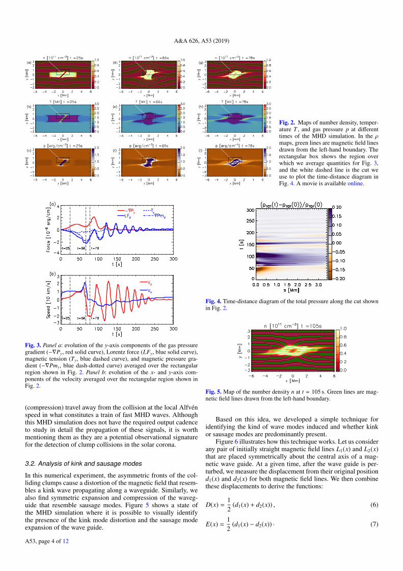
In this numerical experiment, the asymmetric fronts of the col-liding clumps cause a distortion of the magnetic field that resem-bles a kink wave propagating along a waveguide. Similarly, wealso find symmetric expansion and compression of the waveg-uide that resemble sausage modes. Figure 5 shows a state ofthe MHD simulation where it is possible to visually identifythe presence of the kink mode distortion and the sausage modeexpansion of the wave guide.

Fig. 4. Time-distance diagram of the total pressure along the cut shownin Fig. 2.

Fig. 5. Map of the number density n at t = 105 s. Green lines are mag-netic field lines drawn from the left-hand boundary.

Based on this idea, we developed a simple technique foridentifying the kind of wave modes induced and whether kinkor sausage modes are predominantly present.

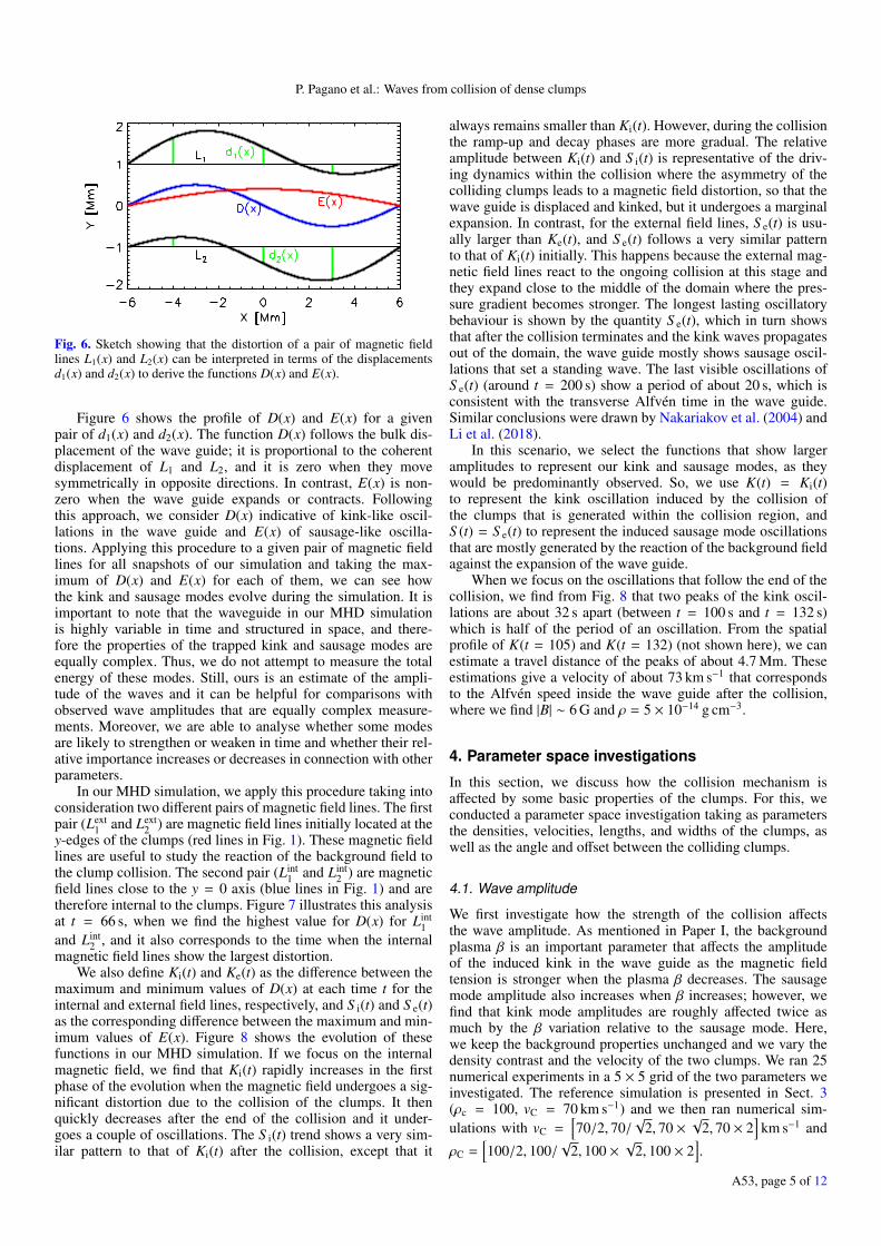
Figure 6 illustrates how this technique works. Let us considerany pair of initially straight magnetic field lines L1(x) and L2(x)that are placed symmetrically about the central axis of a mag-netic wave guide. At a given time, after the wave guide is per-turbed, we measure the displacement from their original positiond1(x) and d2(x) for both magnetic field lines. We then combinethese displacements to derive the functions:

D(x) =12

(d1(x) + d2(x)) , (6)

E(x) =12

(d1(x) − d2(x)) · (7)

A53, page 4 of 12

P. Pagano et al.: Waves from collision of dense clumps

Fig. 6. Sketch showing that the distortion of a pair of magnetic fieldlines L1(x) and L2(x) can be interpreted in terms of the displacementsd1(x) and d2(x) to derive the functions D(x) and E(x).

Figure 6 shows the profile of D(x) and E(x) for a givenpair of d1(x) and d2(x). The function D(x) follows the bulk dis-placement of the wave guide; it is proportional to the coherentdisplacement of L1 and L2, and it is zero when they movesymmetrically in opposite directions. In contrast, E(x) is non-zero when the wave guide expands or contracts. Followingthis approach, we consider D(x) indicative of kink-like oscil-lations in the wave guide and E(x) of sausage-like oscilla-tions. Applying this procedure to a given pair of magnetic fieldlines for all snapshots of our simulation and taking the max-imum of D(x) and E(x) for each of them, we can see howthe kink and sausage modes evolve during the simulation. It isimportant to note that the waveguide in our MHD simulationis highly variable in time and structured in space, and there-fore the properties of the trapped kink and sausage modes areequally complex. Thus, we do not attempt to measure the totalenergy of these modes. Still, ours is an estimate of the ampli-tude of the waves and it can be helpful for comparisons withobserved wave amplitudes that are equally complex measure-ments. Moreover, we are able to analyse whether some modesare likely to strengthen or weaken in time and whether their rel-ative importance increases or decreases in connection with otherparameters.

In our MHD simulation, we apply this procedure taking intoconsideration two different pairs of magnetic field lines. The firstpair (Lext

1 and Lext2 ) are magnetic field lines initially located at the

y-edges of the clumps (red lines in Fig. 1). These magnetic fieldlines are useful to study the reaction of the background field tothe clump collision. The second pair (Lint

1 and Lint2 ) are magnetic

field lines close to the y = 0 axis (blue lines in Fig. 1) and aretherefore internal to the clumps. Figure 7 illustrates this analysisat t = 66 s, when we find the highest value for D(x) for Lint

1and Lint

2 , and it also corresponds to the time when the internalmagnetic field lines show the largest distortion.

We also define Ki(t) and Ke(t) as the difference between themaximum and minimum values of D(x) at each time t for theinternal and external field lines, respectively, and S i(t) and S e(t)as the corresponding difference between the maximum and min-imum values of E(x). Figure 8 shows the evolution of thesefunctions in our MHD simulation. If we focus on the internalmagnetic field, we find that Ki(t) rapidly increases in the firstphase of the evolution when the magnetic field undergoes a sig-nificant distortion due to the collision of the clumps. It thenquickly decreases after the end of the collision and it under-goes a couple of oscillations. The S i(t) trend shows a very sim-ilar pattern to that of Ki(t) after the collision, except that it

always remains smaller than Ki(t). However, during the collisionthe ramp-up and decay phases are more gradual. The relativeamplitude between Ki(t) and S i(t) is representative of the driv-ing dynamics within the collision where the asymmetry of thecolliding clumps leads to a magnetic field distortion, so that thewave guide is displaced and kinked, but it undergoes a marginalexpansion. In contrast, for the external field lines, S e(t) is usu-ally larger than Ke(t), and S e(t) follows a very similar patternto that of Ki(t) initially. This happens because the external mag-netic field lines react to the ongoing collision at this stage andthey expand close to the middle of the domain where the pres-sure gradient becomes stronger. The longest lasting oscillatorybehaviour is shown by the quantity S e(t), which in turn showsthat after the collision terminates and the kink waves propagatesout of the domain, the wave guide mostly shows sausage oscil-lations that set a standing wave. The last visible oscillations ofS e(t) (around t = 200 s) show a period of about 20 s, which isconsistent with the transverse Alfvén time in the wave guide.Similar conclusions were drawn by Nakariakov et al. (2004) andLi et al. (2018).

In this scenario, we select the functions that show largeramplitudes to represent our kink and sausage modes, as theywould be predominantly observed. So, we use K(t) = Ki(t)to represent the kink oscillation induced by the collision ofthe clumps that is generated within the collision region, andS (t) = S e(t) to represent the induced sausage mode oscillationsthat are mostly generated by the reaction of the background fieldagainst the expansion of the wave guide.

When we focus on the oscillations that follow the end of thecollision, we find from Fig. 8 that two peaks of the kink oscil-lations are about 32 s apart (between t = 100 s and t = 132 s)which is half of the period of an oscillation. From the spatialprofile of K(t = 105) and K(t = 132) (not shown here), we canestimate a travel distance of the peaks of about 4.7 Mm. Theseestimations give a velocity of about 73 km s−1 that correspondsto the Alfvén speed inside the wave guide after the collision,where we find |B| ∼ 6 G and ρ = 5 × 10−14 g cm−3.

4. Parameter space investigations

In this section, we discuss how the collision mechanism isaffected by some basic properties of the clumps. For this, weconducted a parameter space investigation taking as parametersthe densities, velocities, lengths, and widths of the clumps, aswell as the angle and offset between the colliding clumps.

4.1. Wave amplitude

We first investigate how the strength of the collision affectsthe wave amplitude. As mentioned in Paper I, the backgroundplasma β is an important parameter that affects the amplitudeof the induced kink in the wave guide as the magnetic fieldtension is stronger when the plasma β decreases. The sausagemode amplitude also increases when β increases; however, wefind that kink mode amplitudes are roughly affected twice asmuch by the β variation relative to the sausage mode. Here,we keep the background properties unchanged and we vary thedensity contrast and the velocity of the two clumps. We ran 25numerical experiments in a 5 × 5 grid of the two parameters weinvestigated. The reference simulation is presented in Sect. 3(ρc = 100, vC = 70 km s−1) and we then ran numerical sim-ulations with vC =

[70/2, 70/

√2, 70 ×

√2, 70 × 2

]km s−1 and

ρC =[100/2, 100/

√2, 100 ×

√2, 100 × 2

].

A53, page 5 of 12

A&A 626, A53 (2019)

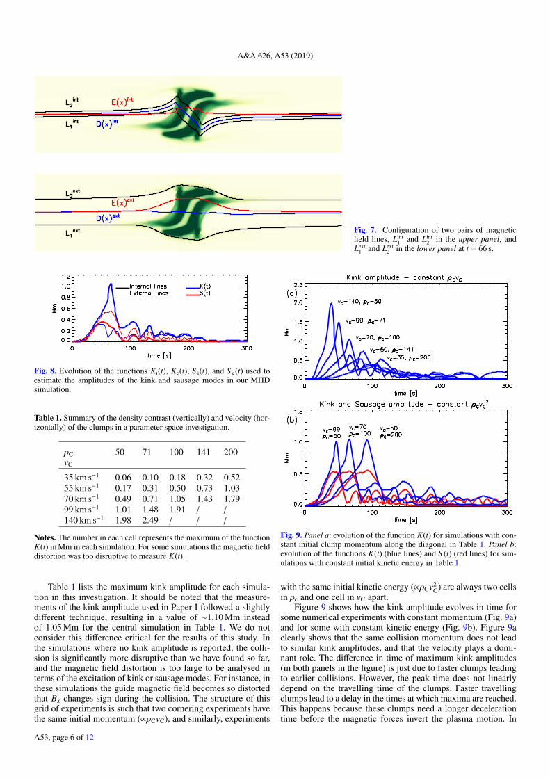
Fig. 7. Configuration of two pairs of magneticfield lines, Lint

1 and Lint2 in the upper panel, and

Lext1 and Lext

2 in the lower panel at t = 66 s.

Fig. 8. Evolution of the functions Ki(t), Ke(t), S i(t), and S e(t) used toestimate the amplitudes of the kink and sausage modes in our MHDsimulation.

Table 1. Summary of the density contrast (vertically) and velocity (hor-izontally) of the clumps in a parameter space investigation.

ρC 50 71 100 141 200vC

35 km s−1 0.06 0.10 0.18 0.32 0.5255 km s−1 0.17 0.31 0.50 0.73 1.0370 km s−1 0.49 0.71 1.05 1.43 1.7999 km s−1 1.01 1.48 1.91 / /

140 km s−1 1.98 2.49 / / /

Notes. The number in each cell represents the maximum of the functionK(t) in Mm in each simulation. For some simulations the magnetic fielddistortion was too disruptive to measure K(t).

Table 1 lists the maximum kink amplitude for each simula-tion in this investigation. It should be noted that the measure-ments of the kink amplitude used in Paper I followed a slightlydifferent technique, resulting in a value of ∼1.10 Mm insteadof 1.05 Mm for the central simulation in Table 1. We do notconsider this difference critical for the results of this study. Inthe simulations where no kink amplitude is reported, the colli-sion is significantly more disruptive than we have found so far,and the magnetic field distortion is too large to be analysed interms of the excitation of kink or sausage modes. For instance, inthese simulations the guide magnetic field becomes so distortedthat Bx changes sign during the collision. The structure of thisgrid of experiments is such that two cornering experiments havethe same initial momentum (∝ρCvC), and similarly, experiments

Fig. 9. Panel a: evolution of the function K(t) for simulations with con-stant initial clump momentum along the diagonal in Table 1. Panel b:evolution of the functions K(t) (blue lines) and S (t) (red lines) for sim-ulations with constant initial kinetic energy in Table 1.

with the same initial kinetic energy (∝ρCv2C) are always two cells

in ρc and one cell in vC apart.Figure 9 shows how the kink amplitude evolves in time for

some numerical experiments with constant momentum (Fig. 9a)and for some with constant kinetic energy (Fig. 9b). Figure 9aclearly shows that the same collision momentum does not leadto similar kink amplitudes, and that the velocity plays a domi-nant role. The difference in time of maximum kink amplitudes(in both panels in the figure) is just due to faster clumps leadingto earlier collisions. However, the peak time does not linearlydepend on the travelling time of the clumps. Faster travellingclumps lead to a delay in the times at which maxima are reached.This happens because these clumps need a longer decelerationtime before the magnetic forces invert the plasma motion. In

A53, page 6 of 12

P. Pagano et al.: Waves from collision of dense clumps

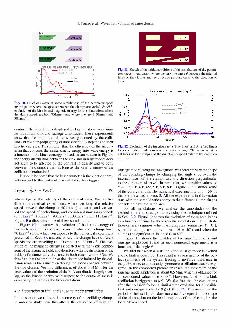
Fig. 10. Panel a: sketch of some simulations of the parameter spaceinvestigation where the speeds between the clumps are varied. Panel b:evolution of the kinetic and magnetic energy for the simulations wherethe clump speeds are both 70 km s−1 and where they are 110 km s−1 and30 km s−1.

contrast, the simulations displayed in Fig. 9b show very simi-lar maximum kink and sausage amplitudes. These experimentsshow that the amplitude of the waves generated by the colli-sions of counter-propagating clumps essentially depends on theirkinetic energies. This implies that the efficiency of the mecha-nism that converts the initial kinetic energy into wave energy isa function of the kinetic energy. Indeed, as can be seen in Fig. 9b,the energy distribution between the kink and sausage modes doesnot seem to be affected by the contrast in density and velocitybetween the clumps either, as long as the kinetic energy of thecollision is maintained.

It should be noted that the key parameter is the kinetic energywith respect to the centre of mass of the system EK(CM),

EK(CM) =12ρ (u − VCM)2 , (8)

where VCM is the velocity of the centre of mass. We ran fivedifferent numerical experiments where we keep the relativespeed between the clumps (140 km s−1) constant, and we var-ied the speed of each clump, and considered maximum speedsof 70 km s−1, 80 km s−1, 90 km s−1, 100 km s−1, and 110 km s−1.Figure 10a illustrates some of these simulations.

Figure 10b illustrates the evolution of the kinetic energy oftwo such numerical experiments: one in which both clumps have70 km s−1 (blue, which corresponds to the numerical experimentpresented in Sect. 3), and one where the clumps have differentspeeds and are travelling at 110 km s−1 and 30 km s−1. The evo-lution of the magnetic energy associated with the y-axis compo-nent of the magnetic field, and therefore with the distortion of thefield, is fundamentally the same in both cases (within 3%). Wethus find that the amplitude of the kink mode induced by the col-lision remains the same even though the speed changes betweenthe two clumps. We find differences of about 0.04 Mm for thepeak value and the evolution of the kink amplitudes largely over-lap, as the kinetic energy with respect to the centre of mass isessentially the same in the two simulations.

4.2. Repartition of kink and sausage mode amplitudes

In this section we address the geometry of the colliding clumpsin order to study how this affects the excitation of kink and

Fig. 11. Sketch of the initial conditions of the simulations of the param-eter space investigation where we vary the angle θ between the internalfaces of the clumps and the direction perpendicular to the direction oftravel.

Fig. 12. Evolution of the functions K(t) (blue lines) and S (t) (red lines)for some of the simulations where we vary the angle θ between the inter-nal faces of the clumps and the direction perpendicular to the directionof travel.

sausage modes along the waveguide. We therefore vary the shapeof the colliding clumps by changing the angle θ between theinternal faces of the clumps and the direction perpendicularto the direction of travel. In particular, we consider values ofθ = [0◦, 20◦, 40◦, 45◦, 50◦, 60◦, 80◦]. Figure 11 illustrates someof the configurations. The numerical experiment with θ = 50◦ isthe one presented in Sect. 3. All the experiments in this sectionstart with the same kinetic energy as the different clump shapesconsidered have the same area.

For all simulations, we analyse the amplitudes of theexcited kink and sausage modes using the technique outlinedin Sect. 3.2. Figure 12 shows the evolution of these amplitudesas a function of time for three specific simulations that illustratethree different regimes: when the clumps are symmetric (θ = 0◦),when the clumps are not symmetric (θ = 50◦), and when theclumps are significantly inclined (θ = 80◦).

Figure 13 shows the profiles of the maximum kink andsausage amplitudes found in each numerical experiment as afunction of the angle θ.

We find that when θ = 0◦, only the sausage mode is excitedand no kink is observed. This result is a consequence of the per-fect symmetry of the system leading to no force imbalance inthe y-direction, and thus only symmetric oscillations can be trig-gered. In the considered parameter space, the maximum of thesausage mode amplitude is about 0.5 Mm, which is obtained forall considered values of θ ≤ 60◦. However, for θ , 0 a kinkoscillation is triggered as well. We also find that the oscillationsafter the collision follow a similar time evolution for all visiblekink and sausage modes for θ ≤ 60 (Fig. 12). This means that theperiod of the oscillations does not crucially depend on the shapeof the clumps, but on the local properties of the plasma, i.e. thelocal Alfvén speed.

A53, page 7 of 12

A&A 626, A53 (2019)

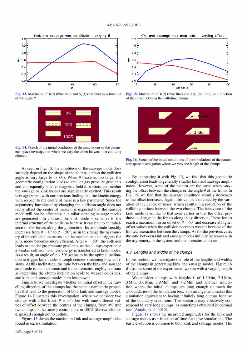
Fig. 13. Maximum of K(t) (blue line) and S e(t) (red line) as a functionof the angle θ.

Fig. 14. Sketch of the initial conditions of the simulations of the param-eter space investigation where we vary the offset between the collidingclumps.

As seen in Fig. 13, the amplitude of the sausage mode doesstrongly depend on the shape of the clumps, unless the collisionangle is very large (θ > 60). When θ becomes too large, thegeometric configuration leads to smaller gas pressure gradientsand consequently smaller magnetic field distortion, and neitherthe sausage or kink modes are significantly excited. This resultis in agreement with our previous finding that the kinetic energywith respect to the centre of mass is a key parameter. Since theasymmetry introduced by changing the collision angle does notreally affect the centre of mass, it is expected that the sausagemode will not be affected (i.e. similar standing sausage modesare generated). In contrast, the kink mode is sensitive to theinternal structure of the collision because it can lead to an imbal-ance of the forces along the y-direction. Its amplitude steadilyincreases from θ = 0◦ to θ = 50◦, as in this range the asymme-try of the collision increases and the mechanism that triggers thekink mode becomes more efficient. After θ = 50◦, the collisionleads to smaller gas pressure gradients, as the clumps experiencea weaker collision, and less energy is transferred to kink modes.As a result, an angle of θ ∼ 50◦ seems to be the optimal inclina-tion to trigger kink modes through counter-streaming flow colli-sions. At this inclination, the ratio between the kink and sausageamplitude is at a maximum and it then remains roughly constantas increasing the clump inclination leads to weaker collisions,and kink and sausage modes both lose power.

Similarly, we investigate whether an initial offset in the trav-elling direction of the clumps has the same asymmetric proper-ties that lead to the generation of both kink and sausage modes.Figure 14 illustrates this investigation, where we consider twoclumps with a flat front (θ = 0◦), but with nine different val-ues of offset between the centres of the clumps, from 0% (thetwo clumps on the same y coordinate), to 100% (the two clumpsdisplaced enough not to collide).

Figure 15 shows the maximum kink and sausage amplitudesfound in each simulation.

Fig. 15. Maximum of K(t) (blue line) and S (t) (red line) as a functionof the offset between the colliding clumps.

Fig. 16. Sketch of the initial conditions of the simulations of the param-eter space investigation where we vary the length of the clumps.

By comparing it with Fig. 13, we find that this geometricconfiguration leads to generally smaller kink and sausage ampli-tudes. However, some of the pattern are the same when vary-ing the offset between the clumps or the angle θ of the fronts InFig. 15, we find that the sausage amplitude steadily decreasesas the offset increases. Again, this can be explained by the vari-ation of the centre of mass, which results in a reduction of thecolliding surface between the two clumps. The behaviour of thekink mode is similar to that used earlier in that the offset pro-duces a change in the forces along the y-direction. These forcesreach a maximum for an offset of θ = 60◦ and decrease at higheroffset values when the collision becomes weaker because of thelimited interaction between the clumps. As for the previous case,the ratio between kink and sausage modes initially increases withthe asymmetry in the system and then remains constant.

4.3. Lengths and widths of the clumps

In this section, we investigate the role of the lengths and widthsof the clumps in generating kink and sausage modes. Figure 16illustrates some of the experiments we run with a varying lengthof the clumps.

We consider clumps with lengths L of 1.5 Mm, 2.4 Mm,3 Mm, 3.6 Mm, 3.9 Mm, and 4.2 Mm and another simula-tion where the initial clumps are long enough to touch thex-boundaries of the simulation box. This arrangement makes thissimulation equivalent to having infinitely long clumps becauseof the boundary conditions. This scenario may effectively cor-respond to very long clumps, as sometimes observed in coronalrain (Antolin et al. 2015).

Figure 17 shows the measured amplitudes for the kink andsausage modes as a function of time for these simulations. Thebasic evolution is common to both kink and sausage modes. The

A53, page 8 of 12

P. Pagano et al.: Waves from collision of dense clumps

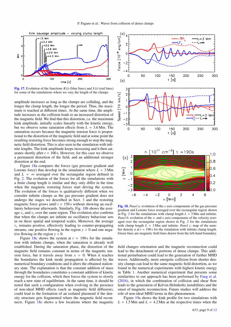
Fig. 17. Evolution of the functions K(t) (blue lines) and S (t) (red lines)for some of the simulations where we vary the length of the clumps.

amplitude increases as long as the clumps are colliding, and thelonger the clump length, the longer the period. Thus, the maxi-mum is reached at different times. At the same time, the ampli-tude increases as the collision leads to an increased distortion ofthe magnetic field. We find that this distortion, i.e. the maximumkink amplitude, initially scales linearly with the kinetic energy,but we observe some saturation effects from L = 3.6 Mm. Thesaturation occurs because the magnetic tension force is propor-tional to the distortion of the magnetic field and at some point theresulting restoring force becomes strong enough to stop the mag-netic field distortion. This is also seen in the simulation with infi-nite lengths. The kink amplitude keeps increasing and it then sat-urates shortly after t = 100 s. However, for this case we observea permanent distortion of the field, and an additional strongerdistortion at the end.

Figure 18a compares the forces (gas pressure gradient andLorentz force) that develop in the simulation where L = 3 Mmand L = ∞ averaged over the rectangular region defined inFig. 2. The evolution of the forces for all the simulations witha finite clump length is similar and they only differ in the timewhen the magnetic restoring forces start driving the system.The evolution of the forces is qualitatively different when weconsider infinite clumps as the gas pressure gradient does notundergo the stages we described in Sect. 3 and the restoringmagnetic force grows until t = 150 s without showing an oscil-latory behaviour afterwards. Similarly, Fig. 18b shows the aver-age vx and vy over the same region. This evolution also confirmsthat when the clumps are infinite no oscillatory behaviour setsin on these spatial and temporal scales. Moreover, the averagevx remains positive, effectively leading to counter-propagatingstreams, one positive flowing in the region y > 0 and one nega-tive flowing in the region y < 0.

Figure 18c shows the system at t = 190 s for the simula-tion with infinite clumps, when the saturation is already wellestablished. During the saturation phase, the distortion of themagnetic field remains constant in terms of the magnetic ten-sion force, but it travels away from x = 0. When it reachesthe boundaries the kink mode propagation is affected by thenumerical boundary conditions and it alters the obtained station-ary state. The explanation is that the constant addition of massthrough the boundaries constitutes a constant addition of kineticenergy for the collision, which then forces the system to slowlyreach a new state of equilibrium. At the same time, it should benoted that such a configuration when evolving in the presenceof non-ideal MHD effects (such as magnetic field diffusion),could lead to the formation of an isolated plasmoid if the den-sity structure gets fragmented where the magnetic field recon-nects. Figure 18c shows a few locations where the magnetic

Fig. 18. Panel a: evolution of the y-axis components of the gas pressuregradient and Lorentz force averaged over the rectangular region shownin Fig. 2 for the simulations with clump length L = 3 Mm and infinite.Panel b: evolution of the x- and y-axis components of the velocity aver-aged over the rectangular region shown in Fig. 2 for the simulationswith clump length L = 3 Mm and infinite. Panel c: map of the num-ber density n at t = 190 s for the simulation with infinite clump length.Green lines are magnetic field lines drawn from the left-hand boundary.

field changes orientation and the magnetic reconnection couldlead to the detachment of portions of dense clumps. This addi-tional perturbation could lead to the generation of further MHDwaves. Additionally, more energetic collision from shorter den-sity clumps can lead to the same magnetic field distortion, as wefound in the numerical experiments with highest kinetic energyin Table 1. Another numerical experiment that presents somesimilarities to our approach has been performed by Fang et al.(2016), in which the combination of collision and shear flowleads to the generation of Kelvin-Helmholtz instabilities and theonset of magnetic reconnection. Future studies will address therole of non-ideal MHD terms in this phenomenon.

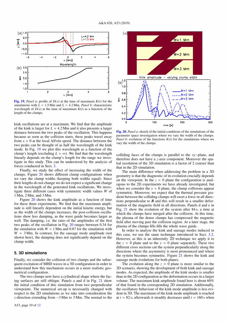
Figure 19a shows the kink profile for two simulations withL = 1.5 Mm and L = 4.2 Mm at the respective times when the

A53, page 9 of 12

A&A 626, A53 (2019)

Fig. 19. Panel a: profile of D(x) at the time of maximum K(t) for thesimulations with L = 1.5 Mm and L = 4.2 Mm. Panel b: characteristicwavelength of D(x) at the time of maximum K(t) as a function of thelength of the clumps.

kink oscillations are at a maximum. We find that the amplitudeof the kink is larger for L = 4.2 Mm and it also presents a largerdistance between the two peaks of the oscillation. This happensbecause as soon as the collision starts, these peaks travel awayfrom x = 0 at the local Alfvén speed. The distance between thetwo peaks can be thought of as half the wavelength of the kinkmode. In Fig. 19 we plot this wavelength as a function of theclump’s length (excluding L = ∞). We find that the wavelengthlinearly depends on the clump’s length for the range we inves-tigate in this study. This can be understood by the analysis offorces conducted in Sect. 3.

Finally, we study the effect of increasing the width of theclumps. Figure 20 shows different clump configurations whenwe vary the clump widths (keeping both widths equal). Sincetheir lengths do not change we do not expect a significant changein the wavelength of the generated kink oscillations. We inves-tigate three different cases with symmetric width values W of1 Mm, 2 Mm, and 3 Mm.

Figure 20 shows the kink amplitude as a function of timefor these three experiments. We find that the maximum ampli-tude is still linearly dependent on the initial kinetic energy, butas the width of the clumps increases, the post-collision oscilla-tions show less damping, as the wave guide becomes larger aswell. The damping, i.e. the ratio of the amplitudes of the firsttwo peaks of the oscillation in Fig. 20 ranges between 0.34 forthe simulation with W = 1 Mm and 0.87 for the simulation withW = 3 Mm. In contrast, for the sausage mode amplitude (notshown here), the damping does not significantly depend on theclump width.

5. 3D simulations

Finally, we consider the collision of two clumps and the subse-quent excitation of MHD waves in a 3D configuration in order tounderstand how this mechanism occurs in a more realistic geo-metrical configuration.

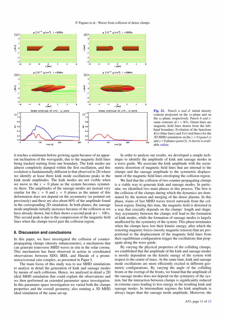
The two clumps now have a cylindrical shape where the fac-ing surfaces are still oblique. Panels a and d in Fig. 21 showthe initial condition of this simulation from two perpendicularviewpoints. The numerical set-up is necessarily changed withrespect to the 2D simulations as we take into consideration thez-direction extending from −3 Mm to 3 Mm. The normal to the

Fig. 20. Panel a: sketch of the initial conditions of the simulations of theparameter space investigation where we vary the width of the clumps.Panel b: evolution of the functions K(t) for the simulations where wevary the width of the clumps.

colliding faces of the clumps is parallel to the xy−plane, andtherefore does not have a z-axis component. Moreover the spa-tial resolution of the 3D simulation is a factor of 2 coarser thanthat in the 2D simulation.

The main difference when addressing the problem in a 3Dgeometry is that the diagnostic of its evolution crucially dependson the viewpoint. In the z = 0 plane the configuration is anal-ogous to the 2D experiments we have already investigated, butwhen we consider the y = 0 plane, the clump collisions appearsymmetric. Moreover, we expect that the thermal pressure gra-dient between the colliding clumps will exert a force in all direc-tions perpendicular to B and this will result in a smaller defor-mation of the magnetic field in all directions. Panels d and e inFig. 21 show the evolution of the system after 84 s, a time atwhich the clumps have merged after the collision. At this time,the plasma of the dense clumps has compressed the magneticfield after moving past the collision region. At a later stage, theplasma of the clumps fills fills the whole wave guide.

In order to analyse the kink and sausage modes induced inthis case, we use the same technique introduced in Sect. 3.2.However, as this is an inherently 2D technique we apply it tothe z = 0 plane and to the y = 0 plane separately. These twodifferent cross sections cut the system perpendicularly along thedirections where the asymmetry is most pronounced and wherethe system becomes symmetric. Figure 21 shows the kink andsausage mode evolutions for both planes.

The evolution along the z = 0 plane is more similar to the2D scenario, showing the development of both kink and sausagemodes. As expected, the amplitude of the kink modes is smallerthan in the 2D configuration as the deformation occurs in a largervolume. The maximum kink amplitude found here is about 60%of that found in the corresponding 2D simulation. Additionally,the oscillatory behaviour of the kink mode amplitude is less evi-dent in 3D. The maximum of the kink mode amplitude is reachedat t = 82 s; afterwards it steadily decreases until t = 160 s when

A53, page 10 of 12

P. Pagano et al.: Waves from collision of dense clumps

Fig. 21. Panels a and d: initial densitycontour projected on the xy-plane and onthe xz-plane, respectively. Panels b and e:same contours at t = 84 s. Green lines aremagnetic field lines drawn from the left-hand boundary. Evolution of the functionsK(t) (blue lines) and S (t) (red lines) for the3D MHD simulation on the z = 0 (panel c)and y = 0 planes (panel f). A movie is avail-able online.

it reaches a minimum before growing again because of an appar-ent inclination of the waveguide, due to the magnetic field linesbeing tracked starting from one boundary. The kink modes arealmost completely damped within the first oscillation, and thisevolution is fundamentally different to that observed in 2D wherewe identify at lease three kink mode oscillations peaks in thekink mode amplitudes. The kink modes are not visible whenwe move to the y = 0 plane as the system becomes symmet-ric there. The amplitudes of the sausage modes are instead verysimilar for the z = 0 and y = 0 planes as the nature of thisdeformation does not depend on the asymmetry (as pointed outpreviously) and these are also about 60% of the amplitude foundin the corresponding 2D simulation. In both planes, the sausagemode amplitude initially increases because of the collision as wehave already shown, but it then shows a second peak at t ∼ 100 s.This second peak is due to the compression of the magnetic fieldlines when the clumps travel past the collision region.

6. Discussion and conclusions

In this paper, we have investigated the collision of counter-propagating clumps (density enhancements), a mechanism thatcan generate transverse MHD waves in situ in the solar corona.This mechanism has been observed in action in coordinatedobservations between SDO, IRIS, and Hinode of a promi-nence/coronal rain complex, as presented in Paper I.

The main focus of this study was to use MHD simulationsto analyse in detail the generation of kink and sausage modesby means of such collisions. Hence, we analysed in detail a 2Dideal MHD simulation that could explain the observations andwe then performed an extended parameter space investigation.In this paramater space investigation we varied both the clumpsproperties and the overall geometry, also running a 3D MHDideal simulation of the same set-up.

In order to analyse our results, we developed a simple tech-nique to identify the amplitude of kink and sausage modes ina wave guide. We associate the kink amplitude with the asym-metric distortion of magnetic field lines that are internal to theclumps and the sausage amplitude to the symmetric displace-ment of the magnetic field lines enveloping the collision region.

We find that the collision of two counter-propagating clumpsis a viable way to generate kink and sausage modes. In partic-ular, we identified two main phases in this process. The first isthe collision of the clumps during which the dynamics are dom-inated by the motion and merging of the dense plasma. In thisphase, trains of fast MHD waves travel outwards from the col-lision region. During this time, the magnetic field is distorted ina way that crucially depends on the clumps’ length and shape.Any asymmetry between the clumps will lead to the formationof kink modes, while the formation of sausage modes is largelyunaffected by the symmetry of the system. This phase terminateswhen the clumps have lost their kinetic energy, after which therestoring magnetic forces (mostly magnetic tension) that are pro-portional to the displacement of the magnetic field lines fromtheir equilibrium configuration trigger the oscillations that prop-agate along the wave guide.

By varying the physical properties of the colliding clumps,we established that the amplitude of the kink and sausage modesis mostly dependent on the kinetic energy of the system withrespect to the centre of mass. At the same time, kink and sausagemode oscillations are more efficiently excited in different geo-metric configurations. By varying the angle of the collidingfronts or the overlap of the fronts, we found that the amplitude ofthe sausage modes does not depend on the symmetry of the sys-tem, but the interaction between clumps is significantly reducedin extreme cases leading to less energy in the resulting kink andsausage modes. In intermediate regimes the kink amplitude isalways larger than the sausage mode amplitude. Moreover, the

A53, page 11 of 12

A&A 626, A53 (2019)

amplitude of the kink modes increases linearly with the clump’slength because of the associated kinetic energy. However, verylong clumps can reach a saturation regime. This occurs when therestoring magnetic forces due to the deformation of the magneticfield become equal to the thermal pressure gradient driven bythe collision. The initial wavelength of the kink modes increaseswith the length of the clumps. The generated kink modes propa-gate away from the collision, while the generated sausage modesbecome standing due to the symmetry in the longitudinal forces.Finally, we found that while the initial kink amplitude is propor-tional to the kinetic energy, less damping is obtained for largerclump widths in our model.

In order to better relate with a realistic scenario, we extendedour analysis to a fully 3D configuration where the clumps arecylindrical. The key differences are first that the kink amplitudeis nearly halved because the magnetic field line distortion occurson the volume around the cylinders and that the observed modeamplitudes and the apparent asymmetry of the system cruciallydepend on the viewpoint. However, only through forward mod-elling can this effect be properly estimated.

In conclusion, this work has improved our understandingof the mechanism behind the generation of MHD waves in thesolar corona due to the collision of counter-propagating plasmaclumps. At the same time, more work is required in order to linkthis model with observations, and future efforts will focus onforward modelling more realistic numerical models for propercomparison with observations

Acknowledgements. This research has received funding from the UK Scienceand Technology Facilities Council (Consolidated Grant ST/K000950/1) and theEuropean Union Horizon 2020 research and innovation programme (grant agree-ment No. 647214). P.A. acknowledges funding from the STFC Ernest RutherfordFellowship (No. ST/R004285/1). This research was supported by the ResearchCouncil of Norway through its Centres of Excellence scheme, project number262622. This work used the DiRAC@Durham facility managed by the Insti-tute for Computational Cosmology on behalf of the STFC DiRAC HPC Facility

(www.dirac.ac.uk). The equipment was funded by BEIS capital funding viaSTFC capital grants ST/P002293/1, ST/R002371/1, and ST/S002502/1, DurhamUniversity, and STFC operations grant ST/R000832/1. DiRAC is part of theNational e-Infrastructure. We acknowledge the use of the open source (gitori-ous.org/amrvac) MPI-AMRVAC software, relying on coding efforts from C. Xia,O. Porth, and R. Keppens.

ReferencesAlexander, C. E., Walsh, R. W., Régnier, S., et al. 2013, ApJ, 775, L32Antolin, P., & Rouppe van der Voort, L. 2012, ApJ, 745, 152Antolin, P., Okamoto, T. J., De Pontieu, B., et al. 2015, ApJ, 809, 72Antolin, P., Pagano, P., De Moortel, I., & Nakariakov, V. M. 2018, ApJ, 861,

L15Arregui, I. 2015, Trans. R. Soc. London Ser. A, 373, 20140261Brosius, J. W. 2013, ApJ, 762, 133Brosius, J. W., & Phillips, K. J. H. 2004, ApJ, 613, 580Chitta, L. P., Jain, R., Kariyappa, R., & Jefferies, S. M. 2012, ApJ, 744, 98De Moortel, I., & Nakariakov, V. M. 2012, Trans. R. Soc. London Ser. A, 370,

3193De Pontieu, B., Title, A. M., Lemen, J. R., et al. 2014, Sol. Phys., 289, 2733Fang, X., Yuan, D., Xia, C., Van Doorsselaere, T., & Keppens, R. 2016, ApJ,

833, 36Gupta, G. R., Sarkar, A., & Tripathi, D. 2018, ApJ, 857, 137Kleint, L., Antolin, P., Tian, H., et al. 2014, ApJ, 789, L42Kohutova, P., & Verwichte, E. 2017, A&A, 606, A120Kohutova, P., & Verwichte, E. 2018, A&A, 613, L3Kosugi, T., Matsuzaki, K., Sakao, T., et al. 2007, Sol. Phys., 243, 3Krishna Prasad, S., Jess, D. B., & Khomenko, E. 2015, ApJ, 812, L15Li, B., Guo, M.-Z., Yu, H., & Chen, S.-X. 2018, ApJ, 855, 53Matsumoto, T., & Kitai, R. 2010, ApJ, 716, L19Morton, R. J., Weberg, M. J., & McLaughlin, J. A. 2019, Nat. Astron., 3, 223Nakariakov, V. M., Arber, T. D., Ault, C. E., et al. 2004, MNRAS, 349, 705Oliver, R., Soler, R., Terradas, J., & Zaqarashvili, T. V. 2016, ApJ, 818, 128Pesnell, W. D., Thompson, B. J., & Chamberlin, P. C. 2012, Sol. Phys., 275, 3Porth, O., Xia, C., Hendrix, T., Moschou, S. P., & Keppens, R. 2014, ApJS, 214,

4Reale, F. 2010, Sol. Phys., 7, 5Verwichte, E., & Kohutova, P. 2017, A&A, 601, L2Verwichte, E., Antolin, P., Rowlands, G., Kohutova, P., & Neukirch, T. 2017,

A&A, 598, A57

A53, page 12 of 12