mglTEX v4.2 usage sample

Diego Sejas Viscarra Alexey Balakin

July 9, 2016

Abstract

mglTEX is a LATEX package that allows the creation of graphics directlyfrom MGL scripts of the MathGL library (by Alexey Balakin) inside docu-ments. The MGL code is extracted, executed (if shell escape is activated),and the resulting graphics are automatically included.

This document is intended as a sample of the capabilities of mglTEX,as well as a brief introduction to the package, for those who want to startright away to use it, without diving into the a little bit more technicaldocumentation.

1 Basics on environments

mgl The easiest way to embed MGL code is the mgl environment. It extractsits contents to a main script associated to the document.1 If shell es-cape is activated, LATEX will take care of calling mglconv (the MathGLcompiler) with the appropriate settings, and the resulting image will beautomatically included.

For example, you could write:

\begin{figure}[!ht]

\centering

\begin{mgl}[width=0.95\textwidth,height=6cm]

call ’prepare1d’

subplot 2 1 0 ’<_’ : title ’Standard data plot’

box : axis : grid ’xy’ ’;k’

plot y rGb

subplot 2 1 1 ’<_’ : title ’Region plot’

ranges -1 1 -1 1 : origin 0 0

new y1 200 ’x^3-x’ : new y2 200 ’x’

axis : grid ’xy’ ’W’

region y1 y2 ’ry’

1Generally, the main script has the same name as the document being compiled. In orderto rename it or create a new one, the \mglname command can be used.

1

plot y1 ’2k’ : plot y2 ’2k’

text -0.75 -0.35 ’\i{A}_1’ ’k’ : text 0.75 0.25 ’\i{A}_2’ ’k’

\end{mgl}

caption{A simple plot created by \mglTeX’s \texttt{mgl} environment}

\end{figure}

This will produce the following image:

Figure 1: A simple plot create by mglTEX’s mgl environment

Two important aspects of mglTEX can be noted from this example: First,the mgl environment accepts the same optional argument as the \includegraphicscommand from the graphicx package. Actually, it also accepts other op-tional arguments, called gray (to activate/deactivate gray-scale mode),mglscale (to set the factor for scaling the image file), quality (to setthe quality of the image), variant (to chose the variant of the argumentsof MGL commands in the script), imgext (to specify the extension ofthe resulting graphic file), and label (to specify a name to save the im-age). Most of these options are available to every mglTEX environment orcommand to create graphics.

The second aspect to be noted about the example is that this script callsa MGL function, prepare1d, which hasn’t been defined yet. mglTEXprovides the mglfunc environment for this purpose (see below).

mglfunc This environment can be used in any part of the LATEX document;mglTEX takes care of placing the corresponding code at the end of themain script, as has to be done in the MGL language.

For example, the function prepare1d that is called in the script above isdefined like this

\begin{mglfunc}{prepare1d}

2

new y 50 3

modify y ’0.7*sin(2*pi*x)+0.5*cos(3*pi*x)+0.2*sin(pi*x)’

modify y ’sin(2*pi*x)’ 1

modify y ’cos(2*pi*x)’ 2

\end{mglfunc}

As you can see, only the body of the function has to be written. The num-ber of arguments of the function can be passed to mglfunc as optional ar-gument, like in the code \begin{mglfunc}[3]{func_with_three_args}.

mgladdon This environment just adds its contents to the main script, with-out producing any image. It is useful to load dynamic libraries, defineconstants, etc.

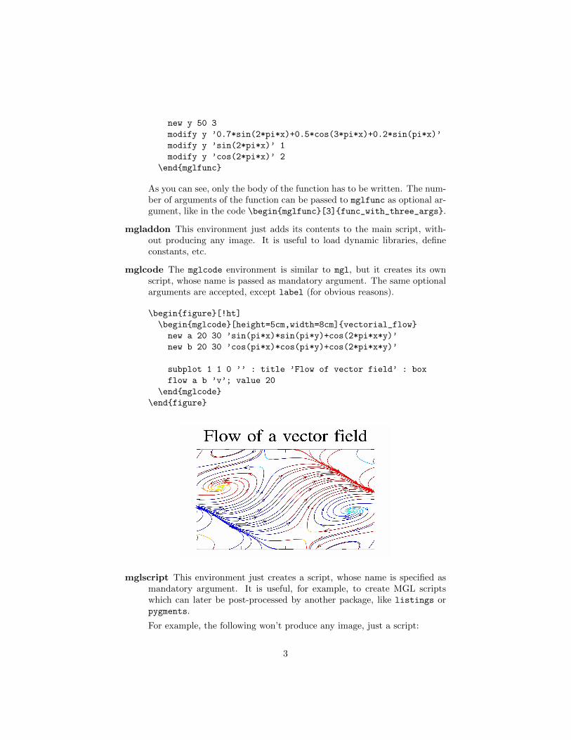
mglcode The mglcode environment is similar to mgl, but it creates its ownscript, whose name is passed as mandatory argument. The same optionalarguments are accepted, except label (for obvious reasons).

\begin{figure}[!ht]

\begin{mglcode}[height=5cm,width=8cm]{vectorial_flow}

new a 20 30 ’sin(pi*x)*sin(pi*y)+cos(2*pi*x*y)’

new b 20 30 ’cos(pi*x)*cos(pi*y)+cos(2*pi*x*y)’

subplot 1 1 0 ’’ : title ’Flow of vector field’ : box

flow a b ’v’; value 20

\end{mglcode}

\end{figure}

mglscript This environment just creates a script, whose name is specified asmandatory argument. It is useful, for example, to create MGL scriptswhich can later be post-processed by another package, like listings orpygments.

For example, the following won’t produce any image, just a script:

3

\begin{mglscript}{Gaston_Neiza}

clf ’k’

attachlight on

subplot 1 1 0 ’’ : title ’Gaston\utf0x0027{}s Surface’

ranges -13 13 -40 40

new a 200 200 ’-x+(2*0.84*cosh(0.4*x)*sinh(0.4*x))/(0.4*((sqrt(0.84)*cosh(0.4*x))^2+(0.4*sin(sqrt(0.84)*y))))+0.5*sin(pi/2*x)’

new b 200 200 ’(2*sqrt(0.84)*cosh(0.45*x)*(-(sqrt(0.84)*sin(y)*cos(sqrt(0.84)*y))+cos(y)*sin(sqrt(0.84)*y)))/(0.4*((sqrt(0.84)*cosh(0.4*x))^2+2*(0.4*sin(sqrt(0.84)*x))^2))’

new c 200 200 ’(2*sqrt(0.84)*cosh(0.45*x)*(-(sqrt(0.84)*cos(y)*cos(sqrt(0.84)*y))-sin(y)*sin(sqrt(0.84)*y)))/(0.4*((sqrt(0.84)*cosh(0.4*x))^2+2*(0.4*sin(sqrt(0.84)*x))^2))’

rotate 60 60

light on : light 0 1 1 0

xrange c : yrange b : zrange a : crange c

surf c b a ’#’; meshnum 100

subplot 2 1 1 ’’

title ’Neiza\utf0x0027{}s Rose’

ranges -13 13 -40 40

new a 700 700 ’-x+(1.5*cos(x^2))/(0.4*((sqrt(0.84)*cosh(0.4*x))^2+(0.4*sin(sqrt(0.84)*y))))+0.5*cos(pi/2*x)’

new b 700 700 ’(sqrt(0.5)*cos(0.25*x)*((sqrt(0.84)*sin(y)*cos(0.75*y))+cos(y)*sin(sqrt(0.84)*y)))/(0.4*((sqrt(0.84)*cosh(0.4*x))^2+2*(0.4*sin(sqrt(0.84)*x))^2))’

new c 700 700 ’(sqrt(0.5)*cos(0.25*x)*((sqrt(0.84)*cos(y)*sin(0.75*y))-sin(y)*sin(sqrt(0.84)*y)))/(0.4*((sqrt(0.84)*cosh(0.4*x))^2+2*(0.4*sin(sqrt(0.84)*x))^2))’

rotate 75 130

light on : light 0 0 0 1 ’w’ 0.5 : light 1 -1 0 0 ’r’ 0.85 : light 2 -1 0 0 ’w’ 0.75

xrange c : yrange b : zrange a : crange c

surf c b a ’r’

\end{mglscript}

mglblock It writes its contents verbatim to a file, specified as mandatory ar-gument, and to the LATEX document.

For example:

\begin{mglblock}{fractal}

list A [0,0,0,.16,0,0,.01] [.85,.04,-.04,.85,0,1.6,.85] [.2,-.26,.23,.22,0,1.6,.07] [-.15,.28,.26,.24,0,.44,.07]

ifs2d f A 100000

subplot 2 1 0 ’<_’ : title ’A fractal fern’

ranges f(0) f(1) : axis

plot f(0) f(1) ’G#o ’; size 0.05

subplot 2 1 1 ’<_’ : title ’Bifurcation plot’

ranges 0 4 0 1 : axis

bifurcation 0.005 ’x*y*(1-y)’ ’R’

\end{mglblock}

fractal.mgl

1. list A [0,0,0,.16,0,0,.01] [.85,.04,-.04,.85,0,1.6,.85]

[.2,-.26,.23,.22,0,1.6,.07]

[-.15,.28,.26,.24,0,.44,.07]

4

2. ifs2d f A 100000

3. subplot 2 1 0 ’<_’: title ’A fractal fern’

4. ranges f(0) f(1) : axis

5. plot f(0) f(1) ’G#o ’; size 0.05

6.

7. subplot 2 1 1 ’<_’: title ’Bifurcation plot’

8. ranges 0 4 0 1 : axis

9. bifurcation 0.005 ’x*y*(1-y)’’R’

As you can see, although this is a verbatim-like environment, very longlines of code are split to fit the paragraph. Each line of code is numbered,this can be disabled with the lineno option, like \begin{mglblock}[lineno=false]{fractal}.

mglverbatim This is like mglblock environment, but it doesn’t produce anyscript, just typesets the code to the LATEX document. It accepts thelineno option, plus the label option, in case you want to associate aname to the code.

mglcomment This environment is used to embed comments in the document.You can control whether the contents of this environment are displayedor not, using the comments and nocomments package options, or the\mglcomments{on} and mglcomments{off} commands.

An example of this would be:

\begin{mglcomments}

This comment will be shown because we used the "comments" package option for mglTeX

\end{mglcomments}

< - - - - - - - - - - - - - - - mglTEX comment - - - - - - - - - - - - - - - >

This comment will be shown because we used the

"comments" package option for mglTeX

< - - - - - - - - - - - - - - - mglTEX comment - - - - - - - - - - - - - - - >

Once again, long lines are broke down to fit the paragraph.

2 Basics on commands

\mglgraphics This command takes the name of an external MGL script, com-piles it, and includes the resulting image. It accespt the same optionalarguments as the mgl environment, except for label, plus a path option,which can be used to specify the location of the script. This is useful whenyou have a script outside of the LATEX document (sent by a colleague forexample), but you don’t want to transcript it to your document.

5

For example, in order to display the image of the script we created withmglscript environment, we write:

\begin{figure}[!ht]

\centering

\mglgraphics[height=9cm,width=18cm]{Gaston_Neiza}

\caption{‘‘Gaston’s Surface’’ and ‘‘Neiza’s Rose’’ are named after Diego Sejas’ parents}

\end{figure}

Figure 2: “Gaston’s Surface” and “Neiza’s Rose” are named after Diego Sejas’parents

We could also could compile the script we created with the mglblock

environment:

\begin{figure}[!ht]

\centering

\mglgraphics[height=7cm,width=10cm]{fractal}

\caption{Examples of fractal behavior}

\end{figure}

\mglinclude This is equivalent to the mglblock environment, but works forexternal scripts.

\mglplot This command allows the fast creation of plots. It takes one manda-tory argument, which is a block of MGL code to produce the plot. Accepts

6

Figure 3: Examples of fractal behavior

the same optional arguments as the mgl environment, plus an additionalone, setup, that can be used to specify a block of code to append, definedinside a mglsetup environment (see the example below).

The mglsetup environment can be used if many plots will have the samesettings (background color, etc.). Instead of writing the same code overand over again, it can be introduced in that environment, and used withthe \mglplot command.

An example of use of the mglsetup environment and the \mglplot com-mand would be:

\begin{mglsetup}{3d}

clf ’W’

rotate 50 60

light on

box : axis : grid ’xyz’ ’;k’

\end{mglsetup}

\begin{figure}[!ht]

\centering

\mglplot[setup=3d,height=5cm,width=8cm]{fsurf ’cos(4*pi*hypot(x,y))*exp(-abs(x+y))’}

\end{figure}

\begin{figure}[!ht]

\centering

\mglplot[setup=3d,height=5cm,width=8cm]{fsurf ’sin(pi*(x+y))’}

\end{figure}

7

There are more environments and commands defined by mglTEX. The onespresented here are the most basic. More on this topic can be found in thedocumentation.

8