Metrics, Algorithms & Follow-ups

• Profile Similarity Measures• Cluster combination procedures • Hierarchical vs. Non-hierarchical Clustering• Statistical follow-up analyses

•“Internal” ANOVA & ldf Analyses•“External” ldf ANOVA & ldf Analyses

Profile Dissimilarity Measures• For each formula

• y are data from 1st person & x are data from 2nd person being compared• summing across vars

• Euclidean [ (y - x)² ]

• Squared Euclidean (y - x)² (probably most popular)

• City-Block | y - x |

• Chebychev max | y - x |

• Cosine cos rxy (similarity index)

Euclidean [ (y - x)² ]

-3 -2 -1 0 1 2 3 V1

-3 -

2 -

1 0

1

2

3

V2

( 42 + 22) = 20 = 4.47

X = 2, 0

4.47 represents the “multivariate dissimilarity” of X & Y

Y = -2, -2

[-2 – 0]2 ([-2 – 2]2 + )

Squared Euclidean (y - x)²

-3 -2 -1 0 1 2 3 V1-3

-2

-1

0

1

2

3 V

2 ( 42 + 22) = 20

X = 2, 0

20 represents the “multivariate dissimilarity” of X & Y

Squared Euclidean is a little better at “noticing” strays• remember that we use a square root transform to “pull in” outliers• leaving the value squared makes the strays stand out a bit more

Y = -2, -2

[-2 – 0]2 ([-2 – 2]2 + )

City Block |y – x|

-3 -2 -1 0 1 2 3 V1-3

-2

-1

0

1

2

3 V

2

( 4 + 2) = 6

X = 2, 0

Y = -2, -2

[-2 – 0] ([-2 – 2] + )

So named because in a city you have to go “around the block” you can’t “cut the diagonal”

-3 -2 -1 0 1 2 3 V1

-3 -

2 -

1 0

1

2

3

V2

max ( 4 & 2) = 4

X = 2, 0

Y = -2, -2

| -2 – 0 | = 2

| -2 – 2 | = 4

Uses the “greatest univariate difference” to represent the multivariate dissimilarity.

Chebychev max | y - x |

-3 -2 -1 0 1 2 3 V1

-3 -

2 -

1 0

1

2

3

V2

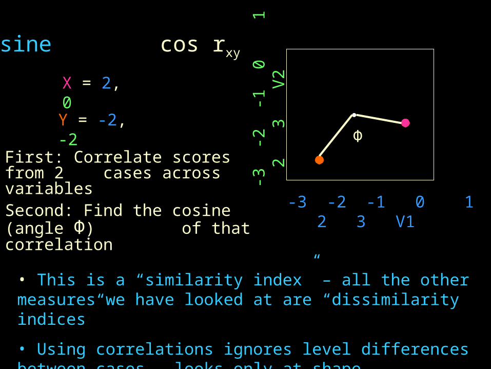
• This is a “similarity index” – all the other measures we have looked at are “dissimilarity indices”

• Using correlations ignores level differences between cases – looks only at shape differences (see next page)

Cosine cos rxy

X = 2, 0

Y = -2, -2Φ

Second: Find the cosine (angle Φ) of that correlation

First: Correlate scores from 2 cases across variables

A B C D E

Based on Euclidean or Squared Euclidean these four cases would probably group as:

• orange & blue

• green & yellow

While those within the groups have somewhat different shapes, they are very similar levels

Based on Cos r these four cases would probably group as:

• blue & green

• orange & yellow

Because correlation pays attention only to profile shape

It is important to carefully consider how you want to define “profile similarity” when clustering – it will likely change the results you get.

How Hierarchical Clustering works

• Data in an “X” matrix (cases x variables)

• Compute the “profile similarity” of all pairs of cases and put

those values in a “D” matrix (cases x cases)

• Start with # clusters = # cases (1 case in @ cluster)

• On each step• Identify the 2 clusters that are “most similar”

• A “cluster” may have 1 or more cases• Combine those 2 into a single cluster

• Re-compute the “profile similarity” among all cluster pairs

• Repeat until there is a single cluster

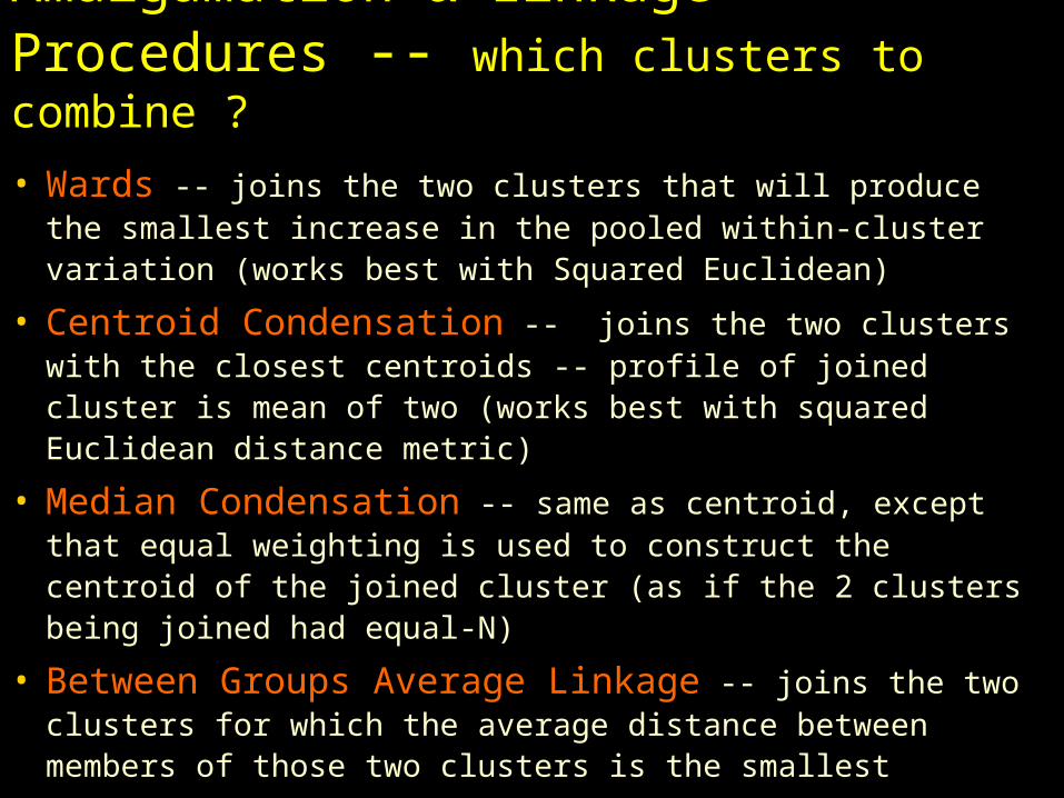
Amalgamation & Linkage Procedures -- which clusters to combine ?

• Wards -- joins the two clusters that will produce the smallest increase in the pooled within-cluster variation (works best with Squared Euclidean)

• Centroid Condensation -- joins the two clusters with the closest centroids -- profile of joined cluster is mean of two (works best with squared Euclidean distance metric)

• Median Condensation -- same as centroid, except that equal weighting is used to construct the centroid of the joined cluster (as if the 2 clusters being joined had equal-N)

• Between Groups Average Linkage -- joins the two clusters for which the average distance between members of those two clusters is the smallest

Amalgamation & Linkage Procedures, cont.

• Within-groups Average Linkage -- joins the two clusters for which the average distance between members of the resulting cluster will be smallest

• Single Linkage -- two clusters are joined which have the most similar two cases

• Complete Linkage -- two clusters are joined for which the maximum distance between a pair of cases in the two clusters is the smallest

Wards -- joins the two clusters that will produce the smallest increase in the pooled within-cluster variation

• works well with Squared Euclidean metrics (identifies strays)• attempts to reduce cluster overlay by minimizing SSerror • produces more clusters, each with lower variability

Computationally intensive, but Statistically simple …

On each step …

1. Take every pair of clusters & combine them

• Compute the variance across cases for each variable

• Combine those univariate variances into a multivariate variance index

2. Identify the pair of clusters with the smallest multivariate variance index

3. Those two clusters are combined

Centroid Condensation-- joins the two clusters with the closest centroids -- profile of joined cluster is mean of two

The distance between every pair of cluster centroids is computed.

The two clusters with the shortest centroid distance are joined

The centroid for the new cluster is computed as the mean of the joined centroids

Compute the centroid for each cluster

• new centroid will be closest to the larger group – it contributesmore cases

• if a “stray” is added, it is unlikely to mis-position the new centroid

Median Condensation-- joins the two clusters with the closest centroids -- profile of joined cluster is median of two -- is better than last if suspect groups of different size

The distance between every pair of cluster centroids is computed.

The two clusters with the shortest centroid distance are joined

The centroid for the new cluster is computed as the median of the joined centroids

Compute the centroid for each cluster

• new centroid will be closest to the larger group – it contributesmore cases

• if a “stray” is added, it is very likely to mis-position new centroid

Between Groups Average Linkage-- joins the two clusters with smallest average cross-linkage -- profile of joined cluster is mean of two

For each pair of clusters find the links across the clusters – links for one shown– yep, there are lots of these

The two clusters with the shortest average centroid distance are joined-- more complete than just comparing centroid distances

The centroid for the new cluster is computed as the mean of the joined centroids

• new centroid will be closest to the larger group – it contributesmore cases

• if a “stray” is added, it is unlikely to mis-position the new centroid

Within Groups Average Linkage-- joins the two clusters with smallest average within linkage -- profile of joined cluster is mean of two

For each pair of clusters find the links within that cluster pair – a few between & within shown– yep, there are scads of these

The two clusters with the shortest average centroid distance are joined-- more complete than between groups average linkage

The centroid for the new cluster is computed as the mean of the joined centroids

• like Wards, but w/ “smallest distance” instead of “minimum SS”• new centroid will be closest to the larger group • if a “stray” is added, it is unlikely to mis-position the new centroid

Single Linkage-- joins the two clusters with the nearest neighbors -- profile of joined cluster is computed from case data

The two clusters with the shortest nearest neighbor distance are joined

The centroid for the new cluster is computed from all cases in the new cluster

Compute the nearest neighbor distance for each cluster pair

• groupings based on position of a single pair of cases • outlying cases can lead to “undisciplined groupings” – see above

Complete Linkage-- joins the two clusters with the nearest farthest neighbors -- profile of joined cluster is computed from case data

The two clusters with the shortest farthest neighbor distance are joined

The centroid for the new cluster is computed from all cases in the new cluster

Compute the farthest neighbor distance for each cluster pair

• groupings based on position of a single pair of cases • can lead to “undisciplined groupings” see above

k-means Clustering – Non-hierarchical• select the desired number of clusters• identify the “k” clustering variablesFirst Iteration• the computer places each case into the k-dimensional space

• the computer randomly assigns cases to the “k” groups &computes the k-dim centroid of each group• compute the distance from each case to each group centroid • cases are re-assigned to the group to which they are closestSubsequent Iterations• re-compute the centroid for each group• for each case re-compute the distance to each group centroid• cases are re-assigned to the group to which they are closestStop• when cases don’t change groups or centroids don’t change• failure to converge can happen, but doesn’t often

Hierarchical “&” k-means Clustering There are two major issues in cluster analysis…leading to a third1. How many clusters are there ?2. Who belongs to each cluster ?

3. What are the clusters ? That is, how do we describe them, based on a description of who is in each ??

• Different combinations of clustering metrics, amalgamation and link often lead to different answers to these questions.

• Hierarchical & K-means clustering often lead to different answers as well.

• The more clusters in the solutions derived by different procedures, the more likely those clusters are to disagree

• How different procedures handle strays and small-frequencyprofiles often accounts for the resulting differences

Using ldf when clustering• It is common to hear that following a clustering with an ldf is “silly” -- depends !• There are two different kinds of ldfs -- with different goals . . .

• predicting groups using the same variables used to create the clusters an “internal ldf”

• always “works” -- there are discriminable groups (duh!!)• but will learn something from what variables separate which groups (may be

a small subset of the variables used)

• Reclassification errors tell you about “strays” & “forces”• gives you a “spatial model” of the clusters (concentrated vs. diffuse

structure, etc.)

• predicting groups using a different set of variables than those used to create the clusters an “external ldf”

• asks if knowing group membership “tells you anything”