methods to detect, characterize, and remove motion ...cogns.northwestern.edu/cbmg/motion in resting...

NeuroImage 84 (2014) 320–341

Contents lists available at ScienceDirect

NeuroImage

j ourna l homepage: www.e lsev ie r .com/ locate /yn img

Methods to detect, characterize, and remove motion artifact in restingstate fMRI

Jonathan D. Power a,⁎, Anish Mitra a, Timothy O. Laumann a, Abraham Z. Snyder a,b,Bradley L. Schlaggar a,b,c,d, Steven E. Petersen a,b,d,e,f,g

a Dept. of Neurology, Washington University School of Medicine in St. Louis, 660 S. Euclid Ave., St. Louis, MO 63110, USAb Dept. of Radiology, Washington University School of Medicine in St. Louis, 660 S. Euclid Ave., St. Louis, MO 63110, USAc Dept. of Pediatrics, Washington University School of Medicine in St. Louis, 660 S. Euclid Ave., St. Louis, MO 63110, USAd Dept. of Anatomy & Neurobiology, Washington University School of Medicine in St. Louis, 660 S. Euclid Ave., St. Louis, MO 63110, USAe Dept. of Psychology, Washington University in St. Louis, One Brookings Drive, St. Louis, MO 63130, USAf Dept. of Neurosurgery, Washington University School of Medicine in St. Louis, 660 S. Euclid Ave., St. Louis, MO 63110, USAg Dept. of Biomedical Engineering, Washington University in St. Louis, One Brookings Drive, St. Louis, MO 63130, USA

⁎ Corresponding author at: Wash Univ Sch Med Dept o8111, St. Louis, MO 63110, USA. Fax: +1 314 362 2186.

E-mail addresses: [email protected] (J.D. Powe(A. Mitra), [email protected] (T.O. Laumann), [email protected] (B.L. Schlaggar), [email protected]

1053-8119/$ – see front matter © 2013 Elsevier Inc. All rihttp://dx.doi.org/10.1016/j.neuroimage.2013.08.048

a b s t r a c t
a r t i c l e i n f o
Article history:Accepted 19 August 2013Available online 29 August 2013

Keywords:Resting stateFunctional connectivityMRIArtifactMotionMovement

Headmotion systematically alters correlations in resting state functional connectivity fMRI (RSFC). In this reportwe examine impact of motion on signal intensity and RSFC correlations. We find that motion-induced signalchanges (1) are often complex and variable waveforms, (2) are often shared across nearly all brain voxels, and(3) often persistmore than 10 s aftermotion ceases. These signal changes, both during and aftermotion, increaseobservedRSFC correlations in a distance-dependentmanner.Motion-related signal changes are not removed by avariety of motion-based regressors, but are effectively reduced by global signal regression. We link several mea-sures of data quality to motion, changes in signal intensity, and changes in RSFC correlations. We demonstratethat improvements in data quality measures during processing may represent cosmetic improvements ratherthan true correction of the data. We demonstrate a within-subject, censoring-based artifact removal strategybased on volume censoring that reduces group differences due to motion to chance levels. We note conditionsunder which group-level regressions do and do not correct motion-related effects.

© 2013 Elsevier Inc. All rights reserved.

Introduction

Headmotion correction has becomeaprominent concern in thefieldof resting state functional connectivity fMRI (RSFC), especially for inves-tigators studying pediatric, clinical, or elderly populations. The renewedattention to head motion stems in part from the realization that evensmall amounts of movement can produce spurious but spatially struc-tured patterns in functional connectivity (Power et al., 2012;Satterthwaite et al., 2012; Van Dijk et al., 2012). The structured artifactarises because motion adds spurious variance to ‘true’ timeseries, andthis spurious variance is most similar at nearby voxels. Consequently,correlations between BOLD timeseries are spuriously increased acrossall voxels, but are most increased between nearby voxels.

At present, all post-hoc subject-level processing strategies that havebeen examined have incompletely removed motion artifact, asevidenced by residual cross-subject dependence of RSFC measures on

f Neurol, 660 S Euclid Ave, Box

r), [email protected]@npg.wustl.edu (A.Z. Snyder),ustl.edu (S.E. Petersen).

ghts reserved.

summary motion measures, or by distance-dependent changes seen be-tween high- and low-motion scans or subjects (Bright and Murphy,2013; Mowinckel et al., 2012; Power et al., 2012; Satterthwaite et al.,2012, 2013; Van Dijk et al., 2012; Yan et al., 2013). This is true for pro-cessing strategies that have used large numbers of motion regressors(Satterthwaite et al., 2013; Yan et al., 2013), global signal regression(Power et al., 2012; Satterthwaite et al., 2012, 2013; Van Dijk et al.,2012; Yan et al., 2013), voxel-specific motion regressors (Satterthwaiteet al., 2013; Yan et al., 2013), ICA-based nuisance removal (Mowinckelet al., 2012; Satterthwaite et al., 2012; Tyszka et al., 2013), or extensivemodeling of physiological noise (Bright andMurphy, 2013). To eliminatemotion-related effects, further corrections at the subject or group levelare needed.

Group-level correction has been implemented by regressing a sum-mary quality control (QC)measure for each subject from each set of cor-relations (or outcomes) across subjects (Satterthwaite et al., 2012; VanDijk et al., 2012; Yan et al., 2013). This approach effectively suppressesspurious motion-related differences across subjects. However, it only‘corrects’ the data to the extent that the assumed relationship betweena summary QC measure and spurious influence on outcomes exists. Ifonly linear effects exist, then linear regression should completely cor-rect spurious differences. If any non-linear (or unmodeled) effects

http://crossmark.crossref.org/dialog/?doi=10.1016/j.neuroimage.2013.08.048&domain=f

http://dx.doi.org/10.1016/j.neuroimage.2013.08.048

mailto:[email protected]







http://www.sciencedirect.com/science/journal/10538119

321J.D. Power et al. / NeuroImage 84 (2014) 320–341

exist, the correction will be incomplete. Also, since summary QC mea-sures may covary with factors of interest, such as age or diagnosis,group-level regression may remove the very effects that a study seeksto identify. For these reasons it would be desirable to improve subject-level motion correction to the point where group-level regressions arenot necessary.

This paper aims to develop methods of motion correction that, ap-plied at the subject level, eliminate the need for group-level corrections.To develop thesemethods it is necessary to better understand the prop-erties ofmotion artifact. The paper is therefore composed of 3 parts. PartI aims to create a fuller understanding of motion-related artifact, focus-ing on the types of signal intensity changes it produces. Part II examineshow motion impacts RSFC correlations. Part III takes the lessons of theprevious parts and describes processing strategies that generate resultsin which motion-related influences are no longer detectable.

To orient the reader, we preview several main results here. In Part I,we observe that motion-induced signal changes are highly variable andmay persist tens of seconds after amotion.We demonstrate themodestefficacy of a variety of motion-related regressors but the high efficacy ofglobal signal regression in reducing such intensity changes. In Part II wefind that RSFC correlations are systematically impacted by volumes ac-quired during and up to ~10 s after movement. We find that multipleQC measures can identify compromised volumes, but that reductionsin outlying QC values over processing are partially cosmetic, i.e., some‘improved’ volumes continue to harbor motion-related effects. We

Table 1Summary of sections, objectives, and findings of the paper.

propose methods to identify values at which a QC measure begins toindex spurious changes in RSFC correlations. In Part III we demonstratethat censoring approaches, when applied throughout a processingstream, can reduce spuriousmotion-related group differences to chancelevels. Table 1 outlines several of the chief objectives and findings of thepaper.

Several remarks about the scope of this paper will help to frame theanalyses to come.

First, this paper is concerned with post-hoc correction of data. Al-though we are optimistic about improvements in MRI sequences andtechniques at data acquisition with regard to motion correction (e.g.,Bright and Murphy, 2013; Kundu et al., 2012), our focus is on datathat have been already acquired.

Second,we haveneither externalmeasures ofmotion nor physiolog-ical measures such as respiratory, cardiac, or end-tidal CO2. An absenceof such measures is characteristic of many existing (and likely future)datasets, including many publicly available datasets, and our data arerepresentative of many datasets that the field would like to utilize. Forartifact reduction,we are limited to data-drivenmethods such as (1) re-moval of signals derived from matrix decomposition (e.g., ICA), (2) re-moval of signal variance associated with various brain compartments(e.g., white matter signal), or (3) entirely discarding problematic data(volume censoring). Matrix decomposition techniques are powerfultools to isolate nuisance-related signals but the extent of their successdepends upon the correct classification of the resulting components

322 J.D. Power et al. / NeuroImage 84 (2014) 320–341

into signals of interest or non-interest. This paperwill focus on nuisanceregressions (of motion estimates and brain compartment signals) andon the censoring approach.

Third, given the many approaches to processing RSFC data, we havetried to make our results as generally informative as possible. The firstsection of the paper describes data before artifact reduction and thusprovides a picture of the types of problems that motion may create inany dataset. Much of the methodology in this paper is applicable toany BOLD dataset, regardless of how it was acquired or prepared. Sever-al of our analyses use censoring to characterize motion artifact, butother analyses do not. Most analyses are performed with and withoutglobal signal regression (GSR), since GSR is both a contested step in pro-cessing (Fox et al., 2009;Murphy et al., 2009) and an effective procedurefor removing motion artifact (Satterthwaite et al., 2013; Yan et al.,2013). In this manner, our findings should hopefully apply to a wide va-riety of processing streams.

Methods

Subjects

This paper studies 160 healthy subjects in 4 cohorts of 40 subjects: 3adult cohorts (high, medium, and low motion, binned by meanframewise displacement (FD)) and a child cohort. The datasets were se-lected from a larger pool for their ability to undergo various volume cen-soring strategies while still retaining at least 125 volumes of data(~5 min or more). The cohorts are sex-matched. The high-motionadult cohort and child cohort are matched on all QC measures and aresignificantly different from the medium- and low-motion adult cohortson all QC measures (see Figure S1, Table S1).

All subjects were recruited from the Washington Universitycampus and the surrounding community. All subjects were right-handed, native English speakers, reported no history of neurologicalor psychiatric disease, andwere not on psychotropic medications. Allsubjects (or their guardians) gave informed consent and were com-pensated for their participation in accord with institutional and na-tional guidelines.

Data collection

All subjects were scanned in the same Siemens MAGNETOM Trio 3 Tscanner with a Siemens 12 channel Head Matrix Coil (Erlangen,Germany). A T1-weighted sagittal MP-RAGE was obtained (TE =3.06 ms, TR-partition = 2.4 s, TI = 1000 ms, flip angle = 8°, 127 sliceswith 1 × 1 × 1 mm voxels). A T2-weighted turbo spin echo structuralimage (TE = 84 ms, TR = 6.8 s, 32 slices with 2 × 1 × 4 mm voxels)in the same anatomical plane as the BOLD images was also obtainedfor use in image registration.

RSFC BOLD runs were obtained from subjects visually fixating awhite crosshair on a black background. Subjects were asked to staystill, to stay awake, and to watch the crosshair. Functional imageswere obtained using a Siemens product gradient echo echo-planarsequence. The 160 subjects were pooled from different studies,resulting in slight differences in the parameters for BOLD acquisition,noted below. A representative set of parameters is: TE = 27 ms, flipangle = 90°, 32 contiguous interleaved 4 mm axial slices, with in-plane resolution = 4 × 4 mm. The TR lengths varied slightly: 158subjects have TR = 2.5 s, 2 subjects have TR = 2.2 s. Most function-al data were acquired in runs of 132 volumes, though some runswere longer or slightly shorter depending on the original studyfrom which a subject was taken. Most subjects contributed 2 ormore runs of data. Accordingly, the number of volumes available,typically several hundred, varied across subjects (mean ± s.d:346 ± 136; range: 184–724; see Table S1).

fMRI pre-processing

For the purposes of this paper we distinguish between ‘fMRI pre-processing’ and ‘functional connectivity processing’ (Fig. 1). This dis-tinction separates relatively common steps taken bymany investigatorsto preprocess fMRI data for any purpose (e.g., rigid bodymotion correc-tion) from the highly variable steps that can be taken to prepare data forfunctional connectivity analyses.

For fMRI pre-processing, functional images underwent (i) slice-timecorrection, i.e., sinc interpolation to temporally align each slice to thestart of each volume, (ii) rigid body realignment to correct for headmovement within and across runs, and (iii) within-run intensity nor-malization, that is, scaling the intensity across all voxels and all magne-tization steady-state volumes to achieve a mode value of 1000. In allFigures, BOLD data are presented in a mode 1000 scale (10 units = 1%BOLD). Atlas transformation of the functional data was computed foreach individual via the T2-weighted and MP-RAGE scans. Each runwas then resampled in atlas space on an isotropic 3 mmgrid combiningrealignment and atlas transformation in a single interpolation (Shulmanet al., 2010).

Functional connectivity (RSFC) processing

After fMRI pre-processing, further steps were taken to preparethese data for functional connectivity analysis (Fig. 1). Data fromvarious steps in processing will be illustrated in the paper. Thesesteps included (i) demeaning and detrending across each run, (ii) re-gression of nuisance variables across all runs (various regressorswere used and will be described below), (iii) frequency filtering ofthe data using a zero-phase 2nd order Butterworth filter with apass-band of 0.009 to 0.08 Hz, and (iv) spatial blurring using a Gaussianfilter with 6 mmFWHM. The data presented in Parts I and II underwentthis procedure. In Part III, this procedure was performed to yield QCmeasures, then temporal masks were formed using the QC measures,and then the procedure was re-performed with volume censoring anddata replacement by interpolation.

RegressorsVarious combinations of nuisance regressors were used in the mul-

tiple regressions and are described for each analysis. Motion estimates(R = [X Y Z pitch yaw roll]) were the detrended realignment estimatesfrom fMRI pre-processing. Their derivatives (R′) and squares (R2) werealso used as regressors. Our lab has historically used R and R′ as nui-sance regressors ([R R′] = 12 motion related regressors). This paperalso examines two sets of motion regressors derived by Volterra expan-sion (Friston et al., 1996): [R R2 Rt − 1 Rt − 1

2 ], where t and t − 1 refer tothe current and immediately preceding timepoint (24 motion-relatedregressors) and [R R2 Rt − 1 Rt − 1

2 Rt − 2 Rt − 22 ] (36 motion-related re-

gressors). Note that the 24-motion-parameter expansion is the sameone used in (Satterthwaite et al., 2013) and (Yan et al., 2013), but thatthe 36-motion-parameter set in this report is not the same as the 36 pa-rameters used by Satterthwaite and colleagues (their 36 regressorswere the 24 motion-related regressors and 12 tissue-based regressors).Tissue-based signals were also used as nuisance regressors and werecalculated as the average signal across voxels within a particular spatialmask: an eroded ventricularmask for the CSF signal (CSF or V), an erod-ed white matter mask for thewhite matte signal (WM), and thewhole-brain mask for the global signal (GS). In all cases, when a tissue-basedsignal was used as a regressor, its first derivative, computed by back-wards differences, was also used.

Regressions using temporal masksTemporal masks are incorporated into demeaning and detrending

and multiple regressions in Part III. If data were censored during de-meaning and detrending or multiple regression, the following proce-dure was used: (i) ‘bad’ timepoints were censored from the regressors

step (i) Slice timing correctionstep (ii) Rigid body realignmentstep (iii) Mode 1000 normalization

fMRI pre-processing

Functional connectivity processing

step (i) Demean and detrend each runstep (ii) Multiple regression across runsstep (iiia) *Part III only* Interpolate data within run step (iii) Frequency filter each run (0.009 < f < 0.08 Hz)step (iv) Spatial smoothing (6 mm FWHM)

Functional connectivity image

Resample to 3 mm isotropic voxels Atlas transformation

Calculations

Scrubbing can be iterative

(Part III)

FD

DV, SD at each step

(censoring)

Temporal masks can use FD, DV, or SD from any step

of processing

(Part II)

Data from scanner

Freesurfer segmentation- eroded ventricular mask: CSF signal- eroded white matter mask: WM signal- gray matter mask: GM signal- whole-brain mask: GS (global signal)

Part I

Part II

Part III

Fig. 1. Outline of data processing and scrubbing strategies. The column of boxes in the middle depicts the general BOLD processing strategy. Part I of the paper only uses the flow of themiddle column (no scrubbing). The thick solid gray arrows depict scrubbing as implemented in Part II, in which censoring is only performed after the data are fully processed. The finerdotted gray arrows depict iterative processing as implemented in Part III, in which censoring is incorporated into data processing steps.


and BOLD data, (ii) the remaining ‘good’ regressors were standardized(zero-mean, unit variance) and detrended, (iii) a least-squares fit of‘good’ regressors to the ‘good’ data generated beta values, (iv) regressorsfrom all timepoints (‘good’ and ‘bad’) underwent the same transforma-tion that defined the ‘good’ standardized regressors, (v) the ‘good’betas were applied to regressors from all (‘good’ and ‘bad’) timepointsto generate modeled signal values at all timepoints, and (vi) residualswere calculated for all timepoints as observed minus modeled BOLDvalues. Thus, only ‘good’ data contributed to betas but residualswere cal-culated for all timepoints, yielding continuous timeseries. The betas andresiduals at ‘good’ timepoints generated by this procedure are theoreti-cally identical to those obtained using ‘spike regressors’ (Lemieux et al.,2007).

Interpolation using temporal masksIn Part III, potentially compromised data were replaced after the

multiple regression but prior to frequency filtering. A least-squaresspectral decomposition of the uncensored (‘good’) data was performedand this decomposition was used to reconstitute data at censored(‘bad’) timepoints. To compute the frequency content of uncensoreddata, we applied a least squares spectral analysis adapted for non-uniformly sampled data, as described in Mathias et al. (2004), using amethod based on the Lomb-Scargle periodogram (Lomb, 1976). Amore detailed and formal description is provided in the SupplementalMaterials. Thus, the ‘good’ data defined the frequency characteristicsof signals that then replace the ‘bad’ data. Figure S2 illustrates this pro-cedure for a synthetic signal. The replaced timepoints almost alwayshave values closer to the signal mean than the original data, and theythus spread less signal into adjacent ‘good’ timepoints during frequencyfiltering (Carp, 2013). These interpolated timepoints are then re-censored following frequency filtering.

Frequency filteringFrequency filtering was performed using a first-order Butterworth

FIR filter with passband 0.009 to 0.08 Hz in the forward and reverse di-rections. Afterfiltering, the first and last 15 TRs of each runwere ignored.

Quality control (QC) measures

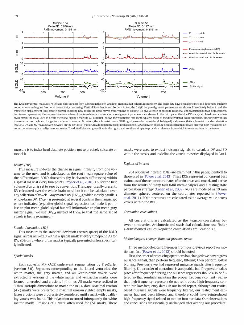
The QCmeasures employed here are largely those used in (Poweret al., 2012). Fig. 2 shows QC measures for 2 subjects. For allrealignment-estimate-derived calculations, rotational displacementswere converted to translational displacements by projection to the sur-face of a 50 mm radius sphere.

RMS motion and RMS d/dt motionThese are the root mean squared values of the detrended realign-

ment estimates and their derivatives across all timepoints.

Framewise displacement (FD)Thismeasure indexes themovement of the head fromone volume to

the next, and is calculated as the sumof the absolute values of the differ-entiated realignment estimates (by backwards differences) at everytimepoint (Power et al., 2012). FD for the first volume of a run is 0 byconvention. The purpose of this measure is to index head movement,not to precisely calculate or model it.

Absolute displacement (calculated separately for rotation and translation)These measures index the absolute displacement of the head from

the origin position at every timepoint. The translational absolute dis-placement is the sum of the absolute values of the X, Y, and Z estimatesfor a given volume. The rotational version is the sum of the absolutevalues of the displacements in pitch, yaw, and roll. The purpose of this

image of Fig.�1

BO

LDm

mm

mB

OLD

-1

1

0

2

0

50

-20

40

Volume #0 100 200 300

-1

1

0

2

0

50

-20

40

Volume #0 100 200

Framewise displacement (FD)

Absolute translational displacement

DVGS

SDGS

Global signal

Absolute rotational displacement

Subject 154Mean FD: 0.076 mm

RMS movement: 0.154 mm

Subject 53Mean FD: 0.147 mm

RMS movement: 0.319 mmX

Y

Z

pitch

yaw

roll

Fig. 2.Quality controlmeasures. At left and right are data from subjects in the low- and high-motion adult cohorts, respectively. The BOLD data have been demeaned and detrended but havenot otherwise undergone functional connectivity processing. Vertical lines denote run borders. At top, the 6 rigid body realignment parameters are shown. Immediately below in red, theframewise displacement (FD) trace is shown, indexing how much the head moves from volume to volume. To give a sense of absolute rotational and translational head displacement,two traces representing the summed absolute values of the translational and rotational realignment parameters are shown. In the third panel the blue DV trace, calculated over a wholebrain mask (the mask used to define the global signal, hence the GS subscript) shows the volumetric root mean squared value of the differentiated BOLD timeseries, indexing how muchtimeseries across the brain change from volume to volume. At bottom, the volumetric mean BOLD signal across the brain (the global signal) is shownwith its volumetric standard deviation(SD). FD, DV, and SDmeasures are elevated during periods of motion. In addition to transient displacements, SD also tracks absolute head displacement (black arrows). RMSmovement de-notes root mean square realignment estimates. The dotted blue and green lines in the right panel are there simply to provide a reference from which to see elevations in the traces.


measure is to index head absolute position, not to precisely calculate ormodel it.

DVARS (DV)This measure indexes the change in signal intensity from one vol-

ume to the next, and is calculated as the root mean square value ofthe differentiated BOLD timeseries (by backwards differences) withina spatial mask at every timepoint (Smyser et al., 2010). DV for the firstvolume of a run is set to zero by convention. This paper usually presentsDV calculated over the whole-brain mask but it can be calculated overany collection of voxels. Graymatter DV (DVGM), which closely parallelswhole-brain DV (DVGS), is presented at several points in themanuscriptwhere indicated (e.g., after global signal regression has made it point-less to plot mean global signal but still informative to plot mean graymatter signal, we use DVGM instead of DVGS so that the same set ofvoxels is being examined.)

Standard deviation (SD)This measure is the standard deviation (across space) of the BOLD

signal across all voxels within a spatial mask at every timepoint. As forDV, SD from awhole-brainmask is typically presented unless specifical-ly indicated.

Spatial masks

Each subject's MP-RAGE underwent segmentation by FreeSurfer(version 5.0). Segments corresponding to the lateral ventricles, thewhite matter, the gray matter, and all within-brain voxels wereextracted. 5 versions of the white matter and ventricular masks wereformed: uneroded, and erosions 1–4 times. All masks were resliced to3 mm isotropic dimensions to match the BOLD data. Maximal erosion(4×) masks were preferred; if maximal erosion yielded empty masks,lesser erosionswere progressively considered until amaskwith qualify-ing voxels was found. This relaxation occurred infrequently for whitematter masks. Erosions of 1 were often used for CSF masks. These

masks were used to extract nuisance signals, to calculate DV and SDwithin the masks, and to define the voxel timeseries displayed in Part I.

Regions of interest

264 regions of interest (ROIs) are examined in this paper, identical tothose used in (Power et al., 2012). These ROIs represent our current bestestimates of the center coordinates of brain areas and nuclei, and derivefrom the results of many task fMRI meta-analyses and a resting stateparcellation strategy (Cohen et al., 2008). ROIs are modeled as 10 mmdiameter spheres centered on the coordinates reported in (Poweret al., 2011). ROI timecourses are calculated as the average value acrossvoxels within the ROI.

Correlation calculations

All correlations are calculated as the Pearson correlation be-tween timeseries. Arithmetic and statistical calculations use Fisherz-transformed values. Reported correlations are Pearson's r.

Methodological changes from our previous report

Three methodological differences from our previous report on mo-tion artifact (Power et al., 2012) should be noted.

First, the order of processing operations has changed:wenow regressnuisance signals, then perform frequency filtering, then perform spatialblurring. Previously we had regressed nuisance signals after frequencyfiltering. Either order of operations is acceptable, but if regression takesplace after frequency filtering, the nuisance regressors should also be fil-tered so that residuals maintain the proper frequency content (i.e., sothat high-frequency regressors do not reintroduce high-frequency con-tent into low-frequency data). In our initial report, although our tissue-based nuisance signals were frequency filtered, our realignment esti-mates had not been filtered and therefore could have reintroducedhigh-frequency signal related to motion into our data. Our observationsand conclusions are essentially unchanged after altering our procedure.


Second, the slice-timing correction in our initial report was incorrectbecausewewere unaware that on our SiemensMAGNETOMTrio, A TimSystem 3 T scanner, interleaved acquisitions began with the secondslice (but only if the total number of slices is even). Compensation forasynchronous slice timing is now correct. As will be seen, our previousresults and conclusions are unchanged after implementing properslice timing correction.

Third, we nowuse a different andmuch larger group of subjects thanin our previous report. These subjects, though they clearly exhibit mo-tion artifact, are a selective set of subjects: they were selected out of alarger pool of subjects for the ability of their data to withstand variousvolume censoring strategies, including very stringent ones, whileretaining at least 5 min of data. Our previous dataset could not havewithstood such measures and was a higher-motion dataset.

Results

Part I: understanding BOLDmotion artifact and its relation to QC measures

The overall processing strategyAn overview of the processing strategy is shown in Fig. 1 (discussed

in Methods). This section does not involve scrubbing or iterative pro-cessing. This section describes howmotionmanifests in signal intensity,the extent to which regressions removemotion-related signal, and howQC measures reflect movement-associated signal changes.

Subject 128 S

Subject 33 S

2

0

mm

50

0

BO

LD

GM

WM

50

-50

2

0

mm

50

0

BO

LD

GM

WM

50

-50

2

0

mm

50

0

BO

LD

GM

WM

2

0

mm

50

0

BO

LD

GM

WM

0 100 200 300Volume #

0

00 100 200Volume #

10 TRs

10 TRs

GM-WM: r = 0.08GM-CSF: r = 0.16

GM-WM: r = 0.33 GM-CSF: r = -0.02

Fig. 3. QC measures and timeseries in low-motion subjects. The upper traces in each plot are aintensity plots (at left, the gray bar denotes gray matter, the white bar denotes white matter,of data, and the white text indicates the Pearson correlations between the mean gray matassociated variance is evident, though there are systematic fluctuations, of varying intensity iThese data are demeaned and detrended only, as in Fig. 2.

In this section, Figs. 2–7 contain 14 single-subject illustrations of mo-tion effects in BOLD data. We focus on single-subject data becausemotion's effects are highly variable and are therefore incompletely com-municated by peri-motion histograms or modeling. Importantly, to im-pact correlations between timeseries, motion-related signal changes donot need to be highly stereotyped, they only need to be shared acrossvoxels. Highly variable motion-related changes can alter correlationsjust as well as stereotyped motion-related changes. An understandingof the variety and magnitude of signal changes that motion can produceis quickly developed by studying individual subjects. Important aspectsof Figs. 2–7 are presented for each subject used in this report in a Supple-mental Cohort Illustration. We encourage readers to consult thisresource to develop a fuller understanding of motion-related signalchanges. The Supplemental Cohort Illustration is available at www.nil.wustl.edu/labs/petersen/Resources.html.

Quality control measuresFig. 2 shows several QC measures in 2 subjects (subjects 1–40 are

children, 41–80 are high-motion adults, 81–120 are medium-motionadults, and 121–160 are low-motion adults). Vertical lines denoteboundaries between concatenated runs. Spikes in the red FD traces in-dicate head movement, and elevations in the dotted absolute displace-ment traces indicate that the head is shifted away from the origin. Thesubject at left is generally still except for a portion of the 3rd run,where-as the subject at right moves more frequently. These subjects are

ubject 136

ubject 143

20

-20

BO

LD

20

-20

BO

LD

50

-50

50

-50

100 200Volume #

100 200Volume #

10 TRs

10 TRs

FD

DVGS

SDGS

global signal

GM-WM: r = 0.22GM-CSF: r = 0.34

GM-WM: r = 0.76GM-CSF: r = 0.55

s in Fig. 2. The timecourses of voxels in gray matter, white matter, and CSF are shown asand the yellow bar denotes CSF). In the white matter plot, the black bar indicates 10 TRster (GM), mean white matter (WM), and mean ventricular (CSF) signals. No motion-n various subjects, that presumably reflect neural activity and non-motion-related noise.

http://www.nil.wustl.edu/labs/petersen/Resources.html

http://www.nil.wustl.edu/labs/petersen/Resources.html

Subject 131 Subject 37


20

-20

BO

LD

20

-20

BO

LD

2

0

mm

50

0

BO

LD

GM

WM

50

-50

50

-50

2

0

mm

50

0

BO

LD

GM

WM

50

-50

50

-50

2

0

mm

50

0

BO

LD

GM

WM

2

0

mm

50

0

BO

LD

GM

WM

0 200 400 600Volume #

0 100 200Volume #

0 100 200Volume #

0 100 200Volume #

10 TRs10 TRs

10 TRs10 TRs

FD

DVGS

SDGS

global signal

GM-WM: r = 0.34GM-CSF: r = 0.26

GM-WM: r = 0.41GM-CSF: r = 0.53

GM-WM: r = -0.05GM-CSF: r = 0.32

GM-WM: r = 0.41 GM-CSF: r = -0.54

Fig. 4. QC measures and timeseries in subjects with intermittent movements. These subjects exhibit head movements in which the head departs from and returns to positions near theorigin (the dotted absolute displacement traces in the upper panels are not elevated). Motion-related signal changes can be brief or long. They can be decreases, increases, or complexwaveforms. They are often but not always similar across voxels. Motion-related variance is variably reflected in white matter or CSF voxels.


representative of the low- and high-motion adult cohorts (see Figure S1for mean FD distributions in each cohort).

The bottom two panels show signals and signal-derived QC mea-sures, calculatedwithin awhole brainmask in demeaned and detrendeddata, prior to nuisance regression. Other than realignment, nothing hasbeen done to counter motion-related artifact. The correspondence ofthe blue DV trace to FD is evident (DV-FD correlation across subjects(mean ± s.d.): 0.69 ± 0.38). DV does not so closely reflect absolutehead position (DV-abs. trans.: 0.32 ± 0.26; DV-abs. rot: 0.25 ± 0.23).The bottom panel shows the global signal and the SD trace. The SDtrace bears considerable similarity to the FD signal (SD-FD: 0.52 ±0.27), but also reflects absolute head position (black arrows; SD-abs.trans: 0.65 ± 0.31; SD-abs. rot: 0.54 ± 0.34). The black trace of the glob-al signal shows instances of motion-related signal changes, sometimesmanifested as decreases in signal intensity. Throughout the paper,when possible, the same QC measure color code will be used: red forFD, blue for DV, and green for SD.

Cohort properties; rationale for cohort compositionFigure S1 and Table S1 show the ages, total quantities of data, sum-

mary QC values, and statistical comparisons of the cohorts. Cohorts 1,2, and 4 (children, high-motion adults, and low-motion adults) are ofprincipal interest. Data from cohort 3, the medium-motion adults, arealso shown but will be less emphasized. The 3 principal cohorts do notdiffer in the amount of data available. The children and high-motionadults do not differ statistically on any summary QC measure, thoughthere are trends for the children to have higher RMS d/dt motion(p = 0.08) and for the high-motion adults to have higher mean SD

values (p = 0.15). These two high-motion cohorts differ from thelow- and medium-motion adult cohorts on every QC measure.

These datasets are formed for particular reasons. First, the childrenand high-motion adult cohorts are useful datasets for observing effectsof motion because motion is so prevalent. Second, if motion related ef-fects are dose-dependent, they should be similar in children and high-motion adults, modest in the medium-motion adult cohort and minorin the low-motion adult cohort. Third, if we assume that above-chancedifferences between the adult cohorts are due solely to motion, thenan effective processing strategy for removing motion-related effectsshould reduce any differences between these cohorts to chance levels.On this assumption, above-chance differences between the adult co-horts after a motion correction strategy reflect inadequate motion cor-rection and the need for further work. An alternative hypothesis isthat there exist endophenotypes detectable with resting state fMRI inpeople predisposed to move, and that a perfect motion correction strat-egy would enable detection of true and meaningful residual group dif-ferences related to this endophenotype. We cannot exclude this latterhypothesis. But we consider the former scenario much more likelyand in Parts II and III we will work toward reducing group differencesbetween the low- and high-motion adults to chance levels. To the ex-tent that this effort is successful, residual differences between childrenand adults can be interpreted as developmental and not movement-related.

The nature of motion-related varianceThe next 3 Figures summarize the effects that motion can produce

using single-subject data from12 subjects. The subjects that are presented



20

-20

BO

LD

20

-20

BO

LD2

0

mm

50

0

BO

LD

GM

WM

50

-50

50

-50

2

0

mm

50

0

BO

LD

GM

WM

50

-50

50

-50

2

0

mm

50

0

BO

LD

GM

WM

2

0

mm

50

0B

OL

DG

MW

M

0 100 200 400Volume #

0 100 200Volume #

300 0 100 300Volume #

200

0 200 300Volume #

100

10 TRs

10 TRs

10 TRs

10 TRs

FD

DVGS

SDGS

global signal

GM-WM: r = 0.71GM-CSF: r = 0.37

GM-WM: r = 0.30GM-CSF: r = 0.23

GM-WM: r = 0.38GM-CSF: r = 0.50

GM-WM: r = 0.15GM-CSF: r = 0.51

Fig. 5.QCmeasures and timeseries in subjects with shifted head position. These subjects exhibit movements that displace the head from the origin over prolonged epochs (the dotted redtraces in the top panels). SD traces reflect this absolute displacement. Timeseries reflect this displacement and are often elevated or depressed for long periods by shifted head position.


were selected for their relatively clear illustrations of particular motionsor signal changes, but they are representative of the entire dataset (seeSupplemental Cohort Illustration). All illustrated data have been de-meaned and detrended but have not undergone any further processing.

Gray matter

GM-WM GM

r: 0.33r: 0.21

0 0.5 0mean FD m

r: 0.18r: 0.05

0 2 0RMS motion RM

1

-1

Pea

rso

n r

264-

264

GS-CSF

GM-CSF

GM-WM

GS-GM

GS-WM

GS-264

Fig. 6. Pre-regression relationships between mean compartment signals, the global signal, and(GM), the white matter (WM), the ventricular (CSF), and whole-brain (GS) signals were calculof the 264 timeserieswith the global signal were calculated, aswell as themean correlation overand detrended data, as in Figs. 3–5. The values in each subject are plotted as a function of mea(black) are shown. Signal similarity, generally, is higher in subjects withmoremovement.Meanis highly correlated with the global signal.

As such, they illustrate the types of spurious variance that investigatorsseek to remove during functional connectivity processing. The top panelsdepict QC measures discussed previously. The third panels show voxeltimeseries from voxels within the gray matter mask (GM, gray bar).

Global signal Intra-gray matter

-CSF GS-WM GS-CSF GS-GM GS-264 264-264

r: 0.25r: 0.17

r: 0.32r: 0.20

r: 0.25r: 0.17

r: 0.01r: 0.01

r: 0.20r: 0.18

r: 0.19r: 0.17

0.5 0 0.5 0 0.5 0 0.5 0 0.5 0 0.5ean FD mean FD mean FD mean FD mean FD mean FD

r: 0.22r: 0.16

r: 0.17r: 0.03

r: 0.21r: 0.16

r: -0.02r: 0.00

r: 0.07r: 0.04

r: 0.07r: 0.05

2 0 2 0 2 0 2 0 2 0 2S motion RMS motion RMS motion RMS motion RMS motion RMS motion

ROI timecourses. For all 160 subjects, the indicated correlations between the gray matterated. Additionally, for 264 regions of interest, within-subject averages for the correlationsall possible pairwise correlations between the 264 ROIs. All timeseries are from demeanedn FD value and RMS motion. Linear fits including all subjects (gray) or excluding outliersFD, generally, is a better predictor of signal similarity than RMSmotion. Graymatter signal

Subject 33 Subject 37 Subject 22

DVGM

SDGM

Gray matter

Before nuisance regression

After nuisance regression

Petersen/Schlaggar:[GS GS WM WM CSF CSF ][R R ] (12 motion regressors)

Petersen/Schlaggar:[GS GS WM WM CSF CSF ][R R ](12 motion regressors)

Volterra:[GS GS WM WM CSF CSF ][R R2 Rt-1 Rt-12](24 motion regressors)

10 TRs 10 TRs 10 TRs

Volume #0 250

Volume #0 250

Volume #0 400

R = [X Y Z pitch yaw roll]

Volterra:[GS GS WM WM CSF CSF ][R R2 Rt-1 Rt-12 Rt-2 Rt-22](36 motion regressors)

FD

Fig. 7. Common regressions only partially remove motion-related variance. At top, the data from 3 subjects of Figs. 3–5 are re-presented, now with traces (DV, SD, mean signal)representing values derived from gray matter voxels only (instead of whole-brain values). Below the horizontal line, the data after 4 different regression strategies are shown. The toppanels represent the 18-parameter regression historically used in the Petersen/Schlaggar lab (12 motion-related, 6 signal-related). The next panels are the same regressors withoutthe global signal and its derivative. The next rows replace the 12 motion-related parameters with 24- and 36-parameter Volterra expansions of realignment estimates. Regardless ofthe regression strategy, the signal-derived QC measures (DV and SD) indicate artifacts in the post-regression data at periods of motion. Global signal regression visibly removes muchof the motion-related signal in addition to non-motion-related signal shared across voxels. Larger numbers of motion-related regressors capture more, but not all, motion-related vari-ance. All scales are identical to those of Figs. 3–5. Similar results are seen in Figure S3, where the same analyses are repeated with no tissue-based signals (no GS, WM, or CSF signals).


Timeseries for all voxels within the mask are presented (timeseriesare displayed in the order of the image but Matlab automaticallydownsamples the displayed data depending on plot sizing; several hun-dred voxelwise timeseries are visible). The fourth panel shows voxeltimeseries from the eroded white matter (WM, top, white bar) anderoded ventricular masks (bottom, small yellow bar).

In relatively still subjects (Fig. 3), the FD traces are flat and there is noindication from any QC measure that the data are disrupted anywherein the scan. Nevertheless, fluctuations in signal intensity are broadlyshared across voxels. These global fluctuations presumably reflectsome combination of neural activity and non-motion-related artifact,such as respiratory or cardiac effects or other influences. To the extentthat these global fluctuations are represented in white matter and ven-tricular signals, they presumably do not represent neural activity.

In subjectswhomove intermittently (Fig. 4) and return to their orig-inal position, the QC traces are mostly flat except for brief excursionsfrom the baseline. The impact of motion is variable. Some movements(white arrows) produce, acrossmost voxels, an increase then a decreasein signal, lasting many TRs (see the 10 TR scaling bar in the whitematter). Other movements (black arrows) appear not to produce anymarked effect. Still other movements (yellow arrow) produce increases

in signal. Other movements produce predominantly decreases (purplearrow). Not only the sign, but also the duration of intensity changescan vary. In the subject in the bottom left, a large movement (cyanarrow) produces a brief but marked disruption in signal, whereas inthe subject in the bottom right, several modest movements produceprolonged disruptions.

Some subjectsmove and remain displaced from the origin, as shownby sustained elevations in the absolute displacement traces in Fig. 5(dotted dark lines). These movements produce long elevations or de-pressions of signal intensity that appear as banding patterns in thevoxel intensity traces. The direction of the changes is sometimes seem-ingly uniform (black arrow), or sometimes different at different voxels(white arrows). These sustained shifts in intensity caused by shiftedhead position are qualitatively different than the intensity disruptionsresulting from head motion.

It is visually evident that signals in the gray matter, white matter,and ventricular compartments often resemble each other during mo-tion. Fig. 6 shows, for 160 subjects, the signal correlations betweenand within different tissue compartments. GM-WM and GM-CSF corre-lations are typically positive, centered about r = 0.3 and r = 0.4,respectively. Each of these compartments contributes to the global


signal, but the global signal is most strongly correlated with the graymatter signal. The similarity of signal between brain compartments,and of signals within the gray matter to other signals within the graymatter, is higher in subjects with higher FD values (except GS-GM cor-relations, which are at ceiling). Signal similarity is not as tightly relatedto RMSmotion,which reflects head position in addition to headmotion.

On the efficacy of motion-related and tissue-based nuisance regressorsMotion frequently produces fairly uniform effects across most

voxels in the brain. This observation suggests that regressors derivedfrom gray matter or all brain voxels should effectively reduce this vari-ance. Fig. 7 demonstrates this principle. Above the black line, the pre-regression data of 3 subjects from Figs. 3–5 are reproduced. Below theblack line, the gray matter voxel timeseries after several different re-gressions are displayed. Motion regression alone, even if expanded to24 or 36waveforms, does not eliminate the bulk of motion-related arti-facts. Some artifacts are visibly improved by additional regressors(black arrows) but others remain largely uncorrected (white arrows).Relatively clean signals are only obtained when the global signal andits derivative are included in nuisance regressions. However, QC tracescomputed after all nuisance regressions indicate residual artifact duringperiods of motion. This issue will be addressed in Parts II and III of thepaper.

An implication of these results is that themeanWMand CSF regres-sors are less useful than onewould hope since they were included in allregressions. Figure S3 reproduces Fig. 7 without any tissue-based re-gressors.When these Figures are compared, one is struck by themodestchanges that WM and CSF regressors produce. These results are consis-tent with previous analyses wherein WM and CSF signals explained lit-tle variance in the gray matter (Jo et al., 2010; Weissenbacher et al.,2009). The modest efficacy of WM and CSF regressors is consistentwith the moderate correlation of the WM and CSF regressors to theglobal signal (Fig. 6), which is an effective regressor.

Part I discussion: on the nature of motion-related signal changesOur observations so farmaybe summarized as follows. (1) In still sub-

jects, variance that is not apparently motion-related may be widelyshared across voxels, with variable extension to the white matter andCSF compartments. (2) Signal changes coincident with motion vary inmagnitude, andmay be widely present throughout graymatter, and var-iably, white matter and CSF voxels. (3) Complex, multi-phasic signalchanges often follow head motion. (4) Shifts in head position causesustained shifts in image intensity. (5) Phasic head motion often pro-duces pronounced effects, typically signal decreases, extending overtens of seconds after motion has ceased (dark vertical bands in Figs. 4and 5).

These signal changes are seen throughout our entire dataset (Supple-mental Cohort Illustration). The types and variety of signal changes justdescribed, including the persistent post-motion changes, are also seenin data from the Human Connectome Project (not shown), which is ac-quired using different sequences on a different scanner and processedwithout slice-time correction using different software.We therefore sus-pect that the signal changes we describe are not unique to our data.

Our findings are partially consistent with the observations ofSatterthwaite and colleagues, who reported that motion produces sig-nal decreases throughout the entire brain and that these effects scalewith the size of a movement (Satterthwaite et al., 2013). However,these authors also reported that signal depressions were largely com-plete 2 TRs (6 s) after amovement.Wefind, instead, that signal changesmaypersist for tens of seconds after amovement andare not necessarilysignal decreases. The discrepancy between our reports may arise be-cause we are visualizing highly variable signal changes across motions,time, and voxels, whereas Satterthwaite and colleagues were usingGLM analyses to identify stereotyped signal changes coincident withmotion. We note that to influence correlations, stereotyped signal

changes are not necessary, only signal changes that are shared acrossvoxels.

The variety of signal changes underscores the complexity ofmotion'seffects on BOLD signal. Shifts in head position (e.g., slow drifts, or rapidmotion without return to the original position) are associated withsustained signal changes that are variable across voxels. Motions them-selves (e.g., head nodding, speech, swallowing, etc.) are associated witha variety of transient signal changes. The signal changes at each voxelare partially but not adequately explained by position estimates fromthe current, preceding, or past 2 TRs (since regressions fail to completelyremove motion-related variance). We speculate that the variety ofchanges at a single voxel arises not only from the variety of specific mo-tions, but also from the voxel's proximity to various tissue types withdifferent signal intensities and from spin history effects. Modelingsuch interactions would be challenging.

Several implications follow from our observations. First, as we notedin our initial report (Power et al., 2012), motion-induced signal changesare generally not consistent with neural activity related to motion. Sig-nal changes are seen at almost all voxels in the gray matter and the di-rection and duration of these signal changes varies. Further, the signalchanges also occur in white matter and ventricular spaces. Some neuralactivitymust correlate withmotion and it is possible that somemotion-related activity is represented in the BOLD signal during motion, butsuch neural activity cannot account for the preponderance of signalchanges seen during and after motion. Our perspective therefore differsfrom that of (Yan et al., 2013).

Second, because prominent signal changes are highly variable andprolonged, it seems unlikely that they can be modeled by retrospectivetechniques based on relatively simple treatments of realignment esti-mates, such as regression of current or immediately preceding motionestimates. Prolonged motion-related effects must account in part forthe inability of any set ofmotion regressors thus far tested to completelyeliminate motion-related variance (Power et al., 2012; Satterthwaiteet al., 2013; Yan et al., 2013). Removal of such prolonged changes willrequiremore expansivemodeling than is typically currently performed,such as convolution of some (unknown) function with realignment es-timates, or regression of realignment estimates from many precedingtimepoints. Signal-based corrections that capture these prolonged ef-fects may prove effective in removing such variance and should receivecareful attention.

Wehave attempted several strategies to create larger andmore effec-tive sets of nuisance regressors from the white matter and ventricularvoxels, such as subdividing the masks spatially into small cubes and/orusing PCA to select several components that represent most of the vari-ancewithin themask. These efforts have not yielded encouraging results.The only procedure that produced benefits worth noting was to tempo-rally subdivide these nuisance signals (such that, for example, a 200-timepoint signal was represented as 4 50-timepoint segments). Severalversions of this temporal segmentationwere examined, all of which pro-duced modest increases in the ability of timeseries from white matterand ventricles to remove motion-related variance. However, we ulti-mately abandoned this approach because we were concerned aboutthe possible removal of signal of interest that could occur by chancewhen using such short timeseries in the regressions.

Part I focused on timeseries. The analyses in Parts II and III focus oncorrelations between timeseries. Usually the timeseries will have beenfully processed, though some analyses will examine timeseries at vari-ous steps of functional connectivity processing. In future analyses, the24-motion-parameter set of regressors will be used. This is because itis likely to be a standard for the field in the short- to medium-term fu-ture given its statistical superiority over smaller sets of motion parame-ters (Satterthwaite et al., 2013; Yan et al., 2013). We choose not to usethe 36-motion-parameter set because although it produced modestbenefits beyond the 24-motion-parameter set, it was still inadequatefor removingmotion-related effects, it requires an additional 12 degreesof freedom, and it is useful to for the coming results to be comparable

2

0

FD

Targetmasks

Positive control

Random control

2 TRsbefore FD > 0.2

1 TRbefore FD > 0.2

All motions FD > 0.2

1 TR after FD > 0.2

2 TRs after FD > 0.2



5 TRsafter FD > 0.2

0.02

0.02

r

0.02

0.02

r

Distance0 200

Distance0 200

Distance0 200

Distance0 200

Distance0 200

Distance0 200

Distance0 200

Distance0 200

N=149; 98 ± 1% N=150; 97 ± 11% N=150; 88 ± 11% N=150; 95 ± 4% N=150; 96 ± 3% N=150; 97 ± 2% N=150; 97 ± 2% N=150; 97 ± 2%

[GS GS WM WM CSF CSF R R2 Rt-1 Rt-12]

Subject 158 Subject 160A

B

No

GS

RG

SR


Random controlPositive control smoothing curveTarget mask and smoothing curve

Fig. 8. The temporal limits of motion's influence on RSFC correlations. This analysis reveals the impact on RSFC correlations of volumes acquired before, during, and after headmotion. A) Illus-trations of temporal masks in two subjects. B) For completely processed data prepared without GSR (top) and with GSR (bottom), the effects of each mask in (A) are shown. Δr is calculatedacross all subject impacted by a particular mask. The number of subjects impacted by a mask and the mean and standard deviation of remaining data are shown for each analysis (e.g., theN =150 for the 3rdmaskmeans that 150/160 subjects had some volumes with FD N 0.2 mm, and the 10/160who did not were not included inΔr calculations). TRs prior to motionwere ex-amined because frequencyfiltering can spread artifact backward and forward in time, and TRs subsequent tomotionwere examined especially due to the prolonged signal changes seen in Fig. 4.


with other recent reports that utilize the 24-motion-parameter set ofregressors (Satterthwaite et al., 2013; Yan et al., 2013). Additionally,most future analyses will include data processed with and withoutGSR given the visible efficacy of this regressor (Fig. 7) and the recent re-ports on its utility for removing motion artifact (Satterthwaite et al.,2013; Yan et al., 2013). Since the field continues to debate the use ofGSR (Fox et al., 2009; Murphy et al., 2009; Saad et al., 2012), analyseswith and without GSR will provide investigators of all viewpoints withempirical evidence on the efficacy of their preferred approach to artifactremoval.

Part II: understanding how motion impacts RSFC correlations

It is established that motion produces systematic changes in RSFCcorrelations (Power et al., 2012; Satterthwaite et al., 2012; Van Dijket al., 2012). This section seeks to answer several outstanding questionsrelated to motion and RSFC correlation structure: (1) whether theprolonged signal disruptions after motion systematically impact RSFCcorrelations; (2) whether absolute head displacement systematicallyimpacts RSFC correlations; (3) whether stricter censoring thresholdsproduce greater removal of artifactual RSFC structure; (4) whetherhigh values on all QC measures identify similar artifactual properties;(5) whether ‘improvements’ in a volume over processing are completeor partially cosmetic (i.e., does a volume with high DV values beforeprocessing but normal DV values after processing now contributeRSFC structure that resembles ‘random’ data or does it still resemblehigh-DV data); and (6) whether a threshold or inflection point can befound in a QC measure, below which artifactual influences are negligi-ble. The answers to these questions will guide the formation ofsubject-level censoring-based strategies of artifact correction in Part III.

In our initial report on motion (Power et al., 2012), to characterizethe impact of motion on correlations, we compared correlations in full

timeseries to correlations in timeseries from which high-motion vol-umes had been deleted. This censoring procedure was called ‘scrub-bing’, a term that refers to the practice of discarding incorrect oruntrustworthy pieces of information. In our initial report censoringwas only done during correlation calculations, but it can be incorporat-ed into data processing steps such as regressions and temporal filtering(Carp, 2013; Power et al., 2011, 2012, 2013; Satterthwaite et al., 2013).Certain characterizations of high-motion data (as in Fig. 11B) cannot beperformed if the data have been censored or replaced. Therefore, in thissection we censor only after functional connectivity processing is com-plete. Iterative processing with censoring incorporated throughout theprocessing stream is described in Part III.

Several analyses in this section use scrubbing to characterize the im-pact of particular parts of data on RSFC correlations. These analyses ex-amine the changes in correlation produced in all possible pairwisecorrelations (34,716) between the 264 ROIs reported in (Power et al.,2011)when particular portions of the data arewithheld from correlationcalculations. Across-subject changes in correlation are reported (Δr =mean scrubbed r − mean unscrubbed r). Within-subject analyses(Δr = mean (scrubbed r − unscrubbed r)) produced nearly identicalresults and are not shown. Within-subject analyses that were normal-ized to the amount of data removed per subject produced similar resultsand are not shown. In subsequent Figures, Δr will be plotted for eachpairwise correlation as a function of the Euclidean distance separatingthe center coordinates of the ROIs that gave rise to the correlation.

The temporal extent of motion's impact on RSFC correlationsThe prolonged signal changes seen in Fig. 4 suggest thatmotionmay

influence RSFC correlations for many TRs after the head has ceasedmoving. To investigate this issue, 8 ‘target’ temporal masks wereformed in each subject. Each target mask identified a particular typeof individual volume, such as volumes prior to, during, or after motion.


Such masks are illustrated for 2 subjects in Fig. 8A. The ‘target masks’bar contains 8 rows, each representing a temporalmask. Rows 1–2 indi-vidually identify the 2 TRs prior to motion, row 3 identifies motion(FD N 0.2 mm), and rows 4–8 individually identify the 5 TRs after mo-tion. A set of ‘positive control’ masks was also created, one for each ofthe target masks. Each ‘positive control’ mask removes, within eachsubject, identical amounts of data by FD rank (e.g., if a ‘target mask’ re-moved 8 volumes, the corresponding ‘positive control’ mask removedthe 8 volumes with the highest FD values in the scan). A set of ‘randomcontrol’ masks removes, for each ‘target mask’ within each subject,identical amounts of data but at randompoints in the scan. The ‘positivecontrol’ showswhat changes in correlation are possiblewhen removinga given amount of data (because sometimes very little data is removed),and the ‘random control’ shows that correlation changes are specific tothe type of volume identified by a target mask.

The temporal extent of the influence of motion on RSFC correlationsis shown in Fig. 8B. Here, for each of the 8 types ofmask described above,the Δr for each pairwise relationship is plotted by the distance betweenthat pair of ROIs.Without GSR,motion's influence is evident in the 4 or 5

Motion

Rando

OriginalFD < 0.5

FD < 0.2

15

0Sig

nific

ant h

igh-

vs.

low

-m

otio

n ad

ult d

iffer

ence

sp

< 0

.000

05

N: 4096 ± 6

0.1

-0.1

r

0.1

-0.1

r

0.1

-0.1

r

0 200Distance

0 20Distance

N: 4082 ± 12

N: 4097 ± 2

N: 4081 ± 8

N: 40 98 ± 2


FD > 0.5 mm FD > 0.2 mm

Cohort 4: Low-motion

adults

Cohort 2: High-motion

adults

Cohort 1:Children

N: 40 100 ± 0

Fig. 9.Motion scrubbing selectively decreases group differences. These plots show, for analyseproducedby FD-targeted scrubbing in various cohorts at various thresholds (a lenient thresholdin the analysis, and the numbers below indicate the mean and standard deviation of the percebetween low-motion and high-motion adult cohorts is shown, out of ~35,000 pairwise correlatidard deviations across 30 repetitions of random censoring. Comparisons of all adult cohorts at oyses, unlike other Figures,meanΔr is calculated across all subjects in a cohort, regardless ofwhetwould actually be seen in cohorts upon scrubbing an entire dataset.

TRs (10–12.5 s) following a motion. With GSR, motion's influence is es-sentially restricted to the period of movement. These effects were calcu-lated in all subjects with data removed by a given mask (N = 150);within-subject analyses yielded virtually identical results (data notshown). An informative feature of these analyses is that no artifact isseen in the TRs prior tomotion, indicating that our gentle (and symmet-ric) frequency filtering did not result in noticeable temporal spread ofartifact into adjacent TRs. Figure S4 extends these analyses to the 10TRs following motion and to timeseries from various steps in functionalconnectivity processing (pre-regression, post-regression, and finaltimeseries). Similar effects are seen at all stages of processing. Theseanalyses indicate that, in our data, motion impacts correlations mainlyin the 4 TRs (10 s) after a movement. The analyses in Figure S4 also in-clude amask that identifies volumes temporally distant frommotion (atleast 10 TRs after FD N 0.2 mm) that have absolute displacements over0.5 mm. Censoring with this mask reveals no obvious structured influ-ence of absolute head displacement on RSFC correlations, indicatingthat the sustained signal changes produced by absolute head displace-ment seen in Fig. 5 are largely corrected by existing regression strategies.

-targeted censoring

m censoring

0

OriginalFD < 0.5

FD < 0.2

1500

Sig

nific

ant h

igh-

vs.

low

-m

otio

n ad

ult d

iffer

ence

s p

< 0

.000

05

0

0.1

-0.1

r

0.1

-0.1

r

0.1

-0.1

r

0 200Distance

0 200Distance

N: 4096 ± 6

N: 4082 ± 12

N: 4097 ± 2

N: 4081 ± 8

N: 40100 ± 0

N: 4098 ± 2


FD > 0.5 mm FD > 0.2 mm

s with GSR (left) and without GSR (right), the distance-dependent changes in correlationof FD N 0.5 mmand a strict threshold of FD N 0.2 mm). N indicates the number of subjectsntage of data remaining after scrubbing. At bottom, the number of significant differencesons, as determined by a two-sample t-test. The error bars on the random bars are the stan-ther statistical thresholds yield similar patterns and are shown in Figure S5. In these anal-her any volumeswere censored, to illustrate the types of ‘bottom line’ changes in RSFC that


However, only 20 subjects exhibited isolated absolute head displace-ment, and we therefore consider this conclusion to be provisional.

The effect of censoring stringency in different populationsAn important question is the extent to which different populations

exhibit motion-related biases in RSFC. Relatedly, we have posited thatabove-chance group differences between high-motion and low-motionadults are at least partially, and perhaps entirely, due to motion. Weare therefore interested in the extent to which different populations dis-play motion-related effects, and the extent to which various processingstrategies reduce group differences.

The effects of lenient (FD N 0.5 mm) and stringent (FD N 0.2 mm)FD-based scrubbing are shown in Fig. 9. With GSR, children display ef-fects at both thresholds, high-motion adults display effects only at thestringent threshold, and low-motion adults display effects at neitherthreshold. Importantly, FD-based scrubbing reduces group differencesbetween the high- and low-motion adults. This effect is specific tohigh-FD volumes: random volume removal produced no such effect.This effect is seen regardless of statistical threshold used to definegroup differences, and the selective reduction in group differences isseen in all comparisons of all adult cohorts (Figure S5).

Without GSR, similar effects are seen aswith GSR, except that effectscan now be appreciated in the high-motion adults at lenient thresholds,and in the low-motion adults at stringent thresholds (the red fringesbelow the black points in both plots). Here, too, FD-targeted scrubbingselectively reduces groupdifferences. Note also the scale of group differ-ences: for a given statistical threshold, using identical temporal masks,the number of significant differences without GSR is nearly 2 orders ofmagnitude greater. These findings hold regardless of statistical thresh-old or the adult groups compared (Figure S5). The elimination ofgroup differences by various processing strategies will be revisited inPart III.

Pre-regression

Post-regression

Temporally filtered

Spatially blurred

Subject 73

DVGM

DVGM

DVGM

DVGM

26

19

6

3

0

2

0

50

0

50

0

20

0

10

0

2

0

50

0

50

0

20

0

10

BO

LDB

OLD

BO

LDB

OLD

mm

0 200 400 0

Volume #

0.5

Fig. 10.An illustration of the evolution of signal-basedQCmeasures through functional connectiare shown at different steps of functional connectivity processing. DV and SD traces evolve ththreshold 2 standard deviations above the median value (the number beside the plot). At righthresholds displayed at left. QC values from any stage of processing produce temporalmaskswiteffects are seen when timeseries from any stage of processing are censored (data not shown).

On using DV and SD to censor dataFD, DV, and SD are all possible QCmeasures. Thus far, we have charac-

terized data using FD. We now turn to the other QCmeasures, which dif-fer from FD in important ways. FD is based on realignment estimates andtherefore is unaffected by subsequent processing steps. DV andSD, in con-trast, derive from BOLD intensity, and may evolve through processing(Fig. 10). Before processing, DV strongly resembles FD, but this similaritydiminishes with processing (DV–FD pre-regression: r = 0.69 ± 0.34;post-regression: r = 0.23 ± 0.28; post-frequency filtering: r = 0.17 ±0.27; post-spatial blurring: r = 0.18 ± 0.25). Some peaks in the DVtrace are abolished, others are reduced, others remain. The same is truefor SD values (SD–FD pre-regression: r = 0.52 ± 0.27; post-regression:r = 0.07 ± 0.29; post-frequency filtering: r = 0.07 ± 0.27; post-spatial blurring: r = 0.04 ± 0.24). Before regression SD traces uniquelydisplay plateaus and scalloping corresponding to absolute head position,but after regression the scalloping and plateaus are largely eliminated,possibly reflecting the efficacy of existing regressions in correcting arti-facts attributable to absolute displacement. It may be advantageous touse QC measures that track evolving data quality rather than an un-changeable trace of head motion. For example, a temporal mask madeusing DV after functional connectivity processingmight appropriately re-tain more (denoised) data than a mask formed using FD (which cannotreflect denoising).

These considerations prompt two questions. First, do volumes withoutlying DV and SD values produce changes in correlation similar towhat has been seen in FD-based analyses? The right side of Fig. 10 an-swers the first question. Outlying values of either DV or SD, at anystage of processing, when used to censor fully processed timeseries,produce the familiar distance-dependent effects seen with FD-basedanalyses. This is true regardless of the step in processing at which corre-lations are calculated (e.g., in pre-regression or pre-frequency-filteringtimeseries; data not shown). Thus, the elevations in QC traces identifydata with similar characteristics at all times.

Subject 73

SDGM

SDGM

SDGM

SDGM

Euclidean Distance

0 200 0 200-0.1

0.1

r

-0.1

0.1

r

-0.1

0.1

r

-0.1

0.1

r

-0.1

0.1r

Cohort 1

24

15

9

4.6

200 400

Volume #

0.2

vity processing. At left, for a single subject, FD traces are shown at top, andDVand SD tracesroughout processing. For DV and SD, the horizontal lines represent, across all subjects, at, in Cohort 1, the across-subject Δr (N = 40) produced by censoring volumes above theh similar effects. These results are obtained by censoring fully processed timeseries; similar


Second, the reduction or elimination of some peaks in QC tracesprompts the question of whether volumes that ‘improve’ in QC valuesover processing are truly corrected or whether such changes are cos-metic. In other words, if a volume begins with an outlying DV valueand then acquires a more typical DV value later in processing, doesthat volume's impact on RSFC correlations now resemble that of a typi-cal volume (from a period of stillness), or does it continue to resemblethe impact of an outlying volume (from an ‘uncorrected’ period ofmotion)?

Full descriptions of the analyses that answer this question are pro-vided in the Supplemental Materials and Figure S6, but the unfortunateanswer is that DV improvements are partially cosmetic, and data thatbegin with an elevated value that decreases throughout processingmany still harbormotion artifact (Fig. 11A). Initial QC values before pro-cessing are therefore themost reliable indicator of data quality. BecauseSD reflects absolute head position, which does not clearly impact RSFCcorrelations (Figure S4), and because its motion-tracking characteristicsare otherwise largely represented by FD and DV (Fig. 10), we do notpursue further analyses using SD. Thus, the remainder of this paper fo-cuses on using FD and initial DV values to make processing decisions.

On relating QC values to significant changes in RSFC correlationsUntil more efficacious artifact removal techniques are demonstrated,

nuisance regression alonewill be inadequate for subject-level correctionof motion's effects. A further step that can be taken at the subject level isto entirely discard motion-corrupted volumes. This approach sacrificesdata but it is also effective in eliminating motion-related variance(Power et al., 2012, 2013; Satterthwaite et al., 2013). An important ques-tion is: what data should be censored? We reframe the question as: atwhat QC values do significant within-subject changes in correlation be-come evident?

Full descriptions of the approach and analyses developed to answerthis question are presented in Supplemental Materials and Figure S7.The top panel of Fig. 11B shows the gist of the analyses, wherein asubject's data are ordered by decreasing quality and the changes in cor-relation observed going from the best to the worst data are plotted.Whether such changes are significant is empirically determined by re-peating this procedure with random orderings of the data (irrespectiveof QC values). The green points are insignificant changes in the QC-ordered data, the red points are significant changes, and theblack pointsare from the random permutations that define empirical significance.

-0.002

0.002

r

0 200Distance

Random scrubbing (negative control)

DV scrubbing (positive control)

values that had very high pre-regression DV values

0

Highe

0

100

Ran

k (%

)

-0.1

0.1

r

A B

Fig. 11. A) Scrubbing of volumes that begin with high outlying DV values before functional connfollowing nuisance regression. The timeseries are post-regression, pre-frequency-filtering (othwithin-subject changes in mean short-distance correlation seen in a 50-volume sliding windopoints establish random expectations, and are produced by random orderings of the data. BottQC ranges. Rank bins are 0–100% in 5% bins. With 20 rank bins, 5% of the data should fall in eachacross subjects.

When this procedure is repeated for all 160 subjects the resulting em-pirical ranks can be plotted as a function of QC value, as in the bottompanel of Fig. 11B. This plot indicates that significant within-subjectchanges in correlation are detectable down to FD = 0.15–0.2 mm andare very pronounced at FD = 0.5 mm.

The analyses shown in Figs. 11B and S7 indicate that high, outly-ing values on QC measures (e.g., FD = 0.5 mm, or pre-regressionDV = 20) unquestionably are associated with within-subject eleva-tions in short-distance correlations. Most data have QC values notassociated with such artifactual elevations in correlation (see the cu-mulative distribution curves, the black sigmoid trace in Fig. 11B). Onthe basis of these results, one could argue that very strict thresholds,excluding QC values beyond even a hint of a skew (FD N 0.15 or pre-regression DV N 13) are ideal. Most datasets will not tolerate censor-ing based on such strict thresholds, nor it is obvious that this par-ticular analysis should be the only criterion for setting thresholds.We interpret these results to support the general principle that thestricter one sets thresholds for censoring, the more one can guardagainst or eliminate motion-related artifact.

Part II discussion: on motion's influence on RSFC correlationsThe key observations of this section are: (1) effects ofmotionmanifest

in RSFC correlations for ~10 s after motion; (2) post-motion effects areessentially eliminatedwhenGSR is performed; (3) absolute displacementdoes not appear to produce systematic changes in RSFC correlations;(4) stricter censoring thresholds remove larger amounts of distance-dependent artifact; (5) distance-dependent artifact is present with orwithout GSR; (6) motion scrubbing selectively reduces motion-relatedgroup differences in adult cohorts; (7) improved QC values do not guar-antee that the data are fully corrected; and (8) QC values can be quantita-tively linked to the significance of changes inRSFC correlations, butwe areunable to point to a single value of FDor initial DVas adefinitive thresholdbeyond which data are compromised— the effect is gradual.

Part III: processing data in ways that minimize motion-related influences

In this section,we use thefindings of Part II tomodify our processingstream to more powerfully suppress motion artifact at the subject level.We assess the ability of this processing stream to eliminate detectableinfluences of motion and group differences that are attributable tomotion.

10.2 0.4 0.6 0.8

st FD value within sliding window

% of data at a given QC bin (horizontal)in a given rank bin (vertical)

50

0

ectivity processing but which then exhibit DV values within 1 s.d. of themedian DV valueer stages showing similar effects are shown in Figure S6). B) Top, for a single subject, thew are shown as a function of the highest FD value found within each window. The blackom, a heat map showing the across-subject distribution of empirical ranks within binnedrank bin by chance. The black sigmoidal trace is the cumulative distribution of datapoints


Incorporating censoring into an iterative processing strategyWe now adopt a strategy where the data are processed as in Parts I

and II, then QC measures are derived and used to form temporalmasks, and then the data are re-processed using the temporal masksto censor data (Fig. 1, dotted gray lines). The principal features of the it-erative processing strategy are: (1) censoring is incorporated into de-meaning and detrending each run, (2) censoring is incorporated intothe multiple regressions performed across runs, (3) temporal masksare used to define data that are replaced by interpolation, prior to fre-quency filtering, and (4) the interpolated data are recensored followingfrequency filtering.

In this iterative scheme, 4 steps are used to form the temporalmasksused to reprocess the data (see Figure S8 for an illustration in a singlesubject). Step 1: volumes with FD N 0.2 mm or initial DV N 20 werecensored. Step 2: uncensored segments of data lasting fewer than 5 con-tiguous volumes as a result of Step 1 were censored. Step 3: runs withfewer than 50 remaining volumes were entirely eliminated. Step 4:subjects with less than 125 uncensored volumes across runs were elim-inated. This procedure eliminated entire runs in 5 children and 2 high-motion adults; 3 children were removed for insufficient remainingvolumes across runs. Overall, 83% ± 17% (range 28%–100%) of thedata were retained (Figure S8). To investigate the impact of interpola-tion, the data were reprocessed both with and without this step. Fullyprocessed timeseries were often similar with and without interpolation(Figure S9). However, in several instances where motion occurred,reprocessing without interpolation yielded anomalous timeseries fea-tures (Figure S9). These anomalies occurred because outlying values inthe censored timepoints were neither ameliorated by regression (be-cause they did not contribute to regressor fits) nor were they replacedby interpolation, and they could therefore spread large-amplitude arti-factual signals into adjacent TRs during frequency filtering. We there-fore only focus on data that are reprocessed including interpolation;hereafter ‘reprocessed’ refers to data reprocessed with interpolation.

Other criteria could have been used to form temporal masks andsome differences with our previous report should bementioned. In par-ticular, here we did not augment temporal masks (expanding them for-ward and backward in time) because we are principally interested inresults usingGSR, which exhibited no impacts ofmotion on correlationsin TRs before or after motion (Fig. 8). Analyses done without GSR maybenefit from censoring several TRs after head movement (such aug-mented masks are examined where appropriate below). The require-ments for some number of contiguous volumes (Step 2) and aminimum number of within-run volumes (Step 3) have no particular

QC

-RS

FC

r

-0.5

0.5

# co

rrel

atio

ns

4000

0-0.5 0.5QC-RSFC r -0.5 0.5QC-RSFC r -0.5 0.5QC-RSFC r

Distance Distance Distance0 200 0 200 0 200

Unscrubbed Scrubbed Reprocessed


QC-RSFC correlation

QC-RSFC correlation

Fig. 12. Scrubbing and reprocessing reduce QC-RSFC correlations. For all 120 adults, mean FD wgimes. The histograms plot the observed and random QC-RSFC relationships observed under e

empirical support. The need for 125 volumes across runs (Step 4) arisesfrom the conventionalminimumof ~5 min of data for computing corre-lations (Van Dijk et al., 2010).

Evaluating reprocessed data for evidence of motion artifactOne way of assessing RSFC data for evidence of motion artifact is to

correlate a vector of summary QC values (e.g., mean FD or RMSmotion)with vectors of outcome measures across subjects. This linear depen-dence is what is removed by group-level corrections implemented bylinearly regressing summary QC measures out of outcome measuresacross subjects (Satterthwaite et al., 2012, 2013; Van Dijk et al., 2012;Yan et al., 2013).We refer to these correlations as QC-RSFC correlations.

QC-RSFC correlations across 120 adults are shown for several pro-cessing strategies in Fig. 12, using mean FD as a summary QC measure.In unscrubbed data prepared with GSR, short-distance correlations arepositively correlated withmean FD.With scrubbing, these relationshipsare reduced, and with reprocessing, they are almost absent. WithoutGSR, correlations at all distances are positively related to mean FD andthese relationships can be reduced but not eliminated by scrubbingand reprocessing. Reprocessing datawith temporalmasks that also cen-sored the 4 volumes subsequent to FD N 0.2 mm did not alter results(data not shown).

Between-cohort differences can be reduced to chance levels by scrubbingAnother way to assess the efficacy of within-subject motion correc-

tion is to examine group differences under various processing strategies.We have created 3 adult cohorts that differ bymean FD. Comparisons ofall groups yield significant group differences (Figure S5). We now ex-amine the extent to which different processing strategies reduce thesegroup differences, which are in part, if not entirely, due to motion.

The observed numbers of adult groupdifferences under different pro-cessing strategies are presented in Figs. 13 and S10. Null expectationswere established by 10,000 permutations of adult subject identity. Ingeneral, scrubbing eliminated many group differences, and reprocessingfurther reduced group differences.Without GSR, these steps reduced butdid not eliminate group differences. With GSR, reprocessing reducedgroup differences to chance levels at most statistical thresholds (in 8 of9 analyses, Figure S10).

These results indicate that within-subject corrections may be capa-ble of adequately correcting for motion without a need for group levelcorrection. It is possible that other versions of censoring wouldoutperform the current approach. Indeed, since this is the first attemptwe have made at a comprehensive approach to censoring, it would be


-0.5 0.5QC-RSFC r -0.5 0.5QC-RSFC r -0.5 0.5QC-RSFC r

Distance Distance Distance0 200 0 200 0 200


using mean FD

using randomly permuted mean FD

as correlated across subjects with each pairwise correlation under several processing re-ach processing stream.

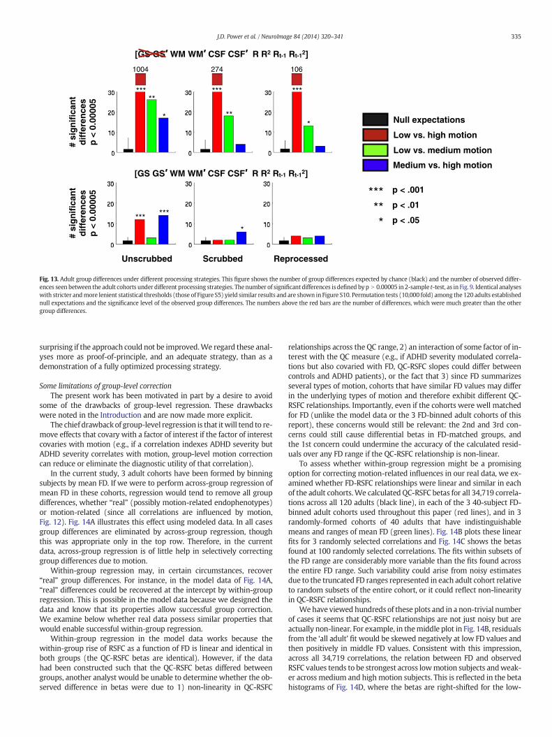
Low vs. high motion

Low vs. medium motion

Medium vs. high motion

Null expectations

*** p < .001

** p < .01

* p < .05

*****

*

***

**

***

*

1004 274 106

*** ***

*




# si

gn

ific

ant

dif

fere

nce

sp

< 0

.000

05

# si

gn

ific

ant

dif

fere

nce

sp

< 0

.000

05

Fig. 13. Adult group differences under different processing strategies. This figure shows the number of group differences expected by chance (black) and the number of observed differ-ences seen between the adult cohorts under different processing strategies. Thenumber of significant differences is defined byp N 0.00005 in2-sample t-test, as in Fig. 9. Identical analyseswith stricter andmore lenient statistical thresholds (those of Figure S5) yield similar results and are shown in Figure S10. Permutation tests (10,000 fold) among the 120 adults establishednull expectations and the significance level of the observed group differences. The numbers above the red bars are the number of differences, which were much greater than the othergroup differences.


surprising if the approach could not be improved.We regard these anal-yses more as proof-of-principle, and an adequate strategy, than as ademonstration of a fully optimized processing strategy.

Some limitations of group-level correctionThe present work has been motivated in part by a desire to avoid

some of the drawbacks of group-level regression. These drawbackswere noted in the Introduction and are now made more explicit.

The chief drawbackof group-level regression is that itwill tend to re-move effects that covary with a factor of interest if the factor of interestcovaries with motion (e.g., if a correlation indexes ADHD severity butADHD severity correlates with motion, group-level motion correctioncan reduce or eliminate the diagnostic utility of that correlation).

In the current study, 3 adult cohorts have been formed by binningsubjects by mean FD. If we were to perform across-group regression ofmean FD in these cohorts, regression would tend to remove all groupdifferences, whether “real” (possibly motion-related endophenotypes)or motion-related (since all correlations are influenced by motion,Fig. 12). Fig. 14A illustrates this effect using modeled data. In all casesgroup differences are eliminated by across-group regression, thoughthis was appropriate only in the top row. Therefore, in the currentdata, across-group regression is of little help in selectively correctinggroup differences due to motion.

Within-group regression may, in certain circumstances, recover“real” group differences. For instance, in the model data of Fig. 14A,“real” differences could be recovered at the intercept by within-groupregression. This is possible in the model data because we designed thedata and know that its properties allow successful group correction.We examine below whether real data possess similar properties thatwould enable successful within-group regression.

Within-group regression in the model data works because thewithin-group rise of RSFC as a function of FD is linear and identical inboth groups (the QC-RSFC betas are identical). However, if the datahad been constructed such that the QC-RSFC betas differed betweengroups, another analyst would be unable to determine whether the ob-served difference in betas were due to 1) non-linearity in QC-RSFC

relationships across the QC range, 2) an interaction of some factor of in-terest with the QC measure (e.g., if ADHD severity modulated correla-tions but also covaried with FD, QC-RSFC slopes could differ betweencontrols and ADHD patients), or the fact that 3) since FD summarizesseveral types of motion, cohorts that have similar FD values may differin the underlying types of motion and therefore exhibit different QC-RSFC relationships. Importantly, even if the cohorts were well matchedfor FD (unlike the model data or the 3 FD-binned adult cohorts of thisreport), these concerns would still be relevant: the 2nd and 3rd con-cerns could still cause differential betas in FD-matched groups, andthe 1st concern could undermine the accuracy of the calculated resid-uals over any FD range if the QC-RSFC relationship is non-linear.

To assess whether within-group regression might be a promisingoption for correcting motion-related influences in our real data, we ex-amined whether FD-RSFC relationships were linear and similar in eachof the adult cohorts.We calculated QC-RSFC betas for all 34,719 correla-tions across all 120 adults (black line), in each of the 3 40-subject FD-binned adult cohorts used throughout this paper (red lines), and in 3randomly-formed cohorts of 40 adults that have indistinguishablemeans and ranges of mean FD (green lines). Fig. 14B plots these linearfits for 3 randomly selected correlations and Fig. 14C shows the betasfound at 100 randomly selected correlations. The fits within subsets ofthe FD range are considerably more variable than the fits found acrossthe entire FD range. Such variability could arise from noisy estimatesdue to the truncated FD ranges represented in each adult cohort relativeto random subsets of the entire cohort, or it could reflect non-linearityin QC-RSFC relationships.

We have viewed hundreds of these plots and in a non-trivial numberof cases it seems that QC-RSFC relationships are not just noisy but areactually non-linear. For example, in themiddle plot in Fig. 14B, residualsfrom the ‘all adult’ fit would be skewed negatively at low FD values andthen positively in middle FD values. Consistent with this impression,across all 34,719 correlations, the relation between FD and observedRSFC values tends to be strongest across lowmotion subjects andweak-er across medium and high motion subjects. This is reflected in the betahistograms of Fig. 14D, where the betas are right-shifted for the low-

rr

r

A B

C

D

FD FD FD

Low-motion cohort

High-motion cohort

3 random cohorts (FD-matched, N = 40)

3 adult cohorts (FD-binned, N = 40)

beta

All adults

Random (3 cohorts)Adults (3 cohorts)

-1

1.5

FD FD FD

r

-0.5

1

Pairwise correlation # (randomly selected, sorted by all-subject beta)1 100

All adults (N = 120)

Correlation values

0 0.25 0 0.25 0 0.25

Beta

All adults

Random High-motion

1-1

Medium-motion

Low-motion

values values

Across-group ‘Observed’‘True’

corrected

Within-group

corrected

FD

Across-group linear fit

Within-group linear fit

r

Fig. 14. Some limitations of group-level regression. A) A diagram of how across-group and within-group regression may andmay not correct artifactual increases in correlations. In thesesimulations, a ‘true’ value is specified for each cohort, as is an FD distribution (low-motion and high-motion). ‘Observed values’ are computed by adding a constant beta multiplied by thesubject's FD value to the ‘true’ value. ‘Across-group corrected’ values reflect residuals after a linear fit is made across both cohorts, and ‘within-group corrected’ values reflect residuals(intercepts retained) after a linear fit is made within each cohort. The ‘within-group’ correction works because the rise in r per unit FD is linear and identical in both groups. B) For 3 ran-domly selected pairwise relationships, the RSFC correlations (without GSR) of 120 adult subjects are plotted as a function of each subject's mean FD. Lines show linear QC-RSFC fits ondifferent subsets of the data, including all subjects (black), the actual FD-binned cohorts of the paper (red), and randomly-formed 40-subject cohorts that have indistinguishable meanFD distributions. C) The beta values at 100 randomly selected pairwise correlations are shown. D) Across all pairwise correlations, the distribution of beta values in the different cohortsof (B, C). The betas in the low-motion cohort are higher and span a broader range of values than the betas found in the other cohorts. These datawere prepared using regressors [WMWM′

CSF CSF′ R R2 Rt − 1 Rt − 12 ].


motion cohort relative to the other cohorts. This result suggests that inmany correlations we cannot assume a linear QC-RSFC relation acrossthe range of our QCmeasure. This finding calls into question the accura-cy of the residuals obtained after regression across all subjects (the blackor green lines), and it also indicates that in real data, within-group re-gression will obtain differential QC-RSFC betas in the adult cohorts(red lines) and is therefore unlikely to produce the desired types of cor-rections illustrated in Fig. 14A.

Discussion

Important points from Parts I and II were discussed at the close ofeach section. This Discussion therefore focuses on the results of Part IIIand the implications of the report as a whole.

On the use of group-level correction

If GSR (or some equivalently effective subject-level correction) is notperformed, some other technique is needed to control for motion-related group differences. Group-level regression has been proposedas a corrective measure (Satterthwaite et al., 2012; Van Dijk et al.,2012; Yan et al., 2013). It is important to note that QC-RSFC betas differat different portions of the mean FD range. In the current data, this

nonlinearity would cause mean FD, for a given pairwise correlation, toact differently as a regressor in the different adult cohorts, since the co-horts occupied different portions of themean FD range. If within-groupregression is performed, it is therefore advisable to match cohorts notonly on mean QC values, but also on ranges of summary QC values inorder to (presumably) obtain homogeneity of regression slopes. Evenso, depending on the range of motion, although a linear fit may beobtained, the underlying data may not actually be linearly dependenton motion, and it is also possible that differential betas will still befound even in well-matched groups (concerns 2 and 3 above).

On the implementation of censoring

Several groups have found a benefit of censoring high-motion data(Power et al., 2012; Satterthwaite et al., 2013; Yan et al., 2013). Thisbenefit accrues because all nuisance regressions thus far examinedhave failed to adequately model or remove motion-related variance.Until improved motion correction strategies are devised, censoringwill be a useful tool for reducing or eliminatingmotion-related variancein resting state timeseries.

It is important to recognize that someminimumamount of datamustremain after censoring. The field accepts ~5 min of data as an adequatestarting point for RSFC analyses (Van Dijk et al., 2010). Accordingly, we


required that 125 volumes (5.2 min) remain after censoring for inclusionin our analyses. Because we started with several hundred volumes ofdata in most subjects, this requirement was easily met, and we typicallyhad several hundred volumes of data remaining in our subjects evenafter strict censoring strategies.

As noted in the Introduction, thedatasets included in this studywerechosen for their ability to withstand such strict censoring strategies. Inthis paper, few subjects were eliminated in any analysis because ofthis selection bias. In other completed and ongoing studies we do elim-inate subjects: in studies of normal adults, we eliminate perhaps 10% ofour subjects; in pediatric and clinical studies, the proportion can exceed30%. This loss of subjects is regrettable but difficult to avoid if within-subject correction is to be used. We have, over the last two years,begun to collect more resting state data from each subject, in longerruns, so that more subjects qualify for correction by censoring.

We do not advocate relaxing the quantity requirement much below125 volumes (~5 min) in order to salvage subjects. Removing timepointsincreases the sampling error of estimated correlations. In the scrubbinganalyses, the addition of white noise by censoring is illustrated by therandom Δr analyses that yielded a Gaussian distribution of black pointscentered on zero.

A related issue is how to deal with degrees of freedomwhen censor-ing, since the number of timepoints contributing to outcome measurestypically differs across subjects after censoring. One way to address thisproblem is to reduce all temporal masks to the same length (e.g., theminimum length found across subjects in a study). We have found thatsuch ‘trimming’ of temporal masks can have an impact when techniquessuch as multivariate pattern analysis are used to classify individuals thatdiffer in the amount of data available (unpublished observations). Inother group-level applications, such as mean seed maps or meanpairwise correlations, especially when calculated over many subjectsand in datasets with many hundreds of post-scrubbing volumes inmost subjects, such ‘trimming’ appears to make little difference. For ex-ample, reanalysis using trimming (to 126 volumes) made no differencein the group difference results of Fig. 13 (data not shown). The additionalremoval of volumes must be balanced against the degrees of freedomavailable in a dataset and the degrees of freedom required by a process-ing stream (which is influenced by autocorrelation, nuisance regression,the presence and type of frequency filtering, etc.).

Another issue worth mentioning is the interaction of temporal dy-namics with censoring. The detection and characterization of dynamicstates in resting state MRI are an increasingly examined topic (Changand Glover, 2010; Smith et al., 2012), and some objections to censoringhave been raised on the grounds that censoring might decrease contri-butions to correlations from certain transient states that are associatedwith motion. In a sense, this concern is valid: motion could be viewedas a ‘state’ in which short-distance correlations are increased relativeto long-distance correlations. Our opinion, guided by data such as thatshown in Figs. 3–5 and the Supplemental Cohort Illustration, is that amotion-associated state, if it exists, is not a state that can bemeaningful-ly examined with fMRI.

On anticorrelations observed under different processing strategies

Different processing strategies yield different distributions of corre-lations, changing the inferences investigators might draw about brainorganization. Fig. 15A presents the 264 × 264 mean correlation matri-ces in each adult cohort (rows) under different processing strategieswithout GSR (columns). Scanning down the first column, it is evidentthat the low-motion cohort displays more negative correlations thanthe medium-motion cohort, and similarly that the medium-motion co-hort displays more negative correlations than the high-motion cohort.This pattern is easily appreciated in histograms of cohort correlationvalues (Fig. 15B). Fig. 15C shows that these negative correlations prom-inently involve the posterior midline and angular gyrus, locations asso-ciated with the default mode network. Scanning across the first row of

Fig. 15A, it is evident that more successful motion correction also pro-duces leftward shifts in correlation distributions in the high-motion co-hort, a shift shown in Fig. 15D. Thus, the presence or absence of negativecorrelations in a dataset prepared without GSR depends, among otherthings, on the extent of motion in the data, and the extent to which ef-fects of motion are corrected.

Correlations observed with and without GSR are distinct quantitiesthat require different interpretations (since correlations after GSR areeffectively partial correlations, as discussed below). Correlations withand without GSR are therefore not directly comparable in a statisticalsense. Nevertheless it is worth empirically noting that the strongest cor-relations observed without GSR tend to also be the strongest correla-tions observed with GSR, and that the most negative correlationsobserved without GSR tend to be the most negative correlations ob-served with GSR (Figs. 15E). Thus, an analysis based on matrices towhich a high threshold (such as examining the top 5% or 10% of correla-tions) has been applied will likely yield similar results with or withoutGSR, whereas an analysis based on the full correlation matrices mayyield less convergent results under different processing strategies.

On the benefits and drawbacks of global signal regression

From a perspective of eliminating artifactual variance, especiallymotion-related variance, GSR is unquestionably powerful. However,GSR is a contentious step in processing (Anderson et al., 2011; Murphyet al., 2009; Saad et al., 2012). Investigators must therefore weigh thebenefits and drawbacks of GSRwhen deciding how to analyze their data.

Historically, the first objection to GSR was that it induces artifactualanticorrelations (“creates anticorrelations where none exist”) (Murphyet al., 2009). Recently, acquisition of RSFC and ECoG data in several pa-tients has established that anticorrelations in the resting human brainare of neural origin, and that GSR improves the correspondence be-tween the anticorrelations seen with ECoG and those seen with RSFC(GSR also improves the correspondence of positive correlations)(Keller et al., 2013). Further, the present analyses show that RSFCanticorrelations, obtained without GSR, are more evident in subjectswith less motion artifact. Thus, the complete or relative absence ofanticorrelations may relate to the extent of artifact in a dataset. Thatthe brain exhibits true anticorrelations seems to be well established atthis point.

Regardless of the presence of ‘true’ anticorrelations, it is also truethat global signal regression imposes a substantial negative bias oncomputed correlations because correlations must be approximatelyzero-centered (Fox et al., 2009). When such biases arise by removingshared artifact or truly shared neuronal variance, GSR increases thespecificity of correlations in the residual data. As this paper hasshown, much globally shared variance is indeed artifactual. Further,Scholvinck and colleagues have found electrophysiological evidencefor widely shared neural activity at rest in non-human primates(Schölvinck et al., 2010). To the extent that global signal regressionremoves artifact and truly shared neural variance, it can be an appropri-ate and helpful step in processing.

However, it has been pointed out that bias introduced by GSR cancloud interpretation of group differences in RSFC because the global sig-nal is composed of an average of signals throughout the brain. This argu-ment has been made in 2 forms: first, that distortion occurs within asubject or cohort simply by regressing the global signal (Murphy et al.,2009), and second, that differential distortion occurs in different cohortsif the underlying networks are differentially composed (Saad et al.,2012).

These arguments are mathematically sound, but the effect size de-pends on the dimensionality of the data. That global signal regression‘distorts’ relationships is very evident in small systems with few inde-pendent signals (e.g., a 3 signal system such as that used in (Saad et al.,2012)). However, distortion effects diminish rapidly in systems with in-creasing numbers of independent signals. Additionally, as (shared)

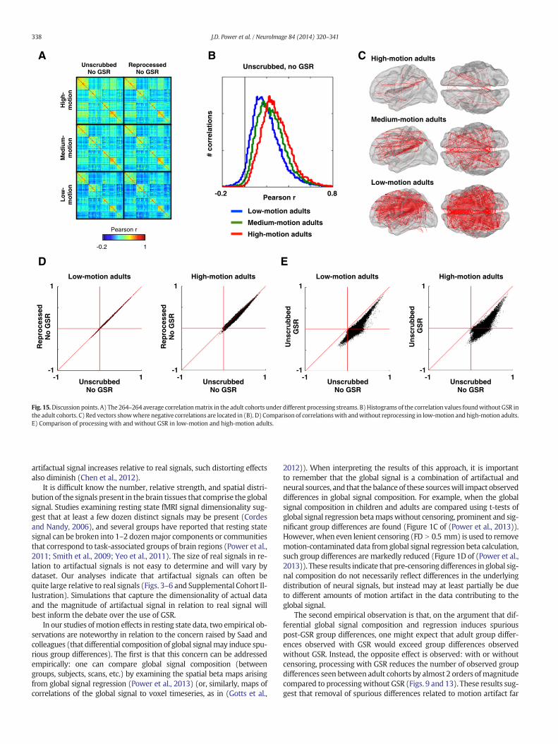
B

Pearson r 0.8-0.2

# co

rrel

atio

ns

Unscrubbed, no GSR

Low-motion adults

Medium-motion adults

High-motion adults

C

Low-motion adults

Medium-motion adults

High-motion adults

Low-motion adults High-motion adults Low-motion adults

-1

1

-1 1Unscrubbed

No GSR

Un

scru

bb

edG

SR

1

-1-1 1

Rep

roce

ssed

No

GS

R

High-motion adults1

-1-1 1

UnscrubbedNo GSR

Un

scru

bb

ed G

SR

UnscrubbedNo GSR

D E

A

-0.2 1

Pearson r

UnscrubbedNo GSR

ReprocessedNo GSR

Hig

h-

mo

tio

nM

ediu

m-

mo

tio

nL

ow

-m

oti

on

1

-1-1 1

Rep

roce

ssed

No

GS

R

UnscrubbedNo GSR

Fig. 15.Discussion points. A) The 264–264 average correlationmatrix in the adult cohorts under different processing streams. B)Histograms of the correlation values foundwithoutGSR inthe adult cohorts. C) Red vectors showwhere negative correlations are located in (B). D) Comparison of correlationswith andwithout reprocessing in low-motion and high-motion adults.E) Comparison of processing with and without GSR in low-motion and high-motion adults.


artifactual signal increases relative to real signals, such distorting effectsalso diminish (Chen et al., 2012).

It is difficult know the number, relative strength, and spatial distri-bution of the signals present in the brain tissues that comprise the globalsignal. Studies examining resting state fMRI signal dimensionality sug-gest that at least a few dozen distinct signals may be present (Cordesand Nandy, 2006), and several groups have reported that resting statesignal can be broken into 1–2 dozenmajor components or communitiesthat correspond to task-associated groups of brain regions (Power et al.,2011; Smith et al., 2009; Yeo et al., 2011). The size of real signals in re-lation to artifactual signals is not easy to determine and will vary bydataset. Our analyses indicate that artifactual signals can often bequite large relative to real signals (Figs. 3–6 and Supplemental Cohort Il-lustration). Simulations that capture the dimensionality of actual dataand the magnitude of artifactual signal in relation to real signal willbest inform the debate over the use of GSR.

In our studies ofmotion effects in resting state data, two empirical ob-servations are noteworthy in relation to the concern raised by Saad andcolleagues (that differential composition of global signalmay induce spu-rious group differences). The first is that this concern can be addressedempirically: one can compare global signal composition (betweengroups, subjects, scans, etc.) by examining the spatial beta maps arisingfrom global signal regression (Power et al., 2013) (or, similarly, maps ofcorrelations of the global signal to voxel timeseries, as in (Gotts et al.,

2012)). When interpreting the results of this approach, it is importantto remember that the global signal is a combination of artifactual andneural sources, and that the balance of these sourceswill impact observeddifferences in global signal composition. For example, when the globalsignal composition in children and adults are compared using t-tests ofglobal signal regression betamapswithout censoring, prominent and sig-nificant group differences are found (Figure 1C of (Power et al., 2013)).However, when even lenient censoring (FD N 0.5 mm) is used to removemotion-contaminated data from global signal regression beta calculation,such group differences are markedly reduced (Figure 1D of (Power et al.,2013)). These results indicate that pre-censoring differences in global sig-nal composition do not necessarily reflect differences in the underlyingdistribution of neural signals, but instead may at least partially be dueto different amounts of motion artifact in the data contributing to theglobal signal.

The second empirical observation is that, on the argument that dif-ferential global signal composition and regression induces spuriouspost-GSR group differences, one might expect that adult group differ-ences observed with GSR would exceed group differences observedwithout GSR. Instead, the opposite effect is observed: with or withoutcensoring, processing with GSR reduces the number of observed groupdifferences seen between adult cohorts by almost 2 orders ofmagnitudecompared to processingwithout GSR (Figs. 9 and 13). These results sug-gest that removal of spurious differences related to motion artifact far


outweighs spurious post-GSR distortions related to differential networkcomposition. This result is consistent with the recent report by Tyszkaand colleagues, wherein control versus autistic group differences weremuch smaller than motion-related effects within the same subjects(Tyszka et al., 2013).

Investigators considering global signal regression therefore face achoice. This paper has shown empirically that GSR is highly effectivein removing artifactual variance in RSFC data (Fig. 7), that adequatesubject-level motion artifact correction can be implemented with GSRin combination with censoring (Fig. 12), and that motion-relatedgroup differences are 1–2 orders of magnitude less with GSR than with-outGSR (Fig. 13). Recently published evidence shows thatGSR increasesthe resemblance of RSFC correlations to electrophysiological measures(Keller et al., 2013). Balanced against these benefits are the possible dis-tortions within networks and across groups highlighted by Murphyet al. and Saad et al. Our discussion confirms these concerns but empha-sizes that the relevance of these concerns to actual data is incompletelyestablished. On the whole, and certainly until other adequate methodsof artifact removal are developed, we find the empirical benefits to out-weigh the theoretical costs of GSR.

On detecting the influence of motion

This paper has used several approaches to quantify the influence ofmotion on BOLD signal and RSFC correlations. We wish to outline con-ceptually what, in our opinion, does and does not establish that adataset is free of artifactual influences related to motion.

Scrubbing analyses are useful because they can be applied at the in-dividual or the group level, and because they effectively characterizemotion-contaminated data. However, a censoring analysis that findsno distance-dependent artifact does not necessarily establish an ab-sence of distance-dependent artifact. Suppose, for instance, thatmotionwith FD N 0.2 mm corrupts data with a distance-dependent artifact. Ifdata with FD N 0.5 mm are replaced (by interpolation, by a meanvalue, etc.) and then a scrubbing analysis is performedwith a thresholdof FD N 0.5 mm, no distance-dependencewill be found. This result doesnot actually demonstrate that the data are free of artifact. If the scrub-bing threshold were lowered to FD N 0.4 or FD N 0.2 mm, distance-dependent artifact would be found. If the threshold were excessivelylowered into the range of normal data (e.g., FD N 0.1 mm), datawithoutmotion artifact would also be censored, diluting the characterization ofthe artifact-laden data. The central point is that outlying data (to be cen-sored) must be sensibly defined for the scrubbing analyses to be useful.

Table 2Summary of processing recommendations.

Why we do it

Censoring • Eliminates the influence of corrupted data• Conceptually and empirically most effectivimplemented throughout a processing stre

• Reduces dependence of correlations on moInterpolation • Reduces amplitude of artifactual signal spr

TRs during frequency filtering

Regression: global signal • Strongly reduces dependence of correlationMost effective at medium to long distanPositive relationships remain at short dcan be suppressed by censoring and int

• Eliminates post-motion influences on correOtherwise ~ 10 s post-motion influence

• Reduces shared non-motion artifactOtherwise need some other type of arti

• Increases RSFC correspondence to ECoGRegression: white matter, CSF • Modestly helpful at reducing artifactRegression: motion estimates • Modestly helpful at reducint artifact

• 24-parameter Volterra expansion increasinSuperior to our old 12-parameter regre

Because censoring analyses are threshold-dependent and can beperformed in ways that miss motion artifact, examination of QC-RSFCcorrelations is an important part of evaluating a dataset for influencesof motion. These analyses can only be employed across multiple scansor subjects, but their virtue is that no binarizing threshold is needed.For instance, in the example above, the scrubbing analysis using athreshold of FD N 0.5 mm might show no distance-dependence, butQC-RSFC correlations examined in the same dataset would reveal adistance-dependent effect. Even if a scrubbing threshold were sensiblydefined (e.g., FD N 0.2 mm in the present data), QC-RSFC correlationsmight reveal influences of smaller movements that are not practicallyaddressable or detectable by censoring analyses. It is for this reasonthat we focus on both scrubbing and QC-RSFC correlation analyses inthe present manuscript.

One other important consideration relates to the selection of QCmeasures for defining scrubbing or QC-RSFC correlation analyses. DV,since it is based on BOLD signal intensity, will differ across datasetsand processing strategies, and can be influenced by blurring kernelsize, frequency filter characteristics, sequence characteristics, etc. DVvalues may therefore not be comparable across datasets. FD measures(and other measures of absolute or relative displacement), on the faceof it, seem like they should be comparable across datasets. However,our experience with Human Connectome Project (HCP) data (see(Smith et al., 2013) for a description of the data) has altered this as-sumption. In contrast to the present data (acquired with TRs of 2.2–2.5 s), the HCP data are acquired with TRs of a few hundred millisec-onds. This shorter TR has the effect of dividing large movements intoseveral smaller movements, while simultaneously sampling effectslike head bobbing due to cardiac pulsations or respiration much morefrequently. The net effect is that, in the HCP data, DV traces exhibitsignal-to-noise ratios that are useful for identifying outlying datapoints,while FD traces are noisier and less useful in identifying outlyingtimepoints (unpublished observations). We raise these points to em-phasize that choosing an appropriate QC measure and utilizing it effec-tively requires attention to an individual dataset; simply taking athreshold or a QC measure from the literature without assessing itscharacteristics in the data at handmay result in uninformative analyses.

Overall summary

This paper aimed to expand knowledge about motion artifact in sev-eral ways. It illustrated the diversity of signal changes that motionproduces and pointed out some reasons why current subject-level

Possible drawbacks

e whenamtion

• Loss of data and possibly subjects• Unequal degrees of freedom across subjects

But can trim to equal size

ead into adjacent • Replacement data has synthetic characteristicsBetter than original characteristicsBut should probably not be treated as if it wereoriginal data (which is why we re-censor it)

s on motioncesistances, whicherpolationlationss

fact removal

• Removal of shared neural signal• If composed of few signals

Distorted correlation structurePossible misattributed group differences

gly usedssion

• Even large expansions (36 parameters) areinsufficient to remove motion artifact

• 12 degrees of freedom lost per order of expansion


regressions inadequately capturemotion-related variance. It placed tem-poral limits on the ability of motion to impact RSFC correlations. Itshowed that data improvements are partially cosmetic in terms of QCvalues and proposedmethods to link QCmeasures to significant changesin RSFC correlations. It proposed awithin-subject correction strategy thatgreatly reduces motion-related variance, and showed some conditionsunder which group-level correction is or is not necessary, or effective.Our current practices and recommendations are outlined in Table 2.

Limitations and future directions

The options for processing resting state data are numerous.We havepartially explored some parameter spaces corresponding to a subset ofpossibilities for data processing. Other possibilities remain to be ex-plored. A further limitation of this work is that only data acquiredusing a single sequence were examined. Other sequences may displaydifferent characteristics with regard to the magnitude, variety, and du-ration of motion-related effects. An additional limitation is that only asingle set of criteria was examined for forming temporal masks forreprocessing. It is possible that simple changes to our criteria mightyield easily obtainable improvements in control of motion artifact. An-other limitation is that only ‘functional connectivity processing’was ex-amined. It is possible that modifications earlier in the processing streamwould be more desirable, such as performing interpolation proceduresprior to slice-timing correction.

Post-hoc artifact reduction in resting state BOLD data is challenging.With advances such as short-TE or multi-band sequences (Bright andMurphy, 2013; Feinberg et al., 2010), future datasets will hopefully con-tainwithin themselves powerfulmeans of artifact avoidance and remov-al. Newer ICA-based techniques may prove successful in identifying andremoving artifactual influences. Novel treatments of realignment esti-mates may also prove more useful than current realignment-based cor-rections. We believe, however, that effective means for retrospectivecorrection of motion-related artifact are already available.

Acknowledgments

This work was funded by NIH F30 MH940322 (J.D.P.), NIHR21NS061144 (S.E.P.), a McDonnell Foundation Collaborative ActionAward (S.E.P.), Simons Foundation Award 95177 (S.E.P.), NIH5R01HD057076-03-S1 (B.L.S.), NIH R01HD057076 (B.L.S.), and NIHU54MH091657 (David Van Essen), NIH P30 NS048056 (A.Z.S) and P50NS006833 (A.Z.S.). This project was supported by the Intellectual and De-velopmental Disabilities Research Center atWashington University (NIH/NICHD P30 HD062171). Data were acquired with the support of NIH K12EY16336 (John Pruett). We thank Jessica Church, Joe Dubis, Eric Feczko,Katie Ihnen, Maital Neta, and Alecia Vogel for data contribution.

Conflict of interest statement

The authors have no conflicts of interest to report.

Appendix A. Supplementary data

Supplementary data to this article can be found online at http://dx.doi.org/10.1016/j.neuroimage.2013.08.048.

References

Anderson, J.S., Druzgal, T.J., Lopez-Larson, M., Jeong, E.-K., Desai, K., Yurgelun-Todd, D.,2011. Network anticorrelations, global regression, and phase-shifted soft tissue cor-rection. Hum. Brain Mapp. 32, 919–934.

Bright, M.G., Murphy, K., 2013. Removingmotion and physiological artifacts from intrinsicBOLD fluctuations using short echo data. NeuroImage 64, 526–537.

Carp, J., 2013. Optimizing the order of operations for movement scrubbing: comment onPower et al. NeuroImage 76, 436–438.

Chang, C., Glover, G.H., 2010. Time-frequency dynamics of resting-state brain connectivitymeasured with fMRI. NeuroImage 50, 81–98.

Chen, G., Chen, G., Xie, C., Ward, B.D., Li, W., Antuono, P., Li, S.-J., 2012. A method to deter-mine the necessity for global signal regression in resting-state fMRI studies. Magn.Reson. Med. 68, 1828–1835.

Cohen, A.L., Fair, D.A., Dosenbach, N.U.F., Miezin, F.M., Dierker, D., Van Essen, D.C.,Schlaggar, B.L., Petersen, S.E., 2008. Defining functional areas in individual humanbrains using resting functional connectivity MRI. NeuroImage 41, 45–57.

Cordes, D., Nandy, R.R., 2006. Estimation of the intrinsic dimensionality of fMRI data.NeuroImage 29, 145–154.

Feinberg, D.A., Moeller, S., Smith, S.M., Auerbach, E., Ramanna, S., Gunther, M., Glasser,M.F., Miller, K.L., Ugurbil, K., Yacoub, E., 2010. Multiplexed echo planar imaging forsub-second whole brain FMRI and fast diffusion imaging. PLoS One 5, e15710.

Fox, M.D., Zhang, D., Snyder, A.Z., Raichle, M.E., 2009. The global signal and observedanticorrelated resting state brain networks. J. Neurophysiol. 101, 3270–3283.

Friston, K.J., Williams, S., Howard, R., Frackowiak, R.S., Turner, R., 1996. Movement-relatedeffects in fMRI time-series. Magn. Reson. Med. 35, 346–355.

Gotts, S.J., Simmons, W.K., Milbury, L.A., Wallace, G.L., Cox, R.W., Martin, A., 2012. Frac-tionation of social brain circuits in autism spectrum disorders. Brain 135, 2711–2725.

Jo, H.J., Saad, Z.S., Simmons,W.K.,Milbury, L.A., Cox, R.W., 2010.Mapping sources of corre-lation in resting state FMRI, with artifact detection and removal. NeuroImage 52,571–582.

Keller, C.J., Bickel, S., Honey, C.J., Groppe, D.M., Entz, L., Craddock, R.C., Lado, F.A., Kelly, C.,Milham, M., Mehta, A.D., 2013. Neurophysiological investigation of spontaneous cor-related and anticorrelated fluctuations of the BOLD signal. J. Neurosci. 33, 6333–6342.

Kundu, P., Inati, S.J., Evans, J.W., Luh, W.-M., Bandettini, P.A., 2012. Differentiating BOLDand non-BOLD signals in fMRI time series using multi-echo EPI. NeuroImage 60,1759–1770.

Lemieux, L., Salek-Haddadi, A., Lund, T.E., Laufs, H., Carmichael, D., 2007. Modelling largemotion events in fMRI studies of patients with epilepsy. Magn. Reson. Imaging 25,894–901.

Lomb, N.R., 1976. Least-squares frequency analysis of unequally spaced data. Astrophys.Space Sci. 39, 447–462.

Mathias, A., Grond, F., Guardans, R., Seese, D., Canela, M., Diebner, H., 2004. Algorithms forspectral analysis of irregularly sampled time series. J. Stat. Softw. 11, 1–27.

Mowinckel, A.M., Espeseth, T., Westlye, L.T., 2012. Network-specific effects of age and in-scanner subjectmotion: a resting-state fMRI study of 238 healthy adults. NeuroImage63, 1364–1373.

Murphy, K., Birn, R.M., Handwerker, D.A., Jones, T.B., Bandettini, P.A., 2009. The impact ofglobal signal regression on resting state correlations: are anti-correlated networks in-troduced? NeuroImage 44, 893–905.

Power, J.D., Cohen, A.L., Nelson, S.M., Wig, G.S., Barnes, K.A., Church, J.A., Vogel, A.C.,Laumann, T.O., Miezin, F.M., Schlaggar, B.L., Petersen, S.E., 2011. Functional networkorganization of the human brain. Neuron 72, 665–678.

Power, J.D., Barnes, K.A., Snyder, A.Z., Schlaggar, B.L., Petersen, S.E., 2012. Spurious but sys-tematic correlations in functional connectivity MRI networks arise from subject mo-tion. NeuroImage 59, 2142–2154.

Power, J.D., Barnes, K.A., Snyder, A.Z., Schlaggar, B.L., Petersen, S.E., 2013. Steps toward op-timizing motion artifact removal in functional connectivity MRI; a reply to Carp.NeuroImage 76, 439–441.

Saad, Z.S., Gotts, S.J., Murphy, K., Chen, G., Jo, H.J., Martin, A., Cox, R.W., 2012. Trouble atrest: how correlation patterns and group differences become distorted after globalsignal regression. Brain Connect. 2, 25–32.

Satterthwaite, T.D., Wolf, D.H., Loughead, J., Ruparel, K., Elliott, M.A., Hakonarson, H., Gur,R.C., Gur, R.E., 2012. Impact of in-scanner head motion on multiple measures of func-tional connectivity: relevance for studies of neurodevelopment in youth. NeuroImage60, 623–632.

Satterthwaite, T.D., Elliott, M.A., Gerraty, R.T., Ruparel, K., Loughead, J., Calkins, M.E.,Eickhoff, S.B., Hakonarson, H., Gur, R.C., Gur, R.E., Wolf, D.H., 2013. An improvedframework for confound regression and filtering for control of motion artifactin the preprocessing of resting-state functional connectivity data. NeuroImage64, 240–256.

Schölvinck, M.L., Maier, A., Ye, F.Q., Duyn, J.H., Leopold, D.A., 2010. Neural basis of globalresting-state fMRI activity. Proc. Natl. Acad. Sci. U. S. A. 107, 10238–10243.

Shulman, G.L., Pope, D.L.W., Astafiev, S.V., McAvoy, M.P., Snyder, A.Z., Corbetta, M., 2010.Right hemisphere dominance during spatial selective attention and target detectionoccurs outside the dorsal frontoparietal network. J. Neurosci. 30, 3640–3651.

Smith, S.M., Fox, P.T., Miller, K.L., Glahn, D.C., Fox, P.M., Mackay, C.E., Filippini, N., Watkins,K.E., Toro, R., Laird, A.R., Beckmann, C.F., 2009. Correspondence of the brain's functionalarchitecture during activation and rest. Proc. Natl. Acad. Sci. U. S. A. 106, 13040–13045.

Smith, S.M., Miller, K.L., Moeller, S., Xu, J., Auerbach, E.J., Woolrich, M.W., Beckmann, C.F.,Jenkinson, M., Andersson, J., Glasser, M.F., Van Essen, D.C., Feinberg, D.A., Yacoub, E.S.,Ugurbil, K., 2012. Temporally-independent functional modes of spontaneous brainactivity. Proc. Natl. Acad. Sci. U. S. A. 109, 3131–3136.

Smith, S.M., Beckmann, C.F., Andersson, J., Auerbach, E.J., Bijsterbosch, J., Douaud, G.,Duff, E., Feinberg, D.A., Griffanti, L., Harms, M.P., Kelly, M., Laumann, T., Miller,K.L., Moeller, S., Petersen, S., Power, J., Salimi-Khorshidi, G., Snyder, A.Z., Vu,A.T., Woolrich, M.W., Xu, J., Yacoub, E., Uğurbil, K., Van Essen, D.C., Glasser, M.F.,Consortium, W.U.-M.H., 2013. Resting-state fMRI in the human connectome pro-ject. NeuroImage 80, 144–168.

Smyser, C.D., Inder, T.E., Shimony, J.S., Hill, J.E., Degnan, A.J., Snyder, A.Z., Neil, J.J., 2010.Longitudinal analysis of neural network development in preterm infants. Cereb. Cor-tex 20, 2852–2862.

Tyszka, J.M., Kennedy, D.P., Paul, L.K., Adolphs, R., 2013. Largely typical patterns ofresting-state functional connectivity in high-functioning adults with autism.Cereb. Cortex (in press).



http://refhub.elsevier.com/S1053-8119(13)00911-7/rf0005














































































Van Dijk, K.R.A., Hedden, T., Venkataraman, A., Evans, K.C., Lazar, S.W., Buckner, R.L., 2010.Intrinsic functional connectivity as a tool for human connectomics: theory, proper-ties, and optimization. J. Neurophysiol. 103, 297–321.

Van Dijk, K.R.A., Sabuncu, M.R., Buckner, R.L., 2012. The influence of head motion on in-trinsic functional connectivity MRI. NeuroImage 59, 431–438.

Weissenbacher, A., Kasess, C., Gerstl, F., Lanzenberger, R., Moser, E., Windischberger, C.,2009. Correlations and anticorrelations in resting-state functional connectivity MRI:a quantitative comparison of preprocessing strategies. NeuroImage 47, 1408–1416.

Yan, C.-G., Cheung, B., Kelly, C., Colcombe, S., Craddock, R.C., Di Martino, A., Li, Q., Zuo, X.-N., Castellanos, F.X., Milham,M.P., 2013. A comprehensive assessment of regional var-iation in the impact of head micromovements on functional connectomics.NeuroImage 76C, 183–201.

Yeo, B.T.T., Krienen, F.M., Sepulcre, J., Sabuncu, M.R., Lashkari, D., Hollinshead, M.,Roffman, J.L., Smoller, J.W., Zöllei, L., Polimeni, J.R., Fischl, B., Liu, H., Buckner, R.L.,2011. The organization of the human cerebral cortex estimated by intrinsic functionalconnectivity. J. Neurophysiol. 106, 1125–1165.












methods to detect, characterize, and remove motion ...cogns.northwestern.edu/cbmg/motion in resting...

Documents