methods for sugarcane harvest detection using polarimetric sar · sugarcane, the growth period of...

Methods for sugarcane harvest detection using polarimetric

SAR

by

MICHAEL DANIEL PORTNOI

Thesis presented in fulfilment of the requirements for the degree of

Master of Geo-Informatics in the Faculty of Science at

Stellenbosch University

Supervisor: Dr Jaco Kemp

Co-supervisor: Dr Pierre Todoroff

March 2017

DECLARATION

By submitting this report electronically, I declare that the entirety of the work contained therein

is my own, original work, that I am the sole author thereof (save to the extent explicitly

otherwise stated), that reproduction and publication thereof by Stellenbosch University will not

infringe any third party rights and that I have not previously, in its entirety or in part, submitted it

for obtaining any qualification.

Date: March 2017

Copyright © 2017 Stellenbosch University

All rights reserved

Stellenbosch University https://scholar.sun.ac.za

ii

SUMMARY

Remote sensing has long been used as a method for crop harvest monitoring and harvest

classification. Harvest monitoring is necessary for the planning of and prompting of effective

agricultural practices. Traditionally sugarcane harvest monitoring and classification within the

realm of remote sensing is performed with the use of optical data. However, when monitoring

sugarcane, the growth period of the crop requires a complete set of multi-temporal image

acquisitions throughout the year. Due to the limitations associated with optical sensors, the use

of all weather, daylight independent Synthetic Aperture Radar (SAR) sensors is required. The

added polarimetric information associated with fully polarimetric SAR sensors result in complex

datasets which are expensive to acquire. It is therefore important to assess the benefits of using a

fully polarimetric dataset for sugarcane harvest monitoring as opposed to a dual polarimetric

dataset. The dual polarimetric dataset which is less complex in nature and can be acquired at a

fee much less than that of the fully polarimetric dataset. This thesis undertakes the task of

identifying the value of fully polarimetric data for sugarcane harvest identification and

classification. Two main experiments were designed in order to complete the task. The

experiments make use of fully polarimetric RADARSAT-2 C-band imagery covering the

southern part of Rèunion Island.

Experiment 1 made use of a multi temporal single feature differencing technique for sugarcane

harvest identification. Polarimetric decompositions were extracted from the fully polarimetric

data and used along with the inherent SAR features. The accuracy with which each SAR feature

was able to predict the sugarcane harvest date for each field was assessed. The polarimetric

decompositions were superior in classification accuracy to the inherent SAR features. The Van

Zyl volume decomposition component achieved an accuracy of 88.33% whereas the inherent

SAR backscatter feature (HV) achieved an accuracy of 80%. Hereby displaying the value of the

added information associated with fully polarimetric SAR data. The SAR backscatter channels

did not achieve accuracies as high as the polarimetric features but did display promise for single

feature sugarcane harvest identification when using only a dual polarimetric dataset.

Experiment 2 assessed six different machine learning classifiers, applied to single-date, dual- and

fully polarized imagery, to determine appropriate combinations of machine learning classifier

and SAR features. Polarimetric decompositions were extracted from the fully polarimetric data

and mean texture measures were then calculated for all SAR features for both the dual- and full

polatrimetric data. A multi-tiered feature reduction method was undertaken in order to reduce

dataset dimensionality for the dual- and fully polarised datasets. In general, the reduction in

features resulted in improved accuracies. The best sugarcane harvest accuracy was achieved


iii

using the Maximum likelihood classifier using on the HV and VV backscatter channels

(96.18%).

The results from Experiments 1 and 2 indicate that SAR C-band data is suitable for sugarcane

harvest monitoring and mapping in a tropical region where optical data have limitations

associated with cloud cover and large amounts of moisture in the atmosphere. With the

availability of dual polarised Sentinel-1 SAR data, future research should be focussed on the use

of a dual polarimetric sugarcane harvest monitoring tool and should be extended to focus not

only on sugarcane but other crops which contribute largely to the agriculture and economic

sectors

KEY WORDS

Harvest identification, harvest classification, SAR, RADARSAT-2, machine learning, feature

reduction, fully polarimetric, dual polarimetric.


iv

OPSOMMING

Afstandswaarneming word lankal reeds gebruik as ‘n metode in die monitering van die oes van

gewasse asook vir oes-klassifikasie. Oes-monitering is nodig vir die beplanning en stimulering

van effektiewe landboupraktyke. Tradisioneel word suikerriet oes-monitering en klassifisering,

binne die raamwerk van afstandswaarneming, uitgevoer met die gebruik van optiese data. Tog,

met die monitering van suikerriet, vereis die groeiperiode van die gewas ‘n volledige stel multi-

temporale beeldverwerwings dwarsdeur die jaar. As gevolg van die beperkings geassosieer met

optiese sensors, word die gebruik van daglig onafhanklike sintetiese gaatjie radar sensors, eerder

bekend as Sintetiese Apertuur Radar (SAR) sensors, vir gebruik in alle weersomstandighede,

vereis. Die bykomende polarimetriese informasie geassosieer met ten volle gepolarimetriese

SAR sensors lei tot komplekse datastelle wat duur is om aan te skaf. Dit is daarom belangrik om

die voordele van die gebruik van ‘n ten volle gepolarimetriese datastel vir suikerriet oes-

monitering in teenstelling met ‘n tweeledige polarimetriese datastel wat minder kompleks van

aard is en teen ‘n fooi veel minder as dié van die ten volle gepolarimetriese datastel verkry kan

word, te evalueer. Hierdie tesis onderneem die taak van die identifisering van die waarde van ten

volle gepolarimetriese data vir suikerriet oes-identifikasie en -klassifikasie. Twee hoof-

eksperimente is ontwerp om die taak te voltooi. Die eksperimente gebruik ten volle

gepolarimetriese RADARSAT-2 C-band beelde wat die suidelike deel van Reunion-eiland dek.

Met eksperiment 1 is gebruik gemaak van 'n multi-temporale enkelkenmerk differensie- tegniek

vir suikerriet oes-identifisering. Polarimetriese ontledings is uit die ten volle gepolarimetriese

data geneem en saam met die inherente SAR kenmerke gebruik. Die akkuraatheid waarmee elke

SAR kenmerk in staat was om die suikerriet oes-datum vir elke veld te voorspel, is geëvalueer.

Die polarimetriese ontledings was beter in klassifikasie- akkuraatheid as die inherente SAR

kenmerke. Hiermee word die waarde van die bykomende inligting geassosieer met ten volle

gepolarimetriese SAR data, geopenbaar. Die SAR teruguitsaaiingskanale het nie akkuraathede so

hoog soos die polarimetriese kenmerke bereik nie, maar het belofte getoon vir enkelkenmerk

suikerriet oes-identifikasie wanneer slegs van 'n tweeledige polarimetriese datastel gebruik

gemaak word.

Met eksperiment 2 is ses verskillende masjien-leer klassifiseerders, toegepas op enkeldatum,

tweeledige en ten volle gepolariseerde beelde, geëvalueer om toepaslike kombinasies van

masjien-leer klassifiseerder en SAR kenmerke te bepaal. Polarimetriese ontledings is geneem uit

die ten volle gepolarimetriese data en beteken dat tekstuur afmetings toe bereken is vir alle SAR

kenmerke vir beide die tweeledige- en ten volle gepolarimetriese data. 'n Multi-reeks

kenmerkreduksie-metode is onderneem om datasteldimensionaliteit te verminder vir die


v

tweeledige- en ten volle gepolariseerde datastelle. Oor die algemeen het die redusering van

kenmerke verbeterde akkuraatheid tot gevolg gehad. Die beste suikerriet oes-akkuraatheid is

behaal deur die Maksimum waarskynlikheid klassifiseerder met behulp van die HV en VV

teruguitsaaiingskanale (96,18%) te gebruik.

Die resultate van eksperimente 1 en 2 dui daarop dat SAR C-band data geskik is vir suikerriet

oes- monitering en kartering in 'n tropiese streek waar optiese data beperkings toon wat

geassosieer word met wolkbedekking en groot hoeveelhede vog in die atmosfeer. Met die

beskikbaarheid van tweeledige gepolariseerde Sentinel-1 SAR data, behoort toekomstige

navorsing gefokus te wees op die gebruik van 'n tweeledige polarimetriese suikerriet oes-

moniteringshulpmiddel en behoort dit uitgebrei te word om te fokus nie net op suikerriet nie,

maar ook ander gewasse wat grootliks bydra tot die landbou- en ekonomiese sektore.

TREFWOORDE

Oes-identifikasie, oes-klassifikasie, SAR, RADARSAT-2, masjien-leer, kenmerkreduksie, ten

volle gepolarimetriese, tweeledige polarimetriese


vi

ACKNOWLEDGEMENTS

I would sincerely like to thank:

Dr Jaco Kemp for his insight, guidance, support throughout the duration of the project

and for affording me the opportunity to travel to Rèunion Island;

My co-supervisor Dr Pierre Todoroff and CIRAD for accommodating me for my two

month stay on Rèunion Island;

My parents for affording me the privilege to study at the University of Stellenbosch and

for their constant support, love and motivation;

The National Research Foundation (NRF) for their generous funding throughout the two

years of this degree;

SEAS-OI for providing me with my satellite image data;

Dr Rose Masha for the grammar editing of this thesis;

The Centre for Geographical Analysis (CGA) and Gerhard Myburgh for the SLICE

software.


vii

CONTENTS

DECLARATION ...................................................................................................... i

SUMMARY .............................................................................................................. ii

OPSOMMING ........................................................................................................ iv

ACKNOWLEDGEMENTS ................................................................................... vi

CONTENTS ........................................................................................................... vii

TABLES .................................................................................................................. xi

FIGURES ............................................................................................................... xii

ACRONYMS AND ABBREVIATIONS ............................................................ xiv

CHAPTER 1: INTRODUCTION ....................................................................... 1

1.1 BACKGROUND TO THE STUDY ............................................................................. 1

1.2 PROBLEM STATEMENT........................................................................................... 2

1.3 RESEARCH AIM AND OBJECTIVES ..................................................................... 4

1.4 METHODOLOGY AND RESEARCH DESIGN ....................................................... 5

1.5 STUDY SITE ................................................................................................................. 7

1.6 STRUCTURE OF THESIS ........................................................................................ 10

CHAPTER 2: LITERATURE REVIEW ......................................................... 11

2.1 REMOTE SENSING FOR LAND COVER CLASSIFICATION AND

AGRICULTURE ..................................................................................................................... 11

2.2 SAR INTRODUCTION .............................................................................................. 13

2.2.1 SAR pre-processing ............................................................................................. 14

2.2.1.1 Terrain correction and geocoding ..................................................................... 14

2.2.1.2 Radiometric calibration ..................................................................................... 16

2.2.1.3 SAR filtering ..................................................................................................... 17

2.2.2 SAR backscatter .................................................................................................. 18

2.2.2.1 Factors affecting SAR backscatter .................................................................... 18

2.2.3 SAR data structure .............................................................................................. 20

2.2.4 SAR decompositions ............................................................................................ 21

2.3 IMAGE CLASSIFICATION USING SAR ............................................................... 23

2.3.1 Object vs pixel based classifications .................................................................. 23

2.3.2 Feature selection .................................................................................................. 24

2.3.3 Classification algorithms .................................................................................... 25


viii

2.4 SHEWHART INDIVIDUAL CONTROL CHARTS ............................................... 28

2.5 SYNTHETIC APERTURE RADAR APPLICATIONS IN AGRICULTURE ..... 30

2.5.1 General SAR in agriculture ................................................................................ 30

2.5.2 SAR in harvest monitoring ................................................................................. 32

2.5.3 SAR image classification in agriculture ............................................................ 33

2.5.4 SAR in sugarcane monitoring ............................................................................ 35

2.5.5 Application of Remote Sensing to sugarcane on Rèunion ............................... 36

2.5.6 Key findings in literature .................................................................................... 37

CHAPTER 3: MATERIALS AND METHODS .............................................. 38

3.1 DATA ACQUISTION ................................................................................................. 38

3.2 DATA PREPERATION AND MANIPULATION................................................... 40

3.2.1 Pre-processing the backscatter bands ............................................................... 41

3.2.1.1 Filtering of backscatter bands for Objective 2 .................................................. 42

3.2.1.2 Filtering of backscatter bands for Objective 3 .................................................. 42

3.2.2 Pre-processing the coherency matrix (T3) ........................................................ 42

3.2.3 Ground truth database ....................................................................................... 43

3.2.4 Feature extraction ............................................................................................... 44

3.2.4.1 Polarimetric Information ................................................................................... 44

3.2.4.2 Image texture ..................................................................................................... 45

3.2.4.3 Summary of image layers .................................................................................. 46

3.3 EXPERIMENT 1: SINGLE FEATURE HARVEST MONITORING .................. 47

3.3.1 Shewhart individual control charts ................................................................... 48

3.3.2 Shewhart individual control charts accuracy assessment ............................... 50

3.4 EXPERIMENT 2: SINGLE IMAGE HARVEST CLASSIFICATION................. 50

3.4.1 Feature selection .................................................................................................. 50

3.4.1.1 Exploratory Factor Analysis.............................................................................. 51

3.4.1.2 One-way ANOVA ............................................................................................. 52

3.4.2 Image classification ............................................................................................. 53

3.4.3 Classification accuracy ....................................................................................... 54

CHAPTER 4: RESULTS AND DISCUSSION EXPERIMENT 1 ................. 55

4.1 Shewhart individual control charts based on mean value ....................................... 55

4.1.1 Harvest detection ................................................................................................. 56

4.1.2 Harvest monitoring ............................................................................................. 57

4.2 Improving Shewhart individual control chart accuracy ......................................... 60

4.2.1 Comparison between mean and median field values ....................................... 60


ix

4.2.2 Comparison of differencing and ratio MR calculation .................................... 61

4.2.3 Appropriate size of multi-temporal dataset ...................................................... 62

4.3 Points to highlight from Experiment 1 ...................................................................... 64

CHAPTER 5: RESULTS AND DISCUSSION EXPERIMENT 2 ................. 65

5.1 Feature selection .......................................................................................................... 65

5.1.1 Fully polarimetric Exploratory Factor Analysis (EFA) results ...................... 66

5.1.2 Fully polarimetric ANOVA results .................................................................... 66

5.1.3 Dual polarimetric Exploratory Factor Analysis (EFA) results ....................... 68

5.1.4 Dual polarimetric ANOVA results .................................................................... 69

5.1.5 Datasets for image classification ........................................................................ 70

5.2 Fully polarimetric image classification ..................................................................... 71

5.2.1 Accuracy using all features ................................................................................. 71

5.2.2 Factor Analysis-reduced features ...................................................................... 73

5.2.3 ANOVA-reduced features .................................................................................. 74

5.2.4 Fully polarimetric classification comparison .................................................... 76

5.3 Dual polarimetric image classification ...................................................................... 78

5.3.1 Dual polarimetric classification using all features ........................................... 78

5.3.2 Dual polarimetric classification post EFA ........................................................ 80

5.3.3 Dual polarimetric classification post ANOVA.................................................. 80

5.3.4 Dual polarimetric HV and VV ........................................................................... 82

5.3.5 Dual polarimetric classification comparison .................................................... 83

5.4 Fully polarimetric vs dual polarimetric image classification .................................. 85

5.5 Points to highlight from Experiment 2 ...................................................................... 87

CHAPTER 6: CONCLUSION .......................................................................... 88

6.1 SYNTHESIS AND FINDINGS OF THE STUDY .................................................... 88

6.1.1 Experiment 1 ........................................................................................................ 88

6.1.2 Experiment 2 ........................................................................................................ 89

6.2 CONTEXTUALIZING THE FINDINGS ................................................................. 90

6.3 CONTRIBUTION AND NOVELTY ......................................................................... 92

6.4 LIMITATIONS ........................................................................................................... 93

6.5 RECOMMENDATIONS ............................................................................................ 94

6.5.1 Operational recommendations ........................................................................... 94

6.5.2 Research recommendations ................................................................................ 95

6.6 CONCLUDING REMARKS ...................................................................................... 96

6.7 CONTINUATION OF THIS RESEARCH............................................................... 97


x

REFERENCES ...................................................................................................... 98


xi

TABLES

Table 3.1 RADARSAT-2 time series image number and acquisition date. ................................ 39

Table 3.2 Harvest status identification method with metadata describing nature of information

captured. .................................................................................................................... 39

Table 4.1 Harvest monitoring confusion matrix for Freeman-Durden Volume scattering

component displaying overall accuracy, error of commission and error of omission

................................................................................................................................... 58

Table 4.2 Overall accuracies for harvest detection and identification, Kappa values and errors of

commission and omission for each of the 6 best performing features ...................... 59

Table 4.3 Harvest identification accuracy for selected features based on the number of images

used ............................................................................................................................ 63

Table 5.1 Top 10 fully polarimetric features selected by ANOVA; the features retained are

marked with an asterisk ............................................................................................. 67

Table 5.2 Top 10 dual polarimetric features selected by ANOVA, the features retained are

marked with an asterisk ............................................................................................. 69

Table 5.3 Feature reduced datasets for image classification and the corresponding sections in

the text where the results for each are presented. ...................................................... 71

Table 5.4 Results for fully polarimetric image classification using all features ......................... 71

Table 5.6 Results for fully polarimetric image classification using a feature dataset reduced by

ANOVA ..................................................................................................................... 75

Table 5.7 Results for dual polarimetric image classification using all features .......................... 78

Table 5.8 Results for dual polarimetric image classification using a feature dataset reduced by

ANOVA ..................................................................................................................... 81

Table 5.9 Results for dual polarimetric image classification using a feature dataset containing

only HV and VV backscatter channels ...................................................................... 82


xii

FIGURES

Figure 1.1 Research design ........................................................................................................... 6

Figure 1.2 The study site highlighted by the red box on Rèunion Island, located East of

Madagascar in the Indian Ocean. ................................................................................ 8

Figure 1.3 Sugarcane fields, green points, northeast of St. Pierre ................................................ 9

Figure 2.1 (a) Transmitted or incident signal from SAR sensor. (b) The backscattered signal

following interaction with targets on the Earth’s surface. ......................................... 14

Figure 2.2 Radar foreshortening .................................................................................................. 15

Figure 2.3 Radar layover ............................................................................................................. 16

Figure 2.4 Shewhart individual control chart for a manufacturing process. ............................... 29

Figure 3.1 Aerial photograph showing (a) sugarcane field with homogeneous harvest status and

(b) sugarcane field with heterogeneous/partial harvest status. .................................. 40

Figure 3.2 Pre-processing workflow for preparation of RADARSAT-2 imagery. ..................... 41

Figure 3.3 Shewhart Individual Control chart indicating control limits and image number where

control limits are exceeded for field ID 2132 using the Freeman-Durden Volume

scattering feature. ...................................................................................................... 49

Figure 3.4 An example of a Scree plot and the natural bend in the curve indicated with a red

box. ............................................................................................................................ 52

Figure 4.1 SAR features and their accuracies for sugarcane harvest detection .......................... 56

Figure 4.2 Averaged errors of commission and omission for each of the 6 best performing

features ...................................................................................................................... 60

Figure 4.3 Visual representation of Mean vs Median accuracy for sugarcane harvest

identification. ............................................................................................................. 61

Figure 4.4 Overall accuracy comparing between Differencing and Ratio techniques for MR

calculation. ................................................................................................................ 62

Figure 4.5 Visual increase in accuracy for increase in dataset size for sugarcane harvest

detection. ................................................................................................................... 63

Figure 5.1 Scree indicating factor scores post EFA for the fully polarimetric dataset ............... 66

Figure 5.2 Scree indicating factor scores post EFA for the fully polarimetric dataset ............... 68

Figure 5.3 Box plots representing overall classification accuracy for fully polarimetric data

using all features ........................................................................................................ 72

Figure 5.4 Boxplots representing overall classification accuracy for fully polarimetric data

using a feature dataset reduced by EFA ................................................................. 74


xiii

Figure 5.5 Box plots representing overall classification accuracy for fully polarimetric data

using a feature dataset reduced by ANOVA .......................................................... 76

Figure 5.6 Comparison of classification accuracy after each stage of feature reduction for each

classification algorithm using the fully polarimetric dataset. .................................... 77

Figure 5.7 Comparison of Kappa values after each stage of feature reduction for each

classification algorithm using the fully polarimetric dataset ..................................... 77

Figure 5.9 Box plots representing overall classification accuracy for dual polarimetric data

using a feature dataset reduced by ANOVA .......................................................... 81

Figure 5.10 Box plots representing overall classification accuracy for dual polarimetric data

using a feature dataset containing only HV and VV backscatter channels ............... 83

Figure 5.12 Comparison of the Kappa value after each stage of feature reduction for each

classification algorithm using the dual polarimetric dataset. .................................... 85

Figure 5.13 Comparison of classification accuracy between fully polarimetric, dual

polarimetric and HV and VV only datasets at the final stage of feature reduction for

each classification algorithm ..................................................................................... 86


xiv

ACRONYMS AND ABBREVIATIONS

ACP

ANOVA

CIRAD

CSA

DEM

DT

EFA

GIS

GLCM

GLDV

African Caribbean and Pacific

Analysis of Variance

Centre de coopération internationale en recherche agronomique pour le

dévelopement

Canadian Space Agency

Digital elevation model

Decision Trees

Exploratory Factor Analysis

Geographical information systems

Grey level co-occurrence matrix

Grey level difference vector

GPS

KNN

LCL

ML

MR

OA

OBIA

PolSAR

RT

Global positioning systems

K-Nearest Neighbour

Lower confidence limit

Maximum Likelihood

Moving range

Overall accuracy

Object based image analysis

Polarimetric SAR

Random Trees

RS

SAR

SVM

SEAS-OI

UCL

Remote Sensing

Synthetic Aperture Radar

Support Vector Machines

Surveillance de l'Environnement Assistée par Satellite pour l'Ocean

Indien

Upper confidence limit


1

CHAPTER 1: INTRODUCTION

This chapter serves as an introduction to the thesis, providing background information to

contextualise the study. The problem formulation, aim and objectives, methodology and a

research design indicating the structure of the thesis are outlined.

1.1 BACKGROUND TO THE STUDY

The world currently has a population of approximately 7 billion people, with this number

expected to exceed 9 billion by mid-21st century (Miccoli, Finnuci & Munro 2016). Developing

countries are predicted to grow at a more rapid rate than developed countries, whose populations

are expected to decrease (Miccoli, Finnuci & Munro 2016). With the expected population

increase, urban expansion is an inevitability in developing countries, hereby reducing the

available arable land to be used for agricultural activities. With most facets of food production

having roots in agriculture, concerns relating to food security will increase, especially in

developing countries (Shi et al. 2014).

The sugarcane industry is a large provider of products to global markets. The crop is currently

viewed as the world’s largest crop by production quantity (FAOSTATS 2016). Sugarcane is

most commonly used for the production of raw sugar and has recently emerged as a major

producer sugarcane-ethanol which is a widely used biofuel (Tsao et al. 2012). The expanding

global population directly influences sugarcane production. Recent figures show that sugarcane

productivity in developing countries, namely, African, Caribbean and Pacific (ACP) countries is

much lower than expected and even lower when compared to more developed, industrialised

sugarcane producers (FAOSTATS 2016). These industrialised countries make use of precision

farming for improved yield. However, the technologies associated with the practice of precision

farming are not always available in developing countries.

The importance of sugarcane for developing states is highlighted by the case of the tropical

island of La Rèunion. The agricultural sector is dominated by sugarcane production, with the

crop comprising approximately 80% of all acreages associated with agriculture (FAOSTATS

2016) and is estimated to provide a source of income for 5000 small-scale subsistence farmers

with holdings generally less than 5 hectares (Lejars & Siegmund 2004). The importance of the

crop is further highlighted in that it provides 22% of the island’s electricity (Lejars & Siegmund

2004). Due to the islands’ predominately-steep topography, mechanised harvesters are unable to

function in most areas; sugarcane crops are therefore planted and harvested manually. The main

reason for the harvest occurring manually is that the mechanised harvesters are not freely

available to small-scale farmers due to the costs involved. Baghdadi et al. (2009) cite the


2

importance of developing cost-efficient, easily accessible sugarcane monitoring applications for

these small-scale farmers in order to prompt effective farming practices which will, in turn,

improve sugarcane yield.

Remote Sensing (RS), more specifically Synthetic Aperture Radar (SAR), is an efficient

technology for acquiring data for use in land cover analysis and classification. SAR provides the

ability to acquire a complete dataset, which is often not possible when using optical imagery due

to limitations associated with cloud clover. This is supported by the increase in the availability of

SAR imagery as well as the rapid development of technology leading to cost and time efficient

image acquisition. The classification of land cover as a tool for quantifying and monitoring

changes associated with the Earths’ system processes is identified in scientific communities as a

key element in the study of global change (Henderson-Sellers & Pitman 1992).

As an extension of land cover mapping, crop mapping is important for agricultural and economic

applications. The monitoring and surveying of existing crops allow for the production of crop

maps, which play a major role in identifying and discriminating between different crop types

(Mahmoud et al. 2011; Singh et al. 2002), crop distributions and in predicting future crop yields

(Benedetti & Rossini 1991; Lobell et al. 2003). Agricultural targets are very dynamic throughout

the growing season, therefore remote sensing is an attractive approach for mapping and

monitoring agicultural applications. Acquiring timely information relating to the spatial and

structural distribution of crops as well as optimum conditions for these crops is important for

governments at various levels. This information aids in effective decision making to diminish

food insecurity risks (Shi et al. 2014). The large acreages associated with modern day

agricultural applications have exhausted the ability of traditional field-based surveying

techniques to be effective in mapping and monitoring resources. They are also time consuming

and can become costly depending on the number and type of observations required (Engelbrecht,

Kemp & Inggs 2013).

1.2 PROBLEM STATEMENT

Harvest monitoring and detection within the realm of remote sensing has, traditionally, been

performed with the use of optical data. However, when monitoring sugarcane, the growth period

of the crop requires a complete set of multi-temporal image acquisitions throughout the year.

Due to the limitations associated with optical sensors, the use of all weather, daylight

independent SAR sensors is required. The microwave wavelength at which SAR sensors operate

allows for image acquisitions to take place when weather conditions do not allow for the

traditional optical sensors to capture images (McCandless & Jackson 2004). This is especially

important in tropical regions where cloud cover is eminent and sugarcane cultivation is important


3

as it is often a crop that provides a source of food, income and electricity for those residing in

tropical regions.

Sugarcane is the most important crop for the tropical island of La Rèunion, occupying 25 000

hectares of the approximately 31 500 hectares (80%) of primary agricultural land with a yield of

1.9 million tons per year (FAOSTATS 2016). The majority of sugarcane growers on the island

are small-scale farmers. The crop provides a livelihood for most of the population as well as

providing the basis for the development of the agro-industry (Lejars & Siegmund 2004). Lejars

and Siegmund (2004) suggest that the sugarcane mills need to produce an average of 2.5 million

tons of cane a year and increase coverage of the sugarcane growing area to 30 000 hectares.

However, with the constant increase in population size, the sizes of towns are increasing and

arable land is being diminished.

The monitoring and identification of the sugarcane harvest is necessary for the planning of and

prompting of effective agricultural practices. These include optimized cutter development,

transport operations, efficiency of factories and better estimation of the final yield (Baghdadi et

al. 2010).

The use of SAR for sugarcane monitoring applications has been previously investigated

(Baghdadi et al. 2009; Baghdadi et al. 2010). These studies have experimented with the use of

dual-polarised C-, X-and L-band data. Baghdadi et al. (2009) aimed at identifying the best radar

configurations for sugarcane harvest monitoring. The sensitivity of wavelength, incidence

angles, and polarization were analysed in relation to sugarcane crop height with particular

emphasis on harvest identification. Baghdadi et al. (2010) performed an extension of the

previous study by incorporating a multi-temporal X-band dataset not previously available.

While previous studies investigated the use of fully polarimetric SAR data (Turkar & Rao 2011;

Lopez-Sanchez, Cloude & Ballester-Berman 2014; Furtado, Silva & Nova 2016). The use of

fully polarimetric SAR data, including polarimetric decompositions, has not been sufficiently

investigated. In addition to this, the recent launch of the Sentinal-1 sensors under the Copernicus

program, dual-polarised C-band SAR data is becoming more freely available and hereby presents

the need to test a dual polarised scenario to be used for sugarcane harvest monitoring and

mapping.

This study aims to assess sugarcane harvest monitoring and detection using fully polarimetric C-

band data as well as make comparisons with C-band dual polarised data. This will allow for

assessing the value of each of the datasets for sugarcane harvest monitoring and draw

conclusions based on the value of the added polarimetric information available. The added

information available when using fully polarimetric data requires further processing to extract


4

the full potential of the data. Extracting the full potential of the fully polarimetric data can

become costly and time consuming.

The need for comparison between fully polarimetric SAR data and dual polarimetric data for

sugarcane harvest monitoring to be investigated poses in the following questions:

1. What is the effectiveness of a multi-temporal single feature differencing method for

harvest monitoring?

2. What is the appropriate size of the multi-temporal dataset required for achieving peak

harvest detection accuracy?

3. What is the effect of feature selection on classification accuracy for harvested and

unharvested sugarcane fields on a single image for both a fully polarimetric and a dual

polarimetric case?

4. Which classification algorithm is best able to identify harvested and unharvested

sugarcane fields on a single image using a fully polarimetric and a dual polarimetric

dataset?

5. What is the added value of using a fully polarimetric dataset in comparison to using a

dual-polarised dataset, and is this added value sufficient enough to warrant the

acquisition of expensive fully polarimetric datasets when mapping sugarcane?

1.3 RESEARCH AIM AND OBJECTIVES

The aim of this study is to assess the accuracy with which harvest monitoring methods using

fully polarimetric SAR data can be employed for detection and mapping of sugarcane harvesting.

In order for the above-mentioned aim to be achieved, the following objectives were set out:

1. Review the available literature relevant to the study.

2. Evaluate Shewhart Individual Control Charts as a multi-temporal single feature

differencing method for harvest monitoring and determine how many RADARSAT-2

images are required for multi-temporal single feature harvest monitoring.

3. Compare different machine learning classifiers, applied to single-date, dual- and quad-

polarized imagery, to determine appropriate combinations of classifier and SAR features.

4. Synthesize and present results.


5

1.4 METHODOLOGY AND RESEARCH DESIGN

Figure 1.1 provides an overview of the research design. The research design includes empirical

methods used to achieve the objectives set out in Section 1.3. The methods proposed made use of

quantitative data for analysis. Data acquisition consisted of acquiring of 12 RADARSAT-2

images and a database of in situ information relating to sugarcane crop harvest status. The

imagery and in situ database required pre-processing and data mining, respectively, before

further analysis. Achieving of the objectives required answering of the five questions raised in

Section 1.2, in line with Objectives 2 and 3. Objectives 2 and 3 are addressed usng Experiment 1

and Experiment 2 in Chapter 4 and Chapter 5 respectively.

Experiment 1 makes use of a statistical quality control method, Shewhart individual controls

chart. Each radar feature was individually assessed in order to identify the feature with best

sugarcane harvest monitoring capability. Inferences about the optimal size of the dataset required

were then made based on this statistical method.

Experiment 2 addressed objective 3 through the testing of 6 selected classification algorithms, 5

of which made use of OpenCV libraries (Bradski & Pisarevsky 2000), and the remaining

classification was implemented using Libsvm (Chang & Lin 2011). These included K-Nearest

Neighbour (KNN), Decision Trees (DT), Random Trees (RT), Support Vector Machines (SVM)

and Maximum Likelihood (ML) and a second SVM classification using Libsvm (Chang & Lin

2011). Prior to classification, a two-fold feature selection was implemented to reduce the

dimensionality within the data. Firstly, an Exploratory Factor Analysis (EFA) was used followed

by One-way Analysis of Variance (ANOVA). The classifiers were applied on a single image

date in order to assess which algorithm proved to be the most accurate in mapping harvested and

unharvested sugarcane fields for both fully-polarimetric data and a dual polarimetric dataset.

An in-depth description of the preprocessing and data mining performed, as well as the empirical

methods used for analysis, are further detailed in Chapter 3.


6

Figure 1.1 Research design


7

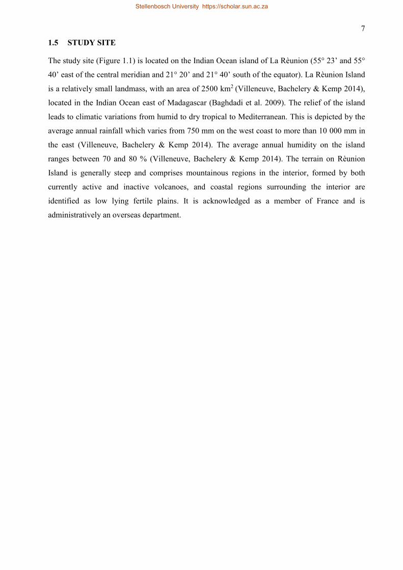
1.5 STUDY SITE

The study site (Figure 1.1) is located on the Indian Ocean island of La Rèunion (55° 23’ and 55°

40’ east of the central meridian and 21° 20’ and 21° 40’ south of the equator). La Rèunion Island

is a relatively small landmass, with an area of 2500 km2 (Villeneuve, Bachelery & Kemp 2014),

located in the Indian Ocean east of Madagascar (Baghdadi et al. 2009). The relief of the island

leads to climatic variations from humid to dry tropical to Mediterranean. This is depicted by the

average annual rainfall which varies from 750 mm on the west coast to more than 10 000 mm in

the east (Villeneuve, Bachelery & Kemp 2014). The average annual humidity on the island

ranges between 70 and 80 % (Villeneuve, Bachelery & Kemp 2014). The terrain on Rèunion

Island is generally steep and comprises mountainous regions in the interior, formed by both

currently active and inactive volcanoes, and coastal regions surrounding the interior are

identified as low lying fertile plains. It is acknowledged as a member of France and is

administratively an overseas department.


8

Figure 1.2 The study site highlighted by the red box on Rèunion Island, located East of Madagascar in the Indian

Ocean.

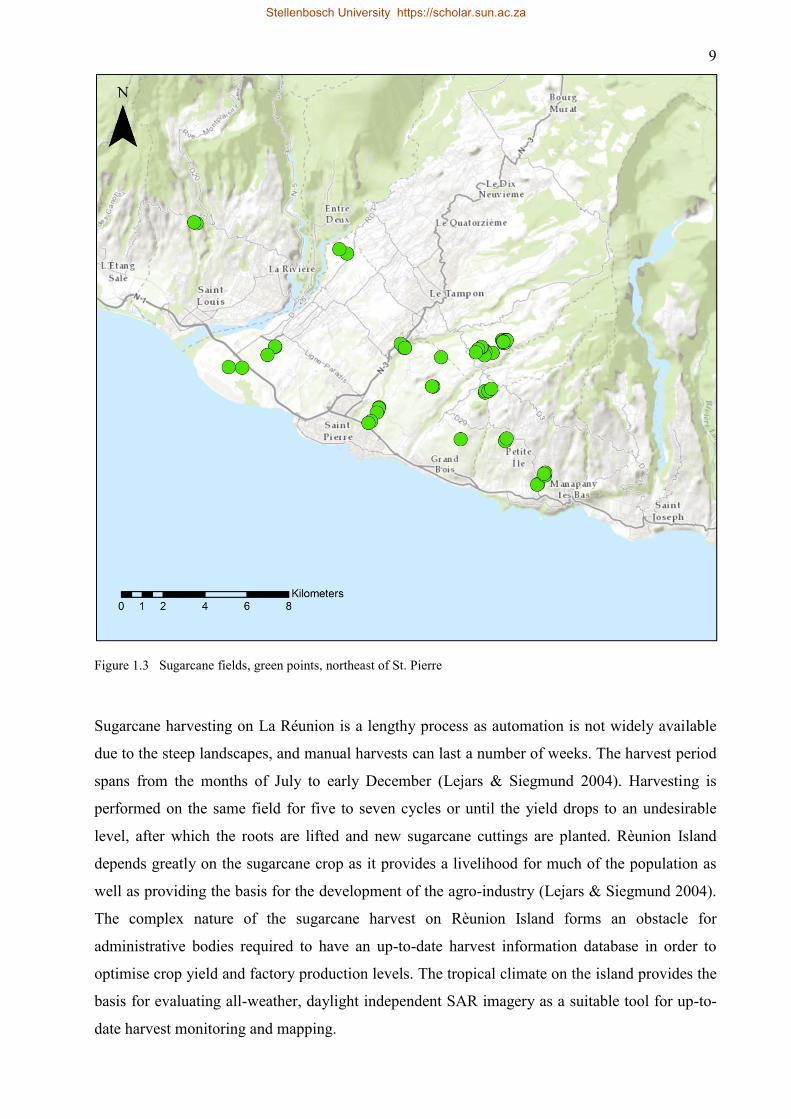
The area under observation, indicated in red (Figure 1.2), comprises approximately 77.22 km2 of

multiple land use zones, which is majorly represented by agricultural parcels, more specifically,

sugarcane. The study investigated sugarcane fields located northeast of the town of Sainte-Pierre

(Figure 1.3), La Rèunion.


9

Figure 1.3 Sugarcane fields, green points, northeast of St. Pierre

Sugarcane harvesting on La Réunion is a lengthy process as automation is not widely available

due to the steep landscapes, and manual harvests can last a number of weeks. The harvest period

spans from the months of July to early December (Lejars & Siegmund 2004). Harvesting is

performed on the same field for five to seven cycles or until the yield drops to an undesirable

level, after which the roots are lifted and new sugarcane cuttings are planted. Rèunion Island

depends greatly on the sugarcane crop as it provides a livelihood for much of the population as

well as providing the basis for the development of the agro-industry (Lejars & Siegmund 2004).

The complex nature of the sugarcane harvest on Rèunion Island forms an obstacle for

administrative bodies required to have an up-to-date harvest information database in order to

optimise crop yield and factory production levels. The tropical climate on the island provides the

basis for evaluating all-weather, daylight independent SAR imagery as a suitable tool for up-to-

date harvest monitoring and mapping.


10

1.6 STRUCTURE OF THESIS

The remainder of the thesis is structured as follows:

Chapter 2 provides an review of the literature relating to RS and more specifically SAR in

sugarcane monitoring, as well as outlining important concepts associated with the data and

methods used in the study. Chapter 3 describes the data acquisition and pre-processing for the

imagery as well as the in situ validation training database. Chapter 3 also outlines the methods

used for Experiment 1 and Experiment 2. Experiment 1 details a method for multi-temporal

single radar feature harvest monitoring. Experiment 2 then introduces a method for single image

classification in order to asses which machine learning classification algorithm proved to be the

most accurate in mapping harvested and unharvested sugarcane fields for both fully-polarimetric

data and a dual polarimetric dataset. Chapter 4 and Chapter 5 presents the results of the above-

mentioned methods and then analytically discusses these results respectively. Concluding the

thesis, Chapter 6 provides conclusions based on the findings, with recommendations for future

studies suggested.


11

CHAPTER 2: LITERATURE REVIEW

The chapter provides a review of the literature relating to remote sensing for land cover

classification and monitoring. Theoretical concepts of SAR are then introduced and agricultural

applications of SAR in literature are discussed.

2.1 REMOTE SENSING FOR LAND COVER CLASSIFICATION AND

AGRICULTURE

Land cover, by definition, is comprised of the physical composition as well as the characteristics

of objects on the Earth’s surface (Cihlar 2000). The location and distribution of land cover plays

a key role in the Earth’s climate and ecological system (Yan, Shakar and El-Ashmawy 2014).

Scientists make use of land cover information as a means to monitor the ever-changing world at

local and global scales. The ability to develop conceptual and predictive models for

understanding Earth’s system processes is greatly advantageous for scientists and authorities

(Dickinson et al. 2013).

The classification of land cover to use as a tool for quantifying and monitoring changes

associated with the Earths’ system processes is identified in scientific communities as a key

element in the study of global change (Henderson-Sellers & Pitman 1992). Land cover maps

have been developed as a product of remote sensing (RS) for several decades (Glanz et al. 2014).

The earth’s surface is displayed as a continuous and consistent representation at a range of

spatial and temporal scales. Satellite imagery has long been viewed as the ideal technology for

the producing land cover classifications of large areas (Gregory 1971; Saint 1980; Iverson, Cook

& Graham 1989). The first global land cover map to be derived as a product of RS was produced

by DeFries and Townshend (1994).

The availability of airborne and spaceborne Earth observation products has greatly increased in

recent years, with further growth predicted in the next decade, allowing land cover information

to be extracted efficiently and in a cost-effective manner (Bayoudh et al. 2015). Further research

into machine learning classification algorithms has contributed to the development of land cover

classification accuracy and the effectiveness of land cover maps (Foody 2002). With the

evolution of these classification algorithms, a new image analysis approach has also developed.

Object-based image analysis (OBIA) has provided a more efficient method for classification

compared to that of pixel-based approaches (Wu & David 2002). The emergence of this concept

has allowed for a link between spatial concepts in multi-scale landscape analysis.


12

Land cover can refer to a large range of land cover types. Agricultural land is considered to be

one of the largest land cover types. Agricultural targets are very dynamic throughout the growing

season, and therefore remote sensing is an attractive approach for agricultural mapping and

monitoring applications. The use of Remote Sensing is ubiquitous in large scale systems for

predicting and monitoring industrial crop harvests and in precision farming services (Todoroff &

Kemp 2016). Acquiring timely information relating to the spatial and structural distribution of

crops as well as optimum conditions for these crops is important for governments at various

levels. With an ever-expanding population, demand on the world’s food resources is increasing.

Productivity of crops is required to be at an all-time high. The use of RS in monitoring

agricultural areas and characterising crop practices provides the basis for management and

optimisation tools (Baghdadi et al. 2009).

This information aids in effective decision-making when aiming to diminish food insecurity risks

(Shi et al. 2014). The large acreages used in modern day agricultural applications have exhausted

the ability of traditional field based surveying techniques to be effective in mapping and

monitoring resources. They are also time-consuming and can become costly, depending on the

observations needed (Engelbrecht, Kemp & Inggs 2013).

RS is an efficient technology for acquiring data to be used for agricultural monitoring. Crop

mapping, specifically, is of high importance for agricultural and economic applications. The

monitoring and surveying of existing crops allow for the production of spaceborne and airborne

earth observation data sources, which play a major role in identifying and discriminating

between different crop types (Mahmoud et al. 2011; Singh et al. 2002), crop distributions and in

predicting future crop yields (Benedetti & Rossini 1991; Lobell et al. 2003).

The use of RS to identify and provide timely information relating to agricultural conditions and

crop growth has improved considerably in the past two decades.

Optical imagery has an extensive history in crop monitoring and surveying. Research conducted

in the 1970s and early 1980s focussed on the use of multispectral images for crop inventory and

production (Moran, Inoue & Barnes 1997). This was demonstrated by Macdonald and Hall

(1980) who investigated the feasibility of using multispectral data for wheat production

estimation. The ever-expanding development of imaging technology and the methods used for

optical image analysis, coupled with the availability of imagery, has created a resourceful

database for agricultural monitoring applications.

Optical imagery makes use of visible and infrared sensors to form images of the earth’s surface

by measuring the solar radiation reflected by ground objects. The wavelengths associated with

visible and infrared regions of the electromagnetic spectrum interact with earth ground objects in


13

such a manner that these objects can be differentiated by their spectral reflectance signatures

(Lillesand, Kiefer & Chipman 2014). The biophysical properties such as plant pigmentation and

internal leaf structure of the agricultural crops under surveillance allow for the development of

these spectral reflectance signatures. This has also led to research related to crop condition

monitoring to be prompted (McNairn et al. 2002). Research aimed at using optical sensors for

the classification and monitoring of crops has been explored extensively (Moran, Inoue &

Barnes 1997; Liu et al. 2010; Vuolo and Atzberger 2012) and continues to do so.

Optical RS has demonstrated itself to be a powerful tool for monitoring of the Earth’ surface on a

global, regional and local scale. This is proven by comprehensive coverage, mapping and

classification of land cover (Simone et al. 2002). Blaes, Vanhalle & Defourney (2005)

investigated the efficiency of crop identification and found when supplementing an optical

dataset with RADAR imagery, that a study was shortened by several months, rather than using

an optical dataset alone with inadequate temporal resolution. The primary limitation associated

with optical imagery is that of incomplete image acquisitions. These are often as a result of poor

weather and atmospheric conditions (Baghdadi et al. 2009). The passive nature of optical

sensors does not allow controlled illumination intensity and geometry as the sensor is dependent

on ambient illumination. Cloud cover is viewed as a source of significant loss of information

and data quality as the wavelengths used for image acquisition do not possess the ability to

penetrate cloud cover, as investigated by Cihlar & Howarth (1994) and Helmer & Ruefenacht

(2005).

The following sections of this chapter will include an overview of the theory relating to SAR as

well as the theory behind image classification and statistical quality control. These sections will

then be followed by an in depth discussion of agricultural applications of SAR.

2.2 SAR INTRODUCTION

SAR is a type of sensor which focusses on mimicking an extended radar antenna in order to

increase spatial resolution of an acquisition. A SAR system works on the principle of measuring

the distance to an object by transmitting an electromagnetic signal (Figure 2.1a), and receiving

an echo containing phase, polarisation and intensity of the backscattered waves, reflected from

the illuminated terrain (Figure 2.1b) (Van Zyl, Arii & Kim 2011) . Unlike optical imaging

sensors, SAR sensors are active sensors. They provide their own source of illumination in the

form of self-propagating microwaves. The use of the microwave region of the electromagnetic

spectrum results in SAR sensors been unaffected by cloud cover. SAR image formation requires

the recording of phase and amplitude information of the microwave echoes received from earth

surface objects (Smith 2002). The SAR makes use of the radar principle to form an image by


14

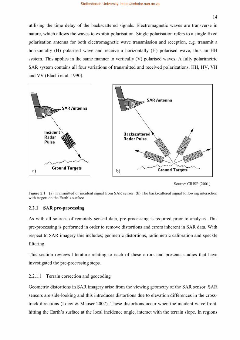
utilising the time delay of the backscattered signals. Electromagnetic waves are transverse in

nature, which allows the waves to exhibit polarisation. Single polarisation refers to a single fixed

polarisation antenna for both electromagnetic wave transmission and reception, e.g. transmit a

horizontally (H) polarised wave and receive a horizontally (H) polarised wave, thus an HH

system. This applies in the same manner to vertically (V) polarised waves. A fully polarimetric

SAR system contains all four variations of transmitted and received polarizations, HH, HV, VH

and VV (Elachi et al. 1990).

Source: CRISP (2001)

Figure 2.1 (a) Transmitted or incident signal from SAR sensor. (b) The backscattered signal following interaction

with targets on the Earth’s surface.

2.2.1 SAR pre-processing

As with all sources of remotely sensed data, pre-processing is required prior to analysis. This

pre-processing is performed in order to remove distortions and errors inherent in SAR data. With

respect to SAR imagery this includes; geometric distortions, radiometric calibration and speckle

filtering.

This section reviews literature relating to each of these errors and presents studies that have

investigated the pre-processing steps.

2.2.1.1 Terrain correction and geocoding

Geometric distortions in SAR imagery arise from the viewing geometry of the SAR sensor. SAR

sensors are side-looking and this introduces distortions due to elevation differences in the cross-

track directions (Loew & Mauser 2007). These distortions occur when the incident wave front,

hitting the Earth’s surface at the local incidence angle, interact with the terrain slope. In regions

a) b)


15

where there are significant terrain disparities the SAR signal experiences distortion of the wave

signal and therefore introduces errors when acquiring an image. These distortions are termed

terrain distortions. Radar foreshortening (Figure 2.2) and layover (Figure 2.3) are two

consequences which result from terrain distortions.

Radar foreshortening is depicted by Figure 2.2. When the emitted radar signal interacts with

steep terrain (e.g. a mountain) and the signal reaches the base of a tall feature before it does the

top, foreshortening will occur.

Source: Natural Resources Canada (2015)

Figure 2.2 Radar foreshortening

This foreshortening is as a result of the radar measuring distance in slant-range. In slant-range

the slope (A to B) will appear to be shortened and the actual length of the slope is incorrectly

represented (A' to B'). The degree to which these measurements are incorrectly represented are

dependent on the angle of incidence in relation to the terrain. Figure 2.2 shows that when the

emitted signal is at a small angle of incidence, the bottom and the top of the slope are

simultaneously imaged (C to D). This results in the actual slope length being represented as zero

in slant-range geometry (C'D').

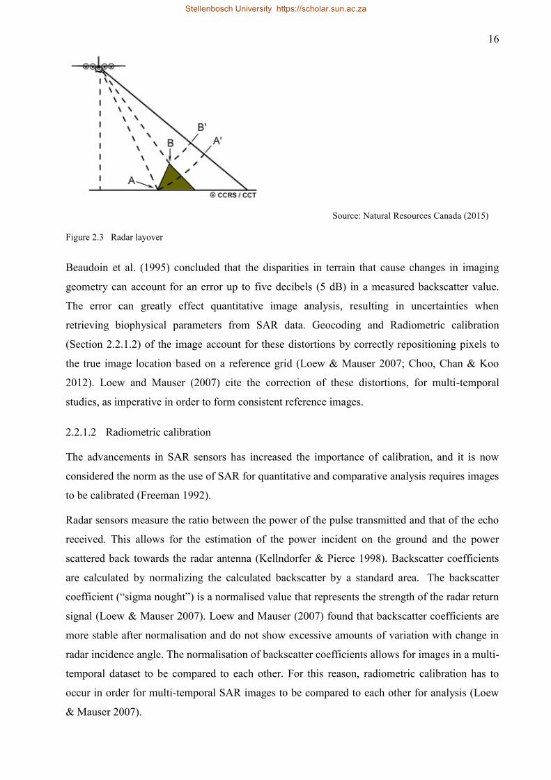
Radar layover (Figure 2.3) has a similar effect to that of foreshortening. It occurs when the top of

a feature (B) is imaged before the emitted signal reaches the bottom of the feature (A). This

results in signal from the top of the feature being returned to the radar before the signal from the

bottom of the feature. For this reason, the top of the feature seems to lean towards the radar and

lays over the bottom of the feature (B' to A'). The degree to which these measurements are

incorrectly represented are dependent on the angle of incidence in relation to the terrain. The

smaller the angle of incidence and the steeper the terrain, the greater the effects (Beaudoin et al.

1995).


16

Source: Natural Resources Canada (2015)

Figure 2.3 Radar layover

Beaudoin et al. (1995) concluded that the disparities in terrain that cause changes in imaging

geometry can account for an error up to five decibels (5 dB) in a measured backscatter value.

The error can greatly effect quantitative image analysis, resulting in uncertainties when

retrieving biophysical parameters from SAR data. Geocoding and Radiometric calibration

(Section 2.2.1.2) of the image account for these distortions by correctly repositioning pixels to

the true image location based on a reference grid (Loew & Mauser 2007; Choo, Chan & Koo

2012). Loew and Mauser (2007) cite the correction of these distortions, for multi-temporal

studies, as imperative in order to form consistent reference images.

2.2.1.2 Radiometric calibration

The advancements in SAR sensors has increased the importance of calibration, and it is now

considered the norm as the use of SAR for quantitative and comparative analysis requires images

to be calibrated (Freeman 1992).

Radar sensors measure the ratio between the power of the pulse transmitted and that of the echo

received. This allows for the estimation of the power incident on the ground and the power

scattered back towards the radar antenna (Kellndorfer & Pierce 1998). Backscatter coefficients

are calculated by normalizing the calculated backscatter by a standard area. The backscatter

coefficient (“sigma nought”) is a normalised value that represents the strength of the radar return

signal (Loew & Mauser 2007). Loew and Mauser (2007) found that backscatter coefficients are

more stable after normalisation and do not show excessive amounts of variation with change in

radar incidence angle. The normalisation of backscatter coefficients allows for images in a multi-

temporal dataset to be compared to each other. For this reason, radiometric calibration has to

occur in order for multi-temporal SAR images to be compared to each other for analysis (Loew

& Mauser 2007).


17

2.2.1.3 SAR filtering

A common anomaly present in coherent imaging systems is speckle noise. This noise is more

prominent in SAR imagery than in optical remotely sensed images. This undesirable effect

causes a pixel-to-pixel variation in intensities and is as a result of random interference between

the coherent returns (McCandless & Jackson 2014). The noise appears as a grainy “salt and

pepper” effect on an image, and is as a result of constructive and destructive interference of the

transmitted signal by different scatterers and degrades both segmentation and classification

accuracy (Lee, Grunes & de Grandi 1999; Lee et al. 2009). When using fully polarimetric data,

filtering is required for accurate interpretation and extraction of polarimetric information (Lee et

al. 2015).

There are two levels of filtering, the first occurs during image formation and is known as multi-

looking, and the second, speckle filtering, is performed post image formation (Gagnon & Jouan

1997). Multi-look filtering averages together several independent images or “looks” of different

portions of the available azimuth spectral bandwidth, or different polarization states of the same

area during image formation (Lillesand et al. 2014). Lee et al. (2008) found that neglecting this

filtering will result in deriving biased and unusable radar parameters, such as entropy, alpha and

anisotropy.

There are two common approaches to speckle reduction following image formation. The most

frequently used approach is accomplished in the spatial domain, where noise is removed by

averaging or statistically manipulating the values of neighbouring pixels (Hervet et al. 1998).

Many spatial filters, which aim to effectively reduce speckle in radar images without eliminating

the fine details, have been devised, namely the Lee Filter (Lee 1980), the Frost Filter and (Frost

et al. 1981) and the popular Lee Sigma Filter (Lee 1983). The Lee Sigma Filter (Lee 1983) does

not require extensive processing resources, however, Lee et al. (2009) found that the filter fails to

retain mean values of pixels, as well as outputting dark unfiltered pixels. Another adaptive

speckle filter, the Boxcar Filter, displays the same properties as the Lee Sigma Filter, in that it

degrades image quality and does not retain polarimetric properties (Lee, Grunes & de Grandi

1999).

A spatial filter proposed by Lee, Grunes & de Grandi (1999), known as the Refined Lee Filter,

improved on the previously mentioned Lee Filter by identifying cells that contain noise and

using a neighbourhood of eight cells to assign a filtered value to this cell. In doing so a more

accurate filtering method is applied. This filter effectively preserves polarimetric information and

subtle details (Qi et al. 2012).


18

As stated in literature, it is important to apply a polarimetric speckle filter prior to analysis in

order to achieve reliable results. This is outlined by Ban and Wu (2005) who performed a study

using SAR C-band to compare filtered and unfiltered images for land cover classification. They

found that overall accuracies improved by over 40% just by spatially filtering the images. Very

little investigation has been done into comparing the levels of accuracy each filter is able to

achieve, as well as investigating various parameters within the filters, such as window size and

number of looks.

2.2.2 SAR backscatter

A SAR system records the echo received from a transmitted electromagnetic signal. The received

echo is in the form of intensity per pixel. The intensity values are converted to a physical

quantity known as the backscattering coefficient. Backscatter coefficients are calculated by

normalizing the calculated backscatter by a standard area (Loew & Mauser 2007). The

backscattering coefficient, also known as the normalised radar cross-section, is measured in

decibel (dB) units and is calculated using the radar equation.

2.2.2.1 Factors affecting SAR backscatter

Baghdadi et al. (2008) state that the nature of the received microwave signal, or backscatter, is a

function of the combination of radar parameters and properties of the earth surface objects. The

radar parameters include frequency, polarization and incidence angle. Backscatter for a target on

the earth’s surface at a particular wavelength will vary depending on topography, the size of the

scatterers and the dielectric properties which relate to moisture content.

Frequency - The frequency of a SAR system defines the wavelength at which the system

operates. The microwave region of the electromagnetic spectrum is divided into bands and these

are used for acquisition of SAR data. The most common bands used for commercial applications

and research are L-, C- and X-bands. In general microwaves are sensitive to features which are

of similar size to that of the wavelength, while smaller objects appear transparent (Rosenqvist et

al. 2007). The applications of SAR are dependent on the frequency. The longer wavelength, L-

band, has a relatively high penetration depth into vegetation and soil compared to that C- and of

X-band sensors (Suga & Konishi 2008; Inoue & Sakaiya 2013). These penetrative abilities are

shown to be inappropriate for estimating crop biomass as displayed by Baghdadi et al. (2009),

who showed that C-band is better for determining differences in crop type between low biomass

crops.

C-band with polarimetric capabilities can estimate the phenological stage without any

supplemental information (Lopez-Sanchez et al 2014). C-band data has also shown the ability to


19

differentiate between different crop types (Baghdadi et al 2009). Other studies have assessed the

capability of C-band backscatter to assess biophysical variables in paddy rice, revealing that C-

band backscatter is highly affected by the leaf structure of the plant and for this reason can be

compared to Normalized Difference Vegetation Indices derived from optical data (Inoue,

Sakaiya & Wang 2014). These studies indicate the importance of selecting the appropriate SAR

sensor and wavelength for a specific application.

Incidence angle – The incidence angle at which the sensor illuminates the target object is an

important configuration of the SAR sensor especially for the effective monitoring of agriculture.

Steeper incidence angles have proven to display higher backscatter intensities, while shallower

incidence angles show more interaction with vegetation and less influence from soil roughness

and moisture (Moran et al. 1998).

McNairn and Brisco (2004) conducted a study to assess the performance of C-band polarimetric

SAR for an agricultural application. Conclusions relating to incidence angle revealed that at a

steep incidence angle, backscatter intensities are higher, and horizontally polarised waves

penetrate the vegetation canopy to a greater extent than vertically polarized waves. Cable et al.

(2014) support this by stating that the varying incidence angles cause large differences in

responses found in the VV and HH bands and found there to be an inverse relationship between

incidence angle and backscatter intensity.

O'Grady, Leblanc and Gillieson (2011) assessed the relationship of C-band radar backscatter

with the angle of incidence. They concluded that a change in incidence angle results in a change

in backscatter intensity, this change is based on the structural and dielectric properties of the

target object, thereby indicating that the incidence angle is an important factor to consider when

deciding on imagery to use for operational and commercial use.

Polarisation - Electromagnetic waves are transverse in nature, which allows the waves to exhibit

polarisation. Single polarisation refers to a single fixed polarisation antenna for both

electromagnetic wave transmission and reception, e.g. transmit a horizontally (H) polarised wave

and receive a horizontally (H) polarised wave, thus an HH system.

Extending on this, a fully polarimetric SAR system contains all four variations of transmitted and

received polarizations, HH, HV, VH and VV. Polarimetric radar data can provide much more

detailed information about the surface geometry, terrain cover, and subsurface discontinuities

than backscatter intensity alone (Elachi et al. 1990). Each of these polarisations is sensitive to the

characteristics and properties associated with the earth’s surface objects, posing PolSAR as a

powerful tool for the identification and extraction of earth surface objects (Kourgli et al. 2010).


20

Lopez-Sanchez, Cloude and Ballester-Berman (2014) investigated the polarimetric response of

rice fields and, using these, were able to develop a classification system which achieved a 96%

accuracy in retrieving crop phenology. In this identifying fully polarimetric SAR as a tool for

agricultural monitoring as it has the ability to yield information about the dielectric properties,

shape and orientation of the plant.

The different polarisations and combinations thereof each have their own benefits when using

fully polarimetric SAR data. Vertically orientated waves (VV) show large amounts of interaction

with vertical structures such as stems. The cross-polarisation (HV and VH) channels have

however shown to be more effective in agricultural mapping (Baghdadi et al. 2009). This is as a

result of broadleaf vegetation causing multiple-bounce scattering, resulting in some complete

depolarisation of the wave (Srivastava et al. 2009). Consequently, to obtain more accurate crop

maps or to monitor crop productivity, preference should be given to HV-polarised images.

Dual polarimetric SAR systems generally exclude one of the transmitted polarisations. Hereby

excluding either an H or V polarisation when transmitting a signal. These systems do however

receive both H and V backscattered polarizations, therefore recording half of the full scattering

matrix, either HH-HV or VV-VH, if the transmitting polarisation remains the same (Ainsworth,

Kelly & Lee 2009).

With the advancement in SAR technology the spatial resolutions of the sensors are becoming

finer and the conventional single-polarization mode is moving towards dual or full polarimetric

modes. Comparison studies have been conducted between fully polarimetric datasets and dual

polarimetric datasets, in order to understand the additional information presented by fully

polarimetric datasets (Ainsworth, Kelly & Lee 2009; Furtado, Silva & Nova 2016). Findings

from these studies reveal that in both cases the fully polarimetric datasets performed better in

image classification.

2.2.3 SAR data structure

The main data formats for describing the fully polarimetric signal are the scattering matrix, the

covariance matrix and the coherency matrix.

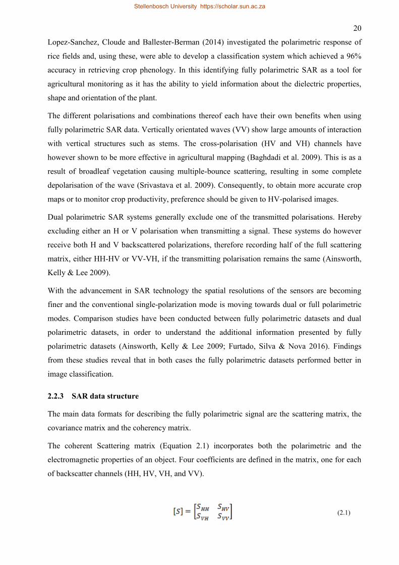
The coherent Scattering matrix (Equation 2.1) incorporates both the polarimetric and the

electromagnetic properties of an object. Four coefficients are defined in the matrix, one for each

of backscatter channels (HH, HV, VH, and VV).

(2.1)


21

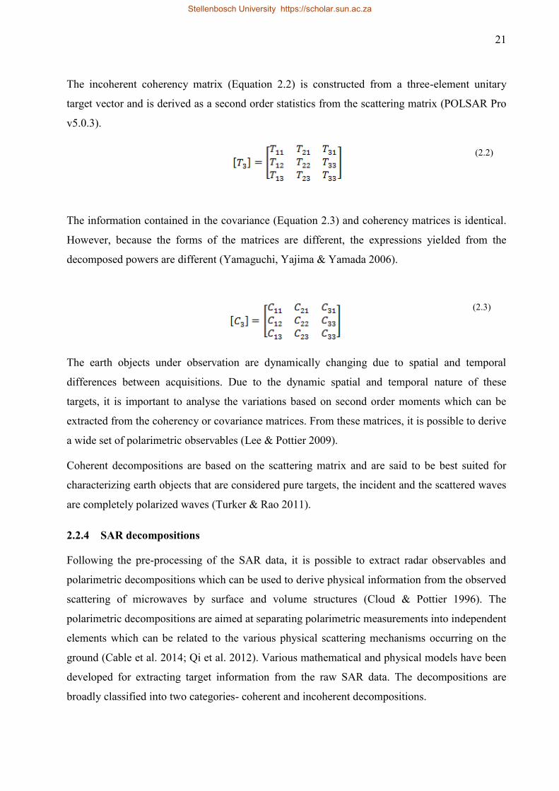
The incoherent coherency matrix (Equation 2.2) is constructed from a three-element unitary

target vector and is derived as a second order statistics from the scattering matrix (POLSAR Pro

v5.0.3).

(2.2)

The information contained in the covariance (Equation 2.3) and coherency matrices is identical.

However, because the forms of the matrices are different, the expressions yielded from the

decomposed powers are different (Yamaguchi, Yajima & Yamada 2006).

(2.3)

The earth objects under observation are dynamically changing due to spatial and temporal

differences between acquisitions. Due to the dynamic spatial and temporal nature of these

targets, it is important to analyse the variations based on second order moments which can be

extracted from the coherency or covariance matrices. From these matrices, it is possible to derive

a wide set of polarimetric observables (Lee & Pottier 2009).

Coherent decompositions are based on the scattering matrix and are said to be best suited for

characterizing earth objects that are considered pure targets, the incident and the scattered waves

are completely polarized waves (Turker & Rao 2011).

2.2.4 SAR decompositions

Following the pre-processing of the SAR data, it is possible to extract radar observables and

polarimetric decompositions which can be used to derive physical information from the observed

scattering of microwaves by surface and volume structures (Cloud & Pottier 1996). The

polarimetric decompositions are aimed at separating polarimetric measurements into independent

elements which can be related to the various physical scattering mechanisms occurring on the

ground (Cable et al. 2014; Qi et al. 2012). Various mathematical and physical models have been

developed for extracting target information from the raw SAR data. The decompositions are

broadly classified into two categories- coherent and incoherent decompositions.


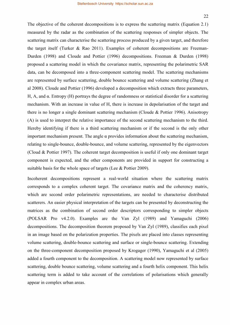
22

The objective of the coherent decompositions is to express the scattering matrix (Equation 2.1)

measured by the radar as the combination of the scattering responses of simpler objects. The

scattering matrix can characterise the scattering process produced by a given target, and therefore

the target itself (Turker & Rao 2011). Examples of coherent decompositions are Freeman-

Durden (1998) and Cloude and Pottier (1996) decompositions. Freeman & Durden (1998)

proposed a scattering model in which the covariance matrix, representing the polarimetric SAR

data, can be decomposed into a three-component scattering model. The scattering mechanisms

are represented by surface scattering, double bounce scattering and volume scattering (Zhang et

al 2008). Cloude and Pottier (1996) developed a decomposition which extracts three parameters,

H, A, and α. Entropy (H) portrays the degree of randomness or statistical disorder for a scattering

mechanism. With an increase in value of H, there is increase in depolarisation of the target and

there is no longer a single dominant scattering mechanism (Cloude & Pottier 1996). Anisotropy

(A) is used to interpret the relative importance of the second scattering mechanism to the third.

Hereby identifying if there is a third scattering mechanism or if the second is the only other

important mechanism present. The angle α provides information about the scattering mechanism,

relating to single-bounce, double-bounce, and volume scattering, represented by the eigenvectors

(Cloud & Pottier 1997). The coherent target decomposition is useful if only one dominant target

component is expected, and the other components are provided in support for constructing a

suitable basis for the whole space of targets (Lee & Pottier 2009).

Incoherent decompositions represent a real-world situation where the scattering matrix

corresponds to a complex coherent target. The covariance matrix and the coherency matrix,

which are second order polarimetric representations, are needed to characterise distributed

scatterers. An easier physical interpretation of the targets can be presented by deconstructing the

matrices as the combination of second order descriptors corresponding to simpler objects

(POLSAR Pro v4.2.0). Examples are the Van Zyl (1989) and Yamaguchi (2006)

decompositions. The decomposition theorem proposed by Van Zyl (1989), classifies each pixel

in an image based on the polarization properties. The pixels are placed into classes representing

volume scattering, double-bounce scattering and surface or single-bounce scattering. Extending

on the three-component decomposition proposed by Krogager (1990), Yamaguchi et al (2005)

added a fourth component to the decomposition. A scattering model now represented by surface

scattering, double bounce scattering, volume scattering and a fourth helix component. This helix

scattering term is added to take account of the correlations of polarisations which generally

appear in complex urban areas.


23

Alberga, Satalino & Staykova (2008) performed a study of land cover classification in order to

make inferences about the ability of coherent and incoherent decompositions for classification.

Their results revealed that the Freeman Durden decomposition shows great ability in land cover

classification, however, a limited dataset was used and they could place no validity on the

results. This was further supported by Turkar and Rao (2011) when comparing classifications

based on different decompositions. They concluded that the Van Zyl decomposition was able to

produce superior classification accuracy to the other decompositions, however when all the

features across all decompositions were used for classification, volume scattering from the Van

Zyl and Freeman-Durden decompositions contributed the most to the overall accuracy.

2.3 IMAGE CLASSIFICATION USING SAR

Image classification is the process of grouping all pixels or objects of similar spectral and spatial

information into categories. These categories are, as in the case of this study, generally real-

world objects. Image classification makes use of pre-processed imagery. Using the pre-processed

imagery, a pixel or object-based classification approach can be selected. The classification

approach selected may require segmentation of the image followed by feature selection or

dimensionality reduction. It is then required to selected the appropriate classifier for the dataset

and project requirements.

2.3.1 Object vs pixel based classifications

Traditionally, pixel-based classifications were employed for land cover classification. However,

these classification techniques have shortcomings when high resolution imagery is used. In

pixel-based classification, each individual pixel is classified as a particular land cover type. An

increase in spatial resolution results in an increase in sub-class elements. The increase in these

sub-class elements leads to great spectral variability within classes, creating confusion when

aiming to separate spectrally mixed land cover types (Wang, Sousa & Gong 2004). With the

recent advancements in sensor development and improvement in spatial resolution, there has

been a shift in methods used for classification. The evolution of these classification algorithms,

has led to a new image analysis approach being developed. An alternative solution, object-based

image (OBIA) classification, makes use of incorporating information on the spatial

neighbourhood properties into the classification process (Shaban & Dikshit 2001). Object-based

image analysis has provided a more efficient method for classification compared to that of pixel-

based approaches. The emergence of this concept has allowed for a link between spatial concepts

in multi-scale landscape analysis (Wu & David, 2002).


24

The efficiency of an object-based method was demonstrated by Myint et al. (2011), who

investigated how pixel-based approaches perform compared to object-based approaches when

classifying urban land cover. The spectral information alone, using the pixel-based approach,

was able to reach an overall accuracy of 63.33%. The object-based approach proved far superior

in the classification of urban land cover producing an overall accuracy of 90.40%. The

superiority of object-based image classification techniques was further demonstrated in an

agricultural context by Duro, Franklin and Dube (2012). They made use of selected machine

learning algorithms to classify agricultural landscapes. Findings from the study indicate a

significant difference in classification accuracy between the two approaches. When using the

SVM classifier, the accuracy of the object-based method (95%) improved on that of the pixel-

based method (89%) by 6%.

There has been extensive research to show the superiority of object-based image classification,

however there are shortcomings when using the technique and these are identified by Myburgh

and Van Niekerk (2014). The conclusion drawn from their results indicate that object-based

classification techniques introduce large data dimensionality which results from the added

features that can be derived when using object-based image analysis. This will result in increased

processing time and can potentially lower classification accuracy (Myburgh & Van Niekerk

2014).

Based on the results presented by the above-analysed literature, this study makes use of an

object-based image classification approach. The large data dimensionality associated with this

approach requires that feature reduction techniques be employed prior to classification.

2.3.2 Feature selection

The large amount of features which can be created when using object-based image classification

introduces a high data dimensionality (Rodriguez-Galiano et al. 2011). This high data

dimensionality is as a result of elements, or features, that can be derived from objects. The

elements associated with SAR data can be derived from the backscatter bands as well as the

polarimetric decompositions (Chen, Chen & Lee 2003).

The large dimensionalities associated with the data pose challenge for users, as many

classification algorithms have difficulty in dealing with the large number of input features (Duro,

Franklin & Dube 2012). The use too many features can also lead to the “curse of

dimensionality”, where classifiers are over-trained, resulting in poor classification accuracies and

poor models that are not representative of the real world. The effective use of classification

algorithms requires a subset of the data to be used. Feature selection or reduction has become an


25

indispensable component of the machine learning process (Kumar & Minz 2014). Feature

selection removes redundant and irrelevant features from the feature dataset, with the aim of

improving classification accuracy and reducing computational requirements.

In remote sensing, feature reduction methods can form part of two broad categories. The first

includes feature reduction methods known as wrappers. These methods are embedded within the

classifier, meaning that the features selected are only suitable for classification performed by the

classifier itself. Two examples of this are; Classification and Regression Trees (CART) (Chubey,

Franklin & Wulder 2006; Laliberte et al. 2012; Yu et al. 2006) and Random Forests (RF)

(Rodriguez-Galiano et al. 2011), which have both been applied extensively in feature reduction

for object-based image classification. The feature reduction technique used in this study is,

however, of a filter nature. This means the methods used produce subset of the data that can be

used for image classification across all classifiers. These methods include Exploratory Factor

Analysis (EFA) and Analysis of Variance (ANOVA).

EFA is used by researchers who are uncertain of how variables will operate. EFA aims to

describe the variability among observed variables in terms of a reduced number of unobserved

variables know as factors. Linear combinations of these factors are used to model the observed

variable, thereby estimating how much of the variability in the data was as a result of the

common factors (Matsunaga 2010). ANOVA is used to determine whether there are any

significant differences between the means of two or more independent groups (Kayzoglu &

Mather 2002).

This study made use of a combination of the latter two feature reduction methods, in a multi-

tiered featured selection technique that has not been applied in the realm of remote sensing as yet

and for this reason literature relating to the topic is scarce.

2.3.3 Classification algorithms

After feature reduction, a subset of the original dataset remains for use in image classification.

The purpose of the classification process is to group all pixels or objects of similar spectral and

spatial information into categories. These categories are representative of land cover classes or

themes on the ground. Classification is used in order to produce thematic maps of these land

cover classes and display them with a unique label (Lillesand & Kiefer 2014). When classifying,

there are two main techniques that can be considered for use: unsupervised classification and

supervised classification (Lee, Grunes & De Grandi 1999). Unsupervised classification is based

on grouping pixels with similar properties. There is little interaction with a user and the user will

only enter the number of classes to be generated. With this information, the algorithm generates


26

clusters. Unsupervised methods are not processing intensive. A major disadvantage is that the

spectral classes do not always correspond to informational classes. Another disadvantage is that

spectral classes tend to change over time and thus class information is not transferable (Lee,

Grunes & Pottier 2001). Literature identifies supervised machine learning algorithms as

becoming more popular to use for image classification as they are able to handle large amounts

of complex data for training and classification (Rodriguez-Galiano et al. 2012). Further research

into machine learning classification algorithms has greatly contributed to the development of

land cover classification accuracy and the effectiveness of land cover maps (Foody, 2002).

The increased application and results achieved using supervised machine learning algorithms has

led to supervised classification being used in this study, however Shang et al. (2009) indicates

that when choosing a classifier, it is important to consider data requirements, availability of

training data, and computation requirements associated with the classifier.

Supervised machine learning classifiers are discussed widely in literature. Five common

supervised classifiers were identified and are discussed below.

Nearest Neighbour (NN) - When using the Nearest Neighbour classifier, a pixel or object is

classified by calculating the distance to the nearest training case. The class assigned to the

training case is then assigned the object or pixel. K-Nearest Neighbour (KNN) extends on this by

taking the K nearest points and assigning the class based on the majority of points (Fix and

Hodges 1951). The KNN classifier requires the tuning of only one free parameter and the

classifier is not parametric. Therefore, no statistical distribution of the data is assumed (Cover &

Hart 1967). Melgani and Bruzzone (2004) compared supervised classification accuracy using

hyperspectral imagery. The results show that the KNN classifier was able to successfully classify

the data with an overall accuracy of 83.94%, though KNN was outperformed by SVM in this

study. The KNN is not commonly applied in literature as the more advanced classifiers often

outperform the simple KNN classifier.

Maximum Likelihood (ML) - The Maximum Likelihood classifier is commonly used for

classification of remotely sensed images. It is a parametric classifier, which calculates the mean,

variance and covariance of the training data and uses it to form a distribution of each class

(Albert 2002). Otukei, Blascke and Collins (2014) made use of the ML classifier in order to

assess the potential of TerraSAR-X and ALOS PALSAR data for land cover mapping. The

classifier achieved an accuracy of 43.9% and 86% for the TerraSAR-X and ALOS PALSAR data

respectively. The poor performance of the classifier for the TerraSAR-X data, is in line with Ma

et al. (2013) who do not recommend using the ML classifier for SAR imagery. Another


27

disadvantage of this classifier, as found by Myburgh and van Niekerk (2014), is that it is unable

to perform under high dimensionality conditions.

Support Vector Machines (SVM) - Support Vector Machines classifiers were developed as a

binary classifier, based on statistical learning theory and structural risk minimisation (Vapnik

1995). The classifier aims to separate two or more classes with the use of an optimal separating

hyperplane. The separation of multiple classes is automated through the implementation of a

kernel function (Mountrakis, Im & Ogole 2011). SVM’s have recently been implemented for

image classification in remote sensing due to their superior classification accuracies and ability

to handle large data input (Melgani & Bruzzone 2004; Foody, 2002). In addition to the

advantages mentioned, SVM’s have been found to produce higher classification accuracies when

compared to other classifiers such as ML and Artificial Neural Networks (Melgani & Bruzzone

2004; Mountrakis, Im & Ogole 2011). The superior accuracy levels and other mentioned

advantages are demonstrated by Rumpf et al. (2010) in an agricultural context. They aimed to

develop an automated method, using nine spectral vegetation indices, for plant disease detection

using hyperspectral reflectance data. The SVM classifier was able to discriminate between

healthy and diseased leaves with an accuracy of 97% and multiple classifications between

healthy leaves and leaves with symptoms of three separate diseases achieved an accuracy of

86%. Despite superior classification accuracy, SVM can be poses a disadvantage with extended

processing times (Chan, Laporte & Defries 2003).

Decision Trees (DT) - Decision Trees for identification and classification of objects was first

reported by Hunt, Marin and Stone (1996). Since then DT classifiers have shown great potential

for land cover classification using remotely sensed data (Friedl & Brodley 1997; Sharma, Gosh

& Joshi 2013; Chasmer et al. 2014). Essentially a DT classifier evaluates a set of variables,

identifies which of these variables are most important and then produces a set of trees which best

separate the data into the respective classes (Quinlan 1987). DT classifiers are high variance

classifiers, meaning that they are sensitive to the precise spatial distribution of samples and if

training data is limited, the classifier can fit to noise (Chasmer et al. 2014). DT classifiers are,

however, easy to run, they show fast prediction capabilities, perform variable selection implicitly

and have shown to achieve high levels of accuracy when used for classifying imagery (Friedl &

Brodley 1997; Lillesand, Kiefer & Chipman 2014).

Friedl and Brodley (1997) reported that DT classifiers were superior in classification of land

cover when compared to both maximum likelihood and linear discriminant function classifiers.

This was supported in literature by Sharma, Gosh and Joshi (2013) who, when using DT, ML

and an unsupervised ISODATA clustering method to classify land cover types within the zone of


28

discontinuous permafrost, found that the DT classifier (90%) far outperformed both the ML

(76.67%) and ISODATA (57.5%) classifiers.

Random Trees (RT) - One of the most recent classification algorithms proposed is the Random

Trees classifier (Ho 1995). The RT classifier makes use of the same method as decision trees,

but uses the best split of input features at every division of the decision tree (Rodriguez-Galiano

et al. 2011). The classifier then iteratively creates decisions trees using the best split (Rodriguez-

Galiano et al. 2011). This growth of the decision trees allows for the classifier to select the most

popular class for a selected split (Pal 2005). This has proved to produce significant increases in

land cover classification accuracy (Breiman 2001; Pal 2005; Rodriguez-Galiano et al. 2012).

Pal (2005) compared the land cover classification accuracies achieved by a RT, with that

achieved by a SVM method. His results indicate that the RT classifier was able to perform

equally as well as the SVM’s. He also cited that the RT classifier requires less user defined

parameters, can handle categorical data and data with missing values. The implicit feature

selection performed by RT classifiers, provides a feature importance index which can be used for

further feature selection (Waske & Braun 2009). The application of RT’s to SAR data was

investigated by Du et al. (2015), who made use of SVM’s, RT and a variation of RT, Rotation

Forest. The study concluded that the RT classifier outperformed the SVM classifier achieving an

overall accuracy of 83.8%. While the Rotation Forests improved on this accuracy the RT

classifier was time and computationally efficient and was therefore cited as superior.

The use of these classification algorithms for agricultural classification using SAR imagery is

discussed in Section 2.5.4. The following section introduces Shewhart individual control charts

and review literature on these charts.

2.4 SHEWHART INDIVIDUAL CONTROL CHARTS

The use of control charts as a tool for monitoring the quality of a process, is regarded as a

powerful monitoring tool due to the statistical nature of the monitoring. Applying a statistical

control procedure is an important factor in a system of quality control. One of these procedures

which is widely used and recognised is the Shewhart individual control charts.

Traditionally, the method, proposed by Walter Shewhart in the 1920s, was used in controlling

the variance in manufacturing processes and became known as the Shewhart individual control

chart (Shewhart 1931). The use of the chart in manufacturing processes aims to minimise costs

associated with inspections and rejections, which aids in maintaining quality at a satisfactory and

cost-reduced standard (Hotelling 1932). The chart is based on the moving range (MR) of a

process. The moving range is described as the difference or ratio from one measurement to the


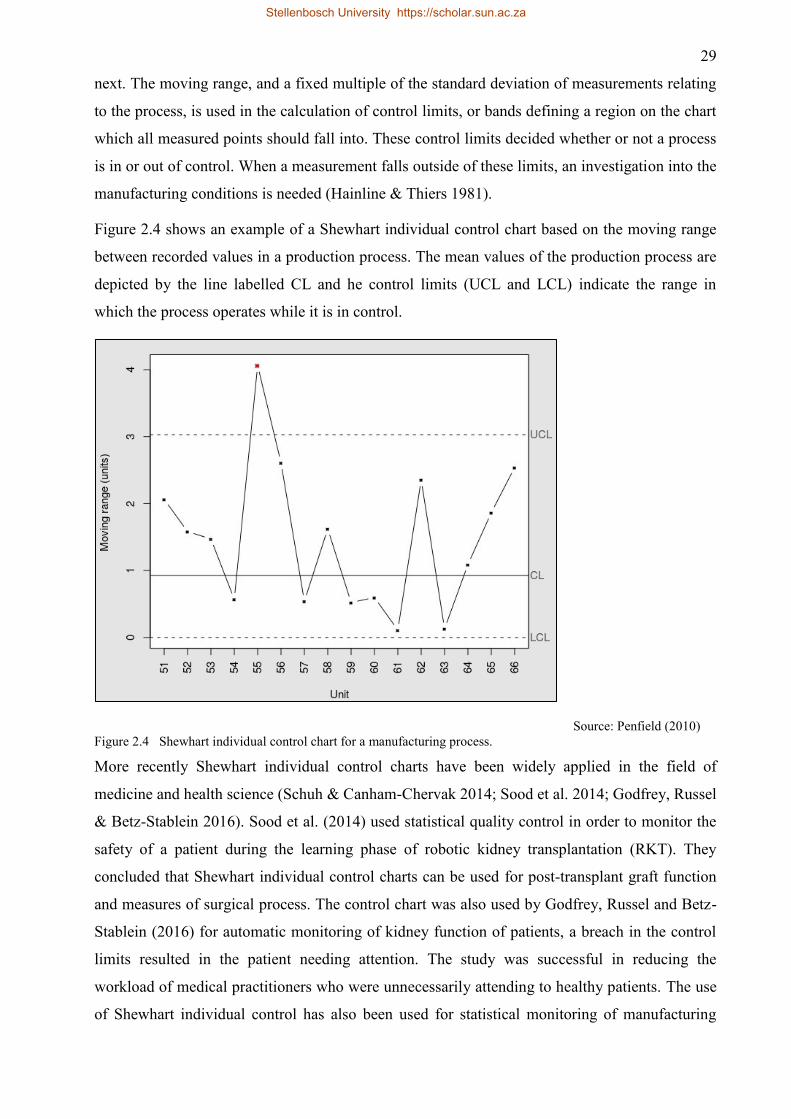
29

next. The moving range, and a fixed multiple of the standard deviation of measurements relating

to the process, is used in the calculation of control limits, or bands defining a region on the chart

which all measured points should fall into. These control limits decided whether or not a process

is in or out of control. When a measurement falls outside of these limits, an investigation into the

manufacturing conditions is needed (Hainline & Thiers 1981).

Figure 2.4 shows an example of a Shewhart individual control chart based on the moving range

between recorded values in a production process. The mean values of the production process are

depicted by the line labelled CL and he control limits (UCL and LCL) indicate the range in

which the process operates while it is in control.

Source: Penfield (2010)

Figure 2.4 Shewhart individual control chart for a manufacturing process.

More recently Shewhart individual control charts have been widely applied in the field of

medicine and health science (Schuh & Canham-Chervak 2014; Sood et al. 2014; Godfrey, Russel

& Betz-Stablein 2016). Sood et al. (2014) used statistical quality control in order to monitor the

safety of a patient during the learning phase of robotic kidney transplantation (RKT). They

concluded that Shewhart individual control charts can be used for post-transplant graft function

and measures of surgical process. The control chart was also used by Godfrey, Russel and Betz-

Stablein (2016) for automatic monitoring of kidney function of patients, a breach in the control

limits resulted in the patient needing attention. The study was successful in reducing the

workload of medical practitioners who were unnecessarily attending to healthy patients. The use

of Shewhart individual control has also been used for statistical monitoring of manufacturing


30

processes (Aliverdi, Naeni & Salehipour 2013; Biswas, Masud & Kabir 2015). Biswas, Masud

and Kabir (2015) collected data for six months within a weaving mill, the data related to four

characteristics associated with thread bales. They used measurements of each of these four

characteristics in order to construct standards, or ideals, for the quality of each thread bale. The

results achieved aided in improving the quality of the thread bales produced by the weaving mill.

The use of Shewhart individual control charts have been widely applied for statistical monitoring

of a process. However, the chart has not been used in the realm of remote sensing and therefore

has been identified to be used in this study for sugarcane harvest monitoring using SAR. The

chart serves the purpose of monitoring a process and identifies any anomalies in the process. The

anomaly in the case of this study will be a harvested crop.

2.5 SYNTHETIC APERTURE RADAR APPLICATIONS IN AGRICULTURE

With the advancements in SAR instruments in recent years, the data and products produced from

it relating to SAR, is expanding at a rapid rate. This expansion, coupled with the ability of the

radar sensors to acquire imagery independent of weather and daylight, has resulted in SAR data

being used in a variety of applications. SAR, with the development of interferometry, has been

widely applied in geological fields to produce maps showing surface deformation or elevation

(Monserrat, Crosetto & Luzi 2014). Another field where SAR is deemed as a suitable tool for

analysis is forestry as the microwave wavelengths associated with SAR allow for penetration of

forest vegetation (Thapa et al. 2013; Minh et al. 2014; Kellndorfer et al. 2014). Urban

monitoring applications using SAR (Scmitt & Stilla 2014) have been widely employed with the

development of polarimetric decompositions. Another important application of SAR has been in

the field of oceanography. One of the most important applications of SAR has been in the

military. Potential military applications include detection and recognition of military vehicles

beneath a canopy, detection and recognition of complex urban structures, detection of tall

obstructions that could prove hazardous to low flying air vehicles, and detection and recognition

of moving targets (El-Darymli et al. 2013).

This study focuses on the use of SAR for agriculture. A review of the literature relating to SAR

and agriculture is provided in section 2.5.1.

2.5.1 General SAR in agriculture

The use of Synthetic Aperture Radar (SAR) data for land cover information extraction, more

specifically for agriculture, was implemented at a far later stage than optical RS data (Mahmoud

et al. 2011). Using SAR data for agricultural monitoring applications provides an advantage over

optical imagery in that SAR possesses the ability to acquire imagery with large spatial and


31

temporal variability regardless of atmospheric conditions (McNairn et al. 2002) and is thus able

to produce complete consistent datasets. This comes as a result of the penetrative abilities of the

wavelength related to the microwave region of the electromagnetic spectrum. The vector nature,

comprised of phase and amplitude, of these electromagnetic waves can also be taken into

account as they provide scattering information for discerning and identifying Earth objects

(Alberga 2007). The nature of agriculture requires images to be acquired frequently enough in

order to monitor important crop growth stages (Karjalainen, Kaartinen & Hyyppä 2008).

Suga & Konishi (2008) demonstrated the effect of using different frequencies with the use of a

multi-frequency rice crop monitoring study. They concluded that L-band data penetrated further

into the rice plant as opposed to shorter wavelengths (X-band) which interacted with the grain

water content of the plant. This was further supported by Inoue and Sakaiya (2013) who

concluded that, due to X-band interaction with the rice grain rather than the actual plant

structure, X-band data can be used to determine the assessment of rice grain yield. Koppe et al.

(2013) made use of multi-temporal TerraSAR-X data for the monitoring of rice crops in Sanjiang

Plain in Northeast China. Their results show that there is a strong correlation between the VV

polarimetric channel and the plant stem early in the plant growth stage; however, this correlation

reduces as the leaf structure of the plant develops. They concluded that X-band data is useful in

the monitoring of biomass during the early growing season; however, due to an early saturation

level compared to longer wavelengths, it is not useful in the later growth stages of the rice plant.

The conclusions made by Koppe et al. (2013) do not concur with those made by Inoue and

Sakaiya (2013). Baghdadi et al. (2008) found that the shorter X-band wavelengths can be used

to discern between ploughed and unploughed fields. This is due to X-band being affected by the

surface roughness based on its inability to penetrate the surface.

The potential of SAR in monitoring soil and vegetation parameters has been investigated by

several other authors (Wegmuller & Werner 1997; Le Hegarat-Mascle et al. 2002). These studies

reveal that microwave backscattering is sensitive to vegetation biomass (Dobson, Pierce and

Ulaby 1996). The scattering, attenuation, and emission of electromagnetic energy vary with crop

type and development stage as the magnitude of backscatter received by the radar system is

determined by the dielectric property of a target. Thus, SAR can be used to detect contrast

among vegetation with varying dielectric properties.

The microwave signals’ sensitivity to soil and vegetation parameters vary depending on the

wavelength used by the sensor (Dobson, Pierce and Ulaby 1996). The shorter of the wavelengths

used in SAR, X-band and C-band, tends to interact predominantly with the top sections of

agricultural canopies as they display sensitivity to leaves and small branches. L-band and P-


32

band data, due to a longer wavelength, possess penetrative abilities. They are therefore able to

penetrate the vegetation canopies and interact with the stem of plants and the soil (Baghdadi et

al. 2008). Supporting this Dobson, Pierce and Ulaby (1986) have demonstrated that it is simpler

to use L-band data to differentiate soil roughness classes than using X-band or C-band data in

agriculture.

Research into using a fully polarimetric C-band frequency sensor to estimate phenological stage

of rice fields was conducted by Lopez-Sanchez et al. (2014). Using a simple classifier, an

accuracy of 96% was achieved, correctly validating 44 out of 46 land parcels. C-band with

polarimetric capabilities can estimate the phenological stage without any supplemental

information. Lopez-Sanchez et al. (2014) concluded that L-band data should be merged with C-

band data as it possesses better ability to discriminate crop phenology in the advanced crop

growth stage.

In a review of the use of SAR for agricultural monitoring applications, Karjalainen, Kaartinen

and Hyyppä (2008) devised a classification of SAR use in agricultural monitoring. The

categories where SAR has been identified as an effective tool within the agricultural domain

include:

1. Mapping of yield losses;

2. Estimation or prediction of crop yield;

3. Assessment of the area under cultivation;

4. Crop species interpretation;

5. Precision farming, where maximum yield is sought with minimum fertilization; and

6. Control of agricultural subsidies.

2.5.2 SAR in harvest monitoring

The use of SAR for harvest monitoring has not been extensively investigated. The studies

conducted focus on crop monitoring rather than crop harvest monitoring. Crop monitoring

studies can be categorised as outlined by Karjalainen, Kaartinen and Hyyppä (2008) in section

2.5.1. Zhao et al. (2015) and Tamm et al. (2016) did however investigate the use of SAR for

harvest monitoring specifically.

Zhao et al. (2015) made use of RADARSAT-2 C-band polarimetric data to evaluate the

feasibility for monitoring oilseed rape harvesting progress. Polarimetric decompositions were

used to create polarimetric signatures in order to discrimate between harvested and unharvested

crops. There was a significant difference observed between harvested and unharvested crops


33

when using polarimetric signatures. Zhao et al. (2015) highlight the importance of fully

polarimetric SAR for harvest monitoring.

Tamm et al. (2016) investigated interferometric coherence using 12-day Sentinel-1 C-band

image pairs in relation to moving (harvesting) of agricultural grasslands. Vegetation that has not

been mowed will show low coherence due to the standing vegetation causing decorrelation of the

signal between image pairs (Tamm et al. 2016). The results show that VH and VV polarisation

coherence values increased significantly after the moving of an agricultural grassland concluding

that use of C-band SAR repeat pass interferometric coherence for harvest detection is feasible.

Tamm et al. (2016) recommend that future studies use Sentinel-1A and 1B 6-day image pairs for

harvest monitoring. This will improve accuracy as the time between harvest and image

acquisition is reduced, hereby reducing the effect of crop regrowth on harvest detection.

2.5.3 SAR image classification in agriculture

Image classification techniques play an important role in the analysis and interpretation of RS

data. The classification of agricultural land is a key application of SAR satellite data. The

identification of agricultural crops is based on the dielectric properties and structure of the crops.

The dielectric properties govern the magnitude of microwave signal emitted and scattered from a

target. Since crop structure and water content vary from crop to crop and between growth stages,

it is possible to detect contrast among vegetation. The accuracy of the classification is dependent

on the way the microwave interacts with the bio morphological structures of the plants. The use

of SAR in monitoring agricultural areas and characterising crop practices provides the basis for

tools for management and optimisation (Baghdadi et al. 2009).

Crops grow at different rates and have growth periods which are not equal. In order to classify

different cultivated areas, multi-temporal data are needed. Le Toan et al. (1997) and Ferrazzoli et

al. (1999) identified multi-temporal SAR data as a factor which can improve the classification

accuracy as it is mandatory to have a dataset of backscatter variations as a result of growth cycle

variations. Limited information on land cover is available for extraction when only a single

image is used.

The classification of PolSAR imagery, as with optical imagery, can be conducted using both

supervised and unsupervised methods. Classification of crops using supervised methods has been

shown to perform well (Benz et al. 2004). This however is subject to the availability of ground

truth data, which can become a limitation when large areas requiring large amounts of training

data are used. Unsupervised methods allow for the automation of classification without the

requirement of training data. However, at the end of the process, the user must interpret the


34

classes based on expert knowledge of the land use or ground observation data. Waske and Braun

(2009) propose using ensemble classifiers, those consisting of two or more traditional classifiers

combined, and have shown that these ensemble classifiers produce desirable results for

classification.

The classification of agriculture using PolSAR data has been extensively investigated and

reported on. Airborne radar measurements have long been used as a data source for analysis.

Prevot et al. (1993) demonstrated this by using airborne data to analyse the characteristics of

particular vegetation canopies. Freeman et al. (1994) then went on to make use of multi-

frequency and polarimetric radar features to develop a hierarchal classifier used for classification

of agricultural crops. Ince (2010) identified three main classes of classification algorithms for

PolSAR data. The first is classification based on the scattering mechanisms in the data; the

second is based on statistical properties of the data and finally, classification based on image

processing techniques.

Knowledge-based methods allow for the inclusion of scattering model results and local

knowledge about the targets. These classification methods have proven to achieve desirable

results in relation to the classification of land cover (Skriver 2001). This supplemental

knowledge results in classification models lending themselves to varying study areas, but a

shortfall of these methods is that the number of classes to be differentiated must be relatively

small (Skriver 2001). Ferrazzoli et al. (1999) investigated and reported reliable classification

with a knowledge based method using experimental and model radar data. The methodology led

to averaging of backscatter coefficient by field. The classification worked on subdividing classes

based on polarimetric properties. These subclasses were further divided based on supplemental

knowledge about the targets. Validation by model estimated parameters allowed for reliable

criteria of class selection.

A pixel-based classification approach for SAR has been implemented more commonly in

literature than an object-based approach. However, limitations associated with pixel-based

approaches have led to research being conducted using object-based approaches (Li et al. 2008;

Qi et al. 2012). The advantages of using an object-based approach are outlined by Benz et al.

(2004). These include obtaining additional information relating to spatial and textural properties

of the data which aids in improving image classification accuracy.

An object-based image classification approach for SAR image analysis was proposed and

investigated by Qi et al. (2012). The approach integrated polarimetric decompositions and

decision tree algorithms. As a result of the features which can be extracted from the object-based

approach, many features are created and it is vital to choose the correct features to determine the


35

class of each image object. The decision tree was used to identify these features and to reduce

data dimensionality. The use of a decision tree classifier produced an accuracy of 89.34%, which

was a vast improvement on the traditional Wishart classifier (79.36%). The methodology

implemented by Qi et al. (2012) is suitable for PolSAR image classification.

Ainsworth, Kelly and Lee (2009), made use of the Wishart maximum likelihood classifier in

order to assess the difference in classification accuracies between dual polarimetric and fully

polarimetric datasets. The classification was performed across multiple crop types The results

indicate that the fully polarimetric dataset produced results far superior than the dual polarimetric

dataset (81.1% as opposed to 59.1%). These results are in agreement with Lopez-Sanchez,

Cloude and Ballester-Berman (2014) who identified fully polarimetric datasets as a tool for

agricultural monitoring. Furtado, Silva and Nova (2016), conducted research aiming to assess

whether fully polarimetric C-band SAR data is more efficient than dual polarimetric C-band data

when mapping flood plain vegetation types. Conclusions from the study confirm that fully

polarimetric data are more efficient than dual polarimetric data in mapping wetland land cover

types.

The general consensus from literature indicates a strong trend towards using fully polarimetric

data as opposed to dual polarimetric data for land cover classification.

2.5.4 SAR in sugarcane monitoring

The use of remote sensing in the mapping and monitoring of sugarcane provides a solution to the

labour intensive, time-consuming and costly practices associated with manual crop monitoring.

RS is the ideal solution for the vast acreages associated with agriculture as it provides adequate

coverage with high spatial resolution. Research into developing methods and techniques for

sugarcane crop mapping and monitoring has slowly developed; however, there is still much

room for the topic to be investigated.

Optical imagery was more feasible to acquire and implemented far earlier than SAR data for

agricultural information extraction applications. Several studies have been conducted using

optical sensors (Almeida & Rossetto 2006; Xavier & Rudoref 2006). The first of these studies

(Almeida & Rossetto 2006) made use of enhanced thematic mapper Plus (ETM +) and ASTER

images for sugarcane yield forecasting in Sao Paulo, Brazil. Using historic harvest data, they

were able to predict yield using ASTER with a 2.57% error compared to the 9% error accepted

by factories. The second study, also conducted in Sao Paulo, Brazil, made use of Moderate

Resolution Imaging Spectro-radiometer (MODIS) data for sugarcane crop classification. It


36

produced a desirable result in order to develop a multi‐temporal image classification procedure

for sugarcane crops using MODIS (Xavier & Rudoref 2006).

The commercial growth of sugarcane regularly occurs in the tropics (FAOSTATS 2016). This,

however, provides a limitation when using optical imagery as cloud cover is pervasive in the

tropics. SAR provides a solution for this in that it has all weather acquisition capabilities and

does not require ambient illumination. While studies using SAR for sugarcane monitoring

including the use of X-, C- and L-band have been conducted, the topic has not been extensively

investigated.

Dual polarisation C-band SAR for monitoring sugarcane growth in southern China was

investigated by Lin et al. (2009). The ratio of HV to HH was used as a function of leaf area

index. A method for mapping sugarcane was developed using data at two acquisition dates and

achieved an accuracy of 78%. The accuracy achieved by Lin et al. (2009) is relatively low and

this can be related to the small dataset of only two acquisitions (Le Toan et al. 1997; Ferrazzoli

et al. 1999).

The studies using X- and L-band SAR data were conducted on Rèunion Island and are discussed

in section 2.5.5. The use of SAR for sugarcane monitoring has not yet been extensively

investigated in literature. A large contribution to sugarcane monitoring using SAR stems from

Rèunion Island.

2.5.5 Application of Remote Sensing to sugarcane on Rèunion

Lebourgeas et al. (2010) conducted research into updating information for sugarcane planting

and harvest monitoring on Rèunion Island using a multi temporal SPOT-5 dataset. This was done

through the production of thematic maps showing classified harvested and unharvested

sugarcane fields. The classification accuracy achieved (97.5%) indicates the potential remote

sensing has to monitor the sugarcane harvest progress and planting. One of the limitations cited

by Lebourgeas et al. (2010) is that cloud cover over Rèunion Island often hinders the acquisition

of a complete imagery dataset. El Hajj et al. (2009) aimed to address this issue by combining a

SPOT-5-time series with crop growth modelling and expert knowledge on Rèunion Island. The

method designed by El Hajj et al. (2009) relied on the approximation of expert reasoning. In

order to eliminate approximations of expert reason a complete imagery dataset is required for

sugarcane monitoring.

Using SAR data for agricultural monitoring applications provides an advantage over optical

imagery in that SAR possesses the ability to acquire imagery with large spatial and temporal


37

variability regardless of atmosphere conditions (McNairn et al. 2002) and is thus able to produce

complete consistent datasets.

The use of SAR in sugarcane on Rèunion Island is shown by Baghdadi et al. (2009) and

Baghdadi et al. (2010) who investigated the potential of ASAR and PALSAR in the mapping of

harvested sugarcane crops. The findings of the study indicate that higher incidence angles were

found to be more sensitive to mapping the harvested fields. Sugarcane interacts better with cross

polarisations and in order to detect harvested fields, it is important that image acquisition is close

to harvest date (Baghdadi et al. 2009). Baghdadi et al. (2010) goes on to assess the potential of

TerraSAR-X in monitoring sugarcane growth as a complete dataset was not available for the

previous study. The study showed high correlation between the radar signal and NDVI

calculated from SPOT-4/5 imagery. However, X-band is not the optimal frequency to monitor

crop growth on crops with significant biomass.

Baghdadi et al. (2010) make suggestions for future research, highlighting the high spatial

resolution SAR data available in the near future (TerraSAR-X, COSMO-SkyMed and

RADARSAT-2) and the potential capabilities of such data for mapping harvested sugarcane.

2.5.6 Key findings in literature

The use of SAR has not been extensively applied to harvest monitoring, more specifically

sugarcane harvest monitoring in literature. This includes the use of both dual- and fully

polarimetric SAR datasets. Monitoring of a process using SAR imagery has been researched;

however the results were not presented with statistical confidence. Using the Shewhart individual

control charts to monitor the harvest of sugarcane crops is a novel approach. Mapping of the

sugarcane harvest using a single image object based classification method has not as of yet been

investigated and requires addressing.


38

CHAPTER 3: MATERIALS AND METHODS

This chapter provides an overview of the data acquisition process as well as introducing the data

formats used in analysis. It also describes how the data was prepared for analysis. This includes

pre-processing required for the SAR imagery used and data mining performed on the in situ

ground validation database. The methods used for addressing Objectives 2 and 3, with

Experiments 1 and 2 respectively, are then introduced and discussed. Experiment 1 uses

Shewhart individual control charts for the monitoring of the sugarcane harvest status.

Experiment 2 performs single image sugarcane harvest classification using fully polarimetric

data and dual polarimetric data.

3.1 DATA ACQUISTION

This study made use of RADARSAT-2 C-band SAR imagery captured between February and

December 2014 with a temporal resolution of 24 days. The multi-temporal dataset was captured

in a descending orbit at an incidence angle of 37° with a spatial resolution of 11 x 9m (range x

azimuth) and a frequency of 5.405GHz across all image acquisitions. The RADARSAT-2 sensor

is a joint venture satellite mission between the Canadian Space Agency (CSA) and MacDonald

Dettwiler and Associates, and all image data is sold under license. The imagery was provided by

Surveillance de l'Environnement Assistée par Satellite pour l'Ocean Indien (SEAS-OI), a

satellite imaging receiving platform located on the island of La Rèunion with a contract to

acquire and provide RADARSAT-2 data for research purposes. SEAS-OI, along with Centre de

coopération internationale en recherche agronomique pour le dévelopement (CIRAD), are

collaborative partners of this research and serve as providers of both the image data and in situ

ground validation data respectively.

A total of 13 RADARSAT-2 images comprise the imagery database as shown in Table 3.1. Upon

inspection of the image elements and backscatter responses, CIRAD advised against the use of

image number 12 acquired on the 13th of November 2014. Reasons for this relate to inflated

amounts of moisture, both atmospheric and soil-based, due to high levels of rainfall. The

sensitivity of SAR measurements to the dielectric properties of moisture had an undesirable

effect on the backscatter coefficient, which rendered the use of the image detrimental to analysis.

The image database was therefore reduced to 12 images (Table 3.1).


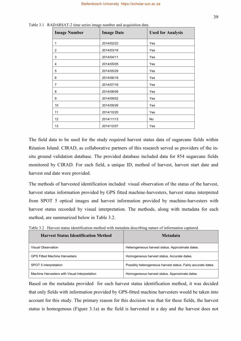
39

Table 3.1 RADARSAT-2 time series image number and acquisition date.

Image Number Image Date Used for Analysis

1 2014/02/22 Yes

2 2014/03/18 Yes

3 2014/04/11 Yes

4 2014/05/05 Yes

5 2014/05/29 Yes

6 2014/06/18 Yes

7 2014/07/16 Yes

8 2014/08/09 Yes

9 2014/09/02 Yes

10 2014/09/26 Yes

11 2014/10/20 Yes

12 2014/11/13 No

13 2014/12/07 Yes

The field data to be used for the study required harvest status data of sugarcane fields within

Rèunion Island. CIRAD, as collaborative partners of this research served as providers of the in-

situ ground validation database. The provided database included data for 854 sugarcane fields

monitored by CIRAD. For each field, a unique ID, method of harvest, harvest start date and

harvest end date were provided.

The methods of harvested identification included: visual observation of the status of the harvest,

harvest status information provided by GPS fitted machine-harvesters, harvest status interpreted

from SPOT 5 optical images and harvest information provided by machine-harvesters with

harvest status recorded by visual interpretation. The methods, along with metadata for each

method, are summarized below in Table 3.2.

Table 3.2 Harvest status identification method with metadata describing nature of information captured.

Harvest Status Identification Method Metadata

Visual Observation Heterogeneous harvest status. Approximate dates.

GPS Fitted Machine Harvesters Homogeneous harvest status. Accurate dates.

SPOT 5 interpretation Possibly heterogeneous harvest status. Fairly accurate dates.

Machine Harvesters with Visual Interpretation Homogeneous harvest status. Approximate dates.

Based on the metadata provided for each harvest status identification method, it was decided

that only fields with information provided by GPS-fitted machine harvesters would be taken into

account for this study. The primary reason for this decision was that for these fields, the harvest

status is homogenous (Figure 3.1a) as the field is harvested in a day and the harvest does not


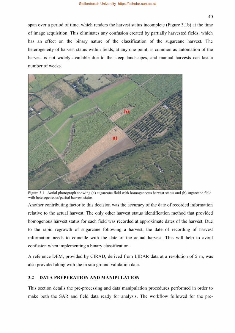
40

span over a period of time, which renders the harvest status incomplete (Figure 3.1b) at the time

of image acquisition. This eliminates any confusion created by partially harvested fields, which

has an effect on the binary nature of the classification of the sugarcane harvest. The

heterogeneity of harvest status within fields, at any one point, is common as automation of the

harvest is not widely available due to the steep landscapes, and manual harvests can last a

number of weeks.

Figure 3.1 Aerial photograph showing (a) sugarcane field with homogeneous harvest status and (b) sugarcane field

with heterogeneous/partial harvest status.

Another contributing factor to this decision was the accuracy of the date of recorded information

relative to the actual harvest. The only other harvest status identification method that provided

homogenous harvest status for each field was recorded at approximate dates of the harvest. Due

to the rapid regrowth of sugarcane following a harvest, the date of recording of harvest

information needs to coincide with the date of the actual harvest. This will help to avoid

confusion when implementing a binary classification.

A reference DEM, provided by CIRAD, derived from LIDAR data at a resolution of 5 m, was

also provided along with the in situ ground validation data.

3.2 DATA PREPERATION AND MANIPULATION

This section details the pre-processing and data manipulation procedures performed in order to

make both the SAR and field data ready for analysis. The workflow followed for the pre-

b)

a)


41

processing of the imagery is outlined in Figure 3.2 and discussed in detail in the succeeding

sections of this chapter.

Figure 3.2 Pre-processing workflow for preparation of RADARSAT-2 imagery.

The nature of the study, relating to Experiment 1 and 2, required that pre-processing of the

backscatter bands be undertaken following two different methods, as explained in the section to

follow (3.2.1).

3.2.1 Pre-processing the backscatter bands

To account for the distortions inherent in range-based SAR systems, terrain geocoding was

performed for each of the backscatter bands. The geocoding and terrain correction were

performed using the SARScape extension in ENVI (V5.2.0). A reference DEM, provided by

CIRAD, derived from LIDAR data at a resolution of 5 m, was used to correct each image

position to a geodetic position on the earth’s surface. The process of geocoding also accounted

for radiometric calibration using the local incidence angle, where the image backscatter values

were transformed to sigma-0. Sigma-0, measured in decibels (dB), allowed the true backscatter

values of the reflecting surface to be represented and, therefore, proved ideal for the quantitative

nature of the study.


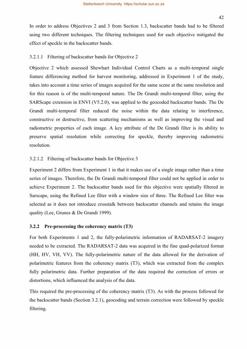
42

In order to address Objectives 2 and 3 from Section 1.3, backscatter bands had to be filtered

using two different techniques. The filtering techniques used for each objective mitigated the

effect of speckle in the backscatter bands.

3.2.1.1 Filtering of backscatter bands for Objective 2

Objective 2 which assessed Shewhart Individual Control Charts as a multi-temporal single

feature differencing method for harvest monitoring, addressed in Experiment 1 of the study,

takes into account a time series of images acquired for the same scene at the same resolution and

for this reason is of the multi-temporal nature. The De Grandi multi-temporal filter, using the

SARScape extension in ENVI (V5.2.0), was applied to the geocoded backscatter bands. The De

Grandi multi-temporal filter reduced the noise within the data relating to interference,

constructive or destructive, from scattering mechanisms as well as improving the visual and

radiometric properties of each image. A key attribute of the De Grandi filter is its ability to

preserve spatial resolution while correcting for speckle, thereby improving radiometric

resolution.

3.2.1.2 Filtering of backscatter bands for Objective 3

Experiment 2 differs from Experiment 1 in that it makes use of a single image rather than a time

series of images. Therefore, the De Grandi multi-temporal filter could not be applied in order to

achieve Experiment 2. The backscatter bands used for this objective were spatially filtered in

Sarscape, using the Refined Lee filter with a window size of three. The Refined Lee filter was

selected as it does not introduce crosstalk between backscatter channels and retains the image

quality (Lee, Grunes & De Grandi 1999).

3.2.2 Pre-processing the coherency matrix (T3)

For both Experiments 1 and 2, the fully-polarimetric information of RADARSAT-2 imagery

needed to be extracted. The RADARSAT-2 data was acquired in the fine quad-polarized format

(HH, HV, VH, VV). The fully-polarimetric nature of the data allowed for the derivation of

polarimetric features from the coherency matrix (T3), which was extracted from the complex

fully polarimetric data. Further preparation of the data required the correction of errors or

distortions, which influenced the analysis of the data.

This required the pre-processing of the coherency matrix (T3). As with the process followed for

the backscatter bands (Section 3.2.1), geocoding and terrain correction were followed by speckle

filtering.


43

Geocoding and terrain correction of the T3 matrix for individual images was performed using

ASF MapReady (V 3.1.24) with the reference DEM provided by CIRAD. The outputs were

exported in PolSARpro format for further pre-processing. Upon investigation, it was noted that

an error, in the form of a longitude coordinate error, occurred in the writing of the header files

following geocoding in MapReady. Each of the header files were manually corrected.

As with the backscatter bands, the T3 matrix contains inherent noise known as speckle which

appears as a grainy salt-and-pepper effect on the images. Filtering was performed on the T3

matrix in order to reduce speckle. In order to maintain the full polarimetric phase information

available for each image, a spatial filter, specifically a polarimetric spatial filter, was used.

Filtering was performed using PolSARpro (V4.2.0), which has a number of spatial filters

available. Literature suggests the use of either the Boxcar filter or the Refined Lee filter (Qi et al.

2012). However, the boxcar filter available was not used as it reduces speckle by averaging the

intensity of neighbouring pixels. Therefore, the noise is smoothed and spatial resolution is lost

(Ferro-Famil, Pottier & Lee 2011). As suggested by literature, the Refined Lee filter was used

(Qi et al. 2012). It emphasises preserving polarimetric properties and statistical correlations

between channels, doesn’t introduce crosstalk and doesn’t degrade the image quality (Lee,

Grunes & de Grandi 1999). Speckle filtering with a moving window size of 3x3 was used.

Selection of the window size was based on visual investigation of outputs with varying window

sizes.

3.2.3 Ground truth database

In situ ground validation data is important for training and validation of supervised and machine

learning classification algorithms. A ground validation database traditionally consists of

information acquired during visits to the field in order to accurately record the true earth

conditions at the time of image acquisition. However, due to restrictions in access and those

relating to financial restrictions, it is not always possible to undertake these field visits.

CIRAD, as collaborative partners of this research served as providers of the in-situ ground

validation database. The study required harvest status data of sugarcane fields within Rèunion

Island. The provided database included data for 854 sugarcane fields monitored by CIRAD. For

each field, a unique ID, method of harvest, harvest start date and harvest end date were provided.

Data cleaning was then conducted on the provided database in order to refine the ground

validation data to fit the needs of the study. Following the selection of the fields only harvested

using GPS-fitted machine harvesters, the field database was clipped to the extent of the

RADARSAT-2 imagery. A total of 65 fields remained available for analysis.


44

The ground validation database was used as both a training and validation database.

3.2.4 Feature extraction

Following the pre-processing of the image data as well as the data cleaning of the ground truth

database, further processing was required. A collection of image derivatives, or image features,

were extracted from the fully polarimetric data. These features can then be used to train a

classification algorithm as well as create threshold values to classify objects. In the case of this

study, these are harvested and unharvested sugarcane fields. The features that are derived depend

on the type of data to be used for analysis. These features often include ratios and statistical

measures of information inherent in the imagery. The nature of these features is dependent on the

study, and no bounds can be put on which features to derive for a particular application. The

features extracted for the purpose of this study comprised of backscatter, polarimetric

decomposition parameters, ratios and texture measures.

3.2.4.1 Polarimetric Information

The fully polarimetric nature of the imagery allows for decomposition into different scattering

components in order to either enhance or suppress the contribution from a particular scattering

mechanism (Van Zyl, Arii & Kim 2011). These decompositions were used in addressing both

Objectives 2 and 3 of the study. The decompositions were extracted using the PolSARpro

(V4.2.0) software. The extraction process required the specification of a window size to be used

when estimating the polarimetric parameters. A window size of one was selected applying no

averaging to the data.

Five decompositions were extracted, each consisting of parameters that aim to explain the

contribution of particular scattering mechanisms on the earths’ surface. The decompositions and

features produced by each are summarized below in Table 3.3. The mean value of each of these

features (per field) was used a representative value.

Table 3.3 Polarimetric decompositions along with radar features extracted

Cloude-Pottier Freeman-Durden Krogager Van Zyl Yamaguchi

Entropy Volume Scattering Helix Volume Scattering Volume Scattering

Anisotropy Double Bounce Sphere Double Bounce Double Bounce

Alpha Odd bounce Diplane Odd bounce Odd bounce

Helix Scattering

The extraction of these polarimetric features added dimensionality to the existing dataset of

backscatter bands. All polarimetric features and backscatter channels (HH, HV and VV) were


45

extracted for data analysis, which included moving range control curves, feature selection and

object-based image classification methods.

3.2.4.2 Image texture

Image texture is defined as a measure of the variation in the intensity of a surface. Information

contained within the texture measures aid in explaining the arrangement of objects and their

spatial relationships. Features derived from texture considerably increase the dimensionality of

the dataset and, therefore, were only implemented for use in single image classification

(Experiment 2) where feature selection was used for dimensionality reduction.

Since texture features were only used in Experiment 2, single-image classification, texture

measures were only calculated for one image date (12/07/2014). Texture measures were

extracted from each of the 19 previously derived layers (16 decomposition features and 3

backscatter channels) for each of the 65 sugarcane fields. It should be noted that the backscatter

channels from which texture features were extracted were spatially filtered, as described in

Section 3.2.1.2. Texture features were derived from both the Grey Level Co-occurrence Matrix

(GLCM) and the Grey Level Difference Vector (GLDV). The extraction of these textures was

performed using eCognition (V9.0.3). The selected software required that a segmentation step be

performed to identify objects for which the textures features were to be extracted. A shapefile

containing the field boundaries of the 65 sugarcane fields was used as a thematic layer and,

therefore, the scale parameter for chessboard segmentation was set to create an object

encompassing the image. This allowed for only the fields specified by the thematic layer to be

identified as objects from which texture could be derived. A total of 12 texture measures were

derived for each of the 19 image layers previously extracted, and these texture measures are

presented in Table 3.4.


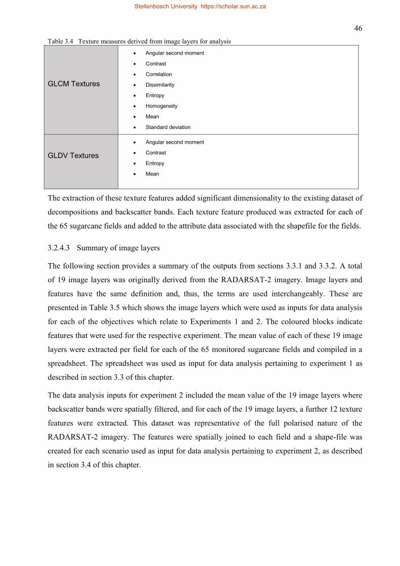
46

Table 3.4 Texture measures derived from image layers for analysis

GLCM Textures

Angular second moment

Contrast

Correlation

Dissimilarity

Entropy

Homogeneity

Mean

Standard deviation

GLDV Textures

Angular second moment

Contrast

Entropy

Mean

The extraction of these texture features added significant dimensionality to the existing dataset of

decompositions and backscatter bands. Each texture feature produced was extracted for each of

the 65 sugarcane fields and added to the attribute data associated with the shapefile for the fields.

3.2.4.3 Summary of image layers

The following section provides a summary of the outputs from sections 3.3.1 and 3.3.2. A total

of 19 image layers was originally derived from the RADARSAT-2 imagery. Image layers and

features have the same definition and, thus, the terms are used interchangeably. These are

presented in Table 3.5 which shows the image layers which were used as inputs for data analysis

for each of the objectives which relate to Experiments 1 and 2. The coloured blocks indicate

features that were used for the respective experiment. The mean value of each of these 19 image

layers were extracted per field for each of the 65 monitored sugarcane fields and compiled in a

spreadsheet. The spreadsheet was used as input for data analysis pertaining to experiment 1 as

described in section 3.3 of this chapter.

The data analysis inputs for experiment 2 included the mean value of the 19 image layers where

backscatter bands were spatially filtered, and for each of the 19 image layers, a further 12 texture

features were extracted. This dataset was representative of the full polarised nature of the

RADARSAT-2 imagery. The features were spatially joined to each field and a shape-file was

created for each scenario used as input for data analysis pertaining to experiment 2, as described

in section 3.4 of this chapter.


47

Table 3.5 Summary of image layers to be used for Experiments 1 and 2.

Feature name Experiment 1 Experiment 2

HH Backscatter (De Grandi Multi-temporal filter) X

HV Backscatter (De Grandi Multi-temporal filter) X

VV Backscatter (De Grandi Multi-temporal filter) X

HH Backscatter (Refined Lee Spatial filter) X

HV Backscatter (Refined Lee Spatial filter) X

VV Backscatter (Refined Lee Spatial filter) X

Freeman-Durden Volume Scattering X X

Freeman-Durden Double Bounce X X

Freeman-Durden Odd bounce X X

Krogager Helix X X

Krogager Sphere X X

Krogager Diplane X X

Van Zyl Volume Scattering X X

Van Zyl Double Bounce X X

Van Zyl Odd bounce X X

Yamaguchi Double Bounce X X

Yamaguchi Odd bounce X X

Yamaguchi Helix Scattering X X

Yamaguchi Volume Scattering X X

Texture measures X

Another dataset, in order to answer research questions derived from Objective 3, was

representative of the simulated dual polarised scenario. For the simulated dual polarised scenario,

only the VV and HV backscatter image layers were included, and from these image layers,

textures were also extracted, and a ratio between VV and HV was created. Again, each of the

values were extracted per field for the 65 sugarcane fields been monitored. For the fully

polarimetric dataset, a total of 247 features was thus extracted per field and for the simulated

dual polarimetric scenario, there were 27 features.

3.3 EXPERIMENT 1: SINGLE FEATURE HARVEST MONITORING

The method used for harvest monitoring in this experiment is a form of statistical quality control.

Traditionally, the method, proposed by Walter Shewhart in the 1920s, was used in controlling

the variance in manufacturing processes and became known as the Shewhart individual control

chart.


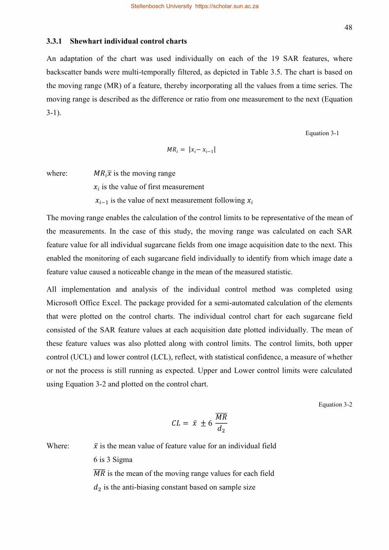
48

3.3.1 Shewhart individual control charts

An adaptation of the chart was used individually on each of the 19 SAR features, where

backscatter bands were multi-temporally filtered, as depicted in Table 3.5. The chart is based on

the moving range (MR) of a feature, thereby incorporating all the values from a time series. The

moving range is described as the difference or ratio from one measurement to the next (Equation

3-1).

Equation 3-1

𝑀𝑅𝑖 = |𝑥𝑖− 𝑥𝑖−1|

where: 𝑀𝑅𝑖�̅� is the moving range

𝑥𝑖 is the value of first measurement

𝑥𝑖−1 is the value of next measurement following 𝑥𝑖

The moving range enables the calculation of the control limits to be representative of the mean of

the measurements. In the case of this study, the moving range was calculated on each SAR

feature value for all individual sugarcane fields from one image acquisition date to the next. This

enabled the monitoring of each sugarcane field individually to identify from which image date a

feature value caused a noticeable change in the mean of the measured statistic.

All implementation and analysis of the individual control method was completed using

Microsoft Office Excel. The package provided for a semi-automated calculation of the elements

that were plotted on the control charts. The individual control chart for each sugarcane field

consisted of the SAR feature values at each acquisition date plotted individually. The mean of

these feature values was also plotted along with control limits. The control limits, both upper

control (UCL) and lower control (LCL), reflect, with statistical confidence, a measure of whether

or not the process is still running as expected. Upper and Lower control limits were calculated

using Equation 3-2 and plotted on the control chart.

Equation 3-2

𝐶𝐿 = �̅� ± 6 𝑀𝑅̅̅ ̅̅̅

𝑑2

Where: �̅� is the mean value of feature value for an individual field

6 is 3 Sigma

𝑀𝑅̅̅̅̅̅ is the mean of the moving range values for each field

𝑑2 is the anti-biasing constant based on sample size


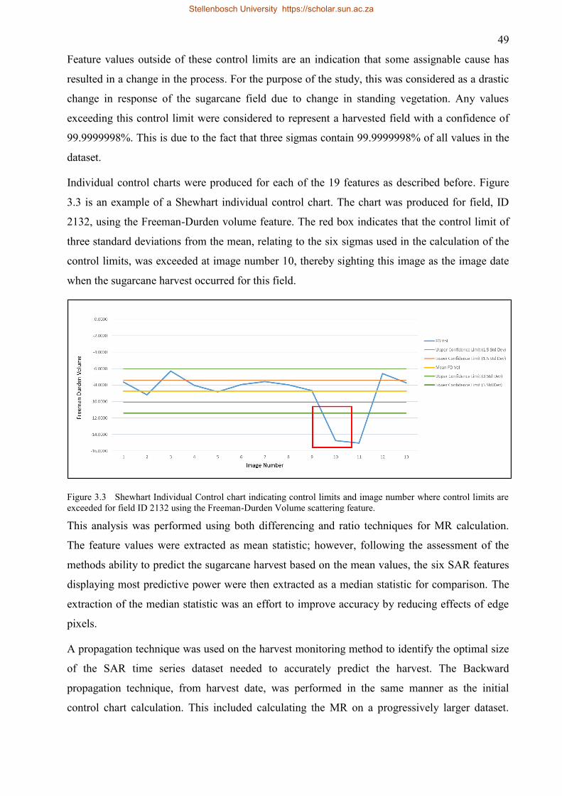
49

Feature values outside of these control limits are an indication that some assignable cause has

resulted in a change in the process. For the purpose of the study, this was considered as a drastic

change in response of the sugarcane field due to change in standing vegetation. Any values

exceeding this control limit were considered to represent a harvested field with a confidence of

99.9999998%. This is due to the fact that three sigmas contain 99.9999998% of all values in the

dataset.

Individual control charts were produced for each of the 19 features as described before. Figure

3.3 is an example of a Shewhart individual control chart. The chart was produced for field, ID

2132, using the Freeman-Durden volume feature. The red box indicates that the control limit of

three standard deviations from the mean, relating to the six sigmas used in the calculation of the

control limits, was exceeded at image number 10, thereby sighting this image as the image date

when the sugarcane harvest occurred for this field.

Figure 3.3 Shewhart Individual Control chart indicating control limits and image number where control limits are

exceeded for field ID 2132 using the Freeman-Durden Volume scattering feature.

This analysis was performed using both differencing and ratio techniques for MR calculation.

The feature values were extracted as mean statistic; however, following the assessment of the

methods ability to predict the sugarcane harvest based on the mean values, the six SAR features

displaying most predictive power were then extracted as a median statistic for comparison. The

extraction of the median statistic was an effort to improve accuracy by reducing effects of edge

pixels.

A propagation technique was used on the harvest monitoring method to identify the optimal size

of the SAR time series dataset needed to accurately predict the harvest. The Backward

propagation technique, from harvest date, was performed in the same manner as the initial

control chart calculation. This included calculating the MR on a progressively larger dataset.


50

When calculating the control limits the anti-biasing constant needed change with the addition of

each SAR image added to the dataset as it is a constant based specifically on dataset size.

3.3.2 Shewhart individual control charts accuracy assessment

The accuracy of the harvest monitoring was based on harvest date as recorded by the CIRAD

sugarcane harvest monitoring database. Two sets of complementary accuracy tests were

performed. The first took into account only the correct flagging of the harvest. I.e. was the

control limit exceeded on the correct image acquisition date in relation to the harvest monitoring

database. Hereby identifying the percentage of fields for which harvest date was correctly

identified.

The second was in the form of a confusion matrix. This allowed for the calculation of errors of

omission and commission. The confusion matrices were only assessed for the six best

performing features based on the initial accuracy of harvest flagging. The first accuracy

assessment mentioned was implemented based on the fact that the number of true negatives

(image dates in which a particular field is unharvested) far outweighed the number of true

positives (image dates on which a particular field is harvested) and, for this reason, could cause

an imbalance in the overall accuracy calculated by the error matrix. Each of the accuracy

assessments were performed on 60 homogenous sugarcane fields individually and not the initial

65 homogenous sugarcane fields mentioned. The reason for this is that five of the sugarcane

fields were harvested during the acquisition of image number 12 (acquired on 13/11/2014) which

was not used in analysis due to calibration issues. The results of the data analysis from this

section, along with an in-depth discussion based on the results, are presented in Section

CHAPTER 4: .

3.4 EXPERIMENT 2: SINGLE IMAGE HARVEST CLASSIFICATION

In order to achieve Objective 3 which aimed to assess different machine learning classifiers,

applied to single-date, dual- and quad-polarized imagery, single date object-based image

classification was undertaken. This allowed for determining the relative value of fully

polarimetric features as opposed to a simple dual-pol backscatter case. Due to the large number

of features derived as input for this method of data analysis it was required that feature selection

be undertaken prior to single date object-based image classification.

3.4.1 Feature selection

The dimensionality of the input dataset for single date object-based image classification was

deemed too complex for the classification methods that were to be tested. The 247 fully


51

polarimetric and the 27 simulated dual polarimetric object features derived (Table 3.5) had to be

reduced through the process of feature selection. Due to the range of classifiers to be tested, it

was decided that a filter approach be used as a feature selection technique rather than a wrapper

approach found embedded within selected classifiers. This decision allowed for a standardised

base of feature selection prior to classification. The method used for feature selection was a two-

tiered operation whereby Explanatory Factor Analysis (EFA) was followed by one-way Analysis

of Variance (ANOVA). The use of such a multi-tiered method provided for a more robust feature

selection method.

3.4.1.1 Exploratory Factor Analysis

EFA was performed using a statistical software package, Statistica, and is heuristic in nature.

EFA aims to describe the variability among observed variables in terms of a reduced number of

unobserved variables known as factors. Linear combinations of these factors were used to model

the observed variable, thereby estimating how much of the variability in the data was as a result

of the common factors. The factors contained the image features used as input and depicted how

much variance they contributed when modelling the observed variable, in the case of this study,

the harvest status. The decision on how many factors to select when reducing the dimensionality

of the data was reached through the use of a Scree plot (Figure 3.4). A scree plot plots the

amount of variability, within the observed variable, contributed by each of the factors. As

suggested by literature, the natural bend in the curve was found (Figure 3.4), and the number of

data points or factors plotted above this bend were retained.


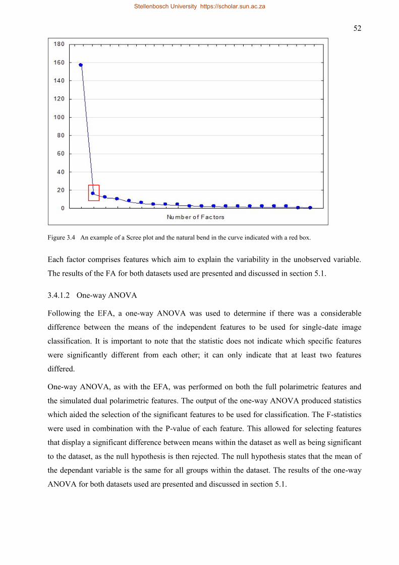
52

Figure 3.4 An example of a Scree plot and the natural bend in the curve indicated with a red box.

Each factor comprises features which aim to explain the variability in the unobserved variable.

The results of the FA for both datasets used are presented and discussed in section 5.1.

3.4.1.2 One-way ANOVA

Following the EFA, a one-way ANOVA was used to determine if there was a considerable

difference between the means of the independent features to be used for single-date image

classification. It is important to note that the statistic does not indicate which specific features

were significantly different from each other; it can only indicate that at least two features

differed.

One-way ANOVA, as with the EFA, was performed on both the full polarimetric features and

the simulated dual polarimetric features. The output of the one-way ANOVA produced statistics

which aided the selection of the significant features to be used for classification. The F-statistics

were used in combination with the P-value of each feature. This allowed for selecting features

that display a significant difference between means within the dataset as well as being significant

to the dataset, as the null hypothesis is then rejected. The null hypothesis states that the mean of

the dependant variable is the same for all groups within the dataset. The results of the one-way

ANOVA for both datasets used are presented and discussed in section 5.1.


53

3.4.2 Image classification

Following feature selection, the reduced number of features were then used to classify a single

image, image number 13 (12/07/2014). The classification was performed on image number 13

(07/12/2014) as the number of and spread between harvested and unharvested sugarcane fields

was even and allowed for suitable training data. The classification was binary, aiming to identify

harvested and unharvested sugarcane fields within predetermined field boundaries. The

Supervised Learning and Image Classification Environment (SLICE) software developed by the

Centre for Geographical Analysis (CGA) at Stellenbosch Univeristy was used for classification

and accuracy assessment.

The SLICE software was developed using the C++ programming language and makes use of

external libraries for various classifiers and for generating shapefile outputs. Six classification

algorithms were assessed for sugarcane harvest classification, five of which made use of

OpenCV libraries (Bradski & Pisarevsky 2000) while the remaining classification was

implemented using the Libsvm library (Chang & Lin 2011). These included K-Nearest

Neighbour (KNN), where k was set to 1, as suggested by Qian et al. (2015), Decision Trees

(DT), Random Trees (RT), Support Vector Machines (SVM) and Maximum Likelihood (ML)

and a second SVM classification using Libsvm (Chang & Lin 2011). Due to the nature of the

software, which randomises the data such that for each iteration of classification, different

samples are used for training and validation, 10 iterations for each classification were completed.

In order to quantify the effect of using fully-polarimetric data, compared to a simulated dual

polarimetric dataset, classifications were performed on both datasets for image 13, and

accuracies for each were determined. For the fully polarised dataset, the mean value of the 19

image layers was used, and for each of the 19 image layers, a further 12 texture features were

extracted. This dataset was representative of the full polarised nature of the RADARSAT-2

imagery. Each of the values were extracted per field for the 65 sugarcane fields monitored. The

fully polarimetric dataset contained a total of 247 features which were used for classification.

The dual polarised scenario using only the HV and VV backscatter image layers were included.

For both the HV and VV backscatter image layers, textures were also extracted, and a ratio

between HV and VV was created. The simulated dual polarimetric scenario had 27 features to be

used for classification.

Image classification were also performed at each level of feature selection, including the initial

stage where all features were used. This allowed for assessing the validity of the selected feature

selection technique. The results for the data analysis from this section, along with an in-depth

discussion based on the results, are presented in Section CHAPTER 5: of Chapter 4.


54

3.4.3 Classification accuracy

In order to assess the accuracy of the classification the 65 fields were split into training and

validation datasets for classification. The training dataset comprised 60% (39) of the fields, while

the validation data comprised the remaining 40% (26). The SLICE software used for classifying

the images randomises the data such that for each iteration of classification, different samples are

used for training and validation. The classification software used has a built-in feature whereby

confusion matrices, overall accuracies (OA) and the kappa coefficients (K) for each

classification iteration are produced. Kappa values greater than 0.7 were deemed as good (Fleiss

1981). This made the interpretation of classification results simple as the information needed for

assessing single image object-based classification was clearly presented. A total of 10 iterations

of each classification was performed, and the final results were averaged to get a more accurate

representation of the classifiers’ ability to identify harvested and unharvested fields. The results,

as presented in Section CHAPTER 5: , help to determine the effectiveness of obtaining and

implementing a fully polarimetric dataset, as opposed to a dual polarimetric dataset for

individual image harvest classification. This aids in addressing the research questions associated

with Objective 3 in Section 1.1 of this thesis.

CHAPTER 4: and CHAPTER 5: following this section present, and analytically discusses the

results of Experiment 1 and Experiment 2 respectively.


55

CHAPTER 4: RESULTS AND DISCUSSION EXPERIMENT 1

The aim of this experiment was to evaluate Shewhart Individual Control Charts as a multi-

temporal single feature differencing method for harvest monitoring and determine how many

RADARSAT-2 images are required for multi-temporal single feature harvest monitoring.

In order for the above-mentioned aim to be achieved, the following research questions were

addressed:

1. What is the effectiveness of a multi-temporal single feature differencing method for

harvest monitoring?

2. What is the appropriate size of the multi-temporal dataset required for achieving peak

harvest detection accuracy?

This experiment used a time-series of 12 images to construct Shewhart individual control charts

in order to detect (per field) the date on which harvest occurred in that field. Values for each of

the 19 SAR features were extracted for each GPS-monitored sugarcane cane field, of which there

were 60 from each image date.

The results for experiment 1 are presented in the following order: first, the accuracies from the

Shewhart individual control chart for each SAR feature, based on the mean value of each feature,

for each sugarcane field are presented and discussed (Section 4.1). Following from this, the top

six performing features from the first experiment are then assessed whereby a median value for

each field, instead of the mean value, was used (Section 4.2.1). A comparison of feature

accuracies is then made when the MR was calculated using a ratio technique, as opposed to a

differencing technique (Section 4.2.2).This allowed for continuation into the next part of the

experiment (Section 4.2.3) where the appropriate size of the multi-temporal dataset required for

achieving peak harvest detection accuracy was tested.

4.1 Shewhart individual control charts based on mean value

The Shewhart individual control charts, using the mean value for each sugarcane field for each

feature, accuracies were assessed based on the CIRAD sugarcane harvest monitoring database.

Two sets of complementing accuracy tests were performed. The first focused on individual

features to be used for harvest detection only while the second complemented this by validating

the individual features to be applicable for harvest monitoring.


56

4.1.1 Harvest detection

The first took into account only the flagging or identification of the harvest; was the control limit

exceeded on the correct image acquisition date in relation to the harvest monitoring database.

The harvest identification accuracy results based on the mean value across all sugarcane fields

for each feature are presented in Figure 4.1. The figure presents the accuracy with which each

SAR feature is able to predict the sugarcane harvest date for each field.

Figure 4.1 SAR features and their accuracies for sugarcane harvest detection

The above figure represents the results in order of highest accuracy achieved by features used in

for Shewhart individual control charts.

The results shown in Figure 4.1 indicate that the volume components from the polarimetric

decompositions achieve the highest sugarcane harvest detection accuracies, with Freeman-

Durden volume (88.33%), Van Zyl volume (86.67%) and Yamaguchi volume (85.00%)

components displaying the greatest predictive powers. The Krogager diplane (Kd) component

(83.33%), which also relates to the volume scattering component, displays slightly lower harvest

identification abilities. This can be credited to the fact that the Krogager decomposition is a

coherent decomposition. Coherent decompositions express the scattering matrix measured by the

radar as the combination of the scattering responses of simpler objects and are thus able to

characterise the scattering process produced by a given target (POLSAR Pro v5.0.3). In contrast

to this, incoherent decompositions, those displaying greater predictive ability, are able to


57

describe a complex target as opposed to a target where there is a single dominant scatterer (Lee

& Pottier 2009).

The backscatter channels displaying the greatest sugarcane harvest detection capabilities are the

HV (80.00%) and VV (80.00%) channels. The high accuracies achieved by these features can be

attributed to the scattering measured by the cross- polarization channel (HV) and this channels

ability for vegetation mapping, specifically sugarcane harvest mapping, as identified by

Baghdadi et al. (2009). Multiple scattering within the vegetation volume are related to the

altering of the polarization.

The volume components of the decompositions were able identify the sugarcane harvest with

greater accuracy as volume scattering is greater in vegetation. This is due to volume scattering

being modelled as a contribution from a cloud of randomly orientated cylinder-like scatterers,

which are dominant in vegetation. These results are in accordance with Li et al.’s (2012) study

which identified the Freeman-Durden volume scattering component to be stable throughout the

growing season until harvest, when there was a noticeable decline.

The accuracies achieved in Figure 4.1 are only representative of the features’ abilities to detect

the image closest to the harvest date rather than accurately monitor the harvest throughout a

sugarcane growing season.

4.1.2 Harvest monitoring

Following from the first method of accuracy evaluation described as sugarcane harvest detection,

the second method of assessing accuracy was in the form of a confusion matrix. This allowed for

the calculation of errors of omission and commission. By calculating the errors of commission

and omission, the method now monitors the harvest rather than only detecting the harvest. Each

of the best six features (Freeman Durden Volume, Van Zyl Volume, Yamaguchi Volume,

Krogager Kd, HV backscatter and VV Backscatter) identified from the harvest detection

accuracy were analysed, and confusion matrices were produced for each. The confusion matrices

allowed for the calculation of error of commission, error of omission and overall accuracy. Table

4.1 shows an example of a calculated confusion matrix for the Freeman-Durden volume

scattering component. All matrices calculated are included in Appendix A.


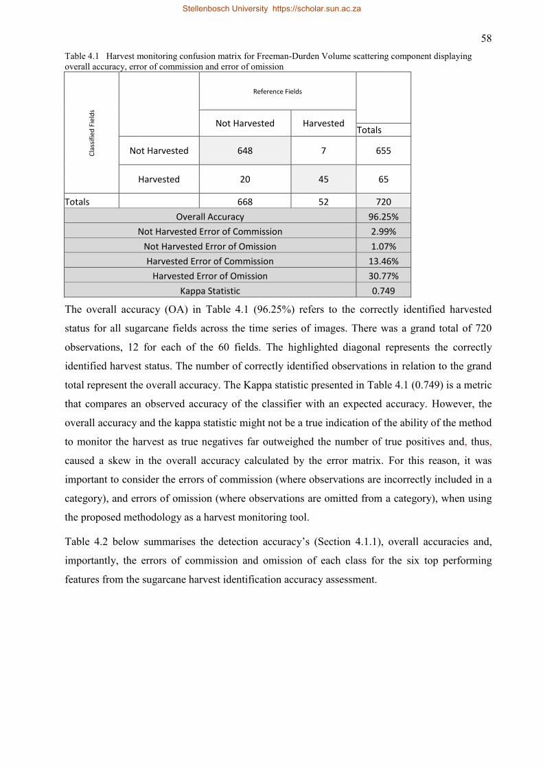
58

Table 4.1 Harvest monitoring confusion matrix for Freeman-Durden Volume scattering component displaying

overall accuracy, error of commission and error of omission

Cla

ssif

ied

Fie

lds

Reference Fields

Not Harvested Harvested

Totals

Not Harvested 648 7 655

Harvested 20 45 65

Totals 668 52 720

Overall Accuracy 96.25%

Not Harvested Error of Commission 2.99%

Not Harvested Error of Omission 1.07%

Harvested Error of Commission 13.46%

Harvested Error of Omission 30.77%

Kappa Statistic 0.749

The overall accuracy (OA) in Table 4.1 (96.25%) refers to the correctly identified harvested

status for all sugarcane fields across the time series of images. There was a grand total of 720

observations, 12 for each of the 60 fields. The highlighted diagonal represents the correctly

identified harvest status. The number of correctly identified observations in relation to the grand

total represent the overall accuracy. The Kappa statistic presented in Table 4.1 (0.749) is a metric

that compares an observed accuracy of the classifier with an expected accuracy. However, the

overall accuracy and the kappa statistic might not be a true indication of the ability of the method

to monitor the harvest as true negatives far outweighed the number of true positives and, thus,

caused a skew in the overall accuracy calculated by the error matrix. For this reason, it was

important to consider the errors of commission (where observations are incorrectly included in a

category), and errors of omission (where observations are omitted from a category), when using

the proposed methodology as a harvest monitoring tool.

Table 4.2 below summarises the detection accuracy’s (Section 4.1.1), overall accuracies and,

importantly, the errors of commission and omission of each class for the six top performing

features from the sugarcane harvest identification accuracy assessment.


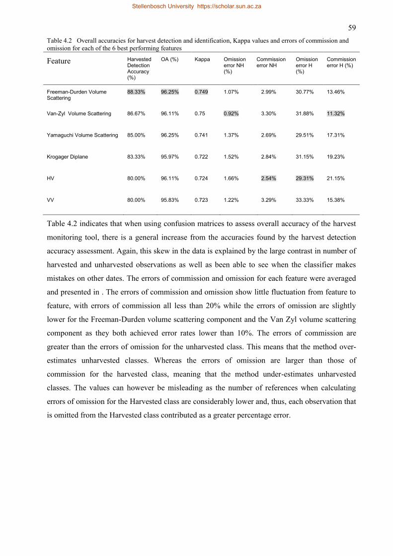
59

Table 4.2 Overall accuracies for harvest detection and identification, Kappa values and errors of commission and

omission for each of the 6 best performing features

Feature Harvested Detection Accuracy (%)

OA (%) Kappa Omission error NH (%)

Commission error NH

Omission error H (%)

Commission error H (%)

Freeman-Durden Volume Scattering

88.33% 96.25% 0.749 1.07% 2.99% 30.77% 13.46%

Van-Zyl Volume Scattering 86.67% 96.11% 0.75 0.92% 3.30% 31.88% 11.32%

Yamaguchi Volume Scattering 85.00% 96.25% 0.741 1.37% 2.69% 29.51% 17.31%

Krogager Diplane 83.33% 95.97% 0.722 1.52% 2.84% 31.15% 19.23%

HV 80.00% 96.11% 0.724 1.66% 2.54% 29.31% 21.15%

VV 80.00% 95.83% 0.723 1.22% 3.29% 33.33% 15.38%

Table 4.2 indicates that when using confusion matrices to assess overall accuracy of the harvest

monitoring tool, there is a general increase from the accuracies found by the harvest detection

accuracy assessment. Again, this skew in the data is explained by the large contrast in number of

harvested and unharvested observations as well as been able to see when the classifier makes

mistakes on other dates. The errors of commission and omission for each feature were averaged

and presented in . The errors of commission and omission show little fluctuation from feature to

feature, with errors of commission all less than 20% while the errors of omission are slightly

lower for the Freeman-Durden volume scattering component and the Van Zyl volume scattering

component as they both achieved error rates lower than 10%. The errors of commission are

greater than the errors of omission for the unharvested class. This means that the method over-

estimates unharvested classes. Whereas the errors of omission are larger than those of

commission for the harvested class, meaning that the method under-estimates unharvested

classes. The values can however be misleading as the number of references when calculating

errors of omission for the Harvested class are considerably lower and, thus, each observation that

is omitted from the Harvested class contributed as a greater percentage error.


60

Figure 4.2 Averaged errors of commission and omission for each of the 6 best performing features

The errors of commission and omission are relatively constant across all features, indicating that

the method is robust across individual features when using Shewhart individual control charts for

harvest monitoring.

Baghdadi et al. (2009) identified the HV backscatter channel as having potential for harvest

monitoring, specifically sugarcane harvest mapping, as the multiple scattering within the

vegetation volume are related to the altering of the polarization. This is in agreement with the

harvest identification accuracy for HV backscatter in Figure 4.1, complemented by the results in

Table 4.2 and Figure 4.2, where the sugarcane harvest status was consistently accurately

identified with an average error of less than 20% for both errors of omission and commission.

4.2 Improving Shewhart individual control chart accuracy

Section 4.1 focused on identifying the best features for use in harvest detection and monitoring.

The six features identified were then used in experiments that evaluated the effect of mean vs

median and difference vs ratio to see if it improves the accuracy achieved using Shewhart

individual control charts and variations thereof.

4.2.1 Comparison between mean and median field values

When extracting feature values for each field, the mean statistic of each field was initially used.

However, this statistic can be misleading when extracting feature values as pixels along the edge

of the fields are not representative of what the field is composed of. Therefore, it was important

to test the effect of excluding these outlying pixels. The median value is the midpoint of a


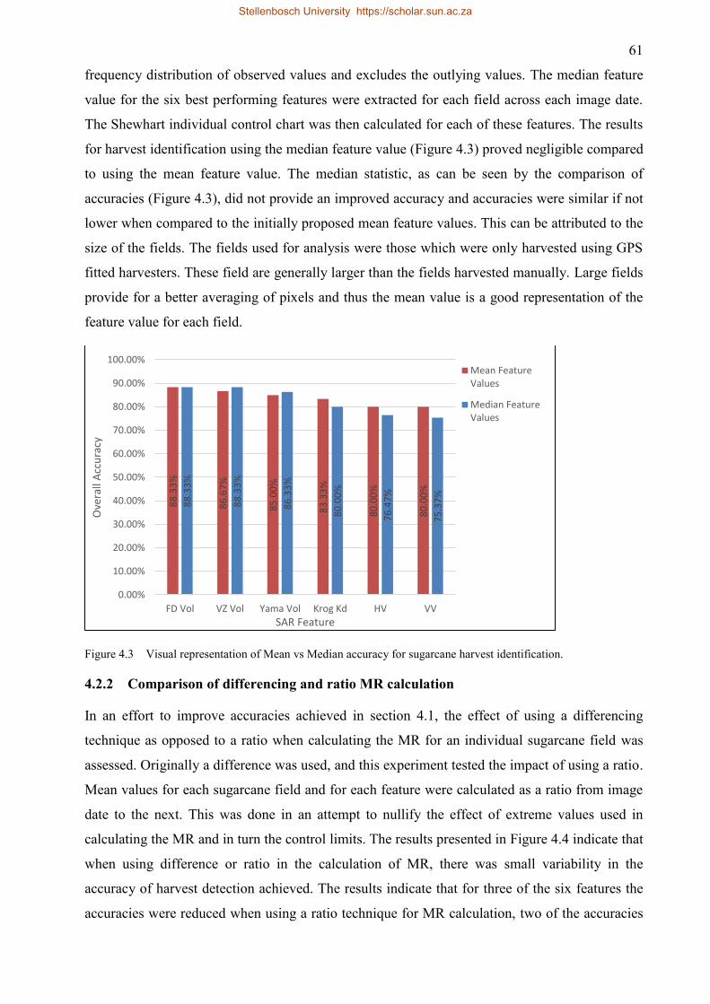
61

frequency distribution of observed values and excludes the outlying values. The median feature

value for the six best performing features were extracted for each field across each image date.

The Shewhart individual control chart was then calculated for each of these features. The results

for harvest identification using the median feature value (Figure 4.3) proved negligible compared

to using the mean feature value. The median statistic, as can be seen by the comparison of

accuracies (Figure 4.3), did not provide an improved accuracy and accuracies were similar if not

lower when compared to the initially proposed mean feature values. This can be attributed to the

size of the fields. The fields used for analysis were those which were only harvested using GPS

fitted harvesters. These field are generally larger than the fields harvested manually. Large fields

provide for a better averaging of pixels and thus the mean value is a good representation of the

feature value for each field.

Figure 4.3 Visual representation of Mean vs Median accuracy for sugarcane harvest identification.

4.2.2 Comparison of differencing and ratio MR calculation

In an effort to improve accuracies achieved in section 4.1, the effect of using a differencing

technique as opposed to a ratio when calculating the MR for an individual sugarcane field was

assessed. Originally a difference was used, and this experiment tested the impact of using a ratio.

Mean values for each sugarcane field and for each feature were calculated as a ratio from image

date to the next. This was done in an attempt to nullify the effect of extreme values used in

calculating the MR and in turn the control limits. The results presented in Figure 4.4 indicate that

when using difference or ratio in the calculation of MR, there was small variability in the

accuracy of harvest detection achieved. The results indicate that for three of the six features the

accuracies were reduced when using a ratio technique for MR calculation, two of the accuracies

88

.33

%

86

.67

%

85

.00

%

83

.33

%

80

.00

%

80

.00

%

88

.33

%

88

.33

%

86

.33

%

80

.00

%

76

.47

%

75

.37

%

0.00%

10.00%

20.00%

30.00%

40.00%

50.00%

60.00%

70.00%

80.00%

90.00%

100.00%

FD Vol VZ Vol Yama Vol Krog Kd HV VV

Ove

rall

Acc

ura

cy

SAR Feature

Mean FeatureValues

Median FeatureValues


62

improved and one remained the same. This did not provide enough supporting evidence for the

use of a ratio technique when calculating the MR.

Figure 4.4 Overall accuracy comparing between Differencing and Ratio techniques for MR calculation.

In order to reduce redundancy, calculation of the MR was based on the differencing technique

using mean feature values.

4.2.3 Appropriate size of multi-temporal dataset

A backwards propagation technique, whereby images were sequentially added to the dataset in

order to evaluate the size of the temporal dataset needed to achieve accuracy reliable for

sugarcane harvest identification. Table 4.3 indicates the results achieved by the backward

propagation experiment. From the results presented in the table, it was clear that only after using

a dataset of five images was there any improvement in accuracy. The accuracies achieved were

still however extremely low.


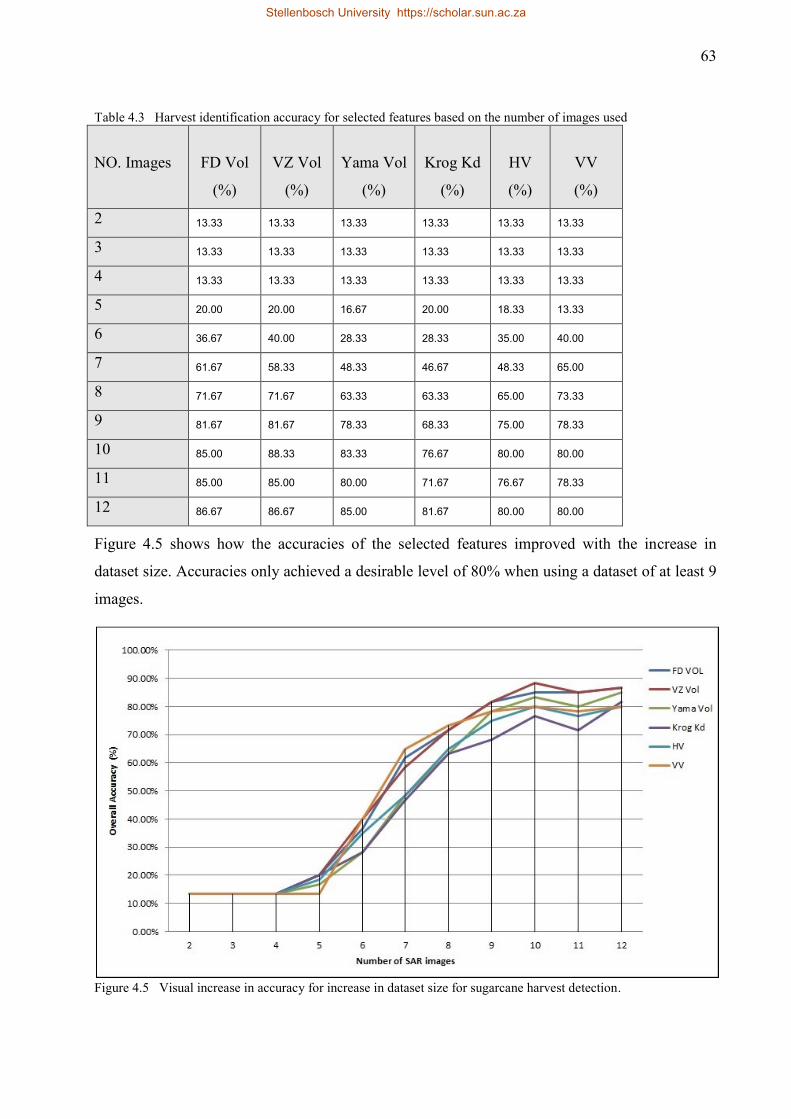
63

Table 4.3 Harvest identification accuracy for selected features based on the number of images used

NO. Images

FD Vol

(%)

VZ Vol

(%)

Yama Vol

(%)

Krog Kd

(%)

HV

(%)

VV

(%)

2 13.33 13.33 13.33 13.33 13.33 13.33

3 13.33 13.33 13.33 13.33 13.33 13.33

4 13.33 13.33 13.33 13.33 13.33 13.33

5 20.00 20.00 16.67 20.00 18.33 13.33

6 36.67 40.00 28.33 28.33 35.00 40.00

7 61.67 58.33 48.33 46.67 48.33 65.00

8 71.67 71.67 63.33 63.33 65.00 73.33

9 81.67 81.67 78.33 68.33 75.00 78.33

10 85.00 88.33 83.33 76.67 80.00 80.00

11 85.00 85.00 80.00 71.67 76.67 78.33

12 86.67 86.67 85.00 81.67 80.00 80.00

Figure 4.5 shows how the accuracies of the selected features improved with the increase in

dataset size. Accuracies only achieved a desirable level of 80% when using a dataset of at least 9

images.

Figure 4.5 Visual increase in accuracy for increase in dataset size for sugarcane harvest detection.


64

Accuracies for the Van Zyl volume scattering component peaked when using at least ten images.

The remaining five features all had improved accuracies when 12 images were used. This was

due to the nature of the technique which requires as large a dataset as possible in order to

construct statistically significant control limits. This indicates the importance of a large multi-

temporal dataset or number of samples, as identified by Panagiotidou and Nenes (2009), when

employing the proposed Shewhart individual control chart for sugarcane harvest detection.

However, a minimum of 10 images could be used in order to achieve desirable accuracies when

using the Shewhart individual control chart as a tool for harvest monitoring and identification.

4.3 Points to highlight from Experiment 1

Experiment 1 was used in order to address objective 2 of the study which was to assess multi-

temporal single feature differencing method for harvest monitoring and determine appropriate

size of RADARSAT-2 C-band dataset required for multi-temporal single feature harvest

monitoring.

The experiment achieved the following findings in relation to addressing the above objective:

1. The volume scattering features performed well in harvest monitoring, with the Freeman-

Durden volume scattering component achieving the best overall accuracy (88.33%) as

well as low errors of omission and commission of all features;

2. If a dual-polarised dataset had to be used for harvest monitoring it would be advisable to

use the cross-polarised HV backscatter channel, which achieved an overall harvest

monitoring accuracy of 80.00%;

3. When extracting feature values for each field from an image date, using the median value

does not considerably improve accuracy and, therefore, the mean value is appropriate;

4. The calculation of the MR for determining control limits for the Shewhart individual

control should be done using a simple differencing technique rather than using a ratio

value;

5. The size of the multi-temporal dataset to be used for Shewhart individual control charts

should be as large as possible in order to construct statistically significant control limits.

However, a dataset comprising ten images did provide desirable accuracies.


65

CHAPTER 5: RESULTS AND DISCUSSION EXPERIMENT 2

The objective of this experiment was to compare different machine learning classifiers, applied

to single-date, dual- and quad-polarized imagery, to determine appropriate combinations of

classifier and SAR features.

In order for the above-mentioned aim to be achieved, the following research questions were

addressed:

1. What is the effect of feature selection on classification accuracy for harvested and

unharvested sugarcane fields on a single image for both a full polarimetric and a dual

polarimetric case?

2. Which classification algorithm is best able to identify harvested and unharvested

sugarcane fields on a single image using a fully polarimetric and a dual polarimetric

dataset?

3. What is the added value of using a fully polarimetric dataset in comparison to using a

simulated dual-polarised dataset and is this added value sufficient enough to warrant the

acquisition of expensive fully polarimetric datasets when mapping sugarcane?

The overall classification accuracy and a standard deviation measure of this were used as

indication of the selected classifiers abilities to classify the harvest. This classification accuracy

was accompanied by an overall kappa statistic as well as a standard deviation of this statistic.

The classifications were performed using fully polarimetric data as well as a simulated dual

polarised scenario and a dataset containing only backscatter channels (HV and VV).

The results for feature selection (Section 5.1) for both datasets are presented, followed by the

results for classification of both datasets (Sections 5.2 and 5.3).

5.1 Feature selection

Feature selection was performed in order to reduce the dimensionality of the datasets to be used

for single image sugarcane harvest classification. Due to the range of classifiers that were tested,

it was decided that a filter be used as a feature selection technique rather than a wrapper found

embedded within selected classifiers. This decision allowed for a standardised, classifier-

independent base of feature selection prior to classification. The method used was a multi-tiered

operation whereby the Explanatory Factor Analysis (EFA) was followed by one-way Analysis of

Variance (ANOVA).


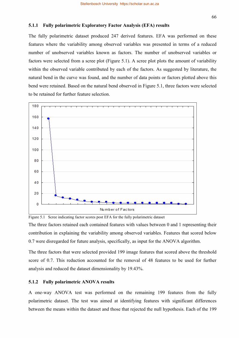
66

5.1.1 Fully polarimetric Exploratory Factor Analysis (EFA) results

The fully polarimetric dataset produced 247 derived features. EFA was performed on these

features where the variability among observed variables was presented in terms of a reduced

number of unobserved variables known as factors. The number of unobserved variables or

factors were selected from a scree plot (Figure 5.1). A scree plot plots the amount of variability

within the observed variable contributed by each of the factors. As suggested by literature, the

natural bend in the curve was found, and the number of data points or factors plotted above this

bend were retained. Based on the natural bend observed in Figure 5.1, three factors were selected

to be retained for further feature selection.

Figure 5.1 Scree indicating factor scores post EFA for the fully polarimetric dataset

The three factors retained each contained features with values between 0 and 1 representing their

contribution in explaining the variability among observed variables. Features that scored below

0.7 were disregarded for future analysis, specifically, as input for the ANOVA algorithm.

The three factors that were selected provided 199 image features that scored above the threshold

score of 0.7. This reduction accounted for the removal of 48 features to be used for further

analysis and reduced the dataset dimensionality by 19.43%.

5.1.2 Fully polarimetric ANOVA results

A one-way ANOVA test was performed on the remaining 199 features from the fully

polarimetric dataset. The test was aimed at identifying features with significant differences

between the means within the dataset and those that rejected the null hypothesis. Each of the 199


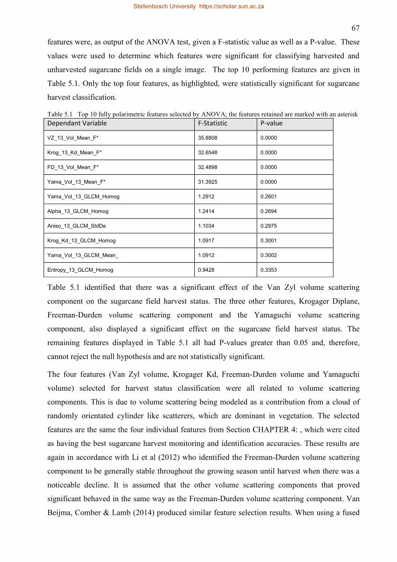
67

features were, as output of the ANOVA test, given a F-statistic value as well as a P-value. These

values were used to determine which features were significant for classifying harvested and

unharvested sugarcane fields on a single image. The top 10 performing features are given in

Table 5.1. Only the top four features, as highlighted, were statistically significant for sugarcane

harvest classification.

Table 5.1 Top 10 fully polarimetric features selected by ANOVA; the features retained are marked with an asterisk

Table 5.1 identified that there was a significant effect of the Van Zyl volume scattering

component on the sugarcane field harvest status. The three other features, Krogager Diplane,

Freeman-Durden volume scattering component and the Yamaguchi volume scattering

component, also displayed a significant effect on the sugarcane field harvest status. The

remaining features displayed in Table 5.1 all had P-values greater than 0.05 and, therefore,

cannot reject the null hypothesis and are not statistically significant.

The four features (Van Zyl volume, Krogager Kd, Freeman-Durden volume and Yamaguchi

volume) selected for harvest status classification were all related to volume scattering

components. This is due to volume scattering being modeled as a contribution from a cloud of

randomly orientated cylinder like scatterers, which are dominant in vegetation. The selected

features are the same the four individual features from Section CHAPTER 4: , which were cited

as having the best sugarcane harvest monitoring and identification accuracies. These results are

again in accordance with Li et al (2012) who identified the Freeman-Durden volume scattering

component to be generally stable throughout the growing season until harvest when there was a

noticeable decline. It is assumed that the other volume scattering components that proved

significant behaved in the same way as the Freeman-Durden volume scattering component. Van

Beijma, Comber & Lamb (2014) produced similar feature selection results. When using a fused

Dependant Variable F-Statistic P-value

VZ_13_Vol_Mean_F* 35.8808 0.0000

Krog_13_Kd_Mean_F* 32.6548 0.0000

FD_13_Vol_Mean_F* 32.4898 0.0000

Yama_Vol_13_Mean_F* 31.3925 0.0000

Yama_Vol_13_GLCM_Homog 1.2912 0.2601

Alpha_13_GLCM_Homog 1.2414 0.2694

Aniso_13_GLCM_StdDe 1.1034 0.2975

Krog_Kd_13_GLCM_Homog 1.0917 0.3001

Yama_Vol_13_GLCM_Mean_ 1.0912 0.3002

Entropy_13_GLCM_Homog 0.9428 0.3353


68

optical and SAR dataset for vegetation in salt-marsh classification, the best performing SAR

features using RF feature selection proved to be the volume scattering components. Features

relating to SAR backscatter channels did not perform well in feature selection (Van Beijma,

Comber & Lamb 2014). This is in contrast with previous research where image classification of

sugarcane, crop type and land cover using only SAR backscatter performed well (Baghdadi et al.

2009; McNairn et al. 2009; Michelson, Liljeberg & Pilesjo 2000). However, the research

conducted by Baghdadi et al. (2009), for monitoring sugarcane, used only backscatter bands for

classification. The results from the ANOVA feature selection highlight the power of added

polarimetric information in describing observed variables.

The four volume scattering features identified as statistically significant reduced the

dimensionality of the original dataset by 98.38%. These features were then used as an optimal

dataset for the single image harvest classification. The accuracy results for the classification

based on these features is presented in Section 5.2.

5.1.3 Dual polarimetric Exploratory Factor Analysis (EFA) results

The simulated dual polarimetric dataset produced 27 derived features. EFA was performed on

these features as with the fully polarimetric dataset. The number of unobserved variables or

factors was selected from a Scree plot (see Figure 5.2). The Scree plot for the dual polarised data

suggested retaining three factors for further analysis.

Number of Factors

0

1

2

3

4

5

6

7

8

9

10

11

Figure 5.2 Scree indicating factor scores post EFA for the fully polarimetric dataset


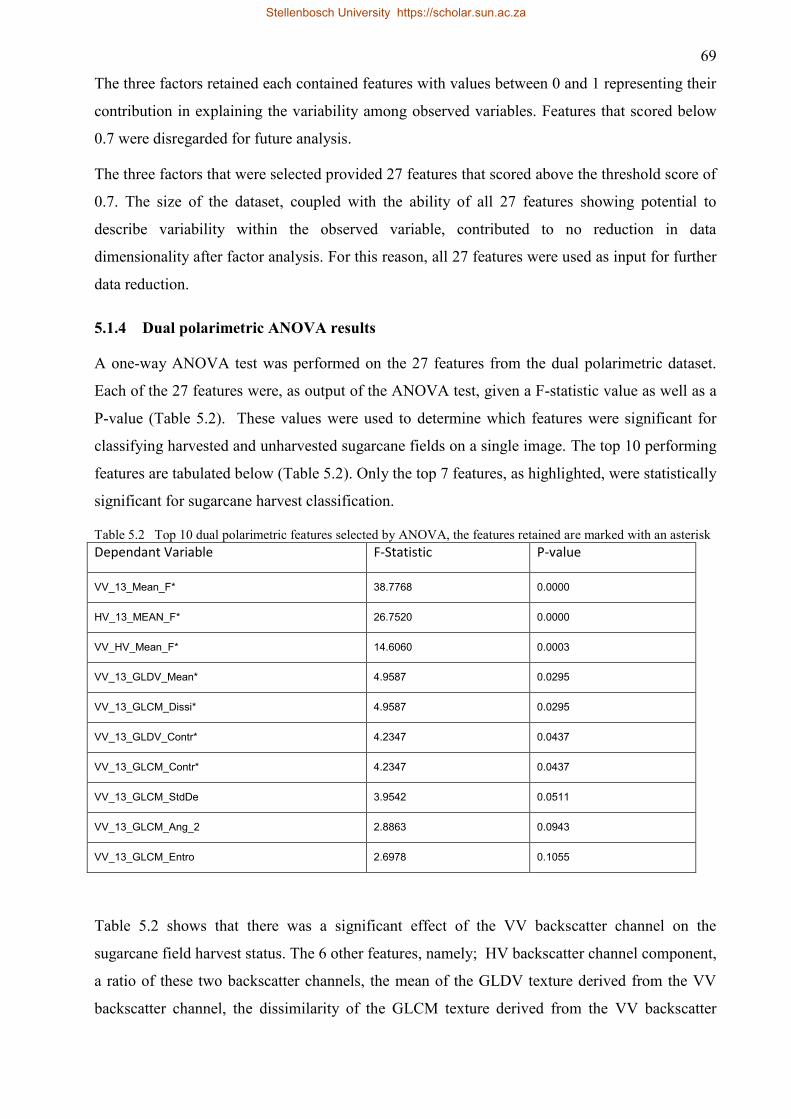
69

The three factors retained each contained features with values between 0 and 1 representing their

contribution in explaining the variability among observed variables. Features that scored below

0.7 were disregarded for future analysis.

The three factors that were selected provided 27 features that scored above the threshold score of

0.7. The size of the dataset, coupled with the ability of all 27 features showing potential to

describe variability within the observed variable, contributed to no reduction in data

dimensionality after factor analysis. For this reason, all 27 features were used as input for further

data reduction.

5.1.4 Dual polarimetric ANOVA results

A one-way ANOVA test was performed on the 27 features from the dual polarimetric dataset.

Each of the 27 features were, as output of the ANOVA test, given a F-statistic value as well as a

P-value (Table 5.2). These values were used to determine which features were significant for

classifying harvested and unharvested sugarcane fields on a single image. The top 10 performing

features are tabulated below (Table 5.2). Only the top 7 features, as highlighted, were statistically

significant for sugarcane harvest classification.

Table 5.2 Top 10 dual polarimetric features selected by ANOVA, the features retained are marked with an asterisk

Dependant Variable F-Statistic P-value

VV_13_Mean_F* 38.7768 0.0000

HV_13_MEAN_F* 26.7520 0.0000

VV_HV_Mean_F* 14.6060 0.0003

VV_13_GLDV_Mean* 4.9587 0.0295

VV_13_GLCM_Dissi* 4.9587 0.0295

VV_13_GLDV_Contr* 4.2347 0.0437

VV_13_GLCM_Contr* 4.2347 0.0437

VV_13_GLCM_StdDe 3.9542 0.0511

VV_13_GLCM_Ang_2 2.8863 0.0943

VV_13_GLCM_Entro 2.6978 0.1055

Table 5.2 shows that there was a significant effect of the VV backscatter channel on the

sugarcane field harvest status. The 6 other features, namely; HV backscatter channel component,

a ratio of these two backscatter channels, the mean of the GLDV texture derived from the VV

backscatter channel, the dissimilarity of the GLCM texture derived from the VV backscatter


70

channel, the contrast of the GLDV texture derived from the VV backscatter channel and the

contrast of the GLCM texture derived from the VV backscatter channel also displayed a

significant effect on the sugarcane field harvest status. The remaining features displayed in

Table 5.2 all had P-values greater than 0.05 and, therefore, cannot reject the null hypothesis and

are not statistically significant.

The F-statistics for the HV and VV backscatter channels, as well as the ratio between the two,

indicated high significant difference between means within the dataset, while the four texture

measures that followed showed much lower differences between means within the dataset. These

texture values still, however, proved significant based on their P-values.

The HV and VV backscatter channels displayed significant effects on sugarcane field harvest

status. This can be attributed to the potential of cross polarizations (HV) ability for vegetation

mapping, more specifically, sugarcane harvest mapping, as identified by Baghdadi et al. (2009).

It is expected that the co-polarised (VV) channel will perform well due to the interaction of co-

polarisations (VV) with the vegetation structure. Sugarcane has a long vertically orientated plant

structure which acts as dipoles, vertically polarised signals will interact strongly with them and

produce relatively high backscatter. A harvested sugarcane crop with no vertical plant structure

will result in ground return which does not return a high backscatter in the co-polarised (VV)

channels. This large variation in backscatter intensity between harvested and unharvested crops

results in the co-polarised (VV) channel being able to discriminate well between harvested and

unharvested sugarcane crops. These results are supported by the results from Section CHAPTER

4: where HV and VV backscatter channels displayed desirable accuracies when used in a single

feature harvest detection and monitoring tool. These backscatter channels have also been used

effectively for classification and monitoring in previous research using SAR data (Baghdadi et

al. 2009; McNairn et al. 2009; Michelson, Liljeberg & Pilesjo 2000).

The seven features identified as statistically significant reduced the dimensionality of the original

dataset by 74.07%. These features were then used for single image sugarcane harvest

classification. Another classification using only the 2 backscatter channels (HV and VV

backscatter) was performed in order to assess the need for further feature derivation using dual

polarimetric data. The results for this classification is presented in section 5.3.

5.1.5 Datasets for image classification

In order to clarify the results of feature dimensionality reduction (Sections 5.1.1-5.1.4), Table 5.3

presents the original dataset used as input for feature reduction, the resulting dataset at each stage


71

of feature reduction with the number of features in parenthesis and the section where the image

classification results for each dataset are presented

Table 5.3 Feature reduced datasets for image classification and the corresponding sections in the text where the

results for each are presented.

ORIGINAL DATASET CLASSIFICATION DATASET NUMBER OF FEATURES RESULTS SECTION

Fully Polarimetric

Including texture measures

All Features 247 Section 5.2.1

Post-EFA 199 Section 5.2.2

Post-ANOVA 4 Section 5.2.3

Dual Polarimetric

Including texture measures

All features 27 Section 5.3.1

Post-ANOVA 7 Section 5.3.3

Backscatter only (HV and VV) HV,VV and Ratio 3 Section 0

5.2 Fully polarimetric image classification

Classifications were performed on the SAR image number 13 (07/12/2014). Each of the six

classifiers were used for fully polarimetric image classification. Classifications were performed

at each stage of feature selection (after EFA and after ANOVA) in order to quantify the effect of

reducing dataset dimensionality.

5.2.1 Accuracy using all features

Classifications were performed on all 247 polarimetric features. Overall Accuracies (OA%) and

Kappa values were presented for each classifier in order to make comparisons. The OA% and

Kappa values are averaged as a result of 10 classifications where the training and validation data

are shuffled with each iteration. In general the tested classifiers produced high levels of

accuracy; however, the ML and the KNN classifiers performed very poorly (Table 5.4). The

highlighted results in Table 5.4 indicate the best performing classifier for each of the categories

under evaluation.

Table 5.4 Results for fully polarimetric image classification using all features

Classifier OA% STD.DEV (OA) Kappa STD.DEV (Kappa)

LIB_SVM 78.86 6.04 0.57 0.14

KNN 49.16 12.23 0.17 0.14

DT 79.21 11.43 0.56 0.24

C_SVM 81.15 2.22 0.62 0.05

RT 81.43 5.56 0.62 0.12

ML 42.31 7.54 0.04 0.21


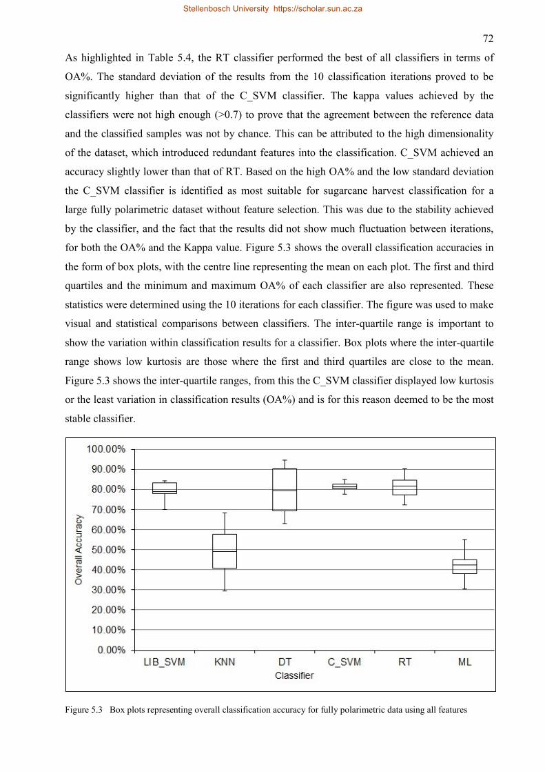
72

As highlighted in Table 5.4, the RT classifier performed the best of all classifiers in terms of

OA%. The standard deviation of the results from the 10 classification iterations proved to be

significantly higher than that of the C_SVM classifier. The kappa values achieved by the

classifiers were not high enough (>0.7) to prove that the agreement between the reference data

and the classified samples was not by chance. This can be attributed to the high dimensionality

of the dataset, which introduced redundant features into the classification. C_SVM achieved an

accuracy slightly lower than that of RT. Based on the high OA% and the low standard deviation

the C_SVM classifier is identified as most suitable for sugarcane harvest classification for a

large fully polarimetric dataset without feature selection. This was due to the stability achieved

by the classifier, and the fact that the results did not show much fluctuation between iterations,

for both the OA% and the Kappa value. Figure 5.3 shows the overall classification accuracies in

the form of box plots, with the centre line representing the mean on each plot. The first and third

quartiles and the minimum and maximum OA% of each classifier are also represented. These

statistics were determined using the 10 iterations for each classifier. The figure was used to make

visual and statistical comparisons between classifiers. The inter-quartile range is important to

show the variation within classification results for a classifier. Box plots where the inter-quartile

range shows low kurtosis are those where the first and third quartiles are close to the mean.

Figure 5.3 shows the inter-quartile ranges, from this the C_SVM classifier displayed low kurtosis

or the least variation in classification results (OA%) and is for this reason deemed to be the most

stable classifier.

Figure 5.3 Box plots representing overall classification accuracy for fully polarimetric data using all features


73

The classifiers which did not perform well, ML and KNN, had difficulty with the dimensionality

of the SAR dataset and for this reason it is likely they were not able to classify sugarcane fields

into the correct classes. These results are in contrast to those found by Myburgh and van Niekerk

(2014) who found that KNN was not significantly negatively affected by an increase in feature

dimensionality. However, the results pertaining to the ML classifier were in accordance with

Myburgh and van Niekerk (2014), who found that this classifier was unable to handle sizeable

data dimensionality.

5.2.2 Factor Analysis-reduced features

The size of the fully polarimetric dataset was then reduced, as explained in section 5.1.1, using

EFA. The reduction in the size of the dataset resulted in 199 features that were used across all

classifiers on the SAR image number 13 (07/12/2014). Overall Accuracies (OA%) and Kappa

values were presented for each classifier in order to make comparisons. The results (Table 5.5)

echoed those produced in the previous section (Section 5.2.1). In general, the tested classifiers

produced high levels of accuracy; however, the ML and the KNN classifiers performed very

poorly.

Table 5.5 Results for fully polarimetric image classification using a feature dataset reduced by EFA

Classifier OA% STD.DEV KAPPA STD.DEV

LIB_SVM 82.57 4.14 0.64 0.08

KNN 51.71 12.56 0.08 0.24

DT 82.73 7.54 0.65 0.16

C_SVM 83.31 4.37 0.66 0.09

RT 83.95 4.47 0.67 0.10

ML 54.48 10.21 0.13 0.18

Table 5.5 highlights that the RT classifier again performed the best of all classifiers in terms of

OA%; however, the standard deviation of the results from the 10 classification iterations proved

to be slightly higher than that of the LIB_SVM classifier. The reduction in dimensionality of the

dataset from the original 247 features to the 199 used here improved the classification accuracies

across all classifiers. The kappa values achieved by the classifiers, as with the original dataset,

were not high enough (>0.70) to prove that the that the agreement between the reference data and

the classified samples was not by chance. The dimensionality of the dataset, even though it was

reduced, was still large enough to possibly include redundant features into the classification. The


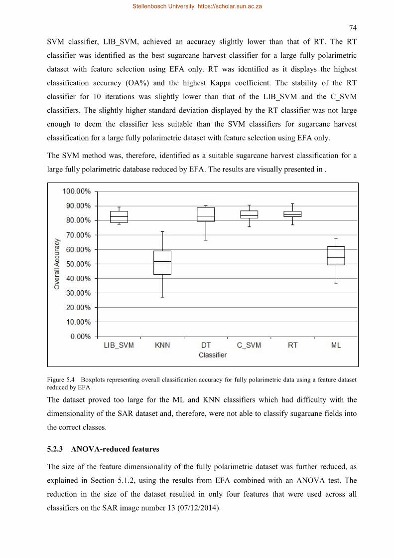
74

SVM classifier, LIB_SVM, achieved an accuracy slightly lower than that of RT. The RT

classifier was identified as the best sugarcane harvest classifier for a large fully polarimetric

dataset with feature selection using EFA only. RT was identified as it displays the highest

classification accuracy (OA%) and the highest Kappa coefficient. The stability of the RT

classifier for 10 iterations was slightly lower than that of the LIB_SVM and the C_SVM

classifiers. The slightly higher standard deviation displayed by the RT classifier was not large

enough to deem the classifier less suitable than the SVM classifiers for sugarcane harvest

classification for a large fully polarimetric dataset with feature selection using EFA only.

The SVM method was, therefore, identified as a suitable sugarcane harvest classification for a

large fully polarimetric database reduced by EFA. The results are visually presented in .

Figure 5.4 Boxplots representing overall classification accuracy for fully polarimetric data using a feature dataset

reduced by EFA

The dataset proved too large for the ML and KNN classifiers which had difficulty with the

dimensionality of the SAR dataset and, therefore, were not able to classify sugarcane fields into

the correct classes.

5.2.3 ANOVA-reduced features

The size of the feature dimensionality of the fully polarimetric dataset was further reduced, as

explained in Section 5.1.2, using the results from EFA combined with an ANOVA test. The

reduction in the size of the dataset resulted in only four features that were used across all

classifiers on the SAR image number 13 (07/12/2014).


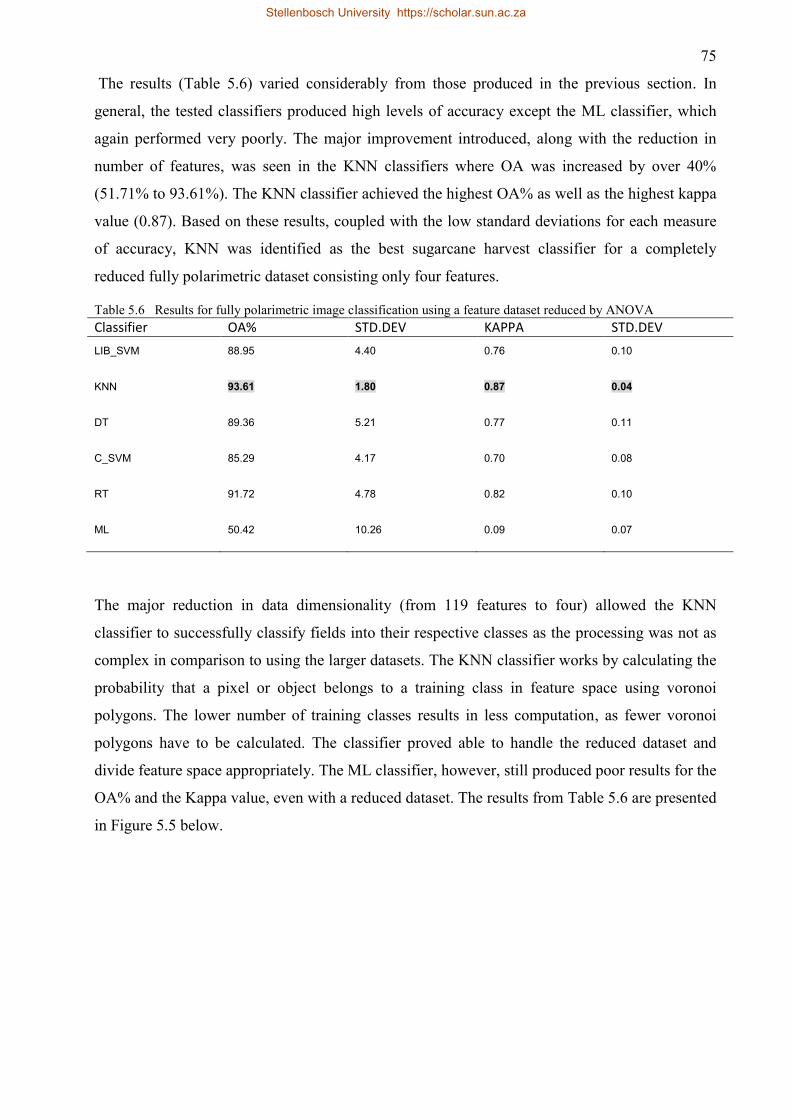
75

The results (Table 5.6) varied considerably from those produced in the previous section. In

general, the tested classifiers produced high levels of accuracy except the ML classifier, which

again performed very poorly. The major improvement introduced, along with the reduction in

number of features, was seen in the KNN classifiers where OA was increased by over 40%

(51.71% to 93.61%). The KNN classifier achieved the highest OA% as well as the highest kappa

value (0.87). Based on these results, coupled with the low standard deviations for each measure

of accuracy, KNN was identified as the best sugarcane harvest classifier for a completely

reduced fully polarimetric dataset consisting only four features.

Table 5.6 Results for fully polarimetric image classification using a feature dataset reduced by ANOVA


LIB_SVM 88.95 4.40 0.76 0.10

KNN 93.61 1.80 0.87 0.04

DT 89.36 5.21 0.77 0.11

C_SVM 85.29 4.17 0.70 0.08

RT 91.72 4.78 0.82 0.10

ML 50.42 10.26 0.09 0.07

The major reduction in data dimensionality (from 119 features to four) allowed the KNN

classifier to successfully classify fields into their respective classes as the processing was not as

complex in comparison to using the larger datasets. The KNN classifier works by calculating the

probability that a pixel or object belongs to a training class in feature space using voronoi

polygons. The lower number of training classes results in less computation, as fewer voronoi

polygons have to be calculated. The classifier proved able to handle the reduced dataset and

divide feature space appropriately. The ML classifier, however, still produced poor results for the

OA% and the Kappa value, even with a reduced dataset. The results from Table 5.6 are presented

in Figure 5.5 below.


76

Figure 5.5 Box plots representing overall classification accuracy for fully polarimetric data using a feature dataset

reduced by ANOVA

5.2.4 Fully polarimetric classification comparison

To quantify the effect of feature selection on classification and show the ability of the fully

polarimetric SAR data to classify harvested and unharvested sugarcane fields, Figure 5.6 and

Figure 5.7 are presented. Figure 5.6 shows the accuracy (OA%) achieved by each classifier at

each stage of feature selection and Figure 5.7 shows the Kappa values achieved by each

classifier at each stage of feature selection.

A general trend can be seen in Figure 5.6 which shows an increase in classification accuracy

with each stage of feature reduction. Using fewer features resulted in a general increase in

accuracy across classification algorithms except the ML classifier which decreased in accuracy

after the ANOVA stage of feature reduction. Both SVM classifiers, DT and RT, produced

desirable classification results at all stages of feature reduction. While KNN suffered under large

data dimensionality, it showed unsurpassed ability in classifying sugarcane harvest status when

four features were used. The ML classifier showed little promise for object-based image

classification when classifying sugarcane harvest. This was supported by conclusions made by

Myburgh and van Niekerk (2014) that ML’s suitability for GEOBIA was shown to be

comparatively limited when using few (<10 per class) training samples. Contrary to these results

Otukei and Blaschke (2010) found that the ML classifier for land cover classification, using an

object-based approach, was able to achieve a high overall accuracy with both large feature

dimensionality (93.91%) and reduced feature dimensionality (93.67%).


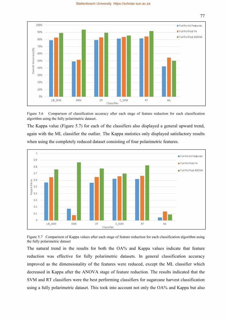
77

Figure 5.6 Comparison of classification accuracy after each stage of feature reduction for each classification

algorithm using the fully polarimetric dataset.

The Kappa value (Figure 5.7) for each of the classifiers also displayed a general upward trend,

again with the ML classifier the outlier. The Kappa statistics only displayed satisfactory results

when using the completely reduced dataset consisting of four polarimetric features.

Figure 5.7 Comparison of Kappa values after each stage of feature reduction for each classification algorithm using

the fully polarimetric dataset

The natural trend in the results for both the OA% and Kappa values indicate that feature

reduction was effective for fully polarimetric datasets. In general classification accuracy

improved as the dimensionality of the features were reduced, except the ML classifier which

decreased in Kappa after the ANOVA stage of feature reduction. The results indicated that the

SVM and RT classifiers were the best performing classifiers for sugarcane harvest classification

using a fully polarimetric dataset. This took into account not only the OA% and Kappa but also


78

the classifiers’ stability across 10 iterations. SVM has been shown to be robust under conditions

of high dimensionality (Zheng et al. 2015).

5.3 Dual polarimetric image classification

In order to mimic the first part of this experiment (Section 5.2) , classifications were performed

using a simulated dual polarimetric dataset on SAR image number 13 (07/12/2014). The dual

polarimetric dataset did not include any of the polarimetric decompositions. Each of the six

classifiers were used for image classification on simulated dual polarimetric dataset.

Classifications were performed at each stage of feature selection on the simulated dual

polarimetrc dataset as well as using only the HV and VV backscatter channels; this allowed for

drawing conclusions relating to what SAR features are useful for sugarcane harvest mapping,

whether fully polarimetric data is necessary for sugarcane harvest mapping and processing

requirements.

5.3.1 Dual polarimetric classification using all features

Classifications for all six classifiers were performed using all features derived from the dual

polarimetric dataset; 27 features were used in classification. Overall accuracies achieved by the

classifiers were much lower than that of the fully polarimetric dataset at this stage of feature

reduction (Table 5.7). The DT and RT classifiers produced the highest levels of OA%, 87.23%

and 88.95%, respectively. The kappa values of these classifiers indicated that the agreement

between the reference data and the classified samples was not by chance. The C_SVM classifier

achieved an accuracy of 74.25%; however, the kappa value (0.45) indicated that the classifier

was not suitable for single date sugarcane harvest classification. The standard deviation measures

accompanying each of the accuracy validation statistics were used to express the stability of the

classifier across 10 iterations.

Table 5.7 Results for dual polarimetric image classification using all features


LIB_SVM 68.11 7.14 0.33 0.14

KNN 43.43 12.17 -0.15 0.23

DT 87.23 5.93 0.74 0.12

C_SVM 74.25 8.11 0.45 0.17

RT 88.95 6.05 0.77 0.13

ML 51.98 11.84 -0.04 0.22


79

The accuracy (OA%) of the dual polarimetric dataset (Table 5.7) was generally lower than that

of the fully polarimetric dataset when all features were used. This can be attributed to the number

and nature of the features. There are fewer dual polarimetric features and they do not possess the

same predictive power displayed by the fully polarimetric dataset. For this reason, in general, the

classifiers had difficulty in separating the harvested from unharvested fields in feature space. The

box plots in Figure 5.8 depict the overall classification accuracies, represented by a line

representing the mean on each box plot, the first and third quartiles and the minimum and

maximum OA% of each classifier. These statistics were determined using the 10 iterations for

each classifier. The figure was used to make visual comparisons between classifiers with the

most stable classifier (DT) displaying the lowest inter-quartile range and low kurtosis of the

quartiles around the mean.

Figure 5.8 Box plots representing overall classification accuracy for dual polarimetric data using all features

When using all features derived from dual polarimetric SAR data, again, the ML and KNN

classifiers displayed a lack in ability to classify the dataset. As with the fully polarimetric

dataset, this provided contrast with the results found by Myburgh and van Niekerk (2014) who

found that KNN was not significantly negatively affected by an increase in feature

dimensionality. However, the results pertaining to the ML classifier were in accordance with

Myburgh and van Niekerk (2014), who found that the classifier was unable to handle sizeable

data dimensionality. Pal and Mather (2006) found contrasting results to those of this study and

that of Myburgh and van Niekerk (2014). The ML classifier for land cover classification using


80

Landsat-7 increased in accuracy with an increase in number of features (Pal & Mather 2006).

This was supported by Otukei and Blaschke (2010) who found the ML classifier was able to

achieve a high overall accuracy with both large feature dimensionality (93.91%) and reduced

feature dimensionality (93.67%).

The DT classifier proved to be the most stable for sugarcane harvest classification; however, the

RT classifier achieved the highest classification results using all features derived from a dual

polarimetric dataset, and the measure of stability was negligible in comparison with the DT

classifier. This leads to the conclusion that the best sugarcane harvest classifier for a large dual

polarimetric dataset without feature selection was the RT classifier.

5.3.2 Dual polarimetric classification post EFA

The factor analysis stage of feature reduction did not achieve any reduction in the data

dimensionality and for this reason the classification results were the same as in section 5.3.1

prior to this where all features derived from the dual polarimetric dataset were used.

5.3.3 Dual polarimetric classification post ANOVA

The feature dimensionality of the dual polarimetric dataset was reduced, as explained in Section

5.1.4, using the results from the ANOVA test. The reduction in the size of the dataset resulted in

only seven features that were used across all classifiers on the SAR image number 13

(07/12/2014).

Table 5.8 presents the classification results achieved using the seven features. The OA%

achieved by the classifiers was lower compared to the use of all features derived from the dual

polarimetric dataset. Only the DT classifier achieved accuracies above 80% for classification of

the sugarcane harvest status. However, the kappa value for this classifier indicated that the use of

the classification model was not ideal. The OA% of the RT classifier was lower than when all

dual polarimetric features were used, and the high standard deviation of the OA% across 10

iterations indicates the classifier was not consistent in achieving the 76.45% accuracy depicted in

Table 5.8.


81

Table 5.8 Results for dual polarimetric image classification using a feature dataset reduced by ANOVA


LIB_SVM 74.89 8.73 0.51 0.16

KNN 40.99 8.05 -0.15 0.21

DT 80.85 9.08 0.62 0.17

C_SVM 77.48 6.34 0.55 0.13

RT 76.47 12.05 0.53 0.24

ML 70.88 10.74 0.41 0.21

A box plot of the results in Table 5.8 is presented below in Figure 5.9 . The box plots indicate

that across all classification methods, the accuracies achieved were not stable as the distribution

of the quartiles around the mean show high kurtosis and include outliers.

Figure 5.9 Box plots representing overall classification accuracy for dual polarimetric data using a feature dataset

reduced by ANOVA

The poor results achieved using a reduced dataset can be explained by the poor predictive power

of texture measures derived from SAR. Four of the seven selected features were of texture nature

and, therefore, caused confusion for the classifiers. It is in contrast with Li et al. (2012) and

Herold, Haack and Solomon (2004) who found that adding even one texture measure to L- and

C-band data provided a better classification.


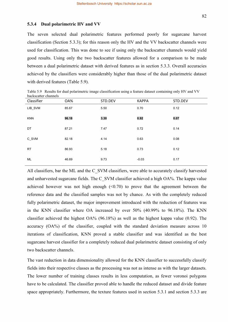
82

5.3.4 Dual polarimetric HV and VV

The seven selected dual polarimetric features performed poorly for sugarcane harvest

classification (Section 5.3.3); for this reason only the HV and the VV backscatter channels were

used for classification. This was done to see if using only the backscatter channels would yield

good results. Using only the two backscatter features allowed for a comparison to be made

between a dual polarimetric dataset with derived features as in section 5.3.3. Overall accuracies

achieved by the classifiers were considerably higher than those of the dual polarimetric dataset

with derived features (Table 5.9).

Table 5.9 Results for dual polarimetric image classification using a feature dataset containing only HV and VV

backscatter channels


LIB_SVM 85.67 5.50 0.70 0.12

KNN 96.18 3.30 0.92 0.07

DT 87.21 7.47 0.72 0.14

C_SVM 82.18 4.14 0.63 0.08

RT 86.93 5.18 0.73 0.12

ML 46.69 9.73 -0.03 0.17

All classifiers, bar the ML and the C_SVM classifiers, were able to accurately classify harvested

and unharvested sugarcane fields. The C_SVM classifier achieved a high OA%. The kappa value

achieved however was not high enough (<0.70) to prove that the agreement between the

reference data and the classified samples was not by chance. As with the completely reduced

fully polarimetric dataset, the major improvement introduced with the reduction of features was

in the KNN classifier where OA increased by over 50% (40.99% to 96.18%). The KNN

classifier achieved the highest OA% (96.18%) as well as the highest kappa value (0.92). The

accuracy (OA%) of the classifier, coupled with the standard deviation measure across 10

iterations of classification, KNN proved a stable classifier and was identified as the best

sugarcane harvest classifier for a completely reduced dual polarimetric dataset consisting of only

two backscatter channels.

The vast reduction in data dimensionality allowed for the KNN classifier to successfully classify

fields into their respective classes as the processing was not as intense as with the larger datasets.

The lower number of training classes results in less computation, as fewer voronoi polygons

have to be calculated. The classifier proved able to handle the reduced dataset and divide feature

space appropriately. Furthermore, the texture features used in section 5.3.1 and section 5.3.3 are


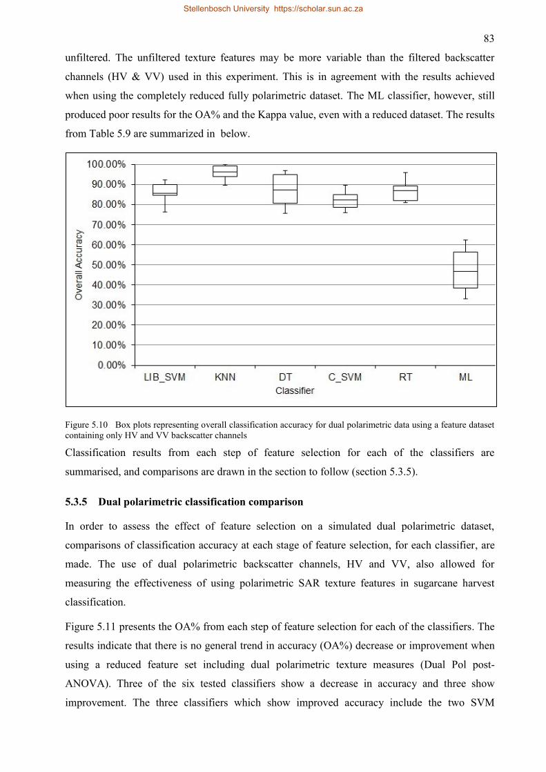
83

unfiltered. The unfiltered texture features may be more variable than the filtered backscatter

channels (HV & VV) used in this experiment. This is in agreement with the results achieved

when using the completely reduced fully polarimetric dataset. The ML classifier, however, still

produced poor results for the OA% and the Kappa value, even with a reduced dataset. The results

from Table 5.9 are summarized in below.

Figure 5.10 Box plots representing overall classification accuracy for dual polarimetric data using a feature dataset

containing only HV and VV backscatter channels

Classification results from each step of feature selection for each of the classifiers are

summarised, and comparisons are drawn in the section to follow (section 5.3.5).

5.3.5 Dual polarimetric classification comparison

In order to assess the effect of feature selection on a simulated dual polarimetric dataset,

comparisons of classification accuracy at each stage of feature selection, for each classifier, are

made. The use of dual polarimetric backscatter channels, HV and VV, also allowed for

measuring the effectiveness of using polarimetric SAR texture features in sugarcane harvest

classification.

Figure 5.11 presents the OA% from each step of feature selection for each of the classifiers. The

results indicate that there is no general trend in accuracy (OA%) decrease or improvement when

using a reduced feature set including dual polarimetric texture measures (Dual Pol post-

ANOVA). Three of the six tested classifiers show a decrease in accuracy and three show

improvement. The three classifiers which show improved accuracy include the two SVM


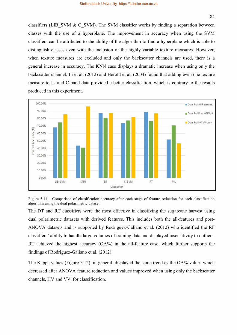
84

classifiers (LIB_SVM & C_SVM). The SVM classifier works by finding a separation between

classes with the use of a hyperplane. The improvement in accuracy when using the SVM

classifiers can be attributed to the ability of the algorithm to find a hyperplane which is able to

distinguish classes even with the inclusion of the highly variable texture measures. However,

when texture measures are excluded and only the backscatter channels are used, there is a

general increase in accuracy. The KNN case displays a dramatic increase when using only the

backscatter channel. Li et al. (2012) and Herold et al. (2004) found that adding even one texture

measure to L- and C-band data provided a better classification, which is contrary to the results

produced in this experiment.

Figure 5.11 Comparison of classification accuracy after each stage of feature reduction for each classification

algorithm using the dual polarimetric dataset.

The DT and RT classifiers were the most effective in classifying the sugarcane harvest using

dual polarimetric datasets with derived features. This includes both the all-features and post-

ANOVA datasets and is supported by Rodriguez-Galiano et al. (2012) who identified the RF

classifiers’ ability to handle large volumes of training data and displayed insensitivity to outliers.

RT achieved the highest accuracy (OA%) in the all-feature case, which further supports the

findings of Rodriguez-Galiano et al. (2012).

The Kappa values (Figure 5.12), in general, displayed the same trend as the OA% values which

decreased after ANOVA feature reduction and values improved when using only the backscatter

channels, HV and VV, for classification.


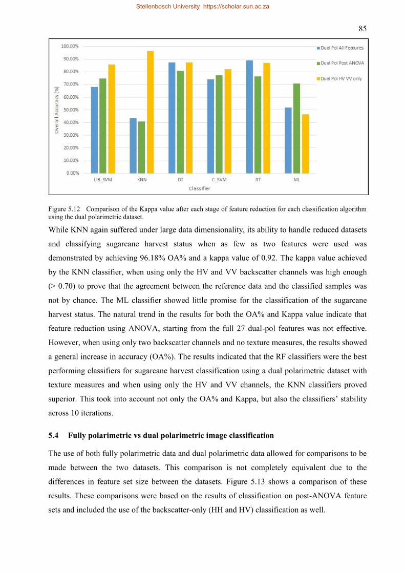
85

Figure 5.12 Comparison of the Kappa value after each stage of feature reduction for each classification algorithm

using the dual polarimetric dataset.

While KNN again suffered under large data dimensionality, its ability to handle reduced datasets

and classifying sugarcane harvest status when as few as two features were used was

demonstrated by achieving 96.18% OA% and a kappa value of 0.92. The kappa value achieved

by the KNN classifier, when using only the HV and VV backscatter channels was high enough

(> 0.70) to prove that the agreement between the reference data and the classified samples was

not by chance. The ML classifier showed little promise for the classification of the sugarcane

harvest status. The natural trend in the results for both the OA% and Kappa value indicate that

feature reduction using ANOVA, starting from the full 27 dual-pol features was not effective.

However, when using only two backscatter channels and no texture measures, the results showed

a general increase in accuracy (OA%). The results indicated that the RF classifiers were the best

performing classifiers for sugarcane harvest classification using a dual polarimetric dataset with

texture measures and when using only the HV and VV channels, the KNN classifiers proved

superior. This took into account not only the OA% and Kappa, but also the classifiers’ stability

across 10 iterations.

5.4 Fully polarimetric vs dual polarimetric image classification

The use of both fully polarimetric data and dual polarimetric data allowed for comparisons to be

made between the two datasets. This comparison is not completely equivalent due to the

differences in feature set size between the datasets. Figure 5.13 shows a comparison of these

results. These comparisons were based on the results of classification on post-ANOVA feature

sets and included the use of the backscatter-only (HH and HV) classification as well.


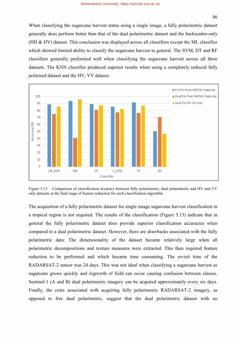
86

When classifying the sugarcane harvest status using a single image, a fully polarimetric dataset

generally does perform better than that of the dual polarimetric dataset and the backscatter-only

(HH & HV) dataset. This conclusion was displayed across all classifiers except the ML classifier

which showed limited ability to classify the sugarcane harvest in general. The SVM, DT and RF

classifiers generally performed well when classifying the sugarcane harvest across all three

datasets. The KNN classifier produced superior results when using a completely reduced fully

polarised dataset and the HV, VV dataset.

Figure 5.13 Comparison of classification accuracy between fully polarimetric, dual polarimetric and HV and VV

only datasets at the final stage of feature reduction for each classification algorithm

The acquisition of a fully polarimetric dataset for single image sugarcane harvest classification in

a tropical region is not required. The results of the classification (Figure 5.13) indicate that in

general the fully polarimetric dataset does provide superior classification accuracies when

compared to a dual polarimetric dataset. However, there are drawbacks associated with the fully

polarimetric data: The dimensionality of the dataset became relatively large when all

polarimetric decompositions and texture measures were extracted. This then required feature

reduction to be performed and which became time consuming. The revisit time of the

RADARSAT-2 sensor was 24 days. This was not ideal when classifying a sugarcane harvest as

sugarcane grows quickly and regrowth of field can occur causing confusion between classes.

Sentinel-1 (A and B) dual polarimetric imagery can be acquired approximately every six days.

Finally, the costs associated with acquiring fully polarimetric RADARSAT-2 imagery, as

opposed to free dual polarimetric, suggest that the dual polarimetric dataset with no


87

decompositions and texture measures be used for single image sugarcane harvest classification in

a tropical region.

Conclusions drawn from the comparison of the datasets are highlighted in the section to follow.

5.5 Points to highlight from Experiment 2

Experiment 2 was used in order to address Objective 3 of the study which was to assess

RADARSAT-2 C-band individual image sugarcane harvest classification methods, for both

fully-polarimetric and simulated dual polarimetric datasets, and determine the effectiveness of

obtaining and implementing a fully polarimetric dataset as opposed to a dual polarimetric dataset

for individual image harvest classification.

The experiment achieved the following findings in relation to addressing the above objective:

1. The chosen method of feature selection proved to be successful for the fully polarimetric

dataset, improving accuracy of all classifiers considerably. When using a dual polarimetric

dataset, the reduction in feature dimensionality did not show a trend in lowering or

improving the OA% of the classifiers. This can be related to the use of SAR texture

measures in the dual polarimetric dataset, which became apparent when superior results

were achieved using only the HV and the VV backscatter channels for classification.

2. When using a dataset with severly reduced dimensionality (< four) to classify harvested

and unharvested sugarcane fields, it is suggested that the KNN with a K value of 1 is used

for both the fully polarimetric and dual polarimetric datasets.

3. When classifying the sugarcane harvest status on a single SAR image, HV and VV

backscatter channels produced results superior to that of the fully polarimetric dataset. For

operational use, it is preferable to use dual polarimetric backscatter channels only as it

requires less monetary resources and fewer processing requirements.

In Chapter 6, results from Experiments 1 and 2 will be summarised and conclusions are drawn

from the results. The results will also be put into context in terms of existing research and

knowledge they have contributed. Recommendations relating to research stemming from the

study, as well as recommendations for operational use of the results, are also made.


88

CHAPTER 6: CONCLUSION

Experiments 1 and 2 which were designed to address the objectives set out for the research. The

experiments aimed to identify a single SAR polarimetric feature for sugarcane harvest

monitoring and detection, as well as assess the accuracy of selected object based image

classification methods for single image sugarcane harvest classification. The sections ahead

summarise the findings of the study and how they compare with previous studies. The

contributions the study has made to the fields of polarimetric SAR and harvest monitoring as

well as the limitations associated with the study are also presented. Recommendations, both for

operational use and for further research are then suggested, followed by concluding remarks

about the study and the direction for the continuation of the research.

6.1 SYNTHESIS AND FINDINGS OF THE STUDY

The following sections present a summary of the findings from the experiments performed in

order to achieve the aim of the study and address the research questions proposed.

6.1.1 Experiment 1

The aim of Objective 2 was to assess a multi-temporal single feature differencing method for

harvest monitoring and determine the appropriate size of a RADARSAT-2 C-band dataset

required for multi-temporal single feature harvest monitoring. This was assessed and achieved by

Experiment 1, which made use of Shewhart individual control charts. The Shewhart control

charts were used to assess both the accuracy of harvest identification for individual polarimetric

SAR features.

When assessing the ability of single polarimetric features to identify the sugarcane harvest, the

volume scattering components from each of the polarimetric decompositions consistently

outperformed other SAR features in its ability to detect harvest. The backscatter channels, HV

and VV, also proved effective in identifying the sugarcane harvest. Anisotropy, Alpha, Entropy,

odd bounce features and double bounce features proved to have limited ability in identifying the

sugarcane harvest. These features also ranked highly in the features selected from fully

polarimetric feature selection in Experiment 2.

The second part of this experiment assessed each of these four volume scattering components as

well as the HV and VV backscatter channels as single features for harvest monitoring. The

ability of a feature to monitor the sugarcane harvest efficiently was assessed using errors of

commission and omission. As expected, all features performed well, and the Freeman-Durden

volume scattering component was the best performing feature with an overall accuracy of


89

88.33%, a kappa value of 0.749, an average error of commission of 8.23% and average error of

omission of 15.02%. In the theoretical case where only dual polarimetric data was available, the

HV backscatter channel would be the appropriate feature for sugarcane harvest monitoring with

an overall accuracy of 80.00%, a kappa value of 0.724, an average error of commission of 8.23%

and average error of omission of 11.85%. This was also true for dual polarimetric feature

selection in Experiment 2, where HV was selected as a feature which contributed most in

explaining the sugarcane harvest status. The effect of ratioing versus difference and mean versus

median for calculation of moving range was also tested.. When calculating moving range, it was

found that using a differencing technique from one date to the next is advisable since using a

ratio does not improve accuracy. The use of mean values for data analysis was also found to be

sufficient as the use of median values does not provide improved accuracy and therefore the

extra processing is not warranted.

The Shewhart individual control charts are multi-temporal in nature and, therefore, requires a

time series of datasets. The minimum size of the dataset in order to achieve desirable accuracies

(>80%) and construct statistically significant control limits for sugarcane harvest detection and

monitoring was found to be 9 images. However, it is advisable to use the largest amount of

image dates available.

The results and findings drawn from these answered Objective 2 and the research questions

derived from the objective.

6.1.2 Experiment 2

Experiment 2 was designed in order to address and achieve Objective 3 of the study, which was

to assess RADARSAT-2 C-band individual image sugarcane harvest classification methods, for

both fully-polarimetric and simulated dual polarimetric datasets, and determine the effectiveness

of obtaining and implementing a fully polarimetric dataset, as opposed to a dual polarimetric

dataset for individual image harvest classification.

Feature selection was done in two steps, EFA followed by ANOVA. The two-tiered feature

selection proved to be successful for the fully polarimetric dataset, reducing the dataset to only

four features and improving the accuracy of all classifiers (with the exception of ML)

considerably at all stages of feature reduction. The four features selected were all volume

scattering components of the polarimetric decompositions and did not feature any texture or

backscatter measures. This highlights that the derivation of textures using SAR features did not

assist in classifying the sugarcane harvest. The selection of the volume scattering components


90

agrees with the results achieved in Experiment 1 where volume scattering components achieved

superior results.

When using a dual polarimetric dataset, however, the reduction in feature dimensionality

lowered the OA% of some of the classifiers. The feature reduction method reduced the dataset to

7 features; this included the selection of the HV, VV backscatter channels and a ratio of these

backscatter channels. The decrease in classification accuracy can be related to the SAR texture

measures which contain more variability as they are not filtered.This became apparent when

superior results were achieved using only the HV and the VV backscatter channels for

classification.

When classifying the sugarcane harvest status on a single SAR image, HV and VV backscatter

channels produced results superior to those of the fully polarimetric dataset. For operational use,

it is advised to use dual polarimetric backscatter channels only as these require less monetary

resources and fewer processing requirements.

When using a dataset with reduced dimensionality to classify harvested and unharvested

sugarcane fields, it is suggested that the KNN with a K value of 1 is used for both fully

polarimetric and dual polarimetric datasets. This classifier was able to handle the small

dimensionality of the reduced datasets and achieved exceptional results for sugarcane harvest

classification on a single image. These results were replicated across the fully polarimetric

dataset and the dual polarimetric dataset.

The results and findings drawn from these answered Objective 3 and the research questions

derived from the objective.

6.2 CONTEXTUALIZING THE FINDINGS

Very little research has been done into using SAR, both fully polarimetric and dual polarimetric

for sugarcane harvest monitoring. Harvest monitoring in itself has not been investigated

extensively. This led to multi-temporal crop monitoring has been at the heart of research

pertaining to crop change detection. Much of this research has focused on the monitoring of rice

crops and for this reason comparisons made with literature need to take into account differences

between plant structure between the various crops and are not always relevant when referring to

sugarcane.

The results from this study, when using fully polarimetric data and decompositions for harvest

monitoring and classification, show a strong relationship between the volume scattering

components for explaining crop status. In agreement with these results, Turkar and Rao (2011)

found that the Van Zyl volume scattering component resulted in the highest crop type


91

classification accuracy. As with this study, they also found that when using all decomposition

features, the Van Zyl and Freeman-Durden volume scattering contributed significantly to overall

accuracy. This was further supported by Wang et al. (2013) who identified the Freeman-Durden

decomposition as one that provides a better understanding of the physical scattering mechanisms

without additional terrain information. Van Beijma, Comber and Lamb (2014), when using a

fused optical and SAR dataset, identified the best performing SAR features proved to be the

volume scattering components. Hoesseini et al. (2011) found the highest classification accuracy

for land cover classification achieved was using the Krogager decomposition. In contrast to this

result, Jiao et al. (2014), using multi-temporal Radarasat-2 C-band data, found that Cloude–

Pottier decomposition parameters provided the best classification accuracy the Freeman–Durden

decomposition. This was in stark contrast to the results produced in this study, where Cloude-

Pottier parameters were not influential.

In the case of using a dual polarimetric dataset, the harvesting monitoring tool suggested in this

thesis as well as the sugarcane harvest classification results, produced the most effective results

when using the cross polarised HV backscatter channel, while the VV backscatter channel

proved to show similar potential for these applications. The success of these features were

verified by literature - Jiao et al. (2014) stated there was a strong relationship between the

phenological growth stage and HV backscatter channels for canola crops; Deschamps et al.

(2012) identified that the HV and VV polarizations had the most significant contributions for

radar-only clop classifications with the HH backscatter having very little contribution. Inoue et

al. (2014) found that the backscatter coefficient for C-band HV channel is strongly correlated

with the amount and structure of leaf elements within a canopy. These backscatter channels have

also been used effectively for classification and monitoring in previous research using SAR data

(McNairn et al. 2009; Michelson, Liljeberg & Pilesjo 2000). However, Lopez-Sanchez, Cloude

and Ballester-Berman (2012) cited that the HH and VV backscatter channels showed a temporal

variation that has a significant correlation with the development of the rice plants during the

growth season.

The use of texture measures for classification in this study showed that texture derived from

SAR data does not improve accuracy; when texture measures are excluded and only the

backscatter channels are used, there is a dramatic increase in accuracy. Li et al. (2012) and

Herold et al. (2004) found that adding even one texture measure to L- and C-band data provided

a better classification, and this is in contrast of the results produced in this experiment.

In the context of sugarcane and SAR, very few studies have been conducted and for this reason

comparisons with literature are few. In accordance with results achieved in this study, Baghdadi


92

et al. (2009) found the HV and VV backscatter channels displayed significant effects on

sugarcane field harvest status. This can be attributed to the multiple scattering and depolarisation

of the signal in a volume of vegetation, more specifically, sugarcane. Sugarcane has a long

vertically orientated plant structure which acts as dipoles, vertically polarised signals will

interact strongly with them and produce relatively high backscatter. A harvested sugarcane crop

with no vertical plant structure will result in ground return which does not return a high

backscatter in the co-polarised (VV) channels.

Although it is advised to use a dataset of low complexity, when using a high dimensional dataset,

the SVM classifier was the best performing algorithm for SAR data. The RT classifier achieved

the best OA% result however the C_SVM classifier displayed low kurtosis or the least variation

in classification results (OA%) and is for this reason deemed to be the most stable classifier. This

is in line with Hosseini et al. (2011) who indicate that the SVM classifier can be used as an

effective method for fully polarimetric SAR images with acceptable levels of accuracy.

Similarly, Oomen et al. (2008), Zheng et al. (2015) and Adam et al. (2014) found that the SVM

classifier was effective when dealing with large datasets, not only SAR-based datasets. When

using the optimally reduced datasets, the results pertaining to the KNN classifier were not in

accordance with Myburgh and van Niekerk (2014) who found that KNN was not significantly

negatively affected by an increase in feature dimensionality. However, the results achieved by

the KNN in this study using a large dataset suggest otherwise. The KNN did achieve the best

classification accuracy when using the optimally reduced datasets for both fully polarimetric and

dual polarimetric data. These conclusions diverge from Fontenelli et al. (2015) who found the

best results for rice crops classification using SAR C-band data were achieved using DT

classifiers.

6.3 CONTRIBUTION AND NOVELTY

The completion of the study allowed for the synthesis of the results and conclusions to be drawn

from this.

It was shown that Shewhart individual control charts show potential for sugarcane harvest

monitoring using polarimetric SAR. The method allows a statistical confidence to be placed on

harvest monitoring. Harvest monitoring using RS features has previously not adapted this

statistical confidence to harvest identification and monitoring. While the added phase

information present in fully polarimetric data does improve accuracy this data is not always

available, and the dual polarimetric features achieved accuracies acceptable for operational use,

as demonstrated in Experiment 1. When implementing the Shewhart individual control charts for

harvest monitoring, it is advised to use the largest dataset available to the user.


93

When classifying the sugarcane harvest using datasets of large dimensionality, specifically the

fully polarimetric dataset with derived polarimetric decompositions and textures, the SVM

classifier handles these large datasets producing desirable accuracies. Using as few features as

possible, following a data reduction method is advised. The simple dimensionality of the dataset

allows for the use of a computationally simple classifier, KNN with a K value of 1, and improves

classification accuracies for both the fully polarimetric and dual polarimetric datasets. The

addition of texture measures derived from both the fully polarimetric datasets and the dual

polarimetric datasets does not improve accuracy for SAR harvest classification. The omission of

these texture features in classification will improve computational time and place less strain on

image processing resources.

The accuracies achieved for both experiments, by using only the HV and VV backscatter

channels, suggest the potential of dual polarimetric sensors for harvest monitoring and

classification, posing many research and operational prospects as Sentinel-1 data is now freely

available. This study has provided insight into methods that can be used for harvest monitoring

and classification by identifying features that are suitable these applications and, in that, aided in

understanding data pre-processing and preparation of complex SAR datasets.

6.4 LIMITATIONS

Limitations within the study mainly stemmed from the complexity of the ground truth and

training database. The training database provided data for an initial 854 sugarcane fields

monitored by CIRAD. The method used for acquiring the validation data proved to be

problematic as the data collection did not coincide with the actual harvest date for most of the

methods used. Individuals working in the field to record harvest status did not always have

accurate measurements of when the harvest occurred and the recording of the harvest status with

the use of SPOT images, whose acquisition date did not coincide with the RADARSAT-2 image

date, resulted in data acquired with these acquisition methods to be discarded. Due to the rapid

regrowth of sugarcane following a harvest, the date of recording of harvest information needs to

coincide with the date of the actual harvest. The quality of the reference resulted in only 65 fields

available for analysis, resulting in the spread of harvested and unharvested fields per image date

to be highly skewed. Therefore, classifiers were only trained using a late season image, for the

purpose of effectively training a classifier images from earlier in the season where not used. The

number of fields (65) was also a limitation as the sample was small and did not represent the true

population of sugarcane fields.

Another limitation within the study was due to the design of the classification scheme. Due to

the fact that only harvested and unharvested fields were classified, again, ground truth data


94

pertaining to partially harvested fields had to be discarded. This was influenced by the study area

as heterogeneity of harvest status within fields at any one point is common as automation of the

harvest is not widely available due to the steep landscapes, and manual harvests can last number

of weeks. The conclusions drawn from the study are limited to the case of sugarcane on Rèunion

Island for one image date and therefore cannot be accepted as universally true for all sugarcane

areas.

6.5 RECOMMENDATIONS

The results achieved using Experiments 1 and 2 for addressing the aim of the study have allowed

for recommendations to be suggested for sugarcane harvest monitoring. These are summarised in

the sections to follow which present operational recommendations based on the results as well as

further research questions stemming from experiments 1 and 2. Operational and research

recommendations are presented separately as the study was conducted for research purposes

however the collaboration with CIRAD required that operational recommendations do stem from

the study.

6.5.1 Operational recommendations

The study yielded findings that can be useful for an operational sugarcane harvest monitoring

system.

The Shewhart individual control charts have never been applied as a tool for harvest monitoring,

Experiment 1 demonstrated the promising ability for this method to be used in harvest

monitoring. In countries or regions such as Rèunion island where sugarcane mills are only

operational if a sufficient amount of sugarcane is available for milling, developing a cost-

efficient, easily accessible sugarcane monitoring application is extremely important. Factories

can predict the amount of sugarcane that has been harvested and, therefore, calculate how much

harvested sugarcane they can still expect and effectively plan for mill operation time, thus

greatly reducing costs and improving yields. This tool also allows for the development of

sugarcane harvest archives, in turn allowing for improvement in the agriculture industry,

especially in countries where sugarcane is a dominant crop. Experiment 1 demonstrated the need

for a large dataset in order to improve results, and the sugarcane mills have appropriate resources

to acquire a database of images needed for this harvest monitoring tool.

In order to reduce costs associated with acquisition of fully polarimetric data it is recommended

that a dual polarimetric dataset be acquired for operational use in sugarcane harvest monitoring

on Rèunion Island. Dual polarimetric datasets are often more affordable and even free of cost in

some instances (Sentinel-1). The performance when using only the HV and VV backscatter


95

bands indicates that the use of Sentinel-1 data (VH-VV) for sugarcane harvest classification is

possible at a high accuracy (>80%) when using a KNN classifier.

The use of a single image for harvest status classification will reduce costs associated with data

acquisition and will, therefore, be more easily accessible to these small-scale farmers. Large

operational sugarcane mills can also use single image harvest classification to make comparisons

with the amount of received sugarcane and the amount harvested, again optimising milling

processes and reducing costs applicable to the mills.

This research has not yet developed the optimal tool for harvest monitoring and classification;

however, the initial processing steps towards an operational tool for harvest monitoring were

investigated, assessed and achieved. In order to optimise these tools for operational

implementation, further investigation into effective sugarcane harvest monitoring needs to be

addressed.

6.5.2 Research recommendations

In order to optimise the tools for harvest monitoring and identification, further investigation

beyond the scope of this study needs to be done.

Firstly, an accurate ground truth database with a larger selection of training and verification data

is required. This study was performed using relatively small fields, and it is suggested to expand

the database to larger sugarcane fields not only operated by small-scale farmers.

Future research should aim to replicate the classification methods tested in this study and

introduce a third class, partially harvested, into the classification schema. This will allow for a

more realistic harvest monitoring and identification tool. The classification schema used only

included harvested and unharvested classes. This is not optimal as sugarcane fields are often

heterogeneous due to the large acreages associated with sugarcane fields as well as the manual

harvesting of these fields, and are, for this reason, often partially harvested at the time of image

acquisition. It is also recommended that future research test the transferability of the

classification methodology. The classification methodology was also only tested on one image

date. In order to accurately validate the harvest classification method, images from different

periods in the growing season need to be incorporated into the analysis.

The classification methods used were also used on the default classification parameters, as

proposed by the SLICE software. While accuracies achieved were desirable, it is suggested that

the parameters of certain classifiers be assessed in order to possibly improve the accuracies, in

turn creating for a more optimised harvest monitoring and classification method. For operational


96

use, it is required that all parameters be defined within the harvest monitoring tool and, thus, if

the optimal parameters are identified beforehand, the tool will prove more efficient.

When conducting research for operational use, it is important to consider the efficiency of the

tool. Future research should focus on the automation of the SAR image processing and analysis.

This would minimise the extensive time periods used for manual processing of the data. The

automation of the harvest monitoring tool will allow for the applicable factories and mills to

improve decision making and productivity levels with reduced use of human resources.

Finally, it is recommended that that the methodology be transferred to a Sentinel-1 dataset in

future research. This study focused of the use of RADARSAT-2 C-band data for developing a

harvest monitoring tool. The imagery used is not freely available to the public. It can however be

acquired at an uneconomical cost. With the recent launch of the Sentinal-1 sensor under the

Copernicus program, SAR dual-polarised C-band data is becoming more freely available and

hereby presents an opportunity for the tool to be incorporated for commercial operational use.

6.6 CONCLUDING REMARKS

This research aimed to assess the accuracy with which harvest monitoring methods using fully

polarimetric SAR data can be employed for detection and mapping of sugarcane harvesting. The

aim was achieved through addressing two main objectives. The research Objectives were

addressed and answered and in doing so achieving the aim of the study.

A statistically significant multi-temporal harvest monitoring tool can be produced using SAR C-

band data. This can be achieved using a single feature differencing technique across image dates.

The tool requires a large amount of images in order to optimise accuracy. With an ever

increasing spatial data infrastructure, this is possible. Mapping of the sugarcane harvest using a

single image object based classification method proved to be feasible for RADARSAT-2 C-band

data. Polarimetric decompositions (particularly volume scattering) proved to be important when

using fully polarimetric data, thereby increasing the dataset dimensionality. Feature reduction is

imperative when using a large fully polarimetric dataset in order to reduce redundancy in

features. A simulated dual polarimetric dataset was able to map the sugarcane harvest with

accuracies comparable to that of a fully polarimetric dataset. Deriving further features from the

dual polarised dataset is not required as the cross-polarised HV backscatter channel is best for

monitoring and mapping the sugarcane harvest. This shows promise for dual polarised datasets

which are freely available and require less processing than fully polarimetric data.

This thesis illustrated the ability of SAR C-band data for sugarcane harvest monitoring and

mapping in a tropical region where optical data have limitations associated with cloud cover and


97

large amounts of moisture in the atmosphere. With the availability of dual polarised Sentinel-1

SAR data, future research should be focussed on the use of a dual polarimetric sugarcane harvest

monitoring tool and should be extended to focus not only on sugarcane but other crops which

contribute largely to the agriculture and economic sectors.

6.7 CONTINUATION OF THIS RESEARCH

Based on the findings from this, two articles are planned for submission to accredited, peer

reviewed journals by the end of 2016. These publications are provisionally titled:

1. A process-behaviour approach to sugarcane harvest detection from polarimetric SAR

imagery.

2. The contribution of polarimetric decomposition towards the accuracy of sugarcane

harvest detection from RADARSAT-2


98

REFERENCES

Alberga V 2007. A study of land cover classification using polarimetric SAR parameters. International

Journal of Remote Sensing 28(17): 3851 – 3870.

Alberga V, Satalino G & Staykova DK 2008. Comparison of polarimetric SAR observables in terms of

classification performance. International Journal of Remote Sensing 29 (14): 4129-4150.

Albert TH 2002. Evaluation of remote sensing techniques for ice-area classification applied to the tropical

Quelccaya ice cap, Peru. Polar Geography 26: 210-226.

Aliverdi R, Naeni LM & Salehipour A 2013. Monitoring project duration and cost in a construction

project by applying statistical quality control charts. International Journal of Project

Management 31(3):411-423.

Almeida TIR and Rossetto R 2006. ASTER and Landsat ETM+ images applied to sugarcane yield

forecast. International Journal of Remote Sensing 27 (19): 4057–4069.

Ainsworth TL, Kelly JP, Lee JS 2009. Classification comparisons between dual-pol, compact

polarimetric and quad-pol SAR imagery. ISPRS Journal of Photogrammetry and Remote Sensing 64:

464-471.

Ban Y & Wu Q 2005. RADARSAT SAR data for landuse/land-cover classification in the rural-urban

fringe of the greater Toronto area. Proceedings of the 8th AGILE Conference on Geographic

Information Science 26-28 May 2005, Estoril, Portugal: 26-28.

Baghdadi N, Zribi M, Loumagne C, Ansart P & Anguela TP 2008. Analysis of TerraSAR-X data and

their sensitivity to soil surface parameters over bare agricultural fields. Remote Sensing of

Environment 112: 4370–4379.

Baghdadi N, Boyer N, Todoroff P, Hajj ME & Begue A 2009. Potential of SAR sensors TerraSAR-X,

ASAR/ENVISAT and PALSAR/ALOS for monitoring sugarcane crops on Reunion Island. Remote

Sensing Environment 113: 1724 - 1738.

Baghdadi N, Cresson R, Todoroff P & Moinet S 2010. Multitemporal Observations of Sugarcane by

TerraSAR-X Images. Sensors 10: 8899 – 8919.

Bayoudh M, Roux E, Richard G & Nock R 2015. Structural knowledge learning from maps for

supervised land cover/use classification: Application to the monitoring of land cover/use maps in

French Guiana. Computers & Geosciences 76: 31-40.

Benedetti R & Rossini P 1993. On the use of NDVI profiles as a tool for agricultural statistics: The case

study of wheat yield estimate and forecast in Emilia Romagna. Remote Sensing of Environment 45(3):

311-326.


99

Beaudoin A, Troufleau D, Desbois N, Piet L & Deshayes M 1995. On the use of ERS-1 SAR data over

hilly terrain: Necessity of radiometric corrections for thematic applications. Proc. IEEE Int. Geos. RS

Symposium, 10–14 July.

Benz UC, Hofmann P, Willhauck G, Lingenfelder I & Heynen M 2004. Multi-resolution, object-oriented

fuzzy analysis of remote sensing data for GIS-ready information. ISPRS Journal of photogrammetry

and remote sensing 58 (3): 239-258.

Biswas RK, Masud MS & Kabir, E 2013. Shewhart control chart for individual measurement: an

application in a weaving mill. Proceedings of the 2015 Melbourne International Business and Social

Science Research Conference.

Blaes X, Vanhalle L & Defourny P 2005. Efficiency of crop identification based on optical and SAR

image time series. Remote Sensing of Environment 96(3, 4): 352-365.

Bradski GR 2000. Intel's computer vision library: applications in calibration, stereo, segmentation,

tracking, gesture, face and object recognition. 1: 2796.

Breiman L 2001. Random forests. Machine learning 45(1):5-32.

Cable JF, Kovacs JM, Shang J & Jiao X 2014. Multi-temporal polarimetric RADARSAT-2 for land cover

monitoring in Northeastern Ontario. Canada. Remote Sensing 6: 2372-2392.

Chan JCW, Laporte N & Defries RS 2003. Texture classification of logged forests in tropical Africa

using machine-learning algorithms. International Journal of Remote Sensing 24(6): 1401-1407.

Chang CC & Lin CJ 2011. LIBSVM: A library for support vector machines. ACM Transactions on

Intelligent Systems and Technology 2(3): 27.

Chasmer L, Hopkinson C, Veness T, Quinton W & Baltzer J 2014. A decision-tree classification for low-

lying complex land cover types within the zone of discontinuous permafrost. Remote Sensing of

Environment 143: 73-84.

Chen CT, Chen KS & Lee JS 2003. The use of fully polarimetric information for the fuzzy neural

classification of SAR images. IEEE Transactions on Geoscience and Remote Sensing 41(9): 2089-

2100.

Choo AL, Chan YK & Koo VC 2012. Geometric correction on SAR imagery. Progress in

Electromagnetics Research Symposium Proceedings: MALAYSIA, March 27-30, 2012.

Chubey Ms, Franklin SE & Wulder MA 2006. Object-based analysis of Ikonos-2 imagery for extraction

of forest inventory parameters. Photogrammetric Engineering and Remote Sensing 72: 383-394.

Cigna F, Osmanoğlu B, Cabral-Cano E, Dixon TH, Ávila-Olivera JA, Garduño-Monroy VH, DeMets, C

& Wdowinski S 2012. Monitoring land subsidence and its induced geological hazard with Synthetic

Aperture Radar Interferometry: A case study in Morelia, Mexico. Remote Sensing of Environment 117:

146-161.


100

Cihlar J 2000. Land cover mapping of large areas from satellites: Status and research priorities.

International Journal of Remote Sensing 21: 1093–1114.

Cihlar, J & Howarth J 1994. Detection and removal of cloud contamination from AVHRR images. IEEE

Transactions on Geoscience Remote Sensing 32: 583–589.

Cloude SR & Papathanassiou KP 1997. Polarimetric Optimisation in Radar Interferometry. Electronics

Letters 33(13): 1176-1178.

Cloude SR & Pottier E 1996. A review of target decomposition theorems in radar polarimetry. IEEE

Transactions on Geoscience and Remote Sensing. 34(2): 498-518.

Cover TM & Hart PE 1967. Nearest neighbour pattern classification. IEEE Trans. Inf. Theory 13(1):21–

27.

Dickinson C, Siqueira P, Clewley D & Lucas R 2013. Classification of forest composition using

polarimetric decomposition in multiple landscapes. Remote Sensing of Environment 131: 206 - 214.

DeFries RS & Townshend JGR 1994. NDVI derived land cover classifications at a global scale.

International Journal of Remote Sensing 5: 3567–3586.

Deschamps B, McNairn H, Shang J & Jiao X 2012. Towards operational radar-only crop type

classification: comparison of a traditional decision tree with a random forest classifier. Canadian

Journal of Remote Sensing 38(1):60-68.

Dobson C, Pierce LE & Ulaby FT 1996 Knowledge-Based Land-Cover Classification Using ERS-

l/JERS- 1 SAR Composites. IEEE Transactions of Geoscience and Remote Sensing 34: 83 – 99.

Du P, Samat A, Waske B, Liu S & Li Z 2015. Random forest and rotation forest for fully polarized SAR

image classification using polarimetric and spatial features. ISPRS Journal of Photogrammetry and

Remote Sensing 105: 38-53.

Duro DC, Franklin SE and Dube MG 2012. A comparison of pixel-based and object-based image analysis

with selected machine learning algorithms for the classification of agricultural landscapes using

SPOT-5 HRG imagery. Remote Sensing of Environment 118: 259-272.

Engelbrecht J, Kemp J & Inggs M 2013. The phenology of an agricultural region as expressed by

polarimetric decompositions and vegetation indices. In: Proceedings of IGARSS. Melbourne. 3339-

3342.

El-Darymli K, McGuire P, Power D & Moloney C 2013. Target detection in synthetic aperture radar

imagery: a state-of-the-art survey. Journal of Applied Remote Sensing 7(1).

El Hajj ME, Begue A, Guillaume S & Martine J 2009. Integrating SPOT-5-time series, crop growth

modelling and expert knowledge for monitoring agricultural practices - The case of sugarcane harvest

on Réunion Island. Remote Sensing Environment 113: 2052-2061.


101

Elachi C, Im KE, Li F & Rodriguez E 1990. Global digital topography mapping with a synthetic aperture

scanning radar altimeter. International Journal of Remote Sensing 11(4): 585-601.

FAOSTATS. http://faostat.fao.org/ (accessed on 02/06/2016)

Ferrazzoli P, Guerriero L, & Schiavon G 1999.Experimental and model investigation on radar

classification capability. IEEE Trans. Geosci. Remote Sensing 37: 960–968.

Ferro-Famil L, Pottier E & Lee JS 2011.Unsupervised classification of multi-frequency and fully

polarimetric SAR images based on the H/A/A-Wishart Classifier. IEEE Transactions on Geoscience

and Remote Sensing 39(11): 2332 - 2342.

Fix E & Hodges LH 1951. Discriminatory analysis—Nonparametric discrimination: Consistency

properties. USAF School Aviation Medicine, Randolph Field, TX:261–279.

Fleiss, J. L. (1981) Statistical methods for rates and proportions. 2nd ed. (New York: John Wiley).

Foody GM 2002. Status of land cover classification accuracy assessment. Remote Sensing of Environment

80: 185-201.

Freeman A 1992. SAR Calibration: An Overview. IEEE transactions on geoscience and remote sensing

30(6).

Freeman, J, Villasenor JD, Klein HP and Groot, J 1994. On the use of multi-frequency and polarimetric

radar backscatter features for classification of agricultural crops. Int. J. Remote Sensing 15(9). 1799-

1812, 1994.

Freeman A & Durden S 1998. A three-component scattering model for polarimetric SAR data.

Geoscience and Remote Sensing 36(3): 963 – 973.

Friedl MA & Brodley CE 1997. Decision tree classification of land cover from remotely sensed data.

Remote Sensing of Environment 61(3): 399-409.

Frost VS, Stiles JA, Shanmugan KS, Holtzman, JC & Smith SA 1981. An Adaptive Filter for Smoothing

Noisy Radar Images. Proceedings of the IEEE: 133-155.

Furtado LFA, Silva TSF & Novo EMLM 2016. Dual-season and full-polarimetric C band SAR

assessment for vegetation mapping in the Amazon várzea wetlands. Remote Sensing of Environment

174:212-222.

Gagnon L & Jouan A 1997. Speckle filtering of SAR images: a comparative study between complex-

wavelet-based and standard filters. SPIE proceedings 3169.

Glanz H,Carvalho L, Sulla-Menashe D & Friedl MA 2014. A parametric model for classifying land cover

and evaluating training data based on multi-temporal remote sensing data. ISPRS Journal of

Photogrammetry and Remote Sensing 97: 219-228.


http://faostat.fao.org/

102

Gregory AF 1971: Earth-observation satellites: a potential impetus for economic and social development.

World Cartography XI: 1–15.

Godfrey AJR, Russell GK & Betz-Stablein BD 2016. Monitoring acute and chronic kidney failure using

statistical process control techniques. Quality Engineering 28(2):184-192.

Guo C, Vlasenko V, Alpers W, Stashchuk N & Chen X 2012. Evidence of short internal waves trailing

strong internal solitary waves in the northern South China Sea from synthetic aperture radar

observations. Remote Sensing of Environment 124:542-550.

Hainline A &Thiers RE 1981. A multi-rule Shewhart chart for quality control in clinical

chemistry. Clinical Chemistry 27(3):493-501.

Henderson-Sellers A & Pitman AJ 1992. Land-surface schemes for future climate models: specification,

aggregation and heterogeneity. Journal of Geophysical Research 97: 2678-2696.

Helmer EH & Ruefenacht, B 2005. Cloud-free satellite image mosaics with regression trees and

histogram matching. Photogramm. Eng. Remote Sensing 71: 1079–1089.

Herbreteau V, Salem G, Souris M, Hugot J & Gonzalez J 2007. Thirty years of use and improvement of

remote sensing, applied to epidemiology: From early promises to lasting frustration. Health & Place

13(2): 400-403.

Hervet E, Fjørtfort R, Marthon P & Lopes A 1998. Comparison of Wavelet Based and Statistical Speckle

Filters. SPIE: EUROPTO Conference on SAR Analysis, Modeling, and Techniques, Society of Photo-

Optical Instrumentation Engineers 1-12.

Herold ND, Haack BH & Solomon E 2004. An evaluation of radar texture for land use/cover extraction in

varied landscapes. International Journal of Applied Earth Observation and Geoinformatics 5: 113-

128.

Ho TK 1995. Random Decision Forests. Proceedings of the 3rd International Conference on Document

Analysis and Recognition, Montreal, QC, 14–16. 278–282.

Hosseini S, Entezari R, Homayouni I, Motagh S & Mansouri, B 2011. Classification of polarimetric SAR

images using Support Vector Machines. Canadian Journal of Remote Sensing 37(2): 220-233.

Hotelling H 1932. Journal of the American Statistical Association 27(178): 215-17.

Hunt EB, Marin J & Stone PT 1996. Experiments in Induction; Academic Press, New York.

Ince T 2010. Unsupervised classification of polarimetric sar image with dynamic clustering: An image

processing approach. Advances in Engineering Software 41(4): 636-646.

Inoue Y & Sakaiya E 2013. Relationship between X-band backscattering coefficients from high-

resolution satellite SAR and biophysical variables in paddy rice. Remote Sens.4: 288–295.


http://ect.bell-labs.com/who/tkh/publications/papers/odt.pdf

103

Inoue Y, Sakaiya E & Wang C 2014. Capability of C-band backscattering coefficients from high-

resolution satellite SAR sensors to assess biophysical variables in paddy rice. Remote Sens. Environ

140: 257–266.

Iverson LR, Cook EA & Graham RL 1989: A technique for extrapolating and validating forest cover

across large regions: calibrating AVHRR data with TM data. International Journal of Remote Sensing

10, 1805–12.

Juan M. Lopez-Sanchez & Ballester-Berman JD 2009. Potentials of polarimetric SAR interferometry for

agriculture monitoring. RADIO SCIENCE 44.

Kalousis A, Prados J, Hilario M 2007.Stability of Feature Selection Algorithms: a study on high

dimensional spaces. Knowledge and information System 12(1):95-116.

Karjalainen M, Kaartinen H & Hyyppä J 2008. Agricultural Monitoring Using Envisat Alternating

Polarization SAR Images. Photogrammetric Engineering & Remote Sensing 74(1): 117–126.

Kavzoglu T and Mather PM 2002. The role of feature selection in artificial neural network

applications. International Journal of Remote Sensing 23(15):2919-2937.

Kellndorfer JM & Pierce LE 1998. Toward consistent regional-to-global-scale vegetation characterization

using orbital SAR systems. IEEE Transactions on Geoscience and Remote Sensing 36(5): 1396-1411.

Kellndorfer JM, Cartus O, Bishop J, Walker WS & Holecz F 2014. Large scale mapping of forests and

land cover with synthetic aperture radar data. Land Applications of Radar Remote Sensing.

Koppe, W, Gnyp ML, Hütt C, Yao Y, Miao Y, Chen X & Bareth G 2013. Rice monitoring with multi-

temporal and dual polarimetric TerraSAR-X data. International Journal of Applied Earth Observation

and Geoinformation 21: 568-576.

Kourgli A, Quarzeddine M, Oukil Y & BelhadjAissa A 2010. Landcover identification using polarimetric

SAR images. IAPRS XXXVIII (7A) July 5-7.

Kumar V & Minz S 2014. Feature selection: A literature review. Smart Computing Review 4(3)2014:

211–229

Laliberte AS, Browning DM & Rango A 2007. A comparison of three feature selection methods for

object based classification of sub-decimeter resolution UltraCam-L imagery. International Journal of

Applied Earth Observation and Geoinformation 15: 70-78.

Lebourgeas V, Begue A, Degenne P & Bappel E 2010. Improving harvest and planting monitoring for

smallholders with geospatial technology: the Réunion Island experience. International Sugar Journal

109: 109-119.

Le Hegarat-Mascle S, Zribi M, Alem F, Weisse A & Loumange C 2002. Soil moisture estimation from

ERS/SAR: Toward an operational methodology. IEEE Transactions of Geoscience and Remote

Sensing 40: 2647-2658.


104

Le Toan T, Ribbes F, Wang L, Floury N, Ding K, KongJ, Fujita M & Kurosu T 1997. Rice crop mapping

and monitoring using ERS-1 data based on experiment and modeling results. IEEE Transactions on

Geoscience and Remote Sensing 35: 41–56.

Lee JS 1980. Digital Image Enhancement and Noise Filtering by Use of Local Statistics. IEEE

Transactions on Pattern Analysis and Machine Intelligence 2(2):165-168.

Lee JS 1983.A Simple Speckle Smoothing Algorithm for Synthetic Aperture Radar Images. IEEE

Transactions on Systems, Man, and Cybernetics 13(1):85-89.

Lee JS, Grunes MR & De Grandi 1999. Polarimetric SAR speckle filtering and its impact on terrain

classification. IEEE Transactions of Geoscience and Remote sensing 37(5): 2363-2373.

Lee JS, Grunes MR & Pottier E 2001. Quantitative comparison of classification capability: fully

polarimetric versus dual and single polarization SAR. IEEE Transactions on Geoscience and Remote

Sensing 39(11): 2343-2351.

Lee JS & Pottier E 2009.Polarimetric RADAR imaging: From basics to applications. London: Taylor and

Francis group.

Lee JS, Grunes MR, Schuler DL, Pottier E & Ferro-Famil L 2006. Scattering-Model based speckle

filtering of polarimetric SAR data. IEEE Transactions on Geoscience and Remote Sensing 44(1): 176-

186.

Lee JS, Grunes MR, Ainsworth TL, Du LJ, Schuler DL & Cloude SR 1991. Unsupervised classification

using polarimetric decomposition and the complex Wishart classifier. IEEE Transactions on

Geoscience and Remote Sensing 37(5):249-2258.

Lee JS, Wen JW, Ainsworth TL, Chen KS & Chen AJ 2009. Improved Sigma filter for speckle filtering

of SAR imagery. IEEE Transactions on Geoscience and Remote Sensing 47: 202-213.

Lee JS, Ainsworth T, Wang Y & Chen KS 2015. Polarimetric SAR Speckle Filtering and the Extended

Sigma Filter. IEEE Transactions on geoscience and remote sensing 53(3).

Lee JS, Ainsworth TL, Kelly JP & Lopez-Martinez C 2008. Evaluation and bias removal of multi-look

effect on Entropy/Alpha/Anisotropy in Polarimetric SAR decomposition. IEEE Transactions on

Geoscience and Remote Sensing 46(10): 3039–3052.

Lejars C & Siegmund B 2004. Overview of Réunion sugar industry. Proceedings of the African

Sugarcane Technology Association 78: 29-38.

Li HT, Gu HY, Han YS & Yang JH 2008. Object-oriented classification of polarimetric SAR imagery

based on statistical region merging and support vector machine. 2008 International Workshop on

Earth Observation and Remote Sensing Applications: 147-152.


105

Li G, Lu D, Moran E, Dutra L & Batistella M 2012. A comparative analysis of ALOS PALSAR L- band

and RADARSAT-2 C-band data for land cover classification in a tropical moist region. ISPRS Journal

of Photogrammetry and Remote Sensing 70: 26-38.

Lillesand TM, Kiefer RW, & Chipman JW 2014. Remote sensing and image interpretation 5. John Wiley

& Sons Ltd, 2004.

Lin H,Chen J,Pei Z,Zhang S & Hu X 2009. Monitoring sugarcane growth using Envisat ASAR. IEEE

Transactions on geoscience and remote sensing 47(8).

Liu J, Pattey E, Miller JR, McNairn H, Smith A & Hu B 2010. Estimating crop stresses, aboveground dry

biomass and yield of corn using multi-temporal optical data combined with a radiation use efficiency

model. Remote Sensing of Environment 114(6): 1167-1177.

Lobell DB, Asner GP, Ortiz-Monasterio JI & Benning TL 2003. Remote sensing of regional crop

production in the Yaqui Valley, Mexico: estimates and uncertainties. Agriculture, Ecosystems &

Environment 94(2): 205-220.

Loew A & Mauser W 2007. Generation of geometrically and radiometrically terrain corrected SAR image

products. Remote Sensing of Environment 106: 337-349.

Lopez-Sanchez JM, Cloude SR & Ballester-Berman JD 2014 Polarimetric Response of Rice Fields at C-

Band - Analysis and Phenology Retrieval. IEEE Trans. Geoscience and Remote Sensing 52: 2977-293.

Ma Q, Wang J, Shang J & Want P 2013. Assessment of multi-temporal RADARSAT-2 polarimetric SAR

data for crop classification in an urban/rural fringe area. Proceedings of the Second International

Conference of Agro-Geoinformatics held 12-16 August 2013, Fairfax, USA: 314-319.

MacDonald RB & Hall FC 1980. Global crop forecasting. Science 208: 670–679.

MacLeod RD & Congalton, RG 1998. A quantitative comparison of change-detection algorithms for

monitoring eelgrass from remotely sensed data. Photogrammetric Engineering and Remote Sensing

64: 207–216.

Mahmoud A, Elbialy S, Pradhan B & Buchroithner M 2011. Field-based landcover classification using

TerraSAR-X texture analysis. Advances in Space Research 48 (5): 799-805.

Maître H 2013. Processing of Synthetic Aperture Radar (SAR) Images. John Wiley & Sons.

Mason DC, Giustarini L, Garcia-Pintado J & Cloke HL 2014. Detection of flooded urban areas in high

resolution Synthetic Aperture Radar images using double scattering. International Journal of Applied

Earth Observation and Geo-information 28: 150-159.

Matsunaga M 2010. How to Factor-Analyze your data right. Do’s, Don’ts, and How-to’s. International

Journal of Psychological Research 3(1):97-110.

Melgani F & Bruzzone L 2004.Classification of hyperspectral remote sensing images with support vector

machines. IEEE Transactions on Geoscience and Remote Sensing 42(8):1778-1790.


106

McCandless SW & Jackson CR 2004. Synthetic aperture radar: marine user's manual. USA: US

Department of Commerce.

McNairn H, Ellis J, Van Der Sanden J.J, Hirose T & Brown RJ 2002. Providing crop information using

RADARSAT-1 and satellite optical imagery. International Journal of Remote Sensing 23(5): 851-870.

McNairn H & Brisco B 2004. The application of C-band polarimetric SAR for agriculture: a review.

Canadian Journal of Remote Sensing 30(3): 525-542.

McNairn H, Champagne C, Shang J, Holmtrom D & Reicbert G 2009. Integration of optical and

Synthetic Aperture Radar (SAR) imagery for delivering operational annual crop inventories. ISPRS

Journal of Photogrammetry and Remote Sensing 64: 434-449.

Miccoli S, Finucci F, Munro R 2016. Feeding the cities through urban agriculture the community esteem

value. Agriculture and Agricultural Science Procedia 8: 128-134.

Michelson DB, Liljeberg BM & Pilesjo P 2000. Comparison of algorithms for classifying Swedish land

cover using Landsat TM and ERS-1 SAR data. Remote Sensing of Environment 71: 1-15.

Minh DHT, Le Toan T, Rocca F, Tebaldini S, d'Alessandro MM & Villard L 2014. Relating P-band

synthetic aperture radar tomography to tropical forest biomass. IEEE Transactions on Geoscience and

Remote Sensing 52(2): 967-979.

Monserrat O, Crosetto M & Luzi G 2014. A review of ground-based SAR interferometry for deformation

measurement. ISPRS Journal of Photogrammetry and Remote Sensing 93:40-48.

Motohka, T, Shimada M, Watanabe M, Kawano N, Shiraishi T & Thapa, RB 2013. Monitoring changes

in tropical forests using L-band synthetic aperture radar data. IEEE Synthetic Aperture Radar

(APSAR), 2013 Asia-Pacific Conference.

Moran MS, Inoue Y & Barnes EM 1997. Opportunities and limitations for image-based remote sensing in

precision crop management. Remote Sensing of Environment 61(3):319-346.

Moran MS, Vidal A, Troufleau D, Inoue Y & Mitchell TA 1998. Ku- and C-band SAR for discriminating

agricultural crop and soil conditions. Geoscience and Remote Sensing, IEEE Transaction 36(1):265-

272.

Mountrakis G, Im J & Ogole C 2011. Support vector machines in remote sensing: A review. ISPRS

Journal of Photogrammetry and Remote Sensing 66: 247-259.

Myburgh G & Van Niekerk A 2014. Impact of training set size on object-based land cover classification:

a comparison of three classifiers. International Journal of Applied Geospatial Research 5(3): 49-67.

Myint SW, Gober P,Brazel A, Grossman-Clarke S & Weng Q 2011. Per-pixel vs. object-based

classification of urban land cover extraction using high spatial resolution imagery. Remote Sensing of

Environment 115(5):1145-1161.


107

Natural Resources Canada. 2015. Radar Image Distortions: http://www.nrcan.gc.ca/earth-

sciences/geomatics/satellite-imagery-air-photos/satellite-imagery-products/educational-resources/9325

(accessed on 10/04/2016).

O'Grady D, Leblanc M & Gillieson D 2011. Use of ENVISAT ASAR global monitoring mode to

complement optical data in the mapping of rapid broad-scale flooding in Pakistan. Hydrology and

Earth System Sciences 15 (11): 3475–3494.

Otukei JR & Blaschke T 2010. Land cover change assessment using decision trees, support vector

machines and maximum likelihood classification algorithms. International Journal of Applied Earth

Observation and Geoinformation 12(1):27-31.

Otukei JR, Blaschke T & Collins M 2014, Using the Wishart maximum likelihood classifier for assessing

the potential of TerraSAR-X and ALOS PALSAR data for land cover mapping. International Journal

of Image and Data Fusion 5(2):138-151.

Pal M 2005. Random forest classifier for remote sensing classification. International Journal of Remote

Sensing 26(1):217-222.

Pal M & Mather PM 2006. Support vector machines for classification in remote sensing. International

Journal of Remote Sensing 26(5):1007-1011.

Panagiotidou S & Nenes G 2009. An economically designed, integrated quality and maintenance model

using an adaptive Shewhart chart. Reliability Engineering & System Safety 94(3):732-741.

Penfield D 2010. https://commons.wikimedia.org/w/index.php?curid=9002252 (accessed on 19/04/2016)

POLSAR Pro V5.0.3. Polarimetric Data Standard Format:

http://earth.eo.esa.int/polsarpro/Manuals/PolSARpro (accessed on 03/07/2015)

Prevot L, Dechambre M, Taconet O, Vidal-Madjar D, Normand M & Galle S 1993.Estimating the

characteristics of vegetation canopies with airborne radar measurements. Int. J. Remote Sensing

14(15): 2803-2818.

Qi Z, Yeh AG, Li X & Lin Z 2012. A novel algorithm for land use and land cover classification using

RADARSAT-2 polarimetric SAR data. Remote Sensing of Environment 118: 21 – 39.

Quinlan JR 1987. Simplifying decision trees. International journal of man-machine studies 27(3): 221-

234.

Rocca F, Prati C & Guarnieri AM 1996. Possibilities and Limits of SAR Interferometry Image Processing

Techniques, First Latino-American Seminar on Radar Remote Sensing: Proceedings of a conference

held, Buenos Aires, Argentina.

Rodriguez-Cassola M, Prats P, Schulze D, Tous-Ramon N, Steinbrecher U, Marotti L & Moreira A 2012.

First bistatic spaceborne SAR experiments with TanDEM-X. IEEE Geoscience and Remote Sensing

Letters 9(1): 33-37.


http://www.tandfonline.com/author/Pal%2C+M

http://www.tandfonline.com/author/Mather%2C+P+M

108

Rodriguez-Galiano VF, Abarca-Hernandez F, Ghimire B, Chica-Olmo M, Atkinson PM & Jeganathan C

2011. Incorporating spatial variability measures in land cover classification using random forest.

Spatial Statistics 3: 44-49.

Rodriguez-Galiano VF, Ghimire B, Rogan J, Chica-Olmo M & Rigol-Sanchez JP 2012. An assessment of

the effectiveness of a random forest classifier for land cover classification. ISPRS Journal of

Photogrammetry and Remote Sensing 67: 93-104.

Rosenqvist A, Finlayson CM, Lowry J & Taylor D 2007. The potential of long-wavelength satellite-born

radar to support implementation of the Ramsar Wetlands Convention. Aquatic Conserv: Mar. Freshw.

Ecosyst 17:299-244.

Rumpf T, Mahlein AK, Steiner U, Oerke EC, Dehne HW & L. Plümer 2010. Early detection and

classification of plant diseases with Support Vector Machines based on hyperspectral reflectance.

Computers and Electronics in Agriculture Volume 74(1):91-99.

Saint G 1980: Multitemporal remote sensing: satellites provide a new tool for Earth resources

management. Acta Astronautica 7: 373–83.

Schmitt M & Stilla U 2014. Maximum-likelihood-based approach for single-pass synthetic aperture radar

tomography over urban areas. IET Radar, Sonar & Navigation 8(9): 1145-1153.

Schuh A & Canham-Chervak M 2014. Statistical Process Control Charts for Public Health

Monitoring (No. USAPHC-PHR-S-0023112). ARMY PUBLIC HEALTH COMMAND ABERDEEN

PROVING GROUND MD.

Shaban MA and Dikshit O 2001. Improvement of classification in urban areas by the use of textural

features: the case study of Lucknow City, Uttar Pradesh. International Journal of Remote Sensing

4:565–593.

Shang J, McNairn H, Champagne C & Jiao X 2009. Application of multi-frequency synthetic aperture

radar (SAR) in crop classification. Advances in Geoscience and Remote Sensing: 557-568.

Sharma R, Ghosh A & Joshi PK 2013. Decision tree approach for classification of remotely sensed

satellite data using open source support. Journal of Earth System Science 122(5):1237-1247.

Shewhart WA 1931. Economic control of quality of manufactured product. New York: Van Nostrand.

Shi Y, Ji S, shao X, tang H, Wu W, yang P, Zhang Y & Yosuke S 2014. Framework of SAGI Agriculture

Remote Sensing and Its Perspectives in Supporting National Food Security. Journal of Integrative

Agriculture 13(7):1443-1450.

Simone, G, Farina A, Morabito FC, Serpico SB & Bruzzone L 2002. Image fusion techniques for remote

sensing applications. Inf. Fusion 3: 3–15.

Singh R, Semwal DP, Rai A & Chhikara RS 2002. Small area estimation of crop yield using remote

sensing satellite data. International Journal of Remote Sensing 23: 49-56.


109

Skriver H 2001.Land-cover map information from polarimetric SAR using knowledge-based techniques.

3rd Int. Symp. Retrieval of Bio-and Geophysical Parameters from SAR Data for Land Applications.

Smith LC 2002. Emerging applications of interferometric synthetic aperture radar (InSAR) in

geomorphology and hydrology. Annals of the Association of American Geographers 92: pp. 385-398.

Sood A, Ghani KR, Ahlawat R, Modi P, Abaza R, Jeong W, Sammon JD, Diaz M, Kher V, Menon M &

Bhandari M 2014. Application of the statistical process control method for prospective patient safety

monitoring during the learning phase: robotic kidney transplantation with regional hypothermia

(IDEAL phase 2a–b). European urology 66(2):371-378.

Suga Y & Konishi T 2008. Rice crop monitoring using X-, C- and L-band SAR data. Proc. SPIE 7104.

Srivastava HS, Patel P, Sharm Y and Navalgund RR 2009. Multi-frequency and multi-polarized SAR

response to thin vegetation and scattered trees. Current Science 97(3).

Tamm T, Zalite K, Voormansik K & Talgre L 2016. Relating Sentinel-1 Interferometric Coherence to

Mowing Events on Grasslands. Remote Sensing 8(10):802.

Thapa, RB, Shimada M, Watanabe M, Motohka T & Shiraishi, T 2013. The tropical forest in south east

Asia: Monitoring and scenario modelling using synthetic aperture radar data. Applied Geography 41:

168-178.

Todoroff P and Kemp J 2016. 5 - Contribution of Remote Sensing to Crop Monitoring in Tropical Zones.

In Land Surface Remote Sensing in Agriculture and Forest. Elsevier.

Turkar V & Rao YS 2011. Applying coherent and incoherent target decomposition techniques to

polarimetric SAR data. Proceedings on the IJCA International Conference on Technology Systems and

Management: 23-29.

Tsao CC, Campbell JE, Mena-Carrasco M, Spak SN, Carmichael GR & Chen Y 2012. Increased

estimates of air-pollution emissions from Brazilian sugar-cane ethanol. Nat. Clim. Change 2:53–57.

Ulaby FT, Moore RK, Fung AK 1986. Microwave Remote Sensing, Active and Passive, from Theory to

Applications. Vol. 3 Artech House, Inc.; Norwood, MA, USA: 1986.

Van Beijma S, Comber A & Lamb A 2014. Random forest classification of salt marsh vegetation habitats

using quad-polarimetric airborne SAR, elevation and optical RS data. Remote Sensing of Environment

149:118-129.

Van Zyl, JJ, Arii M and Kim Y 2011. Model-based decomposition of polarimetric SAR covariance

matrices constrained for nonnegative eigenvalues. IEEE Transactions on Geoscience and Remote

Sensing 49(9): 3452-3459.

Vapnik VN 1995. The Nature of Statistical Learning Theory. New York: Springer-Verlag.

Villeneuve N, Bachèlery P & Kemp JN 2014. La Réunion Island: A typical example of a basaltic shield

volcano with rapid evolution. In Fort M & Andre MF (eds) Landscapes and Landforms of France,

261-270. Netherlands: Springer.


110

Vuolo F & Atzberger C 2012. Exploiting the classification Performance of Support Vector Machines with

multi-temporal moderate-resolution imaging spectroradiometer (MODIS) data in areas of agreement

and disagreement of existing land cover products. Remote Sensing 4: 3143–3167.

Wang S,Liu K,Pei J,Gong M & Liu Y 2013.Unsupervised Classification of Fully Polarimetric SAR

Images Based on Scattering Power Entropy and Copolarized Ratio. IEEE Geoscience and Remote

Sensing Letters 10(3): 622-626.

Wang L, Sousa WP & Gong P 2004. Integration of object-based and pixel-based classification for

mapping mangroves with IKONOS imagery. International Journal of Remote Sensing 25(24).

Waske B & Braun M 2009. Classifier ensembles for land cover mapping using multitemporal SAR

imagery. ISPRS Journal of Photogrammetry and Remote Sensing 64: 450 - 457.

Wegmuller U & Werner CL 1997. Gamma SAR processor and interferometry software. In: Proceedings

of the 3rd symposium on space at the service of our environment, Florence, Italy (pp. 1687 – 1692).

The Netherlands: Estec, Noodrwijk (ESA SP-414).

Wu J & David JL 2002. A spatially explicit hierarchical approach to modelling complex ecological

systems: Theory and applications. Ecological Modelling 153: 7–26.

Xavier & Rudoref BFT 2006.Multi-temporal analysis of MODIS data to classify sugarcane crop. Int. J.

Remote Sensing 27 (4): 755– 768.

Yan WY, Shaker A & El-Ashmawy N 2014. Urban land cover classification using airborne LiDAR data:

A review. Remote Sensing of Environment 158: 295-310.

Yang H, Zhao C, Yang G, Li Z, Chen E, Lin Y, Yang X & Xu X 2015. Agricultural crop harvest progress

monitoring by fully polarimetric synthetic aperture radar imagery. Journal of Applied Remote Sensing

9(1).

Yu Q, Gong P, Clinton N, Biging G, Kelly M & Schirokauer D 2006. Object-based detailed vegetation

classification with airborne high spatial resolution remote sensing imagery. Photogrammetric

Engineering and Remote Sensing 72: 799-811.

Yamaguchi Y, Yajima Y & Yamada H 2006. A four-component decomposition of POLSAR images

based on the coherency matrix. IEEE Transactions on Geoscience and Remote Sensing 3 (3):292–296.

Zakhvatkina NY, Alexandrov VY, Johannessen OM, Sandven S & Frolov IY 2013. Classification of sea

ice types in ENVISAT synthetic aperture radar images. IEEE Transactions on Geoscience and Remote

Sensing 51(5): 2587-2600.

Zheng B, Myint S, Thenkabail P, & Aggarwal R 2015. A support vector machine to identify irrigated

crop types using time-series Landsat NDVI data. International Journal of Applied Earth Observation

and Geoinformation 34:103-112.


111

APPENDICES

Appendix A Confusion matrices for Shewhart individual control charts 112


112

APPENDIX A

Shewhart individual control charts confusion matrices

The confusion matrices for the top six performing features for harvest identification using

Shewhart individual control charts (Section 4.1.1). The results from the confusion matrices are

summarised and presented in Table 4.2. The extended matrices for each of the features are

presented below.

Freeman Durden Volume Scattering:

Har

vest

mo

nit

ori

ng

met

ho

d

Reference Data


Totals


Harvested 20 45 65

Totals 668 52 720


Not Harvested Error of Commision 2.99%


Harvested Error of Commision 13.46%



Van Zyl Volume Scattering:

Cla

ssif

ied

Fie

lds

Reference Fields


Totals


Harvested 6 47 53

Totals 651 69 720








113

Yamaguchi Volume Scattering:

Cla

ssif

ied

Fie

lds

Reference Fields


Totals


Harvested 9 43 52

Totals 659 61 720







Krogager Dipole Scattering:

Cla

ssif

ied

Fie

lds

Reference Fields


Totals


Harvested 10 42 52

Totals 659 61 720








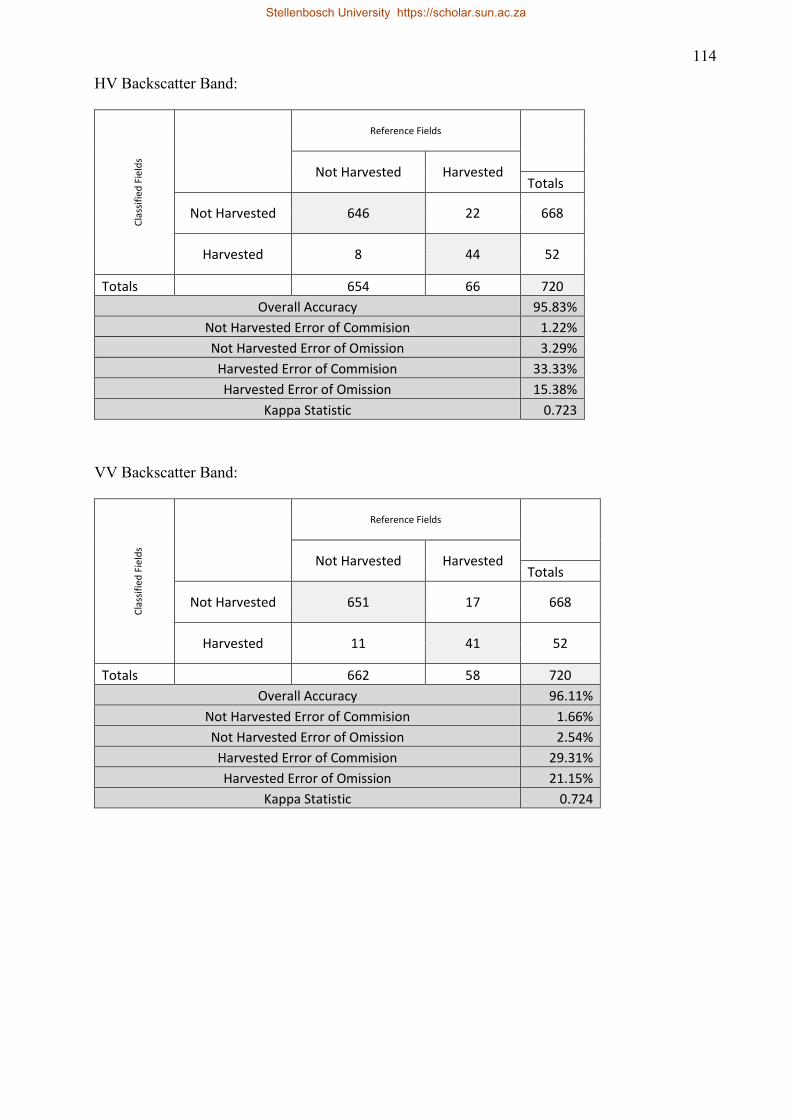
114

HV Backscatter Band:

Cla

ssif

ied

Fie

lds

Reference Fields


Totals


Harvested 8 44 52

Totals 654 66 720







VV Backscatter Band:

Cla

ssif

ied

Fie

lds

Reference Fields


Totals


Harvested 11 41 52

Totals 662 58 720








methods for sugarcane harvest detection using polarimetric sar · sugarcane, the growth period of...

Documents