methods for development of biologically effective

METHODS FORDEVELOPMENT OF

BIOLOGICALLYEFFECTIVE MANAGEMENT

STRATEGIES

North Dakota State UniversityDickinson Research Extension Center

2003

North Dakota State University 2003Dickinson Research Extension CenterRangeland Research Extension Program 4006

Methods for Development of Biologically Effective Management Strategies

Llewellyn L. Manske PhDRange Scientist

Project Assistants

Amy M. Kraus

Sheri A. Schneider


1089 State AvenueDickinson, North Dakota 58601

Tel. (701) 483-2076Fax. (701) 483-2073

North Dakota State University is an equal opportunity institute.

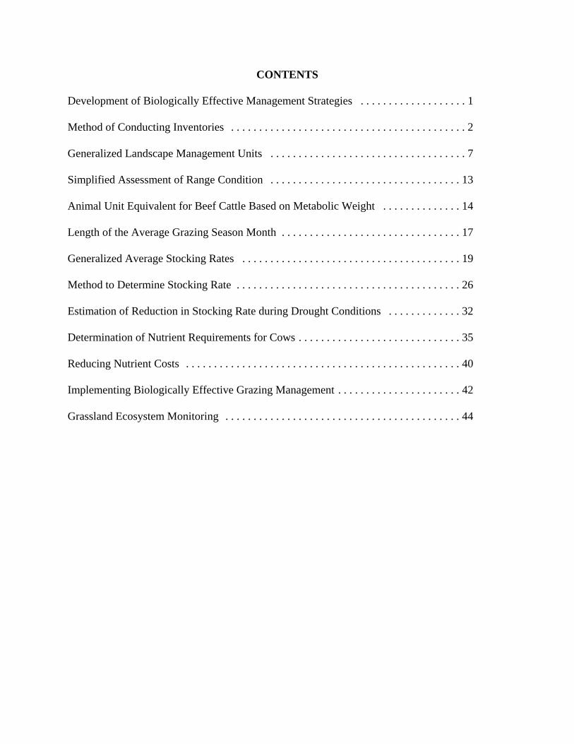
CONTENTS

Development of Biologically Effective Management Strategies . . . . . . . . . . . . . . . . . . . 1

Method of Conducting Inventories . . . . . . . . . . . . . . . . . . . . . . . . . . . . . . . . . . . . . . . . . . 2

Generalized Landscape Management Units . . . . . . . . . . . . . . . . . . . . . . . . . . . . . . . . . . . 7

Simplified Assessment of Range Condition . . . . . . . . . . . . . . . . . . . . . . . . . . . . . . . . . . 13

Animal Unit Equivalent for Beef Cattle Based on Metabolic Weight . . . . . . . . . . . . . . 14

Length of the Average Grazing Season Month . . . . . . . . . . . . . . . . . . . . . . . . . . . . . . . . 17

Generalized Average Stocking Rates . . . . . . . . . . . . . . . . . . . . . . . . . . . . . . . . . . . . . . . 19

Method to Determine Stocking Rate . . . . . . . . . . . . . . . . . . . . . . . . . . . . . . . . . . . . . . . . 26

Estimation of Reduction in Stocking Rate during Drought Conditions . . . . . . . . . . . . . 32

Determination of Nutrient Requirements for Cows . . . . . . . . . . . . . . . . . . . . . . . . . . . . . 35

Reducing Nutrient Costs . . . . . . . . . . . . . . . . . . . . . . . . . . . . . . . . . . . . . . . . . . . . . . . . . 40

Implementing Biologically Effective Grazing Management . . . . . . . . . . . . . . . . . . . . . . 42

Grassland Ecosystem Monitoring . . . . . . . . . . . . . . . . . . . . . . . . . . . . . . . . . . . . . . . . . . 44

1

Development of Biologically Effective Management Strategies



Grasslands that are not performing close totheir potential reduce the profit margins from theproduction of beef. Healthy grassland ecosystemsproduce greater quantities of herbage and morepounds of calf per acre than grasslands in goodcondition. The result is greater profit margins onhealthy grasslands. Improving grasslands from anaverage condition to a healthy status

• increases herbage production• reduces acres per cow-calf pair per month• reduces pasture costs per year• reduces feed costs per day• increases calf weight gain• increases calf weaning weight• reduces cost per pound of calf gain• increases net return per cow-calf pair• increases net return per acre• improves wildlife habitat, water and air quality,

and aesthetic quality.

Improving the health performance status ofgrassland ecosystems requires two steps: first, implementing biologically effective grazingmanagement practices that meet the biologicalrequirements of the plants and that coordinate grazingperiods with grass growth stages so that bothvegetative reproduction by tillering and activity ofrhizosphere organisms are stimulated, and second,monitoring the response of grassland ecosystemperformance to the changes in management practices. The response of biological mechanisms andecosystem processes to changes in managementstrategy is slow, and the response of grasslandecosystem performance to management practicesoccurs in annual incremental changes, both positiveand negative, which may be evident only throughannual monitoring.

Management practices that focus on meetingthe biological requirements of plants can sustain ahealthy grassland ecosystem over time. Theperformance levels of the plant component of agrassland ecosystem regulate the performance levelsof all the other components of the ecosystem. Plantsare the primary producers, converting light energyinto chemical energy during photosynthesis. Thiscaptured solar energy is the primary force driving all

ecosystem functions and provides the foundation forall uses of grasslands. By meeting the biologicalrequirements of the plants and facilitating theoperation of ecological processes at potential levels,proper management practices improve theperformance levels of all grassland ecosystemcomponents or maintain the health status andproductivity of a grassland ecosystem functioning athigh performance levels.

Monitoring the changes in the performancelevels of several components of the grasslandecosystem over time provides indirect indication ofthe status of grassland ecosystem health. Grasslandecosystem monitoring can be accomplished rapidlyand inexpensively through the use of the grasslandecosystem monitoring (GEM) method developed byNorth Dakota State University range scientists. Thismethod comprises three simple procedures: takingplot photographs, compiling a major plant speciespresent list, and completing a health statusassessment. Ecosystem components consideredduring health status assessment procedures areaboveground vegetation, belowground plantstructures, soil development processes, levels andtypes of erosion, ecological processes, andprecipitation infiltration. With the grasslandecosystem monitoring procedures, ranchers cancollect nonscientific, nonquantitative information thatcan be used to assess the performance status ofgrassland ecosystems, document changes in theecosystem, and evaluate the effectiveness ofmanagement practices.

Implementation of beneficial managementpractices will improve the status of grasslandecosystem health, and annual monitoring will allowmanagers to evaluate changes in performance levelsand to adjust management practices to ensure that thegrassland ecosystems are functioning at highperformance levels. Strengthening the status ofhealth of the grassland ecosystem will provideimprovement in livestock weight performance,reductions in livestock production costs, andincreases in profit margins.

2

A Method of Conducting Pasture and Forage Inventories to Be Used in the Development of Biologically Effective Management Strategies



The goal of a biologically effective pastureand forage management strategy is to match theforage quantity and nutritional needs of the livestockwith the herbage production curves and the nutrient-available curves of the various forage types so thatthe combination of forage types provides efficient useof the ranch natural resources. Development of abiologically effective pasture and forage managementstrategy for a ranch requires knowledge of the currentquantity and quality of the available pasture andforage types. A pasture and forage inventory isneeded to identify the resource types that will providethe forage needs of the livestock at their variousproduction stages.

A major goal of the inventory is to identifythe pasture and forage assets of the ranch and toidentify the features that cause bottlenecks restrictingthe management unit from reaching its optimumpotential production levels. The strongest pastureand forage asset of the ranch is the resource thatdetermines what the ceiling for the livestock numberswould be if the resource were used during itsoptimum period and if the forage types used duringthe other livestock production stages could bebrought up to an equivalent level. The bottleneckasset is the resource that limits livestock productionand shows what the potential bottom for the livestocknumbers would be if this problem were not corrected. The development of a biologically effectivemanagement strategy requires adjustments in thequantities of the natural resource types so that theneeds of the livestock can be met efficiently duringthe entire 12-month period.

A pasture and forage inventory is a list ofinformation about each parcel of land included in alivestock production operation. The main categoriesare pasture land, including native rangeland anddomesticated perennial grass; hayland, includingnative rangeland, domesticated grass, and alfalfa; andcropland, including grazed annual forage, annualforage hay, and annual crops for grain used for feedor cash sale. The information needed for hayland andcropland inventory includes the size in acres, foragetype, and average yield in tons per acre or bushels peracre. The information needed for pasture landinventory includes the size in acres, stocking rate in

ac/AUM, and carrying capacity in AUM’s of availableforage. A worksheet will help organize the pastureland information.

One of the major causes of low profit marginsfrom livestock production is the inefficiency ofcapturing economic value from the land resourcesinherent in old-style traditional management practices;in addition, the common practice of changing livestockforage sources on short notice or in crisis situations isexpensive. Increasing the economic value capturedfrom the land requires effective planning. One of thefirst steps in this planning process is to designatespecific parcels of land for forage production for eachgroup of livestock.

The pasture location of livestock groupsshould be predetermined for an entire year. A monthlytime line for livestock inventory worksheet is a usefulplanning tool. This worksheet is a planning list ofeach category of livestock, the number of livestock ineach category, and the pasture name or forage typeused for feed on a monthly schedule.

If gathering information for this worksheet ispart of the initial stages of changing pasture and foragemanagement from traditional practices to biologicallyeffective methods, a monthly time line for livestockinventory should be completed according to the old-style management practices. After a biologicallyeffective management plan is developed, a secondmonthly time line for livestock inventory should becompleted.

Worksheets for the methods described in thisreport should be copied before procedures are begun.

Acknowledgment

I am grateful to Amy M. Kraus for assistancein preparation of this manuscript. I am grateful toSheri Schneider for assistance in production of thismanuscript.

3

Steps in conducting a pasture and forage inventory for pasture land.

1. List pasture by name or number.

2. List total acreage of pasture.

3. List vegetation types in pasture (for example, native rangeland, crested wheat, smooth brome).

4. List acreage of each vegetation type in pasture.

5. List landscape sites in pasture (for example, lowland, upland, xeric) (see page 7, Generalized landscapesite management units).

6. Estimate percentage of each landscape site in pasture.

7. Determine acreage of each landscape site in pasture by multiplying total pasture acres (Step 2) by % landscape site (Step 6).

8. Identify range condition as one of four broad categories of condition: excellent, good, fair, or poor (seepage 13, Simplified assessment of range condition).

9. Determine stocking rates (ac/AUM) of landscape sites from average stocking rate value in ac/AUM tables(see page 19, Generalized average stocking rates).

10. Determine carrying capacity in AUM’s by dividing the acreage of each landscape site (Step 7) by averagestocking rate (Step 9).

11. Determine historical stocking rate (ac/AUM) for pasture by simple method (see page 24, Generalizedaverage stocking rate).

12. Determine historical carrying capacity in AUM’s by dividing total pasture acres (Step 2) by historicalstocking rate (Step 11).

Example of Pasture Land Inventory

To illustrate how to fill out the pasture and forage inventory worksheet for a ranch, we will use an exampleof a West River Region pasture of one section (640 acres) with 10% crested wheat and 10% lowland, 50% upland,and 30% xeric landscape sites. The area is grazed for 4.5 months, from 1 June to 15 October, by 70 cow-calf pairswith the cow average weight at 1,000 pounds.

Pasture and Forage Inventory Worksheet

(1) (2) (3) (4) (5) (6) (7) (8) (9) (10) (11) (12)

PastureName

Pasture TotalAcres

Vegetation Type

Vegetation TypeAcres

Landscape Site Range

Condition

Determined Historical

Group % Acres Stockingrate

Carrying capacity

Stockingrate

Carryingcapacity

West 640 2.04 313.7

Crested 64 10 64 1.25 51.2 AUM’s

Native 576 Lowland 10 64 Good 1.25 51.2

Upland 50 320 Good 2.00 160.0

Xeric 30 192 Good 4.00 48.0

310.4

AUM’s

Pasture and Forage Inventory Worksheet

(1) (2) (3) (4) (5) (6) (7) (8) (9) (10) (11) (12)

PastureName

Pasture TotalAcres

Vegetation Type

Vegetation TypeAcres

Landscape Site Range

Condition

Determined Historical

Group % Acres Stockingrate

Carrying capacity

Stockingrate

Carryingcapacity

6

Steps in conducting monthly time line for livestock inventory.

1. Separate livestock into production categories.2. List the number of head in each category for each month.3. List the pasture name or forage type that each livestock category is planned to use for feed for each month.

Monthly Time Line for Livestock Inventory Worksheet

Identify number of head and pasture location per month

Jan Feb Mar Apr May Jun Jul Aug Sep Oct Nov Dec

Mature Cows (A) 4's +

#head

Pasture

Mature Cows (B) 4's +

#head

Pasture

Mature Cows (C) 4's +

#head

Pasture

Young Cows2's, 3's

#head

Pasture

ReplacementHeifers

#head

Pasture

WeanedHeifers

#head

Pasture

Weaned Steers

#head

Pasture

Bulls #head

Pasture

Horses(AUE X 1.5)

#head

Pasture

Sick #head

Pasture

Other #head

Pasture

7

Range Sites Grouped into GeneralizedLandscape Management Units



Range site is the basic unit of rangeland withsimilar characteristics. Each named range site hassimilar soil characteristics, topographic position,environmental factors, and potential native vegetationcomposition. Range sites can be described andseparated to a finer degree than is practical forapplication of specific management practices. Theoretically, enough differences exist among therange sites to warrant the use of differentmanagement and stocking rates for each range site. Such specific management requires that each rangesite be identified and considered separately but as apart of the entire grassland management unit.

Classification of individual range sites for agrassland management unit is a complex process thatrequires the use of soil survey maps, soil seriesdescriptions, soil map unit descriptions, and rangesite descriptions. Most grassland mangers have nothad and most likely will not have a detailed range siteidentification completed for their land. However,completion of some level of range site identificationis a critical step in the development of a pasture andforage inventory.

Management of each range site separately isimpractical in most grazingland pasture situations. Range sites with similar levels of soil water andherbage production can be grouped into threegeneralized landscape site management units tosimplify grazingland management of pastures in theNorthern Plains.

This report attempts to simplify the processof range site identification by grouping categories ofrange sites into landscapes sites with similarmanagement requirements and similar stocking rates. Two major differences among the landscape sitemanagement units are the type of soil parent materialand the average annual precipitation. The averageannual precipitation and the types of parent materialfrom which soils have developed are variable acrossthe Northern Plains and form four distinctphysiographic regions: the Red River Valley, theDrift Prairie, the Missouri Coteau, and the WestRiver Regions.

The Red River Valley Region, part of theCentral Lowland Physiographic Province, is anexceptionally flat plain of glacial lake sedimentarydeposits and is characterized by very gentle slopesover 95% of the area. The region has poorlydeveloped stream systems. The range of averageannual precipitation is 18 to 20 inches. The majornative vegetation is the Bluestem, Switchgrass, andIndiangrass Type of the Tall Grass Prairie. Most ofthis region has been converted to cropland, and onlyfragments of tall grass prairie vegetation remain. Management considerations for this region are notincluded in this report.

The Drift Prairie Region, part of the CentralLowland Physiographic Province, is characterized byrolling, hummocky, or hilly glacial till deposits; gentleslopes of less than 8% on more than 80% of the area;and relief generally of less than 100 feet. The hills areclosely spaced, with valleys containing numerousclosed depressions called pot holes. The region haspoorly developed stream systems. The range ofaverage annual precipitation is 16 to 20 inches. Themajor vegetation is the Wheatgrass, Bluestem, andNeedlegrass Type of the Mixed Grass Prairie. Thisregion is considered the transition zone between theTall Grass Prairie and the Mixed Grass Prairie.

The Missouri Coteau Region, part of theGreat Plains Physiographic Province, is the glaciatedportion of the Missouri Plateau. This region is ahummocky plain of terminal moraine and dead-icemoraine deposits and is characterized by gentle slopesof less than 8% on 50 to 80% of the area and reliefgenerally of 100 to 300 feet. Some portions of theregion are well drained with streams, and otherportions have depressions containing closed basinswith small bodies of water. The range of averageannual precipitation is 14 to 18 inches. The majornative vegetation is the Wheatgrass and NeedlegrassType of the Mixed Grass Prairie.

The West River Region, part of the GreatPlains Physiographic Province, is the unglaciatedportion of the Missouri Plateau. In this regionsedimentary deposits have been eroded and formedinto a rolling to hilly plain with large buttes. Theregion is characterized by gentle slopes of less than

8

8% on 50 to 80% of the area and relief generally of300 to 500 feet. The region is well drained with adeveloped stream system. On an 8- to 25-mile-wideand nearly 200-mile-long strip along the LittleMissouri River exists a subregion of badlands. Thissubregion is a rugged, deeply eroded, hilly area withgentle slopes of less than 8% on 20 to 50% of thearea and relief commonly over 500 feet. The range ofaverage annual precipitation is 13 to 16 inches for the region. The major native vegetation is theWheatgrass and Needlegrass Type of the MixedGrass Prairie.

The range sites within each of the differentphysiographic regions of the Northern Plains can begrouped into three landscape site categories based onthe soil water holding capacity and the position of thewater table. These three landscape site categories areeasily identified and can be used for pasture andforage inventories during the development ofbiologically effective pasture and forage managementstrategies. The three landscape site categories arelowland, upland, and xeric sites. The lowlandlandscape sites have high levels of soil water in therooting zone of the soil for most of the year. Becauseof water run in, these sites receive greater amounts ofwater than the precipitation levels. The uplandlandscape sites have well-drained soils and areusually below field capacity for much of the growingseason. The xeric landscape sites have restrictedwater infiltration or water-holding capacity, and formuch of the growing season, available soil water isbelow the potential to be gained from precipitation.

Among the physiographic regions, thecharacteristics of a landscape site type differ slightly. Therefore, management requirements and stockingrates differ slightly for areas of a particular landscapesite type located in different physiographic regions.

Lowland Landscape Sites for the Drift PrairieRegion

Topography is nearly level, low-lying swales, depressions, shallow basins, anddrainageways. Slopes are less than 3%. Soils aredeep and are poorly drained to moderately welldrained. Permeability is very slow, slow, moderatelyslow, or moderate. Available water capacity ismoderate, high, or very high. Lowland landscapesites receive additional amounts of water from run infrom higher land, surface runoff, flooding, and/orunderground seepage.

Upland Landscape Sites for the Drift PrairieRegion

Topography is nearly level to rolling, with some areas gently sloping to moderately steep.Slopes are mostly 1 to 15%, with some 3 to 25%. Soils are deep to moderately deep; most aremoderately well drained to well drained, and some areexcessively well drained. Permeability is slow,moderate, moderately rapid, or rapid. Available watercapacity is low, moderate, or high.

Xeric Landscape Sites for the Drift Prairie Region

Topography is nearly level, undulating, or gently sloping. Slopes are 1 to 6%. Soils are mostly very shallow or shallow; some are deep. Mostare poorly drained or moderately well drained; someare excessively drained. Permeability is very slow,moderate, moderately rapid, or rapid. Available watercapacity is very low, low, or moderate. Most xericlandscape sites have thin surface soils with anunderlying hardpan that is nearly impervious to water.

Lowland Landscape Sites of the Missouri CoteauRegion

Topography is nearly level swales, basins,and depressions, or nearly level and gently undulatinglow-lying bottomlands and stream terraces. Slopes areless than 3%. Soils are deep and poorly drained. Permeability is very slow to moderate. Availablewater capacity is moderate, high, or very high. Lowland landscape sites receive additional amounts ofwater from run in from higher land, surface runoff,flooding, and/or underground seepage. Lowlandlandscape sites are usually briefly flooded, with waterstanding over the surface for part of the growingseason, and have a high water table for the majority ofthe growing season. Some lowland landscape siteshave surface areas with salts, and some have sodiumeffects throughout the profile.

Upland Landscape Sites of the Missouri CoteauRegion

Topography is nearly level, rolling, undulating, gently sloping, strongly sloping, or steep. Slopes are 1 to 35%. Soils are deep and moderatelydeep to shallow and are moderately well drained, welldrained, or excessively drained. Permeability is slow,moderate, moderately rapid, or rapid. Available watercapacity is low, moderate, or high. Upland landscapesites are usually underlain by sand, gravel, orweathered bedrock that restricts plant root penetration.

9

Xeric Landscape Sites of the Missouri CoteauRegion

Topography is nearly level, undulating, gently sloping, or strongly sloping. Slopes are 1to 9%. Soils are very shallow, shallow, or deep, andare well drained or excessively drained. Permeabilityis very slow, slow, moderate, or rapid. Available water capacity is low to moderate. Xeric landscape sites are usually underlain by sand or gravel or byhardpan that contains high accumulations of sodiumand is nearly impervious to water.

Lowland Landscape Sites of the West RiverRegion

Topography is slightly concave basins and depressions or nearly level low terraces and flood plains along streams and channels. Slopes are 1to 3%. Soils are deep and are poorly drained to welldrained. Permeability is very slow, slow, ormoderate. Available water capacity is low, moderate,high, or very high. Lowland landscape sites receiveadditional amounts of water from run in from higherland, surface runoff, flooding, and/or undergroundseepage. The water table is at the surface for theearly part of the growing season and remains high formost of the growing season. Some lowlandlandscape sites are saline and/or alkaline andcalcareous with salts at the surface and sodiumeffects throughout the profile.

Upland Landscape Sites of the West River Region

Topography is nearly level, undulating, rolling, gently sloping, or strongly sloping. Slopes are mostly 1 to 15%, with some 25 to 50%. Soils are deep, moderately deep, or shallow, and arewell drained to excessively drained. Permeability ismoderately slow, moderate, moderately rapid, or rapid. Available water capacity is low, moderate, or high. Upland landscape sites are underlain by shale,siltstone, or sandstone that restricts root depth.

Xeric Landscape Sites of the West River Region

Topography is nearly level, undulating, gently sloping, moderately sloping, or steep plains. Slopes are mostly 1 to 9%, and some are 2 to35%. Soils are very shallow or shallow. Permeabilityis moderate to very rapid near the surface and veryslow to slow in the substratum. Available watercapacity is very low, low, or moderate. Xericlandscape sites have thin surface soils underlain bycoarse sand, gravel, weathered bedrock, scoria, or by ahardpan that has a high accumulation of sodium and isnearly impervious to water. These substratummaterials restrict plant root depth.

Acknowledgment

I am grateful to Amy M. Kraus for assistancein preparation of this manuscript. I am grateful toSheri Schneider for assistance in production of thismanuscript.

10

Table 1. Range sites composing landscape site management units.

Lowland Landscape Sites

Wetland range site

Wet Meadow range site

Subirrigated range site

Overflow range site

Closed Depression range site

Saline Lowland range site

Upland Landscape Sites

Sands range site

Sandy range site

Silty range site

Clayey range site

Shallow range site

Thin Upland range site

Thin Sands range site

Xeric Landscape Sites

Shallow to Gravel range site

Shallow Clay range site

Claypan range site

Thin Claypan range site

Very Shallow range site

11

Table 2. Major grasses of landscape sites.


Western wheatgrass Agropyron smithii

Big bluestem Andropogon gerardi

Northern reedgrass Calamagrostis stricta

Canada wildrye Elymus canadensis

Switchgrass Panicum virgatum

Reed canarygrass Phalaris arundinacea

Sprangletop Scolochloa festucacea

Indiangrass Sorghastrum nutans

Prairie cordgrass Spartina pectinata

Slough sedge Carex atherodes

Wooly sedge Carex lanuginosa

Lowland sedges Carex spp.

Saline Lowland Landscape sites

Inland saltgrass Distichlis spicata

Foxtail barley Hordeum jubatum

Nuttall alkaligrass Puccinellia nuttalliana

Tumblegrass Schedonnardus paniculatus

Squirreltail Sitanion hystrix

Alkali cordgrass Spartina gracilis

12

Table 2. (Continued) Major grasses of landscape sites.



Sand bluestem Andropogon hallii

Sideoats grama Bouteloua curtipendula

Blue grama Bouteloua gracilis

Plains reedgrass Calamagrostis montanensis

Prairie sandreed Calamovilfa longifolia

Prairie junegrass Koeleria pyramidata

Little bluestem Schizachyrium scoparium

Sand dropseed Sporobolus cryptandrus

Needle and thread Stipa comata

Porcupine grass Stipa spartea

Green needlegrass Stipa viridula

Upland sedges Carex spp.




Buffalograss Buchloe dactyloides


Plains muhly Muhlenbergia cuspidata

Sandberg bluegrass Poa sandbergii

Little bluestem Schizachyrium scoparium




13

Simplified Assessment of Range Condition



Rangeland management and land useplanning require a system for assessing the health ofparcels of land. Range evaluation is essential toassess the effectiveness of implemented practices andto identify the ecological problems in a grasslandbefore its condition becomes seriously degraded. Thedevelopment of the concepts used in rangelandcondition assessment started about 100 years agowith the introduction of the concept of plantsuccession. Most succeeding methods have basedassessment primarily on the condition of thevegetation and soil compared to the degree ofdifference from a standard. Only recently has theapproach changed to base the assessment of the statusof rangeland health on the functional levels of theecological processes and the integrity of thevegetation, the soil, the air, and the water composingthe ecosystem.

Several interactive components of agrassland ecosystem should be considered duringgeneral condition assessment procedures: the statusof the aboveground and belowground vegetation; thestatus of soil development processes; the status of the levels and types of erosion; the status of ecological processes; and the status of precipitation infiltration. These major ecosystem components vary in degree ofperformance and level of functional status ongrasslands at different health conditions, and thechanges can be used as evaluation criteria for rankingrange condition categories.

Most range condition assessment methodsseparate the relative rankings of the performance andhealth of rangeland ecosystems into four conditioncategories from extremely healthy to extremelyunhealthy. The most commonly used conditioncategory names are excellent, good, fair, and poor.

The four general health condition categoriesshould be used in this preliminary estimatedassessment of grasslands based on the producer’sprevious experience and knowledge of the parcels ofland. The four range condition categories can beillustrated by comparison to human health condition. A grassland ecosystem in excellent condition is like ahighly trained athlete: highly productive, with allprocesses functioning at high rates and highefficiency; able to endure considerable stress; and

capable of rebounding from stress quickly. Agrassland ecosystem in good condition is like aperson in average health: productive, with allprocesses functioning at moderate rates and moderateefficiency; able to endure some stress; and capable ofgradual recovery from stress. A grassland ecosystemin fair condition is like a couch potato: marginallyproductive, with all processes functioning at low ratesand reduced efficiency; able to endure only minimalstress; and requiring long periods to recover fromstress. A grassland ecosystem in poor condition islike a chronically ill person: unproductive, with allprocesses functioning ineffectively and inefficiently;unable to endure stress; and capable of recoveringfrom stress only over considerable time and withspecial treatment.

Each parcel of land in a management planshould be placed into one of the four health conditioncategories based on the producer’s objectiveobservations during the past years of managing it. Only a few parcels of land in the Northern Plains arein the excellent and poor condition categories. Mostgrasslands are in either the good or fair conditioncategory. The main separation between good and fairis the relative amount of herbage produced bydesirable and less desirable species and the length oftime needed to recover from stress.

A report explaining the field methods for theassessment of rangeland health status frommonitoring plots located in each pasture is availableat http://www.ag.ndsu.nodak.edu/dickinso/research/2001/range01j.htm.

Acknowledgment

I am grateful to Amy M. Kraus forassistance in preparation of this manuscript. I amgrateful to Sheri Schneider for assistance inproduction of this manuscript.

14

Animal Unit Equivalent for Beef Cattle Based on Metabolic Weight



Should producers allocate more grass tolarge cows than to cows of average size duringplanning of grazing management strategies?

Body size affects the quantity of dry matterintake. Large cows eat more forage than do cows ofaverage size. Numerous methods have been devisedto predict or plan for livestock demand for forage. Arough guideline for daily dry matter intake can beestimated relatively quickly by using 2% of bodyweight (Holechek et al. 1989). This technique isuseful for general decisions, but when used toestimate forage needs in a grazing system, it tends tounderestimate the forage needs of lighter animals andoverestimate the forage needs of heavier animals.

A more accurate estimate of daily ormonthly forage demand of livestock on a grazingsystem can be reached by using the metabolic weightof the livestock rather than the live weight of theanimals. It has been found that metabolic weightaccounts for significant variation in dry matter intakeamong animals of different sizes (NRC 1996). Metabolic weight is the live weight to the 0.75 power. Beef cattle animal unit equivalents can be determinedfor animals of different sizes by calculating theirmetabolic weight as a percentage of the metabolicweight of a 1000-pound cow. A 1000-pound cowwith or without a calf is defined as 1.00 animal unit,which has a daily dry matter allocation of 26 poundsof forage.

Table 1 lists the calculated animal unitequivalents based on metabolic weight for a widerange of live animal weights. Calculating the animalunit equivalent for each cow in a herd would yield anaccurate estimate of the quantity of forage requiredby grazing livestock; however, this does not seempractical or necessary for proper management of agrazing system. But increasing the accuracy of theforage demand estimate by grouping similarly sized

animals of a herd into a few size categories andassigning appropriate animal unit equivalents to eachgroup does seem practical and beneficial. This wouldenable the manager to allocate the pasture forageresources more accurately. Table 2 suggests a fewbeef cattle size categories and corresponding animalunit equivalents that could be used for planninggrazing management strategies.

15

Table 1. Animal Unit Equivalent (AUE) based on metabolic weight (live animal weight 0.75).

Animal Live Weight

(lbs)

Animal UnitEquivalent yx 0.75

(% of 1000 lbs)

600 0.682

650 0.724

700 0.765

750 0.806

800 0.846

850 0.885

900 0.924

950 0.962

1000 1.000

1100 1.074

1200 1.147

1300 1.217

1400 1.287

1500 1.355

1600 1.423

1700 1.489

1800 1.554

1900 1.618

2000 1.682

2200 1.806

2400 1.928

2600 2.048

2800 2.165

3000 2.280

16

Table 2. Suggested practical application of Animal Unit Equivalent based on metabolic weight (live animal weight 0.75).

Beef Animal Category Animal Unit Equivalent

Weaned animal lighter than 800 lbs 0.75

Young animal 800-900 lbs 0.85

Cow 900-1100 lbs with calf 1.00

Cow 1100-1300 lbs with calf 1.15

Cow heavier than 1300 lbs with calf 1.25

Bull lighter than 2000 lbs 1.50

Bull heavier than 2000 lbs 2.00

Definitions from Society for Range Management Glossary, Jacoby, Chair., 1989.

Animal-unit. Considered to be one mature cow of approximately 1,000 pounds, either dry or with calfup to 6 months of age, or their equivalent, based on a standardized amount of forage consumed.

Animal-unit-month. The amount of dry forage required by one animal unit for one month based on aforage allowance of 26 pounds per day.

Literature Cited

Holechek, J.L., R.D. Pieper, and C.H. Herbel. 1989. Range management principles and practices. Prentice Hall, NJ.

National Research Council. 1996. Nutrientrequirements of beef cattle. Seventhrevised edition. National AcademyPress, Washington DC.

17

Length of the Average Grazing Season Month



When designing grazing managementstrategies, range managers need to know the numberof days in the average grazing season month in orderto calculate the number of cow-calf pairs to turn outonto a pasture. The calculation is based on the size ofthe pasture in acres (AC), the evaluated stocking ratepotential (acres (AC)/animal unit month (AUM)), andthe number of days in the grazing season (convertedto months (M)):

Total number of pasture acres (AC) ÷evaluated stocking rate (AC/AUM) ÷ lengthof grazing season in months (M) = number of cow-calf pairs (AU)

An animal unit (AU) is the equivalent of one maturecow of about 1000 pounds, with or without a calf. An animal unit month (AUM) is the amount of foragedry matter required by one animal unit (AU) for 1month (M). The length of the grazing season inmonths is calculated by dividing the number of daysin the grazing season by the number of days in theaverage grazing season month. How many days arein the average grazing season month? Thisseemingly superficial question does not have a simpleanswer, and because of its importance to rangemanagers, this question should be given carefulconsideration. Currently, three values for the lengthof an average grazing season month are usedrelatively indiscriminately: 30 days, 30.5 days, and31 days.

The results of calculations of the number ofcow-calf pairs to be turned onto a pasture are greatlyaffected by the value used for the length of anaverage month. For example, the solution to theequation determining the number of cow-calf pairs tobe supported on a pasture that covers 3840 acres, hasa potential stocking rate of 3.0AC/AUM, and is to begrazed seasonlong for 183 days, from 16 May to 15November, would vary according to different averagemonth lengths used. The calculations would indicatethat the number of cow-calf pairs to be turned outonto this pasture would be 210 pairs if 30 days permonth (183d ÷ 30d = 6.1M) were used, 213 pairs if30.5 days per month (183d ÷ 30.5d = 6.0M) wereused, and 217 pairs if 31 days per month (183d ÷ 31d= 5.9M) were used. This paper will attempt topresent justifications for the acceptance of one value

for the length of an average grazing season monthand for its uniform use in calculations applied tograzing in the Northern Plains.

The earth completes 1 rotation on its axis ina period of time called a day. The earth revolvesaround the sun in a period of time called a year. Oneyear is equal to 365.2425 days. The additionalquarter of a day is corrected by adding 1 day every4th year. In our calendar, each year comprises 12months: 7 with 31 days, 4 with 30 days, and 1 with28 days for 3 years and 29 days every 4th year. There are 1461 days in a cycle of 48 months. Theaverage month in this 4-year cycle contains 30.44days. This would be an accurate value to use incalculating stocking rates of grazing systems in areasthat graze 12 months per year.

The climate in the Northern Plains does notpermit grazing for 12 months, however. In thecalculation of the average length of a grazing seasonmonth, a logical practice would be to eliminate fromthe data set the months during which grazing does notoccur. Debate exists over the period to be consideredgrazing season months in the Northern Plains, and thedetermination depends on specific situations,including available forage types and managementstrategy applied. The length of the average grazingseason month could range from 30.3 days to 30.7days, depending on which months were selected. Theprobability of occurrences of inclement weatherconditions is high in December, January, February,and March; these months are also characterized byaverage monthly temperatures too low to supportplant growth. Grazing during this 4-month periodwould not be dependable. The active growing seasonfor perennial plants is from about mid April to midOctober. The 8-month period of April throughNovember has the potential to have some livestockgrazing, although grazing during this time is notrecommended as a universal practice. This periodhas 244 days and an average month length of 30.5days.

The results of the practical application of theaverage month length in a 4-year cycle and of the average month length in the 8-month grazingseason in the Northern Plains are the same. In theexample presented earlier, if 30.44 days were the

18

value used for the average month length, thecalculation would indicate that 213 cow-calf pairsshould be turned onto the pasture (3840AC ÷3.0AC/AUM ÷ 6.01M = 212.91 AU). Likewise, ifthe value used for the average month length were30.5 days, the calculation would indicate that 213cow-calf pairs should be turned onto the pasture(3840AC ÷ 3.0AC/AUM ÷ 6.0M = 213.33 AU). Thispaper demonstrates that in calculations of stockingrates for grazing management strategies in theNorthern Plains, 30.5 days more accurately reflectsthe length of the average grazing season month than30 or 31 days.

Acknowledgment


19

Generalized Average Stocking Rates



Each piece of grassland can withstandgrazing to a certain biological level before negativeeffects occur. This biological level varies slightlywith amount of annual precipitation, ecologicalcondition of the grassland, and type of grazing systemused. Moving cattle from a pasture only when all theaboveground herbage has been removed is not asound management practice. To manage grasslandsproperly, the producer must know the number ofcows that can be grazed on a grassland unit for aspecified length of time. This number is termed thestocking rate.

Stocking rate is commonly stated as acresper animal unit month (AUM) or its reciprocal,AUM’s per acre. An animal unit month (AUM) isthe amount of dry forage one mature cow ofapproximately 1,000 pounds with a calf requires forone month.

Forage dry matter intake of grazing animalsis affected by the size of the cow. Large cowsconsume more forage than medium- and standard-sized cows. A more accurate estimate of daily ormonthly forage demand of livestock on grazinglandscan be determined with the metabolic weight of theanimal than with its live weight. Metabolic weight islive weight to the 0.75 power. A 1000-pound cowwith a calf is the standard, which is defined as 1.00animal unit (AU) and has a daily dry matterallocation of 26 pounds of pasture forage. Themetabolic weight of a 1200-pound cow with a calf is1.147 animal unit equivalent (AUE), which has adaily dry matter allocation of 30 pounds of pastureforage. The metabolic weight of a 1400-pound cowwith a calf is 1.287 animal unit equivalent (AUE),which has a daily dry matter allocation of 33 poundsof pasture forage. The amount of forage dry matterconsumed in one month by one animal unit, a 1000-pound cow with a calf, is an animal unit month(AUM). The daily dry matter allocation for a cowwith a calf on pasture is different from the daily drymatter requirement for just the cow during the sameproduction periods.

Determining stocking rate for a parcel ofgrassland by using range site identification and rangecondition assessment is a complex, time-consumingprocess. Most grassland managers have not had and

most likely will not have a detailed range stockingrate evaluation completed for their land. However,completion of some level of stocking rate evaluationis an essential step in the development of a pastureand forage inventory. This report summarizes thelong-term generalized stocking rate levels for threelandscape site management units in the Drift Prairie,Missouri Coteau, and West River Regions of theNorthern Plains (tables 1-3). The three landscape sitecategories are lowland, upland, and xeric landscapesites. The areas of each landscape site that arelocated in the three different physiographic regionshave slightly different average stocking rates. Theaverage stocking rates of the three landscape sites arehighly variable with changes in ecological rangecondition.

The stocking rate estimates in this reportassume that the grasslands are managed byseasonlong grazing for 4.5 to 5.0 months, June toOctober. If the grasslands are managed by 6-monthseasonlong grazing from mid May to mid November,the manager can expect the stocking rate to be 140%of the acres/AUM rate for the 4.5- to 5.0-monthseasonlong strategy. If the seasonlong grazing isstarted earlier than mid May and/or continued laterthan mid November, the manager can expect thestocking rate to be 200% or more of the acres/AUMrate for the 4.5- to 5.0-month seasonlong strategy.

The manager using a grazing system canexpect stocking rates higher than 4.5- to 5.0-monthseasonlong stocking rates (Manske 1995). Themanager using the deferred grazing system, on whichgrazing is delayed until after grass seed development,can expect the deferred pasture to support a stockingrate about 80% of the acres/AUM rate supported by a4.5- to 5.0-month seasonlong grazing strategy duringthe first 4 to 6 years. The manager using the shortduration grazing system can expect the stocking rateto be 75% of the acres/AUM rate supported by a 4.5-to 5.0-month seasonlong grazing strategy. Themanager using the twice-over rotation grazing systemcan expect the stocking rate to be 70% of theacres/AUM rate supported by a 4.5- to 5.0-monthseasonlong grazing strategy. A long-term, well-managed twice-over grazing system can support astocking rate about 55% of the acres/AUM rate of a4.5- to 5.0-month seasonlong grazing strategy.

20

The mean average stocking rates for theDrift Prairie, Missouri Coteau, and West RiverRegions’ lowland landscape sites of the good and faircondition categories are 1.10, 1.25, and 1.60acres/AUM, respectively, and the mean for the threeregions is 1.30 acres/AUM. The mean averagestocking rates for the Drift Prairie, Missouri Coteau,and West River Regions’ upland landscape sites ofthe good and fair condition categories are 1.75, 2.10and 2.50 acres/AUM, respectively, and the mean forthe three regions is 2.10 acres/AUM. The meanaverage stocking rates for the the Drift Prairie,Missouri Coteau, and West River Regions’ xericlandscape sites of the good and fair conditioncategories are 2.90, 3.65, and 5.00 acres/AUM,respectively, and the mean for the three regions is3.85 acres/AUM.

Much of the Northern Plains’ nativerangeland has been grazed by domesticated livestockfor over 100 years. Knowledge of a grasslandparcel’s historical use is very valuable fordetermining the future stocking rates of thebiologically effective pasture and forage managementstrategies. Determining the historical stocking ratesfor a parcel of grassland is not difficult. The onlyinformation needed is the average number of daysgrazed and the number of cow-calf pairs grazedduring the recent past.

The first step is to convert the averagenumber of days to average length in months bydividing by 30.5, the average number of days in theaverage grazing season month (Manske 1998b). Thenext step is to determine the number of averageanimal unit months (AUM’s) of grazing. Each cow-calf pair is an animal unit. The number of animalunits (AU) multiplied by the number of months (M)will give the average total number of AUM’s for thatparcel of grassland. If the cows are larger than 1,000pounds, the animal units should be converted toanimal unit equivalents (AUE). The current methodused to convert AU to AUE is based on the metabolicweight of the animals. The AUE values for variouslive weights can be found on tables 1 and 2 of Manske 1998a (see pages 15 and 16).

Acknowledgment


Literature Cited

Manske, L.L. 1995. Economic returns as affectedby grazing strategies. NDSU DickinsonResearch Extension Center. Range ResearchReport DREC 95-1012. Dickinson, ND. 20p.

Manske, L.L. 1998a. Animal unit equivalent forbeef cattle based on metabolic weight. NDSU Dickinson Research Extension Center. Range Management Report DREC 98-1020. Dickinson, ND. 3p.

Manske, L.L. 1998b. How long is the averagegrazing season month? NDSU DickinsonResearch Extension Center. RangeManagement Report DREC 98-1021. Dickinson, ND. 2p.

21

Table 1. Generalized average stocking rates for 1000 lb cows (1.00 AUE) for the Drift Prairie (A), Missouri Coteau (B), and West River (C) Regions of the Northern Plains.

Stocking Rate in Acres/AUM (1000lb cow=1.00 AUE)

Range Condition Category

Landscape Units Excellent Good Fair Poor

A B C A B C A B C A B C

Lowland Landscape Sites 0.75 0.75 1.00 1.00 1.00 1.25 1.25 1.50 2.00 2.50 2.75 3.50

Upland Landscape Sites 1.00 1.25 1.50 1.50 1.75 2.00 2.00 2.50 3.00 4.00 5.00 6.00

Xeric Landscape Sites 1.75 2.25 3.00 2.25 3.00 4.00 3.50 4.25 6.00 7.00 8.00 11.0

Stocking Rate in AUM’s/Acre (1000lb cow=1.00 AUE)







22
















23
















24

To illustrate how to determine the historical stocking rate of a ranch, we will use an example of a pasture ofone section (640 acres) that has usually been grazed from 1 June to 15 October by 70 cow-calf pairs with the cowaverage weight at 1,000 pounds. The average historical stocking rate can be determined by a few easy steps.

1. Determine the grazing season length in months.

number of daysin total grazing season

÷

average number ofdays in grazing season months

=

number of monthsin grazing season

137 days ÷ 30.5 d = 4.5 M

2. Determine the number of animal units (AU).

Number of cow-calf pairs

X

animal unit equivalents

= Animal units (AU)

70 c-c prs X 1.0 AUE = 70 AU

3. Determine the total number of animal unit months (AUM’s).

Animal units (AU) X number of months = animal unit months (AUM’s)

70 AU X 4.5 M = 314 AUM’s

4a. Determine the average stocking rate in acres/AUM.

Pasture size in acres ÷ number of animal unit months = acres per AUM

640 acres ÷ 314 AUM’s = 2.04 ac/AUM

4b. Determine the average stocking rate in AUM’s/acre.

Animal unit months ÷ pasture acres = AUM’s per acre

314 AUM’s ÷ 640 acres = 0.49 AUM’s/ac

25

If the cows’ average weight is heavier than 1,300 pounds, the procedure is as follows:

1. Determine the grazing season length in months.

Use the same procedure as with 1,000-pound cows.

2. Determine the number of animal units (AU).

Number of cow-calf pairs

X

animal unit equivalents = Animal units (AU)

70 c-c prs X 1.25AUE = 87.5 AU

3. Determine the total number of animal unit months (AUMs).

Animal units (AU) X number of months = animal unit months (AUM’s)

87.5 AU X 4.5 M = 394 AUM’s

4a. Determine the average stocking rate in acres/AUM.

Pasture size in acres ÷ number of animal unit months = acres per AUM

640 acres ÷ 394 AUM = 1.62 ac/AUM

Three stocking rates for a parcel of grassland can serve as guidelines for the development of 12-month pastureand forage management strategies.

The mean average upland landscape sites’ stocking rate is 2.10 acres per AUM.The historical stocking rate for 1,000-pound cows is 2.04 acres per AUM.The historical stocking rate for 1,300-pound cows is 1.62 acres per AUM.These three stocking rate values should be evaluated in relation to the condition of the grassland parcel. If the

historical stocking rate is greater than the average stocking rate and the condition of the grassland is low good or fair,the producer should consider a change in grazing management system and/or stocking rate.

26

A Method of Determining Stocking Rate Based on Monthly Standing Herbage Biomass



Stocking rate is the number of animals(animal unit) for which a grassland unit (acre) canprovide adequate dry matter forage for a specifiedlength of time (month). Stocking rate depends on theamount of herbage biomass available to grazinganimals, the time of year, the type of grazing systemused, and the amount of forage consumed bylivestock per month. Stocking rate is commonlypresented as acres per animal unit month (AUM) orits reciprocal, AUM’s per acre.

Forage dry matter intake of grazing animalsis affected by the size of the cow. Large cowsconsume more forage than do medium- and standard-sized cows. A more accurate estimate of daily ormonthly forage demand of livestock on grazinglandscan be determined with the metabolic weight of theanimal than with its live weight. Metabolic weight islive weight to the 0.75 power. A 1000-pound cowwith a calf is the standard, which is defined as 1.00animal unit (AU) and has a daily dry matterallocation of 26 pounds of pasture forage. Themetabolic weight of a 1200-pound cow with a calf is1.147 animal unit equivalent (AUE), which has adaily dry matter allocation of 30 pounds of pastureforage. The metabolic weight of a 1400-pound cowwith a calf is 1.287 animal unit equivalent (AUE),which has a daily dry matter allocation of 33 poundsof pasture forage. The amount of forage dry matterconsumed in one month by one animal unit, a 1000-pound cow with a calf, is an animal unit month(AUM). The daily dry matter allocation for a cowwith a calf on pasture is different from the daily drymatter requirement for just the cow during the sameproduction periods. During the grazing season fromMay through November, the length of the averagemonth is 30.5 days.

The mathematical process used to determinestocking rate from herbage biomass is presented intable 1. The amount of herbage available during thegrazing season is the average value of the meanmonthly standing herbage biomass values for thegrazing-season months. The mean monthly standingherbage biomass should be determined by clippingand weighing the dry herbage from each pasture andaveraging the weights over several years. If thesevalues are not available, the generalized values for

western North Dakota native rangeland (table 2) canbe substituted. The general monthly herbage valueson the herbage weight curve in table 2 are averages ofherbage production on well-managed pastures duringyears with normal precipitation.

Each of the monthly herbage biomass valuesneeds to be adjusted to reflect the differing effects various grazing treatments have on the quantity ofherbage biomass produced. Time of year andintensity of defoliation vary with different grazingtreatments; these variations affect plant biologicalmechanisms and result in the production of differentamounts of herbage. The percentages of the potentialamount of herbage biomass produced on variousgrazing treatments are summarized in table 2. Themonthly herbage biomass values for the months ofthe grazing season can be adjusted for differences inherbage biomass on specific grazing treatments bymultiplying monthly herbage weight by thepercentage of potential herbage produced on aparticular grazing treatment.

The effects of drought conditions cansuppress herbage biomass production for 1 to 4 years,depending on the health status of plants prior to waterdeficiency periods. This reduction in herbageproduction must be reflected in the calculations todetermine accurate stocking rates during the droughtand recovery periods. These adjustments need not bedetermined for growing seasons in which herbagebiomass is not affected by current or previous droughtconditions.

Each of the monthly herbage biomass values during drought and during the perennial plantrecovery period needs to be adjusted to reflect thepercentage of herbage weight reduction that resultedfrom the effects of drought conditions. The percentreduction that results from the effects of droughtconditions can be determined by a comparison ofnormal-year herbage biomass and drought-year orrecovery-year herbage biomass. If these data are notavailable, estimations based on several years ofexperience can be used. The estimate of percentherbage reduction needs to be converted to percent ofherbage biomass produced. The percent of herbageproduced is determined by subtracting the percent

27

reduction in herbage from 100%. The monthlynormal-year herbage biomass values adjusted for theeffects of grazing system are multiplied by percent ofherbage produced to adjust for the effects of droughtconditions.

The average monthly herbage biomass isdetermined by adding the adjusted monthly herbagebiomass for the months of the grazing season anddividing the sum by the number of grazing-seasonmonths.

Not all of the average herbage biomass forthe planned months of the grazing season isconsumable forage. Perennial plants must retain aportion of the leaf material to conduct photosynthesisand provide carbohydrates and other productsnecessary to sustain healthy and productive growth. The amount of leaf material the plant must retainranges from 40% to 60%, depending on grasslandtype (40% on the shortgrass, 50% on the midgrass,and 60% on the tallgrass prairies). When specificvalues for percent proper utilization are not knownfor the grassland type, an average value of 50% maybe used. This value implies that the plant retains halfthe herbage and half the herbage is available forutilization.

Not all standing herbage available for properutilization is ingested by grazing animals. Grazinglivestock consume only about 50% of herbageavailable for utilization. The remainder of theutilized herbage is broken from the plant, soiled byanimal waste, consumed by insects and wildlife, andlost to other natural processes. Data to allowcomparison of forage-harvest efficiency on differentgrazing systems are not available. However, thequantity of herbage ingested by livestock would beexpected to increase with improvement in efficiencyof harvest from some grazing systems.

The differences in daily dry matter intake forcows of different weights are used to adjust stockingrates for cow size. The standard 1000-lb cowrequires 26 lbs of dry matter per day. The dry matterintake for lighter or heavier cows can be determinedby multiplying 26 lbs by the animal unit equivalent(table 3), which is based on the metabolic weight ofthe cow.

For determination of stocking rate, theavailable monthly forage for intake value adjusted forgrazing system and drought conditions is divided bythe amount of dry matter per cow per month--thedaily amount of dry matter per cow adjusted for cowsize and multiplied by the number of days peraverage month (30.5 days). This stocking rate is

presented as AUM’s per acre. The reciprocal can bedetermined by dividing that number into 1 to giveacres per AUM. This is the number of acres requiredto provide forage for one month for a cow with a calf.

Stocking rates vary with the amount ofherbage production and are determined from theaverage monthly herbage biomass for the months ofthe grazing season and the weight of the cows. Thequantity of the standing herbage in grassland pasturesis not constant during the period grazed. The weightof the herbage dry matter per acre increases duringthe early growth stages until the maximum plantheight is reached, and then the dry matter weightdecreases as the mature plants dry during senescence. Table 4 shows the stocking rates for different averagemonthly herbage biomass quantities and cow sizes.

The number of cows to turn onto the grazingsystem is determined by dividing the total number ofacres in the pastures of a grazing system by the acresper AUM value and dividing this total number ofAUM’s by the number of months of the grazingseason. The number of cows that can graze thepastures subtracted from the total number of cows inthe herd will show any forage shortfall.

The stocking rate value determined by thismathematical process is based on the averagemonthly standing herbage biomass for the grazing-season months and has been adjusted for percentageutilization, percentage forage intake, grazing system,cow size, and the effects of drought conditions.

Acknowledgment


28

Table 1. Process to determine stocking rate from monthly herbage biomass.

Adjustment for grazing treatment

Monthly herbage biomass value (from clipped and dried samples or from table 2) X % of potential herbageproduced on appropriate grazing treatment (from table 2)

Adjustment for effects of drought conditions

Monthly herbage biomass value adjusted for grazing treatment X (100 % - % herbage reduction)

Average monthly herbage biomass

Sum of adjusted monthly herbage biomass for the months of the grazing season

÷ number of grazing season months

Adjustment for size of cow

26 lbs daily dry matter intake X Animal Unit Equivalent for appropriate cow size (from table 3).

Stocking Rate

Average monthly herbage biomass adjusted for grazing treatment and for drought conditions

X % proper utilization (50%)

X % consumed (50%)

= lbs of available monthly forage

÷ dry matter per AUM (26 lbs X AUE X 30.5 days)

= AUM/ac

reciprocal1.0 ÷ AUM/ac = ac/AUM

The number of cows that can graze the available forage

Total number of acres in grazing system

÷ acres/AUM

÷ number of grazing season months

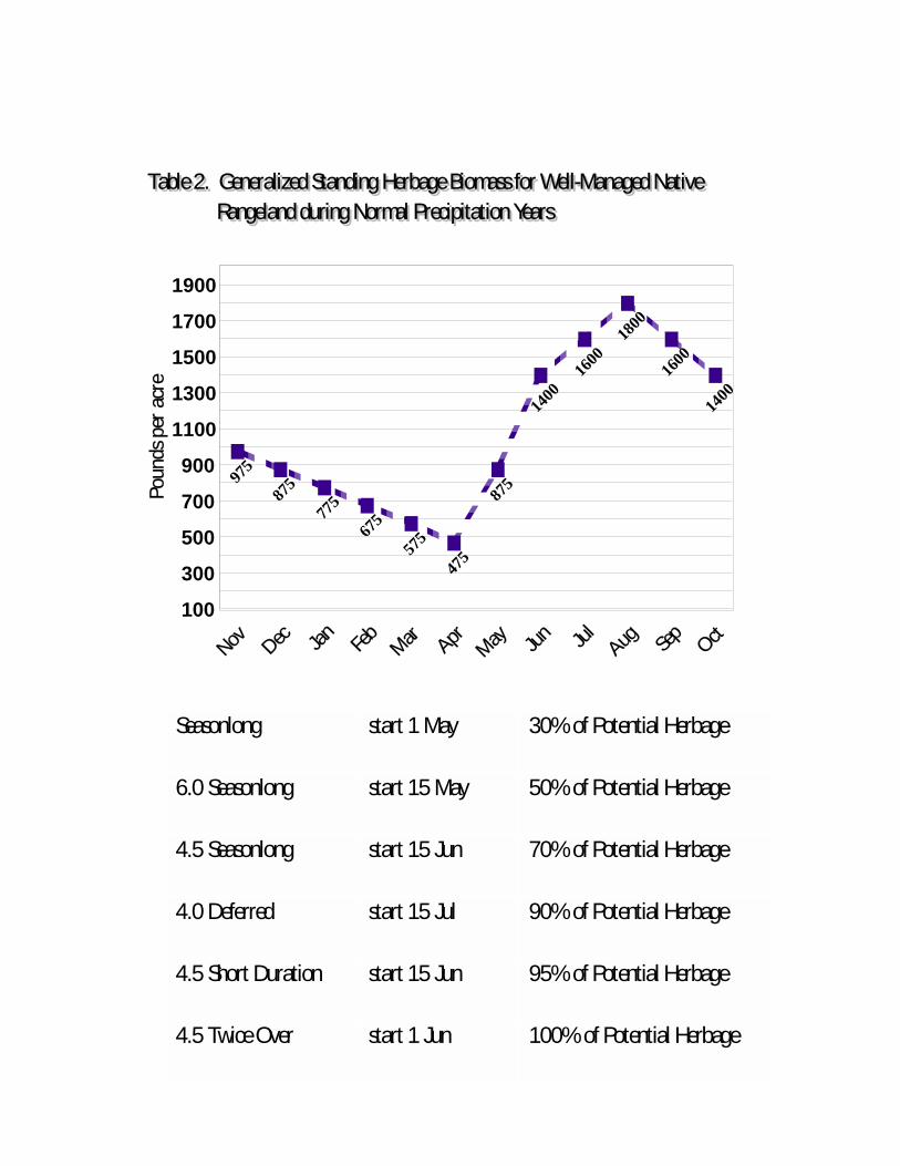
975

875

775

675

575

475

875

1400

1600

1800

1600

1400

Nov Dec Jan Feb

Mar AprMay Ju

n Jul

Aug Sep

Oct100

300

500

700

900

1100

1300

1500

1700

1900

Poun

ds p

er a

cre

Table 2. Generalized Standing Herbage Biomass for Well-Managed Native Table 2. Generalized Standing Herbage Biomass for Well-Managed Native Rangeland during Normal Precipitation Years Rangeland during Normal Precipitation Years

Seasonlong start 1 May 30% of Potential Herbage

6.0 Seasonlong start 15 May 50% of Potential Herbage

4.5 Seasonlong start 15 Jun 70% of Potential Herbage

4.0 Deferred start 15 Jul 90% of Potential Herbage

4.5 Short Duration start 15 Jun 95% of Potential Herbage

4.5 Twice Over start 1 Jun 100% of Potential Herbage

30

Table 3. Animal Unit Equivalent (AUE) based on metabolic weight (live animal weight 0.75 ).

Animal Live Weight

(lbs)

Animal UnitEquivalent yx 0.75

(% of 1000 lbs)

600 0.682

650 0.724

700 0.765

750 0.806

800 0.846

850 0.885

900 0.924

950 0.962

1000 1.000

1100 1.074

1200 1.147

1300 1.217

1400 1.287

1500 1.355

1600 1.423

1700 1.489

1800 1.554

1900 1.618

2000 1.682

2200 1.806

2400 1.928

2600 2.048

2800 2.165

3000 2.280

31

Table 4. Stocking rates (acre/AUM) for different quantities of average monthly herbage dry matter biomass (DM lb/acre) and three weights of cows.

Stocking Rates

acre/AUM

1000 lb CowsHerbage Biomass

DM lb/acre


DM lb/acre


DM lb/acre

1.00 3172 3660 4084

1.25 2538 2928 3267

1.50 2115 2440 2723

1.75 1813 2091 2334

2.00 1586 1830 2042

2.25 1410 1627 1815

2.50 1269 1464 1634

2.75 1153 1331 1485

3.00 1057 1220 1361

3.25 976 1126 1257

3.50 906 1046 1167

3.75 846 976 1089

4.00 793 915 1021

4.25 746 861 961

4.50 705 813 908

4.75 668 771 860

5.00 634 732 817

32

Procedure to Estimate Percent Reduction in Stocking Rate during Drought Conditions



Stocking rates are affected by the amount ofherbage biomass plants produce. During periods ofbelow-normal precipitation, decreased herbageproduction may necessitate adjustments in stockingrates. The required percent reduction in the stockingrate can be estimated from the percent reduction inpeak herbage biomass in healthy plants.

Effective grazing management can helpminimize herbage reductions during periods ofbelow-normal precipitation because herbageproduction is affected by both the type ofmanagement practices used and the level ofprecipitation in relation to normal amounts. Thequantity of herbage biomass produced is related toplant size and plant density. These twocharacteristics are directly affected by the level ofplant health, which is determined by the biologicaleffectiveness of the management strategy used.

Management practices that do not meet thebiological requirements of the plants slow plantprocesses. The resulting deterioration in the level ofplant health is manifested as decreased plant densityand diminished plant size that lead to reducedherbage production during periods with normalprecipitation. Herbage reduction percentages causedby detrimental grazing management practices such asgrazing before the third-leaf stage, grazingseasonlong, or grazing during the fall usually varybetween 40 and 60 percent below the potentialherbage biomass. The greatest reductions in herbageproduction observed in western North Dakota haveoccurred on domesticated grass spring pastures thatwere hayed during the summer and/or grazed duringthe fall, on native rangeland summer pastures thatwere grazed during the fall, and on domesticatedgrass and alfalfa haylands that were hayed late and/orgrazed during the fall.

Herbage weight of perennial plants increasesfrom early season through May, June, and July untilpeak herbage biomass, which occurs during the lastcouple weeks of July. Herbage weight then decreasesas plants age and dry. The amount of herbagebiomass produced by healthy plants is related to precipitation levels during January through July,which affect plant size and plant density.

Herbage reduction percentages caused bylow precipitation are usually proportional to thelevels of precipitation below the normal range. Anestimate of the amount of herbage reduction lowprecipitation causes in healthy plants can bedetermined by a comparison between the local long-term mean precipitation received during Januarythrough July and the current year’s precipitation forthat period. The range of normal precipitation is plusor minus 25 percent of the long-term mean.

The procedure to estimate percent reductionin peak herbage biomass caused by below-normalprecipitation requires just three simple calculations:first, the monthly precipitation for January throughJuly is totaled to give the current seasonalprecipitation; then, this precipitation amount isdivided by the local long-term January through Julyprecipitation amount to determine the currentseasonal precipitation as a percentage of the long-term mean precipitation; next, that percentage issubtracted from 75 percent, which is the low-normallong-term precipitation value.

The resulting estimated percentage ofreduction that below-normal precipitation has causedin peak herbage biomass provides a guideline for thepercent reduction in stocking rate needed for theremainder of the grazing season--until mid October--on pastures that have been properly managed andhave healthy plants. For example, if the Januarythrough July seasonal precipitation amount is 65percent of the long-term mean, the estimated 10percent reduction from normal herbage biomasswould suggest a 10 percent reduction in stockingrate--assuming the proper stocking rate was beingused. This method does not determine the amount forstocking rate adjustments required on pasturesmanaged by practices that diminish the health statusof plants below potential levels.

The long-term mean monthly precipitationamounts for numerous locations are available on theNational Weather Service (NOAA) web site forNorth Dakota (www5.ncdc.noaa.gov/climatenormals/clim81/NDnorm.pdf). For the current season’sprecipitation, amounts collected at individual ranchesand marked on the calendar can be used if a completeJanuary through July data set is available. Another

33

source for the current season’s precipitation amountsfor many locations is the NDAWN web site(http://ndawn.ndsu.nodak.edu ). These data start inApril because NDAWN does not collect data forprecipitation that occurs as snow. The precipitationamounts for January through March and the amountof precipitation that falls as snow during otherperiods must be obtained from other sources. Currentseason’s precipitation data that include snow moistureamounts are available on the National WeatherService site (www.crh.noaa.gov/bis/OtherHydro.htm Click on “text” for the desired month’s precipitationdata).

If the percentages of reduction in herbagebiomass produced on domesticated grass springpastures, native rangeland pastures, or grass andalfalfa haylands are greater than the estimatedpercentage of herbage reduction reached by thecomparison between the long-term and currentseasonal precipitation amounts, the health of theplants is below the potential level becausemanagement practices have not met the plantbiological requirements. When managementpractices meet the biological requirements of theplants and the level of plant health is high, thepercentages in herbage biomass reduction that occurduring periods of below-normal precipitation areabout equal to the percent reduction in precipitation. These herbage biomass reduction percentages aresmaller and less problematic than reductionpercentages on areas with diminished plant health.

Acknowledgment


34

Table 1. Examples from three locations to illustrate the procedure to estimate percent reduction in peak herbage biomass in healthy plants as a result of below-normal January through July seasonal precipitation.

Bowman Hettinger Pretty Rock

Long-term 2002 Long-term 2002 Long-term 2002

Jan 0.49 0.62 0.30 0.37 0.33 0.47

Feb 0.48 0.33 0.32 0.12 0.41 0.20

Mar 0.73 0.69 0.60 0.62 0.86 0.72

Apr 1.32 1.23 1.59 1.14 1.89 1.03

May 2.53 0.56 2.54 0.80 2.64 0.55

Jun 3.07 2.94 2.95 1.24 3.02 0.89

Jul 2.03 1.43 2.16 1.36 2.34 1.91

Total 10.65 7.80 10.46 5.65 11.49 5.77

% of long-term 73.24 54.02 50.22

75% - % of long-term 1.76% 20.98% 24.78%

% reduction ofpeak herbage biomassin healthy plants

2% 21% 25%

% stocking ratereduction on pastureswith healthy plants

2% 21% 25%

35

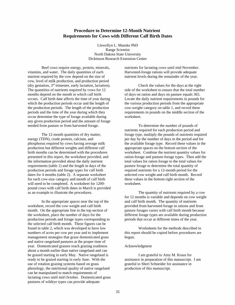
Procedure to Determine 12-Month Nutrient Requirements for Cows with Different Calf Birth Dates



Beef cows require energy, protein, minerals,vitamins, and water. The daily quantities of eachnutrient required by the cow depend on the size ofcow, level of milk production, and production period(dry gestation, 3rd trimester, early lactation, lactation). The quantities of nutrients required by cows for 12months depend on the month in which calf birthoccurs. Calf birth date affects the time of year duringwhich the production periods occur and the length ofthe production periods. The length of the productionperiods and the time of the year during which theyoccur determine the type of forage available duringany given production period and the amount of forageneeded from pasture or from harvested forage.

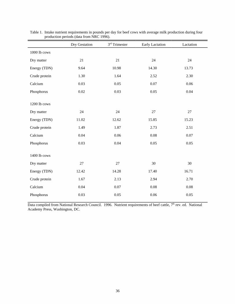
The 12-month quantities of dry matter,energy (TDN), crude protein, calcium, andphosphorus required by cows having average milkproduction but different weights and different calfbirth months can be determined with the procedurespresented in this report, the worksheet provided, andthe information provided about the daily nutrientrequirements (table 1) and the length in days of theproduction periods and forage types for calf birthdates for 4 months (table 2). A separate worksheetfor each cow-size category and month of calf birthwill need to be completed. A worksheet for 1200-pound cows with calf birth dates in March is providedas an example to illustrate the procedures.

In the appropriate spaces near the top of theworksheet, record the cow weight and calf birthmonth. On the appropriate line in the top section ofthe worksheet, place the number of days for theproduction periods and forage types corresponding tothe selected calf birth month. These figures can befound in table 2, which was developed to have lownumbers of acres per cow per year and to implementmanagement strategies that graze domesticated grassand native rangeland pastures at the proper time ofyear. Domesticated grasses reach grazing readinessabout a month earlier than native rangeland and canbe grazed starting in early May. Native rangeland isready to be grazed starting in early June. With theuse of rotation grazing systems based on grassphenology, the nutritional quality of native rangelandcan be manipulated to match requirements oflactating cows until mid October. Domesticated grasspastures of wildrye types can provide adequate

nutrients for lactating cows until mid November. Harvested-forage rations will provide adequatenutrient levels during the remainder of the year.

Check the values for the days at the rightside of the worksheet to ensure that the total numberof days on ration and days on pasture equals 365. Locate the daily nutrient requirements in pounds forthe various production periods from the appropriatecow-weight category on table 1, and record theserequirements in pounds on the middle section of theworksheet.

To determine the number of pounds ofnutrients required for each production period andforage type, multiply the pounds of nutrients requiredper day by the number of days in the period and forthe available forage type. Record these values in theappropriate spaces on the bottom section of theworksheet. Combine the nutrient quantity values forration-forage and pasture-forage types. Then add thetotal values for ration forage to the total values forpasture forage to determine the total quantity ofrequired nutrients for a 12-month period for theselected cow weight and calf birth month. Recordthese values in the bottom right section of theworksheet.

The quantity of nutrients required by a cowfor 12 months is variable and depends on cow weightand calf birth month. The quantity of nutrientsprovided from harvested forage in rations and frompasture forages varies with calf birth month becausedifferent forage types are available during productionperiods that occur at different times of the year.

Worksheets for the methods described inthis report should be copied before procedures arebegun.

Acknowledgment


36

Table 1. Intake nutrient requirements in pounds per day for beef cows with average milk production during four production periods (data from NRC 1996).

Dry Gestation 3rd Trimester Early Lactation Lactation

1000 lb cows

Dry matter 21 21 24 24

Energy (TDN) 9.64 10.98 14.30 13.73

Crude protein 1.30 1.64 2.52 2.30

Calcium 0.03 0.05 0.07 0.06

Phosphorus 0.02 0.03 0.05 0.04

1200 lb cows


Energy (TDN) 11.02 12.62 15.85 15.23

Crude protein 1.49 1.87 2.73 2.51

Calcium 0.04 0.06 0.08 0.07

Phosphorus 0.03 0.04 0.05 0.05

1400 lb cows


Energy (TDN) 12.42 14.28 17.40 16.71

Crude protein 1.67 2.13 2.94 2.70

Calcium 0.04 0.07 0.08 0.08

Phosphorus 0.03 0.05 0.06 0.05

Data compiled from National Research Council. 1996. Nutrient requirements of beef cattle, 7th rev. ed. NationalAcademy Press, Washington, DC.

Table 2. Twelve-month range cow production period sequences for calf birth dates in January to April.12-Months Calf Birth Month

January February March April

late Nov RATION RATION RATION(cont') Dry Gestation

Dec 3rd Trimester 1.0m, 32d3.0m, 90d 3rd Trimester Dry Gestation

3.0m, 90d RATION 2.0m, 62d Jan

Calf Birth 3rd Trimester3.0m, 90d

Feb Early Lactation 3rd Trimester1.0m, 32d Calf Birth 3.0m, 90d

Mar Lactation Early Lactation2.5m, 75d 1.0m, 32d Calf Birth

Apr Lactation Early Lactation1.5m, 45d 1.5m, 45d Calf Birth

Early Lactation May 0.5m, 15d

PASTURE PASTURE PASTURE PASTURELactation (spring) Lactation (spring) Lactation (spring) Lactation (spring)

Jun 1.0m, 31d 1.0m, 31d 1.0m, 31d 1.0m, 31d

JulLactation (summer) Lactation (summer) Lactation (summer) Lactation (summer)

4.5m, 137d 4.5m, 137d 4.5m, 137d 4.5m, 137d Aug

Sep

Oct Calf age-9mCalf Weaning

RATION Lactation (fall) Lactation (fall) Lactation (fall) early Nov 1.0m, 30d 1.0m, 30d 1.0m, 30d

3rd Trimester Calf age-9m Calf age-8m Calf age-7m3.0m, 90d Calf Weaning Calf Weaning Calf Weaning

Worksheet to determine 12-month nutrient requirements for cows of different sizes and with different calf birth dates.

Cow size (weight) 1200 lbs

Calf birth month March

Production Periods Dry Gestation 3rd Trimester Early Lactation Lactation

Forage Type Ration Pasture Ration Pasture Ration Pasture Ration Pasture # Days Ration

# DaysPasture

# Days12 months

Number Days from table 2 32 90 45 198 135 230 365

Requirements lbs/day from table 1.


Energy (TDN) 11.02 12.62 15.85 15.23

Crude Protein 1.49 1.87 2.73 2.51

Calcium 0.04 0.06 0.08 0.07

Phosphorus 0.03 0.04 0.05 0.05

Nutrient lbs/day X #days = Nutrient lbs/period

Totals for periods Totals forRation

Totals forPasture

Totals for 12 months

Dry matter 768 2160 1215 5346 3375 6114 9489

Energy (TDN) 352.64 1135.80 713.25 3015.54 1849.05 3368.18 5217.23

Crude Protein 47.68 168.30 122.85 496.98 291.15 544.66 835.80

Calcium 1.28 5.40 3.60 13.86 9.00 15.14 24.14

Phosphorus 0.96 3.60 2.25 9.90 5.85 10.86 16.71

Worksheet to determine 12-month nutrient requirements for cows of different sizes and with different calf birth dates.

Cow size (weight)

Calf birth month

Production Periods Dry Gestation 3rd Trimester Early Lactation Lactation

Forage Type Ration Pasture Ration Pasture Ration Pasture Ration Pasture # Days Ration

# DaysPasture

# Days12 months

Number Days fromtable 2

Requirements lbs/day from table 1.

Dry matter

Energy (TDN)

Crude Protein

Calcium

Phosphorus

Nutrient lbs/day X #days = Nutrient lbs/period

Totals for periods Totals forRation

Totals forPasture

Totals for 12 months

Dry matter

Energy (TDN)

Crude Protein

Calcium

Phosphorus

40

Reducing Beef Production Costs by Reducing Nutrient Costs



A major concern for the beef productionindustry in the Northern Plains is low profit margin. A major increase in prices appears unlikely becausecompetition from poultry and hogs is not diminishingand consumer demand for beef is weak. The beefproduction industry requires true reductions in coststo remain competitive. Beef production is the lastremaining meat industry to seriously evaluate inputcosts as a system. The future of the beef productionindustry depends on the development of long-termwhole-farm management systems that are biologicallyefficient and ecologically and economically sound.

Annual forage costs, which include the costsof pasture and harvested feed, are the major expensefor a cow-calf operation, and feed costs represent themajor expense of adding weight to growing calvesfrom weaning to finish. Traditionally, beef producershave based evaluation of production costs on the rentvalue per acre for pasture and the market value perton for harvested forages. These market values donot determine the profit or loss from forages. Theprofitability for forages can be accurately determinedfrom the costs and returns per unit of nutrientconsumed, and total profits from forages and beefanimals can be determined from the quantities ofnutrients required daily by the livestock. Thenutrients beef animals require are energy, protein,minerals, vitamins, and water.

Most beef producers in the Northern Plainshave not determined their unit costs of nutrients. Unitcosts of required nutrients must be determined toallow evaluation of production costs and identifymanagement practices that can be modified to reduceinput costs. Determining the unit cost of the requirednutrients is important to reducing production costs.

Crude protein will be used in the followingexamples to illustrate the method of calculating unitcosts of nutrients derived from purchased andharvested forage. Two values are needed todetermine costs per pound of protein for harvestedforages: the cost of the bulk forage per ton and thepercentage of crude protein contained in the forage.

Example #1

Purchased crested wheatgrass hay has avalue of $30.00 per 1000 lb bale, or $60.00per ton. The crude protein content of foragetested from this hayfield is 6.0%.

The quantity of crude protein (CP) in poundsper ton can be determined by the followingprocedure.

2000 lbs (one ton) x 6.0% = 120 lbs CP/ton

The cost per pound of crude protein can bedetermined by the following procedure.

$60.00 per ton ÷ 120 lbs CP = $0.50/lb ofCP

Example #2

Purchased alfalfa hay has a value of $120.00per ton. The crude protein content of haytested from this truckload is 18.0%.

The quantity of crude protein in pounds perton can be determined by the followingprocedure.

2000 lbs (one ton) x 18.0% = 360 lbs CP/ton

The cost per pound of crude protein can bedetermined by the following procedure.

$120.00 per ton ÷ 360 lbs CP = $0.33/lb ofCP

Management decisions based on the bulkcost of harvested forage will be different frommanagement decisions based on per unit of nutrientcosts. An illustration of the potential for reduction ofproduction costs by prudent selection and carefullytimed use of forage types at different stages of theyear can be made with 3 types of hay used for feedfor a 1200 lb cow during the 3rd trimester. A 1200 lbcow in the 3rd trimester requires 24 lbs dry matter(DM) per day at 7.8% crude protein (CP) (1.9 lbsCP/day). The standard cost rates used were tame-hayland rent at $14.22/acre and cropland rent at$22.07/acre. The standard custom farm work rates

41

were $16.08/acre and production of round bales at$5.36 per 1000 lb bale.

Crested wheatgrass cut at a mature plantstage and having the average dry matter yield of 1600lbs/acre and 6.4% CP (102 lbs CP/acre) would cost$34.80 per ton of dry matter and $0.28 per pound ofcrude protein. This late-cut hay would need to be fedat 24.0 lbs DM/day to provide 1.5 lbs CP/day. Thiscrested wheatgrass forage would cost $0.52 per day,or $46.80 for the 90-day period of the 3rd trimester. Production of this amount of crested wheatgrass haywould require 1.35 acres. An additional 0.33 lbs ofcrude protein per day would need to be provided, at acost of $9.02 per period. Total forage andsupplement costs would be $55.82 per period, or$0.62 per day.

Crested wheatgrass cut early, at the bootstage, and having the average dry matter yield of1300 lbs DM/acre and 14.5% CP (189 lbs CP/acre)would cost $40.80 per ton of dry matter and $0.14 perpound of crude protein. This early cut hay would befed at 12.9 lbs DM/day to provide 1.9 lbs CP/day. This crested wheatgrass forage would cost $0.26 perday, or $23.40 for the 90-day period of the 3rd

trimester. Production of this amount of crestedwheatgrass hay would require 0.89 acres. Anadditional 11.1 lbs of roughage per day would need tobe provided, at a cost of $17.48 per period. Totalforage and supplement costs would be $40.88 perperiod, or $0.45 per day.

Forage barley that has seed costs of $4.69per acre, is cut at the milk stage, and has the averagedry matter yield of 4733 lbs DM/acre and 13.0% CP

(606 lbs CP/acre) would cost $28.80 per ton of drymatter and $0.11 per pound of crude protein. Theforage barley hay would be fed at 14.4 lbs DM/day toprovide 1.9 lbs CP/day. This forage barley haywould cost $0.21 per day, or $18.90 for the 90-dayperiod of the 3rd trimester. Production of this amountof forage barley hay would require 0.27 acres. Anadditional 9.6 lbs of roughage per day would need tobe provided, at a cost of $14.96 per period. Totalforage and supplement costs would be $33.86 perperiod, or $0.38 per day.

These simple illustrations show that whenthe amount of crude protein harvested per acreincreases and standard costs remain constant, the costper pound of crude protein decreases, the land areaneeded for forage production per animal decreases,and the cost of feed for an animal during a productionperiod is reduced. The cost per pound of crudeprotein is a reliable indicator of relative forage costs. The cost per ton of dry matter for the forage types isnot a very reliable indicator of the actual feed costs. Improvements in harvest efficiency of the nutrientsproduced on a land base will reduce the costs per unitof nutrient and the size of the land area needed forforage production per animal and offer considerableopportunity for reductions in beef production costs.

Acknowledgment


42

Implementing Biologically Effective Grazing Management



Management of grasslands for a “use”,whether for livestock forage, wildlife habitat, oraesthetics, is management of the use, notmanagement of the grassland resources. The typicalgrassland management for a use is not sustainable ona long-term basis. Plant-friendly grasslandmanagement that meets the biological requirementsof the plants and facilitates ecological processesenhances the grassland ecosystem as a naturalresource for numerous simultaneous uses. A healthygrassland ecosystem managed by biologicallyeffective practices produces more livestock forage,better wildlife habitat, and inspirational beauty. Thesame results cannot be achieved through practicesbased on management-for-a-use concepts.

Three biologically effective managementpractices that benefit the grassland resources andimprove plant health are recommended:

• Begin grazing in the spring only after plantshave reached the third-leaf stage (early Mayfor crested wheatgrass and smoothbromegrass and early June for nativerangeland).

• Coordinate grazing rotation dates with grassgrowth stages. Plant density increases whensecondary tiller growth is stimulated bygrazing for 7 to 17 days during the periodbetween the third-leaf and flowering growthstages (early June to mid July for nativerangeland).

• Do not graze spring and summer pastures orhaylands during the fall. Fall grazingdecreases the carryover secondary tillers andthe new fall growth tillers and reduces theamount of herbage biomass produced thefollowing season.

Implementation of biologically effectivegrazing management strategies that meet thebiological requirements of the plants, enhance planthealth status, and facilitate the operation of ecologicalprocesses is the long-term solution to management-caused herbage reduction problems. The result ofthese management effects is sustained highperformance levels of healthy grassland ecosystems.

The twice-over rotation system is abiologically effective grazing management strategydeveloped for use in the Northern Plains. It was

designed to manipulate processes that result inbeneficial changes to plant growth, soil organisms,and biogeochemical cycles in the ecosystem. Thetwice-over rotation system on native rangeland withcomplementary domesticated grass spring and fallpastures coordinates defoliation with grassphenological growth stages to enhance vegetation,livestock, and wildlife performance.

The twice-over rotation system beginsgrazing in May, on a spring pasture of crestedwheatgrass or other early growing domesticated cool-season grass that has reached the third-leaf stage, theearliest plant-growth stage at which grasses can begrazed without damage. Native grasses beginseasonal development more slowly, and the use ofdomesticated grass pastures in May protects nativepastures by delaying grazing on them until the plantshave reached the third-leaf stage.

A 3- to 6-pasture native range rotationsystem is used from early June until mid October,with each pasture grazed for two periods. Eachnative rangeland pasture is grazed for 7 to 17 daysduring the first period, the 45-day interval from 1June to 15 July. The number of days each pasture isgrazed during the first period is the same percentageof 45 days as the percentage of the total season’sgrazeable forage each pasture contributes.

During the first period, grasses are betweenthe third-leaf stage and flowering phenophase. Grazing that removes a small amount of leaf areafrom grasses between these stages of plantdevelopment stimulates both tillering from axillarybuds and enhanced activity of rhizosphere organisms. Increased vegetative reproduction by tilleringcontributes to the production of greater herbageweight and nutrient quality, and increased activity ofthe symbiotic soil organisms supplies the plants withgreater quantities of nutrients to support additionalgrass tiller growth. During the second period, aftermid July and before mid October, each pasture isgrazed for double the number of days it was grazedduring the first period. Increasing the number ofsecondary tillers improves herbage quality andextends the period of improved livestock performancetwo to two and a half months, until late September ormid October. The biology of native grass plants doesnot permit extending these conditions beyond mid

43

October, when native rangeland herbage quality isinsufficient to meet the nutritional requirements oflactating cows.

Cows and calves graze a fall pasture of Altaiwildrye or other type of wildrye from mid Octoberuntil weaning in early or mid November. Wildryesare the only perennial grasses that retain nutrientquality in the aboveground portions of the plant laterthan mid October. Removing livestock from nativerangeland pastures at the end of the perennial-plantgrowing season allows native grasses to conservestored nutrients that will maintain plant processesover the winter and early spring and to retain the leafarea of secondary tillers and the fall vegetativegrowth that will become next season’s lead tillers. This practice ensures healthy plants in the spring andgreater herbage production during the followinggrowing season.

The twice-over rotation system’s elevationof plant health and stimulation of beneficialecosystem processes result in increased plant basalcover and aboveground herbage biomass andimproved nutritional quality of forage. The twice-over rotation grazing management system withcomplementary domesticated grass pastures has agrazing season of more than 6.5 months, with theavailable herbage above, at, or only slightly belowthe nutritional requirements for a lactating cow forthe entire grazing season.

The increase in quantity and quality ofherbage on the twice-over rotation system permits anincrease in stocking rate levels; improves individualanimal performance; increases total accumulatedweight gain, weight gain per acre, and weight gain

per day; reduces acreage required to carry a cow-calfpair for the season; improves net return per cow-calfpair; and improves net return per acre. The increasein basal cover and herbage biomass reduces thenumber and size of bare soil areas and increases thequantity of residual vegetation. These changes invegetation produce conditions favorable to thelimitation of grasshopper pestiferous speciespopulations. The increase in plant density, herbageproduction, residual vegetation, and ecosystem healthimproves the habitat for prairie grouse, ducks, andother waterfowl and ground nesting birds.

Effective management practices meet thebiological requirements of the plants and help theecosystem processes function at their full potential. These management practices improve theperformance levels of all grassland ecosystemcomponents, elevate plant health status, and increaseproductivity of grassland ecosystems. The result issustained greater herbage weight production, higherquality habitat for wildlife, and stronger livestockweight gain performance.

The benefits of biologically effectivegrazing practices are both ecological and economic. By implementing the twice-over rotation grazingmanagement strategy, producers protect rangelandhealth, increase their profits, and help to ensure thatthe grassland will sustain their cow-calf operation foryears to come.

Acknowledgment

I am grateful to Sheri Schneider forassistance in production of this manuscript. I amgrateful to Amy M. Kraus for assistance inpreparation of this manuscript.

44

Grassland Ecosystem Monitoring: A Nonquantitative Procedure for Assessing Rangeland Performance Status



Introduction

Sustaining rangelands at high performancelevels requires implementation of long-termmanagement practices that beneficially manipulateplant biological mechanisms and ecological processesenabling the grassland ecosystem to perform at itspeak potential. The response of biologicalmechanisms and ecological processes tomodifications of manipulation strategies is slow, andthe response of grassland ecosystem performance tomanagement practices occurs in annual incrementalchanges, both positive and negative, which may beevident only through annual monitoring. Changes inthe performance levels of several components of therangeland ecosystem can be monitored over time toprovide indirect indication of the status of grasslandecosystem health. Such monitoring allowsmanagement practices to be adjusted before problemslead to a grassland ecosystem with deteriorated healthstatus and low performance that can be improvedonly through many years of corrective manipulation.

Management practices that focus on meetingthe biological requirements of plants and facilitate theoperation of ecological processes can sustain ahealthy grassland ecosystem over time. Theperformance levels of the plant component of agrassland ecosystem regulate the performance levelsof all the other components of the ecosystem. Plantsare the primary producers, converting light energyinto chemical energy during photosynthesis. Thiscaptured solar energy is the primary force driving allecosystem functions and provides the foundation forall uses of grasslands. By meeting the biologicalrequirements of the plants and facilitating theoperation of ecological processes at potential levels,proper management practices improve theperformance of all grassland ecosystem componentsor maintain the health status and productivity of agrassland ecosystem functioning at high performancelevels. The most important components of grasslandecosystems are the plants, and they should have thehighest priority in management decisions.Management practices that focus on a single use, anidealistic goal, or an objective that does not place plant biological requirements as the first prioritycannot sustain a healthy ecosystem over time.

Rangeland health can be evaluated onlyindirectly, and its complete assessment requiresmeasurement of many complex interactivecomponents of the ecosystem. Interpretation ofecosystem performance and ecological processesrequires professional analysis of quantitativescientific data, and accurate application ofquantitative scientific methods used to measureecosystem components such as plant speciescomposition, aboveground and belowground biomassproduction, available soil water, and soil organismactivity requires professional training. Thesemethods are expensive, complex, and timeconsuming. Simple and inexpensive methods thatprovide reliable quantitative informationdocumenting the changes in rangeland ecosystemhealth have not been developed: scientific methodsmust be followed if data of scientific quality isdesired. However, rapid and inexpensive proceduresthat provide nonquantitative information can be usedto assess and monitor some changes in rangelandhealth. Nonquantitative monitoring methods need notbe executed with the precision of scientific methodsbut do require the use of valid standard procedureseach year to allow accurate comparison of thecollected information.

This report describes a simplenonquantitative grassland ecosystem monitoringmethod with three sections: plot photographs, majorplant species present list, and rangeland health statusassessment. Testing and development of monitoringprocedures were conducted during the periodbetween 1991 and 1999. Portions of this monitoringmethod are modified portions of monitoring methodsreported by Taylor and Lacey (1992) and the NationalResearch Council (1994). The nonquantitativeinformation collected by the relatively inexpensiveand easily mastered procedures presented in thisreport does not constitute an adequate substitute forscientific data and has only limited application, butthis nonquantitative information is sufficient to allowbasic evaluation of management-practiceeffectiveness.

Monitoring Site Location

Selection of appropriate monitoringlocations is necessary for accurate assessment of

45

changes that occur in ecosystem performance as aresult of the effects of management practices. Themost basic monitoring approach requires that aminimum of one site representative of the area beestablished in each pasture of a management practice.This primary monitoring site should be located on anarea that has silty soil and is relatively level: silty soilrepresents the standard soil development of a region,and the available soil water on this site type is equalto the potential amount that could be gained fromprecipitation. This monitoring site should not belocated near a gate, water tank, or road, nor should itbe located in other areas where factors in addition toenvironment or management practice might influenceecosystem response. While establishment of one siteper pasture allows basic assessment of theeffectiveness of management practices, thedevelopment of more than one site is advantageous.The number of monitoring sites per pasture shouldreflect the number of substantial land areas that havedifferences great enough to affect managementdecisions.

Traditional concepts of range conditionevaluation suggest that a monitoring site should beestablished for each range site in a pasture. Therange site, or ecological site, is the basic unit ofrangeland with similar characteristics. Each namedrange site has similar soil characteristics, topographicposition, environmental conditions, and native plantcomposition. Classification and identification ofrange sites for a grassland unit are complex processesand require the use of soil survey maps, soil seriesdescriptions, soil map unit descriptions, range sitedescriptions, and field information for specific sites.A monitoring approach using sites that represent themajor identified range sites in each pasture wouldprovide considerably more information than isessential for the formulation of most managementdecisions.

Some landscape positions vary sufficientlyin their characteristics that the differences warrantconsideration in management decisions, however. Toallow consideration of these variations, a simplifiedclassification method can be used to separate thelandscape into a few categories with differentproductivity capabilities. Landscape areas can besorted by soil parent material and average annualprecipitation into physiographic regions. The landwithin these physiographic regions can then beclassified into three general landscape site categoriesbased on whether the amount of soil water is greaterthan, equal to, or less than the potential amount thatcould be gained from precipitation. The threecategories are lowland, upland, and xeric sites.Lowland landscape sites have high levels of soil

water in the rooting zone for most of the year.Because of water run-in, the water levels in thesesites are greater than precipitation levels. Theamount of water run-in is variable with landscapeposition. Depressions or basins on lower portions ofslopes receive greater amounts of run-in water thanconcave portions of side slopes. Upland landscapesites have well-drained soils and are usually not atfield capacity for much of the growing season. Theamount of soil water in these sites usually reflects thepotential amount that could be gained fromprecipitation. The primary monitoring site located onsilty soil is an upland landscape site. Xeric landscapesites have restricted infiltration or water-holdingcapacity, and, for most of the growing season,available soil water is below the levels that could begained from precipitation. The dryness of xeric sitesusually results from the physical characteristics of thesite rather than from lack of precipitation. Thelandscape of management-practice pastures can beclassified into these three general landscape typecategories, and a monitoring site for each landscapetype present in each pasture can be established todifferentiate variations in productivity that are greatenough to affect management decisions. Thismonitoring approach provides useful information andis strongly recommended.

Additional monitoring sites may bedesignated to document the health status of thepasture more thoroughly. In pastures that containplant communities at different levels of health,selection of monitoring sites representative of thedifferent levels is suggested to facilitate evaluation ofthe communities’ response to management practices.Location of other sites in areas of particular concernmay be useful to monitor the response of special plantcommunities to the effects of management practices.

Inclusion of a monitoring site in controlareas of long-term (seven or more years) nongrazingand/or six-month seasonlong grazing treatment isrecommended. Monitoring sites in control areasshould be located on the same types of range sites orlandscape sites selected in the management-practicepastures. Comparison of changes observed on themanagement-practice pastures to changes observedon control areas can help distinguish changes causedby the management practice from changes caused byvariability in environmental factors.

Monitoring Site Description

A description of each monitoring site shouldbe prepared at the start of the monitoring process.Forms on which to record pertinent informationfollow the text of this report. Each monitoring site

46

description should include pasture name or number,legal description, soil type, range site or landscapesite, physical characteristics, implementedmanagement practices, and weather conditions. Therecord of physical characteristics should includetopography, percent slope, and aspect (exposure). Amap of the monitoring sites should be made anddirections enabling someone not familiar with theoperation to locate each monitoring site should beprovided. The description of pasture managementpractices should be completed annually and shoulddocument type of grazing management, pasture sizein acres, number and type of livestock, and dates ofgrazing periods. A general description of each year’sprevailing weather conditions should also beprovided. Descriptions should be organized bymonitoring site and placed in a three-ring binder orother type of orderly filing system.

Photo Plot Method

Photographs taken at designated monitoringsites can reveal a considerable amount of informationabout changes in a rangeland ecosystem whenstandard procedures are followed for several years.To depict the current characteristics of the ecosystem,a vertical and a horizontal photograph should betaken for each monitoring plot during each samplingperiod. Monitoring site photographs can aid in theevaluation process and serve as documentation for theresults of the pasture’s health status assessment.

The needed materials are a camera, film, aplot frame, a portable elevated photo platform, plotand date information tags, pins, posts, and a photoalbum. The same camera and film type should beused for all plot photographs. A plot frame withinside dimensions of a square yard or square meter isused to demarcate the plot boundaries in thephotographs. The photo plot frame should be painteda bright color or with alternated stripes of knownlength. A portable elevated platform is needed toprovide enough vertical distance between the cameraand the plot that the entire plot frame will be capturedin the photograph. People of average height require aplatform elevated 18" to 24". The distance betweencamera and plot should be constant among all verticalphotographs, so it is desirable that photographs betaken by persons who are of similar height and whouse the same portable platform. A plastic 5-gallonrestaurant pickle bucket serves as an inexpensiveportable elevated platform that can also be used tocarry equipment between sites. A modestly pricedthree-step stool can serve as a safe elevated platformif balancing on an overturned bucket seems tooreckless. Plot tags, which bear the identifying nameor number assigned the monitoring plot to be

photographed, and date identification tags, whichrecord the exact date of the plot photograph, can bemade from cardboard shipping tags. The lettering onthe tags should be large and dark enough to be readeasily on the photographs. The identification tag anddate tag should be placed just outside the plot framewhen the photograph is taken and can be held inplace with large nails.

Each photo plot requires four pins to markthe corners permanently and two steel posts toindicate the location of the plot. Inexpensive pins canbe made from large washers welded ontoreinforcement rod. One pin should be driven into thesoil at each corner of the plot, and the tops of thewashers should be painted a bright color. A locationpost should be set at a known distance and in aknown direction from the plot, and a sight post shouldbe set further away, in line with the location post andthe center of the plot. All photo monitoring plotsshould follow the same master plan: for example, asteel location post might be set 50 feet north of thecenter of the photo plot and a sight post 20 to 30 feetpast the location post to assist in the relocation of theplot. A rope with a loop on one end and with thesame length as the distance between the location postand the plot center can be used to assist in therelocation of a plot when the photographer places theloop over the location post and walks in an arc at theend of the outstretched rope.

The greater the number of sampling periodsat which photographs are taken at each monitoringsite, the more thoroughly the conditions will berepresented. A minimum of three photo samplingperiods per site per year is necessary to depict annualseasonal changes. The first photo should be taken inearly June, when plants are at the grazing-readystage. The second should be taken when peakherbage biomass has been produced, usually betweenmid July and the first week in August. The thirdshould be taken during the late portion of the growingseason, sometime between mid and late September,when the status of cool-season fall-tiller growth isevident. If grazing continues in one or two pasturesafter mid October, a fourth photo should be taken inthese pastures at the end of grazing, even if snowcovers the ground.

Photographs should be taken during thesame periods each year. The vertical photographsshould be taken with the photographer alwayspositioned on the same side of the plot, preferably onthe north so that his or her shadow is not cast on thephoto plot. The camera should be elevated the samedistance above the plot for each photograph, and thesame platform should be used each time. Sharp focus

47

on the photo plot is critical, and the focus should bechecked through the viewfinder of the camera whilethe photograph is taken.

After the vertical photograph for eachsampling period has been taken, a horizontalphotograph across the plot should be taken from apoint 15 feet from the plot and opposite the locationpost; the horizontal photograph should be taken fromthe same spot each time. For this shot, the plot frameshould be positioned upright to give perspective tothe plot. The plot frame will stand in an uprightposition if one side is supported by a rod struck intothe soil.

Monitoring site photographs should beorganized by year and preserved in a photo album orbinder. Photographic negatives should be storedseparately in case damage to the photographs occurs.

Major Plant Species Present List

Major plant species composition on amonitoring site undergoes dynamic changes. Plantspecies composition changes both in response toenvironmental factors such as precipitation levels andpattern, hail, drought, and abnormal hot or coldperiods and in response to defoliation managementpractices of grazing and fire. The effects of fire orgrazing vary with time of season, frequency, andseverity of defoliation. Percent composition ofindividual plant species may increase or decreaseunder one set of conditions and reverse that responseunder another set of conditions. To help documentthe dynamic changes in plant species compositionthat occur over time, a list of major plant species

present on each monitoring site should be made onceeach year, between mid July and mid August. Duringthis period most plants will be at an identifiable stage,including plants with their primary growth occurringduring the early or late portions of the growingseason. The major plant species, including grasses,forbs, and shrubs, should be listed from most to leastdominant. The minor plant species may be recordedbut need not be. The book Range Plants, written byK.K. Sedivec and W. T. Barker and published byNDSU in 1997, can aid in proper identification ofspecies. The major plant species present list willassist in the evaluation of the monitoring site and inthe identification of plants observed in the monitoringsite photographs. The list will also serve asdocumentation for the rangeland health assessment.

Each rangeland plant species grows bestwithin a suite of environmental parameters. Plantspecies with similar requirements generally growtogether on landscape positions that have similarphysical and environmental conditions. Landscapepositions with different physical and environmentalconditions support plant communities with differentmajor plant species composition. Landscapepositions can be classified into three generallandscape sites that have different physical andenvironmental conditions. The major grass speciespresent on lowland, upland, and xeric landscape sitesare listed in tables 1, 2, and 3, respectively. Not allspecies listed in each table will be found on allrespective landscape sites. The groupings of grassspecies in these tables may assist in the identificationof the three general landscape sites on the pasturelandscape and can be used as a reference guide duringthe recording of the major plant species present list. The plant list for each site should be placed in thethree-ring binder with the descriptions of themonitoring site and management practices.

48

Table 1. Major grasses of the lowland and saline lowland landscape sites.



Big bluestem Andropogon gerardi

Northern reedgrass Calamagrostis stricta

Canada wildrye Elymus canadensis

Switchgrass Panicum virgatum

Reed canarygrass Phalarisarundinacea

Sprangletop Scolochloafestucacea

Indiangrass Sorghastrum nutans

Prairie cordgrass Spartina pectinata

Slough sedge Carex atherodes

Wooly sedge Carex lanuginosa

Lowland sedges Carex spp.

Saline Lowland Landscape Sites

Inland saltgrass Distichlis spicata

Foxtail barley Hordeum jubatum

Nuttall alkaligrass Puccinellianuttalliana

Tumblegrass Schedonnarduspaniculatus

Squirreltail Sitanion hystrix

Alkali cordgrass Spartina gracilis

Table 2. Major grasses of the upland landscape sites.



Sand bluestem Andropogon hallii

Sideoats grama Boutelouacurtipendula


Plains reedgrass Calamagrostismontanensis

Prairie sandreed Calamovilfa longifolia


Little bluestem Schizachyriumscoparium

Sand dropseed Sporoboluscryptandrus


Porcupine grass Stipa spartea



Table 3. Major grasses of the xeric landscape sites.




Buffalograss Buchloe dactyloides


Plains muhly Muhlenbergiacuspidata

Sandberg bluegrass Poa sandbergii

Little bluestem Schizachyriumscoparium




49

Nonquantitative Assessment of Rangeland HealthStatus

Assessment of rangeland health status isdifferent from the traditional method fordetermination of range condition, which compares thecurrent successional stage of the plant community tothe theoretical climax plant community. Rangelandhealth assessment evaluates both the performancelevels at which ecosystem components arefunctioning and the interactions among climate, soil,vegetation, and animals. Rangeland health is not aphysical characteristic of the ecosystem, and thestatus of health can be assessed only indirectly,through evaluation of the levels of performance ofmany ecosystem components. The ecosystemcomponents considered during health statusassessment procedures are aboveground andbelowground vegetation, soil development processes,levels and types of erosion, ecological processes, andprecipitation infiltration.

Most rangeland health status assessmentmethods separate the relative rankings of theperformance and health of rangeland ecosystems intofour condition categories, from extremely healthy toextremely unhealthy. The most commonly usedcondition category names are excellent, good, fair,and poor. In the nonquantitative rangeland healthstatus assessment method presented, these fourgeneral categories will be used to separate the levelsof ecosystem health. Evaluation criteria andcharacteristics of the major components vary indegree and functional status for the four rangelandhealth condition categories.

The four rangeland health conditioncategories can be illustrated by comparison to humanhealth condition. A grassland ecosystem in excellent(A) condition is like a highly trained athlete: highlyproductive, with all processes functioning at highrates and high efficiency; able to endure considerable

stress; and capable of rebounding from stress quickly. A grassland ecosystem in good (B) condition is like aperson in average health: productive, with allprocesses functioning at moderate rates and moderateefficiency; able to endure some stress; and capable ofgradual recovery from stress. A grassland ecosystemin fair (C) condition is like a couch potato: marginallyproductive, with all processes functioning at low ratesand reduced efficiency; able to endure only minimalstress; and requiring long periods to recover fromstress. A grassland ecosystem in poor (D) conditionis like a chronically ill person: unproductive, with allprocesses functioning ineffectively and inefficiently;unable to endure stress; and capable of recoveringfrom stress only over considerable time and withspecial treatment.

Assessment of the status of rangelandecosystem health should be conducted for eachmonitoring site each year, between early June andlate July. The evaluation criteria and characteristicsfor excellent (A), good (B), fair (C), and poor (D)rangeland health condition categories are on tables 4,5, 6, and 7, respectively. All seventeen health statuscriteria and characteristics should be assessed for themonitoring site, and the ecosystem’s condition foreach characteristic should be placed at one of the fourlevels though determination of whether the grasslandecosystem performs like a highly trained athlete (A),a person in average health (B), a couch potato (C), ora chronically ill person (D). A set of questions to helpthe evaluator interpret the seventeen health statuscriteria and characteristics is provided.

A form on which ten years of assessmentsmay be recorded is located at the end of this report.The health status assessment form for each siteshould be placed in the three-ring binder with the sitedescriptions and the major plant species present lists.

50

The following set of questions can be used to help interpret the rangeland health status criteria andcharacteristics on tables 4-7 and to help place the grassland ecosystem into a health condition category.

I. What is the density of the plants? Are they close together with few open spaces, or are numerous large openspaces evident?

II. What is the plant species composition? Are most of the plants desirable prairie species, or are mostundesirable species?

III. What are the age groups of the plants? Are there numerous young plants, or are there very few young plants?

IV. How vigorous are the plants? Are the plants large and robust, or are they weak?

V. What is the root distribution in the soil? Are roots growing throughout the soil profile, or are roots restrictedto a small portion of the soil profile?

VI. What is the quantity of leaf material present throughout the growing season? Are substantial quantities ofgrass leaves present at the end of the season, or are the grass leaves grazed short during any portion of theseason?

VII. How much litter is present? Does litter cover the entire area, or is litter present only in small amounts anddistributed only in small patches?

VIII. What is the distribution of decomposed organic matter? Is the organic matter spread over the entire area, or isit present only in small patches?

IX. What is the distribution of developing soil? Is the soil top layer dark and continuous, or is it light colored?

X. What is the extent of erosion? Is very little soil moved by wind or water, or is a considerable amount of soilmoved?

XI. What is the extent of soil deposition? Are small or large quantities of recently deposited soil present?

XII. What is the extent of recent gully formation? Are the gullies relatively shallow and gently sloping, or are theydeep and branching?

XIII. What is the extent of pedestaling? Is pedestaling absent, or are roots exposed on some pedestals?

XIV. What is the extent to which wind erosion and water erosion are changing the surface? Are there areas that arepolished clean, or are there areas that have windrows of plant material near the base of a hill after a rainstorm?

XV. The nutrient cycles and energy flow cannot be directly observed, but the presence of dark soil and healthydesirable plants with robust leaves and roots indicates adequate energy flow and function of nutrient cycles.

XVI. The dynamics and processes of an ecosystem cannot be directly observed, but the presence of dark soil andhealthy desirable plants with robust leaves and roots indicates healthy ecosystem dynamics and processes.

XVII. What is the level of precipitation infiltration? Does most of the rain soak into the soil, or does a significantamount run off?

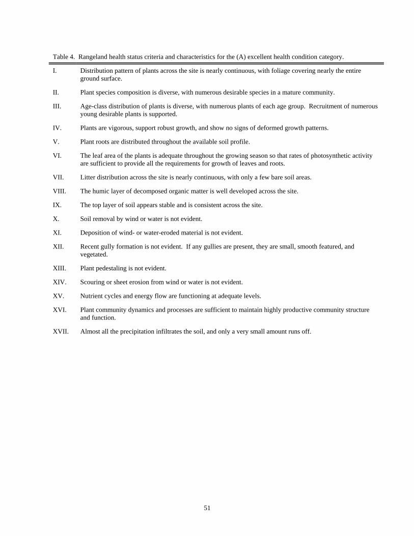
51

Table 4. Rangeland health status criteria and characteristics for the (A) excellent health condition category.

I. Distribution pattern of plants across the site is nearly continuous, with foliage covering nearly the entireground surface.

II. Plant species composition is diverse, with numerous desirable species in a mature community.

III. Age-class distribution of plants is diverse, with numerous plants of each age group. Recruitment of numerousyoung desirable plants is supported.

IV. Plants are vigorous, support robust growth, and show no signs of deformed growth patterns.

V. Plant roots are distributed throughout the available soil profile.

VI. The leaf area of the plants is adequate throughout the growing season so that rates of photosynthetic activityare sufficient to provide all the requirements for growth of leaves and roots.

VII. Litter distribution across the site is nearly continuous, with only a few bare soil areas.

VIII. The humic layer of decomposed organic matter is well developed across the site.

IX. The top layer of soil appears stable and is consistent across the site.

X. Soil removal by wind or water is not evident.

XI. Deposition of wind- or water-eroded material is not evident.

XII. Recent gully formation is not evident. If any gullies are present, they are small, smooth featured, andvegetated.

XIII. Plant pedestaling is not evident.

XIV. Scouring or sheet erosion from wind or water is not evident.

XV. Nutrient cycles and energy flow are functioning at adequate levels.

XVI. Plant community dynamics and processes are sufficient to maintain highly productive community structureand function.

XVII. Almost all the precipitation infiltrates the soil, and only a very small amount runs off.

52

Table 5. Rangeland health status criteria and characteristics for the (B) good health condition category.

I. Distribution pattern of plants across the site is somewhat continuous, with foliage covering almost all theground surface.

II. Plant species composition is diverse, with numerous desirable species and a few less desirable species in amature community.

III. Age-class distribution of plants is diverse, with many plants of each age group. Recruitment of many youngdesirable plants is supported.

IV. Plants are vigorous and show no signs of deformed growth patterns.

V. Plant roots are distributed throughout nearly all the available soil profile.

VI. The leaf area of the plants is adequate throughout the growing season so that rates of photosynthetic activityare sufficient to provide nearly all the requirements for growth of leaves and roots.

VII. Litter distribution across the site is somewhat continuous, with only a small amount of bare soil area.

VIII. The humic layer of decomposed organic matter is present over most of the site.

IX. The top layer of soil appears stable and nearly uniform across the site.

X. Soil removal by wind or water shows very little evidence.

XI. Deposition of wind- or water-eroded material shows very little evidence.

XII. Recent gully formation shows very little evidence. If some gullies are present, they are smooth featured andvegetated.

XIII. Plant pedestaling shows little evidence.

XIV. Scouring or sheet erosion from wind or water shows very little evidence.

XV. Nutrient cycles and energy flow are functioning at adequate levels.

XVI. Plant community dynamics and processes are sufficient to maintain the existing community structure andfunction.

XVII. Most of the precipitation infiltrates the soil, and only a small amount runs off.

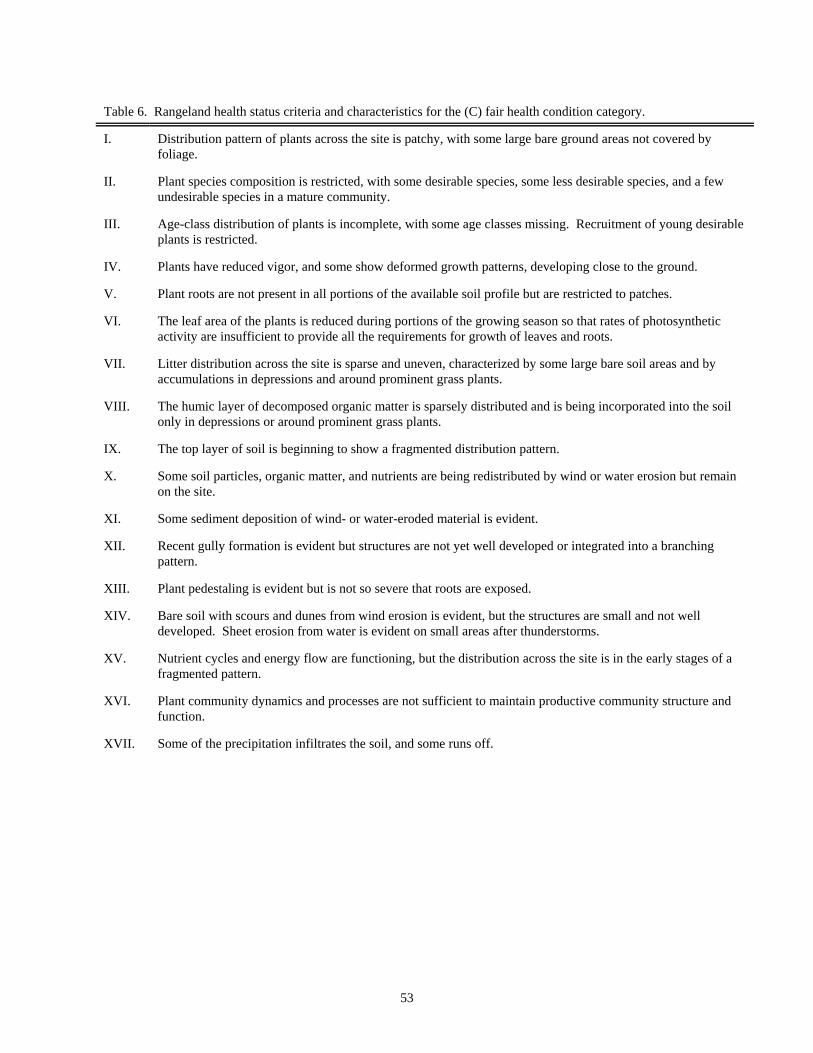
53

Table 6. Rangeland health status criteria and characteristics for the (C) fair health condition category.

I. Distribution pattern of plants across the site is patchy, with some large bare ground areas not covered byfoliage.

II. Plant species composition is restricted, with some desirable species, some less desirable species, and a fewundesirable species in a mature community.

III. Age-class distribution of plants is incomplete, with some age classes missing. Recruitment of young desirableplants is restricted.

IV. Plants have reduced vigor, and some show deformed growth patterns, developing close to the ground.

V. Plant roots are not present in all portions of the available soil profile but are restricted to patches.

VI. The leaf area of the plants is reduced during portions of the growing season so that rates of photosyntheticactivity are insufficient to provide all the requirements for growth of leaves and roots.

VII. Litter distribution across the site is sparse and uneven, characterized by some large bare soil areas and byaccumulations in depressions and around prominent grass plants.

VIII. The humic layer of decomposed organic matter is sparsely distributed and is being incorporated into the soilonly in depressions or around prominent grass plants.

IX. The top layer of soil is beginning to show a fragmented distribution pattern.

X. Some soil particles, organic matter, and nutrients are being redistributed by wind or water erosion but remainon the site.

XI. Some sediment deposition of wind- or water-eroded material is evident.

XII. Recent gully formation is evident but structures are not yet well developed or integrated into a branchingpattern.

XIII. Plant pedestaling is evident but is not so severe that roots are exposed.

XIV. Bare soil with scours and dunes from wind erosion is evident, but the structures are small and not welldeveloped. Sheet erosion from water is evident on small areas after thunderstorms.

XV. Nutrient cycles and energy flow are functioning, but the distribution across the site is in the early stages of afragmented pattern.

XVI. Plant community dynamics and processes are not sufficient to maintain productive community structure andfunction.

XVII. Some of the precipitation infiltrates the soil, and some runs off.

54

Table 7. Rangeland health status criteria and characteristics for the (D) poor health condition category.

I. Distribution pattern of plants across the site is clumped or fragmented, with numerous large bare ground areasnot covered by foliage.

II. Plant species composition is restricted, with few desirable species, many less desirable species, and manyundesirable species in a developing community.

III. Age-class distribution of plants is restricted, with predominantly old or deteriorated plants. Recruitment ofyoung desirable plants is nearly absent.

IV. Plants are weak, and many plants show deformed growth patterns, developing close to the ground.

V. Plant roots occupy only a small portion of the available soil profile.

VI. The leaf area of the plants is greatly reduced during portions of the growing season so that photosyntheticactivity is restricted to rates too low to provide much of the energy or many of the nutrients required forgrowth of leaves and roots.

VII. Litter distribution across the site is sparse or absent, with numerous large bare soil areas.

VIII. The humic layer of decomposed organic matter is sparse or absent from most of the site.

IX. The top layer of soil is sparse or absent from large areas of the site or is present only in association withdepressions or prominent obstructions.

X. Soil degradation resulting from soil particle, organic matter, and nutrient removal from the site by wind orwater is evident.

XI. Deposition of wind- or water-eroded material is evident, appearing as large bare deposits, as dunes, or inassociation with prominent plants.

XII. Recent gully formation is evident, and structures are well developed, active, and integrated into a branchingpattern.

XIII. Plant pedestaling is severe enough that roots are exposed.

XIV. Bare soil with scours and dunes from wind erosion is evident. The structures are active and well developed. Sheet erosion from water is evident on large areas after thunderstorms.

XV. Nutrient cycles and energy flow are decelerated, and the distribution pattern is fragmented, with numerouslarge bare areas between fragments.

XVI. Plant community dynamics and processes are not sufficient to maintain viable community structure andfunction.

XVII. Only a small amount of the precipitation infiltrates the soil, and most runs off.

55

Interpretation

The Grassland Ecosystem Monitoring(GEM) procedures can be mastered easily and can beimplemented and conducted effectively by grasslandmanagers who have received training in thefundamentals of the method. The informationcollected with this three-part grassland ecosystemmonitoring procedure is adequate to allow basicevaluation of the effectiveness of managementpractices. Current year’s photographs, major plantsspecies list, and nonquantitative assessment ofrangeland health status for each monitoring siteshould be compared to previous years’ records for thesite. The interpretation of observed changes will beaided by reference to the rangeland health statuscriteria and characteristics in tables 4 to 7. Changeson the management-practice monitoring sites shouldalso be compared to changes on control-treatmentareas of long-term nongrazing and/or six-monthseasonlong grazing so that changes caused by theeffect of the management practice can bedistinguished from changes caused by variability inenvironmental factors. An annual narrativedescription of the observed changes in the photographs, plant list, and ecosystem healthassessment information should be completed for eachmonitoring site.

Changes in the status of the grasslandecosystem performance will be positive or negative.Evaluation of the collected material will allowmanagers to follow incremental improvement inperformance or to make adjustments to managementpractices before problems lead to deterioration of theecosystem health status. When the grasslandecosystems are performing at potential levels, thismonitoring procedure will provide documentationthat management practices meet the biologicalrequirements of the plants and facilitate ecologicalprocesses.

Worksheets for the methods described inthis report should be copied before procedures arebegun. Additional worksheets are available on theweb at http://www.ag.ndsu.edu/dickinso/research/2001/range01j.htm.

Acknowledgment

I am grateful to Amy M. Kraus forassistance in the preparation of this manuscript. I amgrateful to Sheri Schneider for assistance inproduction of this manuscript and for development ofthe tables and forms.

References

Manske, L.L. 1999. Generalized range sites groupcategories. NDSU Dickinson ResearchExtension Center. Range ProgramInformation Sheet #7. Dickinson, NorthDakota. 6p.

Manske, L.L. 1999. Simplified method forassessment of range condition. NDSUDickinson Research Extension Center. RangeProgram Information Sheet #8. Dickinson,North Dakota. 7p.

Manske, L.L. 1999. Historical steps in thedevelopment of the concept of rangecondition. NDSU Dickinson ResearchExtension Center. Range ProgramInformation Sheet #11. Dickinson, NorthDakota. 2p.

National Research Council. 1994. Rangelandhealth: New methods to classify, inventory,and monitor rangelands. National AcademyPress, Washington, DC.

Sedivec, K.K., and W.T. Barker. 1997. SelectedNorth Dakota and Minnesota range plants. NDSU Extension Service. EB-69. Fargo,North Dakota. 270p.

Taylor, J.E., and J. Lacey. 1992. MonitoringMontana rangeland. MSU Extension Service. Bulletin 369. Bozeman, Montana. 22p.

56

Monitoring Procedure Time Table

Photo Plot Method

Minimum of 3 photo periods per year: information collected from permanent photo plot

1st early June grazing-ready stage

2nd mid July to early August peak herbage biomass

3rd mid to late September fall tiller growth

4th pastures grazed after midOctober

end of grazing

Major Plant Species Present List

Once a year: information collected from permanent photo plot

mid July to mid August plants identifiable

Nonquantitative Assessment of Rangeland Health Status

Once a year: information collected from vicinity of permanent photo plot

early June to late July characteristicsobservable

57

Description of Monitoring Site

Monitoring Site Name: _____________________________________________________________________

Pasture Name: ____________________________________________________________________________

Physical Characteristics

Range Site or Landscape Site: __________________________________________________________

Soil Type (sand, silt, clay): _____________________________________________________________

Topography: ________________________________________________________________________

Percent Slope (rise/distance): ___________________________________________________________

Aspect (compass direction of slope): _____________________________________________________

Legal Description (quarter, quarter, quarter section): ______________________________________________

Location Description: ______________________________________________________________________

___________________________________________________________________________________

___________________________________________________________________________________

Direction and Distance of Location Post from Photo Plot Center: ____________________________________

Photo Plot Frame Size: ______________________________________________________________________

Attach a map of the location of the monitoring sites.

Provide directions that someone not familiar with the operation could follow to reach this monitoring site.

58

Annual Description of Management Practices

Monitoring Site Name: _____________________________________________________________________

Pasture Name: ____________________________________________________________________________

Year: ____________________________________________________________________________________

Grazing Practice Size in Acres: _______________________________________________________________

Pasture Size in Acres: ______________________________________________________________________

Type of Livestock: _________________________________________________________________________

Number of Livestock: ______________________________________________________________________

Dates of Grazing Periods: ___________________________________________________________________

____________________________________________________________________________________

Description of Grazing Management Practices: __________________________________________________

____________________________________________________________________________________

____________________________________________________________________________________

____________________________________________________________________________________

____________________________________________________________________________________

____________________________________________________________________________________

General Description of Weather Conditions

Previous Fall: _____________________________________________________________________________

Previous Winter: __________________________________________________________________________

Before 1st Photo Period: _____________________________________________________________________

Before 2nd Photo Period: ____________________________________________________________________

Before 3rd Photo Period: _____________________________________________________________________

____________________________________________________________________

59

Rangeland Ecosystem Health Status Assessment

Monitoring Site Name:

Range Site or Landscape Site:

Health Condition Categories

Trained Athlete (A) Excellent Average Person (B) Good Couch Potato (C) Fair Chronically Ill (D) Poor

Evaluation Number

1 2 3 4 5 6 7 8 9 10

Day

Month

Year

I. Plant distribution

II. Plant species diversity

III. Plant age class

IV. Plant vigor

V. Plant root distribution

VI. Amount of leaf area remaining

VII. Litter distribution

VIII. Humic layer development

IX. Soil development processes

X. Extent of soil erosion

XI. Extent of soil deposition

XII. Extent of gully development

XIII. Plant pedestaling

XIV. Erosional changes of soil surface

XV. Ecological processes

XVI. Ecosystem dynamics

XVII. Precipitation infiltration

Name of Evaluator

methods for development of biologically effective

Documents