methodologies for u.s. greenhouse gas emissions
TRANSCRIPT

Methodologies for U.S. Greenhouse Gas
Emissions Projections:
Non-CO2 and Non-Energy CO2 Sources
DECEMBER, 2013
U.S. Environmental Protection Agency
1200 Pennsylvania Ave., N.W.
Washington, DC 20460
U.S.A.

i
Preface
This report was prepared by the U.S. Environmental Protection Agency (EPA) with the support of its
contractors, ERG and Ricardo-AEA. This report describes the methodology used by EPA to project
emissions of greenhouse gas (GHG) emissions other than combustion-related carbon dioxide (CO2) out
to the year 2030 in a range of source categories. The sources of U.S. non-CO2 GHG and non-energy CO2
emissions are in the energy; industrial processes; solvent and product use; waste; agriculture; and land
use, land-use change, and forestry sectors.
In May through July of 2013, the draft final report was peer reviewed for its technical content by: Mr.
Shankar Ananthakrishna of Chevron; Dr. Morton A. Barlaz of North Carolina State University; Mr. E. Lee
Bray of the U.S. Geological Survey; Mr. Stuart Day of Australia’ Commonwealth Scientific and Industrial
Research Organisation; Mr. Jon Elliott of the United Kingdom Department of Energy and Climate
Change; Ms. Céline Gueguen of the Interprofessional Technical Centre for Studies on Air Pollution
(CITEPA); Dr. Lena Höglund-Isaksson of the International Institute for Applied Systems Analysis; Dr.
Lambert Kuijpers of the Technical University Eindhoven and a member of the Montreal Protocol’s
Technology and Economic Assessment Panel; Dr. Peter Lahm of the U.S. Forest Service; Dr. Sim Larkin of
the U.S. Forest Service; Dr. Jan Lewandrowski of the U.S. Department of Agriculture; Dr. Gregg Marland
of Appalachian State University; Mr. Etienne Mathias of CITEPA; Dr. David McCabe of the Clean Air Task
Force; Dr. John Reilly of the Massachusetts Institute of Technology; Mr. Lukas Rothlisberger of the DILO
Company; Mr. Bruce Steiner of the American Coke and Coal Chemicals Institute; Mr. Hendrik G. van Oss
of the U.S. Geological Survey; Mr. Julien Vincent of CITEPA; and Ms. Lynn Yeung of the California Air
Resources Board. The peer reviewers were asked to draw upon their expertise in non-CO2 and non-
energy CO2 sectors and source categories, as well as in GHG emission projection methods, to comment
on whether the data inputs, approach, and methodologies presented in the report reflect sound
scientific and analytical practice, and adequately address the questions at hand.
Written comments were received from the peer reviewers. The reviewers generally commented that the
methodologies used in this report represented a sound approach to projecting U.S. non-CO2 GHG and
non-energy CO2 emissions. A number of comments identified areas for technical clarification, alternative
datasets, and opportunities for future improvements. All comments of the reviewers were considered,
and the document was modified appropriately.
EPA wishes to acknowledge everyone involved in the development of this report, and to thank the peer
reviewers for their time, effort, and expert guidance. The involvement of the peer reviewers greatly
enhanced the technical soundness of this report. EPA accepts responsibility for all information
presented and any errors contained in this document.
Climate Change Division
Office of Atmospheric Programs
U.S. Environmental Protection Agency
Washington, DC 20460

Methodologies for U.S. GHG Projections: Non-CO2 and Non-Energy CO2 Sources ii
Contents Preface ................................................................................................................................... i
1.0 Introduction ............................................................................................................... 1
1.1 Background ...................................................................................................................................... 1
1.2 Sectors and Key Category Analysis .................................................................................................. 1
1.3 General Approach ............................................................................................................................ 3
Activity Drivers .......................................................................................................................... 3
Scenarios ................................................................................................................................... 3
Policies and Measures ............................................................................................................... 4
Technology Characterization and Change ................................................................................. 5
1.4 Quality Assurance and Quality Control ............................................................................................ 5
1.5 Uncertainty ...................................................................................................................................... 6
1.6 Equations ......................................................................................................................................... 7
2.0 Source Methodologies ................................................................................................ 8
2.1 Energy .............................................................................................................................................. 8
Stationary Source Combustion .................................................................................................. 8
Mobile Source Combustion ..................................................................................................... 11
Non-Energy Uses of Fossil Fuels .............................................................................................. 12
Coal Mining .............................................................................................................................. 14
Natural Gas Systems ................................................................................................................ 17
Petroleum Systems .................................................................................................................. 29
2.2 Industrial Processes ....................................................................................................................... 32
Cement Production ................................................................................................................. 32
Adipic Acid Production ............................................................................................................ 35
Iron and Steel Production and Metallurgical Coke Production ............................................... 37
Aluminum Production ............................................................................................................. 38
Magnesium Production and Processing .................................................................................. 40
HCFC-22 Production ................................................................................................................ 41
Substitution of Ozone-Depleting Substances .......................................................................... 44
Semiconductor Manufacturing ............................................................................................... 46

Methodologies for U.S. GHG Projections: Non-CO2 and Non-Energy CO2 Sources iii
Electrical Transmission and Distribution ................................................................................. 49
2.3 Agriculture ..................................................................................................................................... 51
Enteric Fermentation .............................................................................................................. 51
Manure Management ............................................................................................................. 54
Rice Cultivation ........................................................................................................................ 56
Agricultural Soil Management ................................................................................................. 58
2.4 Land Use, Land-Use Change, and Forestry .................................................................................... 62
CH4 and N2O Emissions from Forest Fires ............................................................................... 62
2.5 Waste ............................................................................................................................................. 65
Landfills .................................................................................................................................... 65
Domestic Wastewater Treatment ........................................................................................... 68
3.0 References ............................................................................................................... 74

Methodologies for U.S. GHG Projections: Non-CO2 and Non-Energy CO2 Sources 1
1.0 Introduction
This report presents the methodology used by the U.S. Environmental Protection Agency (EPA) to
estimate projections of greenhouse gas (GHG) emissions other than combustion-related carbon dioxide
(CO2) out to the year 2030. The sources of U.S. non-CO2 GHG and non-energy CO2 emissions are in the
energy; industrial processes; solvent and product use; waste; agriculture; and land use, land-use change,
and forestry sectors. This report describes the specific methods used to project emissions for each
source category. EPA will generate the projections by applying this methodology within a data system
designed specifically to project the non-CO2 GHG emissions.
1.1 Background
The U.S. government provides projections of U.S. GHG emissions for international reporting purposes as
part of U.S. Climate Action Reports (CARs) to the United Nations Framework Convention on Climate
Change (UNFCCC). EPA has coordinated the production of these projections, which are assembled from
projections produced by the U.S. Department of Energy’s (DOE’s) Energy Information Administration
(EIA), the U.S. Department of Agriculture (USDA), and EPA. EPA is responsible for estimating projections
for the non-CO2 GHG and non-energy CO2 sources.
New international reporting requirements for biennial reports now require updates to the U.S. GHG
emissions projections every two years, instead of every four years as in the past.
1.2 Sectors and Key Category Analysis
Table 1 lists the sectors and source categories that generate non-CO2 GHG and non-energy CO2
emissions. The sector list is based on the source categories characterized in the U.S. GHG Inventory.
Because of the large number of sources, EPA developed source-specific projection methodologies for a
limited set of source categories. The remaining categories use a generic projection methodology. Two
criteria have been used to designate the sources for which specific projection methodologies were
developed:
1. All source categories designated as “key categories” in the 2012 U.S. GHG Inventory
2. Additional source categories of special interest, such as due to the presence of mitigation programs
This document focuses on describing the source-specific methodologies used to project emissions. The
generic projection approach used for other sources was to extrapolate emissions based on the historical
trend over the previous 10 years. For sources where emissions increased over that time period, a linear
extrapolation was used; for declining emissions, an exponential extrapolation was used. EPA used these
different approaches to contain projections within reasonable bounds over the long projection time
period (i.e., growth tends to come up against physical limitations and decline should not go below zero
emissions).

Methodologies for U.S. GHG Projections: Non-CO2 and Non-Energy CO2 Sources 2
Table 1. Non-CO2 and Non-Energy CO2 Projection Source Categories
Check Mark () Indicates That Source-Specific Methodologies Were Developed
Sector Source(s) Key Categories Non-Key Categories
Energy
Coal mining CH4
Stationary combustion sources CH4, N2O
Natural gas systems CH4, non-energy CO2
Petroleum systems CH4
Non-energy use of fuels Non-energy CO2
Abandoned underground coal mines CH4
Mobile combustion CH4, N2O
International bunker fuels CH4, N2O
Incineration of waste N2O, non-energy CO2
Industrial Processes
Adipic acid production N2O
Substitution of ozone-depleting substances HFCs
HCFC-22 production HFCs
Aluminum production PFCs, non-energy CO2
Electric transmission and distribution SF6
Cement production Non-energy CO2
Iron and steel production and metallurgical coke production
Non-energy CO2 CH4
Magnesium production SF6
Nitric acid production N2O
Silicon carbide production CH4, non-energy CO2
Ferroalloy production CH4, non-energy CO2
Semiconductor manufacturing HFCs, PFCs, SF6
Lime production Non-energy CO2
Limestone and dolomite use Non-energy CO2
Ammonia production Non-energy CO2
Urea consumption for non-agricultural purposes
Non-energy CO2
Soda ash production and consumption Non-energy CO2
Petrochemical production CH4, non-energy CO2
Carbon dioxide consumption Non-energy CO2
Titanium dioxide production Non-energy CO2
Zinc production Non-energy CO2
Phosphoric acid production Non-energy CO2
Lead production Non-energy CO2
Agriculture
Enteric fermentation CH4
Agricultural soil management N2O
Rice cultivation CH4 N2O
Manure management CH4 N2O
Field burning of agricultural residues CH4, N2O
Waste
Landfills CH4
Wastewater treatment (domestic) CH4, N2O
Wastewater treatment (industrial) CH4
Composting CH4, N2O
Solvent and Product Use
N2O product usage N2O
Land Use, Land-Use Change, and
Forestry
Forest fires (forest land remaining forest land) CH4, N2O
Wetlands remaining wetlands N2O, non-energy CO2
Cropland remaining cropland Non-energy CO2
Settlements remaining settlements N2O

Methodologies for U.S. GHG Projections: Non-CO2 and Non-Energy CO2 Sources 3
1.3 General Approach
The basic approach used to project these emissions was based on using inventory methodologies to
estimate emissions in future years. EPA used information from the most recent U.S. GHG Inventory (EPA
2013) as the starting point for emissions and underlying activities. EPA projected changes in activity data
and emissions factors from that base year. For the current projections, EPA used the year 2011 for the
base year, drawn from the 2013 U.S. GHG Inventory. Activity data projections include macroeconomic
drivers such as population, gross domestic product, and energy use, and source-specific activity data
such as fossil fuel production, industrial production, or livestock populations and crop production.
Future changes in emissions factors were based on continuation of past trends and expected changes
based on implementation of policies and measures.
Key elements of the overall methodology are summarized below.
Activity Drivers
Unlike emissions inventories developed for past or present inventory years—which are typically based
upon actual measured or quantified activity data statistics—future year projections have no activity data
available, by definition. Instead, activity drivers are used to estimate future year activity levels.
Activity drivers serve as proxies, allowing the development of reasonable approximations of future year
activity from base year activity levels. For instance, the U.S. Census Bureau and other agencies have
developed reasonably accurate long-term population projections, based on past trends and a general
understanding of long-term demographic behavior. These long-term population projections can be used
to develop future year activity level estimates for source categories that use population-based activity
data (e.g., domestic wastewater treatment, landfills). Another example is the long-term energy
production and consumption projections developed by EIA in conjunction with the Annual Energy
Outlook. These energy projections are developed using a sophisticated model that seeks to accurately
represent all aspects of U.S. energy; they can be used to develop future year activity level estimates for
source categories that use energy-based activity data (e.g., non-energy uses of fossil fuels, natural gas
systems, petroleum systems). Additional source-specific activity drivers are discussed below in Section
2.0.
Scenarios
The methodologies discussed in this document describe a projection scenario including the effects of
currently implemented policies and measures, referred to in the UNFCCC context as a “with measures”
scenario. This type of scenario is also sometimes referred to as a reference, baseline, or business-as-
usual scenario, although the term “business-as-usual” can also refer to a scenario not including the
effects of policies. Within the international reporting context, countries are also encouraged to provide
a “without measures” scenario removing the effect of policies and measures, and an “additional
measures” scenario including planned policies and measures. These two alternative scenario types are
not addressed in this document.
Methodologies for U.S. GHG Projections: Non-CO2 and Non-Energy CO2 Sources 4
The “with measures” scenario uses a central estimate for various activity drivers. Although the results of
applying these methodologies will be a single projection estimate, there is uncertainty in each element
of the projections. In some cases, activity driver projections provide low and high scenarios that could
be used to develop low and high sensitivity projection scenarios in the future.
Policies and Measures
The projection methodologies for each source include the effects of currently implemented policies and
measures (PAMs). Policies implemented after the production of projections would not be included
without changes to the methodology. Policies are included in various ways depending on the source.
Considered policies include both regulatory and voluntary programs, and both policies specifically aimed
at reducing GHGs, as well as policies with other main purposes that have indirect impacts on GHG
emissions.
EPA has included these effects in the projections in different ways depending on the source category
and the data available. In some cases, potential emissions are calculated based on activity data and
emissions factors, and then estimates of PAM-related reductions are used to reduce potential emissions
resulting in actual emissions. In other cases, the effects of longstanding policies and measures are
included within the calculation of aggregate emissions factors based on historical emissions and
activities. In yet other cases, estimates of reductions due to newly implemented policies and measures
are based on the specific provisions of policies. Lastly, the use of external activity data implicitly includes
the effects of policies modeled as part of those external projections. For example, EIA projections
include the effects of various energy and environmental policies in the Annual Energy Outlook
projections of fossil fuel production, so that when those projections are used to calculate fugitive
emissions, various policies are indirectly accounted for in these non-CO2 and non-energy CO2 projections.
The term “policies and measures” describes both regulatory requirements and voluntary programs.
PAMs may adjust the activity data, emissions factors, or calculated emissions. In many cases, regulatory
PAMs do not specifically target GHG emissions, but are cobenefits. Regulatory PAMs create reductions
due to mandated requirements; examples include applicable subparts of the New Source Performance
Standards (NSPS) and state-level regulations. Voluntary PAMs create reductions in response to various
incentives or motivating factors. Examples of voluntary PAMs include the Natural Gas STAR program, the
Landfill Methane Outreach Program, and incentives that promote renewable energy (e.g., tax credits,
low-interest loans, Renewable Portfolio Standards).
The implementation of PAMs throughout the projection time series must be carefully considered. Some
PAMs may simply be a certain reduction quantity or percent reduction that can be applied over the
entire time series. However, some regulatory PAMs are phased in over a number of years. One example
is a regulation that requires reductions for a certain type of equipment at some future date and

Methodologies for U.S. GHG Projections: Non-CO2 and Non-Energy CO2 Sources 5
reductions for a different type of equipment at another future date. Another example is mandatory
reductions that only apply to new equipment; over time this new equipment with reductions would be
gradually incorporated into the overall equipment population as old equipment ages and is replaced.
Technology Characterization and Change
In general, base year emissions estimates represent the current state of technology and its associated
level of implementation within each source category. However, most of the long-term non-CO2
projections do not address any potential future technological improvements in emissions control
technologies. Such improvements may occur in response to various environmental, economic, or social
drivers. Significant technological improvements will reduce actual future emissions below the projected
estimates; adjustments to the projection methodology may be required to address these technological
improvements.
1.4 Quality Assurance and Quality Control
The non-CO2 projection system has been designed around the IPCC approach to create good quality
estimates of GHG emissions. The quality system has two main components: quality control and quality
assurance. The full IPCC definitions of quality control and quality assurance are as follows:
Quality Control (QC) is a system of routine technical activities to assess and maintain the
quality of the inventory as it is being compiled. It is performed by personnel compiling the
inventory. The QC system is designed to:
(i) Provide routine and consistent checks to ensure data integrity, correctness, and
completeness;
(ii) Identify and address errors and omissions;
(iii) Document and archive inventory material and record all QC activities. QC activities
include general methods such as accuracy checks on data acquisition and calculations,
and the use of approved standardised procedures for emission and removal calculations,
measurements, estimating uncertainties, archiving information and reporting. QC
activities also include technical reviews of categories, activity data, emission factors, other
estimation parameters, and methods.
Quality Assurance (QA) is a planned system of review procedures conducted by
personnel not directly involved in the inventory compilation/development process.
Reviews, preferably by independent third parties, are performed upon a completed
inventory following the implementation of QC procedures. Reviews verify that
measurable objectives were met, ensure that the inventory represents the best possible

Methodologies for U.S. GHG Projections: Non-CO2 and Non-Energy CO2 Sources 6
estimates of emissions and removals given the current state of scientific knowledge and
data availability, and support the effectiveness of the QC programme.
Mechanisms to ensure QC are embedded in the non-CO2 projections calculations in several ways. The
source-category specific spreadsheets have been designed to be transparent, for example: calculations
flow logically from the top of the sheet to the bottom; constants appear first, then source data are
listed; all relevant cells in the workbooks are color-coded for easy reference, indicating whether the cells
provide calculations, outputs, QC checks, or data input. The calculations make extensive use of lookup
functions to ensure that consistent unit conversions are used throughout. Data validation rules and
drop-down menus for source, activity, scenario, and unit names are used to ensure that only those for
which valid lookups exist within the database can be selected. Also, a QA worksheet is contained in each
source-category specific spreadsheet that contains both automated and manual QC checks.
QA will be implemented through a process of independent review of the both the workbooks and the
methodologies used to generate the projections.
1.5 Uncertainty
Uncertainties in projections combine the uncertainties in the estimation approaches used for the base
year inventory as well as uncertainties in anticipating changes in activity data and emissions factors over
the projection period.
Uncertainties in GHG inventories arise from the estimating activity data and the emissions factors. Some
sources of emissions are inherently more uncertain than others. For example, non-CO2 emissions from
agriculture arise from natural processes and as such can be difficult to characterize. Emissions from soils
can depend on meteorology and soil type, in addition to the amount of fertilizer applied or the amount
and types of crops grown; emissions from livestock can change depending on the feed type. Emissions of
CO2 from fossil fuel combustion are much easier to estimate and are therefore less uncertain, as long as
the composition of the fuel and the amount of fuel are both well known.
The uncertainty in total GHGs in the U.S. GHG Inventory is estimated to be -2 to +5 percent in 2011, at a
95 percent confidence interval. Since total GHG emissions are dominated by CO2 from fuel combustion,
the overall uncertainty is low. However, for the non-CO2 gases, and non-energy CO2 sources, the
uncertainties are higher (e.g., +13 to -14 percent for CH4, -9 to +41 percent for N2O). The uncertainty
related to individual sources is higher still, and can vary significantly between sources. For example,
emissions from iron and steel production have relatively low uncertainty (-12 to +12 percent for CH4)
while emissions from petroleum systems have high uncertainty (-24 to +149 percent for CH4).

Methodologies for U.S. GHG Projections: Non-CO2 and Non-Energy CO2 Sources 7
Projecting GHG emissions adds another layer of uncertainty. For example, changes in industry structure
over time, the particular impacts of policies, changing weather and economic conditions all add
variability to how future emissions will develop. Some indication of the degree of uncertainty related to
projection variables can be gained by looking at the range of published scenarios for these factors. Some
source documents, such as the EIA Annual Energy Outlook, present alternative scenarios which differ
from their reference scenario regarding key variables. For example, the range between the low and high
economic growth scenarios for GDP is -8.8 and +9.4 percent relative to the reference case; for the low
and high oil and gas resource scenario natural gas production varies -13.6 to +18.1 percent.
In discussing the uncertainties for projections, it is useful to separate out the uncertainty in the GHG
projection from the uncertainty inherent in estimating historical GHG emissions. The uncertainties
related to historical inventories should be combined with the uncertainties related to projected activity
data and emissions factors to account for the full potential for uncertainty in projected emissions. A
quantitative uncertainty analysis has not been carried out for the current set of projections, but EPA
plans to more thoroughly characterize uncertainty in future versions of these projections.
1.6 Equations
Calculations for each source throughout this document use a similar template wherein source emissions
are projected by multiplying emissions factors by projected activity data. In many cases, the base year
inventory uses more detailed activity data than is available for projections, and so an aggregate
emissions factor is calculated by dividing historical emissions by historical activity data. In general there
are sometimes minor differences in scope or estimates of base year activity data between the U.S. GHG
Inventory and the data source used for projections. To ensure consistency with the historical inventory,
the projected change in the activity data from the base year is applied to the base production level
presented in the inventory.
(
)
Equation 1
Where:
Emissionsy = Projected emissions in year y EFagg = Aggregate emissions factor InventoryActivityb = Historical activity data from U.S. GHG Inventory in base year b ProjectedActivityb = Activity estimate for base year b from projection data source ProjectedActivityy = Activity data projections for year y from projection data source y = projected year b = base year

Methodologies for U.S. GHG Projections: Non-CO2 and Non-Energy CO2 Sources 8
2.0 Source Methodologies
Source-specific methodologies are presented in this section, by sector: energy; industrial processes;
agriculture; land use, land-use change, and forestry; and waste.
2.1 Energy
Stationary Source Combustion
Source Description
The direct combustion of fuels by stationary sources in the electricity generation, industrial, commercial,
and residential sectors represents the greatest share of U.S. GHG emissions. CH4 and N2O emissions
from stationary combustion sources depend on fuel characteristics, size, and vintage, along with
combustion technology, pollution control equipment, ambient environmental conditions, and operation
and maintenance practices. N2O emissions from stationary combustion are closely related to air-fuel
mixes and combustion temperatures, as well as the characteristics of any pollution control equipment
that is employed. CH4 emissions from stationary combustion are primarily a function of the CH4 content
of the fuel and combustion efficiency.
Emissions projections estimated in this section include CH4 and N2O from stationary source combustion.
Combustion also results in CO2 emissions, but those emissions are covered by energy-related CO2
emissions projections beyond the scope of this report. This source category is included within IPCC
guidelines source subcategory 1A. CO2 from non-energy use of fuels is covered in a separate projections
category, although the U.S. GHG Inventory (EPA 2013) discusses them together. Emissions from U.S.
territories are included.
Methodology
EPA calculated projected emissions from this source category by summing projections of emissions from
residential, commercial, industrial, and electric power sources. Each of these sources includes coal, fuel
oil, natural gas, and wood fuel combustion. Combustion in the U.S. territories was added separately. CH4
and N2O emissions for each category were calculated separately:
Residential o Coal o Fuel oil o Natural gas o Wood and biomass
Commercial o Coal o Fuel oil o Natural gas o Wood and biomass
Industrial o Coal

Methodologies for U.S. GHG Projections: Non-CO2 and Non-Energy CO2 Sources 9
o Fuel oil o Natural gas o Wood and biomass
Electric power o Coal o Fuel oil o Natural gas o Wood and biomass
U.S. territories o Coal o Fuel oil o Natural gas o Wood and biomass
As shown above, each sector was subdivided by fuel type, including coal, fuel oil, natural gas, and wood.
The CH4 and N2O emissions estimation methodology used in the U.S. GHG Inventory was revised in 2010
to use the facility-specific technology and fuel use data reported to EPA’s Acid Rain Program.
Residential, Commercial, and Industrial
EPA estimated projected CH4 and N2O emissions associated with stationary combustion from the
residential, commercial, and industrial sectors by multiplying consumption projections for each sector
and fuel from the U.S. Energy Information Administration, or EIA (EIA 2013)1 by the Tier 1 default
emissions factors provided by the 2006 IPCC Guidelines (IPCC 2006), which were also used to calculate
emissions in the U.S. inventory. Future wood consumption projections for commercial and industrial
sectors were not available from the EIA; therefore, historical wood consumption data (by sector) from
EIA were extrapolated (based on the annual percent change over the previous 10 years) to estimate
future consumption through the end of the projection period. EPA then multiplied wood consumption
projections by sector-specific Tier 1 default emissions factors provided by the 2006 IPCC Guidelines to
estimate future CH4 and N2O emissions.
Electric Power
To project CH4 and N2O emissions from combustion in the electric power sector, EPA multiplied (for each
fuel type) projected U.S. electricity generation by an aggregate emissions factor based on historical CH4
and N2O emissions and historical electricity generation. Projected electricity generation came from EIA’s
Annual Energy Outlook (EIA 2013). EPA calculated aggregate emissions factors for each fuel source by
dividing historical emissions from electricity generation (by fuel source) from the EPA inventory by
historical generation from EIA over the most recent five years and averaging the results. As with the
residential, commercial, and industrial sectors, future wood consumption projections for the electric
power sector were not available from the EIA; therefore, historical wood consumption data from the EIA
1 Sectoral information for U.S. territories (American Samoa, Guam, Puerto Rico, U.S. Virgin Islands, Wake Island,
and other U.S. Pacific Islands) is not available from EIA. Based on the U.S. GHG Inventory, CH4 and N2O emissions from U.S. territories are negligible; therefore, fuel consumption in U.S. territories was not included in the stationary combustion emissions projections.

Methodologies for U.S. GHG Projections: Non-CO2 and Non-Energy CO2 Sources 10
were extrapolated based on the annual percent change over the previous 10 years to estimate future
wood consumption through the end of the projection period.
The projection methodology for CH4 and N2O from electric power differs from that used in the U.S.
Inventory. The inventory uses a Tier 2 methodology for the electric power sector,2 whereas all other
sectors for stationary combustion use a Tier 1 methodology. Specifically, the Tier 2 methodology for the
electric power sector uses electric-facility-specific technology and fuel use data reported under EPA’s
Acid Rain Program.
U.S. Territories
Information on underlying combustion activity for the U.S. territories is not included in the Annual
Energy Outlook. Therefore, EPA calculated projections of CH4 and N2O emissions from combustion in the
U.S. territories by extrapolating emissions based on the annual percent change over the most recent 10
years.
2 CH4 and N2O emissions for the electric sector from previous years listed in the U.S. GHG Inventory were also
adjusted using the new Tier 2 methodology approach.
Methodologies for U.S. GHG Projections: Non-CO2 and Non-Energy CO2 Sources 11
Mobile Source Combustion
Source Description
Mobile combustion produces GHGs other than CO2, including CH4, N2O, and indirect GHGs including NOx,
CO, and NMVOCs. As with stationary combustion, N2O and NOx emissions from mobile combustion are
closely related to fuel characteristics, air-fuel mixes, combustion temperatures, and the use of pollution
control equipment. N2O from mobile sources, in particular, can be formed by the catalytic processes
used to control NOx, CO, and hydrocarbon emissions. CO emissions from mobile combustion are
significantly affected by combustion efficiency and the presence of post-combustion emissions controls.
CO emissions are highest when air-fuel mixtures have less oxygen than required for complete
combustion. These emissions occur especially in idle, low-speed, and cold start conditions. CH4 and
NMVOC emissions from motor vehicles are a function of the CH4 content of the motor fuel, the amount
of hydrocarbons passing uncombusted through the engine, and any post-combustion control of
hydrocarbon emissions (such as catalytic converters).
Emissions projections estimated in this section include CH4 and N2O from mobile source combustion.
Combustion also results in CO2 emissions, but those emissions are covered by energy-related CO2
emissions projections beyond the scope of this report. This source category is included within IPCC
guidelines source subcategory 1A.
Methodology
CH4 and N2O emissions from this source category are modeled using the Motor Vehicle Emissions
Simulator (MOVES), developed by EPA’s Office of Transportation and Air Quality.3 Results were
calculated based on runs of the MOVES2010b, the latest version of the MOVES system, using national
default inputs. The MOVES2010b model estimates the vehicle population and activity data including
miles driven and number of starts for each vehicle source type using a variety of information sources, as
documented by EPA (2010). These projected activity estimates are then multiplied by appropriate
emissions rates. N2O emissions are calculated directly, while CH4 emissions are derived from emissions
rates for total hydrocarbons. The N2O emissions rates and the CH4/THC ratios are described in EPA
(2012d).
3 MOVES2010b and related information and documentation can be found online at
<http://www.epa.gov/otaq/models/moves/index.htm>.

Methodologies for U.S. GHG Projections: Non-CO2 and Non-Energy CO2 Sources 12
Non-Energy Uses of Fossil Fuels
Source Description
In addition to being combusted for energy, fossil fuels are consumed for non-energy uses (NEUs) in the
United States. The fuels used for these purposes are diverse, including natural gas, liquefied petroleum
gases (LPG), asphalt (a viscous liquid mixture of heavy crude oil distillates), petroleum coke
(manufactured from heavy oil), and coal (metallurgical) coke (manufactured from coking coal). The non-
energy applications of these fuels are equally diverse, including feedstocks for the manufacture of
plastics, rubber, synthetic fibers and other materials; reducing agents for the production of various
metals and inorganic products; and non-energy products such as lubricants, waxes, and asphalt (IPCC
2006).
CO2 emissions arise from NEUs via several pathways. Emissions may occur during the manufacture of a
product, as is the case in producing plastics or rubber from fuel-derived feedstocks. Additionally,
emissions may occur during the product’s lifetime, such as during solvent use. Overall, throughout the
time series and across all uses, about 62 percent of the total carbon consumed for non-energy purposes
was stored in products, and not released to the atmosphere; the remaining 38 percent was emitted.
This emissions source covers CO2 emissions from NEUs of fossil fuels. This corresponds to a part of IPCC
source 1A, as described in the U.S. GHG Inventory (EPA 2013).
Methodology
EPA calculated emissions projections for this source by multiplying base year CO2 emissions from NEUs
of fossil fuels in the U.S. GHG Inventory by the growth in industrial energy consumption of feedstocks
and fuels usually used for non-energy purposes in the Annual Energy Outlook (EIA 2013). Growth in CO2
from NEUs of fuels is assumed to be proportional to the total energy content of consumed energy
(excluding refining) of LPG feedstock, petrochemical feedstocks, asphalt and road oil, and natural gas
feedstocks (see the AEO table “Industrial Sector Key Indicators and Consumption”).
Equation 2
Where:
Emissionsy = Projected emissions in year y
Emissionsb = Emissions in the base year
NEU-Energyy = NEU energy in year y
NEU-Energyb = NEU energy in the base year
Non-Energy Use of Fuels in the U.S. GHG Inventory
For background, the calculation of emissions from non-energy use of fuels in the U.S. GHG Inventory is
described here for the purpose of understanding the emissions included in the base year. In the U.S.
GHG Inventory, EPA estimated the amount of carbon stored in products to determine the aggregate

Methodologies for U.S. GHG Projections: Non-CO2 and Non-Energy CO2 Sources 13
quantity of fossil fuels consumed for NEUs. The carbon content of these feedstock fuels is equivalent to
potential emissions, or the product of consumption and the fuel-specific carbon content values. Both
the non-energy fuel consumption and carbon content data were supplied by the U.S. Energy Information
Administration (EIA 2013). Consumption of natural gas, LPG, pentanes plus, naphthas, other oils, and
special naphtha were adjusted to account for net exports of these products that are not reflected in the
raw data from EIA. For the remaining NEUs, EPA estimated the quantity of carbon stored by multiplying
the potential emissions by a storage factor.
Methodologies for U.S. GHG Projections: Non-CO2 and Non-Energy CO2 Sources 14
Coal Mining
Source Description
CH4, which is contained within coal seams and the surrounding rock strata, is released into the
atmosphere when mining operations reduce the pressure above and/or surrounding the coal bed. The
quantity of CH4 emitted from these operations is a function of two primary factors: coal rank and coal
depth. Coal rank is a measure of the carbon content of the coal, with higher coal ranks corresponding to
higher carbon content and generally higher CH4 content. Pressure increases with depth and prevents
CH4 from migrating to the surface; as a result, underground mining operations typically emit more CH4
than surface mining. In addition to emissions from underground and surface mines, post-mining
processing of coal and abandoned mines also release CH4. Post-mining emissions refer to CH4 retained in
the coal that is released during processing, storage, and transport of the coal.
This emissions source covers fugitive CH4 emissions from coal mining (including pre-mining drainage)
and post-mining activities (i.e., coal handling), including both underground and surface mining. This
corresponds to IPCC source category 1B1a, excluding emissions from abandoned underground mines
(which are included as a separate source category, corresponding to IPCC category 1B1a3).
Methodology
EPA calculated emissions projections for this source by summing emissions associated with underground
mining, post-underground mining, surface mining, and post-surface mining.
∑
Equation 3
Where:
s = Sources (underground, post-underground, surface, and post-surface mining)
Emissionsy,s = Emissions in year y from source s
EPA projected emissions from each source by multiplying an aggregate emissions factor by projected
coal production (for underground or surface mining as appropriate). Projected reductions due to
recovery and use are then subtracted from potential emissions.4
4 Current CH4 recovery and use projects apply to underground mining, but projects related to surface mining could
be implemented in the future.

Methodologies for U.S. GHG Projections: Non-CO2 and Non-Energy CO2 Sources 15
(
)
Equation 4
Where:
EFagg,s = Aggregate emissions factor associated with source s
InventoryProductionb,s = Coal production associated with source s in the base
year from the U.S. GHG Inventory5
ProjectedProductiony,s = Projected coal production associated with the emissions
source (e.g., either underground or surface mining) in year y
CH4RecoveryUseFracs = Fraction of CH4 recovered from source s
Emissions Factors
To calculate potential emissions from each category, EPA calculated an aggregate CH4 emissions factor
using historical CH4 emissions and coal production data contained in the most recent U.S. GHG Inventory
(EPA 2013). For example, , historical CH4 liberated by underground mining was divided by the total
underground coal production for the corresponding year. The aggregate emissions factor is the average
of this ratio over the most recent five years. Similar calculations were performed for post-underground
mining emissions, surface mining emissions, and post-surface mining emissions, using either historical
underground or surface mining production data as appropriate.
The projection methodology differs from the estimation methodology used in the U.S. GHG Inventory.
The inventory does not use emissions factors to calculate CH4 emissions from underground mines. The
U.S. GHG Inventory estimates total CH4 emitted from underground mines as the sum of CH4 liberated
from ventilation systems (mine-by-mine measurements) and CH4 liberated by means of degasification
systems, minus CH4 recovered and used. EPA estimated surface mining and post-mining CH4 emissions
by multiplying basin-specific coal production, obtained from EIA’s Annual Coal Report (EIA 2012), by
basin-specific emissions factors.6
Coal Production Projections
EPA projected emissions using projections of underground, surface, and total coal production from the
EIA Annual Energy Outlook (AEO) (EIA 2013). The 2013 AEO projects the total coal production for the
United States, as well as the coal production by region, and by various characteristics including
underground and surface mining (see AEO table “Coal Production by Region and Type”).
EIA provides historical regional coal production data broken out between underground and surface
mining in its Annual Coal Report (EIA 2012). EPA collated and calculated the proportion of production,
underground versus surface, for each year. (EPA determined the total underground mining coal
5 Because of slight differences between historical and projection datasets, values for production in the base year from each
dataset do not cancel

Methodologies for U.S. GHG Projections: Non-CO2 and Non-Energy CO2 Sources 16
production and the total surface mining coal production for the United States by summing the regional
totals for each year.) There has been a general trend toward increasing surface mining relative to
underground mining (EPA 2013).
CH4 Mitigation (Recovery and Use)
EPA projected coal mine CH4 mitigation by calculating the historical fraction of methane recovered in
relation to generation from underground mines, and applying that fraction to future generation. The
historical fraction was averaged over the most recent five years. Future mitigation was estimated by
applying the historical rate of recovery and use to projected potential emissions generated.
The U.S. GHG Inventory uses quantitative estimates of CH4 recovery and use from several sources.
Several gassy underground coal mines in the United States employ ventilation systems to ensure that
CH4 levels remain within safe concentrations. Additionally, some U.S. coal mines supplement ventilation
systems with degasification systems, which remove CH4 from the mine and allow the captured CH4 to be
used as an energy source.
∑
⁄
Equation 5
Where:
CH4RecoveryUses,y = Recovered emissions from source s in year y
Potential Emissionss, y = Potential emissions from source s in year y
b = base year

Methodologies for U.S. GHG Projections: Non-CO2 and Non-Energy CO2 Sources 17
Natural Gas Systems
Source Description
The U.S. natural gas system encompasses hundreds of thousands of wells, hundreds of processing
facilities, and over a million miles of transmission and distribution pipelines. CH4 and non-combustion7
CO2 emissions from natural gas systems are generally process-related, with normal operations, routine
maintenance, and system upsets being the primary contributors. There are four primary stages of the
natural gas system which are briefly described below.
Production
In this initial stage, wells are used to withdraw raw gas from underground formations. Emissions arise
from the wells themselves, gathering pipelines, and well-site gas treatment facilities (e.g., dehydrators,
separators). Major emissions source categories within the production stage include pneumatic devices,
gas wells with liquids unloading, and gas well completions and re-completions (i.e., workovers) with
hydraulic fracturing (EPA 2013). Flaring emissions account for the majority of the non-combustion CO2
emissions within the production stage.
Processing
In this stage, natural gas liquids and various other constituents from the raw gas are removed, resulting
in “pipeline-quality” gas, which is then injected into the transmission system. Fugitive CH4 emissions
from compressors, including compressor seals, are the primary emissions source from this stage. The
majority of non-combustion CO2 emissions in the processing stage come from acid gas removal units,
which are designed to remove CO2 from natural gas.
Transmission and Storage
Natural gas transmission involves high-pressure, large-diameter pipelines that transport gas long
distances from field production and processing areas to distribution systems or large-volume customers
such as power plants or chemical plants. Compressor station facilities, which contain large reciprocating
and turbine compressors, are used to move the gas throughout the U.S. transmission system. Fugitive
CH4 emissions from these compressor stations and from metering and regulating stations account for
the majority of the emissions from this stage. Pneumatic devices and uncombusted engine exhaust are
also sources of CH4 emissions from transmission facilities. Natural gas is also injected and stored in
underground formations, or liquefied and stored in above-ground tanks, during periods of lower
demand (e.g., summer), and withdrawn, processed, and distributed during periods of higher demand
(e.g., winter). Compressors and dehydrators are the primary contributors to emissions from these
storage facilities. Emissions from LNG import terminals are included within the transportation and
storage stage.
7 In this document, consistent with IPCC accounting terminology, the term “combustion emissions” refers to the
emissions associated with the combustion of fuel for useful heat and work, while “non-combustion emissions” refers to emissions resulting from other activities, including flaring and CO2 removed from raw natural gas.

Methodologies for U.S. GHG Projections: Non-CO2 and Non-Energy CO2 Sources 18
Distribution
Distribution pipelines take the high-pressure gas from the transmission system at “city gate” stations,
reduce the pressure, and then distribute the gas through primarily underground mains and service lines
to individual end users.
Coverage
Projections for this source cover CH4 and non-combustion CO2 emissions from natural gas systems.
Combustion CO2 emissions are covered by energy-related CO2 emissions projections outside the scope
of this report. The corresponding source for natural gas systems in the 2006 IPCC guidelines is 1B2b.
Methodology
The methodology for natural gas emissions projections involves the calculation of CH4 and CO2 emissions
for over 100 emissions source categories across the four natural gas sector stages, and then the
summation of emissions for each sector stage. The calculation of emissions for each source of emissions
in natural gas systems generally occurs in three steps:
1. Calculate potential CH4
2. Estimate reductions data associated with voluntary action and regulations
3. Calculate net emissions
EPA calculated potential CH4 emissions from natural gas systems by summing the projections associated
with (1) production, (2) processing, (3) transmission and storage, and (4) distribution. In general, activity
data were projections of natural gas production and consumption from the Energy Information
Administration, or EIA (EIA 2013). Additional activity data for projections included liquefied natural gas
(LNG) imports, pipeline length, and number of service lines. Because the base year inventory emissions
explicitly include reductions due to voluntary and regulatory requirements, the projections also include
appropriate explicit mitigation projections as well. Emissions for each source were estimated using the
following equation:
Equation 6
Where:
NEs,y = Projected net emissions for source s in year y
PEs,y = Projected potential emissions for source s in year y
VRs,y = Projected voluntary reductions for source s in year y
RRs,y = Projected regulatory reductions for source s in year y
The sections below describe detailed calculations for projections of CH4 from natural gas systems. Non-
combustion CO2 emissions also result from natural gas systems, mainly from the production and
processing stages. In the production stage, non-combustion CO2 mostly results from flaring. In the
processing stage, non-combustion CO2 comes mostly from acid gas removal units, which are designed to
remove CO2 from natural gas. EPA calculated projected non-combustion CO2 emissions from the
Methodologies for U.S. GHG Projections: Non-CO2 and Non-Energy CO2 Sources 19
production and processing stages by scaling emissions in the base year by the increase in projected
natural gas production in the Annual Energy Outlook (AEO) (EIA 2013).
Production Stage
The production stage includes a total of 35 emissions source categories. Regional emissions were
estimated in the base year inventory for the six supply regions (i.e., Northeast, Gulf Coast, Midcontinent,
Southwest, Rocky Mountain, and West Coast) for 33 of these sources.
Potential Emissions
EPA estimated future year potential emissions for the production stage using the following equation.
(
)
Equation 7
Where:
PEs,y = Projected future potential emissions for source s in year y
PEs,b = Estimated potential emissions for source s in base year b
Gas Productiony = Projected natural gas dry production year y
Gas Productionb = Estimated natural gas dry production for base year b
The natural gas dry production estimates were obtained from the Annual Energy Outlook (AEO)
Supplemental Tables published by EIA.8
Voluntary Reductions
Projections of voluntary reductions for the production stage were based on historical data reported by
industry to the Natural Gas STAR program for projects implemented to reduce emissions. Natural Gas
STAR tracks projects on an annual basis and assigns a lifetime of limited duration to each reduction
project; for purposes of the base year emissions inventory and the future year projections, the
reductions associated with each project were either considered to be a “one-year” project or a
“permanent” project based on sunset dates provided by the Natural Gas STAR program. Reductions
from “one-year” projects were typically from the implementation of new or modified practices, while
reductions from “permanent” projects tended to be from equipment installation, replacement, or
modification. In the base year emissions inventory and the future year projections, reductions for a
“one-year” project were limited to the project’s reported start year, while reductions for a “permanent”
project were assigned to the project’s reported start year and every subsequent year thereafter. Thus,
the reductions due to “permanent” projects gradually accumulated throughout the inventory time
series, while the reductions due to “one-year” projects were replaced every year.
The following production stage voluntary reductions were reported to Natural Gas STAR and applied to
individual sources in the emissions inventory:
8 References to the AEO Supplemental Tables in this methodology do not indicate year or table number because
these will change every year.
Methodologies for U.S. GHG Projections: Non-CO2 and Non-Energy CO2 Sources 20
Completions for gas wells with hydraulic fracturing (one year)—perform reduced emissions
completions (RECs).
Pneumatic device vents (one year)—reduce gas pressure on pneumatic devices; capture/use gas
released from gas-operated pneumatic pumps.
Pneumatic device vents (permanent)—identify and replace high-bleed pneumatic devices; convert
pneumatic devices to mechanical controls; convert to instrument air systems; install no-bleed
controllers.
Kimray pumps (permanent)—install/convert gas-driven pumps to electric, mechanical, or solar
pumps.
Gas engines compressor exhaust (one year)—replace ignition/reduce false starts; turbine fuel use
optimization.
Gas engines compressor exhaust (permanent)—convert engine starting to N- and/or CO2-rich gas;
install automated air/fuel ratio controls; install lean burn compressors; replace gas starters with air
or N.
In addition to these reductions that were applied to specific individual sources in the emissions
inventory, there were reductions classified as “Other Production” that were applied to the overall
production stage emissions.
It was assumed that the percentage of voluntary reductions relative to potential CH4 in the most recent
base year inventory for the production stage would remain constant in each subsequent future year.9 In
addition, implementation of the oil and natural gas New Source Performance Standards (NSPS)—
discussed further below—necessitates the reclassification of certain production reductions from
voluntary to regulatory.
Regulatory Reductions
As part of the regulatory reductions for the production stage, reductions due to existing NESHAP
requirements for dehydrator vents and condensate tanks without control devices were included in the
base year inventory. These reductions were carried forward in the future year projections.
In addition, the base year inventory accounted for state-level requirements in Wyoming and Colorado
for RECs. In the base year inventory, a national-level reduction was estimated by applying a 95 percent
REC reduction to the fraction of national emissions occurring in Wyoming and Colorado (i.e., 15.1
9 The assumption of a constant rate of voluntary reductions relative to the base year inventory for sources
unaffected by regulatory changes is meant to simulate a constant level of effort toward voluntary reductions into the future. No enhancements to the voluntary program are assumed. This assumption is a source of uncertainty; due to the voluntary nature of the program, reduction levels can fluctuate based on participation and investment. Where new regulatory requirements apply to new and modified equipment, voluntary reductions are assumed to continue to apply to existing equipment, but no voluntary reductions are applied to new equipment. As a future improvement to these projections, EPA plans to develop an alternate methodology to model equipment turnover.

Methodologies for U.S. GHG Projections: Non-CO2 and Non-Energy CO2 Sources 21
percent); this resulted in a national-level reduction of 14.35 percent for gas well completions and
workovers with hydraulic fracturing. These reductions were modified as described below.
The oil and natural gas NSPS for VOCs (EPA 2012a, finalized in 2012) significantly increased the amount
of regulatory reductions applicable to the production stage, resulting in substantial CH4 emissions
reductions co-benefits. These reductions are not currently reflected in the 2013 U.S. GHG Inventory for
the base year 2011, but are projected for future years as discussed in detail below. The specific NSPS
requirements impact the following production stage sources with regard to VOC (and the associated
CH4) emissions:
Hydraulically fractured natural gas well completions
Hydraulically refractured natural gas well recompletions
New and modified high-bleed, gas-driven pneumatic controllers
New storage tanks (with VOC emissions of 6 tons per year or more)
New and modified reciprocating and centrifugal compressors at gathering and boosting stations
The impact of these requirements on the future year projections is discussed below. The specific
quantitative reductions calculated for these projections are based on information from the NSPS
Background Technical Support Document for the Proposed Standards (EPA 2011) and the Background
Supplemental Technical Support Document for the Final New Source Performance Standards (EPA
2012b), referred to collectively in this document as the NSPS TSD.
Hydraulically Fractured Well Completions
The NSPS requires the use of RECs (or “green completions”) for all new hydraulically fractured wells. A
phase-in period prior to January 1, 2015, also allows for the alternate use of a completion combustion
device (i.e., flare), instead of RECs. In addition, RECs are not required for exploratory “wildcat” wells,
delineation wells (i.e., used to define the borders of a natural gas reservoir), and low-pressure wells (i.e.,
completions where well pressure is too low to perform RECs); in these instances, emissions must be
reduced using combustion. Based on the NSPS TSD (EPA 2012b), EPA assumed for the purpose of these
projections a 95 percent reduction for both RECs and completion combustion.10
Although the base year inventory included a national-level reduction of 14.35 percent to account for the
required use of RECs in Wyoming and Colorado, there does not appear to be an appreciable difference
in emissions reductions resulting from the NSPS requirements and the state requirements in Wyoming
and Colorado. Therefore, for future year projections, the national-level reduction of 14.35 percent was
replaced with a 95 percent reduction for new hydraulically fractured well completions.
10
The NSPS TSD indicates that 90 percent of flowback gas can be recovered during an REC (based on Natural Gas STAR data) and that any amount of gas that cannot be recovered can be directed to a completion combustion device in order to achieve a minimum 95 percent reduction in emissions. The NSPS TSD indicates that although industrial flares are required to meet a combustion efficiency of 98 percent, this is not required for completion combustion devices. Completion combustion devices (i.e., exploration and production flares) can be expected to achieve 95 percent combustion efficiency.

Methodologies for U.S. GHG Projections: Non-CO2 and Non-Energy CO2 Sources 22
Hydraulically Refractured Well Workovers
The NSPS also requires the use of RECs for gas wells that are refractured and recompleted. The phase-in
period before January 1, 2015, is also applicable.11 As with completions, a 95 percent reduction was
assumed for both RECs and completion combustion. This replaced the national-level reduction of 14.35
percent that was used in the base year inventory.
For both well completions and workovers (or refractured well completions) with hydraulic fracturing, in
conjunction with the NSPS, EPA removed REC-related reductions from the projected voluntary
reductions from the production stage to avoid double-counting. This removal was very straightforward,
since these REC-related reductions were calculated separately and then applied to the well completions
and workovers source in the base year inventory.
New and Modified High-Bleed, Gas-Driven Pneumatic Controllers
The NSPS also requires the installation of new low-bleed pneumatic devices (i.e., bleed rates less than or
equal to 6 standard cubic feet per hour) instead of high-bleed pneumatic devices (i.e., bleed rates
greater than 6 standard cubic feet per hour) with exceptions where high bleed devices are required for
safety reasons. The TSD indicates that a typical production stage high-bleed pneumatic device emits
6.91 tons of CH4 per year and that replacing the high-bleed device with a typical low-bleed pneumatic
device would result in a reduction of 6.65 tons CH4 per year; this is a reduction of 96.2 percent. The TSD
also indicates that only 51 percent of all pneumatic devices installed are continuous bleed natural gas
driven controllers. In addition, it is assumed that 20 percent of the situations where bleed pneumatic
devices are installed require a high-bleed device (i.e., instances where a minimal response time is
needed, large valves require a high bleed rate to actuate, or a safety isolation valve is involved) (EPA
2011). Based on this information, for the purpose of these projections EPA applied a national-level
reduction of 77 percent (i.e., 0.962 × 0.8) to each future year’s annual increase in emissions from
pneumatic device vents in the production stage.
In conjunction with the NSPS, no removal of production stage voluntary reductions was required. The
reductions included in the base year inventory already occurred in the past and the associated effects
carry forward into the future or were unrelated to the requirements of the NSPS.
New Storage Tanks
The NSPS also requires that new storage tanks with VOC emissions of 6 tons per year or greater must
reduce VOC emissions by at least 95 percent, likely to be accomplished by routing emissions to a
combustion device or rerouting emissions into process streams. The TSD indicates that approximately 74
percent of the total condensate produced in the United States passes through storage tanks with VOC
emissions of 6 tons per year or greater (EPA 2011). Based on this information, for the purpose of these
projections EPA applied a national-level reduction of 70.3 percent (i.e., 0.95 × 0.74) to each future year’s
annual increase in emissions from condensate storage tanks in the production stage.
11
Use of RECs is not considered to be “modified” and would not trigger state permitting requirements, while use of flaring or completion combustion would be considered to be “modified.”

Methodologies for U.S. GHG Projections: Non-CO2 and Non-Energy CO2 Sources 23
In conjunction with the NSPS, no removal of production stage voluntary reductions associated with
storage tanks was required. The reductions included in the base year inventory already occurred in the
past and the associated effects carry forward into the future.
New and Modified Reciprocating Compressors
The NSPS requires the replacement of rod packing systems in reciprocating compressors at gathering
and boosting stations. There are two options for this replacement: every 26,000 hours of operation if
operating hours are monitored and documented, or every 36 months if operating hours are not
monitored or documented. The NSPS TSD estimated baseline emissions of 3,773 tons per year of CH4 for
new reciprocating compressors used in the production stage; the TSD also estimated total reductions
from replacing the rod packing for these compressors as 2,384 tons per year of CH4 (EPA 2011). Based
on this information, for the purpose of these projections EPA applied a national-level reduction of 63.2
percent to each future year’s annual increase in emissions from gathering reciprocating compressors in
the production stage.
Processing Stage
The processing stage includes a total of 11 emissions source categories. EPA estimated the base year
inventory emissions for the processing stage at the national level, instead of at the region level, like the
base year inventory emissions for the production stage.
Potential Emissions
Because projections of future year processing activity were not available, EPA also used Equation 7 to
estimate future year potential emissions for the processing stage by assuming that the quantity of
processed natural gas would track closely with the quantity of produced natural gas.
As with the production stage, EPA used the natural gas dry production estimates from the table titled
“Lower 48 Natural Gas Production and Wellhead Prices by Supply Region” of the AEO Supplemental
Tables to develop future year processing stage emissions estimates.
Voluntary Reductions
Projections of voluntary reductions for the processing stage were based on historical data reported by
industry to the Natural Gas STAR program for projects implemented to reduce emissions (EPA 2012c).
The following processing stage voluntary reductions were reported to Natural Gas STAR and applied to
individual sources in the emissions inventory:
Blowdowns/venting (one year)—recover gas from pipeline pigging operations; redesign
blowdown/alter ESD practices; reduce emissions when taking compressors offline; use composite
wrap repair; use hot taps for in-service pipeline connections; use inert gas and pigs to perform
pipeline purges.
Blowdowns/venting (permanent)—rupture pin shutoff device to reduce venting.

Methodologies for U.S. GHG Projections: Non-CO2 and Non-Energy CO2 Sources 24
In addition to these reductions that were applied to specific individual sources in the emissions
inventory, there were reductions classified as “Other Processing” that were applied to the overall
processing stage emissions.
It was assumed that the percentage of voluntary reductions relative to potential CH4 in the most recent
base year inventory for the processing stage would remain constant in each subsequent future year.12 In
addition, implementation of the oil and natural gas NSPS (discussed further below) necessitates the
reclassification of certain processing reductions from voluntary to regulatory.
Regulatory Reductions
The only regulatory reductions included in the base year inventory for the processing stage were
existing NESHAP requirements for dehydrator vents (EPA 2013). These reductions were carried forward
in the future year projections.
The oil and natural gas NSPS significantly increased the amount of regulatory reductions applicable to
the processing stage relative to the base year 2011 inventory estimates. The specific NSPS requirements
affect the following processing stage sources with regard to VOC (and the associated CH4) emissions:
Reciprocating compressors
Centrifugal compressors
New and modified high-bleed, gas-driven pneumatic controllers
New storage tanks (with VOC emissions of at least 6 tons per year)
The impact of these requirements on the future year projections is discussed below.
New and Modified Reciprocating Compressors
The NSPS requires the replacement of rod packing systems in reciprocating compressors. There are two
options for this replacement: every 26,000 hours of operation if operating hours are monitored and
documented, or every 36 months if operating hours are not monitored or documented. The NSPS TSD
estimated baseline emissions of 4,870 tons per year of CH4 for new reciprocating compressors used in
the processing stage; the TSD also estimated total reductions from replacing the rod packing for these
compressors as 3,892 tons per year of CH4 (EPA 2011). Based on this information, for the purpose of
these projections EPA applied a national-level reduction of 79.9 percent to each future year’s annual
increase in emissions from reciprocating compressors in the processing stage.
New and Modified Centrifugal Compressors
The NSPS requires a 95 percent reduction in VOC emissions from centrifugal compressors with wet seal
systems, which can be accomplished through flaring or by routing captured gas back to a compressor
suction or fuel system, or switching to dry seal systems. The NSPS does not apply to centrifugal
compressors with dry seal systems, because they have low VOC emissions. A national-level reduction of
95 percent was applied to each future year’s annual increase in emissions from centrifugal compressors
with wet seals in the processing stage.
12
This assumption is discussed in Footnote 7.

Methodologies for U.S. GHG Projections: Non-CO2 and Non-Energy CO2 Sources 25
In conjunction with the NSPS, no removal of processing stage voluntary reductions was required. The
reductions included in the base year inventory already occurred in the past and the associated effects
carry forward into the future or were unrelated to the requirements of the NSPS.
New and Modified High-Bleed, Gas-Driven Pneumatic Controllers
The NSPS also requires that the VOC emissions limit for continuous-bleed, gas-driven pneumatic controls
at gas processing plants be zero. Accordingly, emissions from new pneumatic device vents in the
processing stage were set to zero.
New Storage Tanks
As described above in the production sector.
Transmission and Storage Stage
The transmission and storage stage includes a total of 37 emissions source categories: 25 associated
with natural gas transmission and storage and 12 associated with liquefied natural gas (LNG)
transmission and storage. The natural gas and LNG emissions were estimated at the national level.
Potential Emissions
Future year potential emissions for the natural gas sources and the six LNG storage sources within the
transmission and storage stage were estimated using the following equation:
(
)
Equation 8
Where:
PEs,y = Projected future potential emissions for source s in year y
PEs,b = Estimated potential emissions for source s in base year b
Gas Consumptiony = Projected national natural gas consumption in year y
Gas Consumptionb = Estimated national natural gas consumption in base year b
The national natural gas consumption estimates were obtained from the table titled “Energy
Consumption by Sector and Source—United States” in the AEO Supplemental Tables. The specific
estimates used were for the “Natural Gas Subtotal” line item (including natural gas, natural gas-to-
liquids heat and power, lease and plant fuel, and pipeline natural gas) under “Total Energy
Consumption.”
Future year potential emissions for the six LNG import terminal sources within the transmission and
storage stage were estimated using the following equation:
(
)
Equation 9
Where:

Methodologies for U.S. GHG Projections: Non-CO2 and Non-Energy CO2 Sources 26
PEs,y = Projected future potential emissions for source s in year y
PEs,b = Estimated potential emissions for source s in base year b
LNG Importsy = Projected LNG imports in year y
LNG Importsb = Estimated LNG imports in base year b
The LNG import estimates were obtained from the table titled “Natural Gas Imports and Exports” of the
AEO Supplemental Tables. The specific estimates used were for the “Liquefied Natural Gas Imports” line
item.
Voluntary Reductions
Projections of voluntary reductions for the transmission and storage stage were also based on historical
data reported by industry to the Natural Gas STAR program for projects implemented to reduce
emissions. The following transmission and storage stage voluntary reductions were reported to Natural
Gas STAR and applied to individual sources in the base year emissions inventory:
Reciprocating compressors (one year)—replace compressor rod packing systems.
Reciprocating compressors (permanent)—replace wet seals with dry seals.
Pipeline venting (one year)—recover gas from pipeline pigging operations; use composite wrap
repair; use hot taps for in-service pipeline connections; use inert gas and pigs to perform pipeline
purges; use pipeline pump-down techniques to lower gas line pressure.
Pneumatic devices (permanent)—identify and replace high-bleed pneumatic devices; convert
pneumatic devices to mechanical controls; convert to instrument air systems.
In addition to these reductions that were applied to specific individual sources in the emissions
inventory, there were reductions classified as “Other Transmission and Storage” that were applied to
the overall transmission and storage stage emissions.
It was assumed that the percentage of voluntary reductions relative to potential CH4 in the most recent
base year inventory for the transmission and storage stage would remain constant in each subsequent
future year.13 In addition, implementation of the oil and natural gas NSPS (discussed further below)
necessitates the reclassification of certain reductions from voluntary to regulatory.
Regulatory Reductions
No regulatory reductions were previously included in the inventory for the transmission and storage
stage.
The oil and natural gas NSPS includes requirements applicable to the natural gas transmission and
storage stage for VOC reductions of at least 95 percent for new storage tanks with VOC emissions of 6
tons per year or more.
13
This assumption is discussed in Footnote 7.

Methodologies for U.S. GHG Projections: Non-CO2 and Non-Energy CO2 Sources 27
The impact of these requirements on the future year projections is discussed below.
New Storage Tanks
As described above in the production sector.
Distribution Stage
The distribution stage includes a total of 23 emissions source categories consisting of 10 city gate
sources, two customer meter sources, three vented sources, and eight pipeline leak sources. For all
sources, emissions were estimated at the national level.
Potential Emissions
Because future year distribution projections were not available, EPA estimated future year potential
emissions for the distribution stage (except for the pipeline leak sources) using Equation 3, assuming
that the quantity of distributed natural gas tracks closely with the quantity of consumed natural gas. The
natural gas consumption estimates were obtained from the table titled “Energy Consumption by Sector
and Source—United States” of the AEO Supplemental Tables. Sector-specific consumption estimates
were used. For most sources (i.e., all city gate, all vented, and the residential customer meter sources),
the “Natural Gas” line item under “Residential Consumption” was used. For the commercial/industry
sources, EPA used the summation of the “Natural Gas” line item under “Commercial Consumption” and
the “Natural Gas Subtotal” line item (including natural gas, natural gas-to-liquids heat and power, and
lease and plant fuel) under “Industrial Consumption.”
Unlike most other sources in the natural gas systems emissions inventory, projected pipeline leak
emissions in the distribution stage were not estimated using natural gas production or consumption
estimates. Instead, linear extrapolation of historical pipeline miles was used to project leak emissions
from distribution mains, while linear extrapolation of the historical number of service lines was used to
project leak emissions from services. Linear extrapolation was used because the historical statistics for
pipeline miles and number of services show fairly consistent behavioral trends over the entire time
series from 1990 to 2011. In particular, the historical statistics show a distinct trend toward the use of
plastic and away from other materials (i.e., cast iron, copper, unprotected steel, and protected steel).
Historical pipeline length data was drawn from the US GHG Inventory (EPA 2013), which draws pipeline
data from a variety of sources.
Voluntary Reductions
Projections of voluntary reductions for the distribution stage were based on historical data reported by
industry to the Natural Gas STAR program for projects implemented to reduce emissions. Unlike the
production, processing, and transmission and storage stages, no distribution stage voluntary reductions
reported to Natural Gas STAR were applied to individual sources in the emissions inventory. However,
there were reductions classified as “Other Distribution” that were applied to the overall distribution
stage emissions.

Methodologies for U.S. GHG Projections: Non-CO2 and Non-Energy CO2 Sources 28
It was assumed that the percentage of voluntary reductions relative to potential CH4 in the most recent
base year inventory for the transmission stage would remain constant in each subsequent future year.14
Regulatory Reductions
There were no requirements in the oil and gas NSPS that impact emissions from the distribution stage.
14
This assumption is discussed in Footnote 7.

Methodologies for U.S. GHG Projections: Non-CO2 and Non-Energy CO2 Sources 29
Petroleum Systems
Source Description
CH4 emissions from petroleum systems are primarily associated with crude oil production,
transportation, and refining. Each of these activities releases CH4 to the atmosphere as fugitive
emissions, vented emissions, emissions from operational upsets, and emissions from fuel combustion.
Fugitive and vented non-combustion CO2 emissions from petroleum systems are primarily associated
with crude oil production and refining operations but are negligible in transportation operations.
Production field operations currently account for the vast majority of CH4 emissions and non-
combustion CO2 emissions. The most dominant sources of CH4 emissions within production field
operatoins, in order of magnitude, are shallow water offshore oil platforms, natural-gas-powered high-
bleed pneumatic devices, oil tanks, natural-gas-powered low-bleed pneumatic devices, gas engines,
deep-water offshore platforms, and chemical injection pumps. Vented CO2 associated with natural gas
emissions from field operations is the major source of emissions from production field operations. The
dominant sources of vented CO2 emissions are oil tanks, high-bleed pneumatic devices, shallow water
offshore oil platforms, low-bleed pneumatic devices, and chemical injection pumps.
In the crude oil transportation sector, venting from tanks and marine vessel loading operations accounts
for the majority of CH4 emissions. Fugitive emissions, almost entirely from floating roof tanks, account
for the remaining CH4 emissions. CH4 emissions from pump engine drivers and heaters were not
estimated due to lack of data.
Crude oil refining accounts for a small portion of total CH4 emissions from petroleum systems because
most of the CH4 in crude oil is removed or escapes before the crude oil is delivered to the refineries.
Within refineries, vented emissions account for the majority of CH4 emissions, while fugitive and
combustion emissions account for the remainder. Refinery system blowdowns for maintenance and the
process of asphalt blowing—with air, to harden the asphalt—are the primary venting contributors. Most
of the fugitive CH4 emissions from refineries are from leaks in the fuel gas system. Non-combustion CO2
emissions result from fugitive emissions released during asphalt blowing.
Projections for this source cover CH4 and non-combustion CO2 emissions from petroleum systems.15
Combustion CO2 emissions are covered by energy-related CO2 emissions projections, outside the scope
of this report. This section covers fugitive CH4 emissions from wells producing both natural gas and oil
(“associated wells”), while fugitive CH4 emissions from non-associated natural gas wells are covered in
the natural gas systems source. The corresponding source in the 2006 IPCC guidelines is 1B2a.
15
In this document, consistent with IPCC accounting terminology, the term “combustion emissions” refers to the emissions associated with the combustion of fuel for useful heat and work, while “non-combustion emissions” refers to emissions resulting from other activities, including flaring.

Methodologies for U.S. GHG Projections: Non-CO2 and Non-Energy CO2 Sources 30
Methodology
Emissions from petroleum systems are calculated by summing the projections associated with
production field operations, crude oil transportation,16 and crude oil refining. Non-combustion CO2
associated with crude oil production is negligible and not included. Activity data are projections of crude
oil production, import, export, and refining from the U.S. Energy Information Administration, or EIA
(2013). Aggregate emissions factors are calculated from historical emissions in the U.S. inventory
compared with historical activity data. Because historical inventory emissions include estimates of
mitigation activity, the projections implicitly include mitigation in line with past practice through the
emissions factor calculation.
∑
Equation 10
Production Field Operations
In order to project CH4 and non-combustion CO2 emissions from petroleum production field operations,
EPA multiplied base year production from the U.S. GHG Inventory by the percent change in U.S. crude oil
production projections17 from EIA (2013) and aggregate emissions factors for CH4 and non-combustion
CO2 from historical petroleum production operations. EPA estimated the aggregate emissions factor by
dividing emissions associated with historical petroleum production field operations from the U.S. GHG
Inventory by the historical crude oil production data from the EIA for the corresponding years. The
emissions factor for future years is the averages of the aggregate emissions factors over the previous
five years.
Equation 11
Where:
EFagg = Calculated aggregate emissions factor
Crude Oil Transportation
Future CH4 emissions associated with crude oil transportation are assumed to remain at same level as
the base year through the end of the projection period. This assumption is justified because crude oil
transportation activities account for less than 0.5 percent of total CH4 emissions from petroleum
systems in the 2012 U.S. GHG Inventory, and CH4 emissions associated with crude oil transportation
have remained approximately constant from 2005 to 2010. For these reasons, no detailed analysis of the
emissions from this sub-source was conducted.
16
Only CH4 emissions projections for crude oil transportation are provided (non-combustion CO2 emissions are negligible).
17 Projections include the amount of crude oil produced domestically in the United States and lease condensate.
Liquid produced at natural gas processing plants is excluded.

Methodologies for U.S. GHG Projections: Non-CO2 and Non-Energy CO2 Sources 31
Crude Oil Refining
CH4 and non-combustion CO2 emissions from crude oil refining are projected by multiplying refining
activity in the base year by the change in total crude oil supply projections (including imported crude oil)
and aggregate emissions factors based on historical emissions and refining activity. Total crude supply is
the total inputs to refining, expressed in the AEO as million barrels per day. The aggregate CH4 and non-
combustion CO2 emissions factors were estimated by dividing historical refining emissions data
contained in the U.S. GHG Inventory (EPA 2013) by U.S. refining data from EIA (2013) for the
corresponding years, and averaging over the most recent five years.
Equation 12

Methodologies for U.S. GHG Projections: Non-CO2 and Non-Energy CO2 Sources 32
2.2 Industrial Processes
Cement Production
Source Description
Cement production is an energy- and raw-material-intensive process that results in the generation of
CO2 from both the energy consumed in making the cement and the chemical process itself. Non-energy
CO2 emissions from cement production are created by the chemical reaction of carbon-containing
materials (i.e., calcining limestone) in the cement kiln. While in the kiln, limestone is broken down into
CO2 and lime, with the CO2 released to the atmosphere. Specifically, during calcination, each mole of
CaCO3 (i.e., limestone) heated in the clinker kiln forms one mole of lime (CaO) and one mole of CO2:
Cement continues to be a critical component of the construction industry; therefore, the availability of
public and private construction funding, as well as overall economic conditions, has considerable
influence on cement production.
This source category covers process-related (non-combustion) CO2 emissions from cement production.
This source category corresponds to IPCC source category 2A1. It does not cover emissions associated
with energy use in cement production, which are included in energy-related CO2 emissions projections
beyond the scope of this report.
Methodology
Projected emissions from this source are calculating by multiplying (1) an emissions factor based on the
assumptions used for the 2013 U.S. GHG Inventory (EPA 2013) for lime fraction and cement kiln dust by
(2) base year clinker production and (3) the change in the cement value of shipments from the U.S.
Energy Information Administration’s (EIA’s) Annual Energy Outlook (AEO) (EIA 2013).
Equation 13
Where:
InventoryClinkerb = Base year clinker production in U.S. Inventory
ShipmentValuey = Cement value of shipments in year y
ShipmentValueb = Cement value of shipments in the base year
Clinker Production Projections
Projections of cement production were not available; however, EIA does provide “value of shipments”
projections for the cement industry in the AEO reports. Therefore, the percent increase or decrease in
“value of shipments” was assumed to be approximately equivalent to the annual percent change in
production for the cement industry (with cement production in the most recent inventory serving as the

Methodologies for U.S. GHG Projections: Non-CO2 and Non-Energy CO2 Sources 33
baseline). The change in value of shipments was multiplied by clinker production in the most recent year
of the U.S. GHG Inventory.
Projected clinker production was checked against two other data sources. The Portland Cement
Association provides projections of the annual change in cement consumption through 2017 based on
projections of macroeconomic data including housing starts. In addition to historical production values,
the USGS provides estimates of cement and clinker production capacity. Due to regular maintenance
and other common issues, plants are assumed to be limited to a practicable maximum capacity
utilization of 85%. The estimates of future production here were checked to ensure that they did not
exceed current practicable capacity utilization of existing production over the first five years of the
projection.
There are a number of uncertainties which arise from the chosen approach to projecting clinker
production. Historically, value of shipments have not been an accurate proxy for past production levels
due to price changes, indicating that future price changes may result in value of shipments diverging
from production. In addition, it is uncertain the extent to which this approach fully accounts for
technology trends towards using more cement additives, changes in environmental regulations affecting
cement plants and the possibility of increased clinker imports. Due to these uncertainties, EPA
considered an alternative extrapolation approach to estimating future clinker production. However,
extrapolation of production over five to ten years would result in a declining trend (as opposed to the
available data sources which indicate production increases) and extrapolating from the bottom of the
recession to the present would result in a projection highly sensitive to the rate of change from 2009-
2011, inappropriate for a long-term projection. The variations between the production projections
indicated based on choice of various assumptions indicate that this factor has an uncertainty of at least
20% for long-term projections. As a future improvement, EPA plans to work with sector experts to
ensure production projections account for the listed factors.
Non-Energy CO2 Emissions Factor
The U.S. inventory uses an emissions factor based on long-term average production characteristics and
chemical properties, and the same emissions factor is used here for projections. The emissions factor is
the product of the average lime (CaO) fraction for clinker of 65 percent and a constant reflecting the
mass of CO2 released per unit of lime, adjusted for cement kiln dust. This calculation yields an emissions
factor of 0.52 tons of CO2 per ton of clinker produced. The following intermediate calculation yields an
emissions factor per ton of clinker.
(
)
Equation 14
Cement Kiln Dust
During clinker production, some of the materials fails to be incorporated into the clinker and instead
exits the kiln as non-calcinated, partially calcinated, or fully calcinated cement kiln dust (CKD). The
emissions attributable to the calcinated portion of the CKD are not accounted for by the calculation in

Methodologies for U.S. GHG Projections: Non-CO2 and Non-Energy CO2 Sources 34
equation 14 non-energy CO2 emissions factor. The IPCC recommends that these additional CKD non-
energy CO2 emissions be estimated as 2 percent of the non-energy CO2 emissions calculated from clinker
production. Therefore, EPA estimated total cement production emissions—including the emissions
assigned to CKD—according to the 2006 IPCC Guidelines (IPCC 2006).
Equation 15

Methodologies for U.S. GHG Projections: Non-CO2 and Non-Energy CO2 Sources 35
Adipic Acid Production
Source Description
Adipic acid is a white crystalline solid used in the manufacture of synthetic fibers, plastics, coatings,
urethane foams, elastomers, and synthetic lubricants. Commercially, it is the most important of the
aliphatic dicarboxylic acids, which are used to manufacture polyesters. Adipic acid is produced through a
two-stage process during which N2O is generated in the second stage. The first stage of manufacturing
usually involves the oxidation of cyclohexane to form a cyclohexanone/cyclohexanol mixture. The
second stage involves oxidizing this mixture with nitric acid to produce adipic acid. N2O is generated as a
byproduct of the nitric acid oxidation stage and is emitted in the waste gas stream. Process emissions
from the production of adipic acid vary with the types of technologies and level of emissions controls
employed by a facility.
This source category covers N2O emissions from the production of adipic acid. This category corresponds
to IPCC source category 2B3.
Methodology
EPA calculated projected emissions from this source category by multiplying (1) assumed constant
production of adipic acid from the base year by (2) an average emissions factor based on recent
historical emissions and production. This approach yields a projection of constant future emissions from
this source.
Equation 16
Where:
Adipic Acid Productionb = Production of adipic acid in the base year
EFavg = Average emissions factor
Adipic acid production is different from many other source categories because there are a small number
of facilities. Four adipic acid plants were operating in the United States in 1990 (EPA 2013). By 1998, the
three largest plants had N2O abatement technologies in place. The fourth plant, which did not have
controls for N2O, ceased operation in April 2006. In 2009 and 2010, one of the remaining three plants
was not operational. In 2011, all three remaining plants were operational, but the abatement utilization
rate at the largest plant was much lower in 2011 than in 2010.
Adipic Acid Production Projections
Projections of adipic acid production were not available. In addition, due to the significant operational
changes to adipic acid production in the United States since 1990, a linear extrapolation of historical
adipic acid production was not representative of future trends. Based on expert opinion, it was assumed
that adipic acid production would be equivalent to the most recent U.S. GHG Inventory year and remain
constant.

Methodologies for U.S. GHG Projections: Non-CO2 and Non-Energy CO2 Sources 36
Emissions Factor
In order to project N2O emissions from adipic acid production, EPA estimated an aggregate N2O
emissions factor by dividing historical emissions in the U.S. GHG Inventory by historical adipic volume
and averaging the results for recent years for which there have not been any plant closings or
construction. According to the 2013 U.S. inventory, a plant closed in 2006, so the emissions factor was
averaged over the most recent five years (2007–2011).

Methodologies for U.S. GHG Projections: Non-CO2 and Non-Energy CO2 Sources 37
Iron and Steel Production and Metallurgical Coke Production
Source Description
The production of iron and steel is an energy-intensive process that also emits CO2 and CH4. Process-
related emissions occur at each step of production, from the production of raw materials to the
refinement of iron to the making of crude steel. The majority of CO2 emissions from the iron and steel
production process come from the use of metallurgical coke in the production of crude iron (i.e., pig
iron) and from the consumption of other process byproducts (e.g., blast furnace gas, coke oven gas)
used for various purposes at the iron and steel mill, with lesser amounts emitted from the use of flux
and from the removal of carbon from pig iron used to produce steel.
Metallurgical coke is produced by heating coking coal in a coke oven in a low-oxygen environment. The
process drives off the volatile components of the coking coal and produces coal (metallurgical) coke,
resulting in CO2 emissions and fugitive CH4 emissions. Carbon-containing byproducts of the metallurgical
coke manufacturing process include coke oven gas, coal tar, coke breeze, and light oil.
According to the 2006 IPCC Guidelines for National Greenhouse Gas Inventories (IPCC 2006), the
production of metallurgical coke from coking coal is considered to be an energy use of fossil fuel and the
use of coke in iron and steel production is considered to be an industrial process source. Therefore, the
Guidelines suggest that emissions from the production of metallurgical coke should be reported
separately in the energy source, while emissions from coke consumption in iron and steel production
should be reported in the industrial process source. However, the 2013 U.S. GHG Inventory (EPA 2013)
estimates and approaches for both metallurgical coke production and iron and steel production are
presented together because the activity data used to estimate emissions from metallurgical coke
production have significant overlap with activity data used to estimate iron and steel production
emissions. Further, some byproducts (e.g., coke oven gas) of the metallurgical coke production process
are consumed during iron and steel production, and some byproducts of the iron and steel production
process (e.g., blast furnace gas) are consumed during metallurgical coke production.
This source category covers both CO2 and CH4 for iron and steel production (IPCC source category 2C1)
and CO2 for metallurgical coke. It does not include emissions from use of conventional fuels (natural gas,
fuel oil, etc.) downstream of the iron and steelmaking furnaces (EPA 2013).
Methodology
EPA projected emissions from iron and steel and metallurgical coke production by multiplying (1) base
year emissions from the U.S. GHG Inventory by (2) the projected change in energy-related emissions
from the iron and steel industries over the projection period from the EIA’s AEO.18 The AEO emissions
estimates were not used directly because the coverage differs between the U.S. GHG Inventory and the
AEO.
18
Projections of emissions in the AEO are not used for other non-CO2 source categories because for many source categories emissions from energy use are not proportional to process emissions covered within the scope of the source category.

Methodologies for U.S. GHG Projections: Non-CO2 and Non-Energy CO2 Sources 38
Published projections of iron and steel and metallurgical coke production were not available from EPA
or the U.S. Energy Information Administration (EIA) or industry trade associations; however, EIA does
provide projections of “value of shipments,” energy use, and emissions from energy use through 2040
for the iron and steel industry in the Annual Energy Outlook (AEO) reports (EIA 2013). Unlike many other
industrial process source categories, which deal exclusively with process emissions, this source category
involves a combination of energy-related and process emissions resulting from fuel use. Therefore, the
percent increase or decrease in EIA projected emissions was assumed to be approximately equivalent to
the change in production for the iron and steel industry (with the most recent year production of iron
and steel serving as the baseline).
To calculate CO2 emissions and CH4 emissions from iron and steel production in the U.S. inventory, EPA
used production of various products (including sinter, direct reduced iron, pig iron, electric arc furnace
steel, and basic oxygen furnace steel) to calculate associated emissions. For the purpose of projections,
these more detailed product projections are not available.
Aluminum Production
Source Description
Aluminum is a light-weight, malleable, and corrosion-resistant metal that is used in many manufactured
products, including aircraft, automobiles, bicycles, and kitchen utensils. The production of primary
aluminum—as well as consuming large quantities of electricity—results in process-related emissions of
non-energy CO2and two PFCs: CF4 and C2F6.
Non-energy CO2 is emitted during the aluminum smelting process when alumina (aluminum oxide,
Al2O3) is reduced to aluminum using the Hall-Heroult reduction process. The reduction of the alumina
occurs through electrolysis in a molten bath of natural or synthetic cryolite (Na3AlF6). The reduction cells
contain a carbon lining that serves as the cathode. Carbon is also contained in the anode, which can be a
carbonaceous mass of paste, coke briquettes, or prebaked carbon blocks from petroleum coke. During
reduction, most of this carbon is oxidized and released to the atmosphere as non-energy CO2.
This source category covers PFC and non-energy CO2 emissions from aluminum production. It
corresponds to IPCC source category 2c3. Emissions associated with electricity and other energy used in
aluminum production are not included in this source category projection, but are included in energy-
related CO2 emissions projections beyond the scope of this report.
Methodology
EPA calculated projected emissions from this category by estimating production based on current
capacity and expert judgement regarding existing facilities and planned capacity changes, and slowly
declining emissions factors consistent with meeting international voluntary reduction goals.

Methodologies for U.S. GHG Projections: Non-CO2 and Non-Energy CO2 Sources 39
Activity Data
For this projection, existing aluminum production was assumed to remain constant at the production
rate at the end of the most recent year. Aluminum production changes as a result of broader economic
trends. Year-to-year changes in production levels are due to variations in utilization rate of plants, and
this projection assumes that no new plants are built and no currently operating plants are shut down.
According to the U.S. GHG Inventory (EPA 2013), a significant amount of production was shut down
between 2008 and 2009. By the end of 2012, most smelter capacity which was shut down in 2008-2009
were restarted or the owners had announced that the closure had been made permanent (Bray 2013).
The projections used the U.S. Aluminum Association’s production estimates for 2012, which are
approximately 4 percent higher than 2011, although emissions have not yet been estimated for 2012 as
part of the U.S. GHG Inventory. The Aluminum Association’s estimate of production rate at the end of
2012 was used as the assumed production level for 2013 and beyond.
Projections of aluminum production were not available from EPA or the U.S. Energy Information
Administration (EIA); however, EIA does provide “value of shipments” projections through 2040 for the
aluminum industry in its Annual Energy Outlook reports (EIA 2013). Based on low energy prices related
to increasing natural gas production, EIA projects an increase in the value of shipments from the
aluminum industry. The difference between the EIA projection and the assumption used for this
projection reflects uncertainty in future industry production. EPA considered using EIA value of
shipments projections as a proxy for aluminum production (as was done for several other sources) but
rejected that option because the rapid increase in production implied by the EIA projections differed
from the expectation of EPA and USGS sector experts regarding future production.
Emissions Factor
In order to project non-energy CO2 emissions and PFC emissions from aluminum production, EPA
estimated an aggregate non-energy CO2 emissions factor and a PFC emissions factor using the historical
aluminum production amounts and associated emissions contained in the U.S. GHG Inventory. The initial
emissions factor was calculated by averaging the calculated aggregate emissions factors over 2010–
2011, omitting emissions related to unusual disruption events.
The global aluminum industry has agreed to a goal to reduce the average PFC emissions factor globally
to the rate of the median plant by technology type (Marks and Bayliss 2010). Although the goal is stated
on a global basis, for the purpose of this projection the U.S. industry was assumed to meet this goal in
2020. Between 2011 and 2020, the PFC emissions rate for each technology type is assumed to change
gradually from the averaged starting rate to the 2020 goal level. After 2020, emissions factors are
assumed to remain constant.

Methodologies for U.S. GHG Projections: Non-CO2 and Non-Energy CO2 Sources 40
Magnesium Production and Processing
Source Description
The magnesium metal production and casting industry uses SF6 as a cover gas to prevent the rapid
oxidation of molten magnesium in the presence of air. SF6 has been used in this application around the
world for more than 25 years. A dilute gaseous mixture of SF6 with dry air and/or CO is blown over
molten magnesium metal to induce and stabilize the formation of a protective crust. A small portion of
the SF6 reacts with the magnesium to form a thin molecular film of mostly magnesium oxide and
magnesium fluoride. The amount of SF6 reacting in magnesium production and processing is considered
to be negligible; for historical inventory calculations, EPA assumed all SF6 used to be emitted into the
atmosphere (EPA 2013). Although alternative cover gases (such as AM-cover™ containing HFC-134a,
Novec™ 612, and dilute SO2 systems) can be used, many facilities in the United States are still using
traditional SF6 cover gas systems.
This source category includes SF6 emissions from magnesium manufacturing and processing plants. It
corresponds to IPCC source category 2C4.
Methodology
Projections of emissions from this source assume that emissions will be flat over the projection period.
Both the underlying level of magnesium production and processing and the average emissions per unit
of production are projected to remain flat.

Methodologies for U.S. GHG Projections: Non-CO2 and Non-Energy CO2 Sources 41
HCFC-22 Production
Source Description
CHF3 (also known as HFC-23) is a byproduct of the manufacture of chlorodifluoromethane (HCFC-22),
which is primarily employed in refrigeration and air conditioning systems and as a chemical feedstock
for manufacturing synthetic polymers. Once separated from HCFC-22, the HFC-23 may be released to
the atmosphere, recaptured for use in a limited number of applications, or destroyed. Between 1990
and 2000, U.S. production of HCFC-22 increased significantly as HCFC-22 replaced chlorofluorocarbons
(CFCs) in many applications. Because HCFC-22 depletes stratospheric ozone, its production for non-
feedstock uses is scheduled to be phased out by 2020 under the U.S. Clean Air Act. Feedstock
production, however, is permitted to continue indefinitely.
Three HCFC-22 production plants were operating in the United States in 2011. Since 1990, five plants
that did not capture or destroy HFC-23 have ceased operations, and one plant that captures and
destroys the HFC-23 generated began to produce HCFC-22. Since the closing of the uncontrolled
facilities, there has been a significant decline in HCFC-22 production and HFC-23 process emissions. HFC-
23 emissions from the three HCFC-22 production plants still operating have also decreased since 1990
due to the implementation of HFC-23 recovery, capture, and destruction techniques.
This source category covers HFC-23 emissions produced as a byproduct of HCFC-22 production. It covers
HCFC-22 production for both feedstock and non-feedstock (emissive) uses. It corresponds to IPCC source
category 2E1.
Methodology
EPA calculated projected emissions from this source by multiplying (1) projected feedstock and non-
feedstock HCFC-22 production by (2) an aggregate emissions factor based on historical emissions and
production.
HCFC-22 Production Projections
Production of HCFC-22 for feedstock and non-feedstock uses are estimated separately. HCFC-22
production for non-feedstock uses is scheduled to be phased out by 2020 under the U.S. Clean Air Act,
but feedstock production is permitted to continue indefinitely. To project non-feedstock production of
HCFC-22, this analysis assumes that all U.S. allowances are used for HCFC-22 production. Feedstock
production is assumed to increase at a steady rate of 5 percent per year based on global market
research.
For non-feedstock production, U.S. regulations require companies to hold allowances that are provided
by EPA. It was assumed that all such allowances as distributed by regulation (76 FR 47451) were used for
production in 2010–2011. The 2010 non-feedstock production is thus estimated to be 54.1 gigagrams
(Gg). The non-feedstock production for 2011 is also assumed to equal the production allowances, or
41.3 Gg.

Methodologies for U.S. GHG Projections: Non-CO2 and Non-Energy CO2 Sources 42
The allocations are provided to ensure U.S. compliance with the Montreal Protocol on Substances That
Deplete the Ozone Layer. Under the Montreal Protocol, the United States agreed to produce and
consume a set amount of HCFCs. In 2010–2014, the limit is 25 percent of the United States’ historical
baseline. In 2015–2019, the limit drops to 10 percent of the historical baseline. EPA assumed that
production in 2012–2014 is equal to allowances granted, which are lower than the number of
allowances provided in 2011 (76 FR 47451 and 78 FR 20004). EPA also assumed that the United States
uses its entire cap in 2015–2019 for the production of HCFC-22, or 27.7 Gg each year. As stated above,
the U.S. Clean Air Act requires all non-feedstock production to cease in 2020. This methodology
produces a conservative (higher) estimate of non-feedstock production for several reasons:
In past years, EPA has consistently provided production allowances below the maximum cap set by
the Montreal Protocol.
The cap applies to all HCFCs, not just HCFC-22. Thus any production of other HCFCs would reduce
the maximum HCFC-22 allowed to be produced under the Montreal Protocol cap.
Because at least one company holding production allowances does not produce HCFC-22 in the
United States, it is unlikely that every production allowance will be used.
Manufacturers may choose not to produce the exact maximum they are allowed to. Even if demand
for HCFC-22 exceeds the production allowances, that demand may be met by imported supplies,
chemical recovered from retired equipment, and stockpiles of previously produced chemical.
HCFC-22 Non-Feedstock Production Assumptions
Year Assumed HCFC-22
Production (Gg)
2012 22.8
2013 41.2
2014 36.0
2015–2019 27.7
2020 and after 0
To determine the base year feedstock production, EPA subtracted the base year non-feedstock
production (as determined above) from the total base year production as shown in the U.S. GHG
Inventory. To project HCFC-22 production for feedstock uses, EPA assumed that feedstock production
increases 5 percent each year in accordance with the global production estimate outlined by Montzka et
al. (2010).
HFC-23 Emissions Factor
In order to project HFC-23 emissions from HCFC-22 production, EPA estimated an HFC-23 emissions
factor using the historical HCFC-22 production rates and associated emissions over the most recent
three years in the U.S. inventory. This period was chosen based on consistency in the emissions rate
over this period, avoiding changes in plant and mitigation system operation which would have

Methodologies for U.S. GHG Projections: Non-CO2 and Non-Energy CO2 Sources 43
significant effects on emissions rates. When performing this analysis on the 2013 U.S. GHG Inventory,
over 2009–2011, EPA calculated the average emissions factor to be 0.0053 kilograms of HFC-23 emitted
per kilogram of HCFC-22 produced.

Methodologies for U.S. GHG Projections: Non-CO2 and Non-Energy CO2 Sources 44
Substitution of Ozone-Depleting Substances
HFC and PFC emissions from use of substitutes for ozone-depleting substances (ODSs) are projected
using a detailed Vintaging Model, which tracks equipment sold, serviced, and retired each year to
estimate historical and projected emissions. The model covers more than 60 end uses in
refrigeration/air-conditioning, solvents, foams, fire extinguishing, and aerosols.
Source Description
HFCs and PFCs are used as alternatives to several classes of ODSs that are being phased out under the
terms of the Montreal Protocol and the Clean Air Act Amendments of 1990. ODSs—CFCs, halons, carbon
tetrachloride, methyl chloroform, and HCFCs—are used in a variety of industrial applications including
refrigeration and air conditioning equipment, solvent cleaning, foam production, sterilization, fire
extinguishing, and aerosols.
The use and subsequent emissions of HFCs and PFCs as ODS substitutes have been increasing from small
amounts in 1990. This increase was in large part the result of efforts to phase out CFCs and other ODSs
in the United States. This trend is expected to continue in the short term, and it will likely continue over
the next decade as HCFCs, which are interim substitutes in many applications, are themselves phased
out under the provisions of the Copenhagen Amendments to the Montreal Protocol and the subsequent
Adjustment agreed in 2007 in Montreal. Improvements in the technologies associated with the use of
these gases and the introduction of alternative gases and technologies, however, may help to offset this
anticipated increase in emissions.
This emissions source covers HFC and PFC emissions from use of substitutes for ODSs. End use sectors
include refrigeration/air conditioning, aerosols, foams, solvents, and fire protection. This source
corresponds to IPCC source category 2F. For a more detailed discussion of the source category and each
of the end use categories, see the U.S. GHG Inventory chapter for this source (EPA 2013, p. 4-73).
Methodology
HFC and PFC emissions from use of substitutes for ODSs are projected using a detailed Vintaging Model
of ODS-containing equipment and products. This is the same model used to calculate emissions for the
U.S. GHG Inventory. More detailed information on its construction and data can be found in the Annex
to the U.S. GHG Inventory, although a summary is provided below.
The Vintaging Model estimates emissions from five ODS substitute end-use sectors: air-conditioning and
refrigeration, foams, aerosols, solvents, and fire-extinguishing. Within these sectors, there are 60
independently modeled end-uses. The model requires information on the market growth for each of the
end-uses, a history of the market transition from ODS to alternatives, and the characteristics of each
end-use such as market size or charge sizes and loss rates. As ODS are phased out, a percentage of the
market share originally filled by the ODS is allocated to each of its substitutes.
The model, named for its method of tracking the emissions of annual “vintages” of new equipment that
enter into service, is a “bottom-up” model. It models the consumption of chemicals based on estimates
of the quantity of equipment or products sold, serviced, and retired each year, and the amount of the

Methodologies for U.S. GHG Projections: Non-CO2 and Non-Energy CO2 Sources 45
chemical required to manufacture and/or maintain the equipment. The Vintaging Model makes use of
this market information to build an inventory of the in-use stocks of the equipment and ODS and ODS
substitute in each of the end-uses. The simulation is considered to be a “business-as-usual” baseline
case, and does not incorporate measures to reduce or eliminate the emissions of these gases other than
those regulated by U.S. law or otherwise common in the industry. Emissions are estimated by applying
annual leak rates, service emissions rates, and disposal emissions rates to each population of
equipment. By aggregating the emissions and consumption output from the different end-uses, the
model produces estimates of total annual use and emissions of each chemical.
The Vintaging Model synthesizes data from a variety of sources, including data from the ODS Tracking
System maintained by the Stratospheric Protection Division and information from submissions to EPA
under the Significant New Alternatives Policy program. Published sources include documents prepared
by the United Nations Environment Programme Technical Options Committees, reports from the
Alternative Fluorocarbons Environmental Acceptability Study, and conference proceedings from the
International Conferences on Ozone Protection Technologies and Earth Technologies Forums. EPA also
coordinates extensively with numerous trade associations and individual companies. For example, the
Alliance for Responsible Atmospheric Policy; the Air-Conditioning, Heating and Refrigeration Institute;
the Association of Home Appliance Manufacturers; the American Automobile Manufacturers
Association; and many of their member companies have provided valuable information over the years.
Some of the unpublished information that the EPA uses in the model is classified as confidential
business information (CBI). The annual emissions inventories and projections of chemicals are
aggregated in such a way that CBI cannot be inferred. Full public disclosure of the inputs to the Vintaging
Model would jeopardize the security of the CBI that has been entrusted to EPA.

Methodologies for U.S. GHG Projections: Non-CO2 and Non-Energy CO2 Sources 46
Semiconductor Manufacturing
Source Description
The semiconductor industry uses multiple long-lived fluorinated gases in plasma etching and plasma
enhanced chemical vapor deposition (PECVD) processes to make semiconductor products. The gases
most commonly employed are CHF3, CF4, C2F6, NF3, and SF6, although other compounds such as C3F8 and
C4F8 are also used. The exact combination of compounds is specific to the process employed.
A single 300-millimeter silicon wafer that yields between 400 to 500 semiconductor products (devices or
chips) may require 100 or more distinct fluorinated-gas-using process steps, principally to deposit and
pattern dielectric films. Plasma etching (or patterning) of dielectric films, such as SiO2 and Si3N4, is
performed to provide pathways for conducting material to connect individual circuit components in
each device. The patterning process uses plasma-generated fluorine atoms, which chemically react with
exposed dielectric film to selectively remove the desired portions of the film. The material removed—
along with undissociated fluorinated gases—flows into waste streams and, unless emissions abatement
systems are used, into the atmosphere. PECVD chambers, used for depositing dielectric films, are
cleaned periodically using fluorinated and other gases. During the cleaning cycle the gas is converted to
fluorine atoms in plasma, which etches away residual material from chamber walls, electrodes, and
chamber hardware. Undissociated fluorinated gases and other products pass from the chamber to
waste streams and, unless abatement systems are employed, into the atmosphere. In addition to
emissions of unreacted gases, some fluorinated compounds can also be transformed in the plasma
processes into different fluorinated compounds which are then exhausted, unless abated, into the
atmosphere. For example, when C2F6 is used in cleaning or etching, CF4 is generated and emitted as a
process byproduct. Besides dielectric film etching and PECVD chamber cleaning, much smaller quantities
of fluorinated gases are used to etch polysilicon films and refractory metal films like tungsten.
Methodology
EPA estimated emissions from semiconductor manufacturing by estimating projected changes in
production and changes in emissions factor per unit of area. EPA projected changes in production by
extrapolating historical trends, but reducing the rapid growth rate in future years. Changes in emissions
factor were estimated based on implementation of reduction technologies associated with progress
toward the global commitment by the World Semiconductor Council. For the purpose of projections,
EPA made separate calculations for manufacturers formerly partners in the EPA PFC Reduction/Climate
Partnership for the Semiconductor Industry and manufacturers that have never participated in this
program.
Activity Data
Semiconductor manufacturing is an expanding industry in the United States, both in terms of the
number of facilities and the production levels achieved by the current facilities. Over time,
semiconductor devices have gradually become more complex, requiring more layers and more complex
processes to manufacture. Complex devices with many layers require more steps involving fluorinated
gases.

Methodologies for U.S. GHG Projections: Non-CO2 and Non-Energy CO2 Sources 47
Two metrics for semiconductor production are commonly used. The first, silicon area, represents the
total area of silicon wafers produced. The second metric is total manufactured layer area (TMLA). TMLA
represents the total area of all layers produced, or the silicon area multiplied by the number of layers of
the devices manufactured. In 2011, TMLA was approximately 8.5 times higher than silicon area demand,
meaning that the average device produced in the United States had about 8.5 layers. These projections
use TMLA as the activity data basis for projections. The World Semiconductor Council reduction goal is
expressed on a silicon area basis.
Activity growth, in terms of TMLA, can occur without a new fab being built. The capacity of a fab is
measured in terms of the number of chips it can produce, which is a function of both number of wafers
processed (i.e., the silicon consumed) and the number of die pieces produced per wafer (i.e., the
number of individualized chips cut, or diced, out of a wafer). Growing demand for a product can be met
by shrinking die size (which is accomplished by growing circuits vertically, or increasing the number of
layers), which also improves performance and functionality.
EPA estimated future TMLA by extrapolating historical growth, but at a declining rate. This assumes no
future recessions or fab closures that would have a major impact on U.S. production activity. The U.S.
industry TMLA growth rate in 2012 was set to the average growth rate seen from 2004 to 2011, 12
percent. The growth rate was then set to decline out through 2020 to 5 percent. Linear interpolation
was used between 2012 and 2020 to determine annual growth rates. After 2020, the growth rate was
assumed to be 5 percent per year.
For the purpose of estimating emissions, production activity must be allocated between companies that
have participated in the voluntary partnership program and non-partners. From 2004 to 2011, partner
companies accounted for an average of 80 percent of TMLA production. EPA assumed that the
percentage of production owned by these companies will gradually grow from 80 percent in 2012 to 85
percent in 2020 because all new fabs known to be under construction are by manufacturers that have
participated in the partnership program.
Emissions Factors
EPA projected future emissions rates by incorporating estimated emissions rates of new facilities
starting production, assuming constant emissions rates among former partner manufacturers and
introduction of emissions reduction technologies at the remaining non-partner manufacturers.
The U.S. GHG Inventory bases emissions estimates of former partner companies on emissions reports
submitted as part of the voluntary program (EPA 2013). Over the past decade, emissions rates among
these companies have dropped substantially on a TMLA basis along with the uptake of a variety of
technologies to reduce emissions such as NF3 remote clean. Former partner companies were not
assumed to implement further reduction measures at existing facilities over the projection period. EPA
estimated new facilities’ emissions rates based on emissions from a recently opened fab using best
mitigation practices.

Methodologies for U.S. GHG Projections: Non-CO2 and Non-Energy CO2 Sources 48
Non-partner companies have not reported their emissions through the voluntary program, and
historically EPA has assumed that these manufacturers have emissions equivalent to partner rates
before the introduction of the voluntary program. New information on the emissions from all large
manufacturers is now available through the Greenhouse Gas Reporting Program, but this information
has not yet been incorporated into inventory estimates. Incorporating these data is a planned
improvement to the inventory and these projections, and is likely to reduce estimated emissions rates
among non-partners. For these projections, EPA has assumed that non-partners are also implementing
reduction technologies, but on a delayed timeline compared to non-partners. Non-partners are assumed
to achieve an emissions rate in 2020 equivalent to the partner emissions rate in 2011.
The World Semiconductor Council has set a new emissions intensity goal for 2020 that requires a 30
percent decrease in emissions intensity, or emissions per surface area of silicon produced (to 0.22
kilograms of CO2 equivalent per square centimeter). Area produced is not the same as TMLA, which
takes into account the number of layers on devices manufactured. The more layers on a device, the
more fluorinated-GHG-using steps it takes to manufacture that device (i.e., more layers of film have to
be deposited, that film has to be etched, and the deposition chambers need to be cleaned more often
with more use). Due to uncertainty regarding how the global emissions intensity goal might affect U.S.-
specific emissions, these projections do not assume that the U.S. industry achieves the global intensity
goal.

Methodologies for U.S. GHG Projections: Non-CO2 and Non-Energy CO2 Sources 49
Electrical Transmission and Distribution
Because SF6 is used as an electrical insulator, it can be emitted when transmission and distribution
equipment leaks or is repaired. To project SF6 emissions from electrical transmission and distribution,
EPA extrapolated historical growth in transmission line mileage, assumed constant emissions rates
among non-Partner utilities, and declining emissions rates among partner utilities.
Source Description
The largest use of SF6, both in the United States and internationally, is as an electrical insulator and
interrupter in equipment that transmits and distributes electricity. The U.S. electric power industry has
used the gas since the 1950s because of its dielectric strength and arc-quenching characteristics. It is
used in gas-insulated substations, circuit breakers, and other switchgear. SF6 has replaced flammable
insulating oils in many applications and allows for more compact substations in dense urban areas.
Fugitive emissions of SF6 can escape from gas-insulated substations and switchgear through seals,
especially from older equipment. The gas can also be released during equipment manufacturing,
installation, servicing, and disposal. Since 1990, SF6 emissions have decreased significantly in the United
States. Two trends contributed to this decrease: a sharp increase in the price of SF6 during the 1990s and
a growing awareness of the environmental impact of SF6 emissions through programs such as EPA’s SF6
Emission Reduction Partnership for Electric Power Systems.
This source category includes SF6 emissions from the operation of electric transmission and distribution
systems and emissions from the manufacture of electrical equipment. This corresponds to IPCC source
category 2F7.
Methodology
EPA calculated projected emissions from this source by multiplying (1) projected transmission miles
based on extrapolation of past rates of change by (2) projected emissions per mile of transmission line
based on assumptions regarding future reduction activities. Different calculations are performed for
groups of utilities based on participation in the EPA SF6 Emissions Reduction Partnership for Electric
Power Systems, and based on the size of the utility.
Equation 17
Where:
SF6ElecT&Dy,u = Projected SF6 emissions for utility group u in year y
EFy,u = Emissions factor for utility group u in year y
TransMilesy = Transmission miles in year y
Activity Data
Transmission miles are defined as the miles of lines carrying voltages above 34.5 kilovolts (EPA 2013).
EPA calculated the projected change in transmission miles by averaging the annual percent change over

Methodologies for U.S. GHG Projections: Non-CO2 and Non-Energy CO2 Sources 50
the period of 1999 to the base year for four utility groups: (1) all utilities with more than 10,000 miles of
lines; (2) all utilities with less than 10,000 miles of lines; (3) partner utilities with more than 10,000 miles
of transmission lines; and (4) partner utilities with less than 10,000 miles of lines. Non-partner utilities’
transmission projections were based on subtracting partner mileage from the total for the groups above
and below 10,000 miles of lines. Based on the 2013 U.S. GHG Inventory (EPA 2013), transmission miles
have increased 0.2% per year among all utilities with less than 10,000 miles of transmission lines,
increased 4.0% per year for all utilities with more than 10,000 miles of transmission lines and decreased
1.7% per year among Partner utilities with less than 10,000 miles of transmission lines. Growth rates for
partner and non-Partner utilities in each size category are listed in the summary table below.
Emissions Factor
EPA estimated emissions factors for future years based on assumptions about reduction activities for
each utility group and based on the previous reduction trend over the 1999 to 2011 period.
For non-Partners, EPA assumed the emissions rate per transmission mile to stay constant through the
projection period. Based on the U.S. GHG Inventory (EPA 2013), the 2011 emissions rates per
transmission mile are 0.34 kilograms of SF6 per transmission miles and 0.58 kilograms of SF6 per
transmission mile for non-Partners with less than 10,000 miles of transmission lines and greater than
10,000 miles of transmission lines, respectively.
For Partner utilities, EPA extrapolated total emissions based on continuation but slowing of historical
trends over the 2004–2011 time period. Based on the 2013 U.S. GHG Inventory, the average year-to-
year percent change over this time period was 9 percent. These projections assume that the downwards
emissions trend will continue, but at half the historical rate, resulting in a 4.5 percent decrease in total
emissions per year. For completeness, EPA back-calculated an emissions rate for each year, which
results in an emissions factor which decreases by 6.4 percent per year, slower than the historical
emissions factor decrease of 10.2 percent per year over the 1999–2011 time period.
Activity Data and Emissions Rate Assumptions
Utility Group Transmission Miles Emissions Rate
Methodology Calculation Methodology Calculation
Partners, <10,000 miles of transmission lines
Extrapolate average growth rate over 1999–2011
1.7% decrease per year
Reduce total emissions at half historical rate
-6.4% per year
Partners, >10,000 miles of transmission lines
3.2% increase per year
Non-Partners, <10,000 miles of transmission lines
Subtract partner miles from total
0.6% increase per year
Constant 0.34 kg SF6/mile
Non-Partners, >10,000 miles of transmission lines
6.4% increase per year
Constant 0.58 kg SF6/mile
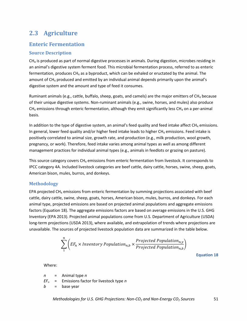
Methodologies for U.S. GHG Projections: Non-CO2 and Non-Energy CO2 Sources 51
2.3 Agriculture
Enteric Fermentation
Source Description
CH4 is produced as part of normal digestive processes in animals. During digestion, microbes residing in
an animal’s digestive system ferment food. This microbial fermentation process, referred to as enteric
fermentation, produces CH4 as a byproduct, which can be exhaled or eructated by the animal. The
amount of CH4 produced and emitted by an individual animal depends primarily upon the animal’s
digestive system and the amount and type of feed it consumes.
Ruminant animals (e.g., cattle, buffalo, sheep, goats, and camels) are the major emitters of CH4 because
of their unique digestive systems. Non-ruminant animals (e.g., swine, horses, and mules) also produce
CH4 emissions through enteric fermentation, although they emit significantly less CH4 on a per-animal
basis.
In addition to the type of digestive system, an animal’s feed quality and feed intake affect CH4 emissions.
In general, lower feed quality and/or higher feed intake leads to higher CH4 emissions. Feed intake is
positively correlated to animal size, growth rate, and production (e.g., milk production, wool growth,
pregnancy, or work). Therefore, feed intake varies among animal types as well as among different
management practices for individual animal types (e.g., animals in feedlots or grazing on pasture).
This source category covers CH4 emissions from enteric fermentation from livestock. It corresponds to
IPCC category 4A. Included livestock categories are beef cattle, dairy cattle, horses, swine, sheep, goats,
American bison, mules, burros, and donkeys.
Methodology
EPA projected CH4 emissions from enteric fermentation by summing projections associated with beef
cattle, dairy cattle, swine, sheep, goats, horses, American bison, mules, burros, and donkeys. For each
animal type, projected emissions are based on projected animal populations and aggregate emissions
factors (Equation 18). The aggregate emissions factors are based on average emissions in the U.S. GHG
Inventory (EPA 2013). Projected animal populations come from U.S. Department of Agriculture (USDA)
long-term projections (USDA 2013), where available, and extrapolation of trends where projections are
unavailable. The sources of projected livestock population data are summarized in the table below.
∑(
)
Equation 18
Where:
n = Animal type n EFn = Emissions factor for livestock type n b = base year

Methodologies for U.S. GHG Projections: Non-CO2 and Non-Energy CO2 Sources 52
Summary of Calculations by Animal Type
Animal Type Population Projection Projected Emissions Factor
Dairy cattle USDA Long-Term Agricultural Projections to 2022 (USDA 2013) and extrapolation
Aggregate emissions factor, extrapolated
Beef cattle USDA Long-Term Agricultural Projections to 2022 (USDA 2013) and extrapolation
Aggregate emissions factor, extrapolated
Swine USDA Long-Term Agricultural Projections to 2022 (USDA 2013) and extrapolation
Fixed
Sheep Historical extrapolation Fixed
Goats Historical extrapolation Fixed
Horses Assumed constant Fixed
American bison Assumed constant Fixed
Mules, burros, and donkeys
Assumed constant Fixed
Activity Data
Projected animal populations come from a combination of USDA projections and extrapolations of
trends.
USDA Long-Term Agricultural Projections provide projections over a 10-year period for various
agricultural information including livestock populations for dairy cattle, beef cattle, and swine. They also
provide production weight for poultry, which is used for projection purposes as a proxy for the number
of poultry. Because the projections in this report extend over a longer period than the USDA projections,
EPA extrapolated livestock populations over the rest of the projection period by applying the same
average percent change between the base year and the end of the USDA projection period to the end of
the USDA projections.
Projected animal populations are not available for sheep, goats, horses, American bison, mules, burros,
and donkeys. In the case of sheep and goats, EPA extrapolated projected future animal populations by
applying the average percent change over the last 10 years of the U.S. inventory to the population in the
base year. The populations of horses, American bison, mules, burros, and donkeys make up a very small
portion of the emissions from this source, and were assumed to remain constant over the projection
period.
The U.S. GHG Inventory uses a more detailed set of beef and dairy populations to estimate livestock
emissions, and therefore the projections presented here do not use identical methodology to estimate
emissions from cattle as the inventory. To estimate CH4 emissions, the inventory relies on EPA’s Cattle
Enteric Fermentation Model (CEFM), which is based on recommendations provided in IPCC guidelines.
The CEFM uses information on population, energy requirements, digestible energy, and CH4 conversion
rates to estimate CH4 emissions. The inventory methodology is more detailed than the methodology for
projections; it uses additional activity data not available for projections, such as counts for younger
replacement dairy and beef cattle of various ages. For example, instead of the “dairy cattle” and “beef
cattle” groupings, the inventory uses 10 different cattle subpopulations based on age:
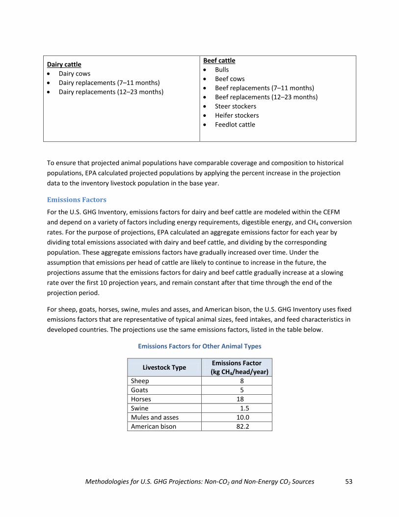
Methodologies for U.S. GHG Projections: Non-CO2 and Non-Energy CO2 Sources 53
Dairy cattle
Dairy cows
Dairy replacements (7–11 months)
Dairy replacements (12–23 months)
Beef cattle
Bulls
Beef cows
Beef replacements (7–11 months)
Beef replacements (12–23 months)
Steer stockers
Heifer stockers
Feedlot cattle
To ensure that projected animal populations have comparable coverage and composition to historical
populations, EPA calculated projected populations by applying the percent increase in the projection
data to the inventory livestock population in the base year.
Emissions Factors
For the U.S. GHG Inventory, emissions factors for dairy and beef cattle are modeled within the CEFM
and depend on a variety of factors including energy requirements, digestible energy, and CH4 conversion
rates. For the purpose of projections, EPA calculated an aggregate emissions factor for each year by
dividing total emissions associated with dairy and beef cattle, and dividing by the corresponding
population. These aggregate emissions factors have gradually increased over time. Under the
assumption that emissions per head of cattle are likely to continue to increase in the future, the
projections assume that the emissions factors for dairy and beef cattle gradually increase at a slowing
rate over the first 10 projection years, and remain constant after that time through the end of the
projection period.
For sheep, goats, horses, swine, mules and asses, and American bison, the U.S. GHG Inventory uses fixed
emissions factors that are representative of typical animal sizes, feed intakes, and feed characteristics in
developed countries. The projections use the same emissions factors, listed in the table below.
Emissions Factors for Other Animal Types
Livestock Type Emissions Factor (kg CH4/head/year)
Sheep 8
Goats 5
Horses 18
Swine 1.5
Mules and asses 10.0
American bison 82.2

Methodologies for U.S. GHG Projections: Non-CO2 and Non-Energy CO2 Sources 54
Manure Management
Source Description
The management of livestock manure can produce anthropogenic CH4 and N2O emissions. When
livestock or poultry manure is stored or treated in systems that promote anaerobic conditions (e.g., as a
liquid/slurry in lagoons, ponds, tanks, or pits), the decomposition of materials in the manure produces
CH4.For non-liquid-based manure systems, moist conditions (which are a function of rainfall and
humidity) can create areas of anaerobic conditions and associated CH4 production. Ambient
temperature, moisture, and manure storage or residency time affect the amount of CH4 produced
because they influence the growth of the bacteria responsible for CH4 formation.
Direct N2O emissions are produced as part of the nitrogen cycle through the nitrification and
denitrification of the organic nitrogen in livestock dung and urine. Specifically, direct N2O emissions
occur when the manure is first handled aerobically and then anaerobically. These emissions are most
likely to occur in dry manure handling systems that have aerobic conditions, but also contain pockets of
anaerobic conditions due to saturation. Indirect N2O emissions are produced when nitrogen is lost from
the system through volatilization or through runoff and leaching. Runoff losses would be expected from
operations that house animals or store manure in a manner that exposes them to weather. (EPA 2013)
This source category covers CH4 and N2O emissions from manure management systems. It corresponds
to IPCC source category 4B. (Emissions associated with pasture, range, and paddock and daily spread
systems are covered in the agricultural soil management source category.) Emissions in this category
include manure from dairy and beef cattle, swine, sheep, goats, poultry, and horses.
Methodology
EPA calculated emissions projections from manure management systems by summing projections of emissions associated with dairy cattle, beef cattle, swine, sheep, goats, poultry, and horses.
∑
Equation 19
Where:
EFaggn,y = Aggregate emissions factor for animal type n in year y
InventoryPopulation = Historical livestock populations from U.S. GHG Inventory ProjectedPopulation = Projected populations from USDA Long-Term Agricultural
Projections y = projected year y b = base year
Emissions Factors
EPA calculated the aggregate emissions factor for past years for each animal type by dividing historical
CH4 and N2O emissions associated with each animal type by the livestock populations. The U.S. GHG

Methodologies for U.S. GHG Projections: Non-CO2 and Non-Energy CO2 Sources 55
Inventory presents these aggregate emissions factors for historical years for CH4 from manure
management (EPA 2013).
The aggregate emissions factor used for projections was calculated differently for different animal types.
In the cases of dairy cattle and swine, changes in animal size and greater use of liquid systems have led
to an increasing trend in emissions from manure management per animal. To capture this trend, EPA
extrapolated projected aggregate emissions factors for these animals based on the average percent
change over the previous 10 years. For beef cattle, sheep, goats, poultry, and horses, no clear trend is
present and the aggregate emissions factor used for projections was the average of the previous five
years, to smooth out year-to-year variations.
Livestock Populations
Projections of dairy cattle, beef cattle, and swine are available as part of the USDA Long-Term
Agricultural Projections, in terms of 1,000 head (USDA 2013). Projections of young chicken production in
million pounds are available as well, which is assumed to be proportional to livestock populations. Long-
term projections are not available for sheep, goats, or horses; EPA extrapolated these from historical
populations or assumed that they were constant.
Summary of Projection Calculations by Animal Type
Animal Type Projection Projected Aggregate Emissions Factor
Dairy cattle USDA population projections, extrapolation Extrapolated
Beef cattle USDA population projections, extrapolation Average of last five years
Swine USDA population projections, extrapolation Extrapolated
Sheep Historical extrapolation Average of last five years
Goats Historical extrapolation Average of last five years
Poultry USDA production projections, extrapolation Average of last five years
Horses Assumed constant Average of last five years

Methodologies for U.S. GHG Projections: Non-CO2 and Non-Energy CO2 Sources 56
Rice Cultivation
Source Description
All rice grown in the United States is grown in flooded fields. When fields are flooded, aerobic
decomposition of organic material gradually depletes most of the oxygen present in the soil, causing
anaerobic soil conditions. Once the environment becomes anaerobic, CH4 is produced through anaerobic
decomposition of soil organic matter by methanogenic bacteria. Factors that influence CH4 emissions
from flooded rice fields include fertilization practices (especially the use of organic fertilizers), soil
temperature, soil type, rice variety, and cultivation practices (e.g., tillage, seeding, and weeding
practices).
This source category covers CH4 emissions from rice cultivation. It corresponds to IPCC source category
4C.
Methodology
Projected emissions from this source are calculated by multiplying (1) an aggregate emissions factor
based on historical emissions per area by (2) base year area harvested from the U.S. GHG Inventory by
(3) projected change in area of harvested rice in the U.S. from base year to the projection year from
USDA long-term projections.
(
)
Equation 20
Where:
EFagg = Aggregate emissions factor
y = Projection year y
b = Base year
Activity Data
The U.S. Department of Agriculture (USDA) Long-Term Agricultural Projections report (USDA 2013)
contains projections of rice area planted, rice area harvested, rice yield per acre, total production, and
various economic information such as imports and exports. The report generally projects U.S. rice
production for Arkansas, California, Louisiana, Mississippi, Missouri, and Texas over a 10-year period.
The U.S. GHG Inventory (EPA 2013) includes Florida and Oklahoma as well; because it adds production
from these two states, there are slight differences in the coverage of historical area used for the
inventory and area projections. To avoid problems cause by these differences, EPA applied the growth
rate in the projection to the base year emissions data.
EPA used rice area harvested for these projections. Projections in this report extend past the 10-year
projection window presented in the USDA long-term projections report, so EPA extrapolated the
projections over the remainder of the projection period by assuming that rice area harvested remained
constant after the end of the period covered by USDA projections. Over the historical period, harvested

Methodologies for U.S. GHG Projections: Non-CO2 and Non-Energy CO2 Sources 57
rice area has fluctuated between about 1.2 and 1.6 million hectares based on shifting market conditions,
making rice more or less valuable relative to other crops. Year-to-year variation has exceeded overall
trends.
Emissions Factor
To calculate an aggregate emissions factor for kilograms of CH4 per hectare of rice harvested, EPA
divided historical emissions by area of harvested rice over the most recent five years of the U.S. GHG
Inventory and averaged the results.
[ ∑ (
)
] ⁄
Equation 21
Where:
EFagg = Aggregate emissions factor
b = Base year
Methodologies for U.S. GHG Projections: Non-CO2 and Non-Energy CO2 Sources 58
Agricultural Soil Management
Source Description
N2O is produced naturally in soils through the microbial processes of nitrification and denitrification. A
number of agricultural activities increase mineral nitrogen availability in soils, thereby increasing the
amount available for nitrification and denitrification, and ultimately the amount of N2O emitted.
Direct increases occur through a variety of management practices that add or lead to greater release of
mineral nitrogen to the soil, including fertilization; application of managed livestock manure and other
organic materials such as sewage sludge; deposition of manure on soils by domesticated animals in
pastures, rangelands, and paddocks; production of nitrogen-fixing crops and forages; retention of crop
residues; and drainage and cultivation of organic cropland soils. Other agricultural soil management
activities, including irrigation, drainage, tillage practices, and fallowing of land, can influence nitrogen
mineralization in soils and thereby affect direct emissions. Indirect emissions of N2O occur through
volatilization and subsequent atmospheric deposition of applied/mineralized nitrogen, as well as surface
runoff and leaching of applied/mineralized nitrogen into groundwater and surface water.
This source category includes direct and indirect N2O emissions from croplands and grasslands. This
source category corresponds to IPCC source category 4D.
Methodology
To project N2O emissions from agricultural soil management, EPA allocated base year emissions from
this source to subcategories associated with various activity drivers, and then using changes in the
projections of those activity drivers from the base year to scale the base year inventory emissions. The
activity drivers identified are (1) nitrogen from synthetic fertilizer use, (2) residues from crop production,
and (3) livestock manure (both managed and unmanaged pasture, range, and paddock).
(
)
Equation 22
Where:
Emissionss,y = N2O emissions for source s in year y
Activitys,y = Activity driver associated with source s in year y (kg N)
The U.S. inventory divides emissions using the following categories:
1. Direct N2O emissions
o Cropland soils
Mineral soils
Synthetic fertilizer
Organic amendment

Methodologies for U.S. GHG Projections: Non-CO2 and Non-Energy CO2 Sources 59
Residue N
Mineralization and asymbiotic fixation
Organic soils
o Grassland soils
Synthetic fertilizer
Pasture, range and paddock (PRP) manure
Managed manure
Sewage sludge
Residue N
Mineralization and asymbiotic fixation
2. Indirect N2O emissions
o Land type
Cropland, grassland, forest land, settlements
o Emissions type
Volatilization and atmospheric deposition
Leaching/runoff
For the purpose of projections, emissions subcategories are aggregated as indicated in the table below
for association with various activity data drivers:
Inventory Subcategory Activity Data Driver
for Projections Projection Source
Direct emissions from synthetic N fertilizer use on mineral cropland soils and grassland soils
Fertilizer use Extrapolation of historical usage
Direct emissions from organic N amendments on mineral cropland soils and direct emissions from PRP manure N and managed manure N on grasslands
Livestock production
USDA projections of livestock production and populations (USDA 2013)
Direct emissions from crop residue N on mineral cropland soils and grasslands
Crop production USDA projections of crop production (USDA 2013) multiplied by default IPCC 2006 factors for dry matter and N content (IPCC 2006)
All other direct emissions (mineralization and asymbiotic fixation on mineral soils, organic soils, and sewage sludge; mineralization and asymbiotic fixation on grasslands)
None Held constant
Indirect emissions total Direct emissions (less mineralization and asymbiotic fixation)
Proportional to sum of direct emissions calculations for synthetic fertilizer, organic amendments, crop residue N, and other except mineralization and asymbiotic fixation

Methodologies for U.S. GHG Projections: Non-CO2 and Non-Energy CO2 Sources 60
Synthetic Fertilizer Use
EPA calculated projected synthetic fertilizer use by calculating the average percent change in historic
synthetic fertilizer use over the previous 10 years and applying that percentage change over the
projection period. The U.S. GHG Inventory (EPA 2013) includes data used for past emissions inventories
on synthetic fertilizer nitrogen added to major and non-major crops, which EPA summed for this
calculation.
Synthetic fertilizer use projections are not available from USDA as part of the Long-Term Agricultural
Projections, although crop production and other projections are available. Synthetic fertilizer use
projections are provided by the Food and Agricultural Policy Research Institute at Iowa State University
(FAPRI 2011), but were not used directly for these projections. These projections are used as a
comparison to the historical extrapolation. Another alternative source for projecting nitrogen fertilizer
usage is examining historical trends in crop production and fertilizer use and extrapolating those
individual trend relationships.
Nitrogen from Crop Residues
Projected nitrogen from crop residues is calculated using (1) projected production amounts and
harvested acreage of various crop types from USDA long-term projections and (2) default factors from
IPCC 2006 guidelines for harvested annual dry matter yield, ratios of above- and below-ground residue
to harvested yield, and nitrogen contents of above- and below-ground residue (IPCC 2006). Standard
bushel weight factors convert bushel production to weight measures. The Tier 1 equation from the IPCC
guidelines is used to calculate nitrogen from crop residues.
Crop production projections are available from USDA long-term projections for corn, sorghum, barley,
oats, wheat, soybeans, rice, cotton, and sugar. The inventory calculates emissions associated with both
major and non-major crops. Major crops make up more than 90 percent of U.S. cropland, so the
production trend for major crops is taken to represent the overall trend for the purpose of N2O
emissions projections associated with crop residues.
∑ [ ( )]
adapted from IPCC (2006), Equation 11.7a
Equation 23
Where:
c = Crop type Hc = Harvested annual dry matter yield for crop c Rag,c = Ratio of above-ground dry matter residues to harvested yield for crop c Nag,c = N content of above-ground residues for crop c Rbg,c = Ratio of below-ground dry matter residues to harvested yield for crop c Nbg,c = N content of below-ground residues for crop c

Methodologies for U.S. GHG Projections: Non-CO2 and Non-Energy CO2 Sources 61
The IPCC 2006 guidelines describe Tier 1 equations and default factors to calculate average crop residue
from different crop types using dry matter fractions, above- and below-ground ratios of residues to dry
matter fraction of harvested product, and nitrogen content of above- and below-ground residues. In
addition to major crop types, default factors are provided for individual crop types. These default factors
are found in table 11.2 of the IPCC 2006 guidelines.
Nitrogen from Livestock Manure
Projected nitrogen from livestock manure applied to croplands and grasslands (through either managed
or unmanaged pathways) is calculated using (1) USDA projections of various livestock populations and
(2) default factors for nitrogen excretion and typical animal mass from the IPCC (2006) guidelines.
Projected livestock populations are used consistent with the assumptions detailed in the manure
management source category methodology. (Dairy, beef, swine, and poultry populations are from USDA
Long Term projections; other animal type populations are extrapolated, and horse populations are
assumed to be constant.) Default excretion rates for the various animal types are multiplied by the
projected animal populations to estimate manure from livestock. The proportion of manure generation
added to each crop type and cropland versus grassland is assumed to be constant.

Methodologies for U.S. GHG Projections: Non-CO2 and Non-Energy CO2 Sources 62
2.4 Land Use, Land-Use Change, and Forestry
CH4 and N2O Emissions from Forest Fires
Source Description
GHG fluxes occur due to changes within and conversions between certain land-use types, such as forest
land, cropland, grassland, settlements, and wetlands.
The GHG flux from Forest Land Remaining Forest Land is reported under the 2006 IPCC Guidelines (IPCC
2006) using estimates of changes in forest carbon stocks, non-CO2 emissions from forest fires (CH4 and
N2O), and the application of synthetic fertilizers to forest soils. This section focuses on the non-CO2 GHG
emissions associated with forest fires (both wildfires and prescribed fires). Changes in forest C stock are
beyond the scope of this report.
Methodology
EPA projected CH4 and N2O emissions from forest fires by multiplying projected forest hectares burned
by historical average carbon density factors, default IPCC combustion rates, and ratios of CH4 and N2O
emissions to CO2 emissions. Projections of area burned are drawn from an average of several model
estimates from research in press (Mills et al. n.d.).
Projections of Forest Fires
Wildfire projections for the lower 48 states were estimated using modeling results from Mills et al.
(n.d.). This analysis applied the MC-1 dynamic global vegetation model with climate projection data
from two general circulation models (GCMs) and three emissions scenarios (“business as usual” and two
exemplary global GHG mitigation policies). MC-1 provides gridded results at varying spatial and
temporal scales that can inform plant and leaf types, nutrient movement, and vegetation disturbance by
wildfire. MC-1’s fire model simulates wildfire’s occurrence, its behavior, and some of its ecosystem
effects.19 The fire model calculates the fraction of a half-kilometer-by-half-kilometer cell’s area that is
burned over different lengths of time (e.g., annually, multi-year periods) as a function of the simulated
rate of fire spread and the amount of time since the last fire event. The corresponding area burned in a
cell is then calculated by multiplying the fraction burned by the cell area. MC1 output was adjusted to
exclude the proportion of any cell assumed to be in developed or agricultural land use types.20
19
While the MC1 fire model is meant to simulate natural fire dynamics, human activity (specifically fire suppression policies) clearly has had a dramatic impact on recent fire frequency and intensity. The fire model accounts for this by incorporating a fire suppression adjustment, which assumes that 95 percent of fires that would have otherwise naturally occurred have been suppressed. For the remaining unsuppressed fires, the methodology assumes that those above a defined fireline intensity burn 95 percent of affected areas. While this rule does not capture the subtleties of 20
th century fire suppression, it can reproduce patterns of historical fires in the United
States reasonably well. It is also important to note that proactive fire suppression (e.g., prescribed fires) and other management activities were not modeled in the analysis (Mills et al. n.d.).
20 Developed lands were projected using the Integrated Climate and Land Use Scenarios (ICLUS; Bierwagen et al.
2010) model. Using the U.S. population projections described in Paltsev et al. (n.d.), the ICLUS model generated county-level population projections at five-year intervals between 2000 and 2100.
The spatial allocation submodel
Methodologies for U.S. GHG Projections: Non-CO2 and Non-Energy CO2 Sources 63
Mills et al. estimated the acreage burned in the lower 48 states from wildfires, aggregated both by
region and national total, using two GCMs under a “business as usual” or reference scenario. These
GCMs were selected to reasonably bound the future variation in mean temperature and precipitation in
the United States. The two GCMs—CCSM-30 and MIROC-MED—comparatively project a generally
cool/wet (although still warmer than the baseline) and hot/dry future climate, respectively, for the
lower 48.
The acreage burned through in the lower 48 states from prescribed fires and from wildfires in Alaska
was not available. Therefore, the average acreage burned for the five most recent inventory years,
specifically regarding prescribed fires in the lower 48 and all wildfires in Alaska, was determined and
assumed to remain constant through 2035.
Carbon Emitted
Estimates for carbon emitted21 include emissions from wildfires in both Alaska and the lower 48 states,
as well as emissions from prescribed fires in the lower 48 states only (based on expert judgment that
prescribed fires only occur in the lower 48 states). EPA applied the IPCC (2006) default combustion
factor of 0.45 for “all ‘other’ temperate forests” in estimating C emitted from both wildfires and
prescribed fires. Mills et al. provide total area burned (not just forest) and so the average ratio of forest
area to total area burned over the previous five years was applied, resulting in projections of forest area
burned.
As stated in the U.S. GHG Inventory (EPA 2013), the emissions factors for the three categories of forest
fires are:
Wildfires in the lower 48 states: 31.7 to 34.4 megagrams carbon per hectare
Wildfires in Alaska: 63.3 to 64.4 megagrams carbon per hectare
Prescribed fires in lower 48 states: 11.4 to 11.7 megagrams carbon per hectare
For the projections, the average of each emissions factor was used. It was assumed that these emissions
factors remain constant through the end of the projection period.
within ICLUS then applied the county projections into developed and undeveloped lands in the future at a resolution of 1 square kilometer. Pixels were designated as “developed” if they contained more than one housing unit per 40 acres, or if the pixel was pre-established in ICLUS as being commercial/industrial land. Pixels with less than one housing unit per 40 acres were classified as “undeveloped.” Agricultural areas were derived from the 2001 National Land Cover Database (USGS 2003), and assumed static for the entirety of the study period—thus using current agricultural land use to screen out areas that are currently intensively managed. The agricultural and
developed lands layer was combined with the coarser-resolution data from MC1 (0.5 × 0.5/ ~1,600 km2
resolution) to determine the proportion of land types within the MC1 cell. Mills et al. (n.d.): (1) recognized that agricultural land use patterns will likely change significantly in the future, but found that credible and spatially explicit estimates were limited; (2) recognized that while agricultural areas contribute significantly to terrestrial C storage, the focus of this paper is on carbon and wildfire dynamics in natural areas; and (3) recognized that carbon dynamics in agricultural areas are more appropriately analyzed using other models developed specifically for these systems.
21 Carbon emitted = emissions factor (in megagrams carbon per hectare) multiplied by hectares burned.

Methodologies for U.S. GHG Projections: Non-CO2 and Non-Energy CO2 Sources 64
Conversion Factors
To estimate CO2 emissions, EPA multiplied total carbon emitted by the C to CO2 conversion factor of
44/12 and by 92.8 percent, which is the estimated proportion of carbon emitted as CO2. Projections of
carbon emitted from forest fires are drawn from an average of several model estimates from research in
press (Mills et al. n.d.).
(
)
Equation 24
Where:
ECH4,y = Total annual CH4 emissions from forest fires for year y
EC,y = Total annual C emissions from forest fires for year y
92.8% = Estimated proportion of C emitted as CO2
44/12 = Molecular weight ratio of CO2 to C
ERCH4,y = Emissions ratio of CH4 to CO2 for year y
(
)
Equation 25
Where:
EN2O,y = Total annual N2O emissions from forest fires for year y
EC,y = Total annual C emissions from forest fires for year y
92.8% = Estimated proportion of C emitted as CO2
44/12 = Molecular weight ration of CO2 to C
ERN2O,y = Emissions ratio of N2O to CO2 for year y
Default emissions ratios between CH4, N2O, and CO2 are calculated based on emissions factors for
burning of forests. Default emissions rates for forests other than tropical forests are 1,569 grams of CO2,
4.7 grams of CH4, and 0.26 grams of N2O per kilogram of dry matter.22
22
Table 2.5 within Section 2.4 of Volume 4, Chapter 2, of the 2006 IPCC inventory guidelines.

Methodologies for U.S. GHG Projections: Non-CO2 and Non-Energy CO2 Sources 65
2.5 Waste
Landfills
Source Description
Municipal solid waste (MSW) placed in a landfill is initially decomposed by aerobic bacteria. After the
oxygen has been depleted, the remaining waste is available for consumption by anaerobic bacteria,
which break down organic matter into substances such as cellulose, amino acids, and sugars. These
substances are further broken down through fermentation into gases and short-chain organic
compounds that form the substrates for the growth of methanogenic bacteria. These CH4-producing
anaerobic bacteria convert the fermentation products into stabilized organic materials and biogas
consisting of approximately 50 percent biogenic CO2 and 50 percent CH4, by volume, with less than 1
percent non-methane organic compounds and trace amounts of inorganic compounds. Significant CH4
production typically begins one or two years after waste disposal in a landfill and continues for 10 to 60
years or longer as the degradable waste decomposes over time (EPA 2013).
CH4 emissions from landfills are a function of several factors, including (1) the total amount of waste in
MSW landfills, which is related to total waste landfilled annually; (2) the characteristics of landfills
receiving waste (i.e., composition of waste-in-place, size, climate); (3) the amount of CH4 that is
recovered and either flared or used for energy purposes; and (4) the amount of CH4 oxidized in landfills
instead of being released into the atmosphere.
This source category covers fugitive CH4 emissions from landfills. It corresponds to IPCC source category
6A1.
Methodology
EPA calculated emissions projections for this source by (1) projecting potential emissions from MSW
landfills, (2) adding potential emissions from industrial landfills, and then (3) subtracting CH4 recovered
from gas-to-energy projects or flared CH4 and (4) subtracting oxidized CH4.
( )
Equation 26
Where:
Etl,y = Projected total annual CH4 emissions from landfills for year y
PEml,y = Potential emissions from MSW landfills for year y
PEil,y = Potential emissions from industrial landfills for year y
Er,y = Annual CH4 emissions recovered for year y
Ox = Percent oxidation (%)
MSW Landfills
EPA projected potential CH4 emissions from MSW landfills using the integrated form of the first order
decay (FOD) model, which uses the procedures and spreadsheets from IPCC (2006) to estimate CH4

Methodologies for U.S. GHG Projections: Non-CO2 and Non-Energy CO2 Sources 66
emissions from solid waste disposal. EPA used a form of the FOD model that incorporates a time delay
of six months after waste disposal before the generation of CH4 begins. FOD models assume that landfill
CH4 generation is at its peak shortly after initial placement. The input parameters required for the FOD
model equations are:
The mass of waste disposed of each year. The historical amount of “MSW landfilled” and “waste in
place” were taken from the U.S. GHG Inventory (EPA 2013). To project annual landfill waste
generation and disposal data for the United States through the end of the projection period, EPA
compared historical MSW disposal rates to landfills and the U.S. population, resulting in per capita
rates of landfill MSW disposal. EPA took historical MSW disposal rates for the United States from the
U.S. GHG Inventory and historical U.S. population data from the U.S. Census Bureau for the
corresponding years (U.S. Census 2011). Based on the historical trend, EPA assumed the per capita
rate of landfill MSW disposal for the projections to be the average of the last four years of the most
recent U.S. GHG Inventory.
To project the annual MSW disposed of in landfills each year, EPA multiplied the per capita rate of
landfill MSW disposal by the projected U.S. population data from the U.S. Census Bureau (U.S.
Census 2012). Per capita waste disposal was assumed to remain constant over the projection period.
The degradable organic carbon (DOC). The DOC (fraction, gigagrams carbon per gigagram of waste)
was assumed to remain constant at the value presented in the most recent U.S. GHG Inventory
through the end of the projection period.
The CH4 generation potential (L0) and rate constant (k). The CH4 generation potential (L0 in cubic
meters of CH4 per megagram of waste) and rate constant k (per year) are assumed to remain
constant at the values presented in the most recent U.S. GHG Inventory.
Industrial Landfills
It has been determined that over 99 percent of the organic waste placed in industrial landfills originated
from two industries: food processing (meat, vegetables, fruits) and pulp and paper (EPA 1993).
Therefore, the CH4 emissions from industrial landfills were projected based on the estimated change in
production for both sectors. Specifically, the EIA provides “value of shipments” projections for the food
and paper industries in the Annual Energy Outlook (AEO) reports (EIA 2013). The annual percent
increase or decrease in “value of shipments” was assumed to be approximately equivalent to the annual
percent change in production for the two industries.23 The most recent inventory year served as the
baseline for the CH4 emissions projections.
23 As discussed in the 2013 U.S. GHG Inventory, not all of the items produced from the food processing and pulp and paper industry are deposited in a landfill. Research into waste generation and disposal in landfills for the pulp and paper industry indicated that the quantity of waste landfilled was about 0.050 megagrams per megagram of product compared to 0.046 megagrams per megagram product for the food processing industry (Weitz and Bahner 2006). However, since the historical CH4 emissions from industrial landfills contained in the 2013 U.S. GHG Inventory already account for this, EPA did not apply the ratio directly to future projections. EPA also assumed a constant emissions factor for projection purposes.

Methodologies for U.S. GHG Projections: Non-CO2 and Non-Energy CO2 Sources 67
(
)
Equation 27
Where:
PEil,y = Potential emissions from industrial landfills for year y
PEil,b = Potential emissions from industrial landfills for base year b
VSfp,y = Value of shipments for food and paper industries for year y
VSfp,b = Value of shipments for food and paper industries for base year b
Note that the CH4 emissions from industrial landfills for the most recent year addressed in the U.S. GHG
Inventory serves as the baseline year for the emissions projections.
Recovered CH4 from Gas-to-Energy and Flaring
The U.S. GHG Inventory accounts for CH4 emissions avoided (i.e., recovered) due to landfill-gas-to-energy
(LFGTE) projects and flaring. To project recovered CH4 emissions, EPA extrapolated the historical percent
of CH4 generation recovered (as stated in the most recent U.S. GHG Inventory) through the end of the
projection period. EPA then subtracted these recovered CH4 emissions from the total annual CH4
emissions projected from MSW landfills. The projected recovery and flaring ratio will be cross-checked
against more detailed landfill-level modeling to ensure that it properly reflects industry practices and
regulatory requirements.
Oxidized CH4 from Landfills Prior to Release to Atmosphere
A portion of the CH4 escaping from a landfill oxidizes to CO2 in the top layer of the soil. The amount of
oxidation depends upon the characteristics of the soil and the environment. Similar to the U.S. GHG
Inventory, it was assumed that 10 percent of the CH4 generated (minus the amount of gas recovered for
flaring or LFGTE projects) was oxidized in the soil. The factor of 10 percent is consistent with the value
recommended in the IPCC (2006) revised guidelines for managed and covered landfills, and was
therefore applied to the estimates of CH4 generation minus recovery for both MSW and industrial
landfills.

Methodologies for U.S. GHG Projections: Non-CO2 and Non-Energy CO2 Sources 68
Domestic Wastewater Treatment
Source Description
The treatment of domestic wastewater can result in CH4 and N2O emissions. Wastewater from domestic
sources24 is treated to remove soluble organic matter, suspended solids, pathogenic organisms, and
chemical contaminants. Wastewater treatment is conducted either on site, most commonly through the
use of septic systems or package plants, or off site at centralized treatment systems.
CH4 is produced when organic matter is degraded under anaerobic conditions. The principal factor in
determining the CH4 generation potential of wastewater is the amount of degradable organic material in
the wastewater.
N2O can be generated by the further treatment of domestic wastewater during nitrification and
denitrification of the nitrogen present, usually in the form of urea, ammonia, and proteins. The principal
factor in determining the N2O generation potential of wastewater is the amount of nitrogen in the
wastewater.
This source category covers CH4 and N2O from domestic wastewater treatment systems. This
corresponds to IPCC source category 6B2 (or IPCC 2006 category 4D1). For the purpose of projections,
CH4 emissions from industrial wastewater treatment are treated as a separate source (IPCC category
6B1 or 4D2 in 2006 categories). No source-specific methodology was developed for industrial
wastewater treatment, so the default extrapolation approach was used for that source.
Methodology
Projected emissions from this source category were calculated by summing emissions from various
waste treatment systems: onsite/septic systems, centrally treated aerobic systems, centrally treated
anaerobic systems, and emissions from anaerobic digesters. The total amount of waste is based on
projections of population growth, while the portion of waste attributable to various streams is based on
extrapolating historical trends. The methodology contained in the U.S. GHG Inventory (EPA 2013) was
used as the basis for projecting non-CO2 GHG emissions (CH4 and N2O) from domestic wastewater
treatment.
Domestic Wastewater CH4 Emissions
CH4 emissions can arise from lack of containment or gas collection on septic systems, aerobic systems
that are not well managed or that are designed to have periods of anaerobic activity (e.g., constructed
wetlands), anaerobic systems (anaerobic lagoons and facultative lagoons), and anaerobic digesters
when the captured biogas is not completely combusted. In order to account for these potential CH4
emissions sources, these projections use five pathways for domestic wastewater treatment:
On site (septic systems)
24 As with the U.S. GHG Inventory, EPA assumed that domestic wastewater includes wastewater from household use, as well as any commercial and non-hazardous industrial wastewater that is collected by centralized treatment systems.

Methodologies for U.S. GHG Projections: Non-CO2 and Non-Energy CO2 Sources 69
Centrally treated aerobic systems (with and without primary sedimentation)
Centrally treated anaerobic systems (with and without primary sedimentation)
While anaerobic digestion is not considered a “pathway,” it is an optional treatment process for sludge
after it has gone through a centrally treated aerobic or anaerobic system. Therefore, the CH4 produced
by anaerobic digesters is included in the U.S. GHG Inventory as well as in the emissions projections.
Onsite (Septic Systems)
CH4 emissions from septic systems were estimated in the U.S. GHG Inventory by multiplying the United
States population by the percent of domestic wastewater treated in septic systems and a septic system-
specific emissions factor (10.7 grams CH4/capita/day). To estimate future CH4 emissions from septic
systems, EPA used (1) projected population from the U.S. Census Bureau (U.S. Census 2012) and (2) the
percent of domestic wastewater treated in septic systems/onsite (historical data extrapolation; EPA
2013).
Equation 28
Where:
Ess,y = Total annual CH4 emissions from onsite septic systems for year y (Gg)
POPy = U.S. population for year y (people)
WWos,y = Fraction of domestic wastewater treated onsite (i.e., in septic systems) for year y
(%)
EFss = Septic system-specific emissions factor (grams CH4/person/day)
365.25 = Days per year
109 = Conversion factor (g to Gg)
Centrally Treated Aerobic Systems and Anaerobic Systems
The total BOD content of influent domestic wastewater is assumed to be constant throughout the
central treatment pathways. Therefore, CH4 emissions are proportional to the allocation of wastewater
to each central treatment pathway. For the centrally treated systems, CH4 emissions were estimated in
the U.S. GHG Inventory using the generalized equation below. The emissions factors/correction factors
(EF) and the percent of BOD removed for each pathway distinguish the CH4 generation potential
between aerobic, anaerobic, and with/without primary treatment.
∑[ ]
Equation 29
Methodologies for U.S. GHG Projections: Non-CO2 and Non-Energy CO2 Sources 70
Where:
Ect,y = Total annual CH4 emissions from centrally treated systems (aerobic and anaerobic) for year y
BODtot,y = Total produced BOD for year y WWj,y = Fraction of wastewater treated through pathway j for year y %Rj,y = Fraction of BOD removed through pathway j for year y EFj,y = CH4 emissions factor for pathway j for year y J = Wastewater treatment pathways: onsite, centrally treated aerobic and anaerobic,
with or without primary sedimentation
Equation 30
Where:
BODtot,y = Total produced BOD for year y (kg)
POPy = U.S. population for year y (people)
BODpc,y = Per capita BOD production for year y (kg BOD/person/day)
365.25 = Days per year
To estimate future CH4 emissions from centrally treated systems, EPA projected the following variables:
The U.S. population for each year (U.S. Census 2012).
The percent of domestic wastewater collected (historical data extrapolation; EPA 2013).
The percent of centralized wastewater treatment using aerobic versus anaerobic systems (historical
data extrapolation; EPA 2013).
Other factors, such as emissions factors, were held constant from the most recent inventory year.
Anaerobic Digesters
CH4 emissions from anaerobic digesters were estimated in the U.S. GHG Inventory by multiplying the
wastewater influent flow to centrally treated systems that have anaerobic digesters, the amount of
biogas generated by wastewater sludge treated in anaerobic digesters, the proportion of CH4 in digester
biogas, and the destruction efficiency associated with burning the biogas in an energy/thermal device.
To estimate future CH4 emissions from anaerobic digesters, the following variable was projected:
The influent wastewater flow to centrally treated systems with anaerobic digesters (historical data
extrapolation; EPA 2013).
(
) ⁄
Equation 31

Methodologies for U.S. GHG Projections: Non-CO2 and Non-Energy CO2 Sources 71
Where:
Ead,y = Total annual CH4 emissions from anaerobic digesters for year y (Gg)
WWad,y = Wastewater influent flow to POTWs with anaerobic digesters (gallons)
DGpc,y = Per capita digester gas produced per day (ft3/person/day)
WWpc,y = Per capita wastewater flow to POTW per day (gallons/person/day)
0.0283 = Conversion factor (ft3 to m3)
BG = Proportion of CH4 in biogas
365.25 = Days per year
ρCH4 = Density of CH4 (662 g/m3)
DE = CH4 destruction efficiency from flaring or burning in engine
1/109 = Conversion factor (g to Gg)
Domestic Wastewater N2O Emissions
N2O emissions from domestic wastewater were estimated in the U.S. GHG Inventory using the 2006 IPCC
Guidelines (IPCC 2006). The IPCC methodology includes calculations for the N2O emissions associated
with wastewater effluent discharged to aquatic environments and total N2O emissions from centralized
wastewater treatment plants (with and without nitrification/denitrification). Due to high uncertainty of
measures of N2O from septic systems, estimates of N2O emissions from septic systems were not
included in the U.S. GHG Inventory or these projections (EPA 2013).
Effluent Discharge
N2O emissions from effluent discharge are based on annual, per capita protein consumption (kilograms
of protein per person per year). For the U.S. GHG Inventory, the amount of protein available to be
consumed was estimated based on per capita annual food availability data and the protein content of
that particular food, and then adjusted using a factor to account for the fraction of protein actually
consumed. Any nitrogen removed with sludge, and therefore not discharged to aquatic environments,
was not included.
In the U.S. GHG Inventory, N2O effluent emissions were calculated by multiplying the U.S. population
using central treatment systems (minus the percent of the U.S. population served by biological
denitrification systems) by the annual per capita protein consumption with correction factors, and
subtracting the amount of nitrogen removed with sludge. To estimate future N2O emissions (2011 to
2035) from effluent discharge, EPA projected the following variables:
The U.S. population for each year (U.S. Census 2012).
The U.S. population that is served by biological denitrification (historical data extrapolation; EPA
2013).
The percent of the U.S. population using central treatment systems/plants (historical data
extrapolation; EPA 2013).
Methodologies for U.S. GHG Projections: Non-CO2 and Non-Energy CO2 Sources 72
Annual per capita protein consumption (average of most recent five years).
The amount of nitrogen removed with sludge (assumed to remain constant).
{[((( ) ( )) ) ]
⁄ } ⁄
Equation 32
Where:
N2Oeff,y = Projected total annual N2O emissions from wastewater effluent discharged to
aquatic environments for year y (Gg)
POPy = U.S. population for year y (people)
Ftp,y = Fraction of population using wastewater treatment plant for year y (%)
0.9 = Fraction of nitrogen removed by denitrification systems
POPdn,y = Population that is served by biological denitrification for year y (%)
Proy = Annual per capita protein consumption for year y (kg/person/year)
NPro = Fraction of nitrogen in protein (kg N/kg protein)
Fnc = Factor for non-consumed protein added to wastewater
Fic = Factor for industrial and commercial co-discharged protein into sewer system
Ns,y = Nitrogen removed with sludge for year y (kg N/year)
EFeff = Emissions factor from effluent (kg N2O-N/kg sewage-N produced)
44/28 = Molecular weight ratio of N2O to N2
1/106 = Conversion factor (kg to Gg)
Central Treatment Systems/Plants
N2O emissions from centralized treatment systems include plants that have nitrification/denitrification
as part of their treatment process, as well as plants that do not. EPA calculated N2O emissions from
plants that have nitrification/denitrification by multiplying the U.S. population served by biological
denitrification, an IPCC emissions factor, and a factor for industrial and commercial protein co-
discharged into the sewer system. For N2O emissions from plants that do not have
nitrification/denitrification, EPA multiplied the remainder of the U.S. population that uses central
treatment systems by an IPCC emissions factor and the same factor for industrial and commercial
protein co-discharged into the sewer system. To estimate future N2O emissions (2011 to 2035) from
central treatment systems, EPA projected the following variables:
The U.S. population for each year (U.S. Census 2012).
Fraction of the U.S. population using central treatment plants (historical data extrapolation; EPA
2013).
U.S. population that is served by biological denitrification (historical data extrapolation; EPA 2013).

Methodologies for U.S. GHG Projections: Non-CO2 and Non-Energy CO2 Sources 73
{ ⁄ } {[( ) ] }
⁄
Equation 33
Where:
N2Opl,y = N2O emissions from centralized wastewater treatment plants for year y (Gg)
N2Ond,y = N2O emissions from centralized wastewater treatment plants with
nitrification/denitrification for year y (Gg)
N2Owond,y = N2O emissions from centralized wastewater treatment plants without
nitrification/denitrification for year y (Gg)
POPdn,y = Population that is served by biological denitrification for year y (%)
EFid = Emissions factor for plant with intentional denitrification (g N2O/person/yr)
Fic = Factor for industrial and commercial co-discharged protein into sewer system
POPy = U.S. population for year y (people)
Ftp,y = Fraction of population using wastewater treatment plant for year y (%)
EFnid = Emissions factor for plant with no intentional denitrification (g N2O/person/yr)
1/109 = Conversion factor (g to Gg)
The equations and factors presented in this section are based on those presented within the wastewater
treatment section of the U.S. GHG Inventory, and more information can be found there.

Methodologies for U.S. GHG Projections: Non-CO2 and Non-Energy CO2 Sources 74
3.0 References
Bierwagen, B.G., D.M. Theobald, C.R. Pyke, A. Choate, P. Groth, J.V. Thomas, and P. Morefield (2010)
“National Housing and Impervious Surface Scenarios for Integrated Climate Impact Assessments.”
Proceedings of the National Academy of Sciences 107(49): 20887–20892.
EIA (2012) Annual Coal Report 2011. Available online at <http://www.eia.gov/coal/annual/>.
EIA (2013) Annual Energy Outlook 2013. Available online at <http://www.eia.gov/forecasts/aeo/>.
EPA (1993) Anthropogenic Methane Emissions in the United States, Estimates for 1990: Report to
Congress. EPA-430-R-93-003.
EPA (2010) MOVES2010 Highway Vehicle Population and Activity Data. EPA-420-R-10-026. Available
online at <http://www.epa.gov/otaq/models/moves/420r10026.pdf>.
EPA (2011) Oil and Natural Gas Sector: Standards of Performance for Crude Oil and Natural Gas
Production, Transmission, and Distribution: Background Technical Support Document for the Proposed
Standards. Available online at <http://epa.gov/airquality/oilandgas/pdfs/20110728tsd.pdf>.
EPA (2012a) Oil and Natural Gas Sector: New Source Performance Standards and National Emission
Standards for Hazardous Air Pollutants Reviews. 40 CFR Parts 60 and 63 [EPA-HQ-OAR-2010-0505; FRL-
9665-1], RIN 2060-AP76. Available online at <http://www.gpo.gov/fdsys/pkg/FR-2012-08-16/pdf/2012-
16806.pdf>.
EPA (2012b) Oil and Natural Gas Sector: Standards of Performance for Crude Oil and Natural Gas
Production, Transmission, and Distribution: Background Supplemental Technical Support Document for
the Final New Source Performance Standards.z Available online at
<http://epa.gov/airquality/oilandgas/pdfs/20120418tsd.pdf>.
EPA (2012c) Natural Gas STAR Reductions 1990-2011. Natural Gas STAR Program.
EPA (2012d) Updates to the Greenhouse Gas and Energy Consumption Rates in MOVES2010a. EPA-420-
R-12-025. Available online at <http://www.epa.gov/otaq/models/moves/documents/420r12025.pdf>.
EPA (2013) Inventory of U.S. Greenhouse Gas Emissions and Sinks: 1990–2011. EPA-430-R-13-001.
Available online at <http://www.epa.gov/climatechange/ghgemissions/usinventoryreport.html>.
FAPRI (2011) FAPRI-ISU 2012 World Agricultural Outlook. Available online at
<http://www.fapri.iastate.edu/outlook/2012/>.
IPCC (2006) 2006 IPCC Guidelines for National Greenhouse Gas Inventories. Available online at
<http://www.ipcc-nggip.iges.or.jp/public/2006gl/>.
Methodologies for U.S. GHG Projections: Non-CO2 and Non-Energy CO2 Sources 75
Marks, J., and C. Bayliss (2010) “Aluminum—Meeting the Challenge of Climate Change.” Journal of the
Minerals, Metals & Materials Society 62(8): 33–36. Available online at
<http://www.tms.org/pubs/journals/jom/1008/marks-1008.html>.
Mills, D., R. Jones, K. Carney, A. St. Juliana, R. Ready, A. Crimmins, J. Martinich, K. Shouse, B. DeAngelo,
and E. Monier (n.d.) “Climate Change Impacts on Terrestrial Ecosystems and Forests in the United
States.” Climatic Change. In review.
Montzka, S.A., L. Kujipers, M.O. Battle, M. Aydin, K.R. Verhulst, E.S. Saltzman, and D.W. Fahey (2010) “Recent Increases in Global HFC-23 Emissions.” Geophysical Research Letters 37(2), L02808, doi:10.1029/2009GL041195.
Paltsev, S., E. Monier, J. Scott, A. Sokolov, J. Reilly, X. Gao, and A. Schlosser (n.d.) “Integrated Economic
and Climate Projections for Impact Assessment.” Climatic Change. In review.
U.S. Census (2011) Population Estimates. Available online at <http://www.census.gov/popest/data/historical/index.html>.
U.S. Census (2012) 2012 National Population Projections. Available online at <http://www.census.gov/population/projections/data/national/>.
USDA (2013) USDA Agricultural Projections to 2022. Long-Term Projections Report OCE-2013-1.
Available online at <http://www.ers.usda.gov/publications/oce-usda-agricultural-
projections/oce131.aspx#.UXAmW7WG18E>.
USGS (2003) National Land Cover Database 2001. Available online at
<http://landcover.usgs.gov/uslandcover.php>.