1

Methodological Foundation of a Numerical Taxonomy of Urban

Form

Martin FLEISCHMANN

Department of Geography and Planning, University of Liverpool, Roxby Building, Liverpool,

L69 7ZT, United Kingdom. m.fleischmann@liverpool.ac.uk; +44(0)7482 082 1247;

Corresponding author

Department of Architecture, University of Strathclyde

Alessandra FELICIOTTI

Department of Architecture, University of Strathclyde, a.feliciotti@strath.ac.uk

Ombretta ROMICE

Department of Architecture, University of Strathclyde, ombretta.r.romice@strath.ac.uk

Sergio PORTA

Department of Architecture, University of Strathclyde, sergio.porta@strath.ac.uk

2

Methodological Foundation of a Numerical Taxonomy of Urban

Form

Abstract

Cities are complex products of human culture, characterised by a startling diversity of visible

traits. Their form is constantly evolving, reflecting changing human needs and local

contingencies, manifested in space by many urban patterns.

Urban Morphology laid the foundation for understanding many such patterns, largely relying

on qualitative research methods to extract distinct spatial identities of urban areas. However,

the manual, labour-intensive and subjective nature of such approaches represents an

impediment to the development of a scalable, replicable and data-driven urban form

characterisation. Recently, advances in Geographic Data Science and the availability of

digital mapping products, open the opportunity to overcome such limitations. And yet, our

current capacity to systematically capture the heterogeneity of spatial patterns remains limited

in terms of spatial parameters included in the analysis and hardly scalable due to the highly

labour-intensive nature of the task. In this paper, we present a method for numerical

taxonomy of urban form derived from biological systematics, which allows the rigorous

detection and classification of urban types. Initially, we produce a rich numerical

characterisation of urban space from minimal data input, minimizing limitations due to

3

inconsistent data quality and availability. These are street network, building footprint, and

morphological tessellation, a spatial unit derivative of Voronoi tessellation, obtained from

building footprints. Hence, we derive homogeneous urban tissue types and, by determining

overall morphological similarity between them, generate a hierarchical classification of urban

form. After framing and presenting the method, we test it on two cities - Prague and

Amsterdam - and discuss potential applications and further developments. The proposed

classification method represents a step towards the development of an extensive, scalable

numerical taxonomy of urban form and opens the way to more rigorous comparative

morphological studies and explorations into the relationship between urban space and

phenomena as diverse as environmental performance, health and place attractiveness.

Keywords: urban morphometrics, classification, numerical taxonomy, urban morphology

4

Introduction

Cities’ visual diversity is astounding. Indeed, when comparing their spatial form, marked

differences can be clearly observed at all scales. And yet, despite these variations, their

heterogeneous fabrics share geometric characteristics, which make it possible to compare

them to one another through the analysis of their constituent elements and, to recognise

patchworks of distinct urban tissues within each city.

The endeavour of capturing these multifaceted spatial patterns has been the object of

investigation across multiple disciplines. Notably, building on research in geography (Conzen,

1960) and architecture (Muratori, 1959), the discipline of urban morphology devote over 60

years to explore recurrent patterns within urban forms in cities all over the world, aiming at

their definition, classification and characterisation (Kropf 1993, 2014; Oliveira 2016).

Further research has focused on classification of morphological elements into “types”. This

includes the series of works by Steadman (Steadman, Bruhns and Holtier, 2000; Steadman,

Evans and Batty, 2009) on the classification of buildings based on a handful of empirically

measured geometrical parameters as well as the work by Marshall (2005) on the classification

of street pattern types.

5

And whilst these contributions are heterogeneous both in terms of object of interest (i.e.

building, street, urban tissue), method (i.e. qualitative vs quantitative) and aim of the

classification (i.e. energy performance, historical origin, design paradigm), they mark

important attempts at classifying the variations of individual elements – buildings (Steadman

et al. 2000, Steadman et al. 2009) – or aggregations of individual elements - street patterns

(Marshall, 2005) – making up the of spatial form of cities through geometrical analysis. As

such they mark steps towards a more rigorous study of relationships between different urban

configurations.

Yet, our current capacity to systematically capture the heterogeneity of spatial patterns remains

limited. Most existing research in urban morphology relies on highly-supervised, expert-driven

and labour-intensive qualitative methods both in the data preparation process and in the design

of the analysis. As a result, most existing works are hardly scalable due to the considerable

amount of manual work required to prepare the input data and tend to focus on the analysis of

relatively few spatial parameters.

Recently however, advances in geographic data science, combined with growing availability of

geospatial data, triggered a data-driven stream of urban morphology studies, named “urban

morphometrics” (e.g. Gil et al. 2012, Dibble et al. 2019, Araldi & Fusco 2019, Bobkova 2019).

Within this line of research, the paper aims to address the need for more systematic, scalable

6

and efficient method for the detection and classification of morphological patterns. To this end,

after presenting a brief literature review on urban form classification and specifying the

requirements for a rigorous classification method, we

● present an original quantitative methodology for the systematic unsupervised

classification of urban form patterns and ground it on the theory of phenetics and

numerical taxonomy in biological systematics.

● apply the proposed methodology to two exploratory case studies, as proofs of concept

aimed at providing an illustration of the method and some of its potential theoretical

impacts and technical shortcomings.

More specifically, we will first frame the proposed approach to urban form classification

within numerical taxonomy, which seeks to describe and classify species and taxa based on

morphological similarity (Sneath & Sokal, 1973). To build this methodological parallel

between the (a-biotic) system of urban form and biology, we a) re-frame the constituent

elements of urban forms as the building blocks of the method, 2) describe how to identify

structurally homogeneous urban form types (or “taxa”) and 3) measure their hierarchical

relationship based on phenetic similarity, delivering a systematic numerical taxonomy of

urban form. Finally, we test the proposed method on two major European cities characterised

7

by various types of urban fabric originating from different historical stages: Prague, CZ and

Amsterdam, NL.

We conclude discussing validation findings, highlighting potential theoretical impact of the

proposed method and discussing methodological limitations.

Existing models of urban form classification

The primary aim of classification is to reduce the complexity of the world around us. Many

urban form classification methods exist at building (Steadman et al, 2000, Steadman et al.

2009, Schirmer & Axhausen, 2015), street (Marshall, 2005) neighbourhood (Soman et al.,

2020) and city (Louf & Barthelemy, 2014) scales, varying conceptually and analytically both

in terms of focus scale - e.g. global, (Angel et al. 2012) vs local (Guyot et al. 2021), analytical

approach – e.g. quantitative vs. qualitative, and aim of the classification. Structurally, the

simplest forms involve flat classifications, where the relationship between types is unknown.

These are either binary like organized vs. unorganized neighbourhoods (Dogrusoz & Aksoy,

2007), or multi-class, as Caruso et al.’s (2017) 4-class clustering based on inter-building

distance, or Song and Knapp’s (2007) 6-class neighbourhood typology based on factor

analysis and K-means of 21 spatial descriptors, or the “multiscale typology” by Schirmer &

Axhausen, (2015) identifying four flat classes based on centrality and accessibility. More

complex classifications involve hierarchical methods (taxonomies), which organise classes

8

based on their mutual relationships like Serra et al. (2018)’s hierarchical taxonomy of

neighbourhoods built according to 12 morphological characters of street network, blocks and

buildings, and the work by Dibble et al. (2019) who hierarchically classify portions of urban

area enclosed by main streets. More granular approaches include the work by Araldi & Fusco

(2019), who classify street segments using 21 morphometric characters derived from street

networks, building footprints and digital terrain model and research by SMOG at Chalmers

University (Berghauser Pont et al., 2019a; Berghauser Pont et al., 2019b; Bobkova et al.,

2019) that classifies morphological elements of plots, streets and buildings through a handful

of morphometric characters.

Other approaches employ morphometric assessment to predict pre-defined typologies of

buildings, streets or larger areas (Marshall, 2005, Hartmann et al., 2016; Neidhart and Sester,

2004; Steiniger et al., 2008; Wurm et al., 2016). These validate morphometrics in

classification of urban form, even though the typology itself is defined differently. Related to

this are Urban Structural Type classifications reviewed by Lehner & Blaschke (2019), and

detection of Local Climate Zones (Stewart & Oke, 2012; Taubenböck et al., 2020).

Whilst the list does not aim to be exhaustive of all contributions it nevertheless provides an

overview of the state of the art in urban form classification research. Specifically, it highlights

how each of these method shows shortcomings in scalability (the ability to analyse large areas

9

while retaining the detail), transferability (the ability to apply to different contexts),

robustness (the ability to remain unaffected by small imprecision of the input data or

measurement), and extensiveness (i.e. the bias induced by a small number of variables), or

interpretative flexibility (i.e., missing relations between classes). This leaves a methodological

gap in morphometric classification of built environment hindering the development of

universal taxonomy of urban form.

Method: Building a taxonomy of urban form

The problem of classification of urban patterns based on geometrical resemblance is not

dissimilar, conceptually speaking, to the work of early biologists seeking to classify biotic

species and taxa based on morphological similarity. This was indeed the primary aim of

numerical taxonomy (and generally phenetics), established in biology in the second half of the

20th century (Sneath & Sokal, 1973).

Whilst DNA sequencing and phylogenetics have now largely replaced morphometrics in

modern biological taxonomy, we can take advantage of the latter for the study of urban form.

Very much like the study of organismal phenotypes and the statistical description of

biological forms were instrumental to the separation of individuals (and species) into

recognisable, homogeneous groups (Raup,1966), extending numerical taxonomy to the study

10

of urban form offers an operationally viable and reliable conceptual and methodological

framework for a systematic classification of homogeneous urban form types.

And yet, whilst this possibility has always fascinated urban scholars in an analogic sense

(Philip and Steaman, 1979), a rigorous methodological parallel between numerical taxonomy

and urban form classification is a matter of pioneering research.

One of the first authors to explicitly use numerical taxonomy on urban form was Dibble et al.

(2019) who, notwithstanding operational limitations, measured a large number of geometrical

parameters of fundamental morphological elements (buildings, streets, plots etc) to test the

applicability of the approach in urban morphology. However, their method requires

predefined boundaries of urban types, is extremely data demanding and is not possible to do

without manual measuring. Despite that, it paved the conceptual way for further research

including the one presented in this paper.

Morphometrics and numerical taxonomy in urban form

The first step for numerical taxonomy of urban form is the definition of the building blocks of

the method, namely: 1) structural elements, or the urban form counterpart of the individual

and its body in biology (Sneath & Sokal, 1973); 2), operational taxonomic unit (OTU), or else

the unit forming the lowest ranking taxa, which in biology is individuals or populations

11

depending on taxonomic level; and 3) morphometric characters, that is the measurable traits

of each structural elements - the “wing’s length” or “beak’s dimension” in biology.

Structural elements

Urban morphologists generally agree on three fundamental elements: buildings, plots and

streets (Kropf, 2017; Moudon, 1997). To make our method scalable it is imperative that, when

these are translated into operational and measurable morphometric elements, i.e., vector

features in GIS data, they maintain their meaning with minimal data input, hence maximising

data accessibility and consistency.

From a morphometric standpoint, this is relatively straightforward for streets and buildings

due to their conceptual simplicity: buildings can be represented as building footprint polygons

(with the attribute of building height) at Level of Detail 1 (Biljecki et al., 2016) whilst streets

as network centrelines, cleared of transport planning-related structures. The same is more

complicated for the plot, particularly at large scale, due to its highly polysemic nature (Kropf,

2018) and ambiguous structuring role in contemporary urban fabrics (Levy, 1999).

To avoid the plot’s inconsistencies, we use morphological tessellation, a polygon-based

derivative of Voronoi tessellation obtained from building footprints proposed by Fleischmann

et al. (2020) after Hamaina et al. (2012) and Usui & Asami (2013) and the morphological cell,

its smallest spatial unit which delineates the portion of land around each building that is closer

12

to it than to any other but no further than 100m. As such, the morphological tessellation

captures the topological relations between individual cells and influence that each building

exerts on the surrounding space (Hamaina et al., 2012), regardless of historical origin, thanks

to its contiguity throughout the analysis space (figures 1a and 2). Furthermore, being

generated solely from building footprints, it does not increase data reliance. However, as such,

it does not have the ability to represent unbuilt areas and empty plots and does not serve as a

substitute for plot in general terms as it does not have the same structural role. Morphological

tessellation is a purely analytical element.

13

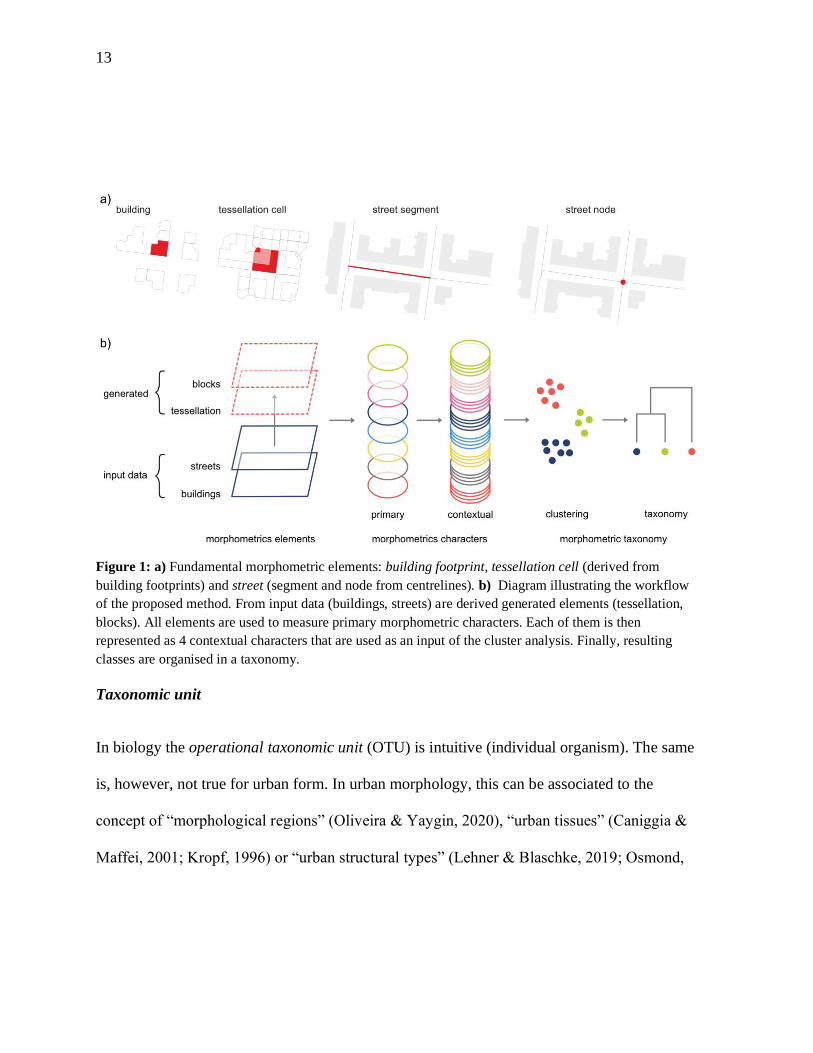
Figure 1: a) Fundamental morphometric elements: building footprint, tessellation cell (derived from

building footprints) and street (segment and node from centrelines). b) Diagram illustrating the workflow

of the proposed method. From input data (buildings, streets) are derived generated elements (tessellation,

blocks). All elements are used to measure primary morphometric characters. Each of them is then

represented as 4 contextual characters that are used as an input of the cluster analysis. Finally, resulting

classes are organised in a taxonomy.

Taxonomic unit

In biology the operational taxonomic unit (OTU) is intuitive (individual organism). The same

is, however, not true for urban form. In urban morphology, this can be associated to the

concept of “morphological regions” (Oliveira & Yaygin, 2020), “urban tissues” (Caniggia &

Maffei, 2001; Kropf, 1996) or “urban structural types” (Lehner & Blaschke, 2019; Osmond,

14

2010), or else “a distinct area of a settlement in all three dimensions, characterized by a

unique combination of streets, blocks/plot series, plots, buildings, structures and materials

and usually the result of a distinct process of formation at a particular time or period” (Kropf

2017, p.89).

From a morphometric standpoint, adopting the concept of “urban tissue” as the OTU has two

main advantages. First, being grounded on the notion of homogeneity, its definition can be

configured as a typical problem of cluster analysis: homogeneous urban tissues are hence

derived from the analysis of recurrent similarities/differences in the morphometric characters

of their constituent urban elements. Furthermore, as size and geometry of each urban tissue

are determined by internal homogeneity rather than pre-defined boundaries, the Modifiable

Aerial Unit Problem is minimised (Openshaw, 1984).

Having the elements defined, the method proposed here can be split into five consecutive

steps illustrated on figure 1b: 1) generation of morphological elements, 2) measurement of

primary morphometric characters, 3) measurement of contextual character, 4) cluster analysis,

5) taxonomy. The remaining steps are outlined in the following sections.

Morphometric characters

The definition of measurable morphometric characters is key for cluster analysis and captures

the cross-scale structural complexity of different urban tissues. To this end, building on earlier

15

literature review <masked for review>, we use six categories of morphometric characters -

dimension, shape, spatial distribution, intensity, connectivity, diversity.

These characters allow to numerically describe morphometric elements (street segments,

building footprints and tessellation cells) within any urban fabric, by capturing the

relationships between them and their immediate surroundings. They are measured at three

topological scales: small (element itself), medium (element and its immediate neighbours) and

large – the element and its neighbours within k-th order of contiguity. Spatial contiguity can

either be kept constrained by enclosing streets (the equivalent of an urban block) or left

unconstrained (see the Supplementary Material 1 for further details).

Considered morphometric characters are of two types: primary and contextual. Primary

characters measure geometric and configurational properties of morphometric elements

(buildings, streets and cells) and their relationships (at all scales). By abundantly representing

all six morphometric categories this set is extensive. Accordingly, starting from as broad a set

of unique variables identified by <masked for review>, we shortlist 74 characters (table S1 in

the Supplementary Material), following rules by Sneath & Sokal (1973) to minimise potential

collinearity and limit redundancy of information, while retaining the universality of the

method.

16

Primary characters describe morphometric elements and their immediate neighbourhood

rather than their spatial patterns. As such, when employed for cluster analysis they may result

in spatially discontinuous classes. Urban tissues are defined by their internal homogeneity, but

it can, and often is, be the homogeneity of heterogeneity. In other words, the tissue may be

defined by the combination of small and large buildings or various shapes, and we need to

capture these characteristics. Thus we derive a set of spatially lagged contextual characters

describing the tendency of each primary character in its context. The term “context” is here

defined as topological aggregation of morphological cells within three topological steps from

each given cell Ci, an empirically determined value large enough to capture a cohesive pattern

over a relatively wide spatial extent but small enough to generate sharp boundaries between

different patterns (Figure 2). The notion of “tendency” is in turn quantified through four

values:

1. Interquartile mean (IQM), the most representative value cleaned of the effect of

potential outliers.

2. Interquartile range (IQR); as local measure of statistical dispersion, describes the

range of values cleaned of outliers:

𝐼𝑄𝑅𝑐ℎ = 𝑄3𝑐ℎ − 𝑄1𝑐ℎ,

where 𝑄3𝑐ℎ and 𝑄1𝑐ℎ are is the third and quartiles of the primary character.

17

3. Interdecile Theil index (IDT), describes the local (in)equality of distribution of values:

𝐼𝐷𝑇𝑐ℎ = ∑𝑛𝑖=1 (

𝑐ℎ𝑖

∑𝑛𝑖=1 𝑐ℎ𝑖𝑙𝑛[𝑁

𝑐ℎ𝑖

∑𝑛𝑖=1 𝑐ℎ𝑖]),

where 𝑐ℎ is the primary character.

4. Simpson’s diversity index (SDI), captures the local presence of classes of values

compared to the global structure of the distribution:

𝑆𝐷𝐼𝑐ℎ =∑𝑅𝑖=1 𝑛𝑖(𝑛𝑖−1)

𝑁(𝑁−1),

where 𝑅 is richness, expressed as number of bins, 𝑛𝑖 is the number of features within i-

th bin and N is the total number of features.

Of these, the first captures the local central tendency and the latter three the distribution of

values within third order of contiguity from each cell.

Each primary character is used as an input for each contextual option. The full set of

morphometric characters hence includes 74 primary plus 296 contextual characters (74x4),

totalling 370 characters. These are computed using the bespoke open-source Python toolkit

<masked for review>, ensuring the full replicability and reproducibility of the method.

18

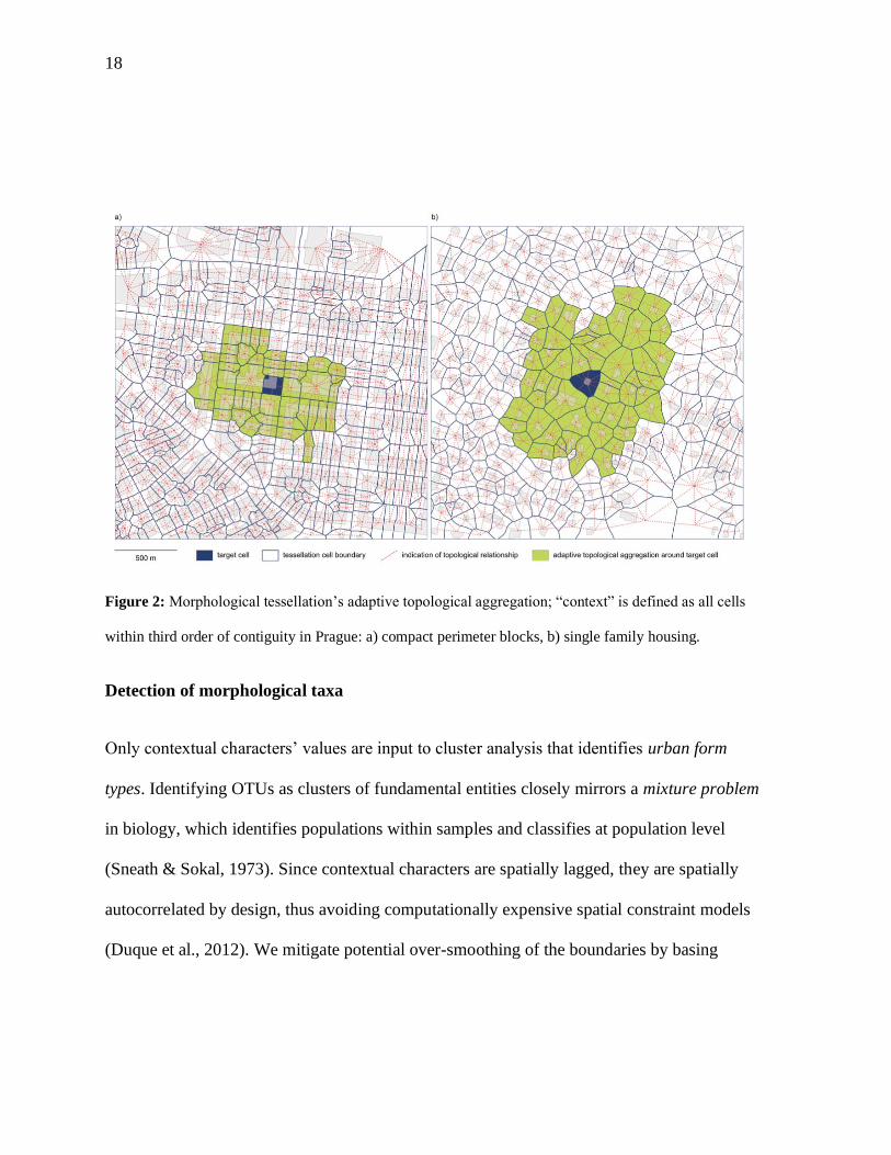
Figure 2: Morphological tessellation’s adaptive topological aggregation; “context” is defined as all cells

within third order of contiguity in Prague: a) compact perimeter blocks, b) single family housing.

Detection of morphological taxa

Only contextual characters’ values are input to cluster analysis that identifies urban form

types. Identifying OTUs as clusters of fundamental entities closely mirrors a mixture problem

in biology, which identifies populations within samples and classifies at population level

(Sneath & Sokal, 1973). Since contextual characters are spatially lagged, they are spatially

autocorrelated by design, thus avoiding computationally expensive spatial constraint models

(Duque et al., 2012). We mitigate potential over-smoothing of the boundaries by basing

19

contextual characters on truncated values (with the exception of SDI), which eliminate

outliers’ effect and define boundaries more precisely.

The most suited clustering algorithm is Gaussian Mixture Model (GMM), a probabilistic

derivative of k-means (Reynolds, 2009) tested in a similar context by Jochem et al. (2020).

Unlike the k-means itself, GMM does not rely only on squared Euclidean distances and is

more sensitive to clusters of different sizes. GMM assumes that a Gaussian distribution

represents each dimension of each cluster. Hence the cluster itself is defined by a mixture of

Gaussians. The output of GMM are cluster labels assigned to individual tessellation cells.

The ideal outcome of cluster detection would equate clusters to distinct taxa of urban tissues.

Because the definition of urban tissue (Kropf, 2017) does not specify the threshold beyond

which two similar parts of a city cluster in same tissue, it is difficult to equate clusters to taxa.

We resolve this by estimating the number of clusters, required by GMM clustering method,

on the goodness of fit of the model, measured using Bayesian Information Criterion (BIC)

(Schwarz & others, 1978) based on the “elbow” of the curve.

20

The foundation of taxonomy

To classify urban form types, we use Ward's minimum variance hierarchical clustering

previously applied in urban morphology (Dibble et al., 2019; Serra et al., 2018). Here, each

urban form type is represented by its centroid (mean of each character across cells with the

same label); Ward's algorithm links observations reducing increase in total within-cluster

variance (Ward Jr, 1963). The classification is represented through a dendrogram capturing

the cophenetic relationship between observations (i.e., morphometric similarity), forming the

foundation of our taxonomy.

Validation theory

For validation, we study our taxonomy in relation to other urban dynamics with which some

form of relation is expected. In urban morphology theory and qualitative evidence suggests

that different urban patterns emerge in areas of different historical origins or else belonging to

different “morphological periods” (Whitehand et al., 2014). This notion has also been

observed quantitatively in the urban fabric (Boeing, 2020; Dibble et al., 2019; Porta et al.,

2014, <masked>) as well as in land use patterns (Castro et al., 2019) of cities and is inherently

embedded in our OTU.

We validate our classification against three datasets: 1) historical origins; 2) predominant

land-use patterns, and 3) qualitative classification of urban form adopted in official planning

21

documents. We use the same method, based on cross-tabulation, resulting in statistical

analysis using chi-squared statistic and related Cramér’s V (Agresti, 2018). The model is

considered valid if a significant relationship is found between proposed classification and

three additional datasets and if similar performance is shown across different case studies.

Case study

We test the proposed method in two historical European cities: Prague, CZ and Amsterdam,

NL. Prague’s analysis area is defined by its administrative boundary, which extends beyond

its continuous built-up area to minimise the “edge-effect” of the street network (Gil, 2016).

Amsterdam’s analysis area is defined by its contiguous urban fabric, extending beyond the

city’s administrative boundary. The morphological data (buildings, streets) for Prague case

study were obtained from city’s open data portal (https://www.geoportalpraha.cz/en), while

the validation layers were provided by Prague Institute of Planning and Development. The

morphological data for Amsterdam are obtained from 3D BAG repository (Dukai, 2020) and

Basisregistratie Grootschalige Topografie(http://data.nlextract.nl/)

22

Results: Taxonomy of Prague and Amsterdam

We measure all 74 primary characters in both Prague and Amsterdam, associated to each

morphological cell, and subsequently generate 296 contextual characters as input to cluster

analysis.

Cluster analysis in Prague

Based on BIC results (figure S5 in the Supplementary Material), GMM clustering identifies

10 clusters (figure 3a). At a visual inspection, clusters appear well defined and able to reflect

homogenous forms, their contiguity resulting from contextual characters’ patterned nature.

23

Figure 3: Spatial distribution of detected clusters in central Prague (a) and central Amsterdam (b)

accompanied by dendrograms representing the results of Ward’s hierarchical clustering of urban form types

in Prague (c) and Amsterdam (d). The y-axis shows the cophenetic distance between individual clusters,

i.e., their morphometric dis-similarity. The full extent of case studies is shown in figures S7 and S8 in the

Supplementary Material.

24

Starting from the historical core of Prague (top left), we first identify the medieval urban form

(7), then the compact perimeter blocks of Vinohrady neighbourhood (6,), and the fringe areas

(3). Towards South and East, we note low-rise tissues (8, 1) and modernist developments (4).

Drawing purely from visual observation and personal knowledge of the city of Prague,

identified clusters appear to nicely capture meaningful urban form types.

Cluster analysis in Amsterdam

In Amsterdam, BIC indicates the optimal number being 10 clusters, similarly to Prague.

As in Prague, the geography of clusters shows seemingly meaningful results (figure 3b). For

example, cluster 7 captures the city’s historical core up to the Singelgracht canal. The cluster

1 reflects well-known shifts in planning paradigms with the rise of New Amsterdam School

(Panerai et al., 2004) forming the early 20th century south expansion. Once again, under

preliminary observation, identified clusters capture meaningful spatial patterns.

Numerical taxonomy

The centroid values of each cluster, obtained as mean value of each contextual character, are

used as taxonomic characters in Ward’s hierarchical clustering. Resulting relationship

between centroids represents relationship between clusters (figure 3c). The dendrogram’s

horizontal axis represents detected clusters, while the vertical axis their cophenetic distance

25

(i.e., morphological dissimilarity ): the lower the connecting link of two clusters, the higher

their similarity.

Prague’s dendrogram contains 10 clusters, illustrating the uniqueness of the spatial pattern of

medieval city (7), forming the first bifurcation and independent branch. The similar situation

is with cluster covering industrial areas (0) being dissimilar to other clusters. Further in the

dendrogram, we can see branches with regular perimeter blocks (6) and their fringe areas (3),

unorganised development of modern era (4, 2) or a branch featuring residential areas of low

density (9, 1, 5, 8).

The dendrogram of Amsterdam urban form (figure 3d) shows similar characteristics, with

bifurcations distinguishing nested levels of spatial variations.

In the classification maps shown in figure 3,types are colour-coded to highlight distinctions at

individual cluster’s level. However, we can instead colour-code according to clusters’

similarity. Because the dendrogram shows several major bifurcations at different levels of

cophenetic distance indicating distinct higher-order groups of clusters, by colouring each

cluster in the map according to the branch it belongs to in the dendrogram and using different

hues to distinguish between lower-level clusters in each branch, we distinguish hierarchies

based on cophenetic distance.

26

We can further combine the two cities’ clusters in one shared dendrogram (figure 4c). Urban

form types from both pools appear regularly distributed in the lowest orders of the tree,

showing a similar spatial structure emerging in both cases. Remarkably, we can see the major

bifurcation setting apart industrial urban forms in the combined taxonomy.

A lower order bifurcation within the main branch distinguishes between dense/compact urban

form and the rest. Further lower-level subdivisions are also visible. Compared to individual

ones, the combined tree shows some differences in branching: a few clusters are reshuffled

and the branches themselves are slightly reorganised. This is likely to happen as more and

more cities are analysed until the unified taxonomy reaches a “plateau” when enough cases

are included, ultimately producing a ‘general taxonomy of urban form’.

27

Figure 4: Spatial distribution of different branches of the combined dendrogram in central Prague (a) and

central Amsterdam (b) accompanied by the dendrogram representing the results of Ward’s hierarchical

clustering of urban form types from a combined pool of Prague and Amsterdam (c). The y-axis shows

cophenetic distance between individual clusters, i.e. their morphometric dis-similarity. Branches are

interpretatively coloured - the colours are then used on maps illustrating spatial distribution of these

branches. The full extent of case studies is shown in figures S9 and S10 in the Supplementary Material.

28

The geography of Prague and Amsterdam combined taxonomy (figure 4a, 4b) allows cross-

comparing urban form patterns by similarity (represented by similar colours). Same can be

extended across multitude of cities and regions.

Validation

We validate the output of numerical taxonomy against three datasets: 1) historical origins; 2)

land-use patterns, and 3) qualitative classifications. All these are assessed by contingency

table-based chi-squared statistic and Cramér's V.

In Prague, data on historical origin classifies urban areas into 7 periods: 1840, 1880, 1920,

1950, 1970, 1990, 2012, while there are 123 categories of land use at individual building/plot

level, where only 15 contain more than 1,000 buildings. We redefined prevailing land uses

within the 3 topological steps of morphological tessellation: only 5 categories (Multi-family

housing, Single-family housing, Villas, Industry small, Industry large) contain more than 1%

of the dataset. We use these five and denote the rest as Other.

Qualitative classification is drawn from a municipal typology of neighbourhoods developed

by the city for planning purposes. Each neighbourhood has specified boundaries based on its

morphology and other aspects, from historical origin to social perception and qualitatively

classified according to 10 types. We exclude 3 types, hybrid and heterogenous, which are

non-morphological and linear which captures railway structures only.

29

Differently from Prague, the Amsterdam dataset of historical origin (Dukai, 2020) indicates

each building’s year of construction, starting with 1800, rather than area/plot’s first

settlement. To ensure data compatibility with the method and avoid issues with pre-1800

periods, origin dates are binned into 11 groups following Spaan and Waag Society (2015).

The resulting chi-squared and Cramér's V values are reported in table S7. Contingency tables

are available as tables S3 – S6. All tests indicate moderate to high association between

identified clusters and the 3 sets of validation data, supporting model’s validity.

Historical origin shows moderate association in both Prague (V=0.331) and Amsterdam

(V=0.311). Because of the nature of data, where period of first development is not the only

driver of form and we have tissues – e.g. single-family – populating multiple historical

periods, a moderate association is expected. Land use (V=0.468) and municipal qualitative

classification (V=0.674), tested only in Prague, indicate moderate and high association to

clusters. Again, since land use is only a partial driver of urban form, moderate association

supports the proposed method’s potential to capture urban reality. Furthermore, relationship

between morphometric types and qualitative ones sourced from local authority is the highest

among validation data, reaching V=0.674. This seems encouraging, since both classifications

aim to capture a similar conceptualisation of the built environment.

30

Discussion

The proposed method hierarchically classifies urban form types according to the similarity of

their morphological traits. It is numerical, unsupervised, rich in information and scalable in

spatial extent. It identifies clusters of urban form as distinct urban form types and, within

each, contiguous urban tissues, reflecting that in a typical city we observe tissues belonging to

the same type. The method is parsimonious in terms of input data, requiring only building

footprints (and height) and street networks, to generate three morphometric elements

(building units, street network, morphological tessellation) and to compute the 370

morphometric characters. Such a wealth of fine-grained information allows extensively

characterising each building in the study area and its adjacency and deriving distinct urban

form types hierarchically organised according to similarity.

The method allows urban form analysis both in detail and at large scale, hence overcoming a

methodological gap; it is fully data-driven and does not rely on (but confirms) experts’

judgement other than for interpretation of BIC score. It is structurally hierarchical, which

ensures depth along the similarity structure of urban form types and flexibility of use,

according to the desired resolution of classification. Furthermore, it is extensive,

encompassing a broad range of morphometric descriptors between major urban form

31

components and their context; and it is granular, since morphometric characters are referred

to each individual building.

Finally, it is scalable and reproducible, in that it is designed to suite well the large scale of

coverage - like cities and combinations of cities - and its source code is available open-source.

Information generated with the proposed method supports applications at three different

levels. First, the set of morphometric characters can be input to studies of a relationship

between urban form and socio-economic aspects of urban life, e.g. via regression analysis.

This includes investigations into the link between urban form and energetic/bioclimatic

performance of cities, population health, gentrification and place attractiveness. Second, flat

clustering with morphometric profiles can provide aggregated information on patterns without

dealing with individual characters. This makes it possible to capture the overall morphological

“identity” of an urban tissue rather than focusing on one element at the time. Third, the

taxonomy brings hierarchy into classification and, as such, it can adapt its resolution to fit any

question asked. In this sense, while the results of the clusters may be well-suited for fine-

grained spatial analyses, by horizontally cutting the dendrogram at a desired height, it is

possible to group clusters into fewer, more generalised spatial aggregations which might be

better suited for analyses at coarser resolution.

32

Whilst parsimonious in terms of input data, our method still relies on their availability and

consistency. The building footprints layer is often of sub-optimal quality level: adjacent

buildings may be represented as unified polygons, misleading the method in dense areas.

Building-level information on height may not be available, reducing depth of information

with potentially negative effects on the quality of resulting clusters. Consistency of data

across geographies may also be an issue, particularly for large spatial extents, which may

require data generated independently by multiple sources.

Conclusions

The paper presents an original data-driven approach for the systematic unsupervised

classification and characterisation of urban form patterns grounded on numerical taxonomy in

biological systematics and which clusters urban tissues based on phenetic similarity, delivering

a systematic numerical taxonomy of urban form. More specifically it measures a selection of

74 primary characters from input data (buildings, streets) and derived generated elements

(tessellation and blocks), each of which is represented through 4 contextual characters

(Interquartile mean, Interquartile range, Interdecile Theil index, Simpson’s diversity index).

These are then used as an input of the cluster analysis, resulting in a hierarchical taxonomy.

Finally, the proposed approach is validated through two exploratory case studies illustrating

33

how the resulting clustering show significant relationship with validation data reflecting other

urban spatial dynamics.

Urban morphometrics and proposed classification method represent a step towards the

development of a taxonomy of urban form and opens to scalable urban morphology. By

overcoming existing limitations in the systematic detection and characterisation of

morphological patterns, the proposed approach opens the way to the large-scale classification

and characterisation of urban form patterns, potentially resulting, if applied to a substantial pool

of cities, in a universal taxonomy of urban form.

At the same time, the proposed approach also provides valuable tools for more rigorous

comparative studies, which are fundamental to highlight similarities and differences in urban

forms of different urban settlements in different contexts, and to explore the relationship

between urban space and phenomena as diverse as environmental performance, health and place

attractiveness and more.

34

References

● Agresti A (2018) An Introduction to Categorical Data Analysis. John Wiley & Sons.

● Angel S, Blei AM, Civco DL and Parent J (2012). Atlas of urban expansion. Lincoln

Institute of Land Policy Cambridge, MA.

● Araldi A and Fusco G (2019) From the street to the metropolitan region: Pedestrian

perspective in urban fabric analysis: Environment and Planning B: Urban Analytics

and City Science 46(7): 1243–1263. DOI: 10.1177/2399808319832612.

● Berghauser Pont M, Stavroulaki G and Marcus L (2019a) Development of urban types

based on network centrality, built density and their impact on pedestrian movement.

Environment and Planning B: Urban Analytics and City Science 46(8): 1549–1564.

DOI: 10/gghf42.

● Berghauser Pont M, Stavroulaki G, Bobkova E, et al. (2019b) The spatial distribution

and frequency of street, plot and building types across five European cities.

Environment and Planning B: Urban Analytics and City Science 46(7): 1226–1242.

DOI: 10/gf8x8j.

35

● Biljecki F, Ledoux H and Stoter J (2016) An improved LOD specification for 3D

building models. Computers, Environment and Urban Systems 59: 25–37. DOI:

10/f83fz4.

● Bobkova E, Berghauser Pont M and Marcus L (2019) Towards analytical typologies

of plot systems: Quantitative profile of five European cities. Environment and

Planning B: Urban Analytics and City Science: 239980831988090. DOI: 10/ggbgsm.

● Boeing G (2020) Off the grid… and back again? The recent evolution of american

street network planning and design. Journal of the American Planning Association.

Taylor & Francis: 1–15. DOI: 10/ghf423.

● Caniggia G and Maffei GL (2001) Architectural Composition and Building Typology:

Interpreting Basic Building. Firenze: Alinea Editrice.

● Caruso G, Hilal M and Thomas I (2017). Measuring urban forms from inter-building

distances: Combining MST graphs with a Local Index of Spatial Association.

Landscape and Urban Planning, 163, 80–89.

● Castro KB de, Roig HL, Neumann MRB, et al. (2019) New perspectives in land use

mapping based on urban morphology: A case study of the Federal District, Brazil.

Land Use Policy 87: 104032. DOI: 10.1016/j.landusepol.2019.104032.

36

● Conzen M (1960) Alnwick, Northumberland: A Study in Town-Plan Analysis. London:

George Philip & Son. Available at: http://www.jstor.org/stable/pdf/621094.pdf.

● Dibble J, Prelorendjos A, Romice O, et al. (2019) On the origin of spaces:

Morphometric foundations of urban form evolution. Environment and Planning B:

Urban Analytics and City Science 46(4): 707–730. DOI: 10.1177/2399808317725075.

● Dogrusoz E and Aksoy S (2007) Modeling urban structures using graph-based spatial

patterns. In: 1 January 2007, pp. 4826–4829. IEEE. DOI:

10.1109/IGARSS.2007.4423941.

● Dukai B (2020) 3D Registration of Buildings and Addresses (BAG) / 3D

Basisregistratie Adressen en Gebouwen (BAG). 4TU.ResearchData. DOI:

https://doi.org/10.4121/uuid:f1f9759d-024a-492a-b821-07014dd6131c.

● Duque JC, Anselin L and Rey SJ (2012) The max-p-regions problem. Journal of

Regional Science 52(3). Wiley Online Library: 397–419. DOI: 10/cf9h6h.

● Fleischmann M, Feliciotti A, Romice O, et al. (2020) Morphological tessellation as a

way of partitioning space: Improving consistency in urban morphology at the plot

37

scale. Computers, Environment and Urban Systems 80: 101441. DOI:

10.1016/j.compenvurbsys.2019.101441.

● Gil J, Beirão JN, Montenegro N, Duarte, JP (2012) On the discovery of urban

typologies: data mining the many dimensions of urban form. Urban Morphology

16(1): 27–40

● Gil J (2016) Street network analysis ‘edge effects’: Examining the sensitivity of

centrality measures to boundary conditions. Environment and Planning B: Planning

and Design. DOI: 10.1177/0265813516650678.

● Guyot M, Araldi A, Fusco G and Thomas I (2021). The urban form of Brussels from

the street perspective: The role of vegetation in the definition of the urban fabric.

Landscape and Urban Planning, 205, 103947. https://doi.org/10/ghf96c

● Hamaina R, Leduc T and Moreau G (2012) Towards Urban Fabrics Characterization

Based on Buildings Footprints. In: Bridging the Geographic Information Sciences.

Berlin, Heidelberg: Springer, Berlin, Heidelberg, pp. 327–346. DOI: 10.1007/978-3-

642-29063-3_18.

● Hartmann A, Meinel G, Hecht R, et al. (2016) A Workflow for Automatic

Quantification of Structure and Dynamic of the German Building Stock Using Official

38

Spatial Data. ISPRS International Journal of Geo-Information 5(8): 142. DOI:

10/f872vh.

● Jochem WC, Leasure DR, Pannell O, et al. (2020) Classifying settlement types from

multi-scale spatial patterns of building footprints. Environment and Planning B:

Urban Analytics and City Science: 239980832092120. DOI: 10/ggtsbn.

● Kropf K (1993) The definition of built form in urban morphology. University of

Birmingham.

● Kropf K (1996) Urban tissue and the character of towns. URBAN DESIGN

International 1(3): 247–263. DOI: 10.1057/udi.1996.32.

● Kropf K (2014) Ambiguity in the definition of built form. Urban Morphology 18(1):

41–57.

● Kropf K (2017) The Handbook of Urban Morphology. Chichester: John Wiley &

Sons. Available at: http://cds.cern.ch/record/2316422.

● Kropf K (2018) Plots, property and behaviour. Urban Morphology 22(1): 5–14.

● Lehner A and Blaschke T (2019) A Generic Classification Scheme for Urban

Structure Types. Remote Sensing 11(2): 173. DOI: 10.3390/rs11020173.

39

● Levy A (1999) Urban morphology and the problem of the modern urban fabric: some

questions for research. Urban Morphology 3: 79–85.

● Louf R and Barthelemy M (2014) A typology of street patterns. Journal of the Royal

Society Interface 11. DOI: http://dx.doi.org/10.1098/rsif.2014.0924.

● Moudon AV (1997) Urban morphology as an emerging interdisciplinary field. Urban

Morphology 1(1): 3–10.

● Muratori S (1959) Studi per una operante storia urbana di Venezia. Palladio. Rivista di

storia dell’architettura 1959: 1–113.

● Neidhart H and Sester M (2004) Identifying building types and building clusters using

3-D laser scanning and GIS-data. Int Arch Photogramm Remote Sens Spatial Inf Sci

35: 715–720.

● Oliveira V (2016) Urban Morphology: An Introduction to the Study of the Physical

Form of Cities. Cham: Springer International Publishing.

● Oliveira V and Yaygin MA (2020) The concept of the morphological region:

developments and prospects. Urban Morphology 24(1): 18.

● Openshaw S (1984) The Modifiable Areal Unit Problem.

40

● Osmond P (2010) The urban structural unit: Towards a descriptive framework to

support urban analysis and planning. Urban Morphology 14(1): 5–20.

● Porta S, Romice O, Maxwell JA, et al. (2014) Alterations in scale: Patterns of change

in main street networks across time and space. Urban Studies 51(16): 3383–3400.

DOI: 10.1177/0042098013519833.

● Reynolds DA (2009) Gaussian mixture models. Encyclopedia of biometrics 741.

Berlin, Springer. DOI: 10/cqtzqm.

● Schirmer PM and Axhausen KW (2015) A multiscale classification of urban

morphology. Journal of Transport and Land Use 9(1): 101–130. DOI:

10.5198/jtlu.2015.667.

● Schwarz G and others (1978) Estimating the dimension of a model. The annals of

statistics 6(2). Institute of Mathematical Statistics: 461–464.

● Serra M, Psarra S and O’Brien J (2018) Social and Physical Characterization of Urban

Contexts: Techniques and Methods for Quantification, Classification and Purposive

Sampling. Urban Planning 3(1): 58–74. DOI: 10.17645/up.v3i1.1269.

● Sneath PHA and Sokal RR (1973) Numerical Taxonomy. San Francisco: Freeman.

41

● Soman S, Beukes A, Nederhood C, Marchio N and Bettencourt L (2020). Worldwide

detection of informal settlements via topological analysis of crowdsourced digital

maps. ISPRS International Journal of Geo-Information, 9(11), 685.

https://doi.org/10/ghpwqm

● Song Y and Knaap G-J (2007) Quantitative Classification of Neighbourhoods: The

Neighbourhoods of New Single-family Homes in the Portland Metropolitan Area.

Journal of Urban Design 12(1): 1–24. DOI: 10.1080/13574800601072640.

● Spaan B and Waag Society (2015) All buildings in Netherlands shaded by a year of

construction. Available at: https://code.waag.org/buildings/.

● Steadman, P. (1979). The Evolution of Designs Biological Analogy in Architecture

and the Applied Arts.

● Steiniger S, Lange T, Burghardt D, et al. (2008) An Approach for the Classification of

Urban Building Structures Based on Discriminant Analysis Techniques. Transactions

in GIS 12(1): 31–59. DOI: 10.1111/j.1467-9671.2008.01085.x.

● Stewart ID and Oke TR (2012) Local Climate Zones for Urban Temperature Studies.

Bulletin of the American Meteorological Society 93(12): 1879–1900. DOI:

10.1175/BAMS-D-11-00019.1.

42

● Taubenböck H, Debray H, Qiu C, et al. (2020) Seven city types representing

morphologic configurations of cities across the globe. Cities 105: 102814. DOI:

10/gg2jv4.

● Usui H and Asami Y (2013) Estimation of Mean Lot Depth and Its Accuracy. Journal

of the City Planning Institute of Japan 48(3): 357–362.

● Ward Jr JH (1963) Hierarchical grouping to optimize an objective function. Journal of

the American statistical association 58(301). Taylor & Francis Group: 236–244. DOI:

10/fz95kg.

● Whitehand J, Gu K, Conzen MP, et al. (2014) The typological process and the

morphological period: a cross-cultural assessment. Environment and Planning B:

Planning and Design 41(3). SAGE Publications Sage UK: London, England: 512–

533. DOI: 10/f546ck.

● Wurm M, Schmitt A and Taubenbock H (2016) Building Types’ Classification Using

Shape-Based Features and Linear Discriminant Functions. IEEE Journal of Selected

Topics in Applied Earth Observations and Remote Sensing 9(5): 1901–1912. DOI:

10.1109/JSTARS.2015.2465131.

43

Supplementary material

Supplementary Material 1: Relational analytical framework

This research proposes and applies a relational framework of urban form for urban

morphometrics.

Relational analytical framework (RF) of urban form is based on two concepts - topology and

inclusiveness. The framework acknowledges that there are identifiable relations between all

elements of urban form and their aggregations. As such, it accommodates all analytical

aggregations into a singular framework, linking all potential measurable characters to the

smallest element. Furthermore, it employs topological relations in the way it generates

location-based aggregations of fundamental elements.

Unlike existing frameworks in literature, RF is analytical, not conceptual or structural. It does

not try to propose a new theory of urban form; it has purely morphometric nature.

Within this research, RF is operationalised based on morphological tessellation.

The key principles of the tessellation-based relation framework are as follows.

1. Urban form is represented as building footprints, street networks and footprint-based

morphological tessellation.

2. There is an identifiable relationship between buildings and street networks, buildings and

street nodes and buildings and tessellation cells.

3. Morphometric characters are measured on scales defined by topological relations between

elements.

- Element itself

- Element and its immediate neighbours

- Element and its neighbours within n topological steps, either in a constrained or an

unconstrained way.

4. Therefore, we can define subsets of RF as measurable entities of urban form based on

fundamental elements and topological scales.

5. Subsets are overlapping, reusing each element within all relevant relations.

Since the relation between all elements is preserved throughout the process of their

combination, we can always link values measured on one subset to another. For example, due

to the fixed relation between building and street node, we can attach a node's degree value to a

44

building as an element. The constrained topological relation can identify traditional area-

based aggregations like block (as a combination of all tessellation cells which topological

relation does not cross a street). As such, they allow us to combine both area-based and

location-based aggregations while minimising MAUP for each of them.

Subsets of elements

Subsets are a combination of topological scales and fundamental elements. Overlap of

morphometric characters derived from subsets, where each subset is representing a different

structural unit, gives an overall characteristic of each duality building - cell, which can be

later used for further analysis.

We can divide subsets into three topological scales: Small (or Single), Medium and Large.

Note that topological distance is possible to define within each layer (relations between

buildings, relations between cells, relations between edges or nodes), but not as a combination

of layers. The relation between building, its cell, its segment and its node is fixed and seen as

a singular feature. That is why morphometric characters like covered area ratio of the cell are

classified as a Small scale character.

Small/Single (S)

Small scale captures fundamental elements themselves (topological distance is 0 - itself). In

the case of building and tessellation cell, it captures the individual character of each cell. In

the case of street segment and node, it captures value for segment or node, which is then

applied to each cell attached to it.

We have four subsets within small scale:

- building

- tessellation cell

- street segment

- street node

45

Figure S1: Diagrams illustrating the subsets on the small/single scale.

Medium (M)

The medium scale reflects topological distance 1. It captures individual character for each

element derived from the relation to its adjacent elements.

- adjacent buildings

- neighbouring cells

- neighbouring segments

- linked nodes

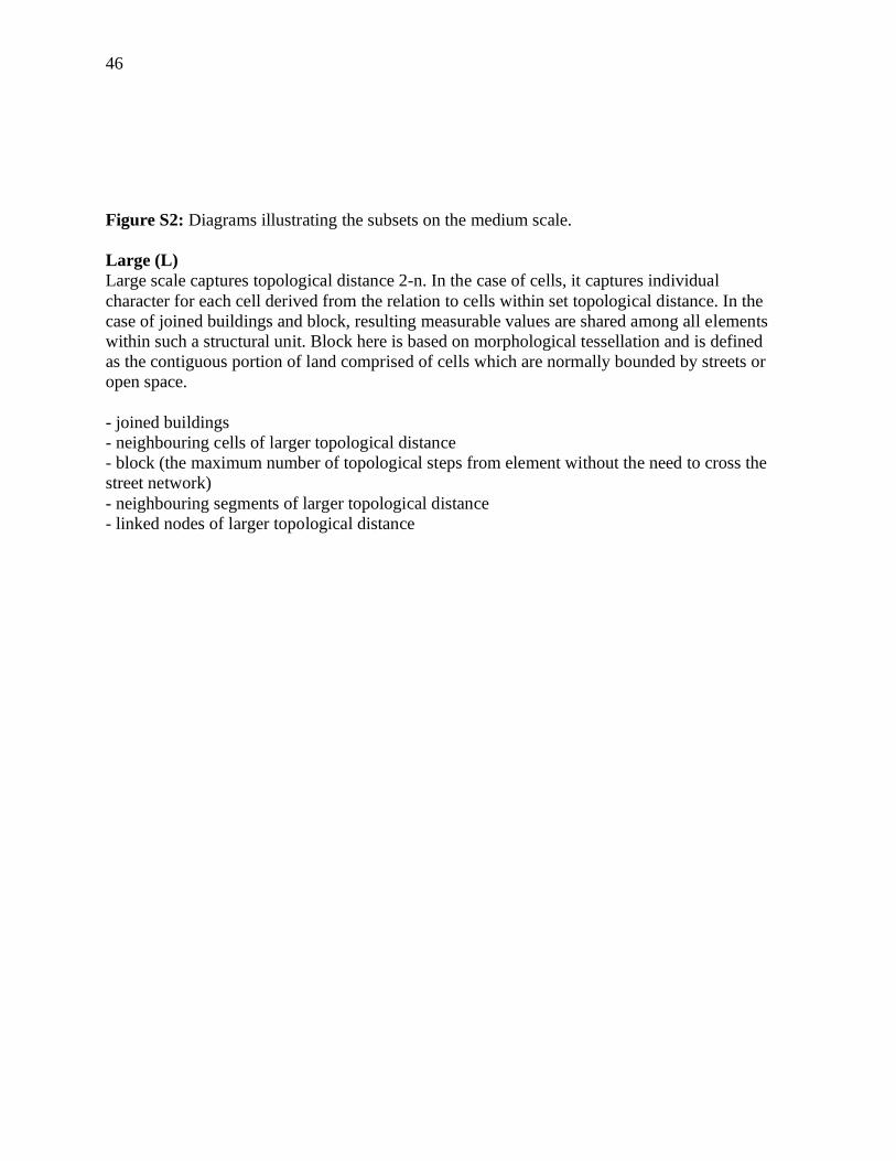
46

Figure S2: Diagrams illustrating the subsets on the medium scale.

Large (L)

Large scale captures topological distance 2-n. In the case of cells, it captures individual

character for each cell derived from the relation to cells within set topological distance. In the

case of joined buildings and block, resulting measurable values are shared among all elements

within such a structural unit. Block here is based on morphological tessellation and is defined

as the contiguous portion of land comprised of cells which are normally bounded by streets or

open space.

- joined buildings

- neighbouring cells of larger topological distance

- block (the maximum number of topological steps from element without the need to cross the

street network)

- neighbouring segments of larger topological distance

- linked nodes of larger topological distance

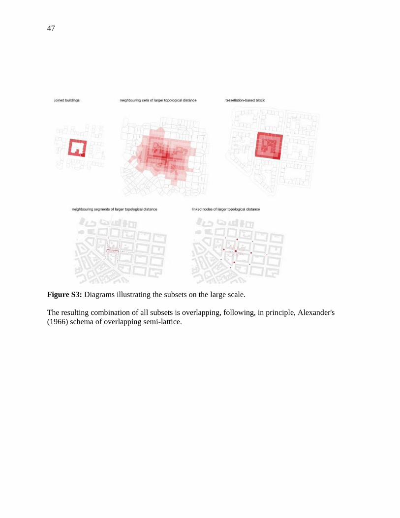
47

Figure S3: Diagrams illustrating the subsets on the large scale.

The resulting combination of all subsets is overlapping, following, in principle, Alexander's

(1966) schema of overlapping semi-lattice.

48

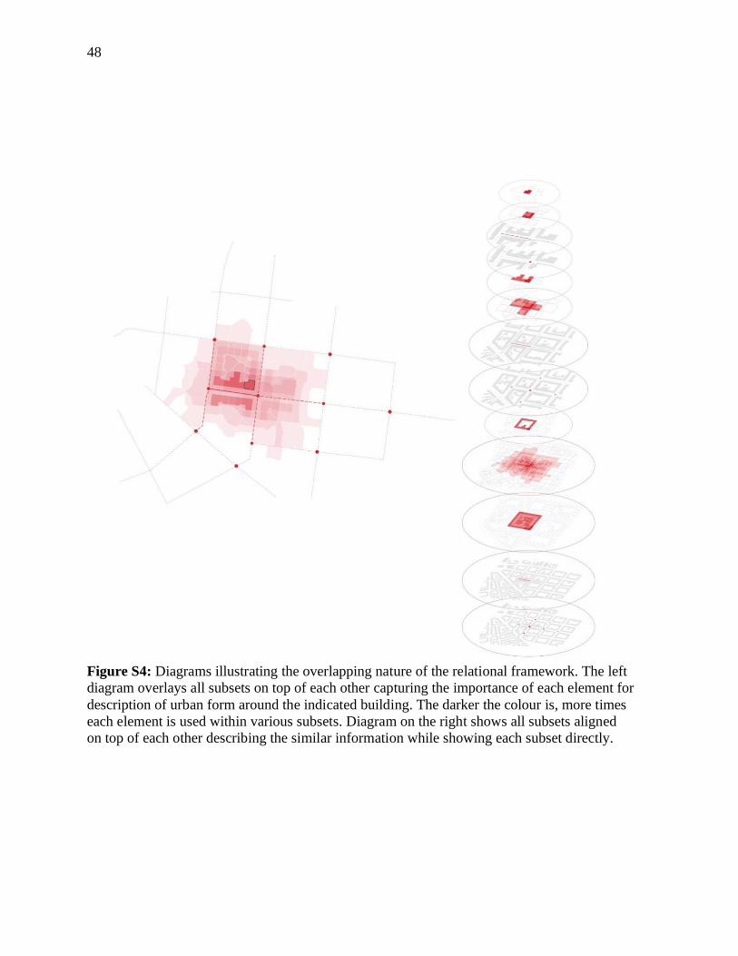
Figure S4: Diagrams illustrating the overlapping nature of the relational framework. The left

diagram overlays all subsets on top of each other capturing the importance of each element for

description of urban form around the indicated building. The darker the colour is, more times

each element is used within various subsets. Diagram on the right shows all subsets aligned

on top of each other describing the similar information while showing each subset directly.

49

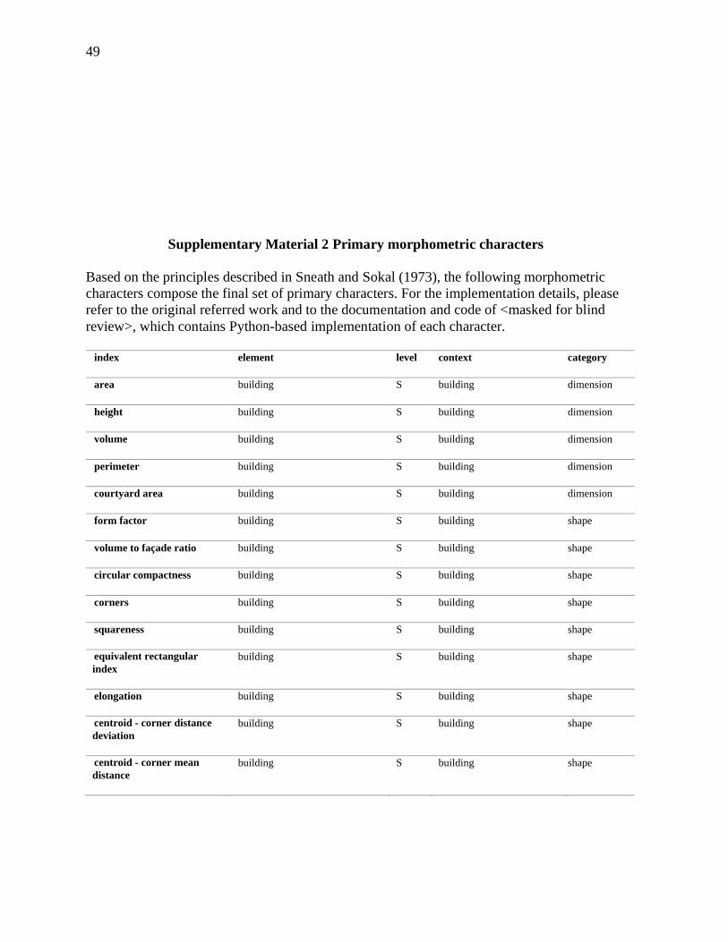
Supplementary Material 2 Primary morphometric characters

Based on the principles described in Sneath and Sokal (1973), the following morphometric

characters compose the final set of primary characters. For the implementation details, please

refer to the original referred work and to the documentation and code of <masked for blind

review>, which contains Python-based implementation of each character.

index element level context category

area building S building dimension

height building S building dimension

volume building S building dimension

perimeter building S building dimension

courtyard area building S building dimension

form factor building S building shape

volume to façade ratio building S building shape

circular compactness building S building shape

corners building S building shape

squareness building S building shape

equivalent rectangular

index

building S building shape

elongation building S building shape

centroid - corner distance

deviation

building S building shape

centroid - corner mean

distance

building S building shape

50

solar orientation building S building distribution

street alignment building S building distribution

cell alignment building S building distribution

longest axis length tessellation cell S tessellation cell dimension

area tessellation cell S tessellation cell dimension

circular compactness tessellation cell S tessellation cell shape

zequivalent rectangular

index

tessellation cell S tessellation cell shape

solar orientation tessellation cell S tessellation cell distribution

street alignment tessellation cell S tessellation cell distribution

coverage area ratio tessellation cell S tessellation cell intensity

floor area ratio tessellation cell S tessellation cell intensity

length street segment S street segment dimension

width street profile S street segment dimension

height street profile S street segment dimension

height to width ratio street profile S street segment shape

openness street profile S street segment distribution

width deviation street profile S street segment diversity

height deviation street profile S street segment diversity

linearity street segment S street segment shape

area covered street segment S street segment dimension

buildings per meter street segment S street segment intensity

area covered street node S street node dimension

51

shared walls ratio adjacent buildings M adjacent buildings distribution

alignment neighbouring buildings M neighbouring cells (queen) distribution

mean distance neighbouring buildings M neighbouring cells (queen) distribution

weighted neighbours tessellation cell M neighbouring cells (queen) distribution

area covered neighbouring cells M neighbouring cells (queen) dimension

reached cells neighbouring segments M neighbouring segments intensity

reached area neighbouring segments M neighbouring segments dimension

degree street node M neighbouring nodes distribution

mean distance to

neighbouring nodes

street node M neighbouring nodes dimension

reached cells neighbouring nodes M neighbouring nodes intensity

reached area neighbouring nodes M neighbouring nodes dimension

number of courtyards adjacent buildings L joined buildings intensity

perimeter wall length adjacent buildings L joined buildings dimension

mean inter-building

distance

neighbouring buildings L cell queen neighbours 3 distribution

building adjacency neighbouring buildings L cell queen neighbours 3 distribution

gross floor area ratio neighbouring tessellation cells L cell queen neighbours 3 intensity

weighted reached blocks neighbouring tessellation cells L cell queen neighbours 3 intensity

area block L block dimension

perimeter block L block dimension

circular compactness block L block shape

equivalent rectangular

index

block L block shape

52

compactness-weighted axis block L block shape

solar orientation block L block distribution

weighted neighbours block L block distribution

weighted cells block L block intensity

local meshedness street network L nodes 5 steps connectivity

mean segment length street network L segment 3 steps dimension

cul-de-sac length street network L nodes 3 steps dimension

reached cells street network L segment 3 steps dimension

node density street network L nodes 5 steps intensity

reached cells street network L nodes 3 steps dimension

reached area street network L nodes 3 steps dimension

proportion of cul-de-sacs street network L nodes 5 steps connectivity

proportion of 3-way

intersections

street network L nodes 5 steps connectivity

proportion of 4-way

intersections

street network L nodes 5 steps connectivity

weighted node density street network L

intensity

local closeness centrality street network L nodes 5 steps connectivity

square clustering street network L nodes within network connectivity

Table S1: Table of primary morphometric characters. For detailed explanation, formulas and

references, see the details below. Nomenclature follows the Index of Element model proposed

by <masked for blind review>. Scale refers to the topological scale from which a character is

derived, while context describes the actual set of elements used.

53

1. Area of a building is denoted as

𝑎𝑏𝑙𝑔

and defined as an area covered by a building footprint in m2.

2. Height of a building is denoted as

ℎ𝑏𝑙𝑔

and defined as building height in m measured optimally as weighted mean height (in case of

buildings with multiple parts of different height). It is a required input value not measured

within the morphometric assessment itself.

3. Volume of a building is denoted as

𝑣𝑏𝑙𝑔 = 𝑎𝑏𝑙𝑔 × ℎ𝑏𝑙𝑔

and defined as building footprint multiplied by its height in m3.

4. Perimeter of a building is denoted as

𝑝𝑏𝑙𝑔

and defined as the sum of lengths of the building exterior walls in m.

5. Courtyard area of a building is denoted as

𝑎𝑏𝑙𝑔𝑐

and defined as the sum of areas of interior holes in footprint polygons in m2.

6. Form factor of a building is denoted as

𝐹𝑜𝐹𝑏𝑙𝑔 =𝑎𝑏𝑙𝑔

𝑣𝑏𝑙𝑔

23

.

It captures three-dimensional unitless shape characteristic of a building envelope unbiased by

the building size (Bourdic et al., 2012).

7. Volume to façade ratio of a building is denoted as

𝑉𝐹𝑅𝑏𝑙𝑔 =𝑣𝑏𝑙𝑔

𝑝𝑏𝑙𝑔×ℎ𝑏𝑙𝑔.

54

It captures the aspect of the three-dimensional shape of a building envelope able to distinguish

building types, as shown by Schirmer and Axhausen (2015). It can be seen as a proxy of

volumetric compactness.

8. Circular compactness of a building is denoted as

𝐶𝐶𝑜𝑏𝑙𝑔 =𝑎𝑏𝑙𝑔𝑎𝑏𝑙𝑔𝐶

where 𝑎𝑏𝑙𝑔𝐶 is an area of minimal enclosing circle. It captures the relation of building

footprint shape to its minimal enclosing circle, illustrating the similarity of shape and circle

(Dibble et al., 2019).

9. Corners of a building is denoted as

𝐶𝑜𝑟𝑏𝑙𝑔 = ∑

𝑛

𝑖=1

𝑐𝑏𝑙𝑔

where 𝑐𝑏𝑙𝑔 is defined as a vertex of building exterior shape with an angle between adjacent

line segments ≤ 170 degrees. It uses only external shape, courtyards are not included.

Character is adapted from Steiniger et al. (2008) to exclude non-corner-like vertices.

10. Squareness of a building is denoted as

𝑆𝑞𝑢𝑏𝑙𝑔 =∑𝑛𝑖=1 𝐷𝑐𝑏𝑙𝑔𝑖

𝑛

where 𝐷 is the deviation of angle of corner 𝑐𝑏𝑙𝑔𝑖 from 90 degrees and 𝑛 is a number of

corners.

11. Equivalent rectangular index of a building is denoted as

𝐸𝑅𝐼𝑏𝑙𝑔 = √𝑎𝑏𝑙𝑔𝑎𝑏𝑙𝑔𝐵

∗𝑝𝑏𝑙𝑔𝐵𝑝𝑏𝑙𝑔

where 𝑎𝑏𝑙𝑔𝐵 is an area of a minimal rotated bounding rectangle of a building (MBR) footprint

and 𝑝𝑏𝑙𝑔𝐵 its perimeter of MBR. It is a measure of shape complexity identified by Basaraner

and Cetinkaya (2017) as the shape characters with the best performance.

12. Elongation of a building is denoted as

55

𝐸𝑙𝑜𝑏𝑙𝑔 =𝑙𝑏𝑙𝑔𝐵𝑤𝑏𝑙𝑔𝐵

where 𝑙𝑏𝑙𝑔𝐵 is length of MBR and 𝑤𝑏𝑙𝑔𝐵 is width of MBR. It captures the ratio of shorter to

the longer dimension of MBR to indirectly capture the deviation of the shape from a square

(Schirmer and Axhausen, 2015).

13. Centroid - corner distance deviation of a building is denoted as

𝐶𝐶𝐷𝑏𝑙𝑔 = √1

𝑛∑

𝑛

𝑖=1

(𝑐𝑐𝑑𝑖 − 𝑐𝑐𝑑‾)2

where 𝑐𝑐𝑑𝑖 is a distance between centroid and corner 𝑖 and 𝑐𝑐𝑑‾ is mean of all distances. It

captures a variety of shape. As a corner is considered vertex with angle < 170º to reflect

potential circularity of object and topological imprecision of building polygon.

14. Centroid - corner mean distance of a building is denoted as

𝐶𝐶𝑀𝑏𝑙𝑔 =1

𝑛(∑

𝑛

𝑖=1

𝑐𝑐𝑑𝑖)

where 𝑐𝑐𝑑𝑖 is a distance between centroid and corner 𝑖. It is a character measuring a

dimension of the object dependent on its shape (Schirmer and Axhausen, 2015).

15. Solar orientation of a building is denoted as

𝑂𝑟𝑖𝑏𝑙𝑔 = |𝑜𝑏𝑙𝑔𝐵 − 45|

where 𝑜𝑏𝑙𝑔𝐵 is an orientation of the longest axis of bounding rectangle in a range 0 - 45. It

captures the deviation of orientation from cardinal directions. There are multiple ways of

capturing orientation of a polygon. As reported by Yan et al. (2007), Duchêne et al. (2003)

assessed five different options (longest edge, weighted bisector, wall average, statistical

weighting, bounding rectangle) and concluded a bounding rectangle as the most appropriate.

Deviation from cardinal directions is used to avoid sudden changes between square-like

objects.

16. Street alignment of a building is denoted as

𝑆𝐴𝑙𝑏𝑙𝑔 = |𝑂𝑟𝑖𝑏𝑙𝑔 − 𝑂𝑟𝑖𝑒𝑑𝑔|

56

where 𝑂𝑟𝑖𝑏𝑙𝑔 is a solar orientation of the building and 𝑂𝑟𝑖𝑒𝑑𝑔 is a solar orientation of the

street edge. It reflects the relationship between the building and its street, whether it is facing

the street directly or indirectly (Schirmer and Axhausen, 2015).

17. Cell alignment of a building is denoted as

𝐶𝐴𝑙𝑏𝑙𝑔 = |𝑂𝑟𝑖𝑏𝑙𝑔 −𝑂𝑟𝑖𝑐𝑒𝑙𝑙|

where 𝑂𝑟𝑖𝑐𝑒𝑙𝑙 is a solar orientation of tessellation cell. It reflects the relationship between a

building and its cell.

18. Longest axis length of a tessellation cell is denoted as

𝐿𝐴𝐿𝑐𝑒𝑙𝑙 = 𝑑𝑐𝑒𝑙𝑙𝐶

where 𝑑𝑐𝑒𝑙𝑙𝐶 is a diameter of the minimal circumscribed circle around the tessellation cell

polygon. The axis itself does not have to be fully within the polygon. It could be seen as a

proxy of plot depth for tessellation-based analysis.

19. Area of a tessellation cell is denoted as

𝑎𝑐𝑒𝑙𝑙

and defined as an area covered by a tessellation cell footprint in m2.

20. Circular compactness of a tessellation cell is denoted as

𝐶𝐶𝑜𝑐𝑒𝑙𝑙 =𝑎𝑐𝑒𝑙𝑙𝑎𝑐𝑒𝑙𝑙𝐶

where 𝑎𝑐𝑒𝑙𝑙𝐶 is an area of minimal enclosing circle. It captures the relation of tessellation cell

footprint shape to its minimal enclosing circle, illustrating the similarity of shape and circle.

21. Equivalent rectangular index of a tessellation cell is denoted as

𝐸𝑅𝐼𝑐𝑒𝑙𝑙 = √𝑎𝑐𝑒𝑙𝑙𝑎𝑐𝑒𝑙𝑙𝐵

∗𝑝𝑐𝑒𝑙𝑙𝐵𝑝𝑐𝑒𝑙𝑙

where 𝑎𝑐𝑒𝑙𝑙𝐵 is an area of the minimal rotated bounding rectangle of a tessellation cell (MBR)

footprint and 𝑝𝑐𝑒𝑙𝑙𝐵 its perimeter of MBR.

22. Solar orientation of a tessellation cell is denoted as

𝑂𝑟𝑖𝑐𝑒𝑙𝑙 = |𝑜𝑐𝑒𝑙𝑙𝐵 − 45|

57

where 𝑜𝑐𝑒𝑙𝑙𝐵 is an orientation of the longest axis of bounding rectangle in a range 0 - 45. It

captures the deviation of orientation from cardinal directions.

23. Street alignment of a building is denoted as

𝑆𝐴𝑙𝑐𝑒𝑙𝑙 = |𝑂𝑟𝑖𝑐𝑒𝑙𝑙 − 𝑂𝑟𝑖𝑒𝑑𝑔|

where 𝑂𝑟𝑖𝑐𝑒𝑙𝑙 is a solar orientation of tessellation cell and 𝑂𝑟𝑖𝑒𝑑𝑔 is a solar orientation of the

street edge. It reflects the relationship between tessellation cell and its street, whether it is

facing the street directly or indirectly.

24. Coverage area ratio of a tessellation cell is denoted as

𝐶𝐴𝑅𝑐𝑒𝑙𝑙 =𝑎𝑏𝑙𝑔𝑎𝑐𝑒𝑙𝑙

where 𝑎𝑏𝑙𝑔 is an area of a building and 𝑎𝑐𝑒𝑙𝑙 is an area of related tessellation cell (Schirmer

and Axhausen, 2015). Coverage area ratio (CAR) is one of the commonly used characters

capturing intensity of development. However, the definitions vary based on the spatial unit.

25. Floor area ratio of a tessellation cell is denoted as

𝐹𝐴𝑅𝑐𝑒𝑙𝑙 =𝑓𝑎𝑏𝑙𝑔𝑎𝑐𝑒𝑙𝑙

where 𝑓𝑎𝑏𝑙𝑔 is a floor area of a building and 𝑎𝑐𝑒𝑙𝑙 is an area of related tessellation cell. Floor

area could be computed based on the number of levels or using an approximation based on

building height.

26. Length of a street segment is denoted as

𝑙𝑒𝑑𝑔

and defined as a length of a LineString geometry in metres.

27. Width of a street profile is denoted as

𝑤𝑠𝑝 =1

𝑛(∑

𝑛

𝑖=1

𝑤𝑖)

where 𝑤𝑖 is width of a street section i. The algorithm generates street sections every 3 meters

alongside the street segment, and measures mean value. In the case of the open-ended street,

50 metres is used as a perception-based proximity limit (Araldi and Fusco, 2019).

58

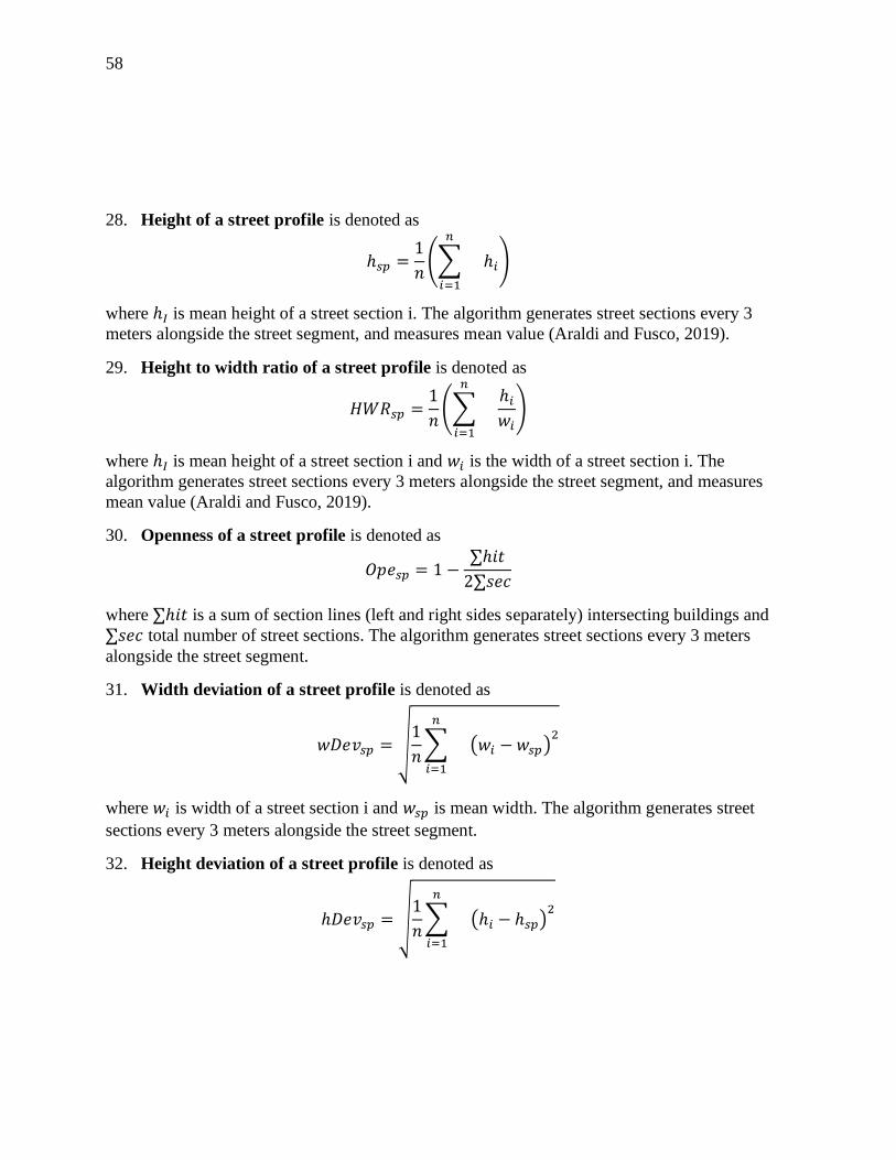
28. Height of a street profile is denoted as

ℎ𝑠𝑝 =1

𝑛(∑

𝑛

𝑖=1

ℎ𝑖)

where ℎ𝐼 is mean height of a street section i. The algorithm generates street sections every 3

meters alongside the street segment, and measures mean value (Araldi and Fusco, 2019).

29. Height to width ratio of a street profile is denoted as

𝐻𝑊𝑅𝑠𝑝 =1

𝑛(∑

𝑛

𝑖=1

ℎ𝑖𝑤𝑖)

where ℎ𝐼 is mean height of a street section i and 𝑤𝑖 is the width of a street section i. The

algorithm generates street sections every 3 meters alongside the street segment, and measures

mean value (Araldi and Fusco, 2019).

30. Openness of a street profile is denoted as

𝑂𝑝𝑒𝑠𝑝 = 1 −∑ℎ𝑖𝑡

2∑𝑠𝑒𝑐

where ∑ℎ𝑖𝑡 is a sum of section lines (left and right sides separately) intersecting buildings and

∑𝑠𝑒𝑐 total number of street sections. The algorithm generates street sections every 3 meters

alongside the street segment.

31. Width deviation of a street profile is denoted as

𝑤𝐷𝑒𝑣𝑠𝑝 = √1

𝑛∑

𝑛

𝑖=1

(𝑤𝑖 −𝑤𝑠𝑝)2

where 𝑤𝑖 is width of a street section i and 𝑤𝑠𝑝 is mean width. The algorithm generates street

sections every 3 meters alongside the street segment.

32. Height deviation of a street profile is denoted as

ℎ𝐷𝑒𝑣𝑠𝑝 = √1

𝑛∑

𝑛

𝑖=1

(ℎ𝑖 − ℎ𝑠𝑝)2

59

where ℎ𝑖 is height of a street section i and ℎ𝑠𝑝 is mean height. The algorithm generates street

sections every 3 meters alongside the street segment.

33. Linearity of a street segment is denoted as

𝐿𝑖𝑛𝑒𝑑𝑔 =𝑙𝑒𝑢𝑐𝑙𝑙𝑒𝑑𝑔

where 𝑙𝑒𝑢𝑐𝑙 is Euclidean distance between endpoints of a street segment and 𝑙𝑒𝑑𝑔 is a street

segment length. It captures the deviation of a segment shape from a straight line. It is adapted

from (Araldi and Fusco, 2019).

34. Area covered by a street segment is denoted as

𝑎𝑒𝑑𝑔 =∑

𝑛

𝑖=1

𝑎𝑐𝑒𝑙𝑙𝑖

where 𝑎𝑐𝑒𝑙𝑙𝑖 is an area of tessellation cell 𝑖 belonging to the street segment. It captures the area

which is likely served by each segment.

35. Buildings per meter of a street segment is denoted as

𝐵𝑝𝑀𝑒𝑑𝑔 =∑𝑏𝑙𝑔

𝑙𝑒𝑑𝑔

where ∑𝑏𝑙𝑔 is a number of buildings belonging to a street segment and 𝑙𝑒𝑑𝑔 is a length of a

street segment. It reflects the granularity of development along each segment.

36. Area covered by a street node is denoted as

𝑎𝑛𝑜𝑑𝑒 =∑

𝑛

𝑖=1

𝑎𝑐𝑒𝑙𝑙𝑖

where 𝑎𝑐𝑒𝑙𝑙𝑖 is an area of tessellation cell 𝑖 belonging to the street node. It captures the area

which is likely served by each node.

37. Shared walls ratio of adjacent buildings is denoted as

𝑆𝑊𝑅𝑏𝑙𝑔 =𝑝𝑏𝑙𝑔𝑠ℎ𝑎𝑟𝑒𝑑𝑝𝑏𝑙𝑔

60

where 𝑝𝑏𝑙𝑔𝑠ℎ𝑎𝑟𝑒𝑑 is a length of a perimeter shared with adjacent buildings and 𝑝𝑏𝑙𝑔 is a

perimeter of a building. It captures the amount of wall space facing the open space (Hamaina

et al., 2012).

38. Alignment of neighbouring buildings is denoted as

𝐴𝑙𝑖𝑏𝑙𝑔 =1

𝑛∑

𝑛

𝑖=1

|𝑂𝑟𝑖𝑏𝑙𝑔 − 𝑂𝑟𝑖𝑏𝑙𝑔𝑖|

where 𝑂𝑟𝑖𝑏𝑙𝑔 is the solar orientation of a building and 𝑂𝑟𝑖𝑏𝑙𝑔𝑖 is the solar orientation of

building 𝑖 on a neighbouring tessellation cell. It calculates the mean deviation of solar

orientation of buildings on adjacent cells from a building. It is adapted from Hijazi et al.

(2016).

39. Mean distance to neighbouring buildings is denoted as

𝑁𝐷𝑖𝑏𝑙𝑔 =1

𝑛∑

𝑛

𝑖=1

𝑑𝑏𝑙𝑔,𝑏𝑙𝑔𝑖

where 𝑑𝑏𝑙𝑔,𝑏𝑙𝑔𝑖 is a distance between building and building 𝑖 on a neighbouring tessellation

cell. It is adapted from Hijazi et al. (2016). It captures the average proximity to other

buildings.

40. Weighted neighbours of a tessellation cell is denoted as

𝑊𝑁𝑒𝑐𝑒𝑙𝑙 =∑𝑐𝑒𝑙𝑙𝑛𝑝𝑐𝑒𝑙𝑙

where ∑𝑐𝑒𝑙𝑙𝑛 is a number of cell neighbours and 𝑝𝑐𝑒𝑙𝑙 is a perimeter of a cell. It reflects

granularity of morphological tessellation.

41. Area covered by neighbouring cells is denoted as

𝑎𝑐𝑒𝑙𝑙𝑛 =∑

𝑛

𝑖=1

𝑎𝑐𝑒𝑙𝑙𝑖

where 𝑎𝑐𝑒𝑙𝑙𝑖 is area of tessellation cell 𝑖 within topological distance 1. It captures the scale of

morphological tessellation.

42. Reached cells by neighbouring segments is denoted as

61

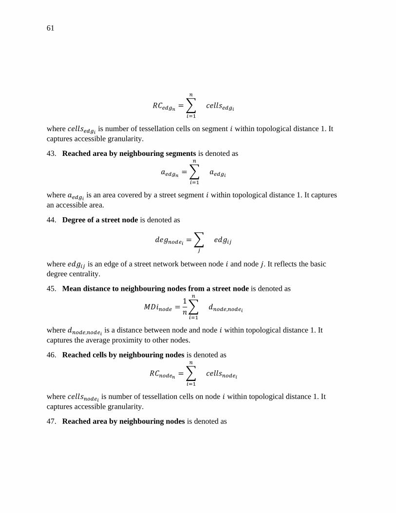
𝑅𝐶𝑒𝑑𝑔𝑛 =∑

𝑛

𝑖=1

𝑐𝑒𝑙𝑙𝑠𝑒𝑑𝑔𝑖

where 𝑐𝑒𝑙𝑙𝑠𝑒𝑑𝑔𝑖 is number of tessellation cells on segment 𝑖 within topological distance 1. It

captures accessible granularity.

43. Reached area by neighbouring segments is denoted as

𝑎𝑒𝑑𝑔𝑛 =∑

𝑛

𝑖=1

𝑎𝑒𝑑𝑔𝑖

where 𝑎𝑒𝑑𝑔𝑖 is an area covered by a street segment 𝑖 within topological distance 1. It captures

an accessible area.

44. Degree of a street node is denoted as

𝑑𝑒𝑔𝑛𝑜𝑑𝑒𝑖 =∑

𝑗

𝑒𝑑𝑔𝑖𝑗

where 𝑒𝑑𝑔𝑖𝑗 is an edge of a street network between node 𝑖 and node 𝑗. It reflects the basic

degree centrality.

45. Mean distance to neighbouring nodes from a street node is denoted as

𝑀𝐷𝑖𝑛𝑜𝑑𝑒 =1

𝑛∑

𝑛

𝑖=1

𝑑𝑛𝑜𝑑𝑒,𝑛𝑜𝑑𝑒𝑖

where 𝑑𝑛𝑜𝑑𝑒,𝑛𝑜𝑑𝑒𝑖 is a distance between node and node 𝑖 within topological distance 1. It

captures the average proximity to other nodes.

46. Reached cells by neighbouring nodes is denoted as

𝑅𝐶𝑛𝑜𝑑𝑒𝑛 =∑

𝑛

𝑖=1

𝑐𝑒𝑙𝑙𝑠𝑛𝑜𝑑𝑒𝑖

where 𝑐𝑒𝑙𝑙𝑠𝑛𝑜𝑑𝑒𝑖 is number of tessellation cells on node 𝑖 within topological distance 1. It

captures accessible granularity.

47. Reached area by neighbouring nodes is denoted as

62

𝑎𝑛𝑜𝑑𝑒𝑛 =∑

𝑛

𝑖=1

𝑎𝑛𝑜𝑑𝑒𝑖

where 𝑎𝑛𝑜𝑑𝑒𝑖 is an area covered by a street node 𝑖 within topological distance 1. It captures an

accessible area.

48. Number of courtyards of adjacent buildings is denoted as

𝑁𝐶𝑜𝑏𝑙𝑔𝑎𝑑𝑗

where 𝑁𝐶𝑜𝑏𝑙𝑔𝑎𝑑𝑗 is a number of interior rings of a polygon composed of footprints of

adjacent buildings (Schirmer and Axhausen, 2015).

49. Perimeter wall length of adjacent buildings is denoted as

𝑝𝑏𝑙𝑔𝑎𝑑𝑗

where 𝑝𝑏𝑙𝑔𝑎𝑑𝑗 is a length of an exterior ring of a polygon composed of footprints of adjacent

buildings.

50. Mean inter-building distance between neighbouring buildings is denoted as

𝐼𝐵𝐷𝑏𝑙𝑔 =1

𝑛∑

𝑛

𝑖=1

𝑑𝑏𝑙𝑔,𝑏𝑙𝑔𝑖

where 𝑑𝑏𝑙𝑔,𝑏𝑙𝑔𝑖 is a distance between building and building 𝑖 on a tessellation cell within

topological distance 3. It is adapted from Caruso et al. (2017). It captures the average

proximity between buildings.

51. Building adjacency of neighbouring buildings is denoted as

𝐵𝑢𝐴𝑏𝑙𝑔 =∑𝑏𝑙𝑔𝑎𝑑𝑗∑𝑏𝑙𝑔

where ∑𝑏𝑙𝑔𝑎𝑑𝑗 is a number of joined built-up structures within topological distance three and

∑𝑏𝑙𝑔 is a number of buildings within topological distance 3. It is adapted from Vanderhaegen

and Canters (2017).

52. Gross floor area ratio of neighbouring tessellation cells is denoted as

𝐺𝐹𝐴𝑅𝑐𝑒𝑙𝑙 =∑𝑛𝑖=1 𝐹𝐴𝑅𝑐𝑒𝑙𝑙𝑖∑𝑛𝑖=1 𝑎𝑐𝑒𝑙𝑙𝑖

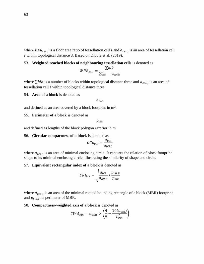
63

where 𝐹𝐴𝑅𝑐𝑒𝑙𝑙𝑖 is a floor area ratio of tessellation cell 𝑖 and 𝑎𝑐𝑒𝑙𝑙𝑖 is an area of tessellation cell

𝑖 within topological distance 3. Based on Dibble et al. (2019).

53. Weighted reached blocks of neighbouring tessellation cells is denoted as

𝑊𝑅𝐵𝑐𝑒𝑙𝑙 =∑𝑏𝑙𝑘

∑𝑛𝑖=1 𝑎𝑐𝑒𝑙𝑙𝑖

where ∑𝑏𝑙𝑘 is a number of blocks within topological distance three and 𝑎𝑐𝑒𝑙𝑙𝑖 is an area of

tessellation cell 𝑖 within topological distance three.

54. Area of a block is denoted as

𝑎𝑏𝑙𝑘

and defined as an area covered by a block footprint in m2.

55. Perimeter of a block is denoted as

𝑝𝑏𝑙𝑘

and defined as lengths of the block polygon exterior in m.

56. Circular compactness of a block is denoted as

𝐶𝐶𝑜𝑏𝑙𝑘 =𝑎𝑏𝑙𝑘𝑎𝑏𝑙𝑘𝐶

where 𝑎𝑏𝑙𝑘𝐶 is an area of minimal enclosing circle. It captures the relation of block footprint

shape to its minimal enclosing circle, illustrating the similarity of shape and circle.

57. Equivalent rectangular index of a block is denoted as

𝐸𝑅𝐼𝑏𝑙𝑘 = √𝑎𝑏𝑙𝑘𝑎𝑏𝑙𝑘𝐵

∗𝑝𝑏𝑙𝑘𝐵𝑝𝑏𝑙𝑘

where 𝑎𝑏𝑙𝑘𝐵 is an area of the minimal rotated bounding rectangle of a block (MBR) footprint

and 𝑝𝑏𝑙𝑘𝐵 its perimeter of MBR.

58. Compactness-weighted axis of a block is denoted as

𝐶𝑊𝐴𝑏𝑙𝑘 = 𝑑𝑏𝑙𝑘𝐶 × (4

𝜋−16(𝑎𝑏𝑙𝑘)

𝑝𝑏𝑙𝑘2 )

64

where 𝑑𝑏𝑙𝑘𝐶 is a diameter of the minimal circumscribed circle around the block polygon, 𝑎𝑏𝑙𝑘

is an area of a block and 𝑝𝑏𝑙𝑘 is a perimeter of a block. It is a proxy of permeability of an area

(Feliciotti, 2018).

59. Solar orientation of a block is denoted as

𝑂𝑟𝑖𝑏𝑙𝑘 = |𝑜𝑏𝑙𝑘𝐵 − 45|

where 𝑜𝑏𝑙𝑘𝐵 is an orientation of the longest axis of bounding rectangle in a range 0 - 45. It

captures the deviation of orientation from cardinal directions.

60. Weighted neighbours of a block is denoted as

𝑤𝑁𝑏𝑙𝑘 =∑𝑏𝑙𝑘𝑛𝑝𝑏𝑙𝑘

where ∑𝑏𝑙𝑘𝑛 is a number of block neighbours and 𝑝𝑏𝑙𝑘 is a perimeter of a block. It reflects

granularity of a mesh of blocks.

61. Weighted cells of a block is denoted as

𝑤𝐶𝑏𝑙𝑘 =∑𝑐𝑒𝑙𝑙

𝑎𝑏𝑙𝑘

where ∑𝑐𝑒𝑙𝑙 is a number of cells composing a block and 𝑎𝑏𝑙𝑘 is an area of a block. It captures

the granularity of each block.

62. Local meshedness of a street network is denoted as

𝑀𝑒𝑠𝑛𝑜𝑑𝑒 =𝑒 − 𝑣 + 1

2𝑣 − 5

where 𝑒 is a number of edges in a subgraph, and 𝑣 is the number of nodes in a subgraph

(Feliciotti, 2018). A subgraph is defined as a network within topological distance five around

a node.

63. Mean segment length of a street network is denoted as

𝑀𝑆𝐿𝑒𝑑𝑔 =1

𝑛∑

𝑛

𝑖=1

𝑙𝑒𝑑𝑔𝑖

where 𝑙𝑒𝑑𝑔𝑖 is a length of a street segment 𝑖 within a topological distance 3 around a segment.

64. Cul-de-sac length of a street network is denoted as

65

𝐶𝐷𝐿𝑛𝑜𝑑𝑒 =∑

𝑛

𝑖=1

𝑙𝑒𝑑𝑔𝑖 , 𝑖𝑓𝑒𝑑𝑔𝑖 𝑖𝑠𝑐𝑢𝑙 − 𝑑𝑒 − 𝑠𝑎𝑐

where 𝑙𝑒𝑑𝑔𝑖 is a length of a street segment 𝑖 within a topological distance 3 around a node.

65. Reached cells by street network segments is denoted as

𝑅𝐶𝑒𝑑𝑔 =∑

𝑛

𝑖=1

𝑐𝑒𝑙𝑙𝑠𝑒𝑑𝑔𝑖

where 𝑐𝑒𝑙𝑙𝑠𝑒𝑑𝑔𝑖 is number of tessellation cells on segment 𝑖 within topological distance 3. It

captures accessible granularity.

66. Node density of a street network is denoted as

𝐷𝑛𝑜𝑑𝑒 =∑𝑛𝑜𝑑𝑒

∑𝑛𝑖=1 𝑙𝑒𝑑𝑔𝑖

where ∑𝑛𝑜𝑑𝑒 is a number of nodes within a subgraph and 𝑙𝑒𝑑𝑔𝑖 is a length of a segment 𝑖

within a subgraph. A subgraph is defined as a network within topological distance five around

a node.

67. Reached cells by street network nodes is denoted as

𝑅𝐶𝑛𝑜𝑑𝑒𝑛𝑒𝑡 =∑

𝑛

𝑖=1

𝑐𝑒𝑙𝑙𝑠𝑛𝑜𝑑𝑒𝑖

where 𝑐𝑒𝑙𝑙𝑠𝑛𝑜𝑑𝑒𝑖 is number of tessellation cells on node 𝑖 within topological distance 3. It

captures accessible granularity.

68. Reached area by street network nodes is denoted as

𝑎𝑛𝑜𝑑𝑒𝑛𝑒𝑡 =∑

𝑛

𝑖=1

𝑎𝑛𝑜𝑑𝑒𝑖

where 𝑎𝑛𝑜𝑑𝑒𝑖 is an area covered by a street node 𝑖 within topological distance 3. It captures an

accessible area.

69. Proportion of cul-de-sacs within a street network is denoted as

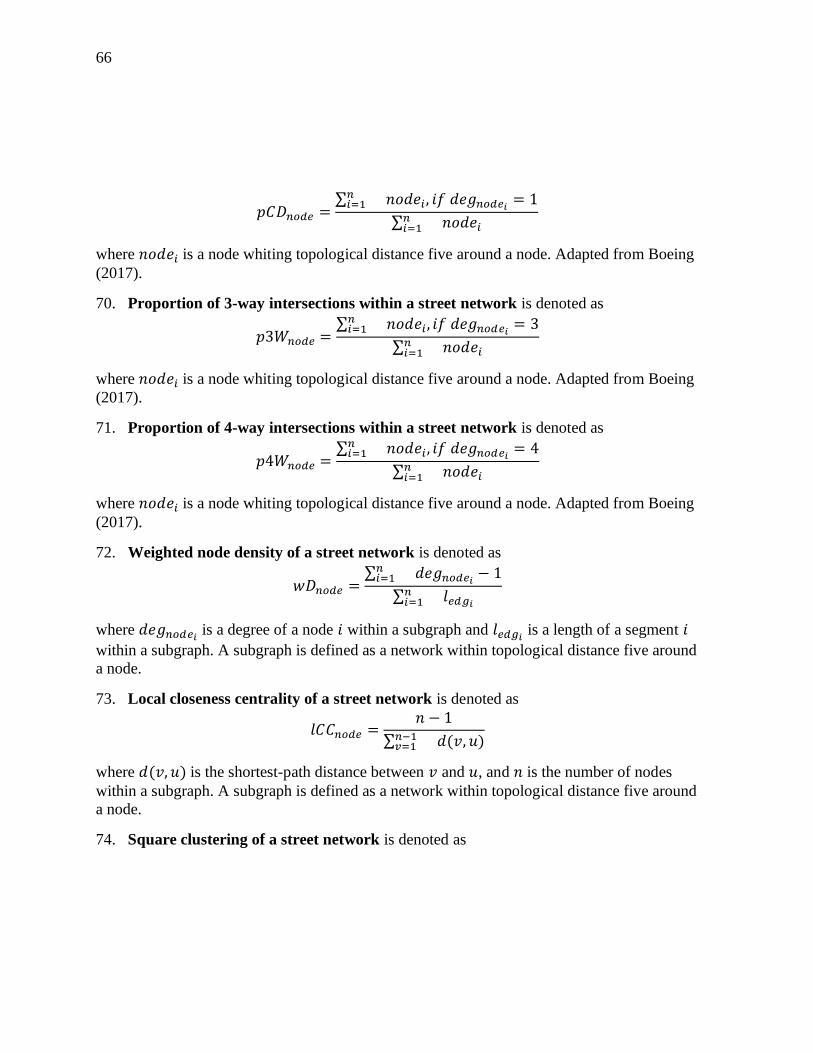
66

𝑝𝐶𝐷𝑛𝑜𝑑𝑒 =∑𝑛𝑖=1 𝑛𝑜𝑑𝑒𝑖 , 𝑖𝑓𝑑𝑒𝑔𝑛𝑜𝑑𝑒𝑖 = 1

∑𝑛𝑖=1 𝑛𝑜𝑑𝑒𝑖

where 𝑛𝑜𝑑𝑒𝑖 is a node whiting topological distance five around a node. Adapted from Boeing

(2017).

70. Proportion of 3-way intersections within a street network is denoted as

𝑝3𝑊𝑛𝑜𝑑𝑒 =∑𝑛𝑖=1 𝑛𝑜𝑑𝑒𝑖 , 𝑖𝑓𝑑𝑒𝑔𝑛𝑜𝑑𝑒𝑖 = 3

∑𝑛𝑖=1 𝑛𝑜𝑑𝑒𝑖

where 𝑛𝑜𝑑𝑒𝑖 is a node whiting topological distance five around a node. Adapted from Boeing

(2017).

71. Proportion of 4-way intersections within a street network is denoted as

𝑝4𝑊𝑛𝑜𝑑𝑒 =∑𝑛𝑖=1 𝑛𝑜𝑑𝑒𝑖 , 𝑖𝑓𝑑𝑒𝑔𝑛𝑜𝑑𝑒𝑖 = 4

∑𝑛𝑖=1 𝑛𝑜𝑑𝑒𝑖

where 𝑛𝑜𝑑𝑒𝑖 is a node whiting topological distance five around a node. Adapted from Boeing

(2017).

72. Weighted node density of a street network is denoted as

𝑤𝐷𝑛𝑜𝑑𝑒 =∑𝑛𝑖=1 𝑑𝑒𝑔𝑛𝑜𝑑𝑒𝑖 − 1

∑𝑛𝑖=1 𝑙𝑒𝑑𝑔𝑖

where 𝑑𝑒𝑔𝑛𝑜𝑑𝑒𝑖 is a degree of a node 𝑖 within a subgraph and 𝑙𝑒𝑑𝑔𝑖 is a length of a segment 𝑖

within a subgraph. A subgraph is defined as a network within topological distance five around

a node.

73. Local closeness centrality of a street network is denoted as

𝑙𝐶𝐶𝑛𝑜𝑑𝑒 =𝑛 − 1

∑𝑛−1𝑣=1 𝑑(𝑣, 𝑢)

where 𝑑(𝑣, 𝑢) is the shortest-path distance between 𝑣 and 𝑢, and 𝑛 is the number of nodes

within a subgraph. A subgraph is defined as a network within topological distance five around

a node.

74. Square clustering of a street network is denoted as

67

𝑠𝐶𝑙𝑛𝑜𝑑𝑒 =∑𝑘𝑣𝑢=1 ∑𝑘𝑣

𝑤=𝑢+1 𝑞𝑣(𝑢,𝑤)

∑𝑘𝑣𝑢=1

∑𝑘𝑣𝑤=𝑢+1

[𝑎𝑣(𝑢, 𝑤) + 𝑞𝑣(𝑢, 𝑤)]

where 𝑞𝑣(𝑢, 𝑤) are the number of common neighbours of 𝑢 and 𝑤 other than 𝑣 (ie squares),

and 𝑎𝑣(𝑢, 𝑤) = (𝑘𝑢 − (1 + 𝑞𝑣(𝑢,𝑤) + 𝜃𝑢𝑣))(𝑘𝑤 − (1 + 𝑞𝑣(𝑢, 𝑤) + 𝜃𝑢𝑤)), where 𝜃𝑢𝑤 = 1

if 𝑢 and 𝑤 are connected and 0 otherwise (Lind et al., 2005).

Table below contains each character and its classification to scale following <masked for

blind review> and key used in additional figures across supplementary materials.

index element grain extent id

area building S S sdbAre

height building S S sdbHei

volume building S S sdbVol

perimeter building S S sdbPer

courtyard area building S S sdbCoA

form factor building S S ssbFoF

volume to façade ratio building S S ssbVFR

circular compactness building S S ssbCCo

corners building S S ssbCor

squareness building S S ssbSqu

equivalent rectangular index building S S ssbERI

elongation building S S ssbElo

centroid - corner distance

deviation building S S ssbCCD

centroid - corner mean distance building S S ssbCCM

solar orientation building S S stbOri

street alignment building S S stbSAl

cell alignment building S S stbCeA

longest axis length tessellation cell S S sdcLAL

area tessellation cell S S sdcAre

circular compactness tessellation cell S S sscCCo

equivalent rectangular index tessellation cell S S sscERI

68

solar orientation tessellation cell S S stcOri

street alignment tessellation cell S S stcSAl

coverage area ratio tessellation cell S S sicCAR

floor area ratio tessellation cell S S sicFAR

length street segment S S sdsLen

width street profile S S sdsSPW

height street profile S S sdsSPH

height to width ratio street profile S S sdsSPR

openness street profile S S sdsSPO

width deviation street profile S S sdsSWD

height deviation street profile S S sdsSHD

linearity street segment S S sssLin

area covered street segment S S sdsAre

buildings per meter street segment S S sisBpM

area covered street node S S sddAre

shared walls ratio

adjacent

buildings S S mtbSWR

alignment

neighbouring

buildings S S mtbAli

mean distance

neighbouring

buildings S S mtbNDi

weighted neighbours tessellation cell S S mtcWNe

area covered

neighbouring

cells S S mdcAre

reached cells

neighbouring

segments S S misRea

reached area

neighbouring

segments S S mdsAre

degree street node S S mtdDeg

mean distance to neighbouring

nodes street node S S mtdMDi

reached cells

neighbouring

nodes S S midRea

reached area

neighbouring

nodes S S midAre

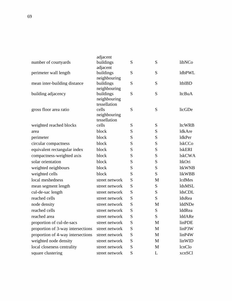
69

number of courtyards

adjacent

buildings S S libNCo

perimeter wall length

adjacent

buildings S S ldbPWL

mean inter-building distance

neighbouring

buildings S S ltbIBD

building adjacency

neighbouring

buildings S S ltcBuA

gross floor area ratio

neighbouring

tessellation

cells S S licGDe

weighted reached blocks

neighbouring

tessellation

cells S S ltcWRB

area block S S ldkAre

perimeter block S S ldkPer

circular compactness block S S lskCCo

equivalent rectangular index block S S lskERI

compactness-weighted axis block S S lskCWA

solar orientation block S S ltkOri

weighted neighbours block S S ltkWNB

weighted cells block S S likWBB

local meshedness street network S M lcdMes

mean segment length street network S S ldsMSL

cul-de-sac length street network S S ldsCDL

reached cells street network S S ldsRea

node density street network S M lddNDe

reached cells street network S S lddRea

reached area street network S S lddARe

proportion of cul-de-sacs street network S M linPDE

proportion of 3-way intersections street network S M linP3W

proportion of 4-way intersections street network S M linP4W

weighted node density street network S M linWID

local closeness centrality street network S M lcnClo

square clustering street network S L xcnSCl

70

Table S2: Additional classification of primary morphometric characters.

71

Supplementary Material 3: Bayesian Information Criterion

Figure S5: Bayesian Information Criterion score for the variable number of components in

Prague case study. Shaded area reflects .95 confidence interval.

72

Figure S6: Bayesian Information Criterion score for the variable number of components in

Amsterdam case study. Shaded area reflects .95 confidence interval, red line marks the first

significant minimum.

Supplementary material 4: Full extent of presented maps illustrating spatial distribution

of results of cluster analysis.

73

Figure S7: Spatial distribution of 10 detected clusters in Prague.

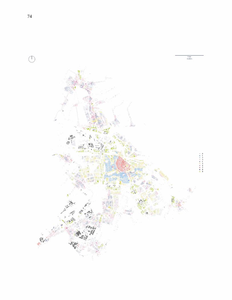
74

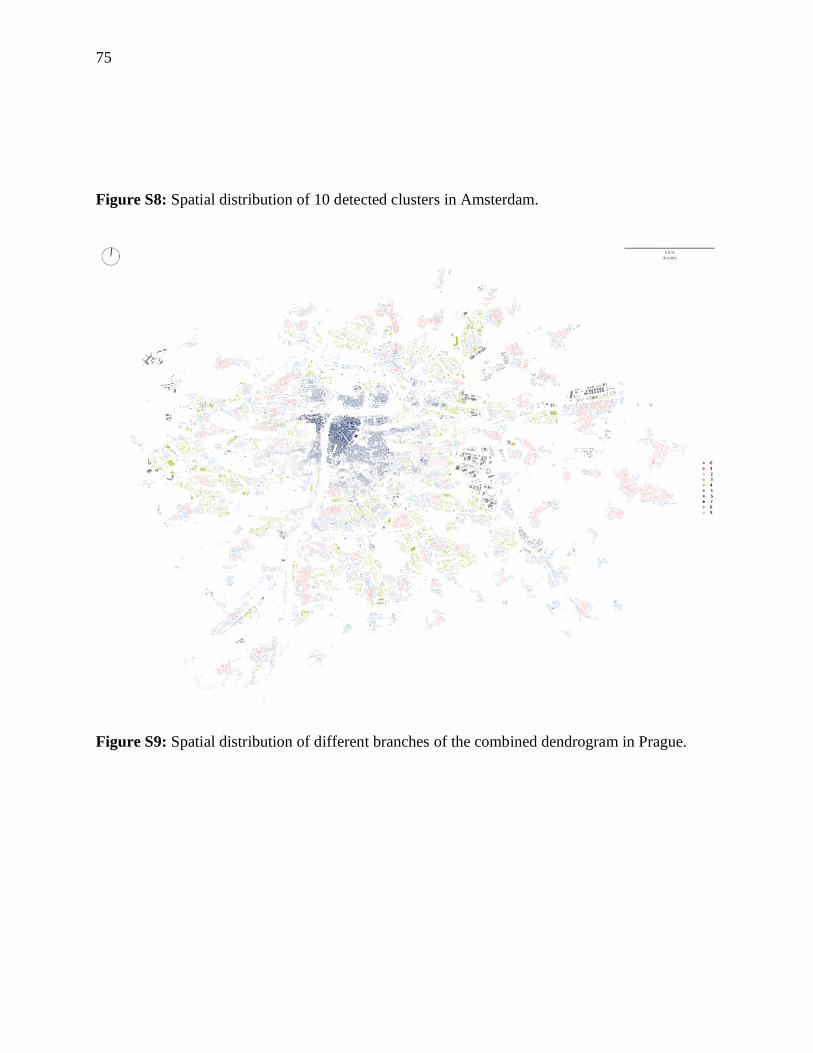
75

Figure S8: Spatial distribution of 10 detected clusters in Amsterdam.

Figure S9: Spatial distribution of different branches of the combined dendrogram in Prague.

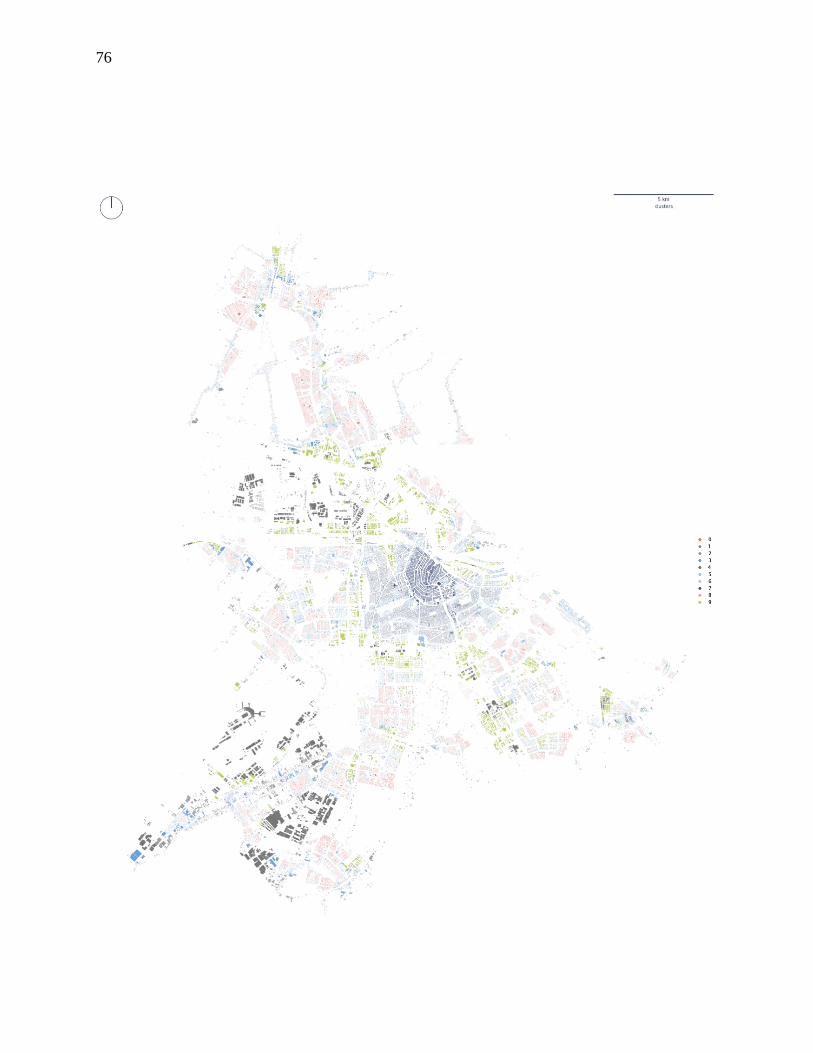
76

77

Figure S10: Spatial distribution of different branches of the combined dendrogram in

Amsterdam.

Supplementary Material 5: Contingency tables

,

cluster 1840 1880 1920 1950 1970 1990 2012

0 349 85 263 1219 1506 1442 565

1 1138 513 3588 17095 4499 1265 1453

2 1407 621 1655 4537 3108 2530 1357

3 1392 1719 2658 2895 678 223 213

4 145 54 156 888 1993 6414 532

5 3442 568 1487 7677 3975 2084 3459

6 1413 2778 4109 2005 150 4 8

7 3177 110 73 49 0 0 1

8 2834 981 2661 9645 4259 2629 829

9 69 63 151 3764 1147 1573 1244

Table S3: Contingency table showing the counts of features per historical origin within

individual clusters in Prague case study.

cluster

Multi-family

housing

Single-family

housing Villas

Industry

small

Industry

large other

0 112 617 3 322 1138 3497

1 437 27953 1164 3 0 33

2 3706 7238 203 972 789 2830

3 8472 577 136 93 26 626

4 9553 748 0 0 0 17

5 75 21590 147 50 22 1156

6 10070 231 153 0 0 34

7 2374 6 0 0 0 1057

8 4296 18110 1080 117 60 340

78

9 868 7015 79 0 0 120

Table S4: Contingency table showing the counts of features per predominant land use within

individual clusters in Prague case study.

cluster organic

perimeter

block village

garden

city modernism production services

0 0 17 377 213 39 3216 352

1 0 3 11384 16150 100 1 0

2 8 453 2937 2859 1394 2383 1085

3 192 6516 100 725 248 234 197

4 0 54 192 324 8782 17 49

5 0 0 13298 7824 40 33 61

6 604 8522 8 575 6 0 0

7 3281 49 0 0 0 3 78

8 0 263 6614 9900 2189 98 78

9 0 0 880 3176 1112 0 62

Table S5: Contingency table showing the counts of features per expert typology classes

within individual clusters in Prague case study.

cluster 1800 1850 1900 1930 1945 1960 1975 1985 1995 2005 2020

0 2 6 25 653 757 5541 11488 10448 10153 3362 3327

1 314 0 5201 17479 5118 325 60 395 743 241 110

2 65 42 360 1794 914 1409 1949 1258 1280 1597 1230

3 59 27 303 2133 1072 1244 2189 1512 1906 1990 1452

4 2 0 62 32 27 81 267 288 420 477 361

5 927 24 2000 5825 2824 6583 3236 2564 3854 3662 3393

6 111 45 713 5116 2366 4643 8811 4463 5696 4171 3089

7 7153 98 1531 1828 692 145 213 362 722 386 125

8 31 24 371 7976 6716 11113 5369 1948 7652 2948 3739

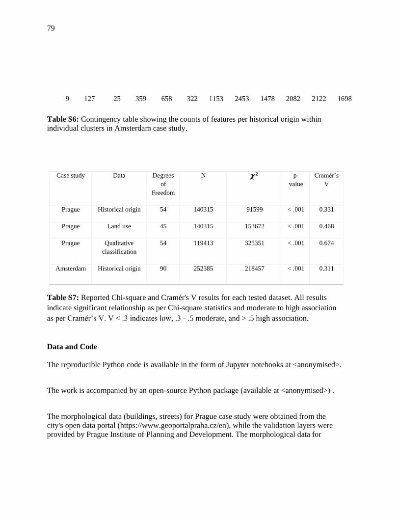
79

9 127 25 359 658 322 1153 2453 1478 2082 2122 1698

Table S6: Contingency table showing the counts of features per historical origin within

individual clusters in Amsterdam case study.

Case study Data Degrees

of

Freedom

N 𝝌𝟐 p-

value

Cramér’s

V

Prague Historical origin 54 140315 91599 < .001 0.331

Prague Land use 45 140315 153672 < .001 0.468

Prague Qualitative

classification

54 119413 325351 < .001 0.674

Amsterdam Historical origin 90 252385 218457 < .001 0.311

Table S7: Reported Chi-square and Cramér's V results for each tested dataset. All results

indicate significant relationship as per Chi-square statistics and moderate to high association

as per Cramér’s V. V < .3 indicates low, .3 - .5 moderate, and > .5 high association.

Data and Code

The reproducible Python code is available in the form of Jupyter notebooks at <anonymised>.

The work is accompanied by an open-source Python package (available at <anonymised>) .

The morphological data (buildings, streets) for Prague case study were obtained from the

city's open data portal (https://www.geoportalpraha.cz/en), while the validation layers were

provided by Prague Institute of Planning and Development. The morphological data for

80

Amsterdam are obtained from 3D BAG repository (Dukai, 2020) and Basisregistratie

Grootschalige Topografie, BGT (http://data.nlextract.nl/)

- Dukai, B. (2020) ‘3D Registration of Buildings and Addresses (BAG) / 3D

Basisregistratie Adressen en Gebouwen (BAG)’, 4TU.ResearchData. doi:

10.4121/uuid:f1f9759d-024a-492a-b821-07014dd6131c.