methodological documentation for the climate vulnerability …

METHODOLOGY NOTE

METHODOLOGICAL DOCUMENTATION FOR THE CLIMATE VULNERABILITY MONITOR 2nd Edition

This documentation will be subject to flagged updates in particular if i t is deemed useful following comments received and as proves feasible within the scope of the document.

This documentation is available online at: www.daraint.org/cvm2/method

SEPTEMBER 2012

V.1 APPROVED FOR DISTRIBUTION FOR EXTERNAL/PUBLIC DISTRIBUTION FROM 26 SEPTEMBER 2012

METHODOLOGY NOTE

2/121

CONTENTS

TABLE OF CONTENTS

1 I N T R O D U C T I O N 4 THE NEW MONITOR 4 INDEX ARCHITECTURE 7 CONFIDENCE/AGREEMENT/UNCERTAINTY 18 AFFECTED PEOPLE QUANTIFICATION 19

1 P A R T I : H A B I T A T C H A N G E 2 0 IMPACT AREA BASELINE DATA AND PROJECTIONS 21 BIODIVERSITY 21 DESERTIFICATION 23 HEATING & COOLING 24 LABOUR PRODUCTIVITY 26 PERMAFROST 28 SEA-LEVEL RISE 30 WATER 31

2 P A R T I : H E A L T H I M P A C T 3 4 IMPACT AREA BASELINE DATA AND PROJECTIONS 34 RESEARCH/DATA SOURCES: HEALTH IMPACT 35 ECONOMIC GROWTH ADJUSTEMENTS FOR 2030 36 HEALTH COSTS QUANTIFICATION 36 CALCULATION OF CLIMATE EFFECT: VECTOR-BORNE DISEASES, HUNGER AND DIARRHEAL INFECTIONS 37 CLIMATE IMPACT FACTORS 37 MENINGITIS 38 HEAT & COLD ILLNESSES (NON-INFLUENZA) 39 HEAT & COLD ILLNESSES (SKIN CANCER) 41 HEAT & COLD ILLNESSES (INFLUENZA) 42

3 P A R T I : I N D U S T R Y S T R E S S 4 4 IMPACT AREA BASELINE DATA AND PROJECTIONS 45 CLIMATE IMPACT FACTORS 45 AGRICULTURE 46 FISHERIES 47 FORESTRY 48 HYDRO ENERGY 50 TOURISM 52 TRANSPORT 55

4 P A R T I : E N V I R O N M E N T A L D I S A S T E R S 5 8 IMPACT AREA BASELINE DATA AND PROJECTIONS 59 RESEARCH/DATA SOURCES: ENVIRONMENTAL DISASTERS 59 CLIMATE IMPACT FACTORS 60 FLOODS & LANDSLIDES 60 STORMS 63

METHODOLOGY NOTE

3/121

WILDFIRES 65 DROUGHT 66 DROUGHT (SOIL SUBSIDENCE) 67

5 P A R T I I : B A S E I N D I C A T O R S – C A R B O N 7 0 POPULATION INDICATORS 70 ECONOMIC INDICATORS 70 EMISSION/PROJECTION SCENARIOS 70

6 P A R T I I : E N V I R O N M E N T A L D I S A S T E R S 7 2 OIL SANDS 72 OIL SPILLS 73

7 P A R T I I : H A B I T A T C H A N G E 7 6 BIODIVERSITY (OZONE) 76 BIODIVERSITY (ACID RAIN) 77 CORROSION 78 WATER 79

8 P A R T I I : H E A L T H I M P A C T 8 1 AIR POLLUTION 81 INDOOR SMOKE 83 OCCUPATIONAL HAZARDS 87

1 0 P A R T I I : I N D U S T R Y S T R E S S 9 3 AGRICULTURE (ACID RAIN) 93 AGRICULTURE (OZONE) 94 AGRICULTURE (GLOBAL DIMMING) 95 AGRICULTURE (CARBON FERTILIZATION) 96 MARINE FISHERIES (OCEAN ACIDIFICATION) 96 FORESTRY (OZONE) 98 FORESTRY (ACID RAIN) 99

9 C L I M A T E C H A N G E F I N A N C E 1 0 1 DATA SOURCES 101 OECD CREDITOR REPORTING SYSTEM 101 MULTI-LATERAL FUNDS 102

1 0 B I B L I O G R A P H Y 1 0 4

METHODOLOGY NOTE

4/121

1 INTRODUCTION

THE METHODOLOGY NOTE

This methodological documentation provides an explanation of how the quantitative architecture of the Climate Vulnerabil ity Monitor has been developed with detailed descriptions of each indicator relied upon and the aggregation and integration steps taken to create a common framework of analysis.

THE NEW MONITOR

GENERAL STRUCTURE OF NEW MONITOR

The Climate Vulnerabil ity Monitor (or “the Monitor”) in its 2nd edit ion is based on a quantitative framework comprised of two key parts as follows:

1 . Part I : A “Climate”*, meaning Climate Change, impact/vulnerabil ity assessment including 22 indicators across four Impact Areas (Environmental Disasters, Habitat Change, Health Impact, Industry Stress) measuring the posit ive and negative effects of climate change as they are experienced by 184 countries worldwide in socio-economic terms, in particular for the timeframes of 2010 and 2030. Part I/Climate relates to adaptation to climate change in that effective adaptation strategies and policies could target the minimization of the impacts/vulnerabil it ies assessed here.

2 . Part I I : A “Carbon”*, meaning carbon economy-related, impact/vulnerabil ity assessment including 12 indicators across the same four Impact Areas measuring the posit ive and negative effects of carbon-intensive energy reliance as experienced by countries worldwide in particular for 2010 and 2030. Part I I/Carbon relates to mitigation of climate change in that the impacts/vulnerabil it ies assessed here potentially represent co-benefits of different mitigation policies.

The Monitor has also been informed by two country studies, undertaken in Ghana and Vietnam, supported by hundreds of interviews in groups or individual settings, and national level workshops of key policy-makers. The Monitor additionally includes a review of international climate change financing, as well as analysis of allocations versus potential mitigation and adaptation co-benefits.

*See also the “Key Concepts and Definit ions” and “Methodology” sections of the 2nd Monitor report itself.

BASIC APPROACH

The Monitor aggregates together an internationally comparable and global picture of the current impact of climate change and the carbon economy as can be implied by current science and research. The chosen methodology that is the basis of the analysis of the Monitor’s second edit ion is described in detail here. Different methodologies would generate different results and reach different conclusions, just as the 2010 Monitor, with another methodology, differs from the latest version of the report in some of these respects.

METHODOLOGY NOTE

5/121

In effect, the Monitor seeks less to impose its own methodology, then to create and serve as a type of l inguistic framework for the latest leading scientif ic work and research on the impact of climate change/carbon-intensive practices to speak the same language. This methodology note is in many ways a log of what has not been done to the underlying research and data, exclusively drawn from recognized/authoritative external sources, very predominantly from peer-reviewed scientif ic l i terature. Where transformations have taken place efforts have been made to use simple adjustments, mainly in order to extrapolate effects from one or a l imited number of localit ies to other areas with similar hazard exposures and varying vulnerabil it ies – where research is more advanced, less interventions are made, and vice versa. Adjustments are also made in places to combine separate bodies of research within one indicator.

All of the key papers/research documents relied upon for each indicator are referenced in this methodology note. It is worth mention that a signif icant proportion of the research relied upon has only been made available since development of the first Monitor began in 2010, which underscores the pace at which this f ield of study is now evolving.

COUNTERFACTUAL ANALYSIS

When combing the full array of information the Monitor is each time attempting to measure the difference between a scenario with/without climate change (or the carbon economy), meaning, for instance, how many less (or more) l ives would be lost in a given year, and how much wealthier (or poorer) would economies be, i f there had not been climate change (or the carbon economy), which is “the counterfactual”. Independent research is piece-by-piece measuring some aspect of this difference - research the Monitor brings onto the same plane of interpretation. This analysis is notwithstanding cost-benefit/net benefit analysis of carbon-intensive versus low-carbon economic systems (i .e. the costs of mitigation), which is covered in the actual second edit ion Monitor report itself .

MONITOR OUTPUTS: IMPACTS AND VULNERABILITY LEVELS

The Monitor’s data outputs are given both as levels of vulnerabil ity and as estimates of the levels of absolute ( i .e. dollar gain) and/or relative (i .e. percentage loss of GDP) loss or gain – termed “impact” – implied by today’s (2010) or tomorrow’s (2030) situation, which is a scenario with cl imate change (N.B. information has also been compiled for the year 2000, however this data does not f igure in the f inal report) . With respect to vulnerabil ity, the level of impact is deemed indicative of the level of vulnerabil ity. Meaning, where impacts are more signif icant in relative terms (i .e. in relation to the size of the economy or population), vulnerabil ity is taken to be higher. The approach has been termed “outcome vulnerabil ity”, since it is the outcome of the vulnerabil ity – the degree/absence of harm incurred – that is the indicator of the level of vulnerabil ity present in the first place. Higher levels of impact are estimated, for instance, to have resulted from higher levels of vulnerabil ity, and vice versa, low levels of impact and vulnerabil ity go hand in hand. The Monitor expresses these vulnerabil ity levels in f ive categories, which are statistically determined using a (mean absolute) standard deviation approach, as follows:

• Acute (most vulnerable category)

• Severe

• High

• Moderate

• Low (least vulnerable category)

Countries with a level of vulnerabil ity of “Low” are most l ikely experiencing nil impact

METHODOLOGY NOTE

6/121

or benefits to some degree due to climate change. However, the purpose of the Monitor is not to pinpoint the level of benefits since the policy response is generally less relevant. Although, the Monitor does provide indications of the level of benefits in the outputted impact estimate data together with net results taking into account global gains and losses.

For the purpose of the Monitor and the indexes that the Monitor relies on, all impact estimates of gain or loss are measured only in mortality or share of GDP, so as to capture a comparable social or economic impact across wide-ranging countries. Equating all outputs to similar units means that diverse environmental phenomenon must be quantif ied in human terms or in economic terms, inside or outside the market, including for example, biodiversity, water resources and desertif ication – methodologies for translating these effects into economic data are drawn from relevant research or compiled and proposed where specif ic studies have not yet addressed the matter. GDP losses are 2010 USD PPP, although for 2030 losses these are additionally determined in relation to future expected economic development (but are not inflation adjusted for true 2030 dollars). Likewise, for mortality, the 2030 figures take into account projected population growth. All modeled data outputs in the Monitor in economic or other terms are rounded using a basic graded rounding protocol, which may be adapted for key sections.

THEMATIC AND INDEX-BASED FRAMEWORK

Each Part of the Monitor is constructed as a compilation of many different indicators that are each grouped under four themes per Part, termed Impact Areas, above all for ease of comprehension. The different impact areas are as follows:

Part I/”Climate” -

• Habitat Change – which measure the effects of climate change on aspects of human and ecological habitats and the economic gains and losses of these

• Health Impact – which measures the effects of climate change on human health and the social ( i .e. mortality) and economic gains and losses of this

• Industry Stress – which measures the effects of climate change on specif ic industry sectors of the economy, and the economic gains and losses of these

• Environmental Disasters – which measures the effects of climate change on one-off, punctual or geographically restricted extreme weather events, and the direct economic and social gains and losses of these

Part I I/”Carbon” -

• Environmental Disasters – which measures the effects of location or type specif ic environmental damage incidents and the economic gains/losses of these

• Habitat Change – which measures the effects of the carbon economy for aspects of human and ecological habitats and the economic gains/losses of these

• Health Impact – which measures the effects of the carbon economy on human health and the social and economic gains/losses of this

• Industry Stress – which measures the effects of the carbon economy on specif ic industry sectors of the economy, and the economic gains/losses of these

A series of indexes form the mathematical backbone of the statistical language that the Monitor uses in order to translate the implications of varied research in social or economic terms and aggregate or enumerate that information together. The indexes are presented in the Monitor is different ways: an overall index aggregating Part I and Part I I ; an aggregate index for Part I , and likewise for Part I I ; aggregate sub-indexes for the different impact areas (Habitat Change, etc.) which combine the indicators for each; and

METHODOLOGY NOTE

7/121

at the indicator level, single indexes for each group of effects form the foundation of the statistical architecture upon which the rest is built . Every category and indicator represents distinct climate impacts without overlap (or only statistically insignif icant/marginal overlap).

SPECIFIC APPROACH TO CLIMATE CHANGE

The Monitor takes a moderate precautionary approach to climate change and the effects of the carbon economy. As described in the relevant section below, mid to high range emission scenarios are chosen by default where possible. Likewise, means of estimates for impact/effects are taken where ranges are provided through research. This means a degree of under-counting as well as over-counting is possible versus what could be the reality of the situation. Despite its comprehensiveness, by no means are all of the effects of climate change/the carbon economy taken into account, mainly due to the l imitations of current research that any indicator in the Monitor must reflect.

The Monitor relies where feasible on empirical studies that observe as directly as possible the consequences of primary changes in the climate (such as temperature or rainfall change) on secondary phenomenon. Examples include the World Health Organization’s research into the implications of temperature and other climate-related variables as they react at the pathogen level of diseases, which has also been counter-verif ied in cases l ike diarrhea against information of disease prevalence versus climate parameters – i .e. hospital admittance rates during high temperatures episodes (McMicheal et al., 2004). However, in many cases, direct empirical evidence of effects on a global level is not possible. In these cases, the Monitor instead relies on a clear physical process and relationship for which there is both observational evidence and independent modeled agreement rather than on inconclusive and deficient instrumental records directly measuring the precise phenomenon of interest.

INDEX ARCHITECTURE

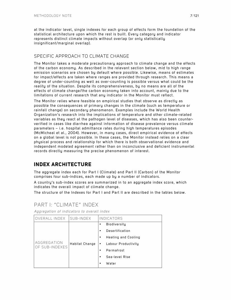
The aggregate index each for Part I (Climate) and Part I I (Carbon) of the Monitor comprises four sub-indices, each made up by a number of indicators.

A country’s sub-index scores are summarized in to an aggregate index score, which indicates the overall impact of climate change. The structure of the Indexes for Part I and Part I I are described in the tables below.

PART I: “CLIMATE” INDEX Aggregation of indicators to overall index

OVERALL INDEX SUB-INDEX INDICATORS

AGGREGATION OF SUB-INDEXES

Habitat Change

• Biodiversity

• Desert i f icat ion

• Heating and Cooling

• Labour Productivi ty

• Permafrost

• Sea-level Rise

• Water

METHODOLOGY NOTE

8/121

Health Impact

• Diarrheal Infect ions

• Heat & Cold I l lnesses

• Hunger

• Malaria & Vector-borne

• Meningit is

Industry Stress

• Agriculture

• Fisheries

• Forestry

• Hydro Energy

• Tourism

• Transport

Environmental Disasters

• Floods and landsl ides

• Storms

• Wildfires

• Drought

PART II: “CARBON” INDEX Aggregation of indicators to overall index

OVERALL INDEX SUB-INDEX INDICATORS

AGGREGATION OF SUB-INDEXES

Environmental Disasters

• Oil Sands

• Oil Spil ls

Habitat Change

• Biodiversity

• Corrosion

• Water

Health Impact

• Agriculture

• Air Pollut ion

• Indoor Smoke

• Occupational Hazards

Industry Stress

• Agriculture

• Fisheries

• Forestry

“CLIMATE/CARBON EFFECT”, “CLIMATE/CARBON IMPACT FACTOR”/”ATTRIBUTABLE FRACTION”, AND CLIMATE SCENARIO

The Monitor measures the impact of climate change or the carbon economy through socio-economic indicators based on a climate/carbon effect (CE).

METHODOLOGY NOTE

9/121

The Monitor assesses the CE in two ways as determined by the nature of the source information:

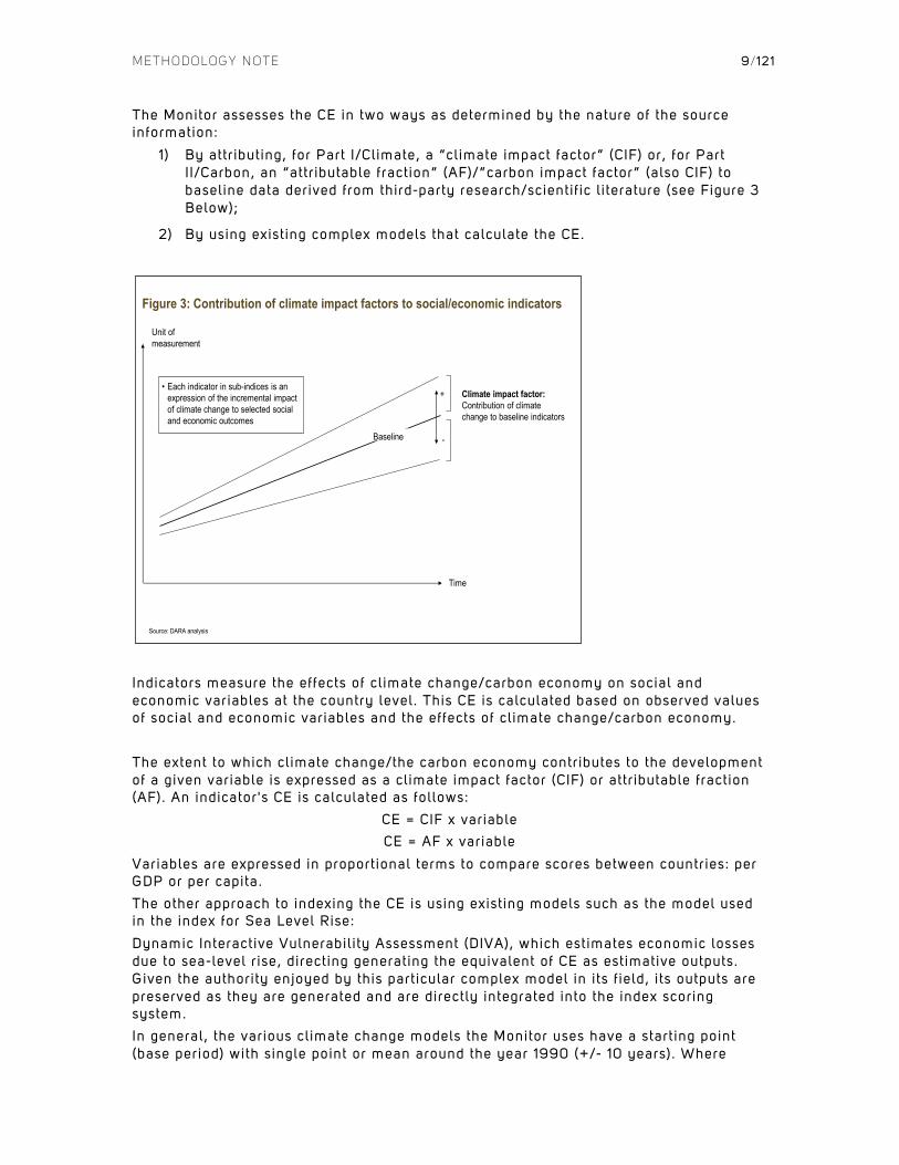
1) By attributing, for Part I/Climate, a “climate impact factor” (CIF) or, for Part I I/Carbon, an “attr ibutable fraction” (AF)/”carbon impact factor” (also CIF) to baseline data derived from third-party research/scientif ic l i terature (see Figure 3 Below);

2) By using existing complex models that calculate the CE.

Indicators measure the effects of climate change/carbon economy on social and economic variables at the country level. This CE is calculated based on observed values of social and economic variables and the effects of climate change/carbon economy.

The extent to which climate change/the carbon economy contributes to the development of a given variable is expressed as a climate impact factor (CIF) or attr ibutable fraction (AF). An indicator's CE is calculated as follows:

CE = CIF x variable CE = AF x variable

Variables are expressed in proportional terms to compare scores between countries: per GDP or per capita.

The other approach to indexing the CE is using existing models such as the model used in the index for Sea Level Rise:

Dynamic Interactive Vulnerabil ity Assessment (DIVA), which estimates economic losses due to sea-level r ise, directing generating the equivalent of CE as estimative outputs. Given the authority enjoyed by this particular complex model in its f ield, its outputs are preserved as they are generated and are directly integrated into the index scoring system.

In general, the various climate change models the Monitor uses have a start ing point (base period) with single point or mean around the year 1990 (+/- 10 years). Where

Figure 3: Contribution of climate impact factors to social/economic indicators

• Each indicator in sub-indices is an expression of the incremental impact of climate change to selected social and economic outcomes

Climate impact factor: Contribution of climate change to baseline indicators

+

-Baseline

Source: DARA analysis

Time

Unit of measurement

METHODOLOGY NOTE

10/121

applicable/possible, medium-range climate scenarios have been chosen for each indicator to calculate projections, except for in the sea-level r ise indicator, where a high-emission scenario. This is because recent research-based observations suggest that the high scenario is l ikely the most appropriate for sea-level r ise projections.

INDEX SCORING

Key purposes of an index in this context are deemed to include:

• Drawing attention to departures from average behaviour

• Enabling comparison between countries

• Monitoring of variable evolution over t ime

Constructing an index score based on a cross-section of univariate measures requires the choice of a transformation. In the context of monitoring climate-related impact, the transformation is expected to balance the following goals:

• Preservation of the shape of the original distribution

• Unit-free measure

• Similarity of scale across indices

• Robustness, in the sense that a few extreme observations must not hide changes in remaining observations

The dispersion measure used was chosen based on the following criteria:

• An affine transformation that preserves the shape of the original distribution

• Given a measure of dispersion expressed in units of the original distribution, if the measure is used as a normalizing factor, the resulting score is both unit-free and similar with respect to scale across indices

• Robust dispersion measures such as mean absolute deviation or median absolute deviation are preferable, since they are somewhat insensit ive to extreme observations. Mean absolute deviation (MAD) is the specif ic choice for dispersion measure, since it weighs in extreme observations to some degree, while median absolute deviation does not

The index scores are constructed so that a CE of 100 indicates a neutral climate/carbon effect (CIF=0; AF=0), while values above 100 indicate a negative climate/carbon effect, and values below 100 indicate a net gain from the impact of climate change/carbon economy.

On the sub-index level, the countries have received an index score between 50 and c.500. Data is standardized using the following formula:

Index score = ((SUM (CEt , i )/(10xMAD (SUM(CE2010))+1)x100

Where variable is an indicator representing each country (i ) at t=2000, 2010, 2030.

In sub-indices, variations in data are collapsed by dividing with 10*MAD. By adding 1 and finally multiplying by 100, a neutral or zero climate effect is expressed by 100 while values above 100 express a negative effect of climate change. The MAD is kept at a constant 2010 level to allow for variations over t ime.

The countries are categorized in bands made in steps of ½*MAD from 100. The construction of the scoring means that one MAD of the 2010 score equals 10, resulting in

METHODOLOGY NOTE

11/121

the category bands l isted below:

• Below 100 = Low (reflecting posit ive impact of climate change)

• 100-104.99 (1/2*MAD from 100) = Moderate

• 105-109.99 = High -

• 110-114.99 = High +

• 115-119.99 = Severe -

• 120-124.99 = Severe +

• 125-129.99 = Acute -

• 130 and above = Acute +

While comparatively Low is almost indefinite, ranging from an index score of 100 to 50. Moderate as a category has a narrower range than the other vulnerabil ity levels given, equivalent to one half level of that for High, Severe and Acute. This is because statistically for most indicators for 2010 a majority of countries is located within the Moderate band or just below it ( in Low), whereas in other half bands, there are generally far less countries. So in order not to have too many category names, the bandwidth is doubled with +or– given on occasion to indicate in which half category a country scored.

This construction method also enables an intuit ive comparison between index scores Past (2000), Now (2010) and in the Near Term (2030).

AGGREGATE/MULTI-DIMENSIONAL INDEX SCORING

The purpose of the aggregate index scoring – referred to a “Multi-Dimensional Vulnerabil ity” - is to:

• Reflect countries highly impacted in one or more of the of the sub-indices

• Ensure that outliers in one of the sub-indices are not reflected disproportionally in the overall index

To achieve this scoring each category band on each sub-index is given a number:

• Below 100 = 1

• 100-104.99 = 2

• 105-109.99 = 3

• 110-114.99 = 4

• 115-119.99 = 5

• 120-124.99 = 6

• 125-129.99 = 7

• 130-134.99 = 8

• 135 and above = 9

The countries’ average score on the sub-indices is calculated either for economic or mortality values only, but not combined, as follows e.g.:

Part I/I I Aggregate Index = Sub-Indices Mean (Health Impact + Environmental Disasters + Habitat Change + Industry Stress)

The countries are categorized by final score using the legend below (corresponding to half sub-index category scores):

METHODOLOGY NOTE

12/121

CATEGORIZATION By category scores

CATEGORY LOW HIGH

ACUTE >5

SEVERE >4 <=5

HIGH >3 <=4

MODERATE >2 <=3

LOW <=2

Other aggregates are provided for total deaths (mortality) and total costs (economic) for both Part I/Climate and Part I I/Carbon as well as overall/combined (climate+carbon).

GEOGRAPHIC CALCULATIONS

For many of the indexes, the data format, "ASCII grid", has been used to read and manipulate the data.

The figure above shows a schematic representation of the data structure. V(i, j ) represents the value of the variable in the cell ( i , j ) ; 1≤ i≤N is the longitude and 1≤ j≤M is the latitude. In general, the great majority of the data used has a resolution ranging from 0.5 to 5.0 degrees. It is therefore possible to say that for a typical resolution of 0.5° X 0.5° the matrix has a size of (720,360). In some cases, several matrices were combined in order to obtain the value of a particular variable in a specif ic f ield. When the resolution of the data sources was different, a simple standardization process was applied, which downscaled all the grids to the one with the highest resolution

METHODOLOGY NOTE

13/121

keeping constant the value of the variable in the previous domain. A similar process was used if the grid f i les had different mapping origins. To obtain the values of a variable in a specif ic country, a grid map with a resolution of 0.5° was used, and every cell has a particular value associated with the country included. Therefore:

Value(country_k) = A(V(i, j ) ) where Map(i, j )=k where A is a generic operator and Map the countries data matrix. I t is clear that this technique has different advantages that avoid projection problems and simplify the entire algorithm. However, the overall resolution changes in function of the latitude in the following way:

S=( π/180) x R^2 x |sin(lat1)-sin(lat2)| x | lon1-lon2| where S is the surface between two defined latitudes and longitudes (lat1,lat2 and lon1,lon2) on a sphere. The major challenge associated with this approach is to model realistically countries with a size smaller than the grid cell that at the equator measure approximately 3000 Km^2. To avoid possible overestimations, a regional mean has been calculated and applied to the country's actual surface.

COUNTRIES INCLUDED AND SPATIAL SCALE

The index is calculated for 184 countries given the global focus and due to the upper l imits of data availabil ity for small numbers of countries, particularly Small Island Developing States (SIDSs) that have not met the minimum requirements for data. Since its main objective is to enable comparisons between nations and sub-regions, it measures vulnerabil ity at the national level. Assessment of vulnerabil ity at the sub-national and local level is beyond the scope of this report aside from conclusions of the field research and national workshops undertaken as a part of the Country Studies for the Monitor.

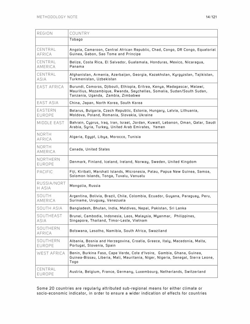
Countries are divided into 21 regions for presentation purposes. These sub-regions provide the basis for extrapolations of data when countries – habitually small island developing states with populations below 250,000 people – do not have adequate information to generate endogenous results. For instance, if no results are able to be obtained for Marshall Islands, Marshall Islands is attr ibuted a GDP or Population scaled regional mean from all Pacif ic countries.

REGIONS & COUNTRIES List of countries by Monitor sub-region

REGION COUNTRY

AUSTRALASIA Austral ia, New Zealand

CARIBBEAN Antigua and Barbuda, Bahamas, Barbados, Cuba, Dominica, Dominican Republic, Grenada, Hait i , Jamaica, Saint Lucia, Saint Vincent, Tr inidad and

METHODOLOGY NOTE

14/121

REGION COUNTRY

Tobago

CENTRAL AFRICA

Angola, Cameroon, Central Afr ican Republic, Chad, Congo, DR Congo, Equatorial Guinea, Gabon, Sao Tome and Principe

CENTRAL AMERICA

Belize, Costa Rica, El Salvador, Guatemala, Honduras, Mexico, Nicaragua, Panama

CENTRAL ASIA

Afghanistan, Armenia, Azerbai jan, Georgia, Kazakhstan, Kyrgyzstan, Taj ik istan, Turkmenistan, Uzbekistan

EAST AFRICA Burundi, Comoros, Dj ibouti , Ethiopia, Eri trea, Kenya, Madagascar, Malawi, Maurit ius, Mozambique, Rwanda, Seychelles, Somalia, Sudan/South Sudan, Tanzania, Uganda, Zambia, Zimbabwe

EAST ASIA China, Japan, North Korea, South Korea

EASTERN EUROPE

Belarus, Bulgaria, Czech Republic, Estonia, Hungary, Latvia, Lithuania, Moldova, Poland, Romania, Slovakia, Ukraine

MIDDLE EAST Bahrain, Cyprus, I raq, I ran, Israel, Jordan, Kuwait , Lebanon, Oman, Qatar, Saudi Arabia, Syria, Turkey, United Arab Emirates, Yemen

NORTH AFRICA

Algeria, Egypt, Libya, Morocco, Tunisia

NORTH AMERICA

Canada, United States

NORTHERN EUROPE

Denmark, Finland, Iceland, I reland, Norway, Sweden, United Kingdom

PACIFIC Fij i , Kir ibati , Marshall Is lands, Micronesia, Palau, Papua New Guinea, Samoa, Solomon Islands, Tonga, Tuvalu, Vanuatu

RUSSIA/NORTH ASIA

Mongolia, Russia

SOUTH AMERICA

Argentina, Bolivia, Brazil , Chile, Colombia, Ecuador, Guyana, Paraguay, Peru, Suriname, Uruguay, Venezuela

SOUTH ASIA Bangladesh, Bhutan, India, Maldives, Nepal, Pakistan, Sri Lanka

SOUTHEAST ASIA

Brunei, Cambodia, Indonesia, Laos, Malaysia, Myanmar, Phil ippines, Singapore, Thailand, Timor-Leste, Vietnam

SOUTHERN AFRICA

Botswana, Lesotho, Namibia, South Afr ica, Swaziland

SOUTHERN EUROPE

Albania, Bosnia and Herzegovina, Croatia, Greece, I taly, Macedonia, Malta, Portugal, Slovenia, Spain

WEST AFRICA Benin, Burkina Faso, Cape Verde, Cote d' Ivoire, Gambia, Ghana, Guinea, Guinea-Bissau, Liberia, Mali , Mauritania, Niger, Nigeria, Senegal, Sierra Leone, Togo

CENTRAL EUROPE

Austr ia, Belgium, France, Germany, Luxembourg, Netherlands, Switzerland

Some 20 countries are regularly attr ibuted sub-regional means for either climate or socio-economic indicator, in order to ensure a wider indication of effects for countries

METHODOLOGY NOTE

15/121

that would otherwise not be able to manifest results. These countries are as follows:

Cuba Dominica

Dominican Republic Fij i

Grenada Haiti

Jamaica Kiribati

Marshall Islands Micronesia

Palau Papua New Guinea

Saint Lucia Saint Vincent

Samoa Solomon Islands

Tonga Trinidad and Tobago

Tuvalu Vanuatu

The information in the report is presented throughout for four key country groups, called emission groups, based on the United Nations Framework Convention on Climate Change (UNFCCC) and on the emission levels of countries. These four groups are as follows in the table below. “Developed” countries are the Annex II state parties to the UNFCCC. “Other Industrialized” countries are the remainder of the Annex I state parties to the UNFCCC. “Developing countries”, all non-Annex I/I I countries, are divided into two categories based on their mean per capita emissions in 2005 for all Kyoto Protocol greenhouse gas emissions including for land use change and forestry (LULUCF). The threshold is set at 4 tons per capita of CO2 equivalent, which broadly implies that countries below this threshold may not need to take (any/extensive) mitigation measures in order to achieve an equitable average of per capita emissions level by 2020 congruent with achieving the international temperature rise goal of 2.0 degrees Celsius.

EMISSION GROUPS List of countries by main Monitor emission groups

GROUP COUNTRY

DEVELOPED (ANNEX II)

Austral ia, Austr ia, Belgium, Canada, Denmark, Finland, France, Germany,

Greece, Iceland, Ireland, I taly, Japan, Luxembourg, Netherlands, New Zealand,

Norway, Portugal, Spain, Sweden, Switzerland, United Kingdom, United States

OTHER INDUSTRIALIZED (ANNEX I OUTSIDE OF ANNEX II)

Belarus, Bulgaria, Croatia, Czech Republic, Estonia, Hungary, Latvia, Lithuania,

Malta, Poland, Romania, Russia, Slovakia, Slovenia, Turkey, Ukraine

DEVELOPING COUNTRY HIGH EMITTERS (NON-ANNEX I ABOVE 4 TONS CO2E 2005)

Algeria, Antigua and Barbuda, Argentina, Azerbai jan, Bahamas, Bahrain, Belize,

Bolivia, Bosnia and Herzegovina, Botswana, Brazil , Brunei, Bulgaria, Cambodia,

Central Afr ican Republic, Chile, China, Congo, Cote d’ Ivoire, Cyprus, DR Congo,

Equatorial Guinea, Gabon, Grenada, Guatemala, Guinea, Guyana, Indonesia,

I ran, I raq, Israel, Kazakhstan, Kuwait , Laos, Libya, Macedonia, Malaysia,

Mexico, Mongolia, Myanmar, Namibia, North Korea, Oman, Papua New Guinea,

Paraguay, Qatar, Saudi Arabia, Seychelles, Singapore, Solomon Islands, South

Afr ica, South Korea, Suriname, Thailand, Trinidad and Tobago, Turkmenistan,

United Arab Emirates, Uruguay, Uzbekistan, Venezuela, Zambia

METHODOLOGY NOTE

16 /121

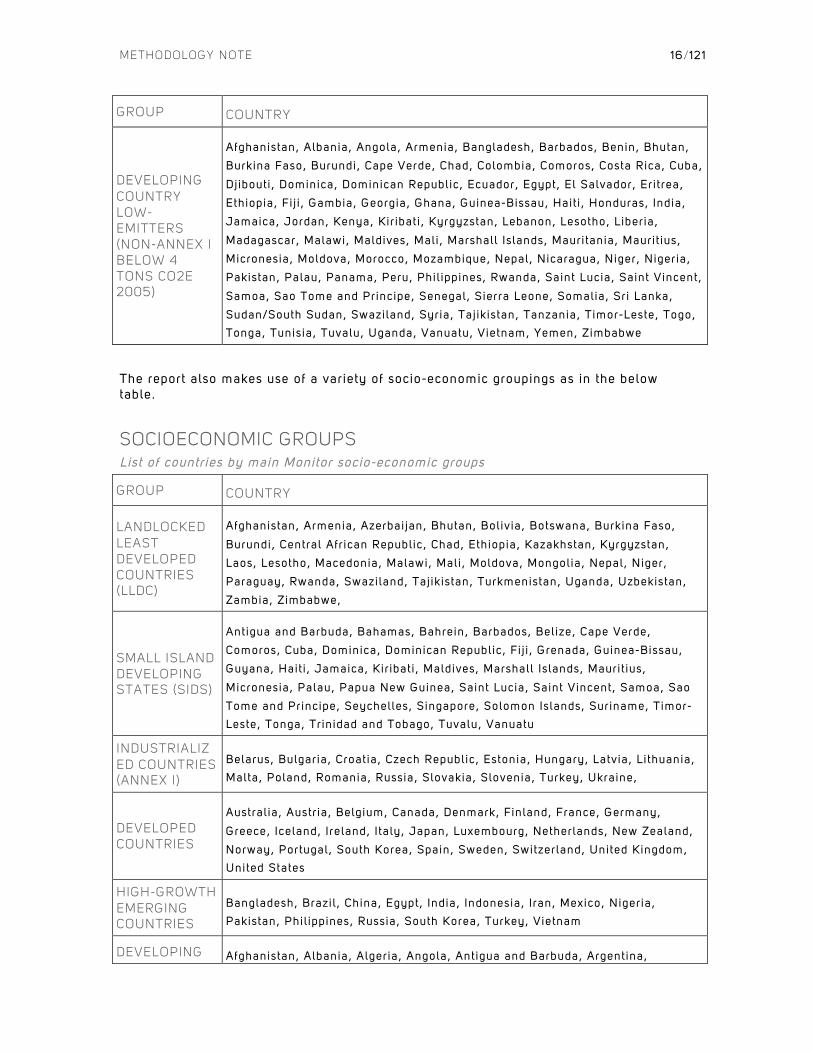
GROUP COUNTRY

DEVELOPING COUNTRY LOW-EMITTERS (NON-ANNEX I BELOW 4 TONS CO2E 2005)

Afghanistan, Albania, Angola, Armenia, Bangladesh, Barbados, Benin, Bhutan,

Burkina Faso, Burundi, Cape Verde, Chad, Colombia, Comoros, Costa Rica, Cuba,

Dj ibouti , Dominica, Dominican Republic, Ecuador, Egypt, El Salvador, Eri trea,

Ethiopia, Fi j i , Gambia, Georgia, Ghana, Guinea-Bissau, Hait i , Honduras, India,

Jamaica, Jordan, Kenya, Kir ibat i , Kyrgyzstan, Lebanon, Lesotho, Liberia,

Madagascar, Malawi, Maldives, Mali , Marshall Is lands, Mauritania, Maurit ius,

Micronesia, Moldova, Morocco, Mozambique, Nepal, Nicaragua, Niger, Nigeria,

Pakistan, Palau, Panama, Peru, Phil ippines, Rwanda, Saint Lucia, Saint Vincent,

Samoa, Sao Tome and Principe, Senegal, Sierra Leone, Somalia, Sri Lanka,

Sudan/South Sudan, Swaziland, Syria, Taj ikistan, Tanzania, Timor-Leste, Togo,

Tonga, Tunisia, Tuvalu, Uganda, Vanuatu, Vietnam, Yemen, Zimbabwe

The report also makes use of a variety of socio-economic groupings as in the below table.

SOCIOECONOMIC GROUPS List of countries by main Monitor socio-economic groups

GROUP COUNTRY

LANDLOCKED LEAST DEVELOPED COUNTRIES (LLDC)

Afghanistan, Armenia, Azerbai jan, Bhutan, Bolivia, Botswana, Burkina Faso,

Burundi, Central Afr ican Republic, Chad, Ethiopia, Kazakhstan, Kyrgyzstan,

Laos, Lesotho, Macedonia, Malawi, Mali , Moldova, Mongolia, Nepal, Niger,

Paraguay, Rwanda, Swaziland, Taj ik istan, Turkmenistan, Uganda, Uzbekistan,

Zambia, Zimbabwe,

SMALL ISLAND DEVELOPING STATES (SIDS)

Antigua and Barbuda, Bahamas, Bahrein, Barbados, Belize, Cape Verde,

Comoros, Cuba, Dominica, Dominican Republic, Fi j i , Grenada, Guinea-Bissau,

Guyana, Hait i , Jamaica, Kir ibat i , Maldives, Marshall Is lands, Maurit ius,

Micronesia, Palau, Papua New Guinea, Saint Lucia, Saint Vincent, Samoa, Sao

Tome and Principe, Seychelles, Singapore, Solomon Islands, Suriname, Timor-

Leste, Tonga, Trinidad and Tobago, Tuvalu, Vanuatu

INDUSTRIALIZED COUNTRIES (ANNEX I)

Belarus, Bulgaria, Croatia, Czech Republic, Estonia, Hungary, Latvia, Lithuania,

Malta, Poland, Romania, Russia, Slovakia, Slovenia, Turkey, Ukraine,

DEVELOPED COUNTRIES

Austral ia, Austr ia, Belgium, Canada, Denmark, Finland, France, Germany,

Greece, Iceland, Ireland, I taly, Japan, Luxembourg, Netherlands, New Zealand,

Norway, Portugal, South Korea, Spain, Sweden, Switzerland, United Kingdom,

United States

HIGH-GROWTH EMERGING COUNTRIES

Bangladesh, Brazil , China, Egypt, India, Indonesia, I ran, Mexico, Nigeria,

Pakistan, Phil ippines, Russia, South Korea, Turkey, Vietnam

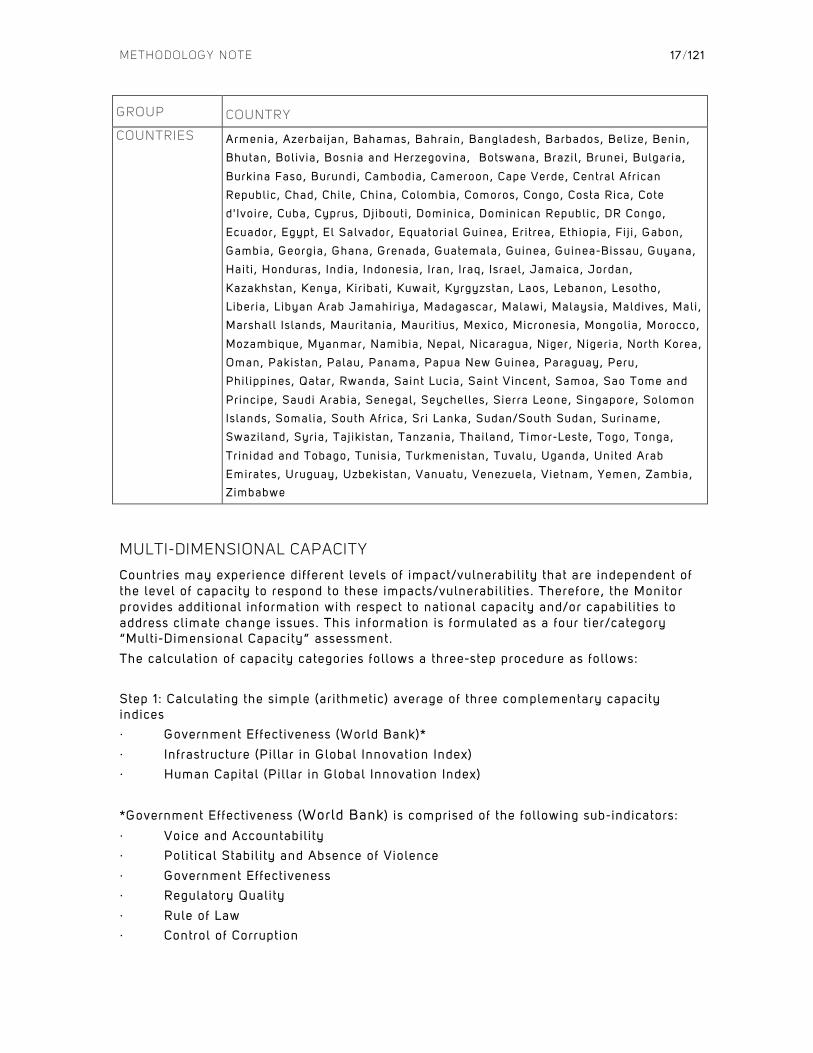
DEVELOPING Afghanistan, Albania, Algeria, Angola, Antigua and Barbuda, Argentina,

METHODOLOGY NOTE

17/121

GROUP COUNTRY

COUNTRIES Armenia, Azerbai jan, Bahamas, Bahrain, Bangladesh, Barbados, Belize, Benin,

Bhutan, Bolivia, Bosnia and Herzegovina, Botswana, Brazil , Brunei, Bulgaria,

Burkina Faso, Burundi, Cambodia, Cameroon, Cape Verde, Central Afr ican

Republic, Chad, Chile, China, Colombia, Comoros, Congo, Costa Rica, Cote

d' Ivoire, Cuba, Cyprus, Dj ibouti , Dominica, Dominican Republic, DR Congo,

Ecuador, Egypt, El Salvador, Equatorial Guinea, Eri trea, Ethiopia, Fi j i , Gabon,

Gambia, Georgia, Ghana, Grenada, Guatemala, Guinea, Guinea-Bissau, Guyana,

Hait i , Honduras, India, Indonesia, I ran, I raq, Israel, Jamaica, Jordan,

Kazakhstan, Kenya, Kir ibati , Kuwait , Kyrgyzstan, Laos, Lebanon, Lesotho,

Liberia, Libyan Arab Jamahir iya, Madagascar, Malawi, Malaysia, Maldives, Mali ,

Marshall Is lands, Mauritania, Maurit ius, Mexico, Micronesia, Mongolia, Morocco,

Mozambique, Myanmar, Namibia, Nepal, Nicaragua, Niger, Nigeria, North Korea,

Oman, Pakistan, Palau, Panama, Papua New Guinea, Paraguay, Peru,

Phil ippines, Qatar, Rwanda, Saint Lucia, Saint Vincent, Samoa, Sao Tome and

Principe, Saudi Arabia, Senegal, Seychelles, Sierra Leone, Singapore, Solomon

Islands, Somalia, South Afr ica, Sri Lanka, Sudan/South Sudan, Suriname,

Swaziland, Syria, Taj ikistan, Tanzania, Thailand, Timor-Leste, Togo, Tonga,

Trinidad and Tobago, Tunisia, Turkmenistan, Tuvalu, Uganda, United Arab

Emirates, Uruguay, Uzbekistan, Vanuatu, Venezuela, Vietnam, Yemen, Zambia,

Zimbabwe

MULTI-DIMENSIONAL CAPACITY

Countries may experience different levels of impact/vulnerabil ity that are independent of the level of capacity to respond to these impacts/vulnerabil it ies. Therefore, the Monitor provides additional information with respect to national capacity and/or capabil it ies to address climate change issues. This information is formulated as a four t ier/category “Multi-Dimensional Capacity” assessment.

The calculation of capacity categories follows a three-step procedure as follows:

Step 1: Calculating the simple (arithmetic) average of three complementary capacity indices · Government Effectiveness (World Bank)*

· Infrastructure (Pillar in Global Innovation Index) · Human Capital (Pillar in Global Innovation Index)

*Government Effectiveness (World Bank) is comprised of the following sub-indicators:

· Voice and Accountabil ity · Polit ical Stabil ity and Absence of Violence

· Government Effectiveness · Regulatory Quality

· Rule of Law · Control of Corruption

METHODOLOGY NOTE

18/121

The three indices all range from 0-100, with capacity increasing in the index score; i .e. the higher the score the higher the capacity.

Step 2: Weighing the average by

· Population (UN population) · National income (GNI per capita, UN DESA)

The weights run through 0.50, 0.75, 1.00 and 1.25, where 0.50 represents the lowest quartile and 1.25 represents the highest quartile.

The rationale is that countries with larger populations and national income have a greater capacity to mobilize a response to climatic challenges.

Step 3: Categorizing by quartiles

The numerical capacity index is sorted and capacity categories are assigned according to quartiles.

· Extensive capacity (3rd to 4th) · Intermediary capacity (2nd to 3rd)

· Restricted capacity (1st to 2nd) · Highly restricted capacity ( - 1st)

CONFIDENCE/AGREEMENT/UNCERTAINTY

The Monitor presents a range of information relating to the confidence of different indicators, the agreement of different research/models or not as relates to these indicators, and levels of uncertainty associated with each.

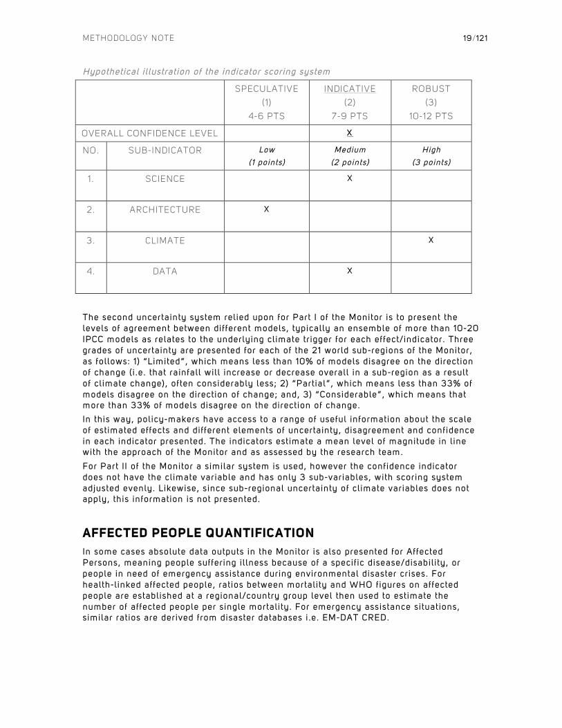
For Part I of the Monitor, two different indication sets are provided. First is a confidence indicator, which has three overall scores, from highest confidence to lowest confidence, termed as follows: 1) “Robust”; 2) “Indicative”; and, 3) “Speculative”. One of three overall scores is attr ibuted on the basis of the research teams’ assessment of four different criteria, which itself is a three point scale from low (1) through to high (3) confidence – each assessed in relative terms in the context of the overall f ield of climate change research and in relation to the various indicators of the Monitor. These are: f irst, “Science”, which refers in particular to recent IPCC confidence in that primary and secondary effects analyzed are clear manifestations of climate change or not; second, “Architecture”, which refers to the sophistication and robustness of the indicator as grounded in underlying studies – as an example, sophisticated multiple country study global models from peer reviewed literature score high; third, “Climate”, refers to the degree of agreement or not between different interpretations of effects, particularly magnitude – climate science may agree an effect is related to climate change but models may predict scales of increases or decrease for different regions with a high degree of discord, which is captured here; fourth, “Data”, refers to the relative quality of baseline socio-economic data relied upon, in particular, i ts international span and comparabil ity, as well as the level of precision it is understood to carry. The below table provides an example of how the Confidence indicator scoring system operates.

CONFIDENCE INDICATOR EXAMPLE

METHODOLOGY NOTE

19/121

Hypothetical i l lustration of the indicator scoring system

SPECULATIVE

(1)

4-6 PTS

INDICATIVE

(2)

7-9 PTS

ROBUST

(3)

10-12 PTS

OVERALL CONFIDENCE LEVEL X

NO. SUB-INDICATOR Low (1 points)

Medium (2 points)

High (3 points)

1. SCIENCE

X

2. ARCHITECTURE

X

3. CLIMATE

X

4. DATA

X

The second uncertainty system relied upon for Part I of the Monitor is to present the levels of agreement between different models, typically an ensemble of more than 10-20 IPCC models as relates to the underlying climate tr igger for each effect/indicator. Three grades of uncertainty are presented for each of the 21 world sub-regions of the Monitor, as follows: 1) “Limited”, which means less than 10% of models disagree on the direction of change (i .e. that rainfall will increase or decrease overall in a sub-region as a result of climate change), often considerably less; 2) “Partial”, which means less than 33% of models disagree on the direction of change; and, 3) “Considerable”, which means that more than 33% of models disagree on the direction of change.

In this way, policy-makers have access to a range of useful information about the scale of estimated effects and different elements of uncertainty, disagreement and confidence in each indicator presented. The indicators estimate a mean level of magnitude in l ine with the approach of the Monitor and as assessed by the research team.

For Part I I of the Monitor a similar system is used, however the confidence indicator does not have the climate variable and has only 3 sub-variables, with scoring system adjusted evenly. Likewise, since sub-regional uncertainty of climate variables does not apply, this information is not presented.

AFFECTED PEOPLE QUANTIFICATION

In some cases absolute data outputs in the Monitor is also presented for Affected Persons, meaning people suffering il lness because of a specif ic disease/disabil ity, or people in need of emergency assistance during environmental disaster crises. For health-linked affected people, ratios between mortality and WHO figures on affected people are established at a regional/country group level then used to estimate the number of affected people per single mortality. For emergency assistance situations, similar ratios are derived from disaster databases i .e. EM-DAT CRED.

METHODOLOGY NOTE

20/121

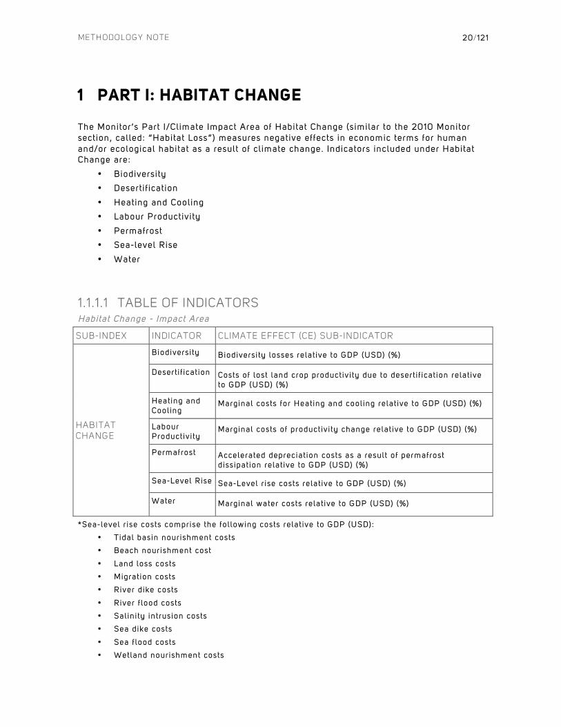
1 PART I: HABITAT CHANGE

The Monitor’s Part I/Climate Impact Area of Habitat Change (similar to the 2010 Monitor section, called: “Habitat Loss”) measures negative effects in economic terms for human and/or ecological habitat as a result of climate change. Indicators included under Habitat Change are:

• Biodiversity

• Desertif ication

• Heating and Cooling

• Labour Productivity

• Permafrost

• Sea-level Rise

• Water

1.1.1.1 TABLE OF INDICATORS Habitat Change - Impact Area

SUB-INDEX INDICATOR CLIMATE EFFECT (CE) SUB-INDICATOR

HABITAT CHANGE

Biodiversity Biodiversity losses relat ive to GDP (USD) (%)

Desert i f icat ion Costs of lost land crop productivi ty due to desert i f icat ion relat ive to GDP (USD) (%)

Heating and Cooling

Marginal costs for Heating and cooling relat ive to GDP (USD) (%)

Labour Productivi ty

Marginal costs of productivi ty change relat ive to GDP (USD) (%)

Permafrost Accelerated depreciat ion costs as a result of permafrost dissipation relat ive to GDP (USD) (%)

Sea-Level Rise Sea-Level r ise costs relat ive to GDP (USD) (%)

Water Marginal water costs relat ive to GDP (USD) (%)

*Sea-level r ise costs comprise the fol lowing costs relat ive to GDP (USD):

• Tidal basin nourishment costs

• Beach nourishment cost

• Land loss costs

• Migration costs

• River dike costs

• River f lood costs

• Salinity intrusion costs

• Sea dike costs

• Sea f lood costs

• Wetland nourishment costs

METHODOLOGY NOTE

21/121

N.B. the DIVA model est imates protect ion costs, such as Sea dike costs, when these costs are lower than the value of land that would otherwise be lost i f not protected.

The total excess damage costs due to climate change for a country is the sum of the CE for the indicators comprising the sub-index Habitat degradation:

• SUM (CE2010 ,gdp) = CE_SLR2010 , + CE_Desertif ication2010 + CE_Water2010 + CE_Permafrost2010 + CE_Biodiversity2010

The sub-index score is calculated by using the index calculation formula below:

• Index score 2010 = ((SUM (CE2010 ,gdp)/(10xMAD(SUM(CE2010 ,gdp))+1)x100

IMPACT AREA BASELINE DATA AND PROJECTIONS

SOCIOECONOMIC BASELINE Habitat Change

DEFINITION RESOLUTION SOURCE

GDP 2010 in 2010 USD (by country)

Country level, 184 countr ies IMF, World Economic Outlook Database, September 2011

SOCIOECONOMIC PROJECTION Habitat Change

DEFINITION RESOLUTION SCENARIOS SOURCE

Relative change in real GDP 2010 to 2030

Country level, 184 countr ies

SRES A1B CIESIN

BIODIVERSITY

RESEARCH/DATA SOURCES: BIODIVERSITY

CLIMATE IMPACT FACTOR Biodiversity

DEFINITION Addit ional losses in 2050 compared to 2000

SOURCE(S) The value of the world’s ecosystem services and natural capital, Costanza et al. , 1997.

Extinction risk from climate change, CD Thomas et al. , 2004.

METHODOLOGY NOTE

22/121

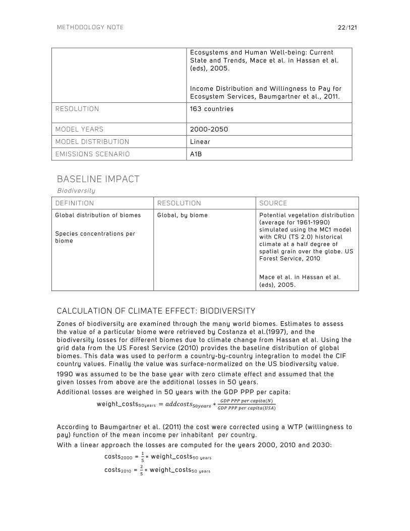
Ecosystems and Human Well-being: Current State and Trends, Mace et al. in Hassan et al. (eds), 2005.

Income Distribution and Will ingness to Pay for Ecosystem Services, Baumgartner et al. , 2011.

RESOLUTION 163 countries

MODEL YEARS 2000-2050

MODEL DISTRIBUTION Linear

EMISSIONS SCENARIO A1B

BASELINE IMPACT Biodiversity


Global distr ibution of biomes

Species concentrat ions per biome

Global, by biome Potential vegetat ion distr ibution (average for 1961-1990) simulated using the MC1 model with CRU (TS 2.0) histor ical cl imate at a half degree of spatial grain over the globe. US Forest Service, 2010

Mace et al . in Hassan et al . (eds), 2005.

CALCULATION OF CLIMATE EFFECT: BIODIVERSITY

Zones of biodiversity are examined through the many world biomes. Estimates to assess the value of a particular biome were retrieved by Costanza et al.(1997), and the biodiversity losses for different biomes due to climate change from Hassan et al. Using the grid data from the US Forest Service (2010) provides the baseline distribution of global biomes. This data was used to perform a country-by-country integration to model the CIF country values. Finally the value was surface-normalized on the US biodiversity value.

1990 was assumed to be the base year with zero climate effect and assumed that the given losses from above are the additional losses in 50 years. Additional losses are weighed in 50 years with the GDP PPP per capita:

weight_costs50yea rs = 𝑎𝑑𝑑𝑐𝑜𝑠𝑡𝑠!"!"#$% ∗!!" !!! !"# !"#$%"(!)!"# !!! !"# !"#$%"(!"#)

According to Baumgartner et al. (2011) the cost were corrected using a WTP (will ingness to pay) function of the mean income per inhabitant per country.

With a l inear approach the losses are computed for the years 2000, 2010 and 2030:

costs2000 = !!∗ weight_costs50 yea r s


METHODOLOGY NOTE

23/121


Then these costs are compared to the GDP of 2010 as follows:

CE2000 = costs2000/GDP2010 CE2010 = costs2010/GDP2010

CE2030 = costs2030/GDP2010

DESERTIFICATION

RESEARCH/DATA SOURCES: DESERTIFICATION

CLIMATE IMPACT FACTOR Desertif ication

DEFINITION Future vegetat ion distr ibution due to cl imate change.

SOURCE(S) Dangerous human-made interference with cl imate: A GISS model study, J Hansen et al , 2007

Database: Global Geospatial Potential EvapoTranspirat ion & Aridity Index Methodology and Dataset Descript ion, Trabucco and Zomer, 2009

Global data set of Monthly Irr igated and Rainfed Crop Areas around the year 2000 (MIRCA2000), version 1 .1 , Portmann et al . 2010.

Average Percent Forest Cleared Per Year, 2000-2005, by Terrestr ial Ecoregion, Hoekstra et al . , 2010

Predict ing the deforestat ion-trend under dif ferent carbon-prices, Kindermann et al . , 2006

Global Map V.1, Vegetat ion (Percent tree cover) , F Modis Data 2003. (Geospatial Information Authority of Japan, Chiba University and collaborating organizations.)

Resolution Hansen: 4° x 5° MIRCA2000: 0.5° x 0.5° Modis: 0.5°x0.5°

MODEL YEARS Base: 1961-1990; Project ion: 2070-2099


EMISSION SCENARIO IPCC SRES A1B

BASELINE IMPACT Desertif ication


METHODOLOGY NOTE

24/121

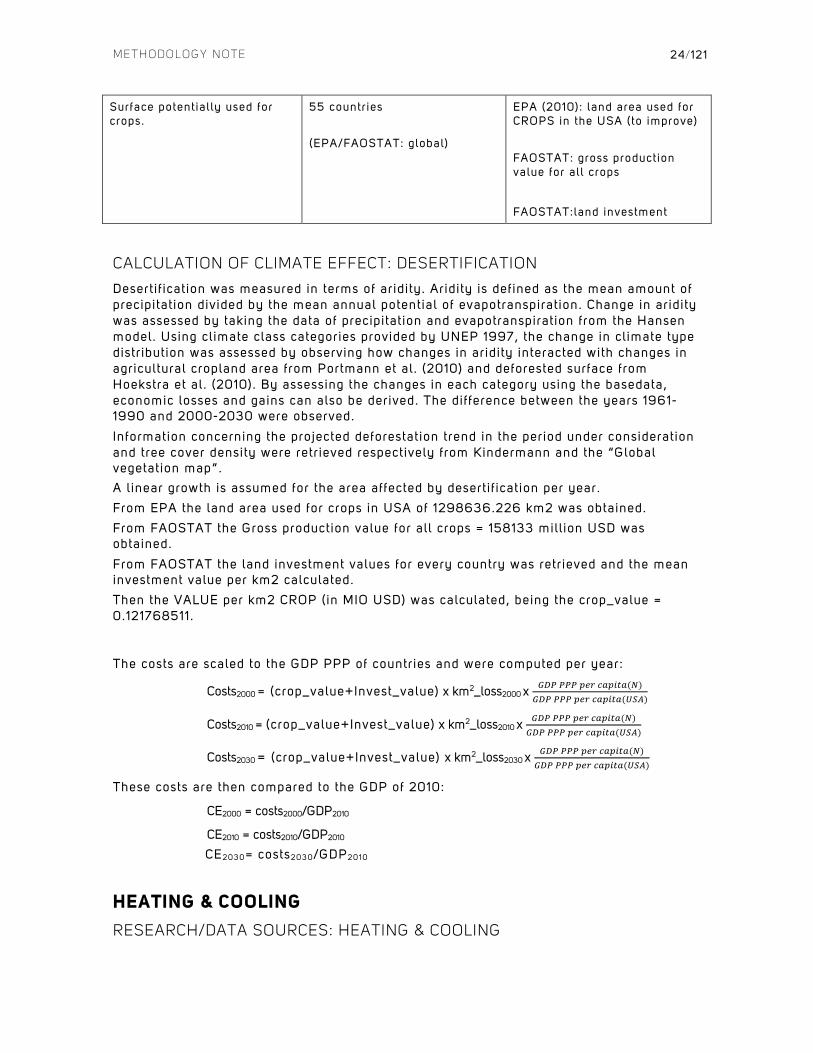
Surface potential ly used for crops.

55 countr ies

(EPA/FAOSTAT: global)

EPA (2010): land area used for CROPS in the USA (to improve)

FAOSTAT: gross production value for al l crops

FAOSTAT:land investment

CALCULATION OF CLIMATE EFFECT: DESERTIFICATION

Desertif ication was measured in terms of aridity. Aridity is defined as the mean amount of precipitation divided by the mean annual potential of evapotranspiration. Change in aridity was assessed by taking the data of precipitation and evapotranspiration from the Hansen model. Using climate class categories provided by UNEP 1997, the change in climate type distribution was assessed by observing how changes in aridity interacted with changes in agricultural cropland area from Portmann et al. (2010) and deforested surface from Hoekstra et al. (2010). By assessing the changes in each category using the basedata, economic losses and gains can also be derived. The difference between the years 1961-1990 and 2000-2030 were observed.

Information concerning the projected deforestation trend in the period under consideration and tree cover density were retrieved respectively from Kindermann and the “Global vegetation map”. A l inear growth is assumed for the area affected by desertif ication per year.

From EPA the land area used for crops in USA of 1298636.226 km2 was obtained.

From FAOSTAT the Gross production value for all crops = 158133 mill ion USD was obtained.

From FAOSTAT the land investment values for every country was retrieved and the mean investment value per km2 calculated.

Then the VALUE per km2 CROP (in MIO USD) was calculated, being the crop_value = 0.121768511.

The costs are scaled to the GDP PPP of countries and were computed per year:

Costs2000 = (crop_value+Invest_value) x km2_loss2000 x !"# !!! !"# !"#$%"(!)!"# !!! !"# !"#$%"(!"#)



These costs are then compared to the GDP of 2010:

CE2000 = costs2000/GDP2010

CE2010 = costs2010/GDP2010

CE2030= costs2030/GDP2010

HEATING & COOLING

RESEARCH/DATA SOURCES: HEATING & COOLING

METHODOLOGY NOTE

25/121

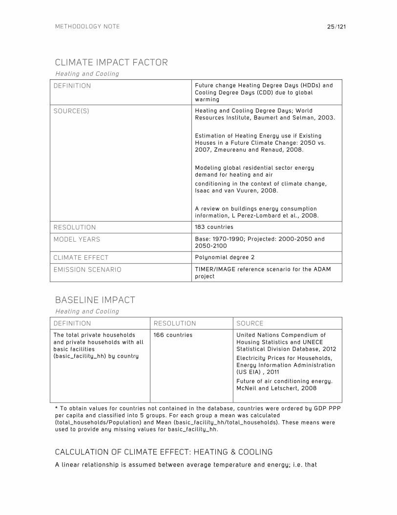
CLIMATE IMPACT FACTOR Heating and Cooling

DEFINITION Future change Heating Degree Days (HDDs) and Cooling Degree Days (CDD) due to global warming

SOURCE(S) Heating and Cooling Degree Days; World Resources Inst i tute, Baumert and Selman, 2003.

Est imation of Heating Energy use i f Exist ing Houses in a Future Cl imate Change: 2050 vs. 2007, Zmeureanu and Renaud, 2008.

Modeling global residential sector energy demand for heating and air

condit ioning in the context of cl imate change, Isaac and van Vuuren, 2008.

A review on buildings energy consumption information, L Perez-Lombard et al . , 2008.

RESOLUTION 183 countr ies

MODEL YEARS Base: 1970-1990; Projected: 2000-2050 and 2050-2100

CLIMATE EFFECT Polynomial degree 2

EMISSION SCENARIO TIMER/IMAGE reference scenario for the ADAM project

BASELINE IMPACT Heating and Cooling


The total pr ivate households and private households with all basic faci l i t ies (basic_facil i ty_hh) by country

166 countr ies

United Nations Compendium of Housing Stat ist ics and UNECE Stat ist ical Divis ion Database, 2012

Electr ic i ty Prices for Households, Energy Information Administrat ion (US EIA) , 2011

Future of air condit ioning energy. McNeil and Letschert , 2008

* To obtain values for countr ies not contained in the database, countr ies were ordered by GDP PPP per capita and classif ied into 5 groups. For each group a mean was calculated (total_households/Populat ion) and Mean (basic_facil i ty_hh/total_households) . These means were used to provide any missing values for basic_facil i ty_hh.

CALCULATION OF CLIMATE EFFECT: HEATING & COOLING

A linear relationship is assumed between average temperature and energy; i .e. that

METHODOLOGY NOTE

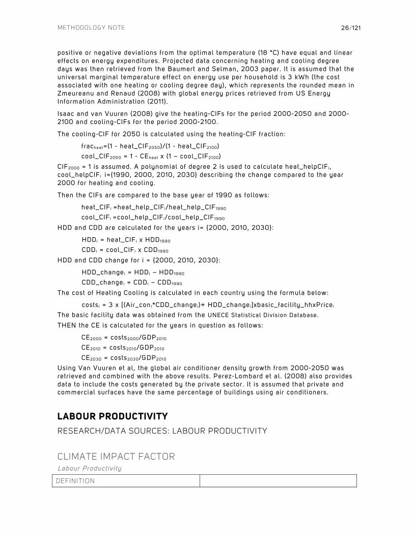
26/121

posit ive or negative deviations from the optimal temperature (18 °C) have equal and linear effects on energy expenditures. Projected data concerning heating and cooling degree days was then retrieved from the Baumert and Selman, 2003 paper. It is assumed that the universal marginal temperature effect on energy use per household is 3 kWh (the cost associated with one heating or cooling degree day), which represents the rounded mean in Zmeureanu and Renaud (2008) with global energy prices retrieved from US Energy Information Administration (2011).

Isaac and van Vuuren (2008) give the heating-CIFs for the period 2000-2050 and 2000-2100 and cooling-CIFs for the period 2000-2100.

The cooling-CIF for 2050 is calculated using the heating-CIF fraction:

frachea t=(1 - heat_CIF2050)/(1 - heat_CIF2100) cool_CIF2050 = 1 - CEhea t x (1 – cool_CIF2100)

CIF2000 = 1 is assumed. A polynomial of degree 2 is used to calculate heat_helpCIFi, cool_helpCIFi i={1990, 2000, 2010, 2030} describing the change compared to the year 2000 for heating and cooling.

Then the CIFs are compared to the base year of 1990 as follows:

heat_CIFi =heat_help_CIFi/heat_help_CIF1990

cool_CIFi =cool_help_CIFi/cool_help_CIF1990

HDD and CDD are calculated for the years i= {2000, 2010, 2030}:

HDDi = heat_CIFi x HDD1990 CDDi = cool_CIFi x CDD1990

HDD and CDD change for i = {2000, 2010, 2030}:

HDD_changei = HDDi – HDD1990 CDD_changei = CDDi – CDD1990

The cost of Heating Cooling is calculated in each country using the formula below:

costs i = 3 x [(Air_coni*CDD_changei)+ HDD_changei]xbasic_facil i ty_hhxPricei The basic facil i ty data was obtained from the UNECE Statist ical Divis ion Database.

THEN the CE is calculated for the years in question as follows:


CE2030 = costs2030/GDP2010

Using Van Vuuren et al, the global air conditioner density growth from 2000-2050 was retrieved and combined with the above results. Perez-Lombard et al. (2008) also provides data to include the costs generated by the private sector. I t is assumed that private and commercial surfaces have the same percentage of buildings using air conditioners.

LABOUR PRODUCTIVITY

RESEARCH/DATA SOURCES: LABOUR PRODUCTIVITY

CLIMATE IMPACT FACTOR Labour Productivity

DEFINITION

METHODOLOGY NOTE

27/121

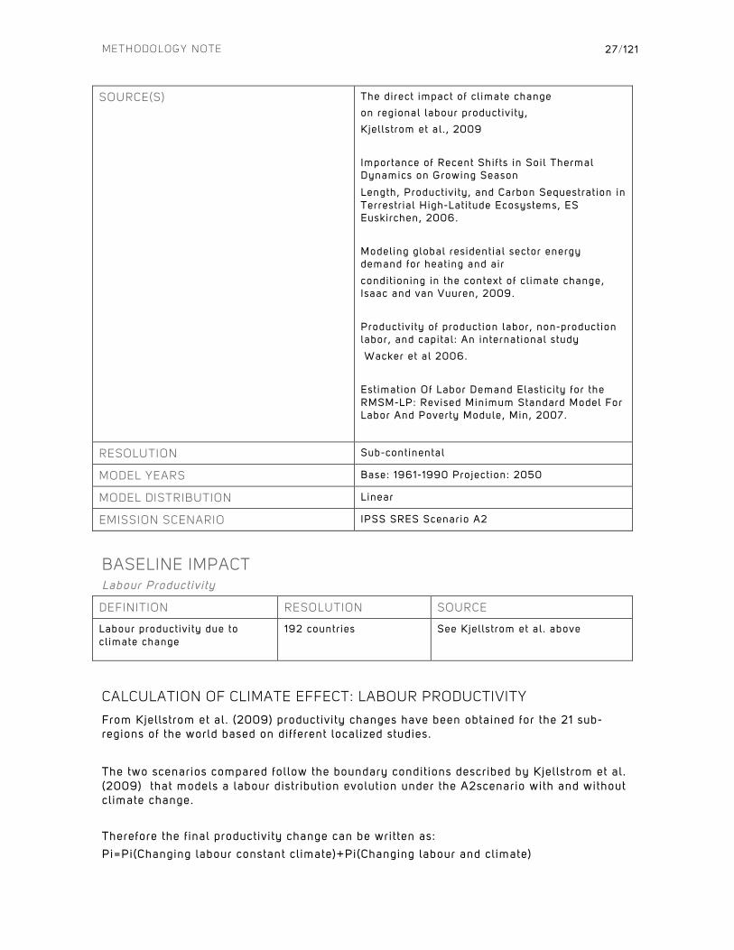
SOURCE(S) The direct impact of cl imate change

on regional labour productivi ty,

Kjellstrom et al . , 2009

Importance of Recent Shif ts in Soil Thermal Dynamics on Growing Season

Length, Productivi ty, and Carbon Sequestrat ion in Terrestr ial High-Lati tude Ecosystems, ES Euskirchen, 2006.

Modeling global residential sector energy demand for heating and air

condit ioning in the context of cl imate change, Isaac and van Vuuren, 2009.

Productivi ty of production labor, non-production labor, and capital : An international study

Wacker et al 2006.

Est imation Of Labor Demand Elast ic i ty for the RMSM-LP: Revised Minimum Standard Model For Labor And Poverty Module, Min, 2007.

RESOLUTION Sub-continental

MODEL YEARS Base: 1961-1990 Project ion: 2050


EMISSION SCENARIO IPSS SRES Scenario A2

BASELINE IMPACT Labour Productivity


Labour productivi ty due to cl imate change

192 countr ies See Kjellstrom et al . above

CALCULATION OF CLIMATE EFFECT: LABOUR PRODUCTIVITY

From Kjellstrom et al. (2009) productivity changes have been obtained for the 21 sub- regions of the world based on different localized studies.

The two scenarios compared follow the boundary conditions described by Kjellstrom et al. (2009) that models a labour distribution evolution under the A2scenario with and without climate change.

Therefore the final productivity change can be written as: Pi=Pi(Changing labour constant climate)+Pi(Changing labour and climate)

METHODOLOGY NOTE

28/121

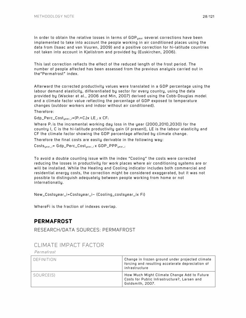
In order to obtain the relative losses in terms of GDPyear several corrections have been implemented to take into account the people working in air conditioned places using the data from (Isaac and van Vuuren, 2009) and a posit ive correction for hi-latitude countries not taken into account in Kjellstrom and provided by (Euskirchen, 2006).

This last correction reflects the effect of the reduced length of the frost period. The number of people affected has been assessed from the previous analysis carried out in the“Permafrost” index.

Afterward the corrected productivity values were translated in a GDP percentage using the labour demand elasticity, differentiated by sector for every country, using the data provided by (Wacker et al. , 2006 and Min, 2007) derived using the Cobb-Douglas model and a climate factor value reflecting the percentage of GDP exposed to temperature changes (outdoor workers and indoor without air conditioned).

Therefore:

Gdp_Perc_Costyear_ i=(Pi+Ci)x LE_i x CFi

Where Pi is the incremental working day loss in the year (2000,2010,2030) for the country I, C is the hi-latitude productivity gain (if present), LE is the labour elasticity and CF the climate factor showing the GDP percentage affected by climate change. Therefore the final costs are easily derivable in the following way:

Costsyear_ i= Gdp_Perc_Costyea r_ i x GDP_PPPyear_ i

To avoid a double counting issue with the index “Cooling” the costs were corrected reducing the losses in productivity for work places where air conditioning systems are or will be installed. While the Heating and Cooling indicator includes both commercial and residential energy costs, the correction might be considered exaggerated, but it was not possible to distinguish adequately between people working from home or not internationally.

New_Costsyear_i=Costsyear_i– (Cooling_costsyear_ix Fi)

WhereFi is the fraction of indexes overlap.

PERMAFROST

RESEARCH/DATA SOURCES: PERMAFROST

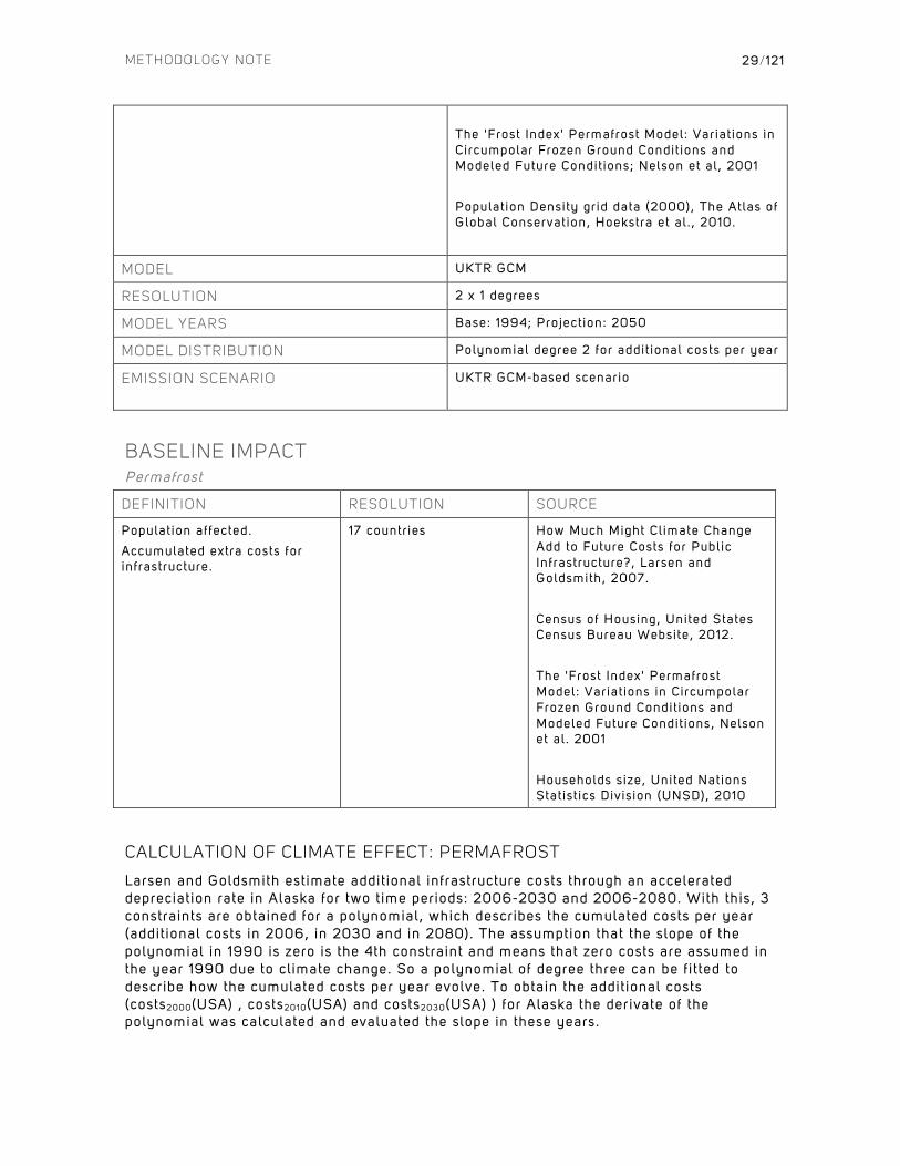
CLIMATE IMPACT FACTOR Permafrost

DEFINITION Change in frozen ground under projected cl imate forcing and result ing accelerate depreciat ion of infrastructure

SOURCE(S) How Much Might Cl imate Change Add to Future Costs for Public Infrastructure?, Larsen and Goldsmith, 2007.

METHODOLOGY NOTE

29/121

The 'Frost Index' Permafrost Model: Variat ions in Circumpolar Frozen Ground Condit ions and Modeled Future Condit ions; Nelson et al , 2001

Populat ion Density grid data (2000), The Atlas of Global Conservation, Hoekstra et al . , 2010.

MODEL UKTR GCM

RESOLUTION 2 x 1 degrees

MODEL YEARS Base: 1994; Project ion: 2050

MODEL DISTRIBUTION Polynomial degree 2 for addit ional costs per year

EMISSION SCENARIO UKTR GCM-based scenario

BASELINE IMPACT Permafrost


Population affected.

Accumulated extra costs for infrastructure.

17 countr ies How Much Might Cl imate Change Add to Future Costs for Public Infrastructure?, Larsen and Goldsmith, 2007.

Census of Housing, United States Census Bureau Website, 2012.

The 'Frost Index' Permafrost Model: Variat ions in Circumpolar Frozen Ground Condit ions and Modeled Future Condit ions, Nelson et al . 2001

Households size, United Nations Stat ist ics Divis ion (UNSD), 2010

CALCULATION OF CLIMATE EFFECT: PERMAFROST

Larsen and Goldsmith estimate additional infrastructure costs through an accelerated depreciation rate in Alaska for two time periods: 2006-2030 and 2006-2080. With this, 3 constraints are obtained for a polynomial, which describes the cumulated costs per year (additional costs in 2006, in 2030 and in 2080). The assumption that the slope of the polynomial in 1990 is zero is the 4th constraint and means that zero costs are assumed in the year 1990 due to climate change. So a polynomial of degree three can be fitted to describe how the cumulated costs per year evolve. To obtain the additional costs (costs2000(USA) , costs2010(USA) and costs2030(USA) ) for Alaska the derivate of the polynomial was calculated and evaluated the slope in these years.

METHODOLOGY NOTE

30/121

With respect to the populations affected (16 countries), the model output from F.E. Nelson et al provides the number of affected people by permafrost in 2050 for country N (affected(N)). This is taken as constant in order that impacts from climate change would not be inadvertently derived from population growth.

From the UNSD household sizes for the country N was retrieved.

Costs due to the private sector were also calculated, taking into account the population affected, the mean household size and the mean property value obtained from the US Census Bureau for Alaska. The costs from both the private and public sector were then added to give total costs, which were extrapolated to affected countries on a GDP PPP and population basis for affected areas.

To calculate the costs for the different countries N we used the given costs, the affected people and the GDP PPP per capita 2010 of Alaska (USA) and the number of affected people and their GDP PPP per capita 2010 of country N:

K(N)=(household_size_USA/household_size_country_N)

costs2000(N)= costs2000(USA) ∗ [!""#$%#&(!)∗!"#_!!!!"#"(!)][!""#$%#&(!"#)∗!"#_!!!!"#"(!"#)]

x K(N)

costs2010(N)= costs2010(USA) ∗ [!""#$%#&(!)∗!"#_!!!!"#"(!)][!""#$%#&(!"#)∗!"#_!!!!"#"(!"#)]

x K(N)

costs2030(N)= costs2030(USA) ∗ [!""#$%#&(!)∗!"#_!!!!"#"(!)][!""#$%#&(!"#)∗!"#_!!!!"#"(!"#)]

x K(N)

Then we compare these costs to the GDP of 2010:


CE2030 = costs2030/GDP2010

SEA-LEVEL RISE

RESEARCH/DATA SOURCES: SEA-LEVEL RISE

CLIMATE IMPACT FACTOR Sea-Level Rise

DEFINITION Costs due to cl imate change-induced sea-level r ise for coastal zones (Change in t idal basin nourishment costs, beach nourishment costs, land loss costs, migrat ion costs, r iver f lood costs, sal inity intrusion costs, sea dike costs, sea f lood costs and wetland nourishment costs due to cl imate change).

SOURCE(S) Dynamic Interactive Vulnerabil i ty Assessment, DIVA 2003, DINAS-COAST 2003

RESOLUTION 147 Countr ies


CLIMATE EFFECT SLR_Tidal_basin_nourishment_costs_2010=SLR_

METHODOLOGY NOTE

31/121

Tidal_basin_nourishment_costs_2010/GDP_2010_Country

SLR2010_index = ((SLR_Adaptcost_PERGDP_2010/(SLR_MEAN_DEV_MEAN*10))+1)*100

EMISSION SCENARIO A1FI

BASELINE IMPACT Sea-Level Rise


Cost of sea level r ise 147 Countr ies DIVA, 2003

CALCULATION OF CLIMATE EFFECT: SEA-LEVEL RISE

The comprehensive DIVA model provides cost outputs for different factors and timeframes autonomously generating a Climate Effect for sea-level r ise. Cost data for the ten different variables provided by the DIVA program are used as follows:

Total_costs = Tidal_basin_nourishment_costs + Beach_nourishment_costs + Land_loss_costs + Migration_costs + River_dike_costs+ River_flood_costs+ Salinity_intrusion_costs + Sea_dike_costs+ Sea_flood_costs+ Wetland_nourishment_costs

These costs were then compared to the GDP of 2010:

CE2000 = costs2000/GDP2010


WATER

RESEARCH/DATA SOURCES: WATER

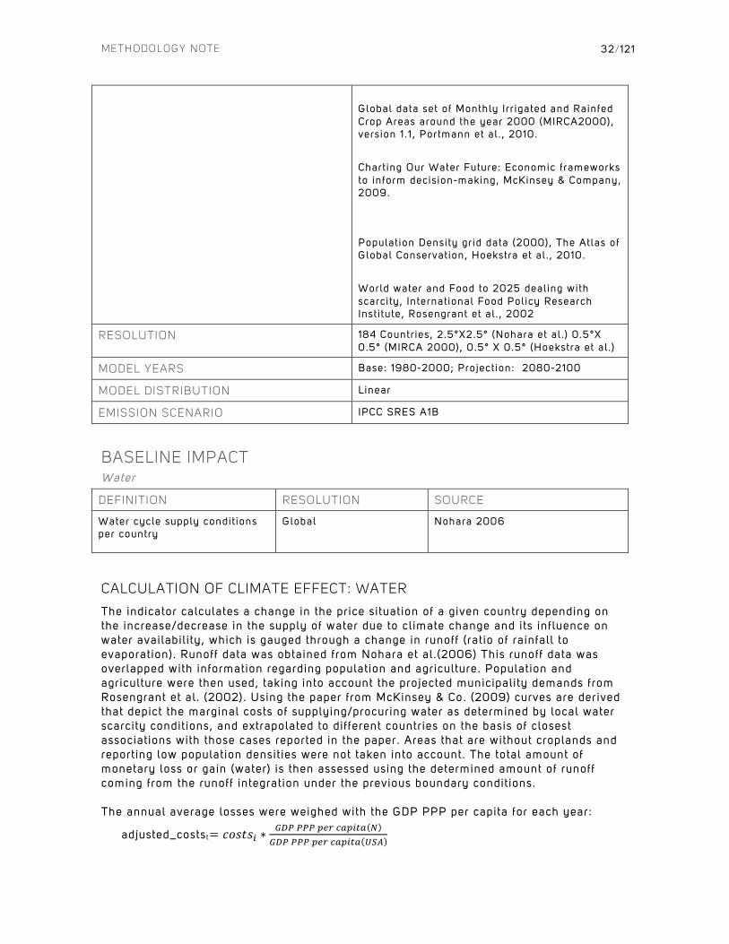
CLIMATE IMPACT FACTOR Water

DEFINITION Marginal (adaptat ion) costs for replacing water losses due to cl imate change adjusted for local market condit ions/scarcity.

SOURCE(S)

Impact of Cl imate Change on River Discharge Projected by Mult imodel Ensemble, Nohara et al . , 2006.

METHODOLOGY NOTE

32/121

Global data set of Monthly Irr igated and Rainfed Crop Areas around the year 2000 (MIRCA2000), version 1 .1 , Portmann et al . , 2010.

Chart ing Our Water Future: Economic frameworks to inform decision-making, McKinsey & Company, 2009.


World water and Food to 2025 dealing with scarcity, International Food Policy Research Inst i tute, Rosengrant et al . , 2002

RESOLUTION 184 Countr ies, 2.5°X2.5° (Nohara et al . ) 0.5°X 0.5° (MIRCA 2000), 0.5° X 0.5° (Hoekstra et al . )

MODEL YEARS Base: 1980-2000; Project ion: 2080-2100



BASELINE IMPACT Water


Water cycle supply condit ions per country

Global Nohara 2006

CALCULATION OF CLIMATE EFFECT: WATER

The indicator calculates a change in the price situation of a given country depending on the increase/decrease in the supply of water due to climate change and its influence on water availabil ity, which is gauged through a change in runoff (ratio of rainfall to evaporation). Runoff data was obtained from Nohara et al. (2006) This runoff data was overlapped with information regarding population and agriculture. Population and agriculture were then used, taking into account the projected municipality demands from Rosengrant et al. (2002). Using the paper from McKinsey & Co. (2009) curves are derived that depict the marginal costs of supplying/procuring water as determined by local water scarcity conditions, and extrapolated to different countries on the basis of closest associations with those cases reported in the paper. Areas that are without croplands and reporting low population densities were not taken into account. The total amount of monetary loss or gain (water) is then assessed using the determined amount of runoff coming from the runoff integration under the previous boundary conditions. The annual average losses were weighed with the GDP PPP per capita for each year:

adjusted_costst= 𝑐𝑜𝑠𝑡𝑠! ∗!"# !!! !"# !"#$%" !!"# !!! !"# !"#$%" !"#

METHODOLOGY NOTE

33/121

Then these costs were compared to the GDP of 2010:

CE2000 = adjusted_costs2000/GDP2010 CE2010 = adjusted_costs2010/GDP2010 CE2030 = adjusted_costs2030/GDP2010

METHODOLOGY NOTE

34/121

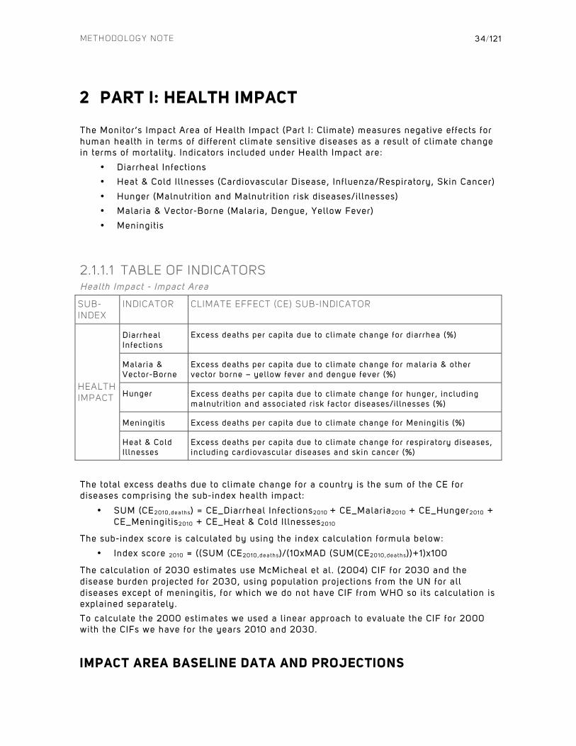
2 PART I: HEALTH IMPACT

The Monitor’s Impact Area of Health Impact (Part I : Climate) measures negative effects for human health in terms of different climate sensit ive diseases as a result of climate change in terms of mortality. Indicators included under Health Impact are:

• Diarrheal Infections

• Heat & Cold Il lnesses (Cardiovascular Disease, Influenza/Respiratory, Skin Cancer)

• Hunger (Malnutrit ion and Malnutrit ion risk diseases/illnesses)

• Malaria & Vector-Borne (Malaria, Dengue, Yellow Fever)

• Meningitis

2.1.1.1 TABLE OF INDICATORS Health Impact - Impact Area

SUB-INDEX

INDICATOR CLIMATE EFFECT (CE) SUB-INDICATOR

HEALTH IMPACT

Diarrheal Infect ions

Excess deaths per capita due to cl imate change for diarrhea (%)

Malaria & Vector-Borne

Excess deaths per capita due to cl imate change for malaria & other vector borne – yellow fever and dengue fever (%)

Hunger Excess deaths per capita due to cl imate change for hunger, including malnutr i t ion and associated r isk factor diseases/i l lnesses (%)

Meningit is Excess deaths per capita due to cl imate change for Meningit is (%)

Heat & Cold I l lnesses

Excess deaths per capita due to cl imate change for respiratory diseases, including cardiovascular diseases and skin cancer (%)

The total excess deaths due to climate change for a country is the sum of the CE for diseases comprising the sub-index health impact:

• SUM (CE2010 ,dea ths) = CE_Diarrheal Infections2010 + CE_Malaria2010 + CE_Hunger2010 + CE_Meningitis2010 + CE_Heat & Cold Il lnesses2010


• Index score 2010 = ((SUM (CE2010 ,dea ths)/(10xMAD (SUM(CE2010 ,dea ths) )+1)x100

The calculation of 2030 estimates use McMicheal et al. (2004) CIF for 2030 and the disease burden projected for 2030, using population projections from the UN for all diseases except of meningitis, for which we do not have CIF from WHO so its calculation is explained separately.

To calculate the 2000 estimates we used a l inear approach to evaluate the CIF for 2000 with the CIFs we have for the years 2010 and 2030.


METHODOLOGY NOTE

35/121

SOCIOECONOMIC BASELINE Health Impact


Population (per country) divided by 1000

By country UN Population Division - Medium-fert i l i ty variant, 2010-2100

SOCIOECONOMIC PROJECTION Health Impact

DEFINITION RESOLUTION SCENARIO SOURCE


By country UN Stat Populat ion (per country) divided by 1000

RESEARCH/DATA SOURCES: HEALTH IMPACT

CLIMATE IMPACT FACTOR Health Impact (All Indicators except meningitis, heat & cold il lnesses)

DEFINITION Marginal mortal i ty due to cl imate change for a range of cl imate sensit ive diseases

SOURCE(S) WHO

MODEL Comparative Quanti f icat ion of Health Risks, Global and Regional Burden of Disease Attr ibutable to Selected Major Risk Factors McMichael et al in Ezzati et al (eds.) ,WHO, 2004

EMISSION SCENARIO IPCC S750

RESOLUTION By WHO sub-region

MODEL YEARS Base: 2004; Project ion: 2000, 2010, 2030

MODEL DISTRIBUTION -

BASELINE IMPACT Health Impact (All Indicators)


Total deaths divided by 1000 for the year 2008

Global, by country (193 countr ies)

Global Burden of Disease Study Apri l 2011, WHO* (WHO BDD)

*2004 database for Yellow Fever: Yellow fever is the only disease with no updated data for the year 2008, so the similar but year 2004 database from WHO is drawn upon instead.

METHODOLOGY NOTE

36/121

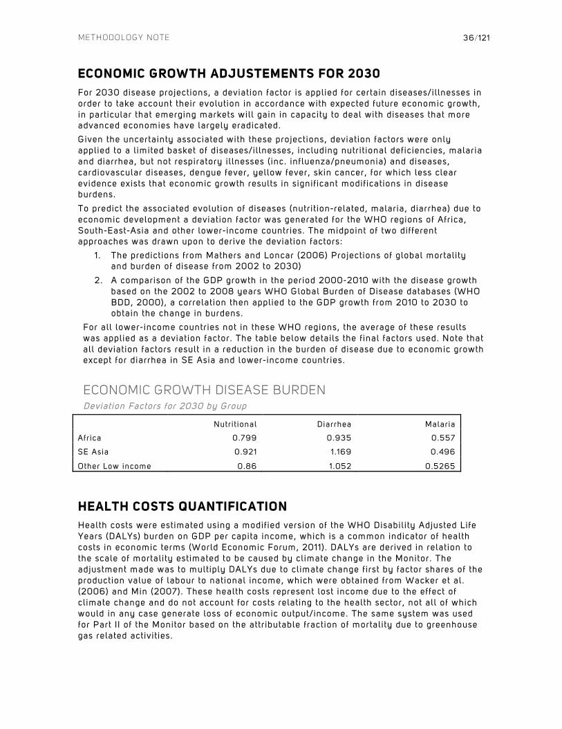
ECONOMIC GROWTH ADJUSTEMENTS FOR 2030

For 2030 disease projections, a deviation factor is applied for certain diseases/illnesses in order to take account their evolution in accordance with expected future economic growth, in particular that emerging markets will gain in capacity to deal with diseases that more advanced economies have largely eradicated.

Given the uncertainty associated with these projections, deviation factors were only applied to a l imited basket of diseases/illnesses, including nutrit ional deficiencies, malaria and diarrhea, but not respiratory il lnesses (inc. influenza/pneumonia) and diseases, cardiovascular diseases, dengue fever, yellow fever, skin cancer, for which less clear evidence exists that economic growth results in signif icant modifications in disease burdens.

To predict the associated evolution of diseases (nutrit ion-related, malaria, diarrhea) due to economic development a deviation factor was generated for the WHO regions of Africa, South-East-Asia and other lower-income countries. The midpoint of two different approaches was drawn upon to derive the deviation factors:

1 . The predictions from Mathers and Loncar (2006) Projections of global mortality and burden of disease from 2002 to 2030)

2. A comparison of the GDP growth in the period 2000-2010 with the disease growth based on the 2002 to 2008 years WHO Global Burden of Disease databases (WHO BDD, 2000), a correlation then applied to the GDP growth from 2010 to 2030 to obtain the change in burdens.

For all lower-income countries not in these WHO regions, the average of these results was applied as a deviation factor. The table below details the final factors used. Note that all deviation factors result in a reduction in the burden of disease due to economic growth except for diarrhea in SE Asia and lower-income countries.

ECONOMIC GROWTH DISEASE BURDEN Deviation Factors for 2030 by Group

Nutr i t ional Diarrhea Malaria

Afr ica 0.799 0.935 0.557

SE Asia 0.921 1 .169 0.496

Other Low income 0.86 1.052 0.5265

HEALTH COSTS QUANTIFICATION

Health costs were estimated using a modified version of the WHO Disabil ity Adjusted Life Years (DALYs) burden on GDP per capita income, which is a common indicator of health costs in economic terms (World Economic Forum, 2011). DALYs are derived in relation to the scale of mortality estimated to be caused by climate change in the Monitor. The adjustment made was to multiply DALYs due to climate change first by factor shares of the production value of labour to national income, which were obtained from Wacker et al. (2006) and Min (2007). These health costs represent lost income due to the effect of climate change and do not account for costs relating to the health sector, not all of which would in any case generate loss of economic output/income. The same system was used for Part I I of the Monitor based on the attr ibutable fraction of mortality due to greenhouse gas related activit ies.

METHODOLOGY NOTE

37/121

CALCULATION OF CLIMATE EFFECT: VECTOR-BORNE DISEASES, HUNGER AND DIARRHEAL INFECTIONS

The World Health Organization’s (WHO) 2004 “Comparative Quantif ication of Health Risk, Global and Regional Burden of Disease Attributable to Risk Factors” report, has estimated climate impact factors (CIF) for climate-sensit ive diseases at the level of WHO regions (14 sub-regions globally) derived from complex models that account for a number of different climatic influences on climate-sensit ive health disorders/diseases.

There is no CIF available for Yellow Fever or Dengue Fever in the WHO’s publication. Instead, CIFs for these well-recognized climate-sensit ive diseases are derived from the closest proxies of CIFs for other diseases. For both Yellow Fever and Dengue Fever that is Malaria, which, as a vector-borne disease, reacts to climate parameters in a comparable enough fashion to Yellow Fever and Dengue Fever to be considered an interim workable proxy.

For Hunger, the disease burden attributable to hunger-related risks calculated spans more than just mortality from nutrit ional deficiencies. It also includes an impact on diarrhea, malaria and pneumonia/respiratory infections, and measles, since hunger/malnutrit ion is a risk factor for these. WHO 2004 specif ies the impact that of climate change on health effects these diseases in two distinct ways, f irst through meteorological effects directly on the pathogens and vectors themselves, and second through an increased incidence of undernutrit ion which also increases risk of mortality to these diseases. The direct effects on pathogens and vectors themselves are captured in the relevant disease specif ic indicators of the Monitor. The hunger/undernourished-related effects are captured in the hunger indicator of the Monitor.

The climate effect (CE) is calculated by multiplying the variable (disease burden) with the CIF, as shown in the formula below: CE_Hunger2010 = (CIF_Hunger2010 ,coun t ry x Disease burden 2008,coun t ry)/Population 2010 ,con t ry

The WHO has three emission scenarios and three uncertainty scenarios resulting in a total of nine climate impact factors (CIF) per region. For the purpose of the Health Impact sub-index, the two mid-range scenarios have been applied to measure the medium expected climate change impact:

• Mid-range: “Emission reduction resulting in stabil ization at 750 ppm C02

equivalent by 2210 (s750)” • Mid-range uncertainty scenario is used “Making an adjustment for biological

adaptation” This selection results in only one impact factor being chosen per region.

The WHO CIF estimates include 2010, 2020, and 2030 estimates. It uses the HadCM2 global climate model previously used by IPCC.

CLIMATE IMPACT FACTORS

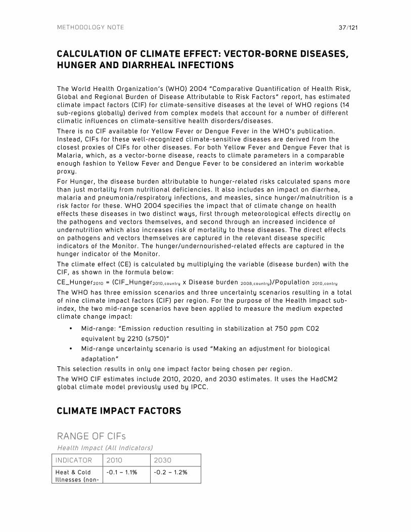
RANGE OF CIFs Health Impact (All Indicators)

INDICATOR 2010 2030

Heat & Cold I l lnesses (non-

-0.1 – 1 .1% -0.2 – 1 .2%

METHODOLOGY NOTE

38/121

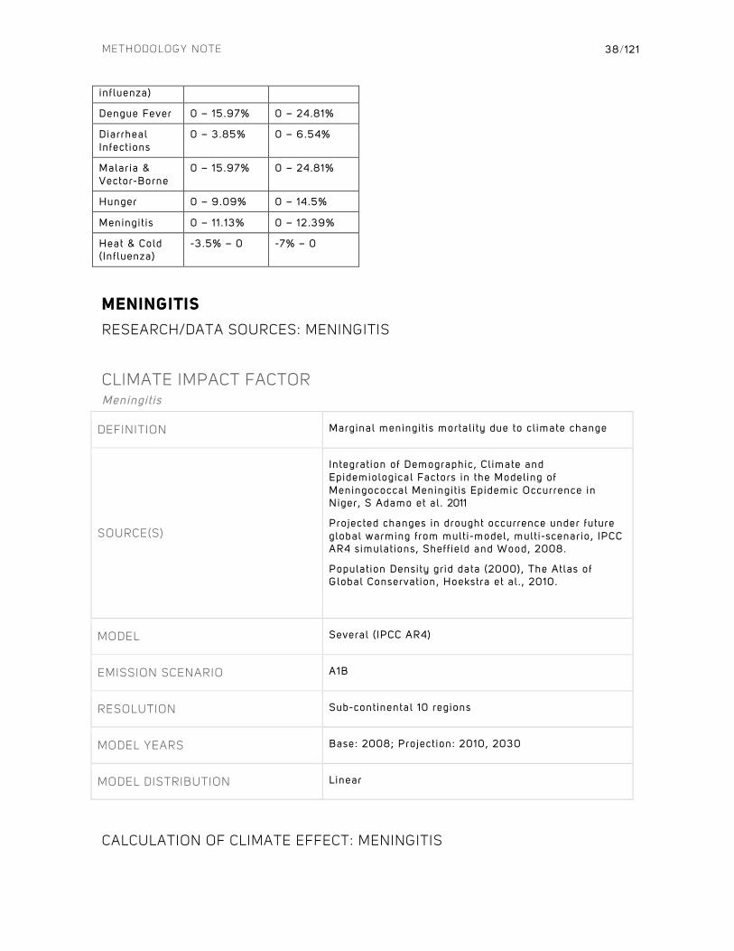
influenza)

Dengue Fever 0 – 15.97% 0 – 24.81%

Diarrheal Infect ions

0 – 3.85% 0 – 6.54%

Malaria & Vector-Borne

0 – 15.97% 0 – 24.81%

Hunger 0 – 9.09% 0 – 14.5%

Meningit is 0 – 11 .13% 0 – 12.39%

Heat & Cold ( Influenza)

-3.5% – 0 -7% – 0

MENINGITIS

RESEARCH/DATA SOURCES: MENINGITIS

CLIMATE IMPACT FACTOR Meningitis

DEFINITION Marginal meningit is mortal i ty due to cl imate change

SOURCE(S)

Integrat ion of Demographic, Cl imate and Epidemiological Factors in the Modeling of Meningococcal Meningit is Epidemic Occurrence in Niger, S Adamo et al . 2011

Projected changes in drought occurrence under future global warming from mult i-model, mult i-scenario, IPCC AR4 simulations, Sheff ield and Wood, 2008.


MODEL Several ( IPCC AR4)

EMISSION SCENARIO A1B

RESOLUTION Sub-continental 10 regions

MODEL YEARS Base: 2008; Project ion: 2010, 2030


CALCULATION OF CLIMATE EFFECT: MENINGITIS

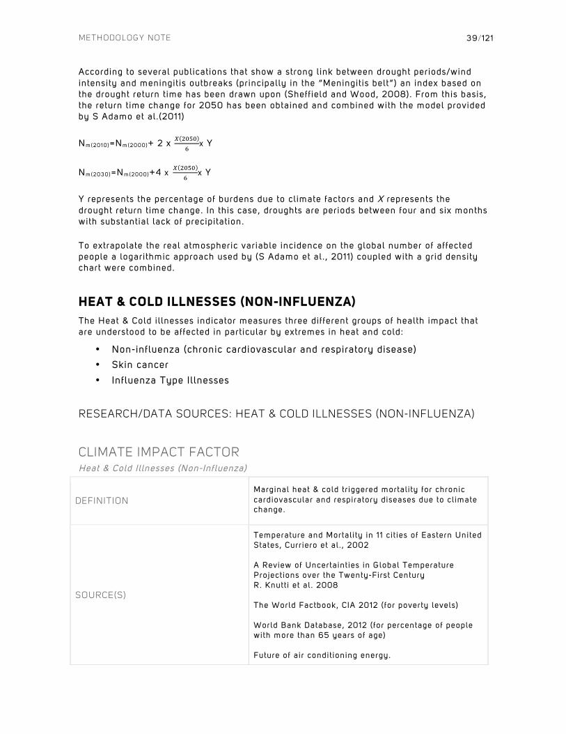
METHODOLOGY NOTE

39/121

According to several publications that show a strong link between drought periods/wind intensity and meningitis outbreaks (principally in the “Meningitis belt”) an index based on the drought return time has been drawn upon (Sheffield and Wood, 2008). From this basis, the return time change for 2050 has been obtained and combined with the model provided by S Adamo et al.(2011)

Nm(2010 )=Nm(2000)+ 2 x ! !"#"!

x Y

Nm(2030)=Nm(2000)+4 x ! !"#"!

x Y

Y represents the percentage of burdens due to climate factors and X represents the drought return time change. In this case, droughts are periods between four and six months with substantial lack of precipitation.

To extrapolate the real atmospheric variable incidence on the global number of affected people a logarithmic approach used by (S Adamo et al. , 2011) coupled with a grid density chart were combined.

HEAT & COLD ILLNESSES (NON-INFLUENZA)

The Heat & Cold il lnesses indicator measures three different groups of health impact that are understood to be affected in particular by extremes in heat and cold:

• Non-influenza (chronic cardiovascular and respiratory disease)

• Skin cancer

• Influenza Type Illnesses

RESEARCH/DATA SOURCES: HEAT & COLD ILLNESSES (NON-INFLUENZA)

CLIMATE IMPACT FACTOR Heat & Cold Il lnesses (Non-Influenza)

DEFINITION

Marginal heat & cold tr iggered mortal i ty for chronic cardiovascular and respiratory diseases due to cl imate change.

SOURCE(S)

Temperature and Mortal i ty in 11 ci t ies of Eastern United States, Curr iero et al . , 2002 A Review of Uncertaint ies in Global Temperature Project ions over the Twenty-First Century R. Knutt i et al . 2008 The World Factbook, CIA 2012 (for poverty levels) World Bank Database, 2012 (for percentage of people with more than 65 years of age) Future of air condit ioning energy.

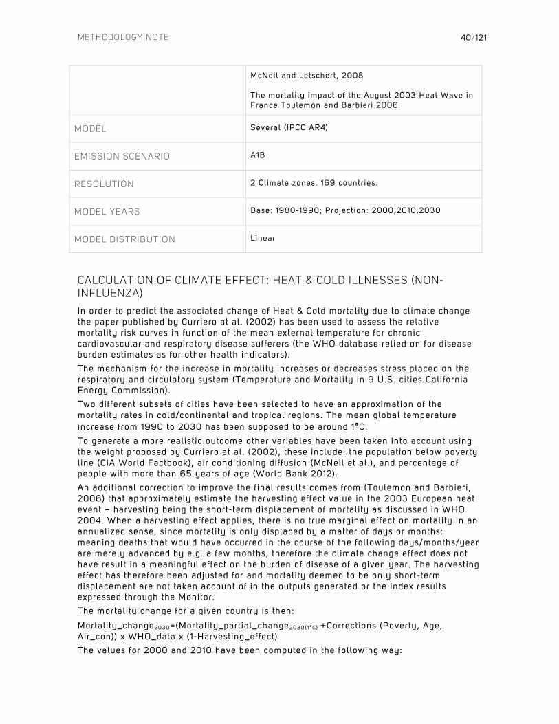
METHODOLOGY NOTE

40/121

McNeil and Letschert , 2008 The mortal i ty impact of the August 2003 Heat Wave in France Toulemon and Barbieri 2006



RESOLUTION 2 Climate zones. 169 countr ies.

MODEL YEARS Base: 1980-1990; Project ion: 2000,2010,2030


CALCULATION OF CLIMATE EFFECT: HEAT & COLD ILLNESSES (NON-INFLUENZA)

In order to predict the associated change of Heat & Cold mortality due to climate change the paper published by Curriero at al. (2002) has been used to assess the relative mortality risk curves in function of the mean external temperature for chronic cardiovascular and respiratory disease sufferers (the WHO database relied on for disease burden estimates as for other health indicators).

The mechanism for the increase in mortality increases or decreases stress placed on the respiratory and circulatory system (Temperature and Mortality in 9 U.S. cit ies California Energy Commission).

Two different subsets of cit ies have been selected to have an approximation of the mortality rates in cold/continental and tropical regions. The mean global temperature increase from 1990 to 2030 has been supposed to be around 1°C.

To generate a more realistic outcome other variables have been taken into account using the weight proposed by Curriero at al. (2002), these include: the population below poverty l ine (CIA World Factbook), air conditioning diffusion (McNeil et al. ) , and percentage of people with more than 65 years of age (World Bank 2012).

An additional correction to improve the final results comes from (Toulemon and Barbieri, 2006) that approximately estimate the harvesting effect value in the 2003 European heat event – harvesting being the short-term displacement of mortality as discussed in WHO 2004. When a harvesting effect applies, there is no true marginal effect on mortality in an annualized sense, since mortality is only displaced by a matter of days or months: meaning deaths that would have occurred in the course of the following days/months/year are merely advanced by e.g. a few months, therefore the climate change effect does not have result in a meaningful effect on the burden of disease of a given year. The harvesting effect has therefore been adjusted for and mortality deemed to be only short-term displacement are not taken account of in the outputs generated or the index results expressed through the Monitor.

The mortality change for a given country is then:

Mortality_change2030=(Mortality_partial_change2030( 1 °C ) +Corrections (Poverty, Age, Air_con)) x WHO_data x (1-Harvesting_effect)

The values for 2000 and 2010 have been computed in the following way:

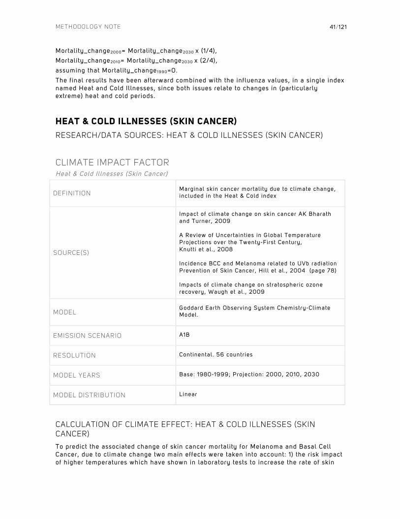
METHODOLOGY NOTE

41/121

Mortality_change2000= Mortality_change2030 x (1/4), Mortality_change2010= Mortality_change2030 x (2/4),

assuming that Mortality_change1990=0.

The final results have been afterward combined with the influenza values, in a single index named Heat and Cold Il lnesses, since both issues relate to changes in (particularly extreme) heat and cold periods.

HEAT & COLD ILLNESSES (SKIN CANCER)

RESEARCH/DATA SOURCES: HEAT & COLD ILLNESSES (SKIN CANCER)

CLIMATE IMPACT FACTOR Heat & Cold Il lnesses (Skin Cancer)

DEFINITION Marginal skin cancer mortal i ty due to cl imate change, included in the Heat & Cold index

SOURCE(S)

Impact of cl imate change on skin cancer AK Bharath and Turner, 2009 A Review of Uncertaint ies in Global Temperature Project ions over the Twenty-First Century, Knutt i et al . , 2008 Incidence BCC and Melanoma related to UVb radiat ion Prevention of Skin Cancer, Hil l et al . , 2004 (page 78) Impacts of cl imate change on stratospheric ozone recovery, Waugh et al . , 2009

MODEL Goddard Earth Observing System Chemistry-Climate Model.


RESOLUTION Continental . 56 countr ies

MODEL YEARS Base: 1980-1999; Project ion: 2000, 2010, 2030


CALCULATION OF CLIMATE EFFECT: HEAT & COLD ILLNESSES (SKIN CANCER)

To predict the associated change of skin cancer mortality for Melanoma and Basal Cell Cancer, due to climate change two main effects were taken into account: 1) the risk impact of higher temperatures which have shown in laboratory tests to increase the rate of skin

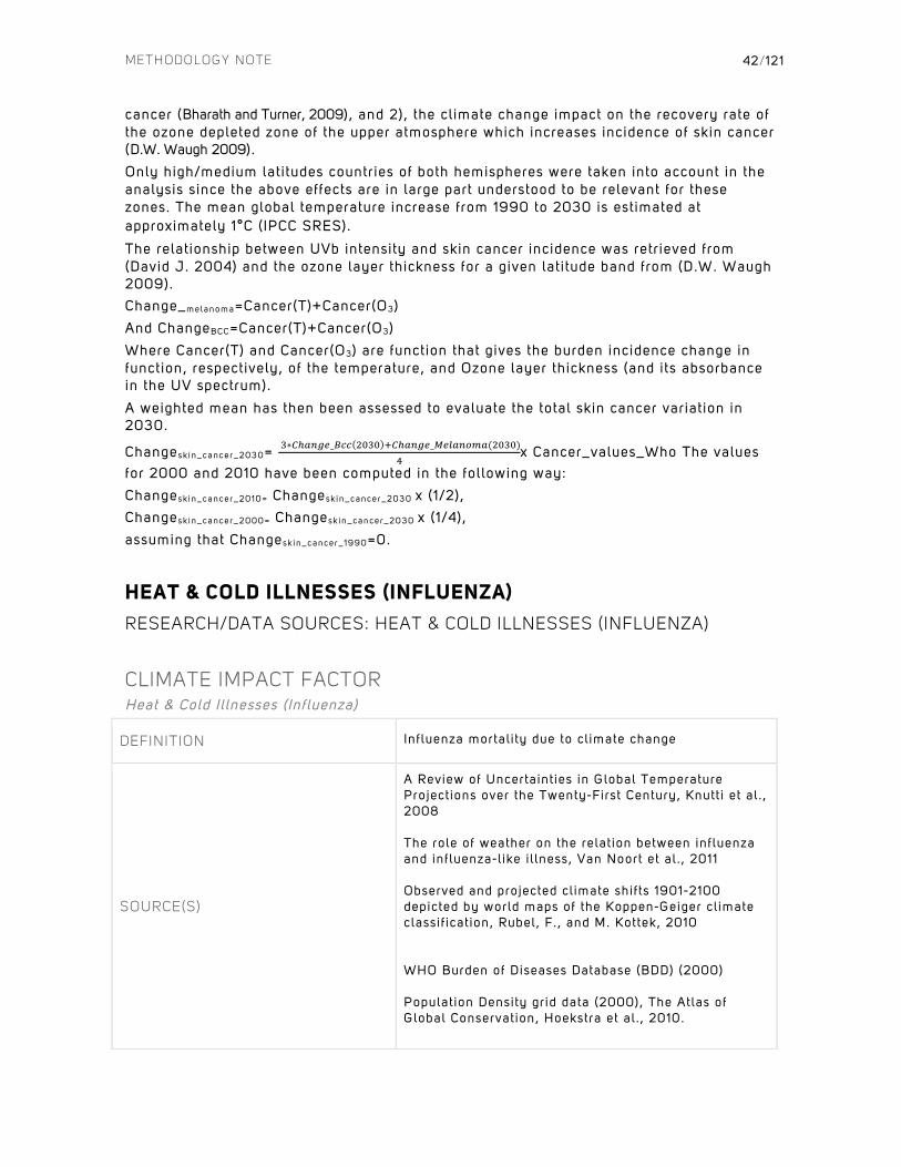
METHODOLOGY NOTE

42/121

cancer (Bharath and Turner, 2009), and 2), the climate change impact on the recovery rate of the ozone depleted zone of the upper atmosphere which increases incidence of skin cancer (D.W. Waugh 2009).

Only high/medium latitudes countries of both hemispheres were taken into account in the analysis since the above effects are in large part understood to be relevant for these zones. The mean global temperature increase from 1990 to 2030 is estimated at approximately 1°C (IPCC SRES).

The relationship between UVb intensity and skin cancer incidence was retrieved from (David J. 2004) and the ozone layer thickness for a given latitude band from (D.W. Waugh 2009). Change_melanoma=Cancer(T)+Cancer(O3)

And ChangeBCC=Cancer(T)+Cancer(O3)

Where Cancer(T) and Cancer(O3) are function that gives the burden incidence change in function, respectively, of the temperature, and Ozone layer thickness (and its absorbance in the UV spectrum).

A weighted mean has then been assessed to evaluate the total skin cancer variation in 2030.

Changesk in_cance r_2030= !∗!!!"#$_!"" !"!! !!!!"#$_!"#$%&'$(!"#")!

x Cancer_values_Who The values for 2000 and 2010 have been computed in the following way:

Changesk in_cance r_2010= Changesk in_cance r_2030 x (1/2), Changesk in_cance r_2000= Changesk in_cance r_2030 x (1/4),

assuming that Changesk in_cance r_ 1990=0.

HEAT & COLD ILLNESSES (INFLUENZA)

RESEARCH/DATA SOURCES: HEAT & COLD ILLNESSES (INFLUENZA)

CLIMATE IMPACT FACTOR Heat & Cold Il lnesses (Influenza)

DEFINITION Inf luenza mortal i ty due to cl imate change

SOURCE(S)

A Review of Uncertaint ies in Global Temperature Project ions over the Twenty-First Century, Knutt i et al . , 2008 The role of weather on the relat ion between influenza and influenza-l ike i l lness, Van Noort et al . , 2011 Observed and projected cl imate shif ts 1901-2100 depicted by world maps of the Koppen-Geiger cl imate classif icat ion, Rubel, F. , and M. Kottek, 2010 WHO Burden of Diseases Database (BDD) (2000) Populat ion Density grid data (2000), The Atlas of Global Conservation, Hoekstra et al . , 2010.

METHODOLOGY NOTE

43/121

Complicat ions of Viral Inf luenza, Rothberg et al . , 2008



RESOLUTION 2 Climate zones. 169 countr ies.

MODEL YEARS Base: 2003-2010; Project ion: 2000,2010,2030


CALCULATION OF CLIMATE EFFECT: HEAT & COLD ILLNESSES (INFLUENZA)

In order to predict the associated change of Influenza mortality due to climate change the paper published by Van Noort at al.(2012) has been used to assess the occurrence curves for influenza and influenza-like il lness (ILI) , in particular pneumonia where it cannot be easily disassociated from influenza, which is done in function of the mean external temperature.

An assumption between the ILI and influenza variation has been made in order to transpose the ILI change to the influenza one.

To reduce the complexity of the problem tropical and desert regions have been excluded, therefore the affected population has been corrected overlapping the grid population density map (Hoekstra et al . , 2010) with the Koppen climate one.

The mean global temperature increase from 1990 to 2030 is estimated at approximately 1°C (IPCC SREX).

The final results for a given country are calculated as follows:

Mortality_change2030=Percentage_change2030( 1 °C ) x R x WHO_data x P

Where R is the ratio of the country’s affected population to the total country’s population and P is an approximate percentage of influenza related mortality to the total respiratory infection deaths (WHO BDD, 2000 and Rothberg et al. 2008). The values for 2000 and 2010 have been computed in the following way:

Mortality_change2000= Mortality_change2030 x (1/4), Mortality_change2010= Mortality_change2030 x (2/4),

assuming that Mortality_change1990=0.

The final results have been afterward combined with the other non-influenza and skin cancer values, in a single index named Heat & Cold Il lnesses.

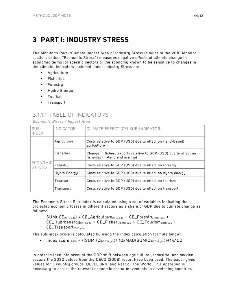
METHODOLOGY NOTE

44/121

3 PART I: INDUSTRY STRESS

The Monitor’s Part I/Climate Impact Area of Industry Stress (similar to the 2010 Monitor section, called: “Economic Stress”) measures negative effects of climate change in economic terms for specif ic sectors of the economy known to be sensit ive to changes in the climate. Indicators included under Industry Stress are:

• Agriculture

• Fisheries

• Forestry

• Hydro Energy

• Tourism

• Transport

3.1.1.1 TABLE OF INDICATORS Economic Stress - Impact Area

SUB-INDEX

INDICATOR CLIMATE EFFECT (CE) SUB-INDICATOR

ECONOMIC STRESS

Agriculture Costs relat ive to GDP (USD) due to effect on ( land-based) agriculture

Fisheries Change in f ishery exports relat ive to GDP (USD) due to effect on f isheries ( in-land and marine)

Forestry Costs relat ive to GDP (USD) due to effect on forestry

Hydro Energy Costs relat ive to GDP (USD) due to effect on hydro energy

Tourism Costs relat ive to GDP (USD) due to effect on tourism

Transport Costs relat ive to GDP (USD) due to effect on transport

The Economic Stress Sub-index is calculated using a set of variables indicating the projected economic losses in different sectors as a share of GDP due to climate change as follows:

• SUM( CE2010 ,gdp) = CE_Agriculture2010 ,gdp + CE_Forestry2010 ,gdp + CE_Hydroenergy2010 ,gdp + CE_Fishery2010 ,gdp + CE_Tourism2010 ,gdp + CE_Transport2010 ,gdp


• Index score 2010 = ((SUM (CE2010 ,gdp)/(10xMAD(SUM(CE2010 ,gdp))+1)x100

In order to take into account the GDP shift between agricultural, industrial and service sectors the 2030 values from the OECD (2008) report have been used. The paper gives values for 3 country groups: OECD, BRIC and Rest of The World. This operation is necessary to assess the relevant economic sector movements in developing countries.

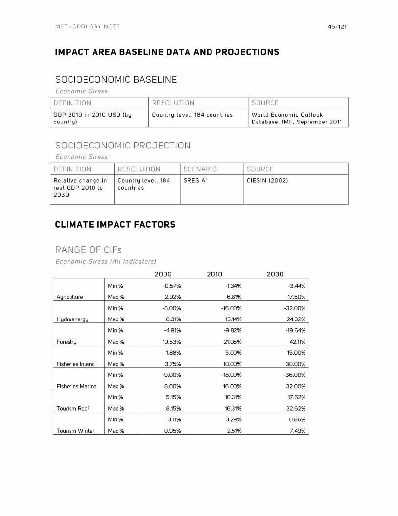
METHODOLOGY NOTE

45/121


SOCIOECONOMIC BASELINE Economic Stress



Country level, 184 countr ies World Economic Outlook Database, IMF, September 2011

SOCIOECONOMIC PROJECTION Economic Stress




SRES A1 CIESIN (2002)


RANGE OF CIFs Economic Stress (All Indicators)

2000 2010 2030

Agriculture

Min % -0.57% -1.34% -3.44%

Max % 2.92% 6.81% 17.50%

Hydroenergy

Min % -8.00% -16.00% -32.00%

Max % 8.31% 15.14% 24.32%

Forestry

Min % -4.91% -9.82% -19.64%

Max % 10.53% 21.05% 42.11%

Fisheries Inland

Min % 1.88% 5.00% 15.00%

Max % 3.75% 10.00% 30.00%

Fisheries Marine

Min % -9.00% -18.00% -36.00%

Max % 8.00% 16.00% 32.00%

Tourism Reef

Min % 5.15% 10.31% 17.62%

Max % 8.15% 16.31% 32.62%

Tourism Winter

Min % 0.11% 0.29% 0.86%

Max % 0.95% 2.51% 7.49%

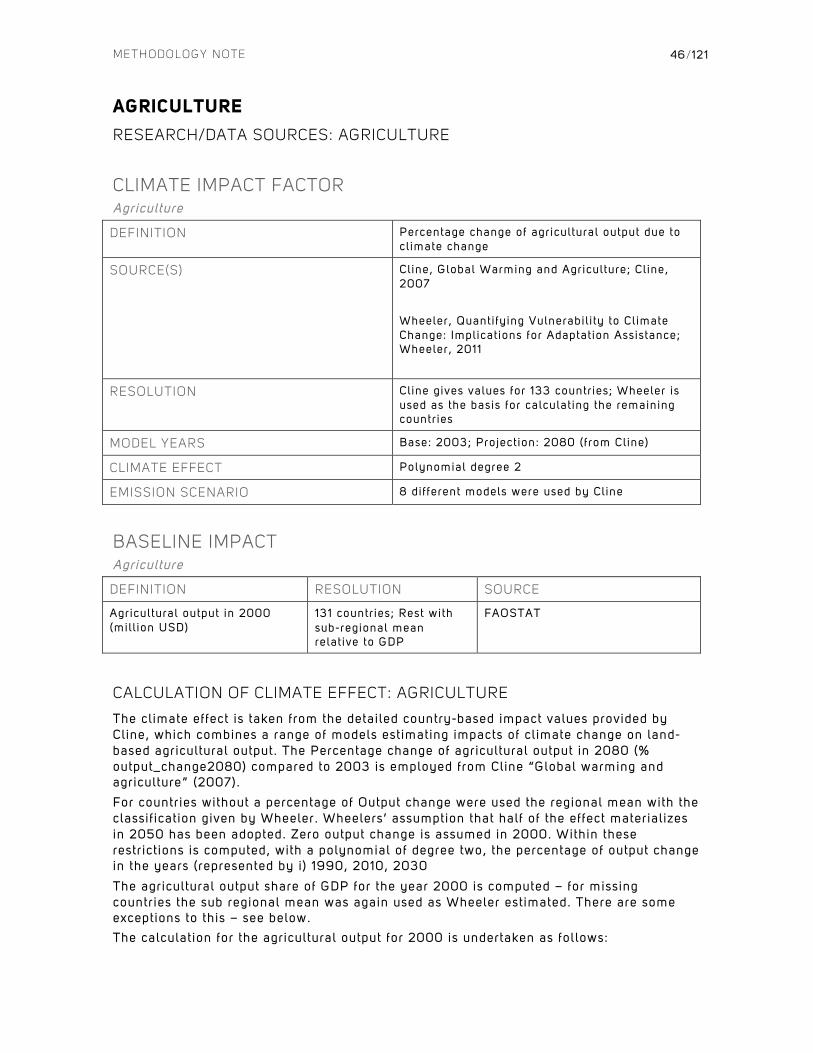
METHODOLOGY NOTE

46 /121

AGRICULTURE

RESEARCH/DATA SOURCES: AGRICULTURE

CLIMATE IMPACT FACTOR Agriculture

DEFINITION Percentage change of agricultural output due to cl imate change

SOURCE(S) Cline, Global Warming and Agriculture; Cl ine, 2007

Wheeler, Quanti fying Vulnerabil i ty to Cl imate Change: Implicat ions for Adaptat ion Assistance; Wheeler, 2011

RESOLUTION Cline gives values for 133 countr ies; Wheeler is used as the basis for calculat ing the remaining countr ies

MODEL YEARS Base: 2003; Project ion: 2080 (from Cline)

CLIMATE EFFECT Polynomial degree 2

EMISSION SCENARIO 8 dif ferent models were used by Cline

BASELINE IMPACT Agriculture


Agricultural output in 2000 (mil l ion USD)

131 countr ies; Rest with sub-regional mean relat ive to GDP

FAOSTAT

CALCULATION OF CLIMATE EFFECT: AGRICULTURE

The climate effect is taken from the detailed country-based impact values provided by Cline, which combines a range of models estimating impacts of climate change on land-based agricultural output. The Percentage change of agricultural output in 2080 (% output_change2080) compared to 2003 is employed from Cline “Global warming and agriculture” (2007).

For countries without a percentage of Output change were used the regional mean with the classif ication given by Wheeler. Wheelers’ assumption that half of the effect materializes in 2050 has been adopted. Zero output change is assumed in 2000. Within these restrictions is computed, with a polynomial of degree two, the percentage of output change in the years (represented by i) 1990, 2010, 2030

The agricultural output share of GDP for the year 2000 is computed – for missing countries the sub regional mean was again used as Wheeler estimated. There are some exceptions to this – see below. The calculation for the agricultural output for 2000 is undertaken as fol lows:

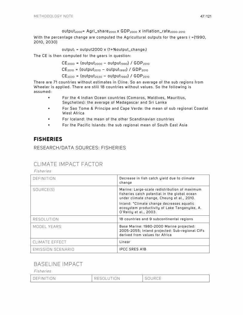
METHODOLOGY NOTE

47/121

output2000= Agri_share2000 x GDP2000 x inflation_rate2000-2010

With the percentage change are computed the Agricultural outputs for the years i ={1990, 2010, 2030}

output i = output2000 x (1+%output_changei)

The CE is then computed for the years in question:

CE2000 = (output2000 – output1990) / GDP2010



There are 71 countries without estimates in Cline. So an average of the sub regions from Wheeler is applied. There are sti l l 18 countries without values. So the following is assumed:

• For the 4 Indian Ocean countries (Comoros, Maldives, Maurit ius, Seychelles): the average of Madagascar and Sri Lanka

• For Sao Tome & Principe and Cape Verde: the mean of sub regional Coastal West Africa

• For Iceland: the mean of the other Scandinavian countries • For the Pacific Islands: the sub regional mean of South East Asia

FISHERIES

RESEARCH/DATA SOURCES: FISHERIES

CLIMATE IMPACT FACTOR Fisheries

DEFINITION Decrease in f ish catch yield due to cl imate change

SOURCE(S) Marine: Large-scale redistr ibution of maximum fisheries catch potential in the global ocean under cl imate change, Cheung et al . , 2010.

Inland: “Climate change decreases aquatic ecosystem productivi ty of Lake Tanganyike, A. O´Reil ly et al . , 2003.

RESOLUTION 18 countr ies and 9 subcontinental regions

MODEL YEARS Base Marine: 1980-2000 Marine projected: 2005-2055; Inland projected: Sub-regional CIFs derived from values for Afr ica

CLIMATE EFFECT Linear


BASELINE IMPACT Fisheries


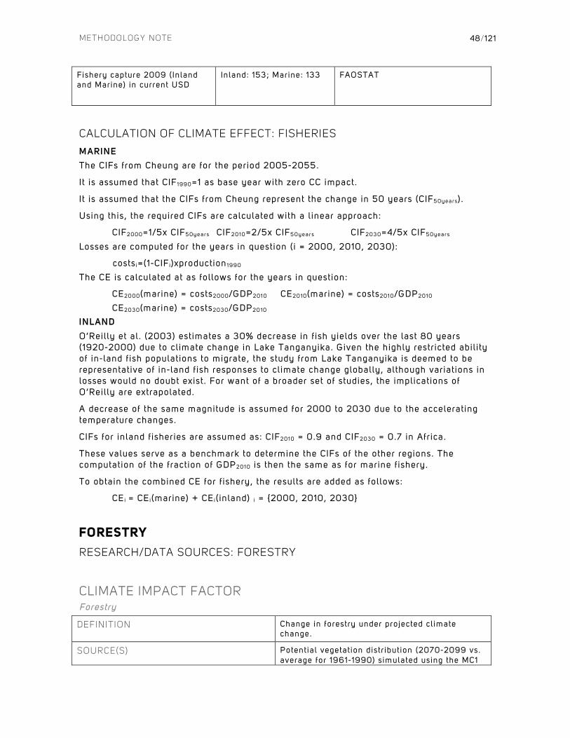
METHODOLOGY NOTE

48/121

Fishery capture 2009 ( Inland and Marine) in current USD

Inland: 153; Marine: 133 FAOSTAT

CALCULATION OF CLIMATE EFFECT: FISHERIES

MARINE The CIFs from Cheung are for the period 2005-2055.

It is assumed that CIF1990=1 as base year with zero CC impact.

I t is assumed that the CIFs from Cheung represent the change in 50 years (CIF50yea rs) .

Using this, the required CIFs are calculated with a l inear approach:

CIF2000=1/5x CIF50years CIF2010=2/5x CIF50years CIF2030=4/5x CIF50years

Losses are computed for the years in question (i = 2000, 2010, 2030):

costs i=(1-CIFi)xproduction1990

The CE is calculated at as follows for the years in question:

CE2000(marine) = costs2000/GDP2010 CE2010(marine) = costs2010/GDP2010

CE2030(marine) = costs2030/GDP2010

INLAND

O’Reilly et al. (2003) estimates a 30% decrease in f ish yields over the last 80 years (1920-2000) due to climate change in Lake Tanganyika. Given the highly restricted abil i ty of in-land fish populations to migrate, the study from Lake Tanganyika is deemed to be representative of in-land fish responses to climate change globally, although variations in losses would no doubt exist. For want of a broader set of studies, the implications of O’Reilly are extrapolated.

A decrease of the same magnitude is assumed for 2000 to 2030 due to the accelerating temperature changes.

CIFs for inland fisheries are assumed as: CIF2010 = 0.9 and CIF2030 = 0.7 in Africa.

These values serve as a benchmark to determine the CIFs of the other regions. The computation of the fraction of GDP2010 is then the same as for marine fishery.

To obtain the combined CE for f ishery, the results are added as follows:

CEi = CEi(marine) + CEi( inland) i = {2000, 2010, 2030}

FORESTRY

RESEARCH/DATA SOURCES: FORESTRY

CLIMATE IMPACT FACTOR Forestry

DEFINITION Change in forestry under projected cl imate change.

SOURCE(S) Potential vegetat ion distr ibution (2070-2099 vs. average for 1961-1990) simulated using the MC1

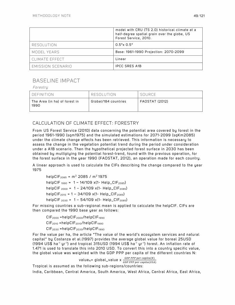
METHODOLOGY NOTE

49/121

model with CRU (TS 2.0) historical cl imate at a half-degree spatial grain over the globe, US Forest Service, 2010.

RESOLUTION 0.5°x 0.5°

MODEL YEARS Base: 1961-1990 Project ion: 2070-2099

CLIMATE EFFECT Linear


BASELINE IMPACT Forestry


The Area ( in ha) of forest in 1990

Global/184 countr ies FAOSTAT (2012)

CALCULATION OF CLIMATE EFFECT: FORESTRY

From US Forest Service (2010) data concerning the potential area covered by forest in the period 1961-1990 (sqm1975) and the simulated estimations for 2071-2099 (sqKm2085) under the climate change effects has been retrieved. This information is necessary to assess the change in the vegetation potential trend during the period under consideration under a A1B scenario. Then the hypothetical projected forest surface in 2030 has been obtained by multiplying the potential forest-trend, found with the previous operation, for the forest surface in the year 1990 (FAOSTAT, 2012), an operation made for each country.

A l inear approach is used to calculate the CIFs describing the change compared to the year 1975

helpCIF2085 = m2 2085 / m2 1975

helpCIF 1990 = 1 – 14/109 x(1- Help_CIF2085) helpCIF 2000 = 1 – 24/109 x(1- Help_CIF2085)

helpCIF2010 = 1 – 34/109 x(1- Help_CIF2085) helpCIF 2030 = 1 – 54/109 x(1- Help_CIF2085)

For missing countries a sub-regional mean is applied to calculate the helpCIF. CIFs are then compared the 1990 base year as follows:

CIF2000 =helpCIF2000/helpCIF1990



For the value per ha, the article “The value of the world’s ecosystem services and natural capital” by Costanza et al.(1997) provides the average global value for boreal 25USD (1994 US$ ha-1 yr- 1 ) and tropical 315USD (1994 US$ ha-1 yr- 1 ) forest. An inflation rate of 1.471 is used to translate this into 2010 USD. To convert this into a country specif ic value, the global value was weighted with the GDP PPP per capita of the different countries N:

valueN= global_value x !"# !!! !"# !"#$%"(!)!"# !!! !"# !"#$%"(!"#)

Tropical is assumed as the following sub-regions/countries: India, Caribbean, Central America, South America, West Africa, Central Africa, East Africa,

METHODOLOGY NOTE

50/121

South East Asia. Forest area is calculated for in the years 2000, 2010 and 2030 (in ha) as follows:

forest2000= CIF2000 x forest1990

forest2010= CIF2010 x forest1990 forest2030= CIF2030 x forest1990

And the costs of forest-change due to climate change compared to 1990:

costs2000= (forest2000 - forest1990)x valueN

costs2010= (forest2010 - forest1990)x valueN

costs2030=(forest2030 - forest1990)x valueN

The following then yields the CE for the years in question:

CE2000 = costs 2000/GDP2010

CE2010 = costs 2010/GDP2010 CE2030 = costs 2030/GDP2010

HYDRO ENERGY

RESEARCH/DATA SOURCES: HYDRO ENERGY

CLIMATE IMPACT FACTOR Hydro Energy

DEFINITION Change in developed hydropower potential due to impact of cl imate change on r iver discharge

SOURCE(S) Impact of Cl imate Change on River Discharge Projected by Mult imodel Ensemble, Nohara et al . , 2006.

Europe’s Hydropower Potential Today and in the Future, Lehner et al . , 2001

RESOLUTION 141 countr ies: 78 drawn from Nohara et al . , 36 from Lehner et al .

MODEL YEARS Nohara et al . : Base – 1990 (1981-2000), Project ion – 2090; Lehner et al . : Base – 1975 (1961-1990), Project ion – 2020 & 2070

CLIMATE EFFECT Nohara et al . : l inear; Lehner et al . : polynomial degree 2


BASELINE IMPACT Hydro Energy


Electr ic i ty production from hydroelectr ic sources in kWh

115 countr ies Lehner et al . , 2001

METHODOLOGY NOTE

51/121

for the year 2000 International Energy Agency (year)

CALCULATION OF CLIMATE EFFECT: HYDRO ENERGY

EUROPE (36 countries) Lehner et al. (2001) provides the change in developed hydropower potential (%) for the HADCM3 scenario in the years 2020 and 2070 (CIF2020, CIF2070). These values are changes compared to the base year 1975 (1961-1990). For 1975, a CIF1975 = 1 is assumed.

A polynomial of degree 2 is used to calculate helpCIF1990, helpCIF2000, helpCIF2010, helpCIF2030, describing the change compared to the year 1975.

Then the CIFs are compared to the base year 1990:

CIF2000 =helpCIF2000/helpCIF1990 CIF2010 =helpCIF2010/helpCIF1990


Hydroelectric electricity production for the required years is calculated as follows:

kWh1990= help_CIF1990 * kWh1975 = help_CIF1990 * kWh2000 /help_CIF2000

kWh2000 given by webpage kWh2010= CIF2010*kWh1990

kWh2030= CIF2030*kWh1990

Then the production changes for the years 2000, 2010 and 2030 are calculated and compared to the base year 1990 in kWh:

change2000 = kWh2000 – kWh1990 change2010 = kWh2010 – kWh1990

change2030 = kWh2030 – kWh1990

OUTSIDE EUROPE (78 countries) Nohara et al. (2006) provides river discharge data that proxies for hydro energy production potential change. Nohara provides a CIF for the year 2090 compared to the year 1990 (1981-2000).

A l inear approach is used to evaluate the CIFs for the years of interest (2000, 2010 and 2030) since only one projection year is available. The electricity production for the required years is calculated as follows:

kWh1990 = kWh2000/CIF2000

kWh2000 given from the International Energy Agency kWh2010 = CIF2010xkWh1990

kWh2030 = CIF2030xkWh1990

Production changes for the years 2000, 2010 and 2030 are then calculated and compared to the base year of 1990 in kWh as follows:

change2000 = kWh2000 – kWh1990 change2010 = kWh2010 – kWh1990

change2030 = kWh2030 – kWh1990

ECONOMIC CALCULATION

0.04 USD as price per kWh of hydropower is assumed (Europe´s Energy Portal) as a global constant. That price is multiplied by the production changes in 2000, 2010 and 2030 to obtain the losses per country as follows:

Loss2000 = 0.04 x change2000

METHODOLOGY NOTE

52/121

Loss2010 = 0.04 x change2010 Loss2030 = 0.04 x change2030

The CE is then calculated for the years in question as follows:

CE2000 = Loss2000/GDP2010 CE2010 = Loss2010/GDP2010

CE2030 = Loss2030/GDP2010

TOURISM

RESEARCH/DATA SOURCES: TOURISM

The Tourism indicator measures losses to the tourism sector globally based on modeled losses incurred through two separate effects: 1) the loss of revenues due to shorter/less advantageous winter sports seasons; and 2) the loss of revenues associated with reef-based tourism where these are under stress. An overarching assumption has been made that Tourism will have no net posit ive or negative outcome due to climate change, and will only redistribute any gains and losses. Net loss redistributions methods are detailed below.

CLIMATE IMPACT FACTOR Tourism - Winter

DEFINITION Decrease in winter tourism revenue due to cl imate change

SOURCE(S) The impact of snow scarcity on ski tourism, Steiger, 2011.


MODEL YEARS Base: 2006-2007; Project ion: 2060

MODEL DISTRIBUTION 2000 with a polynomial degree 2


Tourism – Reef-based

DEFINITION Decrease in reef tourism revenue due to cl imate change

SOURCE(S) ECLAC 2011 Barbados; WRI GIS “Reefs at Risk”, 2012


MODEL YEARS Base: 2005; Project ion: 2010-2050



BASELINE IMPACT Tourism - Winter

METHODOLOGY NOTE

53/121


Value of skier vis i ts 32 countr ies 2011 international paper on mountain tourism, Vanat, 2011.

Socioeconomic losses across affected countr ies, al l else equal, are assumed to be directly proport ional to GDP per capita. To obtain a country specif ic est imate of daily expenses GDP per capita of Country i is divided by GDP per capita in Austr ia and that rat io is then mult ipl ied by 137 euro = 181.8 USD- which is the average per day expenses for a skier vis i tor, Steiger (2011) .

The average daily expenses is mult ipl ied by the number of skier vis i ts (SV) in each country and converted into USD to obtain an overall est imate of revenue generated by winter tourists.

Tourism – Reef-based


Revenue of the tourism sector per country (2010 and forecasts unti l 2021)*

44 countr ies World Travel and Tourism Council (WTTC), 2012

*Reef tourism is est imated at 25% of the tourism sector for small is lands (based on ECLAC report (2011) ; 10% for medium-sized tropical countr ies and 5% for larger countr ies. For countr ies not included in the database (e.g. small is lands) the mean (( tourism revenue)/(GDP 2010)) per sub-region is mult ipl ied by the GDP of the missing country.

CALCULATION OF CLIMATE EFFECT: TOURISM

WINTER

The impact estimate for Tyrol in Steiger (2011) is used as a benchmark to calculate CIFs for all 33 countries with functioning ski resorts.

Steiger (2011) estimates an economic loss in the year 2060 equal to 3% of revenues generated by winter tourists; not including investment costs (snowmaking machines, higher alt itude lifts etc.) . Therefore the following CIFs are assumed for Austria: CIF1990 = 1; CIF2010=0.9933; CIF2030=0.98. A polynomial of degree 2 is used to calculate the CIF2000=0.997475

Estimations of the CIFs for the remaining countries are derived from elevation and latitude data that enable calculation of a factor that can then be applied to the Austrian estimates, as follows:

• Countries located above latitude 60 are assigned Austrian CIFs that are reduced by a factor 0.5.

• Calculate the ratio between the highest point in Austria and Countryi and apply that factor to the Austrian loss factor which is (1-CIF). Thus, if the highest point in Countryi is double of that in Austria, the loss_factor will be multiplied by a factor 2.

A redistribution factor based on a temperature factor has been used to redistribute the global losses using a weighted mean that include GDP 2010i and temperature of the countryi. The new value of losses is equivalent to the old value added to the global losses multiplied by the redistribution factor. Same for reef-based (see fuller explanation of assumptions for redistribution further below). The winter tourism revenue and the losses are calculated in 2000, 2010 and 2030 as follows:

winter_revenue2010 = !"# !!! !"# !"#$%"_!"#"(!)!"# !!! !"# !"#$%"_!"#"(!"#$%&')

x skier_visits x181.8

winter_revenue1990 = winter_revenue2010 / winter_CIF2010

METHODOLOGY NOTE

54/121

winter_costs2000 = winter_revenue1990 – winter_CIF2000 x winter_revenue1990

winter_costs2010 = winter_revenue1990 –winter_revenue2010

winter_costs2030 = winter_revenue1990 – winter_CIF2030 x winter_revenue1990

The CE for the years in question for winter tourism is then as follows:

winter_CE2000 = winter_costs2000/GDP2010

winter_CE2010 = winter_costs2010/GDP2010 winter_CE2030 = winter_costs2030/GDP2010

REEF BASED

The WRI GIS “Reefs at Risk” data sets are used to identify countries, where coral reefs are prevalent. I t is assumed that all coral reefs have the same socioeconomic signif icance and a simple country specif ic average of the WRI-specif ied risk categories is calculated for: Low, Medium, High and Very High.

The present value loss f igure is used for the A2 scenario in ECLAC Barbados (2011) that reflects the economic loss in the tourism industry due to coral reef degradation.

Furthermore, it is assumed that the cumulative loss of 1.333 bill ion USD by 2050 is distributed l inearly across the period from 2010 to 2050, which results in a 2050 loss of approximately 66.65 mill ion measured in present value USD. The period under review is transposed from 2010-2050 to 1990-2030 assuming the same results, i .e. a loss in 2030 of approximately 66.65 mill ion USD, since the effect is understood to be l inear.

The GDP growth factor is used to calculate the tourism revenue for 2030 with the WTTC data per country. Then the Barbados CIF is calculated as follows:

CIF2030(Barbados) = 1 - 66.65/(0.25 x tourism_revenue2030) = 0.67 CIF2010 = 1 - 2/4 x (1-CIF2030)=0.84

CIF2000 = 1- ¼ x (1-CIF2030)=0.92

Barbados is used as a benchmark CIF to which is added 0.01, 0.02 or 0.05 depending on the WRI category and year, see “Reef Risk” table below. By way of example, if Barbados is in the Very High category and Australia is in the LOW , Australia will have a CIF equal to 0.82.

REEF RISK

RISK CATEGORY 2000 2010 2030

LOW 0.948454 0.896907 0.823815

MEDIUM 0.938454 0.876907 0.773815

HIGH 0.928454 0.856907 0.723815

VERY HIGH 0.918454 0.836907 0.673815

The coral reef tourism revenue and the losses in 2000, 2010 and 2030 for all countries are calculated as follows:

reef_revenue2010 = tourism_revenue2010 x market_share reef_revenue1990 = Reef_revenue2010 / reef_CIF2010

reef_costs2000 = Reef_revenue1990 – reef_CIF2000 x Reef_revenue1990

reef_costs2010 = Reef_revenue1990 – reef_revenue2010

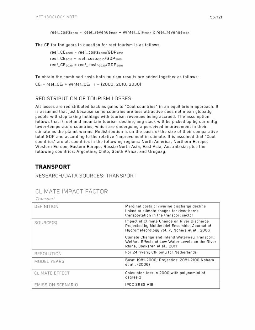
METHODOLOGY NOTE

55/121

reef_costs2030 = Reef_revenue1990 – winter_CIF2030 x reef_revenue1990

The CE for the years in question for reef tourism is as follows:

reef_CE2000 = reef_costs2000/GDP2010 reef_CE2010 = reef_costs2010/GDP2010

reef_CE2030 = reef_costs2030/GDP2010

To obtain the combined costs both tourism results are added together as follows:

CEi = reef_CEi + winter_CEi i = {2000, 2010, 2030}

REDISTRIBUTION OF TOURISM LOSSES

All losses are redistributed back as gains to "Cool countries” in an equil ibrium approach. It is assumed that just because some countries are less attractive does not mean globally people will stop taking holidays with tourism revenues being accrued. The assumption follows that if reef and mountain tourism decline, any slack will be picked up by currently lower-temperature countries, which are undergoing a perceived improvement in their climate as the planet warms. Redistribution is on the basis of the size of their comparative total GDP and according to the relative "improvement in climate. It is assumed that "Cool countries" are all countries in the following regions: North America, Northern Europe, Western Europe, Eastern Europe, Russia/North Asia, East Asia, Australasia; plus the following countries: Argentina, Chile, South Africa, and Uruguay.

TRANSPORT

RESEARCH/DATA SOURCES: TRANSPORT

CLIMATE IMPACT FACTOR Transport

DEFINITION Marginal costs of r iverine discharge decl ine l inked to cl imate chagne for r iver-borne transportat ion in the transport sector

SOURCE(S) Impact of Cl imate Change on River Discharge Projected by Mult imodel Ensemble, Journal of Hydrometeorology vol. 7, Nohara et al . , 2006

Climate Change and Inland Waterway Transport : Welfare Effects of Low Water Levels on the River Rhine, Jonkeren et al . , 2011

RESOLUTION For 24 r ivers; CIF only for Netherlands

MODEL YEARS Base: 1981-2000; Project ios: 2081-2100 Nohara et al . , (2006)

CLIMATE EFFECT Calculated loss in 2000 with polynomial of degree 2


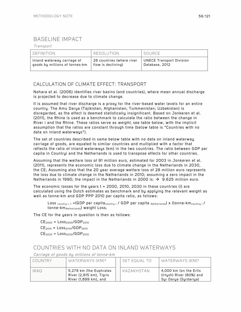
METHODOLOGY NOTE

56/121

BASELINE IMPACT Transport


Inland waterway carr iage of goods by mil l ions of tonnes-km

28 countr ies (where r iver f low is decl ining)

UNECE Transport Divis ion Database, 2012

CALCULATION OF CLIMATE EFFECT: TRANSPORT

Nohara et al. (2006) identif ies river basins (and countries), where mean annual discharge is projected to decrease due to climate change.

It is assumed that river discharge is a proxy for the river-based water levels for an entire country. The Amu Darya (Tajikistan; Afghanistan; Turkmenistan; Uzbekistan) is disregarded, as the effect is deemed statistically insignif icant. Based on Jonkeren et al. (2011), the Rhine is used as a benchmark to calculate the ratio between the change in River i and the Rhine. These ratios serve as weight , see table below, with the implicit assumption that the ratios are constant through time (below table is “Countries with no data on inland waterways”).

The set of countries described in same below table with no data on inland waterway carriage of goods, are equated to similar countries and multiplied with a factor that reflects the ratio of inland waterways (km) in the two countries. The ratio between GDP per capita in Countryi and the Netherlands is used to transpose effects for other countries.

Assuming that the welfare loss of 91 mill ion euro, estimated for 2003 in Jonkeren et al. (2011), represents the economic loss due to climate change in the Netherlands in 2030, the CE; Assuming also that the 20 year average welfare loss of 28 mill ion euro represents the loss due to climate change in the Netherlands in 2010; assuming a zero impact in the Netherlands in 1990; the impact in the Netherlands in 2000 is: à 9.625 mill ion euro.

The economic losses for the years t = 2000, 2010, 2030 in these countries ( i ) are calculated using the Dutch estimates as benchmark and by applying the relevant weight as well as tonne-km and GDP PPP 2010 per capita ratio, as follows:

Loss coun t ry i , t =(GDP per capitacoun t ry i / GDP per capita Ne the r l ands) x (tonne-kmcoun t ry i / tonne-kmNethe r lands) weight Losst

The CE for the years in question is then as follows:

CE2000 = Loss2000/GDP2010

CE2010 = Loss2010/GDP2010 CE2030 = Loss2030/GDP2010

COUNTRIES WITH NO DATA ON INLAND WATERWAYS Carr iage of goods by mil l ions of tonne-km

COUNTRY WATERWAYS (KM)* SET EQUAL TO WATERWAYS (KM)*

IRAQ 5,279 km (the Euphrates River (2,815 km), Tigr is River (1 ,899 km), and

KAZAKHSTAN 4,000 km (on the Ert is ( I r tysh) River (80%) and Syr Darya (Syrdariya)

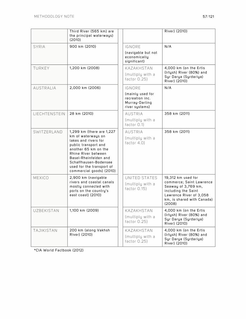
METHODOLOGY NOTE

57/121

Third River (565 km) are the principal waterways) (2010)

River) (2010)

SYRIA 900 km (2010) IGNORE

(navigable but not economically signif icant)

N/A

TURKEY 1 ,200 km (2008) KAZAKHSTAN

(multiply with a factor 0.25)

4,000 km (on the Ert is ( I r tysh) River (80%) and Syr Darya (Syrdariya) River) (2010)

AUSTRALIA 2,000 km (2006) IGNORE

(mainly used for recreation inc. Murray-Darl ing r iver systems)

N/A

LIECHTENSTEIN 28 km (2010) AUSTRIA


358 km (2011)

SWITZERLAND 1 ,299 km (there are 1 ,227 km of waterways on lakes and r ivers for public transport and another 65 km on the Rhine River between Basel-Rheinfelden and Schaffhausen-Bodensee used for the transport of commercial goods) (2010)

AUSTRIA


358 km (2011)

MEXICO 2,900 km (navigable r ivers and coastal canals mostly connected with ports on the country's east coast) (2010)

UNITED STATES


19,312 km used for commerce; Saint Lawrence Seaway of 3,769 km, including the Saint Lawrence River of 3,058 km, is shared with Canada) (2008)

UZBEKISTAN 1 ,100 km (2009) KAZAKHSTAN



TAJIKISTAN 200 km (along Vakhsh River) (2010)

KAZAKHSTAN



*CIA World Factbook (2012)

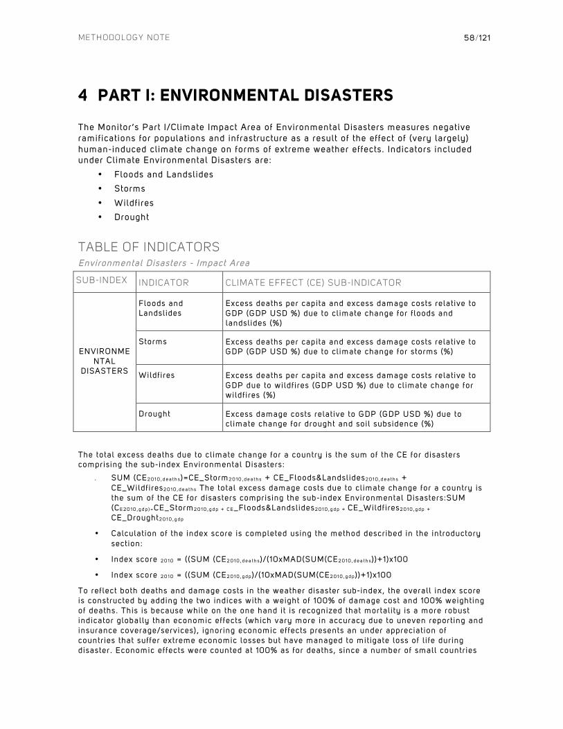
METHODOLOGY NOTE

58/121

4 PART I: ENVIRONMENTAL DISASTERS

The Monitor’s Part I/Climate Impact Area of Environmental Disasters measures negative ramifications for populations and infrastructure as a result of the effect of (very largely) human-induced climate change on forms of extreme weather effects. Indicators included under Climate Environmental Disasters are:

• Floods and Landslides

• Storms

• Wildfires

• Drought

TABLE OF INDICATORS Environmental Disasters - Impact Area

SUB-INDEX INDICATOR CLIMATE EFFECT (CE) SUB-INDICATOR

ENVIRONMENTAL

DISASTERS

Floods and Landsl ides

Excess deaths per capita and excess damage costs relat ive to GDP (GDP USD %) due to cl imate change for f loods and landsl ides (%)

Storms Excess deaths per capita and excess damage costs relat ive to GDP (GDP USD %) due to cl imate change for storms (%)

Wildf ires Excess deaths per capita and excess damage costs relat ive to GDP due to wildf ires (GDP USD %) due to cl imate change for wildf ires (%)

Drought Excess damage costs relat ive to GDP (GDP USD %) due to cl imate change for drought and soil subsidence (%)

The total excess deaths due to cl imate change for a country is the sum of the CE for disasters comprising the sub-index Environmental Disasters:

• SUM (CE2 0 1 0 , d e a t h s )=CE_Storm2 0 1 0 , d e a t h s + CE_Floods&Landslides2 0 1 0 , d e a t h s + CE_Wildf ires2 0 1 0 , d e a t h s The total excess damage costs due to cl imate change for a country is the sum of the CE for disasters comprising the sub-index Environmental Disasters:SUM (CE 2 0 1 0 , g d p ) =CE_Storm2 0 1 0 , g d p + C E_Floods&Landslides2 0 1 0 , g d p + CE_Wildf ires2 0 1 0 , g d p +

CE_Drought2 0 1 0 , g d p

• Calculat ion of the index score is completed using the method described in the introductory section:

• Index score 2 0 1 0 = ( (SUM (CE2 0 1 0 , d e a t h s )/ (10xMAD(SUM(CE2 0 1 0 , d e a t h s ) )+1)x100

• Index score 2 0 1 0 = ( (SUM (CE2 0 1 0 , g d p )/(10xMAD(SUM(CE2 0 1 0 , g d p ) )+1)x100

To reflect both deaths and damage costs in the weather disaster sub-index, the overall index score is constructed by adding the two indices with a weight of 100% of damage cost and 100% weighting of deaths. This is because while on the one hand i t is recognized that mortal i ty is a more robust indicator globally than economic effects (which vary more in accuracy due to uneven report ing and insurance coverage/services), ignoring economic effects presents an under appreciat ion of countr ies that suffer extreme economic losses but have managed to mit igate loss of l i fe during disaster. Economic effects were counted at 100% as for deaths, s ince a number of small countr ies

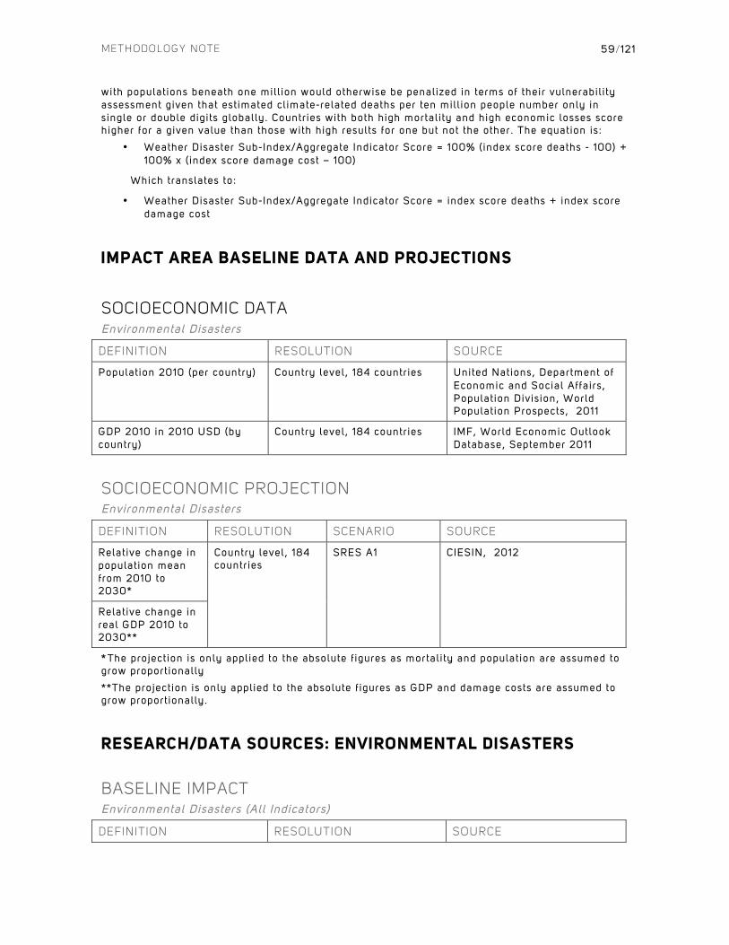
METHODOLOGY NOTE

59/121

with populat ions beneath one mil l ion would otherwise be penalized in terms of their vulnerabil i ty assessment given that est imated cl imate-related deaths per ten mil l ion people number only in single or double digits globally. Countr ies with both high mortal i ty and high economic losses score higher for a given value than those with high results for one but not the other. The equation is :

• Weather Disaster Sub-Index/Aggregate Indicator Score = 100% (index score deaths - 100) + 100% x ( index score damage cost – 100)

Which translates to:

• Weather Disaster Sub-Index/Aggregate Indicator Score = index score deaths + index score damage cost


SOCIOECONOMIC DATA Environmental Disasters


Population 2010 (per country) Country level, 184 countr ies United Nations, Department of Economic and Social Affairs, Populat ion Division, World Populat ion Prospects, 2011


Country level, 184 countr ies IMF, World Economic Outlook Database, September 2011

SOCIOECONOMIC PROJECTION Environmental Disasters


Relative change in populat ion mean from 2010 to 2030*


SRES A1 CIESIN, 2012

Relat ive change in real GDP 2010 to 2030**

* The project ion is only applied to the absolute f igures as mortal i ty and populat ion are assumed to grow proport ionally

**The project ion is only applied to the absolute f igures as GDP and damage costs are assumed to grow proport ionally.

RESEARCH/DATA SOURCES: ENVIRONMENTAL DISASTERS

BASELINE IMPACT Environmental Disasters (All Indicators)


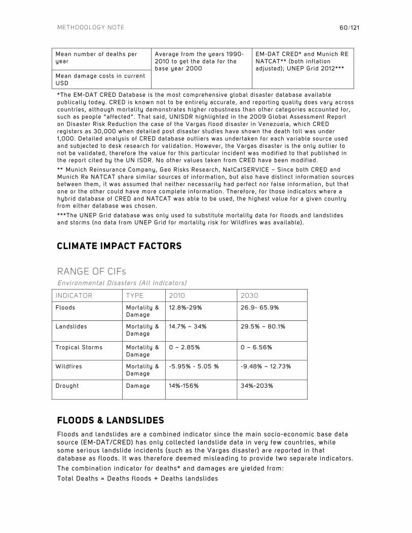
METHODOLOGY NOTE

60/121

Mean number of deaths per year

Average from the years 1990-2010 to get the data for the base year 2000

EM-DAT CRED* and Munich RE NATCAT** (both inflat ion adjusted); UNEP Grid 2012***

Mean damage costs in current USD

*The EM-DAT CRED Database is the most comprehensive global disaster database available publically today. CRED is known not to be entirely accurate, and report ing quali ty does vary across countr ies, although mortal i ty demonstrates higher robustness than other categories accounted for, such as people “affected”. That said, UNISDR highlighted in the 2009 Global Assessment Report on Disaster Risk Reduction the case of the Vargas f lood disaster in Venezuela, which CRED registers as 30,000 when detailed post disaster studies have shown the death tol l was under 1 ,000. Detailed analysis of CRED database outl iers was undertaken for each variable source used and subjected to desk research for val idation. However, the Vargas disaster is the only outl ier to not be val idated, therefore the value for this part icular incident was modif ied to that published in the report ci ted by the UN ISDR. No other values taken from CRED have been modif ied.

** Munich Reinsurance Company, Geo Risks Research, NatCatSERVICE – Since both CRED and Munich Re NATCAT share similar sources of information, but also have dist inct information sources between them, i t was assumed that neither necessari ly had perfect nor false information, but that one or the other could have more complete information. Therefore, for those indicators where a hybrid database of CRED and NATCAT was able to be used, the highest value for a given country from either database was chosen.

***The UNEP Grid database was only used to substi tute mortal i ty data for f loods and landsl ides and storms (no data from UNEP Grid for mortal i ty r isk for Wildf ires was available) .


RANGE OF CIFs Environmental Disasters (All Indicators)

INDICATOR TYPE 2010 2030

Floods Mortal i ty & Damage

12.8%-29% 26.9- 65.9%

Landsl ides Mortal i ty & Damage

14.7% – 34%

29.5% – 80.1%

Tropical Storms Mortal i ty & Damage

0 – 2.85% 0 – 6.56%

Wildf ires Mortal i ty & Damage

-5.95% - 5.05 % -9.48% – 12.73%

Drought Damage 14%-156% 34%-203%

FLOODS & LANDSLIDES

Floods and landslides are a combined indicator since the main socio-economic base data source (EM-DAT/CRED) has only collected landslide data in very few countries, while some serious landslide incidents (such as the Vargas disaster) are reported in that database as floods. It was therefore deemed misleading to provide two separate indicators. The combination indicator for deaths* and damages are yielded from:

Total Deaths = Deaths floods + Deaths landslides

METHODOLOGY NOTE

61/121

Total Damages = Damages floods + Damages landslides

RESEARCH SOURCES: FLOODS & LANDSLIDES

CLIMATE DATA Floods

DEFINITION Effect of change in magnitude and frequency of extreme precipitat ion with return t ime of 20 years accumulated in 24 hours due to cl imate change on f lood mortal i ty and economic damages

SOURCE(S) Changes in Temperature and Precipitat ion Extremes in the IPCC Ensemble of Global Coupled Model Simulations, Kharin et al . , 2007.

The Death Toll From Natural Disasters: The Role of Income, Geography, and Inst i tut ions, Kahn, 2005

Impact Of Cl imate Change On Snowmelt Runoff :

A Case Study Of Tamakoshi Basin In Nepal, Shilpakar et al . , 2011.

RESOLUTION Sub continental scale, 9 sub regions


MODEL YEARS Base: 1981-2000; Project ion: 2046-2065, 2081-2100

MODEL DISTRIBUTION Exponential

UNIT OF MEASUREMENT Increase factor for number of deaths and damages associated with f loods due to cl imate change.

DYNAMIC ADJUSTMENT Base year: CIF=1; R was used to f ind the best f i t exponential function for these three points. With this polynomial the CIFs were calculated for 2010 and 2030. Two dif ferent CIFs were obtained, one for deaths and the other for damages, as the effect of f loods on each indicator is dif ferent.

CLIMATE EFFECT CE_deaths_per_capita(year)=CIF(year)*UNEPGrid_mortal i ty/populat ion(2010)

CE_costs_per_GDP(year)=CIF(year)*Max{MunichRe_costs;CRED_costs1990-2010}/GDP(2010)

Year = 2000, 2010, 2030

OUTPUT Excess deaths due to cl imate change for f loods in total and as a share of populat ion.

Damage costs due to cl imate change for f loods in total and as a share of populat ion.

Landslides

DEFINITION Effect of change in magnitude and frequency of extreme precipitat ion with return t ime of 20 years accumulated in 24 hours due to cl imate change on landsl ide mortal i ty and economic damages

SOURCE(S) Changes in Temperature and Precipitat ion Extremes in the IPCC Ensemble of Global Coupled Model Simulations, Kharin et al . ,

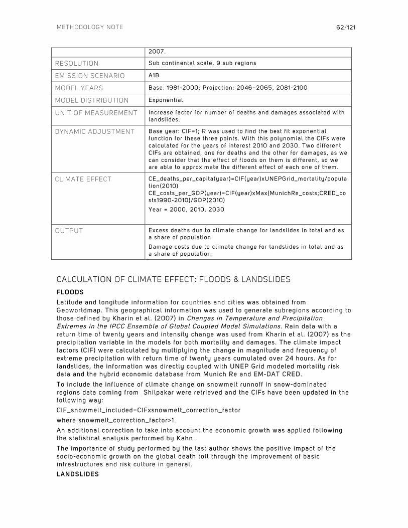
METHODOLOGY NOTE

62/121

2007.

RESOLUTION Sub continental scale, 9 sub regions


MODEL YEARS Base: 1981-2000; Project ion: 2046–2065, 2081-2100

MODEL DISTRIBUTION Exponential

UNIT OF MEASUREMENT Increase factor for number of deaths and damages associated with landsl ides.

DYNAMIC ADJUSTMENT Base year: CIF=1; R was used to f ind the best f i t exponential function for these three points. With this polynomial the CIFs were calculated for the years of interest 2010 and 2030. Two dif ferent CIFs are obtained, one for deaths and the other for damages, as we can consider that the effect of f loods on them is dif ferent, so we are able to approximate the dif ferent effect of each one of them.

CLIMATE EFFECT CE_deaths_per_capita(year)=CIF(year)xUNEPGrid_mortal i ty/populat ion(2010) CE_costs_per_GDP(year)=CIF(year)xMax{MunichRe_costs;CRED_costs1990-2010}/GDP(2010)

Year = 2000, 2010, 2030

OUTPUT Excess deaths due to cl imate change for landsl ides in total and as a share of populat ion.

Damage costs due to cl imate change for landsl ides in total and as a share of populat ion.

CALCULATION OF CLIMATE EFFECT: FLOODS & LANDSLIDES

FLOODS Latitude and longitude information for countries and cit ies was obtained from Geoworldmap. This geographical information was used to generate subregions according to those defined by Kharin et al. (2007) in Changes in Temperature and Precipitation Extremes in the IPCC Ensemble of Global Coupled Model Simulations . Rain data with a return time of twenty years and intensity change was used from Kharin et al. (2007) as the precipitation variable in the models for both mortality and damages. The climate impact factors (CIF) were calculated by multiplying the change in magnitude and frequency of extreme precipitation with return time of twenty years cumulated over 24 hours. As for landslides, the information was directly coupled with UNEP Grid modeled mortality risk data and the hybrid economic database from Munich Re and EM-DAT CRED.

To include the influence of climate change on snowmelt runnoff in snow-dominated regions data coming from Shilpakar were retrieved and the CIFs have been updated in the following way: CIF_snowmelt_included=CIFxsnowmelt_correction_factor

where snowmelt_correction_factor>1.

An additional correction to take into account the economic growth was applied following the statistical analysis performed by Kahn.

The importance of study performed by the last author shows the posit ive impact of the socio-economic growth on the global death toll through the improvement of basic infrastructures and risk culture in general. LANDSLIDES

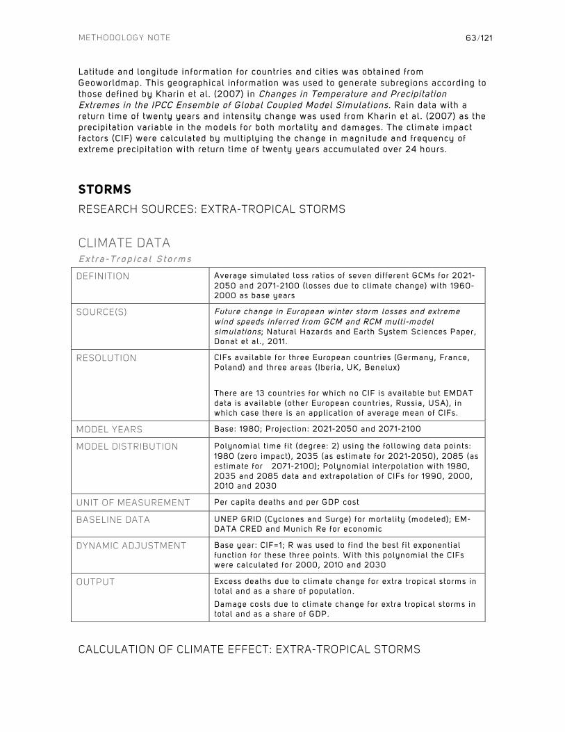
METHODOLOGY NOTE

63/121

Latitude and longitude information for countries and cit ies was obtained from Geoworldmap. This geographical information was used to generate subregions according to those defined by Kharin et al. (2007) in Changes in Temperature and Precipitation Extremes in the IPCC Ensemble of Global Coupled Model Simulations . Rain data with a return time of twenty years and intensity change was used from Kharin et al. (2007) as the precipitation variable in the models for both mortality and damages. The climate impact factors (CIF) were calculated by multiplying the change in magnitude and frequency of extreme precipitation with return time of twenty years accumulated over 24 hours.

STORMS

RESEARCH SOURCES: EXTRA-TROPICAL STORMS

CLIMATE DATA E x t r a - T r o p i c a l S t o r m s

DEFINITION Average simulated loss rat ios of seven dif ferent GCMs for 2021-2050 and 2071-2100 (losses due to cl imate change) with 1960-2000 as base years

SOURCE(S) Future change in European winter storm losses and extreme wind speeds inferred from GCM and RCM mult i-model s imulations ; Natural Hazards and Earth System Sciences Paper, Donat et al . , 2011.

RESOLUTION CIFs available for three European countr ies (Germany, France, Poland) and three areas ( Iberia, UK, Benelux)

There are 13 countr ies for which no CIF is available but EMDAT data is available (other European countr ies, Russia, USA), in which case there is an applicat ion of average mean of CIFs.

MODEL YEARS Base: 1980; Project ion: 2021-2050 and 2071-2100

MODEL DISTRIBUTION Polynomial t ime f i t (degree: 2) using the following data points: 1980 (zero impact) , 2035 (as est imate for 2021-2050), 2085 (as est imate for 2071-2100); Polynomial interpolat ion with 1980, 2035 and 2085 data and extrapolat ion of CIFs for 1990, 2000, 2010 and 2030

UNIT OF MEASUREMENT Per capita deaths and per GDP cost

BASELINE DATA UNEP GRID (Cyclones and Surge) for mortal i ty (modeled); EM-DATA CRED and Munich Re for economic

DYNAMIC ADJUSTMENT Base year: CIF=1; R was used to f ind the best f i t exponential function for these three points. With this polynomial the CIFs were calculated for 2000, 2010 and 2030

OUTPUT Excess deaths due to cl imate change for extra tropical storms in total and as a share of populat ion.

Damage costs due to cl imate change for extra tropical storms in total and as a share of GDP.

CALCULATION OF CLIMATE EFFECT: EXTRA-TROPICAL STORMS

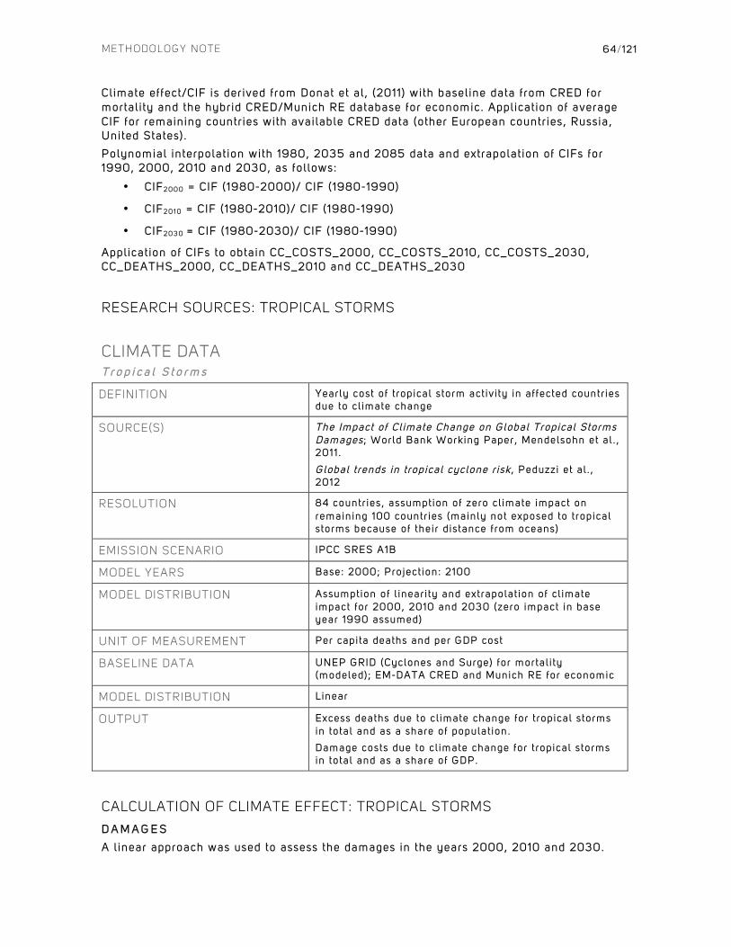
METHODOLOGY NOTE

64/121

Climate effect/CIF is derived from Donat et al, (2011) with baseline data from CRED for mortality and the hybrid CRED/Munich RE database for economic. Application of average CIF for remaining countries with available CRED data (other European countries, Russia, United States).

Polynomial interpolation with 1980, 2035 and 2085 data and extrapolation of CIFs for 1990, 2000, 2010 and 2030, as follows:

• CIF2000 = CIF (1980-2000)/ CIF (1980-1990)

• CIF2010 = CIF (1980-2010)/ CIF (1980-1990)

• CIF2030 = CIF (1980-2030)/ CIF (1980-1990)

Application of CIFs to obtain CC_COSTS_2000, CC_COSTS_2010, CC_COSTS_2030, CC_DEATHS_2000, CC_DEATHS_2010 and CC_DEATHS_2030

RESEARCH SOURCES: TROPICAL STORMS

CLIMATE DATA T r o p i c a l S t o r m s

DEFINITION Yearly cost of tropical storm activi ty in affected countr ies due to cl imate change

SOURCE(S) The Impact of Cl imate Change on Global Tropical Storms Damages ; World Bank Working Paper, Mendelsohn et al . , 2011.

Global trends in tropical cyclone r isk , Peduzzi et al . , 2012

RESOLUTION 84 countr ies, assumption of zero cl imate impact on remaining 100 countr ies (mainly not exposed to tropical storms because of their distance from oceans)



MODEL DISTRIBUTION Assumption of l ineari ty and extrapolat ion of cl imate impact for 2000, 2010 and 2030 (zero impact in base year 1990 assumed)

UNIT OF MEASUREMENT Per capita deaths and per GDP cost

BASELINE DATA UNEP GRID (Cyclones and Surge) for mortal i ty (modeled); EM-DATA CRED and Munich RE for economic


OUTPUT Excess deaths due to cl imate change for tropical storms in total and as a share of populat ion.

Damage costs due to cl imate change for tropical storms in total and as a share of GDP.

CALCULATION OF CLIMATE EFFECT: TROPICAL STORMS

D A M A G E S

A linear approach was used to assess the damages in the years 2000, 2010 and 2030.

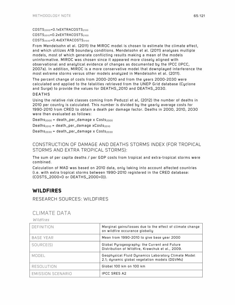
METHODOLOGY NOTE

65/121

COSTS2 0 0 0=0.1xEXTRACOSTS2 1 0 0



From Mendelsohn et al. (2011) the MIROC model is chosen to estimate the climate effect, and which util izes A1B boundary conditions. Mendelsohn et al. (2011) analyses multiple models, most of which generate conflicting results making a mean of the models uninformative. MIROC was chosen since it appeared more closely aligned with observational and analytical evidence of changes as documented by the IPCC (IPCC, 2007a). In addition, MIROC is a more conservative model that downplayed interference the most extreme storms versus other models analyzed in Mendelsohn et al. (2011).

The percent change of costs from 2000-2010 and from the years 2000-2030 were calculated and applied to the fatalit ies retrieved from the UNEP Grid database (Cyclone and Surge) to provide the values for DEATHS_2010 and DEATHS_2030. D E A T H S

Using the relative risk classes coming from Peduzzi et al, (2012) the number of deaths in 2010 per country is calculated. This number is divided by the yearly average costs for 1990-2010 from CRED to obtain a death per damage factor. Deaths in 2000, 2010, 2030 were then evaluated as follows: Deaths2000 = death_per_damage x Costs2000

Deaths2010 = death_per_damage xCosts2010

Deaths2030 = death_per_damage x Costs2030

CONSTRUCTION OF DAMAGE AND DEATHS STORMS INDEX (FOR TROPICAL STORMS AND EXTRA TROPICAL STORMS):

The sum of per capita deaths / per GDP costs from tropical and extra-tropical storms were combined.

Calculation of MAD was based on 2010 data, only taking into account affected countries ( i .e. with extra tropical storms between 1990-2010 registered in the CRED database: (COSTS_2000>0 or DEATHS_2000>0)).

WILDFIRES

RESEARCH SOURCES: WILDFIRES

CLIMATE DATA Wildfires

DEFINITION Marginal gains/losses due to the effect of cl imate change on wildf ire occurance globally

BASE YEAR Mean from 1990-2010 to give base year 2000

SOURCE(S) Global Pyrogeography: the Current and Future Distr ibution of Wildf ire, Krawchuk et al . , 2009.

MODEL Geophysical Fluid Dynamics Laboratory Cl imate Model 2.1 ; dynamic global vegetat ion models (DGVMs)

RESOLUTION Global 100 km on 100 km

EMISSION SCENARIO IPCC SRES A2

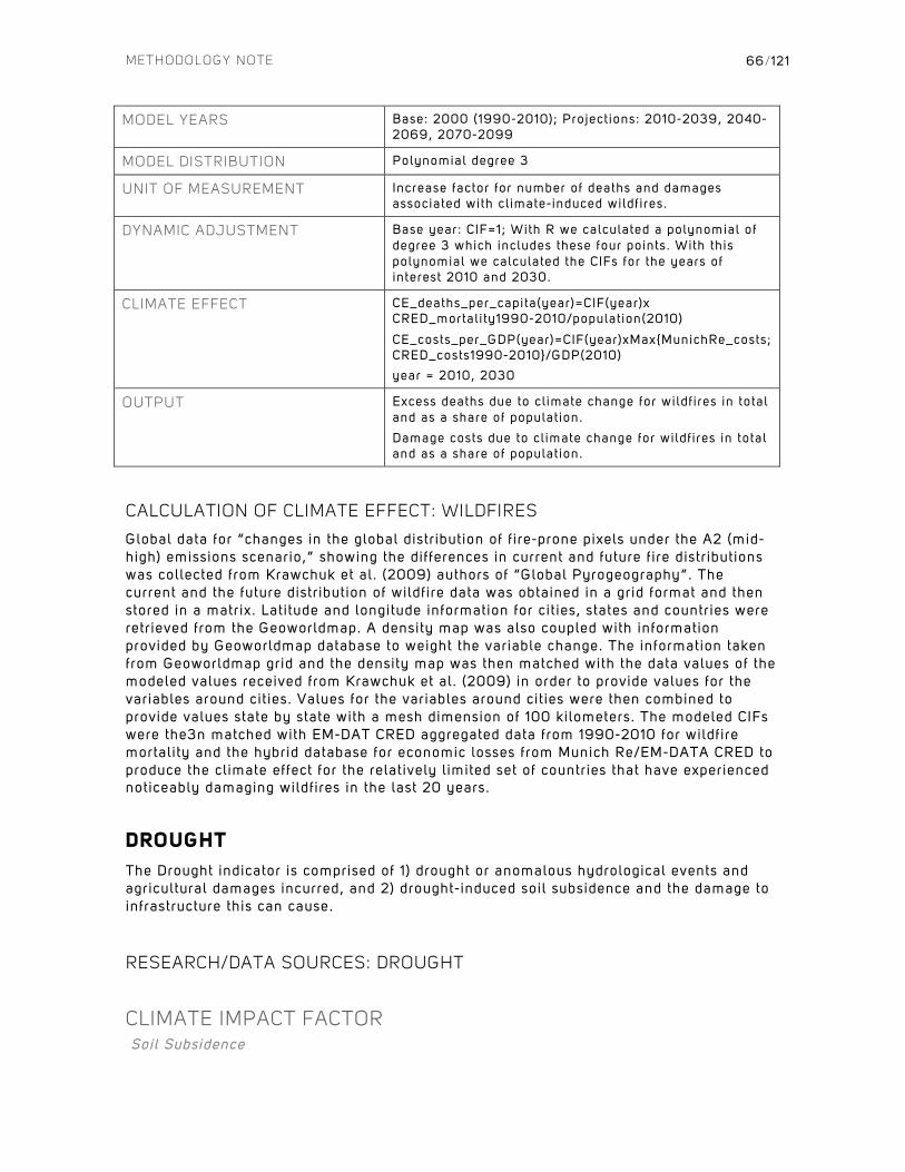
METHODOLOGY NOTE

66 /121

MODEL YEARS Base: 2000 (1990-2010); Project ions: 2010-2039, 2040-2069, 2070-2099

MODEL DISTRIBUTION Polynomial degree 3

UNIT OF MEASUREMENT Increase factor for number of deaths and damages associated with cl imate-induced wildf ires.

DYNAMIC ADJUSTMENT Base year: CIF=1; With R we calculated a polynomial of degree 3 which includes these four points. With this polynomial we calculated the CIFs for the years of interest 2010 and 2030.

CLIMATE EFFECT CE_deaths_per_capita(year)=CIF(year)x CRED_mortal i ty1990-2010/populat ion(2010)

CE_costs_per_GDP(year)=CIF(year)xMax{MunichRe_costs;CRED_costs1990-2010}/GDP(2010)

year = 2010, 2030

OUTPUT Excess deaths due to cl imate change for wildf ires in total and as a share of populat ion.

Damage costs due to cl imate change for wildf ires in total and as a share of populat ion.

CALCULATION OF CLIMATE EFFECT: WILDFIRES

Global data for “changes in the global distr ibution of f ire-prone pixels under the A2 (mid-high) emissions scenario,” showing the differences in current and future f ire distributions was collected from Krawchuk et al. (2009) authors of “Global Pyrogeography”. The current and the future distribution of wildfire data was obtained in a grid format and then stored in a matrix. Latitude and longitude information for cit ies, states and countries were retrieved from the Geoworldmap. A density map was also coupled with information provided by Geoworldmap database to weight the variable change. The information taken from Geoworldmap grid and the density map was then matched with the data values of the modeled values received from Krawchuk et al. (2009) in order to provide values for the variables around cit ies. Values for the variables around cit ies were then combined to provide values state by state with a mesh dimension of 100 kilometers. The modeled CIFs were the3n matched with EM-DAT CRED aggregated data from 1990-2010 for wildfire mortality and the hybrid database for economic losses from Munich Re/EM-DATA CRED to produce the climate effect for the relatively l imited set of countries that have experienced noticeably damaging wildfires in the last 20 years.

DROUGHT

The Drought indicator is comprised of 1) drought or anomalous hydrological events and agricultural damages incurred, and 2) drought-induced soil subsidence and the damage to infrastructure this can cause.

RESEARCH/DATA SOURCES: DROUGHT

CLIMATE IMPACT FACTOR Soil Subsidence

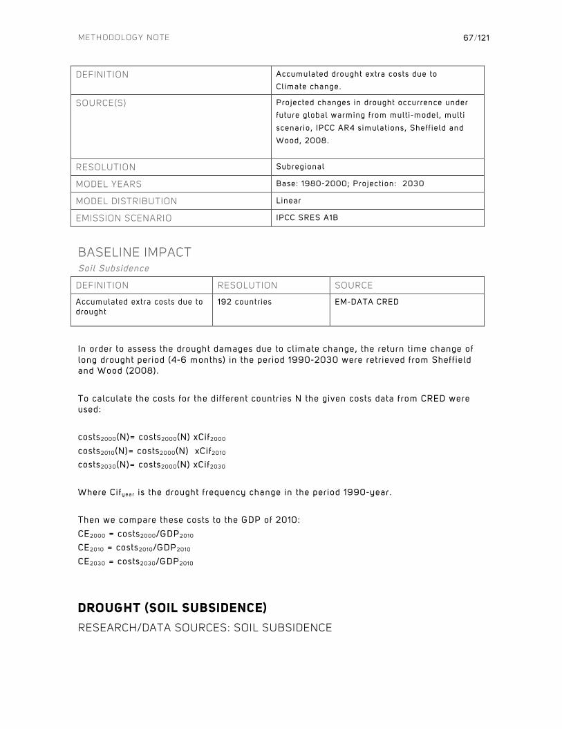
METHODOLOGY NOTE

67/121

DEFINITION Accumulated drought extra costs due to

Cl imate change.

SOURCE(S) Projected changes in drought occurrence under

future global warming from mult i-model, mult i

scenario, IPCC AR4 simulations, Sheff ield and

Wood, 2008.

RESOLUTION Subregional




BASELINE IMPACT Soil Subsidence


Accumulated extra costs due to drought

192 countr ies EM-DATA CRED

In order to assess the drought damages due to climate change, the return time change of long drought period (4-6 months) in the period 1990-2030 were retrieved from Sheffield and Wood (2008).

To calculate the costs for the different countries N the given costs data from CRED were used:

costs2000(N)= costs2000(N) xCif2000



Where Cifyea r is the drought frequency change in the period 1990-year.

Then we compare these costs to the GDP of 2010:


CE2030 = costs2030/GDP2010

DROUGHT (SOIL SUBSIDENCE)

RESEARCH/DATA SOURCES: SOIL SUBSIDENCE

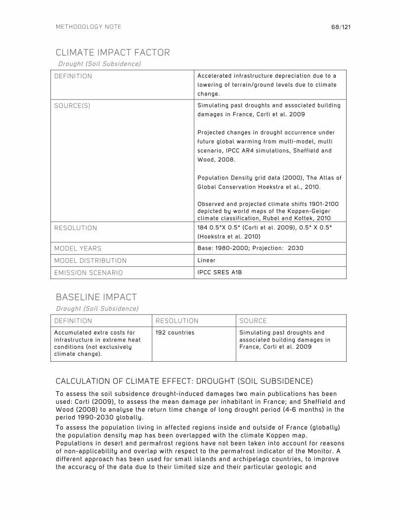
METHODOLOGY NOTE

68/121

CLIMATE IMPACT FACTOR Drought (Soil Subsidence)

DEFINITION Accelerated infrastructure depreciat ion due to a

lowering of terrain/ground levels due to cl imate

change.

SOURCE(S) Simulating past droughts and associated building

damages in France, Cort i et al . 2009

Projected changes in drought occurrence under

future global warming from mult i-model, mult i

scenario, IPCC AR4 simulations, Sheff ield and

Wood, 2008.

Populat ion Density grid data (2000), The Atlas of

Global Conservation Hoekstra et al . , 2010.

Observed and projected cl imate shif ts 1901-2100 depicted by world maps of the Koppen-Geiger cl imate classif icat ion, Rubel and Kottek, 2010

RESOLUTION 184 0.5°X 0.5° (Cort i et al . 2009), 0.5° X 0.5°

(Hoekstra et al . 2010)




BASELINE IMPACT Drought (Soil Subsidence)


Accumulated extra costs for infrastructure in extreme heat condit ions (not exclusively cl imate change).

192 countr ies Simulat ing past droughts and associated building damages in France, Cort i et al . 2009

CALCULATION OF CLIMATE EFFECT: DROUGHT (SOIL SUBSIDENCE)

To assess the soil subsidence drought-induced damages two main publications has been used: Corti (2009), to assess the mean damage per inhabitant in France; and Sheffield and Wood (2008) to analyse the return time change of long drought period (4-6 months) in the period 1990-2030 globally.

To assess the population l iving in affected regions inside and outside of France (globally) the population density map has been overlapped with the climate Koppen map. Populations in desert and permafrost regions have not been taken into account for reasons of non-applicabil ity and overlap with respect to the permafrost indicator of the Monitor. A different approach has been used for small islands and archipelago countries, to improve the accuracy of the data due to their l imited size and their particular geologic and

METHODOLOGY NOTE

69/121

infrastructural conditions. For these reasons they have the same GDP fraction as the most similar larger sub-regional country or a regional basket-country mean.

To calculate the costs for the different countries N the given costs, the affected people and the GDP PPP per capita 2010 of France were used and the number of affected people and their GDP PPP per capita 2010 of country N:

costs2000(N)= costs2000(FRA) ∗ [!""#$%#&(!)∗!"#_!!!!"#"(!)][!""#$%#&(!"#)∗!"#_!!!!"#"(!"#)]

xCif2000

costs2010(N)= costs2000(FRA) ∗ [!""#$%#&(!)∗!"#_!!!!"#"(!)][!""#$%#&(!"#)∗!"#_!!!!"#"(!"#)]

xCif2010

costs2030(N)= costs2000(FRA) ∗ [!""#$%#&(!)∗!"#_!!!!"#"(!)][!""#$%#&(!"#)∗!"#_!!!!"#"(!"#)]

xCif2030

Where Cifyea r is the drought frequency change in the period 1990-year.

Then we compare these costs to the GDP of 2010: CE2000 = costs2000/GDP2010


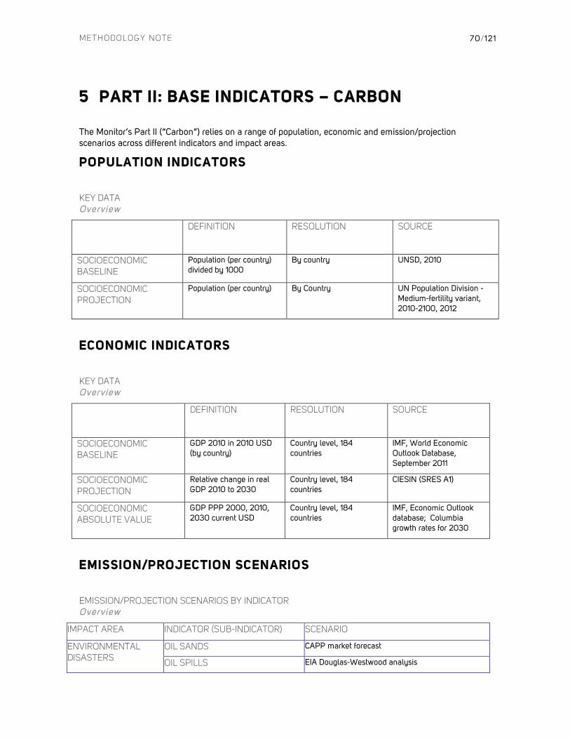
METHODOLOGY NOTE

70/121

5 PART II: BASE INDICATORS – CARBON

The Monitor’s Part II (“Carbon”) relies on a range of population, economic and emission/projection scenarios across different indicators and impact areas.

POPULATION INDICATORS

KEY DATA Overview

DEFINITION

RESOLUTION SOURCE

SOCIOECONOMIC BASELINE


By country UNSD, 2010

SOCIOECONOMIC PROJECTION

Population (per country) By Country UN Population Division - Medium-fertility variant, 2010-2100, 2012

ECONOMIC INDICATORS

KEY DATA Overview

DEFINITION

RESOLUTION SOURCE

SOCIOECONOMIC BASELINE


Country level, 184 countries

IMF, World Economic Outlook Database, September 2011

SOCIOECONOMIC PROJECTION



CIESIN (SRES A1)

SOCIOECONOMIC ABSOLUTE VALUE

GDP PPP 2000, 2010, 2030 current USD


IMF, Economic Outlook database; Columbia growth rates for 2030

EMISSION/PROJECTION SCENARIOS

EMISSION/PROJECTION SCENARIOS BY INDICATOR Overview

IMPACT AREA INDICATOR (SUB-INDICATOR) SCENARIO

ENVIRONMENTAL DISASTERS

OIL SANDS CAPP market forecast

OIL SPILLS EIA Douglas-Westwood analysis

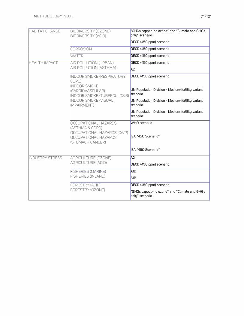
METHODOLOGY NOTE

71/121

HABITAT CHANGE BIODIVERSITY (OZONE) BIODIVERSITY (ACID)

“GHGs capped-no ozone” and “Climate and GHGs only” scenario

OECD (450 ppm) scenario

CORROSION OECD (450 ppm) scenario

WATER OECD (450 ppm) scenario

HEALTH IMPACT AIR POLLUTION (URBAN) AIR POLLUTION (ASTHMA)


A2

INDOOR SMOKE (RESPIRATORY, COPD) INDOOR SMOKE (CARDIOVASCULAR) INDOOR SMOKE (TUBERCULOSIS) INDOOR SMOKE (VISUAL IMPAIRMENT)


UN Population Division - Medium-fertility variant scenario



OCCUPATIONAL HAZARDS (ASTHMA & COPD) OCCUPATIONAL HAZARDS (CWP) OCCUPATIONAL HAZARDS (STOMACH CANCER)

WHO scenario

IEA “450 Scenario”

IEA “450 Scenario”

INDUSTRY STRESS AGRICULTURE (OZONE) AGRICULTURE (ACID)

A2


FISHERIES (MARINE) FISHERIES (INLAND)

A1B

A1B

FORESTRY (ACID) FORESTRY (OZONE)


“GHGs capped-no ozone” and “Climate and GHGs only” scenario

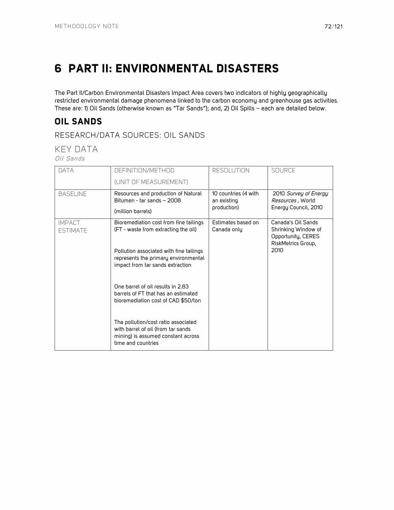
METHODOLOGY NOTE

72/121

6 PART II: ENVIRONMENTAL DISASTERS

The Part II/Carbon Environmental Disasters Impact Area covers two indicators of highly geographically restricted environmental damage phenomena linked to the carbon economy and greenhouse gas activities. These are: 1) Oil Sands (otherwise known as “Tar Sands”); and, 2) Oil Spills – each are detailed below.

OIL SANDS

RESEARCH/DATA SOURCES: OIL SANDS

KEY DATA Oil Sands

DATA DEFINITION/METHOD

(UNIT OF MEASUREMENT)

RESOLUTION SOURCE

BASELINE

Resources and production of Natural Bitumen - tar sands – 2008

(million barrels)

10 countries (4 with an existing production)

2010 Survey of Energy Resources , World Energy Council, 2010

IMPACT ESTIMATE

Bioremediation cost from fine tailings (FT - waste from extracting the oil)

Pollution associated with fine tailings represents the primary environmental impact from tar sands extraction

One barrel of oil results in 2.83 barrels of FT that has an estimated bioremediation cost of CAD $50/ton

The pollution/cost ratio associated with barrel of oil (from tar sands mining) is assumed constant across time and countries

Estimates based on Canada only

Canada’s Oil Sands Shrinking Window of Opportunity, CERES RiskMetrics Group, 2010

METHODOLOGY NOTE

73/121

IMPACT PROJECTIONS

Only Canada is assumed to have tar sands production in 2000

Canada, USA, Indonesia, and Russia have tar sand production in 2008, which is assumed to represent 2010. The 3 latter countries are assumed to have the same tar sand oil production growth as Canada.

7 other countries are assumed to have a production in 2030, based on the World Energy Council Publication, where it is assumed they have the same production/total resources ratio*

N/A CAPP Canadian Crude Oil Production Forecast 2011 – 2025, Canadian Association of Petroleum Production, 2011

*The yearly projected production estimates to 2025 is extrapolated to 2030 by assuming constant growth and applying a linear projection

CALCULATIONS: OIL SANDS

PRODUCTION

The World Energy Council provided resource/production figures for tar sands for 2008. Only Canada (represents 98% of global production), USA, Indonesia, and Russia have tar sands production. While the Canadian Association of Petroleum Production provided year-by-year projections of future production level to 2025, other countries are projected to have the same growth rates as Canada. Based on qualitative assessments, drawing on the World Energy Council Publication, a further 7 countries are assumed to have a significant production in 2030, where we assume they have the same production/total resources ratio.

COSTS

To translate the production into USD we used the assumption from CERES “One barrel of oil results in 2.83 barrels of FT that has an estimated bioremediation cost of CAD $50/ton” was converted into USD by multiplying with 1.0021.


CE2000 = costs2000/GDP2010

CE2010 = costs2010/GDP2010

CE2030 = costs2030/GDP2010

OIL Spills

RESEARCH/DATA SOURCES: OIL SPILLS

KEY DATA

Oil Spills

METHODOLOGY NOTE

74/121



RESOLUTION SOURCE

BASELINE

67 incidents in 33 affected countries since 1980 (barrels)

Tankers

Rigs

Other disasters

Decadal aggregation removes stochastic and irregular years, so 2010 data does not e.g. represent the reality for 2010

The effect is assumed to be isolated to the country in which the reported coast line is*

Country level/international

CEDRE, Centre of Documentation, Research and Experimentation on Accidental Water Pollution, Spill Database

Center for Tankship Excellence, CTX version 4.6

Oil Spill Database, Tryse,2010

IMPACT ESTIMATE

The spills are translated into costs by applying the cost tables in Etkin (2004) that provide unit costs (USD) for spill type and volume within three mutually exclusive areas

Spill response costs

Socioeconomic costs

Environmental costs

These costs are assumed to be similar across years and countries

Deepwater drilling is understood to carry 3 times the risks of accident as other forms of drilling taken together

Estimates based on the United States

Modelling Oil Spill Response and Damage Costs, Environmental Research Consulting, EPA, Etkin, 2004

Muehlenbachs et al., 2011

IMPACT PROJECTIONS

Deepwater production is projected to increase through to 2015

Global “Global Deepwater Prospects”, Westwood , 2010

CALCULATIONS: OIL SPILLS

The Douglas Westwood report “Global Deepwater Prospects” provided baseline information of the current and future intensity of deepwater drilling. A highlight is that deepwater production increases from 2% of liquid fuels in 2002, 8% in 2009 to 12% in 2015, after which it is expected to stabilize. The US based RFF Center for Energy Economics provided analysis of how incident risks changes when drilling deeper. Based on this analysis, the assumption is adopted that the risk of an incident (spill, fire, injury) is three times as high for deepwater than for traditional drilling (shallow waters, land etc.). A hybrid baseline database was drawn upon to increase coverage consisting of CEDRE, Centre for Tankship Excellence and Tryse.

METHODOLOGY NOTE

75/121

Using these assumptions the costs were calculated as follows:

costs2000 = 20_year_average (yearly average, without deepwater effect)

costs2010 = 20_year_avrage (1 + 0.08 x 3) (yearly average + 2010 deepwater effect)

costs2030 = 20_year_avrage (1 + 0.12 x 3) (yearly average + 2030 deepwater effect)

The annual average losses were weighed with the GDP PPP per capita for each year:

adjusted_costsi(N) = 𝑐𝑜𝑠𝑡𝑠! ∗

!"# !!! !"# !"#$%" !!"# !!! !"# !"#$%" !"#

; i ( 2000 ,2010, 2030)


CE2000 = adjusted_costs2000/GDP2010



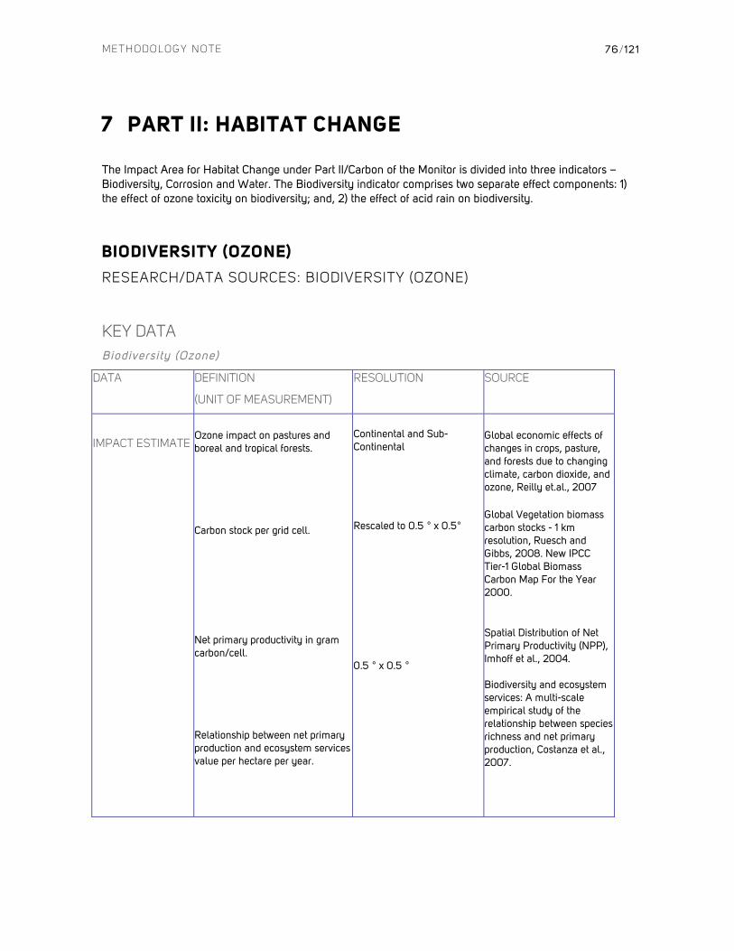
METHODOLOGY NOTE

76 /121

7 PART II: HABITAT CHANGE

The Impact Area for Habitat Change under Part II/Carbon of the Monitor is divided into three indicators – Biodiversity, Corrosion and Water. The Biodiversity indicator comprises two separate effect components: 1) the effect of ozone toxicity on biodiversity; and, 2) the effect of acid rain on biodiversity.

BIODIVERSITY (OZONE)

RESEARCH/DATA SOURCES: BIODIVERSITY (OZONE)

KEY DATA

Biodiversity (Ozone)

DATA DEFINITION


RESOLUTION SOURCE

IMPACT ESTIMATE Ozone impact on pastures and boreal and tropical forests.

Carbon stock per grid cell.

Net primary productivity in gram carbon/cell.

Relationship between net primary production and ecosystem services value per hectare per year.

Continental and Sub-Continental Rescaled to 0.5 ° x 0.5° 0.5 ° x 0.5 °

Global economic effects of changes in crops, pasture, and forests due to changing climate, carbon dioxide, and ozone, Reilly et.al., 2007

Global Vegetation biomass carbon stocks - 1 km resolution, Ruesch and Gibbs, 2008. New IPCC Tier-1 Global Biomass Carbon Map For the Year 2000.

Spatial Distribution of Net Primary Productivity (NPP), Imhoff et al., 2004. Biodiversity and ecosystem services: A multi-scale empirical study of the relationship between species richness and net primary production, Costanza et al., 2007.

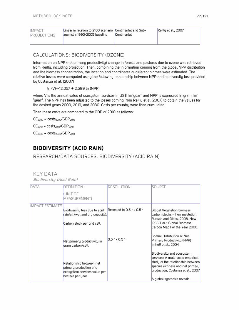
METHODOLOGY NOTE

77/121

IMPACT PROJECTIONS

Linear in relation to 2100 scenario against a 1990-2005 baseline

Continental and Sub-Continental

Reilly et al., 2007

CALCULATIONS: BIODIVERSITY (OZONE)

Information on NPP (net primary productivity) change in forests and pastures due to ozone was retrieved from Reilly, including projection. Then, combining the information coming from the global NPP distribution and the biomass concentration, the location and coordinates of different biomes were estimated. The relative losses were computed using the following relationship between NPP and biodiversity loss provided by Costanza et al, (2007)

ln (V)=-12.057 + 2.599 ln (NPP)

where V is the annual value of ecosystem services in US$ ha-1year-1 and NPP is expressed in gram ha-

1year-1. The NPP has been adjusted to the losses coming from Reilly et al (2007) to obtain the values for the desired years 2000, 2010, and 2030. Costs per country were then cumulated.


CE2000 = costs2000/GDP2010

CE2010 = costs2010/GDP2010

CE2030 = costs2030/GDP2010

BIODIVERSITY (ACID RAIN)

RESEARCH/DATA SOURCES: BIODIVERSITY (ACID RAIN)

KEY DATA Biodiversity (Acid Rain)

DATA DEFINITION


RESOLUTION SOURCE

IMPACT ESTIMATE Biodiversity loss due to acid rainfall (wet and dry deposits).

Carbon stock per grid cell.

Net primary productivity in gram carbon/cell.

Relationship between net primary production and ecosystem services value per hectare per year.

Rescaled to 0.5 ° x 0.5 ° 0.5 ° x 0.5 °

Global Vegetation biomass carbon stocks - 1 km resolution, Ruesch and Gibbs, 2008. New IPCC Tier-1 Global Biomass Carbon Map For the Year 2000.

Spatial Distribution of Net Primary Productivity (NPP) Imhoff et al., 2004.

Biodiversity and ecosystem services: A multi-scale empirical study of the relationship between species richness and net primary production, Costanza et al., 2007 A global synthesis reveals

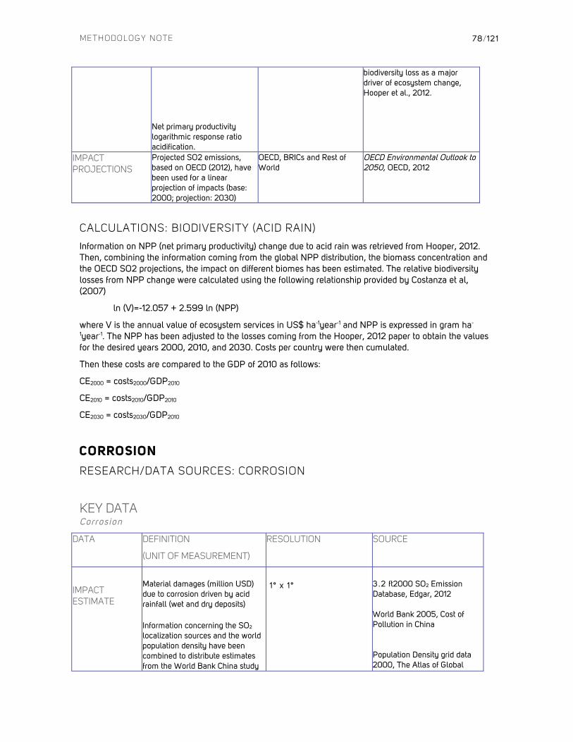
METHODOLOGY NOTE

78/121

Net primary productivity logarithmic response ratio acidification.

biodiversity loss as a major driver of ecosystem change, Hooper et al., 2012.

IMPACT PROJECTIONS

Projected SO2 emissions, based on OECD (2012), have been used for a linear projection of impacts (base: 2000; projection: 2030)

OECD, BRICs and Rest of World

OECD Environmental Outlook to 2050, OECD, 2012

CALCULATIONS: BIODIVERSITY (ACID RAIN)

Information on NPP (net primary productivity) change due to acid rain was retrieved from Hooper, 2012. Then, combining the information coming from the global NPP distribution, the biomass concentration and the OECD SO2 projections, the impact on different biomes has been estimated. The relative biodiversity losses from NPP change were calculated using the following relationship provided by Costanza et al, (2007)

ln (V)=-12.057 + 2.599 ln (NPP)

where V is the annual value of ecosystem services in US$ ha-1year-1 and NPP is expressed in gram ha-

1year-1. The NPP has been adjusted to the losses coming from the Hooper, 2012 paper to obtain the values for the desired years 2000, 2010, and 2030. Costs per country were then cumulated.


CE2000 = costs2000/GDP2010

CE2010 = costs2010/GDP2010

CE2030 = costs2030/GDP2010

CORROSION

RESEARCH/DATA SOURCES: CORROSION

KEY DATA Corrosion

DATA DEFINITION


RESOLUTION SOURCE

IMPACT ESTIMATE

Material damages (million USD) due to corrosion driven by acid rainfall (wet and dry deposits)

Information concerning the SO2 localization sources and the world population density have been combined to distribute estimates from the World Bank China study

1° x 1°

3.2 ft2000 SO2 Emission Database, Edgar, 2012 World Bank 2005, Cost of Pollution in China Population Density grid data 2000, The Atlas of Global

METHODOLOGY NOTE

79/121

globally

Two different mechanism are taken into account: dry and wet deposition of the most important acidifying gases (SO2)

0.5°x0.5° Conservation: Changes, Challenges, and Opportunities to Make a Difference, Hoekstra et al., 2010.

PROJECTED IMPACT

Projected SO2 emissions, based on OECD (2012), have been used to project the impacts (base: 2000; projection: 2030)

OECD, BRICs and Rest of World

OECD Environmental Outlook to 2050, OECD , 2012

CALCULATIONS: CORROSION

The SO2 emission grid generated from the Edgar database was first overlapped with country geographic information and then further overlapped with the population density grid. A worldwide robust estimation of the acid rain material damage was calculated by assuming the damage occurring on infrastructure with a particular SO2 concentration will follow a specific trend as provided by the World Bank, 2005 paper. Costs were normalized to the losses in China for the year 2003 provided by the World Bank paper. The 2050 SO2 emissions projections were obtained using the data from the OECD paper.

With a linear approach the losses are computed for the years 2000, 2010 and 2030:

costs2000_i = costs2000_i (base value model)

costs2010_i = Yi x 2/6+ costs2000_i

costs2030_i = Yi x 4/6+ costs2000_i

Where i represents the cell i and Y_i is the mean SO2 emission change provided by the OECD paper.


CE2000 = costs2000/GDP2010

CE2010 = costs2010/GDP2010

CE2030 = costs2030/GDP2010

WATER

RESEARCH/DATA SOURCES: WATER

KEY DATA Water

DATA DEFINITION


RESOLUTION SOURCE

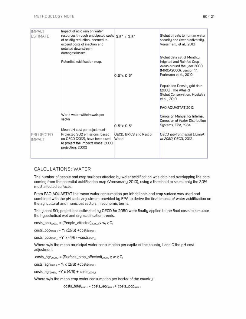
METHODOLOGY NOTE

80/121

IMPACT ESTIMATE

Impact of acid rain on water resources through anticipated costs of acidity reduction, deemed to exceed costs of inaction and entailed downstream damages/losses. Potential acidification map. World water withdrawals per sector Mean pH cost per adjustment

0.5° x 0.5°

0.5°x 0.5°

0.5°x 0.5°

Global threats to human water security and river biodiversity, Vorosmarty et al,. 2010 Global data set of Monthly Irrigated and Rainfed Crop Areas around the year 2000 (MIRCA2000), version 1.1, Portmann et al., 2010

Population Density grid data (2000), The Atlas of Global Conservation, Hoekstra et al., 2010. FAO AQUASTAT,2012 Corrosion Manual for Internal Corrosion of Water Distribution Systems, EPA, 1984

PROJECTED IMPACT

Projected SO2 emissions, based on OECD (2012), have been used to project the impacts (base: 2000; projection: 2030)

OECD, BRICS and Rest of World


CALCULATIONS: WATER

The number of people and crop surfaces affected by water acidification was obtained overlapping the data coming from the potential acidification map (Vorosmarty 2010), using a threshold to select only the 30% most affected surfaces.

From FAO AQUASTAT the mean water consumption per inhabitants and crop surface was used and combined with the pH costs adjustment provided by EPA to derive the final impact of water acidification on the agricultural and municipal sectors in economic terms.

The global SO2 projections estimated by OECD for 2050 were finally applied to the final costs to simulate the hypothetical wet and dry acidification trends.

costs_pop2000_i = (People_affected)2000_i x wi x Ci

costs_pop2010_i = Yi x(2/6) +costs2000_i

costs_pop2030_i =Yi x (4/6) +costs2000_i

Where wi is the mean municipal water consumption per capita of the country I and Ci the pH cost adjustment.

costs_agr2000_i = (Surface_crop_affected)2000_i x wi x Ci

costs_agr2010_i = Yi x (2/6) +costs2000_i

costs_agr2030_i =Yi x (4/6) + costs2000_i

Where wi is the mean crop water consumption per hectar of the country i.

costs_totalyear_i = costs_agryear_i + costs_popyear_i

METHODOLOGY NOTE

81/121


CE2000 = costs2000/GDP2010

CE2010 = costs2010/GDP2010

CE2030 = costs2030/GDP2010

8 PART II: HEALTH IMPACT

The Health Impact section of Part II/Carbon of the Monitor comprises adjustments in the predicted evolution of disease burdens as for the health section of Part I of the Monitor, where relevant. Likewise, the same system was used for calculating health costs as outlined in the Health impact section of Part I/Climate of this methodological note. The Health Impact section of Part II of the Monitor comprises the following indicators:

• Air Pollution

• Indoor Smoke

• Occupational Hazards

Each indicator aggregates relevant sub-indicators combining different health effects as detailed below.

AIR POLLUTION The Monitor’s indicator for Indoor Smoke The Indicator on the health impact of Air Pollution linked to emissions of greenhouse gases which are a principal cause of climate change is broken down from its composite form into two sub-indicators, one covering Urban Air Pollution as defined by the WHO, and a second expanding the problematic to Asthma with similar root causes (notably tropospheric ozone toxicity). These sub-indicators are detailed below.

RESEARCH/DATA SOURCES: AIR POLLUTION (URBAN)

KEY DATA Air Pollution (Urban)



RESOLUTION SOURCE

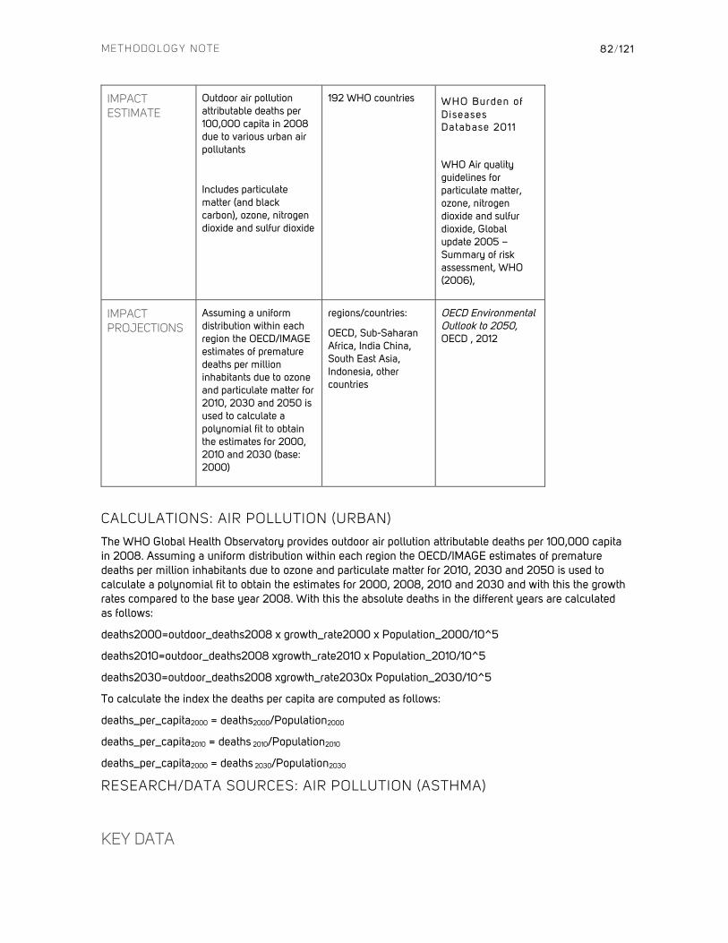
METHODOLOGY NOTE

82/121

IMPACT ESTIMATE

Outdoor air pollution attributable deaths per 100,000 capita in 2008 due to various urban air pollutants

Includes particulate matter (and black carbon), ozone, nitrogen dioxide and sulfur dioxide

192 WHO countries

WHO Burden of Diseases Database 2011

WHO Air quality guidelines for particulate matter, ozone, nitrogen dioxide and sulfur dioxide, Global update 2005 – Summary of risk assessment, WHO (2006),

IMPACT PROJECTIONS

Assuming a uniform distribution within each region the OECD/IMAGE estimates of premature deaths per million inhabitants due to ozone and particulate matter for 2010, 2030 and 2050 is used to calculate a polynomial fit to obtain the estimates for 2000, 2010 and 2030 (base: 2000)

regions/countries:

OECD, Sub-Saharan Africa, India China, South East Asia, Indonesia, other countries

OECD Environmental Outlook to 2050, OECD , 2012

CALCULATIONS: AIR POLLUTION (URBAN)

The WHO Global Health Observatory provides outdoor air pollution attributable deaths per 100,000 capita in 2008. Assuming a uniform distribution within each region the OECD/IMAGE estimates of premature deaths per million inhabitants due to ozone and particulate matter for 2010, 2030 and 2050 is used to calculate a polynomial fit to obtain the estimates for 2000, 2008, 2010 and 2030 and with this the growth rates compared to the base year 2008. With this the absolute deaths in the different years are calculated as follows:

deaths2000=outdoor_deaths2008 x growth_rate2000 x Population_2000/10^5

deaths2010=outdoor_deaths2008 xgrowth_rate2010 x Population_2010/10^5

deaths2030=outdoor_deaths2008 xgrowth_rate2030x Population_2030/10^5

To calculate the index the deaths per capita are computed as follows:

deaths_per_capita2000 = deaths2000/Population2000

deaths_per_capita2010 = deaths 2010/Population2010


RESEARCH/DATA SOURCES: AIR POLLUTION (ASTHMA)

KEY DATA

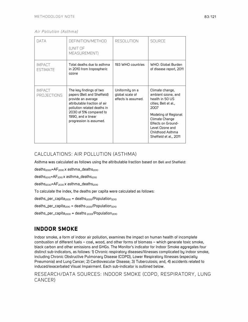
METHODOLOGY NOTE

83/121

Air Pollution (Asthma)



RESOLUTION SOURCE

IMPACT ESTIMATE

Total deaths due to asthma in 2010 from tropospheric ozone

193 WHO countries

WHO: Global Burden of disease report, 2011

IMPACT PROJECTIONS

The key findings of two papers (Bell and Sheffield) provide an average attributable fraction of air pollution related deaths in 2030 of 5% compared to 1990, and a linear progression is assumed.

Uniformity on a global scale of effects is assumed.

Climate change, ambient ozone, and health in 50 US cities; Bell et al., 2007

Modeling of Regional Climate Change Effects on Ground-Level Ozone and Childhood Asthma Sheffield et al., 2011

CALCULATIONS: AIR POLLUTION (ASTHMA)

Asthma was calculated as follows using the attributable fraction based on Bell and Sheffield:

deaths2000=AF2000 x asthma_deaths2010



To calculate the index, the deaths per capita were calculated as follows:

deaths_per_capita2000 = deaths2000/Population2010



INDOOR SMOKE

Indoor smoke, a form of indoor air pollution, examines the impact on human health of incomplete combustion of different fuels – coal, wood, and other forms of biomass – which generate toxic smoke, black carbon and other emissions and GHGs. The Monitor’s indicator for Indoor Smoke aggregates four distinct sub-indicators, as follows: 1) Chronic respiratory diseases/illnesses complicated by indoor smoke, including Chronic Obstructive Pulmonary Disease (COPD), Lower Respiratory Illnesses (especially Pneumonia) and Lung Cancer; 2) Cardiovascular Disease; 3) Tuberculosis; and, 4) accidents related to induced/exacerbated Visual Impairment. Each sub-indicator is outlined below.

RESEARCH/DATA SOURCES: INDOOR SMOKE (COPD, RESPIRATORY, LUNG CANCER)

METHODOLOGY NOTE

84/121

KEY DATA Indoor Smoke (COPD, Lower Respiratory Il lness, Lung Cancer)



RESOLUTION SOURCE

IMPACT ESTIMATE

Indoor air pollution attributable deaths per 100,000 capita – deaths primarily resulting from cooking and heating with solid fuels on open fires or traditional stoves that generate toxic indoor smoke containing a range of health-damaging pollutants, such as inhalable micro particles and carbon monoxide

192 WHO countries


WHO 2006, WHO Air quality guidelines for particulate matter, ozone, nitrogen dioxide and sulfur dioxide, Global update 2005 – Summary of risk assessment, WHO, 2006

IMPACT PROJECTIONS

Assuming a uniform distribution within each region the OECD/IMAGE estimates of premature deaths per million inhabitants due to indoor air pollution for 2010, 2030 and 2050 are used to calculate a polynomial fit to obtain the estimates for 2000, 2010 and 2030 (base: 2000)

regions/countries:

OECD, BRICs, Indonesia, South Africa, Sub-Saharan Africa, Other countries


RESEARCH/DATA SOURCES: INDOOR SMOKE (CARDIOVASCULAR)

KEY DATA Indoor Smoke (Cardiovascular)



RESOLUTION SOURCE

BASELINE Total deaths due to cardiovascular disease

193 WHO countries

WHO: Global Burden of disease report 2011

IMPACT ESTIMATE

Indoor air pollution attributable deaths per capita in 2010 (corresponds in degree to the AF for CVD under urban air pollution)

WHO regions

Indoor air pollution from biomass fuel smoke is a major health concern in the developing world; Fullerton et al., 2008

METHODOLOGY NOTE

85/121

IMPACT PROJECTIONS

Assuming that the deaths due to the diseases expand in tandem with the population growth rate – no adjustment made for declining reliance on traditional forms of heating and cooling which cause indoor smoke hazards

Global/184 countries

UN Population Division - Medium-fertility variant, 2010-2100, 2012

RESEARCH/DATA SOURCES: INDOOR SMOKE (TUBERCULOSIS)

KEY DATA Indoor Smoke (Tuberculosis)



RESOLUTION SOURCE

BASELINE Total deaths due to tuberculosis disease

193 WHO countries


IMPACT ESTIMATE

Indoor air pollution attributable deaths per capita in 2010:

Mishra establishes that India has a considerable AF of 0.51 on indoor smoke for Tuberculosis. To calculate global AFs India is used as a benchmark.

Country specific, extrapolated with benchmark

Biomass Cooking Fuels and Prevalence of Tuberculosis in India; Mishra , 1999a

IMPACT PROJECTIONS




CALCULATIONS: INDOOR SMOKE (TUBERCULOSIS)

To account for differences in exposure to indoor smoke total deaths per capita in country (i) due to indoor smoke / total deaths per capita in India due to indoor smoke is calculated.

A 1:1 relationship is assumed between overall impact (total deaths per cap due to indoor smoke) and the AF.

This ratio is multiplied by 0.51, where the maximum AF is set to 0.51. The implication is that a lower relative exposure will result in a lower AF; while a higher exposure will be set equal to India (it is not reasonable to assume higher AFs close to or above 1).

RESEARCH/DATA SOURCES: INDOOR SMOKE (VISUAL IMPAIRMENT)

KEY DATA Indoor Smoke (Visual Impairment)

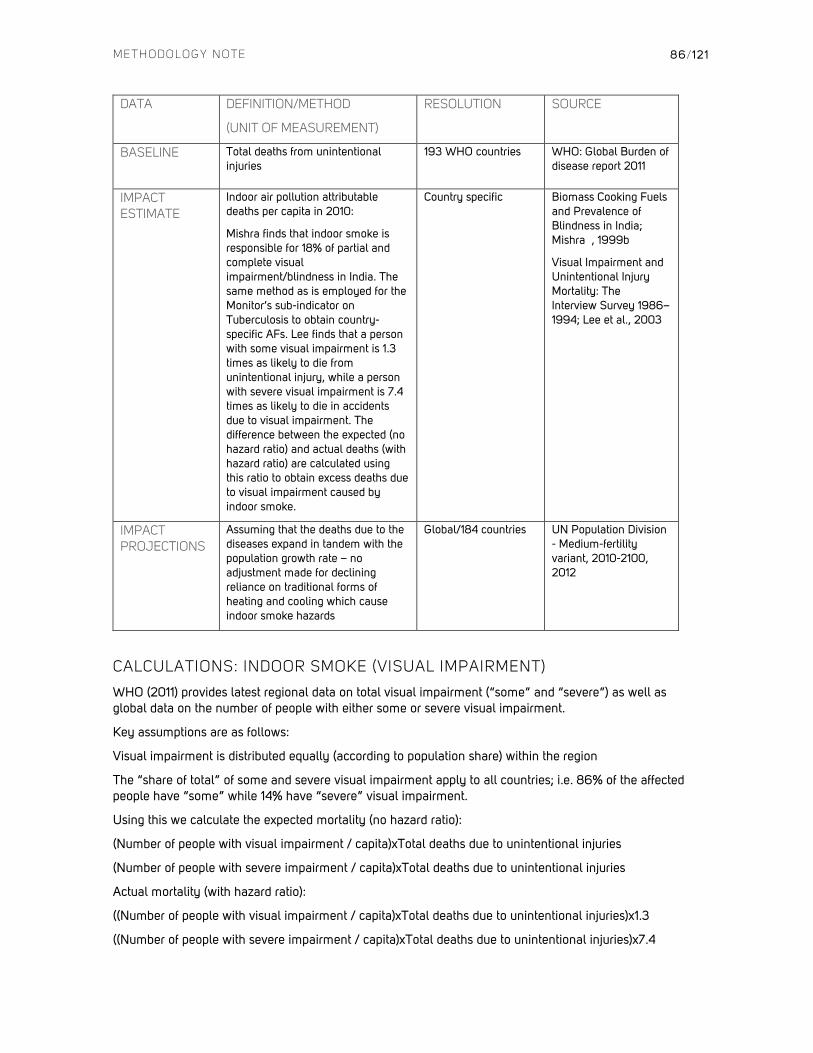
METHODOLOGY NOTE

86/121



RESOLUTION SOURCE

BASELINE Total deaths from unintentional injuries

193 WHO countries

WHO: Global Burden of disease report 2011

IMPACT ESTIMATE

Indoor air pollution attributable deaths per capita in 2010:

Mishra finds that indoor smoke is responsible for 18% of partial and complete visual impairment/blindness in India. The same method as is employed for the Monitor’s sub-indicator on Tuberculosis to obtain country-specific AFs. Lee finds that a person with some visual impairment is 1.3 times as likely to die from unintentional injury, while a person with severe visual impairment is 7.4 times as likely to die in accidents due to visual impairment. The difference between the expected (no hazard ratio) and actual deaths (with hazard ratio) are calculated using this ratio to obtain excess deaths due to visual impairment caused by indoor smoke.

Country specific

Biomass Cooking Fuels and Prevalence of Blindness in India; Mishra , 1999b

Visual Impairment and Unintentional Injury Mortality: The Interview Survey 1986–1994; Lee et al., 2003

IMPACT PROJECTIONS




CALCULATIONS: INDOOR SMOKE (VISUAL IMPAIRMENT)

WHO (2011) provides latest regional data on total visual impairment (“some” and “severe”) as well as global data on the number of people with either some or severe visual impairment.

Key assumptions are as follows:

Visual impairment is distributed equally (according to population share) within the region

The “share of total” of some and severe visual impairment apply to all countries; i.e. 86% of the affected people have “some” while 14% have “severe” visual impairment.

Using this we calculate the expected mortality (no hazard ratio):

(Number of people with visual impairment / capita)xTotal deaths due to unintentional injuries

(Number of people with severe impairment / capita)xTotal deaths due to unintentional injuries

Actual mortality (with hazard ratio):

((Number of people with visual impairment / capita)xTotal deaths due to unintentional injuries)x1.3

((Number of people with severe impairment / capita)xTotal deaths due to unintentional injuries)x7.4

METHODOLOGY NOTE

87/121

Excess deaths due to visual impairment caused by indoor smoke:

AF (0.18 for India)x((actual_some-expected_some)+( (actual_severe-expected_severe))

OCCUPATIONAL HAZARDS

The Monitor’s indicator for Occupation Hazards aggregates three distinct sub-indicators related to hazards stemming from workplaces closely related to high greenhouse gas emissions, as follows: 1) Asthma, from industry specific exposures; 2) COPD, for similar reasons; 3) Coal Workers Pneumoconiosis (CWP) and coal accidents that only concerns coal extraction professionals; and, 4) Stomach Cancer, which again is linked to industry specific exposures. Each sub-indicator is outlined below.

RESEARCH/DATA SOURCES: OCCUPATIONAL HAZARDS (ASTHMA & COPD)

KEY DATA Occupational Hazards (Asthma & COPD)



RESOLUTION SOURCE

BASELINE

Population employed in: Electricity, Transportation, Mining

Total deaths due to ASTHMA and COPD 2008

country specific

country specific

ILO LABORSTAT database, 2C Total Employment by Occupation

WHO burden of Disease, 2011

IMPACT ESTIMATE

Relative Risk, RRi or “Attributable Factors (AF)” for specific employment sectors

country specific WHO: Occupational airborne

Particulates, Driscoll et al., 2004

IMPACT PROJECTIONS

Deaths 2030 from COPD caused by workplace exposure using the deaths growth rates related to economic growth (minimum of Loncar-Mathers and the GDP-growth approach)

6 regions:

Afr ica, The Americas, Eastern Mediterranean, Europe, South-East Asia, Western Pacif ic

Projections of global mortality and burden of disease from 2002 to 2030, Mathers and Loncar, 2006

RESEARCH/DATA SOURCES: OCCUPATIONAL HAZARDS (CWP & COAL ACCIDENTS)

KEY DATA Occupational Hazards (CWP)



RESOLUTION SOURCE

BASELINE 2008 coal production (million tonnes) 71 (all coal producing) countries

2010 Survey if Energy Resources, World

METHODOLOGY NOTE

88/121

Energy Council (2010)

IMPACT ESTIMATE

We have precise CWP mortality figures (a lung disease due to coal particles) for Turkey and the US.

We assume that these CWP mortality figures represent the year 2008 (the year our coal production data dates to) and calculate the deaths/million tons ratio and round.

USA: 0.46 = 0.5 (represents all OECD producers)

Turkey: 1.41 = 1.5 (represents all non OECD)

2 countries Coal workers Pneumoconiosis: Mortality, CDCP , 2012b

Turkey: Evaluation of the risk of coal workers pneumoconiosis (CWP): A case study for the Turkish hardcoal mining; Aydin, 2010

IMPACT PROJECTIONS

Assuming a 1:1 relationship between production volume and deaths per million tons, the BP Energy Outlook 2030 is used to calculate deaths in 2000 and 2030

6 regions:

North America, S & C America, Europe & Eurasia, Middle East

Afr ica, Asia Pacif ic

Energy Outlook 2030, BP , 2012

KEY DATA Occupational Hazards (Coal accidents)



RESOLUTION SOURCE

BASELINE

2008 coal production (million tonnes)

Total coal extraction deaths 1999-2008

59 countries

9 countries

World Energy Council (2010), 2010 Survey if Energy Resources

International Mining Fatality Review database

IMPACT ESTIMATE

See below. Continental

Asia, Africa, South America, China, Eastern Europe, North America

BP (2012) Energy Outlook 2030

IMPACT PROJECTIONS


Regions:

Asia-Africa-South America-China; Eastern Europe; North America; rest with zero increase

BP (2012) Energy Outlook 2030

METHODOLOGY NOTE

89/121

RESEARCH/DATA SOURCES: OCCUPATIONAL HAZARDS (STOMACH CANCER)

KEY DATA Occupational Hazards (Stomach Cancer)



RESOLUTION SOURCE

BASELINE

2008 coal production (million tonnes)

Total stomach cancer deaths 2010

71 (all coal producing) countries

184 countries

World Energy Council (2010), 2010 Survey if Energy Resources


IMPACT ESTIMATE

A comprehensive study of the coal mining industry in the Netherlands, Swaen (1995), finds that the relative difference between “observed” and “expected” deaths due to stomach cancer among coal workers are 1.47. I.e. when controlling for social and other factors coal miners have a 47 pct. higher risk of dying from stomach cancer than the general population.

Same ratio for all coal producing countries

Swaen et al., 1995

IMPACT PROJECTIONS


4 regions:

Asia-Africa-South America-China; Eastern Europe; North America; rest with zero increase

Energy Outlook 2030, BP , 2012

CALCULATIONS: OCCUPATIONAL HAZARDS

ASTHMA AND COPD

• WHO provides “Relative Risk (RR)” that we use to calculate our risk factors or “Attributable Factors (AF)” for specific employment sectors for COPD and Asthma due to airborne particulates.

• ILO is the key source of labor statistics - COPD: Electricity, Mining, Transportation; Asthma: Mining, Transport

• WHO provides baseline deaths due to COPD and Asthma

• WHO provides regional projections for 2030

MINING SECTOR DATA

For mining sector data, only coal mining is considered. No global country specific database of employment

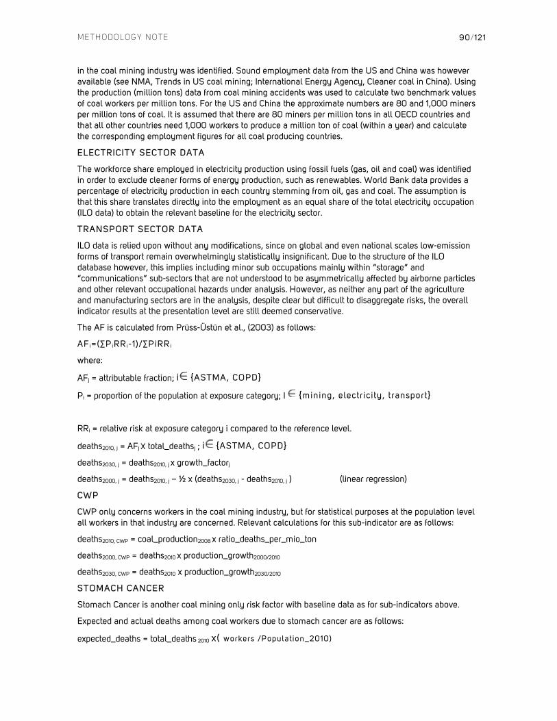
METHODOLOGY NOTE

90/121

in the coal mining industry was identified. Sound employment data from the US and China was however available (see NMA, Trends in US coal mining; International Energy Agency, Cleaner coal in China). Using the production (million tons) data from coal mining accidents was used to calculate two benchmark values of coal workers per million tons. For the US and China the approximate numbers are 80 and 1,000 miners per million tons of coal. It is assumed that there are 80 miners per million tons in all OECD countries and that all other countries need 1,000 workers to produce a million ton of coal (within a year) and calculate the corresponding employment figures for all coal producing countries.

ELECTRICITY SECTOR DATA

The workforce share employed in electricity production using fossil fuels (gas, oil and coal) was identified in order to exclude cleaner forms of energy production, such as renewables. World Bank data provides a percentage of electricity production in each country stemming from oil, gas and coal. The assumption is that this share translates directly into the employment as an equal share of the total electricity occupation (ILO data) to obtain the relevant baseline for the electricity sector.

TRANSPORT SECTOR DATA

ILO data is relied upon without any modifications, since on global and even national scales low-emission forms of transport remain overwhelmingly statistically insignificant. Due to the structure of the ILO database however, this implies including minor sub occupations mainly within “storage” and “communications” sub-sectors that are not understood to be asymmetrically affected by airborne particles and other relevant occupational hazards under analysis. However, as neither any part of the agriculture and manufacturing sectors are in the analysis, despite clear but difficult to disaggregate risks, the overall indicator results at the presentation level are still deemed conservative.

The AF is calculated from Prüss-Üstün et al., (2003) as follows:

AFi=(∑PiRRi-1)/∑PiRRi

where:

AFj = attributable fraction; i {ASTMA, COPD}

Pi = proportion of the population at exposure category; I {mining, electricity, transport}

RRi = relative risk at exposure category i compared to the reference level.

deaths2010, j = AFj X total_deathsj ; i {ASTMA, COPD}

deaths2030, j = deaths2010, j x growth_factorj

deaths2000, j = deaths2010, j – ½ x (deaths2030, j - deaths2010, j ) (linear regression)

CWP

CWP only concerns workers in the coal mining industry, but for statistical purposes at the population level all workers in that industry are concerned. Relevant calculations for this sub-indicator are as follows:

deaths2010, CWP = coal_production2008 x ratio_deaths_per_mio_ton

deaths2000, CWP = deaths2010 x production_growth2000/2010

deaths2030, CWP = deaths2010 x production_growth2030/2010

STOMACH CANCER

Stomach Cancer is another coal mining only risk factor with baseline data as for sub-indicators above.

Expected and actual deaths among coal workers due to stomach cancer are as follows:

expected_deaths = total_deaths 2010 x( workers /Populat ion_2010)

METHODOLOGY NOTE

91/121

actual_deaths = 1.47 x expected_deaths

And with this, the excess Stomach Cancer deaths due to coal mining is:

deaths2010 ,SC = actual_deaths - expected_deaths

deaths2000, SC = deaths2010 x production_growth2000/2010

deaths2030, SC = deaths2010 xproduction_growth2030/2010

AGGREGATION

Relevant calculations aggregating the sub-indicators are as follows:

deaths2000 = deaths2000,ASTHMA + deaths2000,COPD + deaths2000,CWP + deaths2000,SC



To calculate the index we calculated the deaths per capita as follows:

deaths_per_capita2000 = deaths2000/population2000



S K I N C A N C E R KEY DATA Occupational Hazards (Skin Cancer)



RESOLUTION SOURCE

BASELINE

Total skin cancer deaths 2010

Continental . 56 countr ies

184 Countr ies


IMPACT ESTIMATE A comprehensive model focused on the skin cancer evolution in Australia under different scenarios.

Australia-Focused Model

Health Impacts of Climate Change and Ozone Depletion: An Ecoepidemiologic

Modeling Approach,. Martens, 1998

METHODOLOGY NOTE

92/121

IMPACT PROJECTIONS

Modeling the carcinogenic risk of artificial UV sources and the use of indoor tanning facilities.

Global study Exposure To Artificial UV Radiation And Skin Cancer 2005 WHO International Agency For Research On Cancer

Martens , 1998

The work of Martens (1998) was used to assess the impact of UV exposure, caused by the ozone depletion by CFCs and halocarbons, on skin cancer incidence in the period 2000-2030.

The Australian values have been used as a proxy to describe the grown rate for all the 56 countries choosing a scenario that includes an aging population with a 50% decrease in UV exposure.

Death2000_i=WHOdeath_i x Skin_cancer_rate_2000_modeled



A 5% correction to epurate the data from the additional skin cancer cases due to artificial UV exposure have been applied to the final result. (IARC).

Finally to calculate the index the death per capita are computed as follows:




METHODOLOGY NOTE

93/121

9 PART II: INDUSTRY STRESS

The Industry Stress section of the Monitor’s Part II/Carbon covers three different sectoral effects by indicators: agriculture, fisheries and forestry. These are independently aggregate of a number of different effects comprising sub-indicators for these three areas. Agriculture is comprised of four sub-indicators: 1) acid rain, 2) ozone toxicity, 3) global dimming, and, 4) carbon fertilization. Fisheries is comprised of two sub-indicators: 1) marine fisheries (ocean acidification), and, 2) in-land fisheries (acidification/acid rain). Forestry comprises two sub-indicators, as follows: 1) ozone toxicity, and, 2) acid rain.

AGRICULTURE (ACID RAIN)

RESEARCH/DATA SOURCES: AGRICULTURE (ACID RAIN)

KEY DATA Agriculture (Acid Rain)

DATA DEFINITION


RESOLUTION SOURCE

IMPACT ESTIMATE

Production losses in agriculture (million USD) due to acid rain

Information concerning the SO2 localization sources and the world population density have been combined to distribute estimates from the World Bank China study globally

Two different mechanism are taken into account: dry and wet deposition of the most important acidifying gases (SO2)

1°x 1°

0.5°x 0.5°

3.2 ft2000 SO2 Emission Database , Edgar, (2012)

The World Bank (2005), Cost of pollution in China


IMPACT PROJECTION

Linear (base: 2000; projection: 2030) OECD, BRICs and Rest of World

OECD (2012), Environmental Outlook to 2050

CALCULATIONS: AGRICULTURE (ACID RAIN)

The SO2 emission grid coming from the Edgar database was first overlapped with country geographic information and then further overlapped with the monthly irrigated and rainfed crop map (MIRCA2000). A worldwide robust estimation of the acid rain agricultural damage was calculated by assuming the damage occurring on crops with a particular SO2 concentration will follow a specific trend provided by World Bank,

METHODOLOGY NOTE

94/121

2005. Costs were normalized to the losses in China for the year 2003 provided by the World Bank. The 2050 SO2 emissions projections were obtained using the data from the OECD paper.

With a linear approach the losses are calculated for the years 2000, 2010 and 2030:

costs2000 = 1/6 x costs2050




CE2000 = costs2000/GDP2010

CE2010 = costs2010/GDP2010

CE2030 = costs2030/GDP2010

AGRICULTURE (OZONE)

RESEARCH/DATA SOURCES: AGRICULTURE (OZONE)

KEY DATA Agriculture (Ozone)

DATA DEFINITION


RESOLUTION SOURCE

IMPACT ESTIMATE Losses to agricultural production (million USD) due to tropospheric ozone

Country level

Global crop yield reductions due to surface ozone exposure: 2. Year 2030 potential crop production losses and economic damage under two scenarios of O3 pollution, Avnery et al., 2011.

IMPACT PROJECTIONS

The 2010 and 2030 projections use a linear interpolation assuming no losses in 1990

As above Averny et al., 2011

CALCULATIONS: AGRICULTURE (OZONE)

The costs for 2030 are provided by Avnery (2011). With a linear approach the losses are calculated for the years 2000, 2010 and 2030:

costs2000 = ¼ x costs2030


costs2030 = costs2030 (provided by the paper)

METHODOLOGY NOTE

95/121


CE2000 = costs2000/GDP2010

CE2010 = costs2010/GDP2010

CE2030 = costs2030/GDP2010

AGRICULTURE (GLOBAL DIMMING)

RESEARCH DATA/SOURCES: AGRICULTURE (GLOBAL DIMMING)

KEY DATA Agriculture (Global Dimming)

DATA DEFINITION


RESOLUTION SOURCE

IMPACT ESTIMATE Losses to agricultural production (million USD) due to (polluting) atmospheric brown clouds

Using the data from Hansen describing the variation in (w/m2) of incident solar radiation due to black carbon and other gases related to anthropic activities the global radiation balance was assessed

With this new corrected value the approx. agricultural losses have been assessed using estimates in UNEP 2008

0.5° x 0.5° 5° x 4°


Impacts of Atmospheric Brown Clouds on Agriculture Agrawal et al., UNEP 2008 Clear sky incident solar radiation (1850-2030) "Dangerous human-made interference with climate: A GISS modelE study" by Hansen et al., 2007 FAOSTAT: gross production value for all crops, 2012

IMPACT PROJECTIONS

Linear projection from 1850 (no effect) to 2030

5° x 4°

Hansen et. al., 2007

CALCULATIONS: AGRICULTURE (GLOBAL DIMMING)

Using the model provided by Hansen et al, the change in clear sky incident solar radiation was analyzed on a global scale. These changes are in general and principally attributed to greenhouse gases (black carbon, ozone, etc.). Information regarding the trends in crop growth due to change in radiation was retrieved from UNEP 2008. The map containing crop density was then overlapped with the new solar radiation field and losses were projected. The crop value was obtained from FAOSTAT.

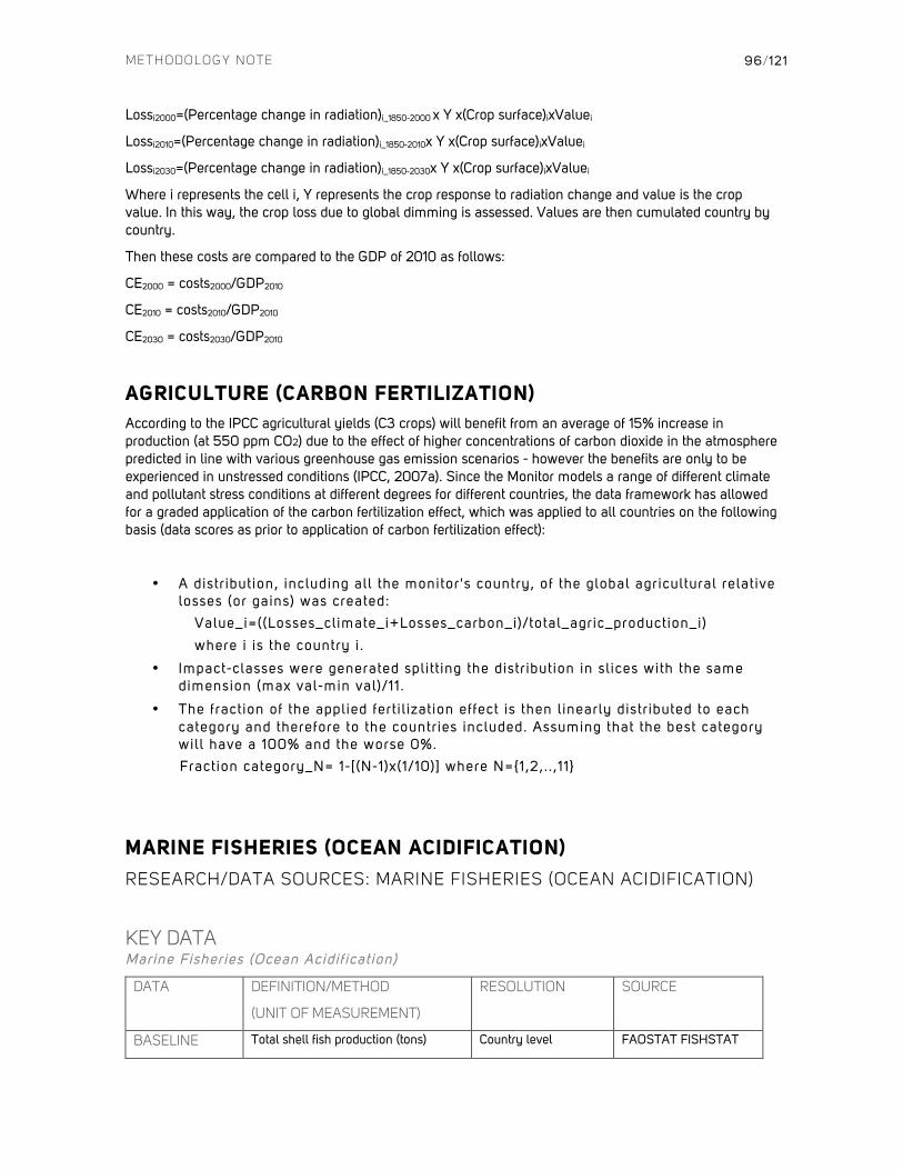
METHODOLOGY NOTE

96/121

Lossi2000=(Percentage change in radiation)i_1850-2000 x Y x(Crop surface)ixValuei

Lossi2010=(Percentage change in radiation)i_1850-2010x Y x(Crop surface)ixValuei

Lossi2030=(Percentage change in radiation)i_1850-2030x Y x(Crop surface)ixValuei

Where i represents the cell i, Y represents the crop response to radiation change and value is the crop value. In this way, the crop loss due to global dimming is assessed. Values are then cumulated country by country.


CE2000 = costs2000/GDP2010

CE2010 = costs2010/GDP2010

CE2030 = costs2030/GDP2010

AGRICULTURE (CARBON FERTILIZATION)

According to the IPCC agricultural yields (C3 crops) will benefit from an average of 15% increase in production (at 550 ppm CO2) due to the effect of higher concentrations of carbon dioxide in the atmosphere predicted in line with various greenhouse gas emission scenarios - however the benefits are only to be experienced in unstressed conditions (IPCC, 2007a). Since the Monitor models a range of different climate and pollutant stress conditions at different degrees for different countries, the data framework has allowed for a graded application of the carbon fertilization effect, which was applied to all countries on the following basis (data scores as prior to application of carbon fertilization effect):

• A distribution, including all the monitor's country, of the global agricultural relative losses (or gains) was created:

Value_i=((Losses_climate_i+Losses_carbon_i)/total_agric_production_i)

where i is the country i .

• Impact-classes were generated splitt ing the distribution in slices with the same dimension (max val-min val)/11.

• The fraction of the applied ferti l ization effect is then linearly distributed to each category and therefore to the countries included. Assuming that the best category will have a 100% and the worse 0%.

Fraction category_N= 1-[(N-1)x(1/10)] where N={1,2,. . ,11}

MARINE FISHERIES (OCEAN ACIDIFICATION)

RESEARCH/DATA SOURCES: MARINE FISHERIES (OCEAN ACIDIFICATION)

KEY DATA Marine Fisheries (Ocean Acidif ication)



RESOLUTION SOURCE

BASELINE Total shell fish production (tons) Country level FAOSTAT FISHSTAT

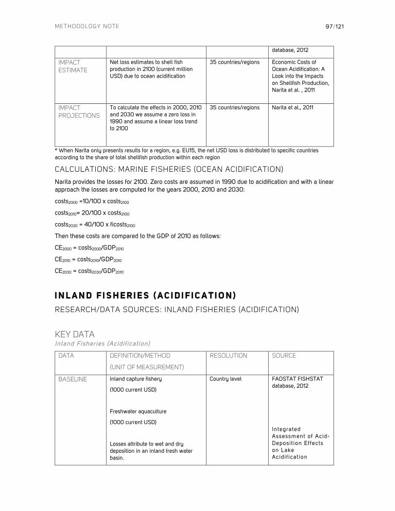
METHODOLOGY NOTE

97/121

database, 2012

IMPACT ESTIMATE

Net loss estimates to shell fish production in 2100 (current million USD) due to ocean acidification

35 countries/regions Economic Costs of Ocean Acidification: A Look into the Impacts on Shellfish Production, Narita et al. , 2011

IMPACT PROJECTIONS

To calculate the effects in 2000, 2010 and 2030 we assume a zero loss in 1990 and assume a linear loss trend to 2100

35 countries/regions Narita et al., 2011

* When Narita only presents results for a region, e.g. EU15, the net USD loss is distributed to specific countries according to the share of total shellfish production within each region

CALCULATIONS: MARINE FISHERIES (OCEAN ACIDIFICATION)

Narita provides the losses for 2100. Zero costs are assumed in 1990 due to acidification and with a linear approach the losses are computed for the years 2000, 2010 and 2030:

costs2000 =10/100 x costs2100

costs2010= 20/100 x costs2100

costs2030 = 40/100 x ficosts2100


CE2000 = costs2000/GDP2010

CE2010 = costs2010/GDP2010

CE2030 = costs2030/GDP2010

I N L A N D F I S H E R I E S ( A C I D I F I C A T I O N )

RESEARCH/DATA SOURCES: INLAND FISHERIES (ACIDIFICATION)

KEY DATA Inland Fisheries (Acidif ication)



RESOLUTION SOURCE

BASELINE

Inland capture fishery

(1000 current USD)

Freshwater aquaculture

(1000 current USD)

Losses attribute to wet and dry deposition in an inland fresh water basin.

Country level FAOSTAT FISHSTAT database, 2012

Integrated Assessment of Acid-Deposit ion Effects on Lake Acidif icat ion

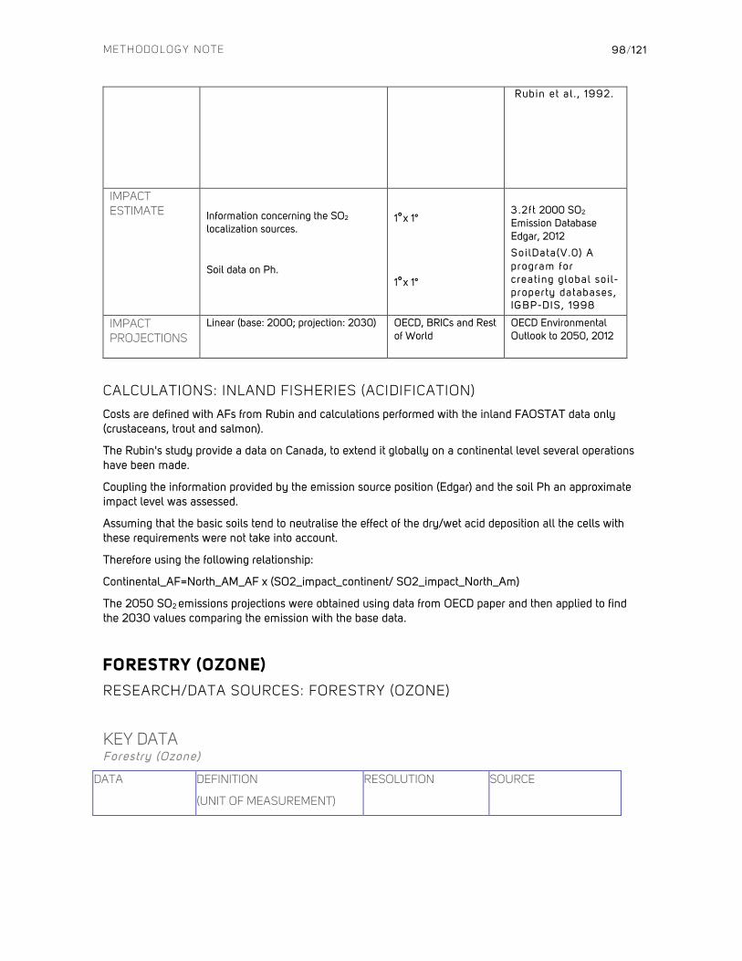
METHODOLOGY NOTE

98/121

Rubin et al . , 1992.

IMPACT ESTIMATE

Information concerning the SO2 localization sources.

Soil data on Ph.

1°x 1°

1°x 1°

3.2ft 2000 SO2 Emission Database Edgar, 2012

SoilData(V.0) A program for creating global soil-property databases, IGBP-DIS, 1998

IMPACT PROJECTIONS


OECD Environmental Outlook to 2050, 2012

CALCULATIONS: INLAND FISHERIES (ACIDIFICATION)

Costs are defined with AFs from Rubin and calculations performed with the inland FAOSTAT data only (crustaceans, trout and salmon).

The Rubin's study provide a data on Canada, to extend it globally on a continental level several operations have been made.

Coupling the information provided by the emission source position (Edgar) and the soil Ph an approximate impact level was assessed.

Assuming that the basic soils tend to neutralise the effect of the dry/wet acid deposition all the cells with these requirements were not take into account.

Therefore using the following relationship:

Continental_AF=North_AM_AF x (SO2_impact_continent/ SO2_impact_North_Am)

The 2050 SO2 emissions projections were obtained using data from OECD paper and then applied to find the 2030 values comparing the emission with the base data.

FORESTRY (OZONE)

RESEARCH/DATA SOURCES: FORESTRY (OZONE)

KEY DATA Forestry (Ozone)

DATA DEFINITION


RESOLUTION SOURCE

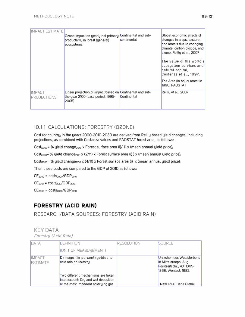
METHODOLOGY NOTE

99/121

IMPACT ESTIMATE Ozone impact on yearly net primary productivity in forest (general) ecosystems.

Continental and sub-continental

Global economic effects of changes in crops, pasture, and forests due to changing climate, carbon dioxide, and ozone, Reilly et al., 2007 The value of the world’s ecosystem services and natural capital , Costanza et al . , 1997.

The Area (in ha) of forest in 1990, FAOSTAT

IMPACT PROJECTIONS

Linear projection of impact based on the year 2100 (base period: 1995-2005)

Continental and sub-Continental

Reilly et al., 2007

10.1.1 CALCULATIONS: FORESTRY (OZONE)

Cost for countryi in the years 2000-2010-2030 are derived from Reilly based yield changes, including projections, as combined with Costanza values and FAOSTAT forest area, as follows:

Costi2000= % yield change2100i x Forest surface area (i)/ 11 x (mean annual yield price)i

Costi2010= % yield change2100 x (2/11) x Forest surface area (i) ) x (mean annual yield price)i

Costi2030= % yield change2100 x (4/11) x Forest surface area (i) x (mean annual yield price)i


CE2000 = costs2000/GDP2010

CE2010 = costs2010/GDP2010

CE2030 = costs2030/GDP2010

FORESTRY (ACID RAIN)

RESEARCH/DATA SOURCES: FORESTRY (ACID RAIN)

KEY DATA Forestry (Acid Rain)

DATA DEFINITION


RESOLUTION SOURCE

IMPACT ESTIMATE

Damage ( in percentage)due to acid rain on forestry

Two different mechanisms are taken into account: Dry and wet deposition of the most important acidifying gas

Ursachen des Waldsterbens in Mitteleuropa. Allg. Forstzeitschr., 43: 1365-1368, Wentzel, 1982.

. New IPCC Tier-1 Global

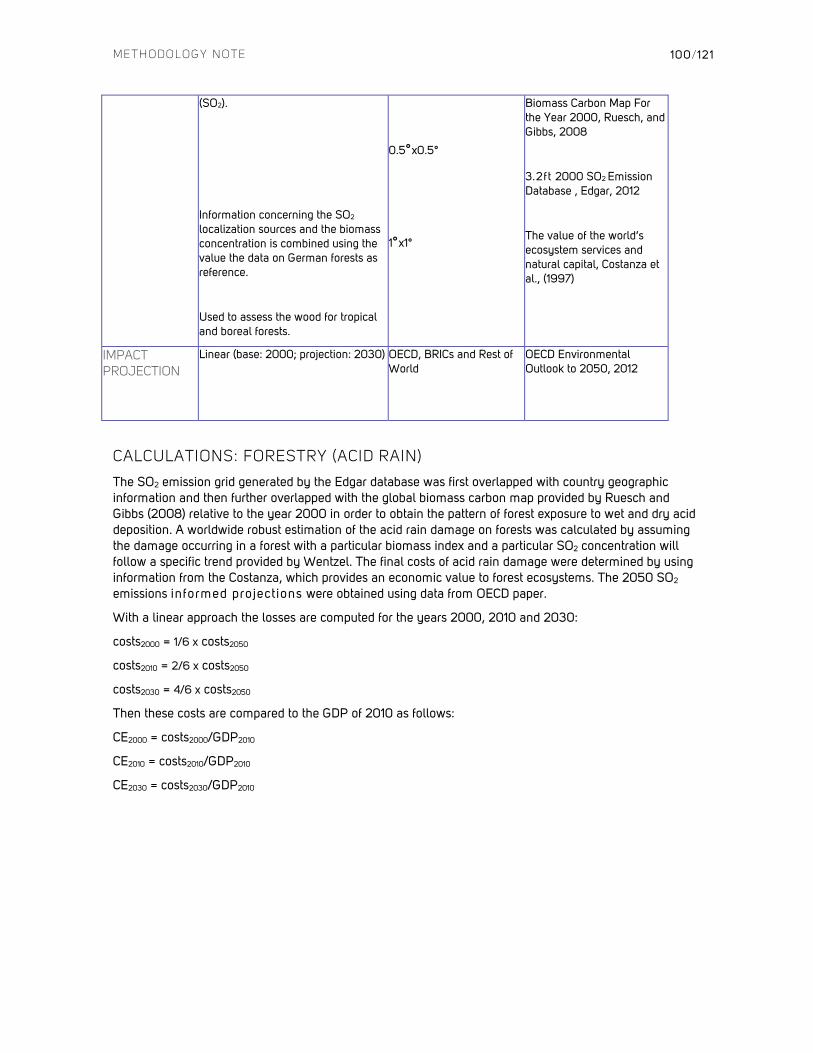
METHODOLOGY NOTE

100/121

(SO2).

Information concerning the SO2 localization sources and the biomass concentration is combined using the value the data on German forests as reference.

Used to assess the wood for tropical and boreal forests.

0.5°x0.5°

1°x1°

Biomass Carbon Map For the Year 2000, Ruesch, and Gibbs, 2008

3.2ft 2000 SO2 Emission Database , Edgar, 2012

The value of the world’s ecosystem services and natural capital, Costanza et al., (1997)

IMPACT PROJECTION


OECD Environmental Outlook to 2050, 2012

CALCULATIONS: FORESTRY (ACID RAIN)

The SO2 emission grid generated by the Edgar database was first overlapped with country geographic information and then further overlapped with the global biomass carbon map provided by Ruesch and Gibbs (2008) relative to the year 2000 in order to obtain the pattern of forest exposure to wet and dry acid deposition. A worldwide robust estimation of the acid rain damage on forests was calculated by assuming the damage occurring in a forest with a particular biomass index and a particular SO2 concentration will follow a specific trend provided by Wentzel. The final costs of acid rain damage were determined by using information from the Costanza, which provides an economic value to forest ecosystems. The 2050 SO2

emissions informed projections were obtained using data from OECD paper.

With a linear approach the losses are computed for the years 2000, 2010 and 2030:





CE2000 = costs2000/GDP2010

CE2010 = costs2010/GDP2010

CE2030 = costs2030/GDP2010

9 CLIMATE CHANGE FINANCE

The following is a brief log of data sources, methods and assumptions relied upon to create a comprehensive database of climate change financing up to 2010.

DATA SOURCES

In order to obtain a complete picture of climate change mitigation and adaptation two complementary data sources were used. The primary source was the OECD creditor reporting system. The supplementary source of information was drawn on for multi-lateral funds from individual funds’ public documentation/websites. Private finance is only obtainable through wide-ranging estimates available in third party publications.

OECD CREDITOR REPORTING SYSTEM

The OECD’s Creditor Reporting System (CRS) is a system for measuring Official Development Assistance (ODA) as reported by government donors and members of the OECD Development Assistance Committee (DAC). Aid in support of climate-related objectives is also tracked through detailed project-level reporting by OECD/DAC members against the so-called “Rio markers” for, amongst others, climate change adaptation and mitigation (prior to 2010 there was only a climate change marker and not a separate marker for adaptation and mitigation – so both were contained in the same marker prior to 2010). The Rio maker for climate change has been active since 1998. The latest data available for Rio markers is for 2010 (as at mid-2012), although preliminary estimates of overall ODA are available for 2011. Aid activities/flows can either be marked as “Principal objective” or “Significant objective” à If not otherwise stated, all calculations in the Monitor only include “Principal objective” aid activities.

The key assumptions for only factoring in Principal objective and not any resources for Significant objective are as follows:

• It is not customary to analyze sectoral ODA data as per the system used for Rio marker reporting given that in normal practice only one sector is ever mentioned, this means that sectoral analysis automatically excludes some activities that do relate to sectors, since only the main activity focus is logged

• Under the Rio marker system these activities would have been carried out were it not for interest in climate change – therefore in relation to Fast Start Finance commitments the resources likely stretch any definition of “new” or “additional”

• There is far lesser volume of resources labeled Significant than Principal

• There is no way to gauge what degree of focus is attributable to climate change, it could be as low as 5% or less

• Principal objective resources are neither 100% targeted towards climate change, since projects/programmes need only have climate change as a principal focus, and that the activity would not have been undertaken were it not for the interest in climate change

• Analysis has shown that reporting under Significant objective is much less rigorous than for

Principal objective, including a greater degree of so-called “over-coding” or misrepresentation of the objectives of projects

While the system is not ideal, excluding Significant objective from the analysis therefore minimizes double counting and erroneous data, providing a more measured viewpoint of resource flows on climate change.

The main database for Rio marker data are the Rio marker tables called “Full list of climate change mitigation and adaptation aid activities, 2010” and “Full list of climate change mitigation aid activities, 2007-2009” on http://www.oecd.org/document/6/0,3746,en_2649_34421_43843462_1_1_1_1,00.html that provided information on all climate change aid activities by the OECD donor countries and the European Union marked as mitigation and/or adaptation.

In addition, data from the bulk downloads was drawn upon [http://stats.oecd.org/Index.aspx?datasetcode=CRS1# à export à related files à CRS 2010.zip and CRS 2009.zip] that include all aid activities by the OECD donor countries (not only climate change) and by multilateral funds and institutions that report to the CRS system (World Bank institutions, multilateral development banks etc). Besides the donors already included in the Rio marker tables the bulk downloads include aid activities under the Rio markers for mitigation and adaptation for:

• IDA: reports on Mitigation, but only “Significant objective”. Started reporting in 2010 but made it retrospective.

• GEF: reports on Mitigation “Principal Objective” but only since 2010.

• Nordic Development Fund: reports on Mitigation and Adaptation (Principal and Significant Objective)

In cases where there are aid activities marked “Principal Objective” only, these are used to determine the total amount of climate change funding (the case for the GEF and the Nordic Dev. Fund). In the case of the IDA where, there is not a single aid activity marked as “Principal Objective”, in which case 40% of the amount marked as “Significant objective” is applied only.

In the case of the IDA, the resulting amount is divided by the total sum of aid activities providing the % share for climate change.

à 1.56% in 2010 and 1.30% in 2009

This percentage is then multiplied by the donor countries’ contribution (commitments) to the IDA (obtained from the CRS online system).

In case of the GEF: Based on the “Proposed Indicative Resource Envelope for GEF-5” (as reported in table 8 of “Summary of Negotiations Fifth Replenishment of the GEF”, May 2010) approximately 32% of total GEF-5 fund replenishment will go towards the Climate Change focus area. Whilst cumulative funding decisions, as reported in GEF Trust Fund Trustees' Reports, fluctuate around this figure, on the advice of GEF, due to a lack of more detailed available information this data is used to approximate replenishments towards the climate change focal area.

Thus, the donor countries´ climate change funding through the GEF is calculated as 32% as their total commitment to the GEF (obtained from the CRS online system).

In case of the Nordic Dev. Fund the data from the CRS bulk download was used to determine the share for mitigation and adaptation aid activities (for 2010). These percentages are then applied to the Nordic countries´ contributions to the fund (baseline: paid-in capital during the respective calendar year).

MULTI-LATERAL FUNDS

Supplementary information on multi-lateral funds concerns the following entities:

• From individual funds’ websites, annual reports and financial statement

• Adaptation Fund, Least Developed Countries Fund, Special Climate Change Fund, Climate Investment Funds, Congo Basin Forest Fund, Global Climate Change Alliance, Forest Carbon Partnership Facility, UN REDD Programme

Specific calculations are made to integrate the two data sets, using the below variables as follows:

b) Amounts from Data source 1 (GEF and IDA, see calculation method above)

c) Amounts from Data source 1 (Nordic Dev. Fund) and Data source 2 (see list of funds above)

d) Amounts from Data source 2 (CER sales of Adaptation fund)

a) Difference between amounts from Data source 1 (total contributions from donor countries and European Union) minus amounts from Data source 2 (contributions from donor countries and European Union to multilateral funds)

Total: a) + b) + c) + d)

à This is done because it is assumed that the CRS reporting includes contributions to multilateral funds.

à In the case of most funds a detailed assessment (whether the contributions to the fund are included in the CRS data) was undertaken with varying results. In most cases some countries included their contributions in their Rio marker reporting, although not all.

10 BIBLIOGRAPHY A d a m o e t a l . ( 2 0 1 1 ) Adamo S., S. Trzaska, G. Yetman, J. del Corral, M. Thomson, and C. Perez (2011)

Integration of Demographic, Climate, and Epidemiological Factors in the Modeling of Meningococcal Meningitis Epidemic Occurrence in Niger.

Poster presented at the 2011 Annual Meeting of the Population Association of America in Washington, D.C., March 30–April 1 .

Retrieved: http://www.ciesin.org/documents/adamo-model-meningoccal_paa_mar2011.pdf

A g r a w a l e t a l . ( 2 0 0 8 )

M. Agrawal, M. Auffhammer, U.K. Chopra, L. Emberson, M. Iyngararasan, N. Kalra, M.V. Ramana, V. Ramanathan, A.K. Singh and J. Vincent (2008) Impacts of Atmospheric Brown Clouds on Agriculture Part I I of Atmospheric Brown Clouds: Regional Assessment Report with Focus on Asia Nairobi, Kenya: United Nations Environment Programme

A v n e r y e t a l . ( 2 0 1 1 )

Avnery S., D.L. Mauzerall, J. Liu, L.W. Horowitz (2011)

Global Crop Yield Reductions due to Surface Ozone Exposure: 1 . Year 2000 Crop Production Losses and Economic Damage

Atmospheric Environment , vol. 45, pp. 2284-2296.

A y d i n ( 2 0 1 0 ) H. Aydin (2010)

Evaluation of the risk of coal workers pneumoconiosis (CWP): A case study for the Turkish hardcoal mining Scientif ic Research and Essays , vol. 5, no. 21, pp. 3289-3297.

B a u m e r t a n d S e l m a n ( 2 0 0 3 )

Baumert K. and Selman M (2003) Data Note: Heating and Cooling Degree Days World Resources Institute

B a u m g a r t n e r e t a l . ( 2 0 1 1 ) S. Baumgartner, M. A. Drupp, J.M. Munz, J. N. Meya and M.F.Quuas (2003)

Income Distribution and Will ingness to pay for Ecosystem Services http://www.bioecon-network.org/pages/13th_2011/Baumgaertner.pdf

B e l l e t a l . ( 2 0 0 7 )

Michelle L. Bell, Richard Goldberg, Christian Hogrefe, Patrick L. Kinney, Kim Knowlton,

Barry Lynn, Joyce Rosenthal, Cynthia Rosenzweig, Jonathan A. Patz

Climate change, ambient ozone, and health in 50 US cit ies Climatic Change , vol. 82, no. 1, pp. 61-76.

B h a r a t h a n d T u r n e r ( 2 0 0 9 )

Bharath A.K. and Turner R.J. (2009) Impact of climate change on skin cancer

Journal of the Royal Society of Medicine , vol. 102, no. 6, pp. 215–218.

B P ( 2 0 1 2 ) BP (2012)

BP Energy Outlook 2030

C A P P ( 2 0 1 1 )

Canadian Association of Petroleum Production (2011) Crude oil : Forecasts, Markets and Pipelines CAPP

C D C P ( 2 0 1 2 ) Centers for Disease Control and Prevention

Various resources: Data & Statistics http://www.cdc.gov/DataStatistics/

C D C P ( 2 0 1 2 b )

Centers for Disease Control and Prevention (2012) Work related lung diseases surveillance system

Coal Workers Pneumoconiosis Mortality http://www.cdc.gov/DataStatistics/

C E D R E ( 2 0 1 2 )

Centre of Documentation, Research and Experimentation on Accidental Water Pollution Spills http://www.cedre.fr/en/spill/alphabetical-classif ication.php

C e n t e r f o r T a n k s h i p E x c e l l e n c e Center for Tankship Excellence

CTX version 4.6 Retrieved: http://www.c4tx.org/ctx/job/cdb/do_flex.html

C e r e s ( 2 0 1 0 ) Ceres (2010) Canada’s Oil Sands Shrinking Window of Opportunity Boston, MA, Ceres, Inc.

Retrieved: http://www.ceres.org/resources/reports/oil-sands-2010/view C h e u n g e t a l . ( 2 0 1 0 )

Will iam W. L. Cheung, Vicky W. Y. Lam, Jorge L. Sarmiento, Kelly Kearney, Reg Watson, Dirk Zeller, and Daniel Pauly (2010)

Large-scale redistribution of maximum fisheries catch potential in the global ocean under climate change Global Change Biology , vol. 16, no. 11, pp. 24-35.

C I A ( 2 0 1 2 )

CIA (2012) The World Factbook Retrieved: https://www.cia.gov/library/publications/the-world-factbook/

C I E S I N W e b s i t e Center for International Earth Science Information Network (CIESIN)

Socioeconomic Data and Applications Center http://sedac.ciesin.columbia.edu/

C l i n e ( 2 0 0 7 )

Will iam R. Cline (2007) Global Warming and Agriculture: Impact Estimates by Country Washington, DC: Center for Global Development.

C o r t i e t a l . ( 2 0 0 9 ) T. Corti , V. Muccione, P. Köllner-Heck, D. Bresch, and S. I . Seneviratne (2009)

Simulating past droughts and associated building damages in France Hydrology and Earth System Sciences Discussions , vol. 6, no. 2, pp. 1463–1487.

C o s t a n z a e t a l . ( 1 9 9 7 )

Robert Costanza, Ralph d’Arge, Rudolf de Groot, Stephen Farber, Monica Grasso, Bruce Hannon, Karin Limburg, Shahid Naeem, Robert V. O’Neill , Jose Paruelo, Robert G. Raskin, Paul Sutton, & Marjan van den Belt (1997) The value of the world’s ecosystem services and natural capital

Nature , vol. 387.

C o s t a n z a e t a l . ( 2 0 0 7 ) R Costanza, B Fisher, K Mulder, S Liu, T Christopher (2007)

Biodiversity and ecosystem services: A multi-scale empirical study of the relationship between species richness and net primary production Ecological Economics , vol. 61, no. 2-3, pp. 478-491.

C R E D / E M - D A T C R E D ( 2 0 1 2 )

Center for Research on the Epidemiology of Disasters (2012)

EM DAT – The International Disasters Database Retrieved: http://www.emdat.be/advanced-search

C u r r i e r o a l . ( 2 0 0 2 )

Frank C. Curriero, Karlyn S. Heiner, Jonathan M. Samet, Scott L. Zeger, Lisa Strug and Jonathan A. Patz (2002)

Temperature and Mortality in 11 Cit ies of the Eastern United States American Journal of Epidemiology , Vol. 155, no. 1, pp. 80-87.

D I V A ( 2 0 0 3 )

DINAS-COAST (2003) Dynamic Interactive Vulnerabil ity Assessment D o n a t e t a l . ( 2 0 1 1 )

Donat M.G., G. C. Leckebusch, S. Wild, and U. Ulbrich (2011)

Future changes in European winter storm losses and extreme wind speeds inferred from GCM and RCM multi-model simulations

Natural Hazards and Earth System Sciences , vol. 11, no. 5, pp 1351-1370.

D o u g l a s – W e s t w o o d ( 2 0 1 0 ) Douglas-Westwood/ New York (2010) Global Deepwater Prospects-2010 Presentation for the Deep Offshore Technology International Conference held in Houston, Texas, 2 February 2010 D r i s c o l l e t a l . ( 2 0 0 4 )

Tim Driscoll, Kyle Steenland, Deborah Imel Nelson, James Leigh (2004)

Occupational airborne particulates: Assessing the environmental burden of disease at national and local levels Environmental Burden of Disease Series, no. 7. Geneva, Switzerland: World Health Organization

E C L A C ( 2 0 1 1 )

Economic Commission for Latin America and the Caribbean (ECLAC) (2011)

An Assessment of the Economic Impact of Climate Change on the Tourism Sector in Barbados United Nations ECLAC

E D G A R ( 2 0 1 2 ) Emission Database for Global Atmospheric Research (EDGAR)

EDGAR 3.2 Fast Track 2000 dataset (32FT2000) PBL Netherlands Environmental Assessment Agency

http://131.224.244.83/en/themasites/edgar/emission_data/edgar_32ft2000/index.html

E M - D A T C R E D - See: CRED (above)

E n e r g y I n f o r m a t i o n A d m i n i s t r a t i o n W e b s i t e ( 2 0 1 2 ) Energy Information Administration Website

Various sources

E P A ( 2 0 1 0 ) Environmental Protection Agency (2010)

Various resources http://www.epa.gov/enviro/index.html

E P A ( 1 8 9 4 ) Environmental Protection Agency (1894) Corrosion Manual for the Internal Corrosion of water Distribution System E t k i n ( 2 0 0 4 )

Etkin, Dagmar Schmidt (2004)

Modeling Oil Spill Response and Damage Costs. In Proceedings of the 5th Biennial Freshwater Spills Symposium Washington, DC: US Environmental Protection Agency

E u s k i r c h e n e t a l . ( 2 0 0 6 )

E.S. Euskirchen, A.D. McGuire, D.W. Kicklighter, Q. Zhuang, J.S. Clein, R.J. Dargaville, D.G. Dye, J.S. Kimball, K.C. McDonald, J.M. Melil lo, V.E. Romanovsky, and N.V. Smith (2006)

Importance of recent shifts in soil thermal dynamics on growing season length, productivity, and carbon sequestration in terrestrial high-latitude ecosystems Global Change Biology , vol. 12, no. 4, pp. 731–750

F A O ( 2 0 1 2 )

FAO AQUASTAT Database http://www.fao.org/nr/water/aquastat/dbases/index.stm

F A O F I S H S T A T ( 2 0 1 2 ) FAO FISHSTAT (2012)

FishStat Plus Database http://www.fao.org/fishery/statistics/software/fishstat/en

F A O S T A T ( 2 0 1 2 )

FAOSTAT (2012) Various Resources

http://faostat.fao.org/

F u l l e r t o n e t a l . ( 2 0 0 8 )

Fullerton D.G., Bruce N., and Gordon S.B. (2008)

Indoor air pollution from biomass fuel smoke is a major health concern in the developing world

Transactions of the Royal Society of Tropical Medicine and Hygiene , vol. 102, no. 9, pp. 843-851.

G e o s p a t i a l I n f o r m a t i o n A u t h o r i t y o f J a p a n e t a l . ( 2 0 0 3 )

Geospatial Information Authority of Japan, Chiba University and collaborating organizations (2003)

Global Map V.1, Vegetation (Percent tree cover), F Modis Data 2003. International Steering Committee for Global Mapping (ISCGM). Global Mapa Data Download Service. Retrieved: http://www.iscgm.org/GM_ptc.html G e o w o r l d m a p

Geoworldmap Geobytes’ GeoWorldmap Database Retrieved: http://www.geobytes.com/FreeServices.htm

H a n s e n e t a l . ( 2 0 0 7 )

J. Hansen, M. Sato, R. Ruedy, P. Kharecha, A. Lacis, R. Miller, L. Nazarenko, K. Lo, G. A. Schmidt, G. Russell, I . Aleinov, S. Bauer, E. Baum, B. Cairns, V. Canuto, M. Chandler, Y. Cheng, A. Cohen, A. Del Genio, G. Faluvegi, E. Fleming, A. Friend, T. Hall, C. Jackman, J. Jonas, M. Kelley, N. Y. Kiang, D. Koch, G. Labow, J. Lerner, S. Menon, T. Novakov, V. Oinas, Ja. Perlwitz, Ju. Perlwitz, D. Rind, A. Romanou, R. Schmunk, D. Shindell, P. Stone, S. Sun, D. Streets, N. Tausnev, D. Thresher, N. Unger, M. Yao, and S. Zhang (2007)

Dangerous human-made interference with climate: A GISS modelE study Atmospheric Chemistry and Phys ics, vol. 7, pp. 2287-2312.

H i l l e t a l . ( 2 0 0 4 )

David J. Hill , J. Mark Elwood, Dallas R. English (2004) Prevention of Skin Cancer Kluwer Academic Publishers: the Netherlands

H o e k s t r a e t a l . ( 2 0 1 0 )

Jonathan M. Hoekstra, Jennifer L. Molnar, Michael Jennings, Carmen Revenga, Mark D. Spalding, Timothy M. Boucher, James C. Robertson, Thomas J. Heibel, and Katherine Ell ison (2010)

The Atlas of Global Conservation: Changes, Challenges, and Opportunities to Make a Difference Berkeley: University of California Press

Retrieved: http://preview.grid.unep.ch/index.php?preview=home&lang=eng

H o o p e r e t a l . ( 2 0 1 2 )

David U. Hooper, E. Carol Adair, Bradley J. Cardinale, Jarrett E. K. Byrnes, Bruce A. Hungate, Kristin L. Matulich, Andrew Gonzalez, J. Emmett Duffy, Lars Gamfeldt, Mary I.

O’Connor (2012)

A global synthesis reveals biodiversity loss as a major driver of ecosystem change Nature I G B P - D I S ( 1 9 9 8 )

IGBP Global Soils Data Task (1998) SoilData(V.0) A program for creating global soil-property databases I k u t a e t a l . ( 2 0 0 0 )

K. Ikuta, T. Yada, S. Kitamura, N. Branch, F. Ito, F., M. Yamagichi, M., T. Nishimura, T. Kaneko, M. Nagae, A. Ishimatsu, M. Iwata (2000) Effects of Acidif ication on Fish Reproduction

UJNR Technical Report , No. 28.

I L O ( 2 0 1 2 ) International Labour Organization (2012)

Various resources: LABORSTA Database http://laborsta.i lo.org/

I M F ( 2 0 1 1 )

IMF (2011) World Economic Outlook (2011 data and statistics)

International Monetary Fund

I m h o f f e t a l . ( 2 0 0 4 )

Imhoff Marc L., Lahouari Bounoua, Taylor Ricketts, Colby Loucks, Robert Harriss, and Will iam T. Lawrence (2004)

Spatial Distribution of Net Primary Productivity (NPP) Data distributed by the Socioeconomic Data and Applications Center (SEDAC)

http://sedac.ciesin.columbia.edu/es/hanpp.html

I n t e r n a t i o n a l E n e r g y A g e n c y ( 2 0 1 0 ) International Energy Agency (2010)

Energy Statistics and Balances of Non-OECD Countries, Energy Statistics of OECD Countries, and Energy Balances of OECD Countries Retrieved 2010: http://www.iea.org/stats/index.asp

I n t e r n a t i o n a l M i n i n g F a t a l i t y R e v i e w ( 2 0 1 2 )

International Mining Fatality Review (2012) NSW Government

Retrieved: http://www.resources.nsw.gov.au/safety/publications/statistical-publications/international-mining-fatality-review

I P C C ( 2 0 0 7 )

IPPC (2007) Fourth Assessment Report : Climate Change 2007 (AR4) Geneva, Switzerland: GRID Arendal & Intergovernmental Panel on Climate Change I s a a c a n d v a n V u u r e n ( 2 0 0 9 )

Morna Isaac and Detlef P. van Vuuren (2009)

Modeling global residential sector energy demand for heating and air conditioning in the context of climate change

Energy Policy , vol. 37, no. 2, pp. 507-521.

J o n k e r e n e t a l . ( 2 0 1 1 ) Jonkeren Olaf, Rietveld Piet, van Ommeren Jos (2011)

Climate Change and Inland Waterway Transport: Welfare Effects of Low Water Levels on the River Rhine Journal of Transport Economics and Policy , vol. 41, no. 3, pp. 387-411.

J u s t i n & W o o d ( 2 0 0 8 )

Sheffield Justin and Eric F. Wood (2008)

Projected changes in drought occurrence under future global warming from multi – model, multiscenario, IPCC AR4 simulations

Climate Dynamics , vol. 31, no.1, pp 79 – 105.

K a h n ( 2 0 0 5 ) Matthew E. Kahn (2005)

The Death Toll from Natural Disasters: The Role of Income, Geography, and Institutions The review of economics and statistics, vol. 87, no: 2, pp. 271-284

K h a r i n e t a l . ( 2 0 0 7 )

Viatcheslav V. Kharin, Francis W. Zwiers, Xuebin Zhang, and Gabriele C. Hegerl (2007)

Changes in Temperature and Precipitation Extremes in the IPCC Ensemble of Global Coupled Model Simulations

Journal of Climate , vol. 20, pp. 1419-1444.

K i n d e r m a n n e t a l . ( 2 0 0 6 ) G. E Kindermann, M. Obersteiner, E. Rametsteiner and I. McCallum (2006) Predicting the deforestation-trend under different carbon-prices Carbon Balance and Management , vol. 1, no.15 K j e l l s t r o m e t a l . ( 2 0 0 9 ) Kjellstrom T., Kovats R.S., Lloyd S.J., Holt T., Tol R.S. (2009)

The Direct Impact of Climate Change on Regional Labor Productivity Archives of Environmental & Occupational Health , vol. 64, no. 4.

K n u t t i e t a l . ( 2 0 0 8 )

R. Knutti , M. R. Allen, P. Friedlingstein, J. M. Gregory, G. C. Hegerl, G. A. Meehl, M.

Meinshausen, J. M. Murphy, G.-K. Plattner, S. C. B. Raper, T. F. Stocker, P. A. Stott, H. Teng, and T. M. L. Wigley (2008)

A Review of Uncertainties in Global Temperature Projections over the Twenty-First Century Journal of Climate , vol. 21, no. 11, pp. 2651–2663.

K r a w c h u k e t a l . ( 2 0 0 9 )

Meg A. Krawchuk, Max A. Moritz, Marc-André Parisien, Jeff Van Dorn, Katharine Hayhoe (2009) Global Pyrogeography: the Current and Future Distribution of Wildfire

PLoS ONE , vol. 4, no. 4.

L a r s e n a n d G o l d s m i t h ( 2 0 0 7 ) Peter Larsen and Scott Goldsmith (2007)

How much Might Climate Change Add to Future Costs for Public Infrastructure? Understanding Alaska , Research Summary, no. 8.

Institute of Social and Economic Research, University of Alaska Anchorage

L e e e t a l . ( 2 0 0 3 ) Lee David J·, Gómez-Marín Orlando, Lam Byron L, Zheng D Diane (2003)

Visual impairment and unintentional injury mortality: the National Health Interview Survey 1986-1994 American journal of ophthalmology , vol. 136, no. 6, pp. 1152-1154.

L e h n e r e t a l . ( 2 0 0 1 )

Bernhard Lehner, Gregor Czisch, Sara Vassolo (2001) Europe’s Hydropower Potential Today and in the Future

In: Lehner B. et al. : EuroWasswer: Model-based assessment of European water resources and hydrology in the face of global change. Kassel World Water Series 5, Ch. 8, pp. 8.1-8.22. Kassel, Germany: Center for Environmental Systems Research, University of Kassel

M a c e e t a l . ( 2 0 0 5 ) G.Mace, H. Masundire and J. Baill ie (2005). Biodiversity in: R. Hassan, R. Scholes and N. Ash (eds . ) : Ecosystems and Human Well-being: Current State and Trends (Chapter 4) Millenium Ecosystem Assessment

M a r t e n s ( 1 9 9 8 ) W.J.M. Martens (1998)

Health Impacts of Climate Change and Ozone Depletion: An Ecoepidemiologic Modeling Approach Environmental Health Perspectives , vol. 106, Supp.1, pp. 241-251

M a t h e r s a n d L o n c a r ( 2 0 0 6 )

Mathers CD, Loncar D. (2006) Projections of global mortality and burden of disease from 2002 to 2030

PLoS Medicine , vol. 3, no. 11.

M c K i n s e y a n d C o m p a n y ( 2 0 0 9 ) McKinsey and Company (2009)

Charting our Water Future: Economic Frameworks to Inform Decision Making Munich: 2030 Water Resources Group

M c M i c h a e l e t a l . ( 2 0 0 4 ) A. McMichael, D. Campbell-Lendrum, S. Kovats, S.Edwards, P. Wilkinson, T. Wilson, R.Nicholls, S. Hales, F. Tanser, D.Le Sueur, M. Schlesinger and N. Andronova (2004) Global Climate Change In: M. Ezzati M, A.D. Lopez, A. Roders and C.J.L. Murray (eds.) : Comparative Quantif ication of Health Risks, Global and Regional Burden of Disease Attributable to Selected Major Risk Factors (pp. 1543-1650) Geneva, Switzerland: World Health Organization M c N e i l a n d L e t s c h e r t ( 2 0 0 8 )

McNeil Michael A. and Letschert Virginie E. (2008)

Future Air Conditioning Energy Consumption in Developing Countries and what can be done about it : The Potential of Eff iciency in the Residential Sector.

Lawrence Berkeley National Laboratory

M e n d e l s o h n e t a l . ( 2 0 1 1 ) Mendelsohn R., Kerry E., and Chonabayashi S. (2011)

The Impact of Climate Change on Global Tropical Storms Damages Policy Research Working Paper no. 5562

The World Bank

M i l l e n n i u m E c o s y s t e m A s s e s s m e n t ( 2 0 0 5 ) Millennium Ecosystem Assessment (2005)

Millennium Assessment Report: Ecosystems and Human Well-Being Washington D.C., US: World Resources Institute

http://www.maweb.org/en/index.aspx

M i n ( 2 0 0 7 ) Hong-Ghi Min (2007)

Estimation of Labor Demand Elasticity for the RMSM-LP: Revised Minimum Standard Model for Labor and Poverty Module International Business & Economics Research Journal , vol. 6, no. 7, pp. 29-34.

M i s h r a e t a l . ( 1 9 9 9 a )

Mishra V.K., Retherford R.D., Smith K.R. (1999)

Biomass Cooking Fuels and Prevalence of Tuberculosis in India

International Journal of Infectious Diseases , vol. 3, no. 3, pp. 119-129.

M i s h r a e t a l . ( 1 9 9 9 b ) Mishra V.K., Retherford R.D., Smith K.R. (1999)

Biomass Cooking Fuels and Prevalence of Blindness in India Journal of Environmental Medicine , vol. 1, pp. 189-199.

M u e h l e n b a c h s e t a l . ( 2 0 1 1 ) Lucija Muehlenbachs, Mark A. Cohen, and Todd Gerarden (2011) Preliminary Empirical Assessment of Offshore Production Platforms in the Gulf of Mexico Resources for the Future Discussion Paper 10-66 Resources for the Future M u n i c h R e ( 2 0 1 1 )

NatCatSERVICE/Munich Re (2011) Statistics on natural catastrophes Retrieved: http://www.munichre.com/en/reinsurance/business/non-life/georisks/natcatservice/default.aspx

N a r i t a e t a l . ( 2 0 1 1 )

D. Narita, K. Rehdanz, R. Tol (2011) Economic Costs of Ocean Acidif ication: A Look into the Impacts on Shellf ish Production Working Paper no. WP391

Economic and Social Research Institute (ESRI)

N e l s o n e t a l . ( 2 0 0 1 ) Nelson, F. E., Anisimov O.A., and Shiklomanov N.I. (2001)

Model output from the 'frost index' permafrost model: variations in circumpolar frozen ground conditions and modeled future conditions Boulder, CO: National Snow and Ice Data Center

N o h a r a e t a l . ( 2 0 0 6 )

Daisuke Nohara, Akio Kitoh, Masahiro Hosaka, and Taikan Oki (2006) Impact of Climate Change on River Discharge Projected by Multimodel Ensemble

J. Hydrometeor , vol. 7, no 5., pp. 1076–1089.

O E C D ( 2 0 1 2 ) OECD (2012)

OECD Environmental Outlook to 2050: The Consequences of Inaction

O E C D ( 2 0 0 8 ) OECD (2008)

OECD Environmental Outlook to 2030.

O ’ R e i l l y e t a l . ( 2 0 0 3 )

O'Reilly C.M., Alin S.R., Plisnier P.D., Cohen A.S., McKee B.A. (2003) Climate Change decreases aquatic ecosystem productivity of Lake Tangayik, Africa

Nature , vol. 424, no. 6950, pp. 766–768.

P e d u z z i e t a l . ( 2 0 1 2 )

P. Peduzzi, B. Chatenoux, H. Dao, A. De Bono, C. Herold, J. Kossin, F. Mouton, and O. Nordbeck (2012)

Global trends in tropical cyclone risk Nature Climate Change , vol. 2, no. 6, pp. 89–294.

Retrieved 2010: http://www.eia.gov/

P e r e z - L o m b a r d e t a l . ( 2 0 0 8 ) Perez-Lombard L., Ortiz J. and Pout C. (2008)

A Review on Buildings Energy Consumption Information Energy and Buildings , vol. 40, no. 3, pp. 394-398.

P o r t m a n n e t a l . ( 2 0 1 0 )

Portmann, F.T., Siebert S., and Döll P. (2010)

Global Data Set of Monthly Irr igated and Rainfed Crop Areas Around the Year 2000 (MIRCA2000) Frankfurt, Germany: The Institute of Physical Geography, University of Frankfurt Retrieved: http://www.geo.uni-frankfurt.de/ipg/ag/dl/forschung/MIRCA/index.html

P r ü s s - Ü s t ü n e t a l . ( 2 0 0 3 )

Prüss-Üstün A, Woodward A, Corvalán C. (2003) Assessment of environmental burden of disease: introduction and methods. World Health Organization, Geneva

R e i l l y e t a l . ( 2 0 0 7 )

J. Reilly, S. Paltsev, B. Felzer, X. Wang, D. Kicklighter, J. Melil lo, R. Prinn, M. Sarofim, A. Sokolov, C. Wang (2007)

Global economic effects of changes in crops, pasture, and forests due to changing climate, carbon dioxide, and ozone Energy Policy , vol. 35, no. 11, pp. 5370-5383.

R i s k M e t r i c s G r o u p ( 2 0 1 0 )

Yulia Reuter, Doug Cogan, Dana Sasarean, Mario López Alcalá, and Dinah Koehler (2010) Canada’s Oil Sands Shrinking Window of Opportunity Boston, MA: CERES

R o s e n g r a n t e t a l . ( 2 0 0 2 )

Mark W. Rosegrant, Ximing Cai and Sarah A. Cline (2002) World water and Food to 2025 dealing with scarcity International Food Policy Research Institute R o t h b e r g e t a l . ( 2 0 0 8 )

Michael B. Rothberg, Sarah D. Haessler, and Richard B. Brown (2008) Complications of Viral Influenza

The American Journal of Medicine , no. 121, pp. 258-264.

R u b e l a n d K o t t e k ( 2 0 1 0 ) Franz Rubel and Markus Kottek (2010)

Observed and projected climate shifts 1901-2100 depicted by world maps of the Köppen-Geiger climate classif ication Meteorologische Zeitschrift , vol. 19, no. 2, pp. 135-141.

R u b i n e t a l . ( 1 9 9 2 )

E. S. Rubin , M.l J. Small, C. N. Bloyd and M. Henrion (1992)

Integrated Assessment of Acid-‐Deposition Effects on Lake Acidification Journal of Environmental Engineering, vol.118:1, pp. 120-134 R u e s c h a n d G i b b s ( 2 0 0 8 )

Ruesch Aaron and Holly K. Gibbs (2008) New IPCC Tier-1 Global Biomass Carbon Map for the Year 2000 Carbon Dioxide Information Analysis Center Oak Ridge, Tennessee: Oak Ridge National Laboratory

http://cdiac.ornl.gov

S h e f f i e l d e t a l . ( 2 0 1 1 ) Perry E. Sheffield, Kim Knowlton, Jessie L. Carr, and Patrick L. Kinney (2011)

Modeling of Regional Climate Change Effects on Ground-Level Ozone and Childhood Asthma American Journal of Preventive Medicine , vol. 41, no. 3, pp. 251-257.

S h e f f i e l d a n d W o o d ( 2 0 0 8 ) Justin Sheffield and Eric F. Wood (2008) Projected changes in drought occurrence under future global warming from multi – model, multiscenario, IPCC AR4 simulations Climate Dynamics , vol. 31, no.1, pp 79 – 105. S h i l p a k r e t a l ( 2 0 1 1 )

Raja Bhai Shilpakar, Narendra Man Shakya and Akira Hiratsuka (2011)

Impact of Climate Change on Snowmelt Runoff: A case study of Tamakoshi Basin in Nepal S t e i g e r ( 2 0 1 1 )

Steiger Robert (2011)

The impact of snow scarcity on ski tourism: an analysis of the record warm season 2006/2007 in Tyrol (Austria)

Tourism Review , vol. 66, no. 3, pp. 4 – 13.

S w a e n e t a l . ( 1 9 9 5 ) Swaen, G.M., Meijers, J.M.M. and Slangen, J.J.M. (1995)

Risk of gastric cancer in pneumoconiotic coal miners and the effect of respiratory impairment Occupational and Environmental Medicine , vol. 52, pp. 606-610.

T h o m a s e t a l . ( 2 0 0 4 )

Chris D. Thomas, Alison Cameron, Rhys E. Green, Michel Bakkenes, Linda J. Beaumont, Yvonne C. Coll ingham, Barend F. N. Erasmus, Marinez Ferreira de Siqueira, Alan Grainger, Lee Hannah, Lesley Hughes, Brian Huntley, Albert S. van Jaarsveld, Guy F. Midgley, Lera Miles, Miguel A. Ortega-Huerta, A. Townsend Peterson, Oliver L. Phill ips, and Stephen E. Will iams (2004) Extinction risk from climate change

Nature , vol. 427, no. 8, pp. 145-148

T o u l e m o n a n d B a r b i e r i ( 2 0 0 6 ) Toulemon Laurent and Magali Barbieri (2006)

The Mortality Impact of the August 2003 Heat Wave in France

Paper prepared for presentation at the 2006 Population of America Association Meeting, Los Angeles, March 30-April 1s t .

T r a b u c c o a n d Z o m e r ( 2 0 0 9 ) A.Trabucco and R.J. Zomer (2009) Database: Global Aridity Index (Global-Aridity) and Global Potential Evapo-Transpiration (Global-PET) Geospatial Database CGIAR Consortium for Spatial Information. Published online, available from the CGIAR-CSI GeoPortal at:http://www.csi.cgiar.org/ T r y s e ( 2 0 1 0 )

David Tryse (2010) Oil Spill Database

http://earth.tryse.net/oilspill .html

U N E C E ( 2 0 1 2 ) UNECE (2012) UNECE Statistical Database Retrieved: http://w3.unece.org/pxweb/ U N E C E ( 2 0 1 2 a ) UNECE (2012a)

Transport Division Database Carriage of goods by Inland Waterways (mill ion, tonne-km)

Retrieved: http://w3.unece.org/pxweb/dialog/varval.asp?ma=ZZZ_TRInlWaterTonKm_r&path=../database/STAT/40-TRTRANS/06-TRInlWater/&lang=1&ti=Carriage+of+goods+by+Inland+Waterways+%28mill ion%2C+tonne-km%29

U N E P / G R I D W e b s i t e

UNEP/GRID Website Global Risk Data Platform U n i t e d N a t i o n s C o m p e n d i u m o f H o u s i n g S t a t i s t i c s

United Nations Compendium of Housing Statistics Compendium of Human Settlements Statistics Retrieved: http://unstats.un.org/unsd/demographic/sconcerns/housing/housing2.htm

U n i t e d N a t i o n s S t a t i s t i c s D i v i s i o n ( 2 0 1 0 ) United Nations Statistics Division (2010)

UNSD Statistical Databases http://unstats.un.org/unsd/databases.htm U N P o p u l a t i o n D i v i s i o n ( 2 0 1 2 ) UN Department of Economic and Social Affairs Population Division (2012) World population Database Retrieved: http://www.un.org/esa/population/unpop.htm

U S C B W e b s i t e ( 2 0 1 2 ) United States Census Bureau Website (2012) Historical Census of Housing Tables. Home Values Census of Housing Retrieved:http://www.census.gov/hhes/www/housing/census/historic/values.html

U N S D ( 2 0 1 0 ) United Nations Statistics Division (2010) UNSD Statistical Databases http://unstats.un.org/unsd/databases.htm U N S D ( 2 0 1 2 ) United Nations Statistics Division (2012) UNSD Statistical Databases http://unstats.un.org/unsd/databases.htm

U S F o r e s t S e r v i c e ( 2 0 1 0 ) US Forest Service (2010) Potential vegetation distribution (average for 1961-1990) simulated using the MC1 model with CRU (TS 2.0) historical climate at a half degree spatial grain over the globe Data Basin Dataset, PNW Research Station Retrieved: http://www.arcgis.com/home/item.html?id=b2b92d2efcdc40738e9f1ce6ff49fde2

V a n N o o r t e t a l . ( 2 0 1 2 ) Van Noort S.P., Águas R., Ballesteros S., and Gomes M.G. (2012)

The role of weather on the relation between influenza and influenza-like il lness Journal of Theoretical Biology , no. 298, pp. 131–137

V a n a t ( 2 0 1 1 )

Vanat Laurent (2011)

2011 International report on mountain tourism - Overview of the key industry f igures for ski resorts May 2011 France: Institut de la Montagne

V ö r ö s m a r t y e t a l . ( 2 0 1 0 )

C.J. Vörösmarty, P.B. McIntyre, M.O. Gessner, D.Dudgeon, A.Prusevich, P.Green, S.Glidden, S.E. Bunn, C.A. Sullivan, C.Reidy Liermann, and P.M. Davies (2010)

Global threats to human water security and river biodiversity Nature , vol. 467, pp. 555-561.

W a c k e r e t a l . ( 2 0 0 6 )

John G. Wacker, Chen-Lung Yang, Chwen Sheu (2006) Productivity of production labor, non-production labor, and capital: An international study

International Journal of Production Economics , vol. 103, no. 2, pp. 863-872.

W a r d e t a l . ( 2 0 1 0 )

Phil ip J Ward, Kenneth M Strzepek, W Pieter Pauw, Luke M Brander, Gordon A Hughes and Jeroen C J H Aerts (2010)

Partial costs of global climate change adaptation for the supply of raw industrial and municipal water: a methodology and application Environmental Research Letters , vol. 5, no. 4.

W a u g h e t a l . ( 2 0 0 9 )

D. W. Waugh, L. Oman, S. R. Kawa, R. S. Stolarski, S. Pawson, A. R. Douglass, P. A. Newman, J. E. Nielsen (2009) Impacts of climate change on stratospheric ozone recovery

Geophysical Research Letters , vol. 36.

W e n t z e l ( 1 9 8 2 ) Ursachen des Waldsterbens in Mitteleuropa

Allgemeine Forst Zeitschrift , Vol. 43, pp. 1365-1368.

W h e e l e r ( 2 0 1 1 )

Wheeler David (2011) Quantifying Vulnerability to Climate Change: Implications for Adaptation Assistance CGD Working Paper 240

Washington, D.C.: Center for Global Development http://www.cgdev.org/content/publications/detail/1424759

W H O ( 2 0 0 4 ) Majid Ezzati, Alan D. Lopez, Anthony Rodgers and Christopher J.L. Murray (eds) (2004)

Comparative Quantif ication of Health Risks: Global and Regional Burden of Disease Attributable to Selected Major Risk Factors Geneva, Switzerland: World Health Organization

W H O ( 2 0 0 6 )

WHO (2006)

WHO Air quality guidelines for particulate matter, ozone, nitrogen dioxide and sulfur dioxide: Global update 2005. Summary of r isk assessment W H O B D D ( 2 0 1 1 )

Global Burden of Disease Data, 2011-data retrieved from: The Global Health Observatory (GHO) http://apps.who.int/ghodata/#

W H O W e b s i t e ( 2 0 1 2 ) WHO Website (2012)

Global Health Atlas Retrieved: http://apps.who.int/globalatlas/dataQuery/default.asp

W o r l d B a n k ( 2 0 1 2 ) World Bank (2012) Various resources: World DataBank http://data.worldbank.org/indicator W o r l d E c o n o m i c F o r u m ( 2 0 1 1 )

World Economic Forum (2011) The Global Economic Burden of Non-communicable Diseases A report by the World Economic Forum and the Harvard School of Public Health Geneva: World Economic Forum

W o r l d E n e r g y C o u n c i l ( 2 0 1 0 )

World Energy Council (2010) 2010 Survey of Energy Resources London, United Kingdom: World Energy Council

W o r l d P o p u l a t i o n P r o s p e c t s ( 2 0 1 1 ) World Population Prospects (2011)

Various resources Population Division, UN-DESA

http://esa.un.org/unpd/wpp/unpp/panel_population.htm

W o r l d R e s o u r c e s I n s t i t u t e W e b s i t e

World Resources Institute Website Reefs at Risk base GIS data Retrieved: http://www.wri.org/publication/content/7911 W o r l d R e s o u r c e s I n s t i t u t e W e b s i t e ( 2 0 1 2 ) World Resources Institute Website Reefs at Risk base GIS data Retrieved: http://www.wri.org/publication/content/7911

W T T C W e b s i t e World Travel and Tourism Council Website

Economic Data Search Tool Retrieved : http://www.wttc.org/research/economic-data-search-tool/

Z m e u r e a n u a n d R e n a u d ( 2 0 0 8 )

Zmeureanu R. and Renaud G. (2008) Estimation of Heating Energy Use of Existing Houses in a Future Climate: 2050 Vs 2007

Energy Policy , vol. 36, no. 1, pp. 303-310.

Z o m e r e t a l . ( 2 0 0 8 ) Robert J. Zomer, Antonio Trabucco, Deborah A. Bossio, Louis V. Verchot (2008)

Climate change mitigation: A spatial analysis of global land suitabil ity for clean development mechanism afforestation and reforestation Agriculture, Ecosystems and Environment , no. 126, pp. 67–80.

methodological documentation for the climate vulnerability …

Documents