méthode d'éléments finis mixtes :application aux équations de la
TRANSCRIPT

HAL Id: tel-00194195https://tel.archives-ouvertes.fr/tel-00194195
Submitted on 5 Dec 2007
HAL is a multi-disciplinary open accessarchive for the deposit and dissemination of sci-entific research documents, whether they are pub-lished or not. The documents may come fromteaching and research institutions in France orabroad, or from public or private research centers.
L’archive ouverte pluridisciplinaire HAL, estdestinée au dépôt et à la diffusion de documentsscientifiques de niveau recherche, publiés ou non,émanant des établissements d’enseignement et derecherche français ou étrangers, des laboratoirespublics ou privés.
Méthode d’éléments finis mixtes :application auxéquations de la chaleur et de Stokes instationnaires
Réda Korikache
To cite this version:Réda Korikache. Méthode d’éléments finis mixtes :application aux équations de la chaleur et de Stokesinstationnaires. Mathématiques [math]. Université de Valenciennes et du Hainaut-Cambresis, 2007.Français. <tel-00194195>

Universite de Valenciennes et du Hainaut Cambresis N d’ordre: 07/30LAMAV
Methode d’elements finis mixtes :application aux equations de la chaleur
et de Stokes instationnaires
THESE
presentee et soutenue publiquement le 15 Novembre 2007
pour l’obtention du
Doctorat de l’Universite de Valencienneset du Hainaut-Cambresis
(specialite mathematiques appliquees)
par
Reda KORIKACHE
Composition du jury
Rapporteurs : Christine Bernardi Universite Pierre-et-Marie-CurieJean-Claude Nedelec Ecole Polytechnique, Palaiseau
Examinateurs : Van Casteren Universite de Antwerp BelgiqueEmmanuel Creuse Universite de ValenciennesSerge Nicaise Universite de Valenciennes
Directeur de These : Luc Paquet Universite de Valenciennes
Laboratoire de Mathematiques et leurs Applications de Valenciennes – EA 4015

Mis en page avec la classe thloria.
Remerciements
Je tiens à remercier en premier lieu Luc PAQUET qui a encadré ce travail de thèse. Par sacompétence et sa maturité scientique, il a su me guider de façon pertinente dans mes recherches.Sa disponibilité, son écoute et ses qualités humaines m'ont permis d'avancer. Je lui suis innimentreconnaissant d'avoir permis que cette période me soit agréable et d'avoir ainsi renforcé mamotivation à poursuivre dans la recherche.
Je remercie vivement Les professeurs Christine BERNARDI, Jean-Claude NÉDÉLEC, pouravoir bien voulu juger ce travail et apporter des suggestions.
Un grand merci aux professeurs Jan van CASTEREN, Serge NICAISE et Emmanuel CREUSÉ,d'avoir accepté non seulement de faire partie des membres du jury mais aussi d'avoir examinéattentivement le manuscrit.
Je tiens à remercier l'ensemble des doctorants ou anciens doctorants que j'ai pu côtoyerdurant cette thèse.
Mes remerciements vont aussi à tous les membres du laboratoire LAMAV.

Mis en page avec la classe thloria.

Je dédie cette thèse
à mes proches.

Mis en page avec la classe thloria.

Table des matières
Introduction générale iii
1 Équation de la chaleur instationnaire 1
1.1 Introduction . . . . . . . . . . . . . . . . . . . . . . . . . . . . . . . . . . . 1
1.2 Domaine ouvert borné lipschitzien . . . . . . . . . . . . . . . . . . . . . . . 3
1.2.1 Position du problème . . . . . . . . . . . . . . . . . . . . . . . . . . 3
1.2.2 Régularité en temps de la solution . . . . . . . . . . . . . . . . . . . 3
1.2.3 Formulation mixte duale . . . . . . . . . . . . . . . . . . . . . . . . 6
1.3 Domaine polygonal . . . . . . . . . . . . . . . . . . . . . . . . . . . . . . . 10
1.3.1 Régularité en espace de la solution . . . . . . . . . . . . . . . . . . 10
1.4 Problème semi-discret . . . . . . . . . . . . . . . . . . . . . . . . . . . . . 12
1.4.1 Formulation mixte semi-discrète . . . . . . . . . . . . . . . . . . . . 14
1.4.2 Estimations d'erreurs . . . . . . . . . . . . . . . . . . . . . . . . . . 17
1.5 Problème complètement discrétisé . . . . . . . . . . . . . . . . . . . . . . . 29
1.5.1 Schéma implicite . . . . . . . . . . . . . . . . . . . . . . . . . . . . 29
1.5.2 Stabilité du schéma implicite . . . . . . . . . . . . . . . . . . . . . . 31
1.5.3 Estimations d'erreurs . . . . . . . . . . . . . . . . . . . . . . . . . . 37
1.5.4 Schéma de Crank-Nicolson . . . . . . . . . . . . . . . . . . . . . . . 49
1.5.5 Stabilité du schéma de Crank-Nicolson . . . . . . . . . . . . . . . . 52
1.5.6 Estimations d'erreurs . . . . . . . . . . . . . . . . . . . . . . . . . . 56
1.6 Exemple d'implémentation numérique . . . . . . . . . . . . . . . . . . . . . 67
i

TABLE DES MATIÈRES
2 Équations de Stokes instationnaires 77
2.1 Introduction . . . . . . . . . . . . . . . . . . . . . . . . . . . . . . . . . . . 77
2.2 Domaine ouvert borné lipschitzien . . . . . . . . . . . . . . . . . . . . . . . 78
2.2.1 Position du problème . . . . . . . . . . . . . . . . . . . . . . . . . . 78
2.2.2 Existence unicité et régularité . . . . . . . . . . . . . . . . . . . . . 79
2.2.3 Formulation mixte duale . . . . . . . . . . . . . . . . . . . . . . . . 83
2.3 Domaine polygonal . . . . . . . . . . . . . . . . . . . . . . . . . . . . . . . 85
2.3.1 Régularité en espace de la solution . . . . . . . . . . . . . . . . . . 86
2.4 Problème semi-discret . . . . . . . . . . . . . . . . . . . . . . . . . . . . . 87
2.4.1 Estimations d'erreurs . . . . . . . . . . . . . . . . . . . . . . . . . . 91
2.5 Problème complètement discrétisé . . . . . . . . . . . . . . . . . . . . . . . 104
2.5.1 Schéma de Euler implicite . . . . . . . . . . . . . . . . . . . . . . . 104
2.5.2 Stabilité du schéma implicite . . . . . . . . . . . . . . . . . . . . . . 105
2.5.3 Estimations d'erreurs . . . . . . . . . . . . . . . . . . . . . . . . . . 113
3 Heat diusion equation in a random medium 125
3.1 Introduction . . . . . . . . . . . . . . . . . . . . . . . . . . . . . . . . . . . 125
3.2 Preliminaries . . . . . . . . . . . . . . . . . . . . . . . . . . . . . . . . . . 127
3.3 Existence, uniqueness and time regularity . . . . . . . . . . . . . . . . . . . 135
3.4 The dual mixed formulation . . . . . . . . . . . . . . . . . . . . . . . . . . 146
3.5 Semi-Discrete solution of the dual mixed formulation . . . . . . . . . . . . 149
3.6 Error estimates in the stationary case . . . . . . . . . . . . . . . . . . . . . 156
3.7 The elliptic projection . . . . . . . . . . . . . . . . . . . . . . . . . . . . . 166
3.8 A priori error estimates . . . . . . . . . . . . . . . . . . . . . . . . . . . . . 172
Bibliographie 176
ii

Introduction générale
La résolution des équations aux dérivées partielles occupe une place importante en ingé-
nierie et en mathématiques appliquées. Chacune de ces disciplines apporte une contribution
diérente mais complémentaire à la compréhension et à la résolution de tels problèmes.
Il existe plusieurs techniques permettant de résoudre numériquement les problèmes
relatifs aux équations aux dérivées partielles. On pense par exemple aux méthodes de
diérences nies, de volumes nis, aux méthodes spectrales, etc. On peut sans aucun doute
armer qu'aujourd'hui la plus largement répandue est la méthode des éléments nis. Cette
popularité n'est pas sans fondement. La méthode des éléments nis est très générale et
possède une base mathématique rigoureuse qui est fort utile, même sur le plan très pratique.
En eet, cette base mathématique permet de prévoir jusqu'à un certain point la précision
de notre approximation et même d'améliorer cette précision par l'utilisation de maillages
adaptés.
Parmi les problèmes les plus fréquents gurent ceux posé dans des domaines non ré-
guliers. Des études théoriques montrent le comportement singulier de la solution d'un pro-
blème au limites posé sur un ouvert polygonal non convexe au voisinage des sommets non
convexes ; citons par exemple les travaux de Kondratiev, Maz'ya-Plamennvski, Grisvard,
Dauge, Stupelis, Kozlov-Maz'ya-Rossmann.... Ces singularités conduisent en général à un
ordre non optimal de convergence des solutions approchées si par exemple une méthode
d'éléments nis P 1 ou P 2 est utilisée lorsqu'il s'agit de l'opérateur de Laplace ou si l'on
utilise la méthode d'éléments nis de Hood-Taylor lorsqu'il s'agit du système de Stokes.
Pour remédier à cet inconvénient diverses méthodes ont été proposées pour restaurer l'ordre
optimal de convergence : adjonction de fonctions singulières à l'espace approchant (Strang
iii

Introduction générale
et Fix, 1973), la méthode du ranement de maillage (Babuska 1970, Raugel 1978, Dobo-
rowolski 1982) et la méthode des fonctions singulières duales (Blum-Doborowolski 1982).
Dans ce travail on se propose d'établir des estimations d'erreurs a priori pour les solu-
tions approchées d'équations d'évolution obtenues par la méthode d'éléments nis mixte
duale en espace et ce pour trois types de problèmes : le premier concerne le problème de
Cauchy pour l'équation de diusion de la chaleur, le second est le problème de Stokes ins-
tationnaire, et le dernier concerne le problème de Cauchy pour l'équation de diusion de la
chaleur mais avec un coecient de diusion aléatoire. Pour ces trois types de problèmes,
il y a un certain nombre de raisons de préférer la méthode mixte duale en espace à une
méthode classique en espace ; parmi elles la propriété fondamentale qu' est la conservation
locale, et par suite globale, de certaines quantités physiques (la quantité de mouvement,
la masse, la quantité de chaleur,...). Une autre raison bien connue pour adopter la mé-
thode mixte duale en espace est qu'elle nous permet d'introduire des nouvelles variables :
~p (t) :=−→∇u (t) le ux de chaleur à l'instant t pour l'équation de diusion de la chaleur,
σ (t) := ∇~u (t) le tenseur gradient du champ des vitesses à l'instant t pour le problème
de Stokes instationnaire, ces inconnues supplémentaires ayant un sens physique et une
importance particulière pour plus d'une application. Il est donc important de disposer
d'une méthode numérique donnant aussi de bonnes approximations de ces quantités. Nous
montrons que ces diverses quantités appartiennent à des espaces de Sobolev de fonctions
dépendant du temps, à poids appropriés en espace prenant en compte les singularités de
la solution apparaissant au voisinage des sommets non-convexes. Nous décrivons ensuite
des conditions de ranement de maillage près des sommets qui permettent d'obtenir une
estimée d'erreur a priori optimale en espace entre une solution de l'équation d'évolution et
son approximation semi-discrète ou complètement discrétisée.
Le premier chapitre de notre travail est consacré à l'étude de l'équation de diusion
de la chaleur dans un domaine polygonal de R2. En plus de l'inconnue traditionnelle u (t),
représentant la distribution de température dans le domaine à l'instant t, on introduit
l'inconnue supplémentaire−→∇u (t) (représentant le ux de la chaleur à l'instant t). Pour
chaque instant t dans l'intervalle de temps xe [0, T ], nous recherchons une approximation
de l'inconnue supplémentaire−→∇u(t) dans chaque triangle K de la triangulation Th du do-
iv

maine polygonal considéré, sous la forme d'un champ de Raviart-Thomas de degré 0 ayant
sa composante normale continue aux interfaces et une approximation de l'inconnue u (t)
par une constante sur chaque triangle. Pour une famille régulière de triangulations (Th)h>0
satisfaisant à des conditions de ranement appropriées, conditions auxquelles on peut sa-
tisfaire en utilisant la technique de ranement de maillage de G. Raugel, nous démontrons
des majorations d'erreurs optimales pour la solution du problème semi-discrétisé de l'ordre
de h en espace (h représentant la nesse du maillage).
En seconde partie du premier chapitre, nous donnons des estimations a priori d'erreur et
les preuves de stabilité pour la discrétisation complète de la méthode mixte duale pour
l'équation de diusion de la chaleur obtenue en utilisant pour la discrétisation en temps
l'un des deux schémas : le schéma d'Euler implicite ou le schéma de Crank-Nicolson.
Dans le second chapitre, nous nous intéressons au système de Stokes instationnaire pour
un uide visqueux incompressible dans un domaine polygonal. Nous étudions la formulation
mixte obtenue en introduisant en outre des inconnues traditionnelles : la vitesse −→u (t) et
la pression p (t), la nouvelle variable σ (t) := ∇~u (t) représentant le tenseur gradient du
champ des vitesses à l'instant t. Nous approximons chacune des deux lignes de σ (t) par un
champ de vecteurs de Raviart-Thomas de degré 0 sur chaque triangleK de la triangulation,
avec continuité de la composante normale aux interfaces. La pression p (t) est approximée
par une constante sur chaque triangle de la triangulation et la vitesse −→u (t) par un champ
de vecteurs constant sur chaque triangle. En utilisant, un ranement de maillage à la
G. Raugel, nous obtenons une estimation de l'erreur de l'ordre de h en espace pour le
problème semi-discrétisé, semblable à celle du cas des domaines à frontière lisse. Ensuite on
complète la discrétisation du problème à l'aide du schéma d'Euler implicite. On démontre
en premier lieu la stabilité du schéma implicite et nous démontrons ensuite des estimées
d'erreur d'ordre 1 en temps et en espace.
Dans le troisième et dernier chapitre de notre travail, nous présentons la méthode
mixte duale pour l'équation d'évolution de la chaleur dans un domaine polygonal D avec
un coecient de diusion aléatoire K (x, ω), x ∈ D, le ux de chaleur à l'instant t étant
K♦~∇u (t) où ♦ dénote le produit de Wick. Du point de vue numérique, ce produit de
Wick a le grand avantage, contestable toutefois du point de vue physique, de n'introduire de
v

Introduction générale
couplages entre les coecients du développement de la solution du problème semi-discrétisé
(~ph (t) , uh (t)) en polynômes de chaos qu'avec ceux de multi-indice strictement plus petit.
Donc à chaque étape du calcul d'un coecient du développement en polynômes de chaos, la
taille du système linéaire à résoudre est la même que dans le cas déterministe. En particulier
le calcul de la moyenne de (~ph (t) , uh (t)) ne fait intervenir que les moyennes de ~ph (t), de
uh (t), du coecient de diusion K et du membre de droite, ce qui physiquement toutefois
peut laisser perplexe sur la validité du modèle. Nous démontrons des estimations d'erreur a
priori pour la solution du problème semi-discrétisé (~ph (t) , uh (t)) ayant un développement
en polynômes de chaos de dimension K et de degré N de la méthode mixte duale . En
raison du coin réentrant du domaine polygonal D, un ranement de maillage approprié
doit être imposé à la famille de triangulations an de restaurer l'ordre de convergence
optimal 1 de la méthode en espace.
vi
Chapitre 1
Équation de la chaleur instationnaire
1.1 Introduction
Le premier chapitre de notre travail est consacré à l'établissement d'estimées d'erreur
à priori pour les solutions approchées de la méthode mixte duale en espace, appliquée à
l'équation de diusion de la chaleur (instationnaire) dans un domaine polygonal de R2
avec un coin réentrant. Dans la méthode mixte duale, en plus de l'inconnue u représen-
tant la distribution de température à un instant, on introduit l'inconnue supplémentaire−→∇u représentant le ux de chaleur à un instant et l'on en recherche une approximation
sous la forme d'un champ de Raviart-Thomas de degré 0 sur chaque triangle de la trian-
gulation avec continuité de la composante normale du champ approchant aux interfaces
de chaque triangle. Dans la formulation mixte duale, l'équation de balance de la chaleur
est exactement satisfaite en moyenne par la solution approchée, sur chaque triangle de
la triangulation du domaine polygonal dans lequel est posé le problème. Une diérence
essentielle avec les travaux de Claes Johnson et Vidar Thomée [10], [7], est que les estima-
tions d'erreur a priori que nous obtenons pour la solution du problème semi-dicrétisé, ne
supposent pas les régularités spatiales H2 pour ut(s) pour presque tout s dans l'intervalle
[0, t] et H3 pour u(t) comme c'est le cas dans le théorème 2.1 p. 54 de [10] ou le théorème
17.2 p. 276 de [7], ces propriétés de régularité n'étant pas vraies en général pour l'équation
de diusion de la chaleur dans un domaine polygonal. Notons aussi que les espaces d'ap-
1

Équation de la chaleur instationnaire
proximations que nous considérons sont diérents de ceux employés dans [10] ou [7] p.268.
Dans les estimations d'erreur a priori : le théorème 2.1 p. 54 de [10] ou le théorème 17.2
p. 276 de [7], le cas du plus bas ordre n'est pas considéré qui est cependant le cas le plus
pertinent dans un domaine polygonal en raison des singularités induites par la géométrie
du domaine sur la solution exacte. Dans notre contexte des domaines polygonaux, dû à la
présence de ces singularités de la solution exacte, nous devons travailler plutôt qu'avec des
espaces de Sobolev classiques avec des espaces de Sobolev à poids en espace comme H2,α
(voir le livre de P. Grisvard, section 8.4 [3]). En outre en raison de ces singularités spatiales
de la température u et du ux de chaleur ~p, nous devons raner de manière appropriée nos
maillages [11] au voisinage du coin réentrant de notre domaine polygonal, pour récupérer
l'ordre de convergence 1 en espace des solutions du problème semi-discrétisé. De ce fait,
nous ne pouvons supposer comme dans [10], [7] la famille de triangulations quasi-uniforme.
Dans une seconde étape, la formulation mixte duale semi-discrétisée de l'équation de dif-
fusion de la chaleur, est discrétrisée en temps suivant l'un des deux schémas : le schéma
d'Euler implicite ou le schéma de Crank-Nicolson. Notons que le problème complètement
discrétisé n'est pas abordé dans [10], [7]. Nous commençons par démontrer pour chacun
de ces deux problèmes complètement discrétisés, l'existence et l'unicité de la solution, puis
nous démontrons la stabilité de ces deux schémas respectifs et nalement démontrons sous
les conditions de ranement de maillages évoquées ci-dessus, des estimations d'erreurs a
priori d'ordre 1 en espace et en temps pour la solution du problème complètement discré-
tisé par le schéma d'Euler implicite et d'ordre 1 en espace et 2 en temps pour la solution
du problème complètement discrétisé par le schéma de Crank-Nicolson. Nous terminons ce
chapitre en donnant un exemple de traitement numérique de l'équation de diusion de la
chaleur par la méthode mixte duale en espace et le schéma d'Euler implicite en temps dans
un domaine en forme de L, corroborant les estimées d'erreur théoriques obtenues dans ce
cas.
2

Domaine ouvert borné lipschitzien
1.2 Domaine ouvert borné lipschitzien
1.2.1 Position du problème
Soit Ω un ouvert borné de R2. Pour T > 0 xé, nous posons Q := Ω × ]0, T [ et Σ :=
Γ × ]0, T [. On considère le problème d'évolution de la chaleur sur Ω : étant donné f ∈L2 (0, T ;L2(Ω)), g ∈ H1(Ω), trouver u ∈ H1 (0, T ;L2(Ω)) ∩ L2(0, T ; H1(Ω)) solution de :
ut(x, t)−∆u(x, t) = f(x, t) dans Q
u(x, t) = 0 sur Σ
u(x, 0) = g(x) , pour x ∈ Ω.
(1.1)
Du fait qu'on cherche une solution u ∈ H1 (0, T, L2(Ω)) et puisque H1 (0, T, L2(Ω)) →
C([0, T ];L2(Ω)), alors la condition initiale u(., 0) = g(.) ∈ H1(Ω) a bien un sens.
D'autre part en introduisant la variable ~p = ~∇u, on peut réécrire l'équation de la chaleur
sous la forme :
div ~p(x, t) =∂u(x, t)
∂t− f(x, t)
ce qui implique que ~p ∈ L2(0, T ;H(div,Ω)) puisque u ∈ H1 (0, T ;L2(Ω)), où
H(div,Ω) :=~q ∈ L2(Ω)2; div ~q ∈ L2(Ω)
.
1.2.2 Régularité en temps de la solution
Théorème 1.2.1 Le problème (1.1) admet une solution unique
u ∈ H1(0, T, L2(Ω
)) ∩ L2(0, T, H1(Ω)).
Preuve: Pour la preuve complète, nous nous référons au livre de Grisvard [2]. Ici on
explique seulement pourquoi u ∈ H1 (0, T, L2(Ω)).
Soit A l'opérateur −∆ dans H = L2(Ω) deni par :
D(A) = v ∈ H1(Ω); ∆v ∈ L2(Ω) et Av = −∆v ∀v ∈ D(A).
3

Équation de la chaleur instationnaire
A est un opérateur auto adjoint avec un inverse compact et soit (λm)m≥0 la suite croissante
de ses valeurs propres, chaque valeur propre étant répétée un nombre de fois égal à sa
multiplicité. Soit Wm ∈ D(A) la fonction propre correspondante à la valeur propre λm ; on
a donc :
AWm = λmWm.
On suppose aussi que Wm est normalisé c.-à-d. que ‖Wm‖0,Ω = 1, (‖·‖0,Ω est la norme dans
L2(Ω)).
En termes des fonctions propres et des valeurs propres de l'opérateur A on peut écrire
la solution t 7→ u(t) de l'équation de la chaleur avec f ∈ L2(0, T ;L2(Ω)) comme second
membre et g ∈ H1(Ω) comme condition initiale sous la forme :
u(t) =m=+∞∑
m=1
e−λmt(g,Wm) +
∫ t
0
e−(t−s)λm(f(s),Wm)dsWm.
Si on dérive par rapport au temps on a :
ut(t) =m=+∞∑
m=1
e−λmt(−λm)(g,Wm)Wm+m=+∞∑
m=1
(f(t),Wm)−∫ t
0
e−(t−s)λmλm(f(s),Wm)dsWm.
(1.2)
Mais ∥∥∥∥∥m=+∞∑
m=1
e−λmt(−λm)(g,Wm)Wm
∥∥∥∥∥2
0,Ω
=m=+∞∑
m=1
e−2λmtλ2m |(g,Wm)|2 (1.3)
d'où :
∥∥∥∥∥m=+∞∑
m=1
e−λmt(−λm)(g,Wm)Wm
∥∥∥∥∥2
L2(0,T ;L2(Ω))
=
∫ T
0
m=+∞∑m=1
e−2λmtλ2m |(g,Wm)|2 dt
≤∫ +∞
0
m=+∞∑m=1
e−2λmtλ2m |(g,Wm)|2 dt
=1
2
m=+∞∑m=1
λm |(g,Wm)|2 ' ‖g‖2H1(Ω)(1.4)
4

Domaine ouvert borné lipschitzien
en utilisant le fait que D(√−∆) = H1(Ω) ( [2], p.152).
D'autre part :
∥∥∥∥∥m=+∞∑
m=1
(f(t),Wm)Wm
∥∥∥∥∥2
0,Ω
=m=+∞∑
m=1
|(f(t),Wm)|2 = ‖f(t)‖20,Ω .
Donc : ∥∥∥∥∥m=+∞∑
m=1
(f(.),Wm)Wm
∥∥∥∥∥2
L2(0,T ;L2(Ω))
=
∫ T
0
‖f(t)‖20,Ω dt . (1.5)
Il reste à majorer :
∥∥∥∥∥m=+∞∑
m=1
∫ t
0
e−(t−s)λmλm(f(s),Wm)ds Wm
∥∥∥∥∥2
0,Ω
=m=+∞∑
m=1
|λm|2∣∣∣∣∫ t
0
e−(t−s)λm(f(s),Wm)ds
∣∣∣∣2
≤m=+∞∑
m=1
|λm|2(∫ t
0
e−(t−s)λmds
)(∫ t
0
e−(t−s)λm |f(s),Wm|2 ds)
(1.6)
par l'inégalité de Cauchy-Schwarz appliquée à :
e−(t−s)λm(f(s),Wm) =(e−
12(t−s)λm(f(s),Wm)
)(e−
12(t−s)λm
)Mais ∫ t
0
e−(t−s)λmds =
∫ t
0
e−ξλmdξ ≤∫ +∞
0
e−ξλmdξ =1
λm
Alors
∥∥∥∥∥m=+∞∑
m=1
∫ t
0
e−(t−s)λmλm(f(s),Wm)ds Wm
∥∥∥∥∥2
0,Ω
≤m=+∞∑
m=1
λm
∫ t
0
e−(t−s)λm |f(s),Wm|2 ds
5

Équation de la chaleur instationnaire
ce qui implique en intégrant de 0 à T :
∥∥∥∥∥+∞∑m=1
∫ t
0
e−(t−s)λmλm(f(s),Wm)ds Wm
∥∥∥∥∥2
L2(0,T,L2(Ω))
≤∫ T
0
+∞∑m=1
λm
∫ t
0
e−(t−s)λm |(f(s),Wm)|2 ds dt
=+∞∑m=1
λm
∫ T
0
∫ t
0
e−(t−s)λm |(f(s),Wm)|2 ds dt
≤+∞∑m=1
λm
∫ T
0
|(f(s),Wm)|2∫ +∞
s
e−(t−s)λmdt ds
≤∫ s=T
s=0
m=+∞∑m=1
|(f(s),Wm)|2 ds
=
∫ s=T
s=0
‖f(s)‖2L2(Ω) ds = ‖f‖2
L2(0,T ;L2(Ω)) .
Alors d'aprés (1.4),(1.5),(1.6) on a :
‖ut(.)‖2L2(0,T ;L2(Ω)) ≤ c ‖g‖2
H1(Ω) + 2 ‖f‖2L2(0,T ;L2(Ω))
donc
‖ut(.)‖L2(0,T ;L2(Ω)) . ‖g‖H1(Ω) + ‖f‖L2(0,T ;L2(Ω)) (1.7)
Introduisons maintenant la formulation mixte du problème de la chaleur.
1.2.3 Formulation mixte duale
On pose dans la suite X := H(div,Ω); M := L2(Ω) et on munit ces espaces de leurs
normes naturelles (Cf. [8]), on note I l'intervalle de temps de [0, T ] . Si on introduit la
nouvelle variable ~p = ~∇u, i.e. ~p =(
∂u∂x1, ∂u
∂x1
)>, on peut réécrire le problème de la chaleur
sous la forme :
6

Domaine ouvert borné lipschitzien
ut(x, t)− div ~p(x, t) = f(x, t) dans Q ,
u(x, t) = 0 sur Σ
~p(x, t) = ~∇u(x, t)
u(x, 0) = g(x) pour x ∈ Ω.
(1.8)
Pour tout ~q ∈ X, on a :
∫Ω
~p(t).~q dx+
∫Ω
u(t) div ~q dx =
∫Ω
(~∇u(t).~q + u(t) div ~q)dx.
=
∫∂Ω
u(t)~q.~n ds, ∀′t ∈ I,
Comme u ∈ L2(0, T ; H1(Ω)), u(t)|∂Ω = 0 pour presque tout t dans I, nous obtenons
l'équation : ∫Ω
~p(t).~q dx+
∫Ω
u(t) div ~q dx = 0 ∀~q ∈ X, ∀′t ∈ I.
D'autre part, puisque ut(t)− div ~p(t) = f(t), nous avons :
∫Ω
v (ut(t)− div ~p(t))dx =
∫Ω
f(t) v dx, ∀v ∈M, ∀′t ∈ I
D'où : ∫Ω
v div ~p(t)dx = −∫
Ω
(f(t)− ut(t)) v dx, ∀v ∈M, ∀′t ∈ I
Le système des deux équations (1.9) est appelé formulation mixte du problème (1.8). Si
u ∈ H1 (0, T ;L2(Ω))∩L2(0, T ; H(Ω)) est la solution du problème (1.1) alors ( ~p := ~∇u, u) ∈L2(0, T ;H(div,Ω))×H1(0, T ;L2(Ω)) et est solution de la formulation mixte :
7

Équation de la chaleur instationnaire
∫Ω~p(t).~q dx+
∫Ωu(t) div ~q dx = 0, ∀~q ∈ X, ∀′t ∈ I .
∫Ωv div ~p(t)dx = −
∫Ω(f(t)− ut(t)) v dx, ∀v ∈M, ∀′t ∈ I,
u(0) = g ∈ H1(Ω).
(1.9)
Nous montrons maintenant que c'est la seule solution de la formulation mixte.
Théorème 1.2.2 Pour tout g ∈ H1(Ω) et tout f ∈ L2(0, T ;L2(Ω)) la formulation mixte
(1.9) admet une solution unique,
(~p, u) ∈ L2(0, T ;H(div; Ω))×H1(0, T ;L2(Ω)).
Preuve: D'après ce qui précède, nous savons que le problème (1.9) possède une solution.
Il reste à montrer que cette solution est unique. Pour cela montrons que si (~p(·), u(·))∈ L2(0, T ;H(div; Ω))×H1(0, T ;L2(Ω)) vérie :
∫
Ω~p(t).~q dx+
∫Ωu(t) div ~q dx = 0, ∀~q ∈ X, ∀′t ∈ I ,
∫Ωv div ~p(t)dx =
∫Ωut(t) v dx, ∀v ∈M, ∀′t ∈ I,
(1.10)
et u(0) = 0, alors ~p = 0, et u = 0.
Notons que u ∈ H1(0, T ;L2(Ω)) implique ut(t) ∈ L2(Ω) ∀′t ∈ I et donc que∫
Ωut(t) v dx
a bien un sens ∀v ∈M, ∀′t ∈ I.Prenant ~q = ~p(t) dans (1.10)(i), et v = u(t) dans (1.10)(ii), pour un t xé dans I tel que
~p(t) ∈ H(div; Ω) et ut(t) ∈ L2(Ω), (1.10) nous donne :
∫
Ω|~p(t)|2 dx+
∫Ωu(t) div ~p(t)dx = 0
∫Ωu(t) div ~p(t)dx =
∫Ωut(t) u(t) dx
D'où : ∫Ω
|~p(t)|2 dx+
∫Ω
ut(t) u(t) dx = 0 (1.11)
8

Domaine ouvert borné lipschitzien
ce qui entraîne ∫Ω
|~p(t)|2 dx+1
2
d
dt
∫Ω
u(t)2dx = 0 ∀′t ∈ I.
D'oùd
dt
∫Ω
u(t)2dx = −2
∫Ω
|~p(t)|2 dx ≤ 0 , ∀′t ∈ I
ce qui permet de conclure que la fonction t ∫
Ωu(t)2dx est décroissante.
De∫
Ωu(0)2dx = 0, suit alors : ∫
Ω
u(t)2dx = 0 ∀t ∈ I
(voir remarque qui suit).
De (1.11) on conclu alors que∫Ω
|~p(t)|2 dx = 0 ∀′t ∈ I =⇒ ~p(t) = 0 ∀′t ∈ I.
Donc ~p = 0, comme élément de L2(0, T ;H(div; Ω)).
Remarque 1.2.3 La fonction Ψ : t ∫
Ωu(t)2dx est absolument continue. Démontrons-
le.
On a :
Ψ′(t) =
∫Ω
2 ut(t) u(t) dx
Alors ∫ T
0
|Ψ′(t)| dt ≤ 2
∫ T
0
(
∫Ω
|ut(t)| |u(t)| dx) dt.
≤∫ T
0
(
∫Ω
|ut(t)|2 + |u(t)|2 dx) dt
=
∫ T
0
(
∫Ω
|ut(t)|2 dx) dt+
∫ T
0
(
∫Ω
|u(t)|2 dx) dt
=
∫ T
0
‖ut(t)‖20,Ω dt+
∫ T
0
‖u(t)‖20,Ω dt = ‖u‖2
H1(0,T ;L2(Ω)) < +∞.
9

Équation de la chaleur instationnaire
Donc Ψ ∈ L1([0, T ]) et Ψ′ ∈ L1([0, T ]) i.e. Ψ est absolument continue. Ψ est alors l'intégrale
de sa dérivée. Plus précisément, comme Ψ(0) = 0, nous avons :
Ψ(t) =
∫ t
0
Ψ′(s) ds
Comme nous avons Ψ′ ≤ 0 ⇒ Ψ est décroissante et puisque Ψ ≥ 0 et Ψ(0) = 0 on a bien
Ψ(t) = 0 ∀t ∈ I i.e.∫
Ωu(t)2dx = 0, ∀t ∈ I .
Nous avons donc démontré que le problème : étant donné g ∈ H1(Ω), trouver (~p, u)
∈ L2(0, T ;H(div,Ω))×H1(0, T ;L2(Ω)) tel que :
∫Ω~p(t).~q dx+
∫Ωu(t) div ~q dx = 0, ∀~q ∈ X, ∀′t ∈ I .
∫Ωv div ~p(t)dx = −
∫Ω(f(t)− ut(t)) v dx, ∀v ∈M, ∀′t ∈ I,
u(0) = g ∈ H1(Ω)
possède une et une seule solution, sous la seule condition sur Ω. Ω étant l'ouvert borné
lipschitzien de R2.
1.3 Domaine polygonal
1.3.1 Régularité en espace de la solution
Dans la suite, on suppose que Ω est un domaine de R2 à bord polygonal : ∂Ω := ∪Nj=1Γj,
où Γj est un segment de droite ouvert ∀ j = 1, 2, ..., N . Nous savons bien que les singularités
géométrique du domaine (angle) induisent en général des singularités sur la solution du
problème de Cauchy pour l'équation de diusion de la chaleur. Pour plus de détails, voir
[2] et [3]. Comme c'est expliqué dans [2] et [3] on peut supposer que Ω n'a qu'un seul angle
non convexe à l'origine dont la mesure est notée ω. Rappelons que H2,α(Ω) est l'espace des
fontions de H1 (Ω) dont les dérivées secondes multiplie par rα sont carré intégrable, avec r
dénotant la distance de l'origine de R2. On muni cet espace par sa norme naturelle. Pour
une dénition plus précise de cet espace, voir par exemple [3] dénition 8.4.1.1 et lemme
10

Domaine polygonal
8.4.1.2 p.388. Nous allons à présent démontrer un résultat de régularité de la solution de
notre problème par rapport aux variables spatiales.
Théorème 1.3.1 Soit u la solution du problème de Cauchy (1.1) . Alors pour tout α >
1− πω
‖u‖L2(0,T ;H2,α(Ω)) ≤ c(‖f‖L2(0,T ;L2(Ω)) + ‖u‖H1(0,T ;L2(Ω))
).
Preuve: Introduisant encore une fois l'opérateur fermé A dans L2 (Ω) , déni par :
D(A) := v ∈ H10 (Ω); −∆v ∈ L2(Ω), et Av = −∆v, ∀v ∈ D(A).
Nous savons [3], [8] que D(A) → H2,α(Ω) pour α > 1− πωet que
‖v‖H2,α(Ω) ≤ c ‖∆v‖L2(Ω) . (1.12)
D'après le théorème 1.1.1 le problème de la température sur Ω × [0, T ] : étant donné
f ∈ L2(0, T ;L2(Ω)) et g ∈ H1(Ω), trouver u ∈ H1(0, T ;L2(Ω)) ∩ L2(0, T ; H1(Ω)) solution
de
ut(x, t)−∆u(x, t) = f(x, t), dans Ω×]0, T [
u(x, t) = 0, sur Σ,
u(x, 0) = g(x) , pour ∀x ∈ Ω.
(1.13)
possède une et une seule solution.
De l'équation :
∆u(t) = −f(t) + ut(t) , ∀′t ∈ [0, T ] ,
suit
∆u(t) ∈ L2(Ω),∀′t ∈ ]0, T [ .
Donc par (1.12), ∀′t ∈ ]0, T [ : u(t) ∈ H2,α(Ω) et
‖u(t)‖H2,α(Ω) ≤ c(‖f(t)‖L2(Ω) + ‖ut(t)‖L2(Ω)
).
11

Équation de la chaleur instationnaire
En élevant les deux membres de cette inégalité au carré, puis en intégrant les deux membres
de 0 à T, on trouve que u ∈ L2(0, T ;H2,α(Ω)) et que
‖u‖L2(0,T ;H2,α(Ω)) ≤ c(‖f‖L2(0,T ;L2(Ω)) + ‖ut‖L2(0,T ;L2(Ω))
)(α > 1− π
ωfixe)
À fortiori :
‖u‖L2(0,T ;H2,α(Ω)) ≤ c(‖f‖L2(0,T ;L2(Ω)) + ‖u‖H1(0,T ;L2(Ω))
). (1.14)
1.4 Problème semi-discret
Avant d'écrire le problème semi-discret de l'équation de la chaleur, i.e. la discrétisation
en espace, nous allons d'abord préciser quelques notations. On se place en dimension deux
et on désigne par (Th)h une famille de triangulations de Ω formées de triangles K. En
particulier :
Ω = ∪K∈ThK.
On note par hK le diamètre de K i.e.
hK = diam(K) = maxx1,x2∈K
|x1 − x2|
où |.| désigne la norme euclidienne de R2. Par ρK , nous désignons la rondeur de K i.e.
ρK = supdiam(B); B disque de R2 et B ⊂ K
.
Le paramètre noté aussi h conformément à la tradition
h =: maxK∈Th
hK
caractérise la nesse du maillage, et r(x) dénote la distance euclidienne entre le point x et
l'origine de R2.
On note par Pk l'espace des polynômes en les variables x1, x2 à coecients réels et de degré
global inférieur ou égal à k.
Soit K un triangle arbitraire avec comme sommets successifs en tournant dans le sens
12

Problème semi-discret
trigonométrique := A(a1, a2), B(b1 + a1, b2 + a2), C(c1 + a1, c2 + a2).
Les couples entre parenthèse désignent leurs coordonées respectives.
Soit la transformation ane :
FK : K −→ K
(x1, x2) 7−→
a1
a2
+
b1 c1
b2 c2
x1
x2
.C'est une bijection de K sur K, K désignant le triangle de référence :
K =x = (x1, x2) ∈ R2; 0 ≤ x1 ≤ 1, 0 ≤ x2 ≤ 1− x1
.
On note :
BK =
b1 c1
b2 c2
.On a det BK > 0.
D'autre part, pour transformer un champ de vecteurs sur K en un champ de vecteurs sur
K ou l'inverse, on utilise la transformation de Piola : qui apparaît dans ([13] p.42) ou
d'une façon plus générale dans ([14] p.23).
Si ~v est un champ de vecteurs sur K son image par la transformation de Piola est le champ
de vecteurs sur K déni par :
~v(x) =1
det BK
BK~v(F−1
K (x)), ∀x ∈ K .
Réciproquement : étant donné ~v un champ de vecteurs sur K son image par la transfor-
mation de Piola est le champ de vecteur sur K déni par :
~v(x) = det BK ·B−1K ~v(FK(x)), ∀x ∈ K .
Dans la suite, nous considérons sur Ω, une famille de triangulations (Th)h>0 régulière dans
le sens suivant : (Cf. [4] 17.1 p.131)
13

Équation de la chaleur instationnaire
Dénition 1.4.1 Une famille de triangulations (Th)h > 0 est dite régulière s'il existe une
constante σ0 telle que
∀h > 0, ∀K ∈ Th , σK :=hK
ρK
≤ σ0 .
1.4.1 Formulation mixte semi-discrète
Écrivons maintenant le problème semi-discretisé de (1.9) : trouver (~ph, uh) ∈ L2(0, T ;Xh)×H1(0, T ;Mh) tels que
∫Ω~ph(t).~qh dx+
∫Ωuh(t) div ~qh dx = 0 , ∀~qh ∈ Xh, ∀′t ∈ I ,
∫Ωvh div ~ph(t) dx = −
∫Ω(f(t)− uh,t(t)) vh dx , ∀vh ∈Mh, ∀′t ∈ I,
et la condition initiale : uh(0) = gh ∈Mh ,
(1.15)
qui sera précisée plus tard où
Xh :=~qh ∈ H(div,Ω);∀K ∈ Th : ~qh/K ∈ RT0(K)
Mh :=vh ∈ L2(Ω); vh/K ∈ P0 , ∀K ∈ Th
où RT0(K) = P0(K)2⊕P0(K)(
x1
x2
)désigne l'espace vectoriel de dimension trois des champs
de Raviart-Thomas de degré 0 surK. (RT0(K) est notéD1 (K) dans [5] p.550) et P0 l'espace
vectoriel des fonctions constantes sur K.
Proposition 1.4.2 Le problème (1.15) possède une et une seule solution
(~ph, uh) ∈ L2(0, T ;Xh)×H1(0, T ;Mh).
De plus ~ph ∈ H1(0, T ;Xh).
14

Problème semi-discret
Preuve: Remarquons tout d'abord, qu'ici la condition initiale gh ∈ Mh ⊂ L2(Ω) ; donc gh
n'est pas en géneral dans H10 (Ω). Soit ~q(1)
h , . . . , ~q(J)h une base de Xh, et v
(1)h , . . . , v
(K)h une base
de Mh. On écrit ~ph(t) (resp. uh(t)) dans la base(~q
(j)h
)j=1,...,J
de Xh (resp.(v
(k)h
)k=1,...,K
de
Mh) :
~ph(t) =J∑
j=1
αj(t)~q(j)h , uh(t) =
K∑k=1
βk(t)v(k)h .
La formulation mixte discrète (1.15) est équivalente à :
∫
Ω
∑Jj=1 αj(t)~q
(j)h .~q
(j′)h dx+
∫Ω
∑Kk=1 βk(t)v
(k)h div ~q
(j′)h dx = 0, ∀j ′ = 1, 2, ..., J
∫Ωv
(k′)h (
∑Jj=1 αj(t) div ~q
(j)h ) dx = −
∫Ω(f(t)−
∑Kk=1 βk(t)v
(k)h ) v
(k′)h dx, ∀k′ = 1, 2, ..., K.
Ce qui peut être réécrit sous la forme :
∑Jj=1(
∫Ω~q
(j)h .~q
(j′)h dx) αj(t) +
∑Kk=1(
∫Ωv
(k)h div ~q
(j′)h dx) βk(t) = 0,
∀j ′ = 1, 2, ..., J,
∑Jj=1(
∫Ωv
(k′)h div ~q
(j)h dx) αj(t) = −
∫Ωf(t)v
(k′)h dx+
∑Kk=1(
∫Ωv
(k)h v
(k′)h dx)βk(t),
∀k′ = 1, 2, ..., K.
Maintenant, posons
akk′ =
∫Ωv
(k)h v
(k′)h dx , bjj′ =
∫Ω~q
(j)h ~q
(j′)h dx , cj′k′ =
∫Ω(div ~q
(j′)h )v
(k′)h dx
∀ j, j ′ = 1, 2, ..., J, ;∀ k, k′ = 1, 2, ..., K.
Avec ses notations, le système diérentiel précédent peut-être réécrit :
15

Équation de la chaleur instationnaire
∑Jj=1 bj′jαj(t) +
∑Kk=1 cj′kβk(t) = 0, ∀j′ = 1, 2, .., J,
∑Jj=1(C
ᵀ)k′jαj(t) = −∫
Ωf(t)v
(k′)h dx+
∑Kk=1 akk′ βk(t)
∀k′ = 1, 2, ..., K.
(1.16)
En prenant aussi :
A = (akk′)1≤k′,k≤K matrice symétrique et dénie positive , A ∈ RK×K ;
B = (bj′j)1≤j′,j≤J matrice symétrique et dénie positive, B ∈ RJ×J ;
C = (cj′k)1≤j′≤J,1≤k≤K , C ∈ RJ×K ,
et :
β(t) =
β1(t)
····
βK(t)
∈ RK , α(t) =
α1(t)
····
αJ(t)
∈ RJ , F (t) =
∫Ω(f(t)v
(1)h dx
····∫
Ωf(t)v
(K)h dx
∈ RK .
Les équations précédentes peuvent être réécrites :
A β(t) = Cᵀα(t) + F (t),
B α(t) + C β(t) = 0.
D'où
α(t) = −B−1C β(t). (1.17)
Injectant (1.17) dans la première équation, on obtient
A β(t) = −CᵀB−1C β(t) + F (t),
α(t) = −B−1C β(t).
16

Problème semi-discret
Donc il sut de résoudre le système diérentiel ordinaire inhomogèneA β(t) + CᵀB−1C β(t) = F (t) , F ∈ L2(0, T ; RK)
β(0) = β0 (i.c.)
où β0 ∈ RK est le vecteur de RK tel que
K∑k=1
(β0)kv(k)h = gh ∈Mh.
On peut encore écrire ce systéme diérentiel K ×K sous la forme :
β(t) = −A−1CᵀB−1Cβ(t) + A−1F (t).
Ceci implique :
β(t) = e−A−1CᵀB−1C tβ0 +
∫ t
0
e−A−1CᵀB−1C (t−τ)A−1F (τ) dτ.
Par vérication directe, il s'en suit que :
β ∈ C([0, T ]; RK) et β ∈ L2(0, T ; RK).
Puisque α(t) = −B−1Cβ(t) donc α ∈ C([0, T ]; RJ) et α ∈ L2(0, T ; RJ). D'où
uh ∈ H1(0, T ;Mh) et ~ph ∈ H1(0, T ;Xh).
1.4.2 Estimations d'erreurs
Notre objectif, dans cette section, est de démontrer certaines estimations d'erreurs sur
la solution du porblème semi-discrétisé. Dans ce qui suit, (~p , u) désigne la solution du pro-
blème continu (1.13) et ( ~ph , uh) désigne la solution du problème semi-discret (1.15). Pour
cela nous avons besoin d'introduire un problème intermédiaire appelé projection elliptique,
et nous allons tout d'abord comparer la solution exacte (~p (t) , u (t)) à la solution de la
projection elliptique à l'instant t. La dénition de la projection elliptique est similaire à
celle donnée par Vidar Thomée dans son livre ([7], (17.26) p.276).
17

Équation de la chaleur instationnaire
Dénition 1.4.3 On appelle projection elliptique de (~p(t), u(t)) ∀′t ∈ I, la solution
(~ph(t), uh(t)) de la formulation mixte discrétisée du problème elliptique stationnaire avec
comme second membre : −4u(t) = − div ~p(t) = f(t)− ut(t) ∈ L2(Ω).
Autrement dit : (~ph(t), uh(t)) ∈ Xh ×Mh est la solution du problème suivant :
∫
Ω~ph(t).~qh dx+
∫Ωuh(t) div ~qh dx = 0, ∀~qh ∈ Xh,
∫Ωvh div ~ph(t))dx = −
∫Ω−4u(t) vh dx, ∀vh ∈Mh.
(1.18)
Notons que f(t)−ut(t) = −4u(t) et puisque ut ∈ L2(0, T ;L2(Ω)), donc pour presque tout
t dans I : f(t) − ut(t) = −4u(t) ∈ L2(Ω). On peut alors pour presque tout t dans I,
résoudre le problème elliptique discrétisé (1.18) :
Proposition 1.4.4 Le problème (1.18) admet une solution unique , ∀′t ∈ I ,(~ph(t), uh(t)) ∈Xh ×Mh. De plus ~ph ∈ L2(0, T ;Xh) et uh ∈ L2(0, T ;Mh).
Preuve: Nous utilisons les même notations que la démonstration précédente, écrivons
(~ph(t), uh(t)) dans les bases(~q
(j)h
)j=1,...,J
de Xh et(v
(k)h
)k=1,...,K
de Mh :
~ph(t) =J∑
j=1
αj(t)~q(j)h , uh(t) =
K∑k=1
βk(t)v(k)h
Nous avons cette fois-ci le système d'équations (∀′t ∈ I) :
B α(t) + C β(t) = 0
C> α(t) + F (t) = 0,
(1.19)
18
Problème semi-discret
où
F (t) =
∫Ω(f(t)− ut(t))v
(1)h dx
···∫
Ω(f(t)− ut(t))v
(K)h dx
∈ RK .
F (t) ∈ L2(0, T ; RK).
(1.19) est équivalent à α(t) = −B−1C β(t), ∀′t ∈ I,
C>α(t) + F (t) = 0. ∀′t ∈ I.
Alors
(C >B−1C) β(t) = F (t).
Regardons de plus près la matrice C ᵀB−1C ∈ RK×K .
Soit ξ ∈ RK\ 0 :
(C>B−1C ξ, ξ) = (B−1Cξ,C ξ) ≥ 1
maxσ(B)‖C ξ‖2 ,
où maxσ(B) désigne le maximum des valeurs propres de B. Notons que C>B−1C ξ ∈RK et que B−1C ξ ∈ RJ .
L'inégalité précédente implique que
(C>B−1Cξ, ξ) ≥ 0 ∀ξ ∈ RK\ 0
Pour démontrer que C>B−1C est dénie positive, il sut en vertu de l'inégalité précédente
de vérier que le vecteur (C ξ) ∈ RJ est non nul, ∀ξ ∈ RK\ 0 .Pour cela supposons que C ξ = 0.
Alors : ∫Ω
(div ~q(j′)h )(
K∑k=1
v(k)h ξk) dx = 0.
19

Équation de la chaleur instationnaire
Or ~q(1)h , ~q
(2)h , . . . . . , ~q
(J)h forment une base de Xh.
On a donc ∀~qh ∈ Xh ∫Ω
(div ~qh)(K∑
k=1
v(k)h ξk) dx = 0.
Mais∑K
k=1 ξkv(k)h ∈Mh et alors par le lemme (1.2) p.612 de [8], il s'en suit que
K∑k=1
ξkv(k)h = 0
ce qui implique
ξ1 = ξ2 = . . . . . . = ξK = 0 donc ξ = 0.
Ceci démontre que la matrice C>B−1C est symétrique et dénie positive.
D'où :
β(t) = (C>B−1C)−1 F (t)
Comme F ∈ L2(0, T ; RK), β ∈ L2(0, T ; RK) et par conséquent α ∈ L2(0, T ; RJ) par (1.19).
D'où
uh ∈ L2(0, T ;Mh) et ~ph ∈ L2(0, T ;Xh).
Dans la suite, on a besoin, dans l'estimation de l'erreur, de plus de régularité sur la
solution du problème (1.13) ainsi que sur sa projection elliptique. Pour cela on suppose
que :
f ∈ H1(0, T ;L2(Ω)) et que ∆g + f(0) ∈ H10 (Ω).
On a alors le résultat suivant :
Proposition 1.4.5 Avec les hypothèses ci-dessus on a :
ut ∈ H1(0, T ;L2(Ω)) ∩ L2(0, T ;H2,α(Ω)) ∩ L2(0, T ; H1(Ω)), (1.20)
et
uh ∈ H1(0, T ;Mh) et ~ph ∈ H1(0, T ;Xh). (1.21)
20
Problème semi-discret
Preuve:
Par hypothése dfdt∈ L2(0, T ;L2(Ω)). Soit v ∈ H1(0, T ;L2(Ω)) ∩ L2(0, T ; H1(Ω)) la
solution de l'équation de la chaleur :d
dt(v(t)) = ∆(v(t)) +
df
dt(t) dans Q
v(0) = ∆g + f(0) dans Ω
Puisque
4g + f(0) ∈ H1(Ω) etdf
dt∈ L2(0, T ;L2(Ω)),
alors d'aprés le théorème 1.1.1, v existe et est unique. De plus d'après le résultat de régu-
larité (1.14) appliqué au problème de Cauchy ci-dessus :
v ∈ L2(0, T ;H2,α(Ω)).
Posons
u(t) =
∫ t
0
v(s)ds+ g.
On vérie de suite que u ainsi dénie est la solution de (1.1). De plus, dudt
= v. Des propriétés
de régularité de v suit alors (1.20).
D'autre part nous avons vu dans la démonstration de l'existence et l'unicité de la projection
elliptique que
β(t) = (C>B−1C)−1 F (t),
on a
d
dtβ(t) = (C>B−1C)−1 d
dtF (t)
= (C>B−1C)−1
∫Ω( d
dtf(t)− d
dtut(t))v
(1)h dx
···∫
Ω( d
dtf(t)− d
dtut(t))v
(K)h dx
.
21

Équation de la chaleur instationnaire
D'oúd
dtβ(t) ∈ L2(0, T ; RK).
Il s'en suit que,d
dtα(t) ∈ L2(0, T ; RJ),
puisque
α(t) = −B−1Cβ(t)
et par conséquent
uh ∈ H1(0, T ;Mh) et ~ph ∈ H1(0, T ;Xh).
ce qui achève la démonstration.
Remarquons que la projection elliptique (~ph(t), uh(t)) n'est que la solution de la for-
mulation mixte discrète pour le Laplacian avec comme second membre
−4u(t) = − div ~p(t) = f(t)− ut(t) ∈ L2(Ω),
Il découle du théorème 1.13 p.619 et du théorème 1.17 p.623 de [8] :
Proposition 1.4.6 Soit Th une famille de triangulations régulière sur Ω satisfaisant
pour un α ∈]1− π
w, 1[xé :
(i) hK ≤ σh1
1−α pour tout triangle K ∈ Th admettant l'origine comme sommet,
(ii) hK ≤ σ (infx∈K rα(x))h pour tout triangle K ∈ Th sans sommet à l'origine .
Alors il existe une constante c > 0 indépendante de h telle que :∥∥∥~p(t)− ~ph(t)∥∥∥
0,Ω≤ c h |u(t)|H2,α(Ω) , (1.22)
et
‖u(t)− uh(t)‖0,Ω ≤ c h(|u(t)|H1(Ω) + |u(t)|H2,α(Ω)
), (1.23)
Proposition 1.4.7 Soit α ∈]1− π
w, 1[xé et soit Th une famille de triangulations sur
Ω possédant les mêmes propriétés que dans la proposition 1.4.6. Il existe une constante
positive β∗ indépendante de h telle que ∀′t ∈ I :
‖uh(t)− Phu(t)‖0,Ω ≤ 1
β∗‖~p(t)− ~ph(t)‖ , (1.24)
22

Problème semi-discret
où Ph désigne l'opérateur de projection orthogonale de M sur Mh.
Preuve: Rappelons les deux problèmes (1.9), (1.15) :
la formulation mixte :∫
Ω~p(t).~q dx+
∫Ωu(t) div ~q dx = 0, ∀~q ∈ X,
∫Ωv div ~p(t)dx = −
∫Ω(f(t)− ut(t)) v dx, ∀v ∈M,
(1.9)
le problème semi-discret :∫
Ω~ph(t).~qh dx+
∫Ωuh(t) div ~qh dx = 0 , ∀~qh ∈ Xh,
∫Ωvh div ~ph(t)dx = −
∫Ω(f(t)− uh,t(t)) vh dx, ∀vh ∈Mh,
(1.15)
En prenant ~q = ~qh dans (1.9)(i) on obtient
∫Ω
~p(t).~qhdx+
∫Ω
u(t) div ~qh dx = 0. (1.25)
Puisque div ~qh est constant sur chaque K ∈ Th,∀~qh ∈ Xh, nous avons :
∫Ω
u(t) div ~qh dx =∑
K∈Th
∫K
u(t) div ~qh dx
=∑
K∈Th
div ~qh|K
∫K
Ph (u(t)) dx
=
∫Ω
Ph (u(t)) div ~qh dx
D'où (1.25) devient∫Ω
~p(t).~qhdx+
∫Ω
Ph (u(t)) div ~qh dx = 0 ∀~qh ∈ Xh,∀′t ∈ I, (1.26)
et en faisant la diérence entre (1.26) et (1.15)(i), on obtient
∫Ω
(~p(t)− ~ph(t)) .~qhdx+
∫Ω
(Phu(t)− uh(t)) div ~qh dx = 0, ∀~qh ∈ Xh,∀′t ∈ I. (1.27)
23
Équation de la chaleur instationnaire
Maintenant du corollaire 1.15 de [8] i.e. de l'inégalité inf − sup uniforme et de (1.27) suit :
‖uh(t)− Phu(t)‖0,Ω ≤1
β∗‖~p(t)− ~ph(t)‖ ∀′t ∈ I,
avec β∗ désignant la constante apparaissant dans l'inégalité inf − sup uniforme. D'où (1.24),
ce qui complète la preuve.
Le résultat suivant concerne une majoration bien connue de l'erreur d'interpolation
lorsque l'interpolation est la moyenne sur chaque triangle (voir par exemple inégalité (45)
p.624 de [8]).
Proposition 1.4.8 Soit Th une famille régulière de triangulations sur Ω, il existe une
constante c > 0 indépendante de h telle que pour tout t ∈ I :
‖u(t)− Phu(t)‖0,Ω ≤ c h |u(t)|H1(Ω). (1.28)
Proposition 1.4.9 Soit Th une famille régulière de triangulations sur Ω, jouissant des
propriétés (i) et (ii) de la proposition 1.4.6. Pour α ∈]1− π
w, 1[, ∃ c > 0 indépendante de
h telle que pour tout t ∈ I :
‖u(t)− uh(t)‖0,Ω ≤ c h |u(t)|H1(Ω) +1
β∗
(ch|u(t)|H2,α(Ω) +
∥∥∥~ph(t)− ~ph(t)∥∥∥) . (1.29)
Preuve: En appliquant les estimations (1.28), (1.24) on a
‖u(t)− uh(t)‖0,Ω ≤ ‖u(t)− Phu(t)‖0,Ω + ‖Phu(t)− uh(t)‖0,Ω ∀′t ∈ I,
≤ ch|u(t)|H1(Ω) +1
β∗
(‖~p(t)− ~ph(t)‖0,Ω
)
≤ ch|u(t)|H1(Ω) +1
β∗
(∥∥∥~p(t)− ~ph(t)∥∥∥
0,Ω+∥∥∥~ph(t)− ~ph(t)
∥∥∥0,Ω
).
Ce qui implique, en utilisant (1.22) pour presque tout t dans I :
‖u(t)− uh(t)‖0,Ω ≤ c h|u(t)|H1(Ω) +1
β∗
(ch|u(t)|H2,α(Ω) +
∥∥∥~ph(t)− ~ph(t)∥∥∥
0,Ω
).
24
Problème semi-discret
Mais comme u ∈ H1 (0, T, L2(Ω)) → C([0, T ] ;L2(Ω)), il s'en suit que u− uh est continue.
Donc l'inégalité précédente est vraie pour tout t dans I. Ce qui achève la démonstration.
Nous sommes maintenant en mesure de démontrer l'estimée nale c-à-d de majorer
‖~p(t)− ~ph(t)‖0,Ω et ‖u(t)− uh(t)‖0,Ω, par O(h). Nous avons les estimations à priori d'er-
reurs suivantes :
Théorème 1.4.10 Supposons les hypothèses de la proposition 1.4.5 vériées i.e. f ∈H1(0, T ;L2(Ω)) et ∆g + f(0) ∈ H1(Ω). Prenons uh(0) = uh(0) comme condition initiale
du problème semi-discret et soit Th une famille de triangulations sur Ω, avec les mêmes
propriétés que dans la proposition 1.4.6 pour α ∈]1− π
w, 1[. Alors il existe une constante
c > 0 indépendante de h telle que pour tout t ∈ I :
‖~p(t)− ~ph(t)‖ ≤ c h( |u(t)|H2,α(Ω) +
∥∥∥∥dudt∥∥∥∥
L2(0,T ;H2,α(Ω))
) (1.30)
et
‖u(t)− uh(t)‖ ≤ c h( |u(t)|H1(Ω) + |u(t)|H2,α(Ω) +
∥∥∥∥dudt∥∥∥∥
L2(0,T ;H2,α(Ω))
). (1.31)
Preuve: Tout d'abord on a besoin de réécrire les deux problèmes (1.15) et (1.18)
le problème semi-discret :∫
Ω~ph(t).~qh dx+
∫Ωuh(t) div ~qh dx = 0, ∀~qh ∈ Xh,
∫Ωvh div ~ph(t)dx = −
∫Ω(f(t)− uh,t(t)) vh dx, ∀vh ∈Mh.
(1.15)
et la projection elliptique :∫
Ω~ph(t).~qh dx+
∫Ωuh(t) div ~qh dx = 0, ∀~qh ∈ Xh,
∫Ωvh div ~ph(t)dx = −
∫Ω(f(t)− ut(t)) vh dx, ∀vh ∈Mh.
(1.18)
Une soustraction de (1.18)(i) de (1.15)(i), nous donne :∫Ω
(~ph(t)− ~ph(t)
).~qh dx+
∫Ω
(uh(t)− uh(t)) div ~qh dx = 0 , ∀′t ∈ I ,∀~qh ∈ Xh.
25

Équation de la chaleur instationnaire
On pose dans la suite
~εh(t) := ~ph(t)− ~ph(t) et θh(t) := uh(t)− uh(t).
Alors l'équation précédente peut être réécrite :∫Ω
~εh(t).~qh dx+
∫Ω
θh(t) div ~qh dx = 0 , ∀t ∈ I ,∀~qh ∈ Xh. (1.32)
Dans l'équation précédente, nous avons écrit ∀t ∈ I. En eet d'après la proposition 1.4.2
et la proposition 1.4.5, on a ~εh ∈ H1(0, T ;Xh), θh ∈ H1(0, T ;Mh) qui sont donc continues
de [0, T ] dans Xh respectivement Mh.
Dérivant les deux membres par rapport à t nous obtenons :∫Ω
d
dt~εh(t).~qh dx+
∫Ω
d
dtθh(t) div ~qh dx = 0, ∀′t ∈ I ,∀~qh ∈ Xh.
En prenant ~qh = 2~εh(t) on a :
2
∫Ω
d
dt~εh(t).~εh(t) dx+
∫Ω
2d
dtθh(t) div ~εh(t) dx = 0 ∀′t ∈ I ,
doncd
dt
∫Ω
|~εh(t)|2 dx+
∫Ω
2d
dtθh(t) div ~εh(t) dx = 0 ∀′t ∈ I. (1.33)
De façon similaire, en faisant la diérence entre (1.15)(ii) et (1.18)(ii), nous aurons :∫Ω
vh div ~εh(t)dx =
∫Ω
d
dt(uh − u)(t) vh dx, ∀vh ∈Mh,∀′t ∈ I (1.34)
Pour faire apparaître, à partir de (1.34), le deuxième terme de l'équation (1.33), choisissons
vh = 2dθh(t)
dt, d'où :
∫Ω
2dθh
dt(t) div(~εh(t))dx = 2
∫Ω
d
dt(uh − u)(t)
dθh
dt(t) dx ∀′t ∈ I
= 2
∫Ω
d
dt(uh − uh)(t)
dθh
dt(t) dx+ 2
∫Ω
d
dt(uh − u)(t)
dθh
dt(t) dx
= 2
∫Ω
(dθh
dt(t)
)2
dx+ 2
∫Ω
d
dt(uh − u)(t)
dθh
dt(t)dx. (1.35)
26

Problème semi-discret
(1.33) (1.35) et l'inégalité de Cauchy-Schwartz impliquent que
d
dt
∫Ω
|~εh(t)|2 dx+ 2
∫Ω
(dθh
dt(t)
)2
dx = −2
∫Ω
d
dt(uh − u)(t)
dθh
dt(t) dx ∀′t ∈ I
≤ 2
[∫Ω
(d
dt(uh − u)(t)
)2]1/2 [∫
Ω
(dθh
dt(t)
)2
dx
]1/2
≤∫
Ω
(d
dt(uh − u)(t)
)2
+
∫Ω
(dθh
dt(t)
)2
dx.
En simpliant les deux membres, on obtient :
d
dt
∫Ω
|~εh(t)|2 dx ≤∫
Ω
(d
dt(uh − u)(t)
)2
dx ∀′t ∈ I.
Maintenant on intègre les deux membres de 0 à t, d'où :∫Ω
|~εh(t)|2 dx ≤∫
Ω
|~εh(0)|2 dx+
∫ t
0
∫Ω
(d
dt(uh − u)(t)
)2
dx dt. (1.36)
D'autre part, en prenant uh(0) = uh(0), on obtient θh(0) = uh(0)− uh(0) = 0. (1.32) pour
t = 0 nous donne alors : ∫Ω
~εh(0).~qh dx = 0 , ∀~qh ∈ Xh.
Prenant ~qh = ~εh(0) il s'en suit : ∫Ω
|~εh(0)|2 dx = 0
donc ~εh(0) = 0 .
Alors (1.36) devient :∫Ω
|~εh(t)|2 dx ≤∫ t
0
(∫Ω
(d
dt(u− uh)(t)
)2
dx
)dt
≡∫ t
0
(∫Ω
[du
dt(t)−
(du
dt(t)
)∼h
]2
dx
)
27

Équation de la chaleur instationnaire
puisque les opérateurs ddtet (.)∼h commutent, nous obtenons :∫
Ω
|~εh(t)|2 dx ≤∫ t
0
∥∥∥∥dudt (t)−(du
dt(t)
)∼h
∥∥∥∥2
0,Ω
dt
Donc il sut de majorer∥∥du
dt(t)−
(dudt
(t))∼
h
∥∥0,Ω. Comme nous avons supposé que :
f ∈ H1(0, T ;L2(Ω)) et ∆g + f(0) ∈ H1(Ω),
Il suit de la proposition 1.4.5 que
ut ∈ H1(0, T ;L2(Ω)) ∩ L2(0, T ; H1(Ω)) ∩ L2(0, T ;H2,α(Ω)).
Et Comme la projection elliptique de ut (t) n'est rien d'autre que la solution du problème
mixte discret stationnaire avec comme second membre −∆ut (t) (t xé), d'aprés la propo-
sition 1.4.6, il existe une constante c > 0 indépendante de h telle que∥∥∥∥∥dudt (t)−(du
dt(t)
)˜
h
∥∥∥∥∥0,Ω
≤ c h
(∣∣∣∣du(t)dt
∣∣∣∣H1(Ω)
+
∣∣∣∣du(t)dt
∣∣∣∣H2,α(Ω)
).
De ceci et de l'inégalité ci-dessus suit :
‖~εh(t)‖0,Ω ≤ c h
∥∥∥∥dudt∥∥∥∥
L2(0,T ;H2,α(Ω))
, ∀′t ∈ [0, T ].
D'où, par la proposition 1.4.6 et l'inégalité précédente :
‖~p(t)− ~ph(t)‖0,Ω ≤∥∥∥~p(t)− ~ph(t)
∥∥∥+∥∥∥~ph(t)− ~ph(t)
∥∥∥≤ ch
(|u(t)|H2,α(Ω) +
∥∥∥∥dudt∥∥∥∥
L2(0,T ;H2,α(Ω))
).
De (1.29) et de la majoration ci-dessus sur ‖~εh(t)‖ suit :
‖u(t)− uh(t)‖0,Ω ≤ c h
(|u(t)|H1(Ω) + |u(t)|H2,α(Ω) +
∥∥∥∥dudt∥∥∥∥
L2(0,T ;H2,α(Ω))
).
28

Problème complètement discrétisé
1.5 Problème complètement discrétisé
Maintenant, nous allons compléter la discrétisation du problème de la chaleur. Pour
cela nous subdivisons l'intervalle de temps [0, T ] en N sous-intervalles [tn−1, tn] (n étant
un nombre entier positif ou nul), tels que :
0 = t0 ≤ · · · ≤ tn < · · · ≤ tN = T,
Avec ∆t = tn − tn−1 dénote le pas de temps xe. nous désignons par unh l'approximation
de la température u au temps tn = n∆t dans Mh . Pour l'approximation de ∂u∂t
au temps
tn, nous utilisons la formule suivante :
∂unh =
(unh − un−1
h )
∆t
où un−1h est l'approximation de la température u au temps tn−1.
1.5.1 Schéma implicite
Nous commençons notre étude par le schéma implicite. Ainsi le problème complètement
discrétisé de l'équation de la chaleur instationnaire s'écrit comme suit : trouver (~p nh , u
nh)n∈N
tel que :
∫Ω~p n
h .~qh dx+∫
Ωun
h div ~qh dx = 0, ∀~qh ∈ Xh, ∀n ≥ 0
∫Ωvh div ~p n
h dx = −∫
Ω(f(tn)− ∂un
h) vh dx, ∀vh ∈Mh, ∀n ≥ 1
u0h (c.i.), donnée.
(1.37)
On supposera que u0h = uh(0), montrons que le problème (1.37) admet une solution unique
(~pnh, u
nh)n∈N ∈ Xh ×Mh.
Proposition 1.5.1 Le problème (1.37) possède une et une seule solution (~p nh , u
nh)n∈N ∈
Xh ×Mh.
29

Équation de la chaleur instationnaire
Preuve:
Posons
F (vh) := − 1
∆t
∫Ω
(∆t f(tn) + un−1h ) vh dx. (1.38)
Le problème (1.37) est équivalent à trouver (~p nh , u
nh)n∈N ∈ Xh ×Mh tel que :
∫Ω~p n
h .~qh dx+∫
Ωun
h div ~qh dx = 0, ∀~qh ∈ Xh, ∀n ≥ 0
∫Ωvh div ~p n
h dx− 1∆t
∫Ωun
h vh dx = F (vh) ∀vh ∈Mh, ∀n ≥ 1
u0h (c.i.), (donnée).
(1.39)
Si l'on considère l'application Φh de Xh×Mh dans son dual : qui associe à chaque élément
(~ph, uh) l'élément de l'espace X′
h ×M′
h qu'on notera Φh(~ph, uh) tel que :
Φh(~ph, uh) := ( ~qh 7−→∫
Ω
~ph.~qh dx+
∫Ω
uh div ~qh dx,
vh 7−→∫
Ω
vh div ~phdx−1
∆t
∫Ω
uh vh dx).
Pour montrer que l'application linéaire Φh est bijective il sut de montrer l'injectivité.
Soit alors (~ph, uh) ∈ Xh ×Mh tel que :∫Ω
~ph.~qh dx+
∫Ω
uh div ~qh dx = 0, ∀~qh ∈ Xh, (1.40)
∫Ω
vh div ~ph dx−1
∆t
∫Ω
uh vh dx = 0, ∀vh ∈Mh. (1.41)
Prenons ~qh = ~ph dans (1.40) , et vh = uh dans (1.41) , il s'en suit que :∫Ω
|~ph|2 dx+1
∆t
∫Ω
|uh| dx = 0,
et donc ~ph = 0 et uh = 0.
Donc Φh est bijective, ce qui nous permet de résoudre séquentiellement (1.39) pour n =
1, 2, 3, ... .
30

Problème complètement discrétisé
Remarque 1.5.2 Pour n = 0, u0h étant donnée ~p 0
h est déterminé par la seule équation
(1.39)(i) : ∫Ω
~p 0h .~qh dx+
∫Ω
u0h div ~qh dx = 0, ∀~qh ∈ Xh.
C'est une forme linéaire continue sur Xh, espace vectoriel de dimension nie, que nous
munissons du produit scalaire L2. Xh ainsi muni est un espace de Hilbert. Donc par le
théorème de représentation de Riez, il existe un unique ~p 0h ∈ Xh tel que :∫
Ω
~p 0h .~qh dx = −
∫Ω
u0h div ~qh dx, ∀~qh ∈ Xh.
1.5.2 Stabilité du schéma implicite
Avant de procéder à l'étude de l'estimation de l'erreur, nous allons tout d'abord dé-
montrer la stabilité du schéma complètement discrétisé de la formulation mixte duale pour
l'équation de la chaleur. Nous avons le résultat suivant :
Théorème 1.5.3 Considérant le schéma implicite (1.37), on a
sup0≤m≤N
‖umh ‖0,Ω ≤
√2 exp(T )
∥∥u0h
∥∥0,Ω
+
√√√√ N∑n=1
∆t ‖f(tn)‖20,Ω
(1.42)
pour ∆t ≤ 12.
Preuve: Prenons vh = unh dans l'équation d'équilibre (1.37)(ii) alors :∫
Ω
unh div ~p n
h dx = −∫
Ω
(f(tn)− ∂unh)un
h dx,
=
∫Ω
∂unh u
nh dx−
∫Ω
f(tn)unh dx,
=1
∆t
∫Ω
(un
h − un−1h
)un
h dx−∫
Ω
f(tn)unh dx, (1.43)
puisque ∂unh =
unh−un−1
h
∆t.
Mais par l'équation (1.37)(i) avec ~qh = ~p nh suit :∫
Ω
unh div ~p n
h dx = −∫
Ω
|~p nh |
2 dx. (1.44)
31

Équation de la chaleur instationnaire
Par (1.43) et (1.44) , on obtient :
1
∆t
∫Ω
|unh|
2 dx− 1
∆t
∫Ω
un−1h un
h dx+
∫Ω
|~p nh |
2 dx =
∫Ω
f(tn)unh dx.
Donc :
1
∆t
∫Ω
|unh|
2 dx+
∫Ω
|~p nh |
2 dx =
∫Ω
f(tn)unh dx+
1
∆t
∫Ω
un−1h un
h dx,
≤∫
Ω
f(tn)unh dx+
1
2∆t
∫Ω
|unh| 2 dx+
1
2∆t
∫Ω
∣∣un−1h
∣∣ 2 dx.
Et alors :
1
2∆t
∫Ω
|unh|
2 dx+
∫Ω
|~p nh |
2 dx ≤∫
Ω
f(tn)unh dx+
1
2∆t
∫Ω
∣∣un−1h
∣∣ 2 dx.
À fortiori :1
2∆t
∫Ω
|unh|
2 dx ≤∫
Ω
f(tn)unh dx+
1
2∆t
∫Ω
∣∣un−1h
∣∣ 2 dx,
d'où
‖unh‖
20,Ω −
∥∥un−1h
∥∥2
0,Ω≤ 2∆t ‖f(tn)‖0,Ω ‖u
nh‖0,Ω .
Sommant ces inégalités depuis n = 1 jusqu'à m, on obtient
m∑n=1
(‖un
h‖20,Ω −
∥∥un−1h
∥∥2
0,Ω
)≤ 2∆t
m∑n=1
‖f(tn)‖0,Ω ‖unh‖0,Ω .
Donc
‖umh ‖
20,Ω ≤
∥∥u0h
∥∥2
0,Ω+ 2∆t
m∑n=1
‖f(tn)‖0,Ω ‖unh‖0,Ω .
Par l'inégalité de Young appliquée au membre de droite, nous obtenons alors :
‖umh ‖
20,Ω ≤
∥∥u0h
∥∥2
0,Ω+ ∆t
m∑n=1
‖f(tn)‖20,Ω + ∆t
m∑n=1
‖unh‖
20,Ω .
En vue d'appliquer l'inégalité de Gronwall discrète, faisons passer le terme en ‖umh ‖
20,Ω du
membre de droite dans le membre de gauche. Par conséquent
(1−∆t) ‖umh ‖
20,Ω ≤
∥∥u0h
∥∥2
0,Ω+ ∆t
m∑n=1
‖f(tn)‖20,Ω + ∆t
m−1∑n=1
‖unh‖
20,Ω (1.45)
32

Problème complètement discrétisé
Et si de plus on suppose que ∆t ≤ 12ce qui n'est pas très gênant, alors
‖umh ‖
20,Ω ≤ 2
(∥∥u0h
∥∥2
0,Ω+ ∆t
m∑n=1
‖f(tn)‖20,Ω
)+
m−1∑n=1
2∆t ‖unh‖
20,Ω . (1.46)
Appliquons à ce stade l'inégalité de Gronwall discrète ([19] p.VI-9) on obtient
‖umh ‖
20,Ω ≤ 2
(∥∥u0h
∥∥2
0,Ω+ ∆t
m∑n=1
‖f(tn)‖20,Ω
)exp
(m−1∑n=1
2∆t
)
≤ 2 exp (2T )
(∥∥u0h
∥∥2
0,Ω+ ∆t
N∑n=1
‖f(tn)‖20,Ω
).
D'où
sup0≤m≤N
‖umh ‖0,Ω ≤
√2 exp (T )
∥∥u0h
∥∥0,Ω
+
√√√√ N∑n=1
∆t ‖f(tn)‖20,Ω
. (1.47)
Remarque 1.5.4 En passant de l'inégalité (1.45) à (1.46) , on peut majorer ∆t∑N
n=1 ‖f(tn)‖20,Ω
par (T maxn=1,...,N ‖f(tn)‖20,Ω). Si on fait cela on obtient alors que
sup0≤m≤N
‖umh ‖0,Ω ≤
√2 exp (T )
(∥∥u0h
∥∥0,Ω
+√T max
n=1,...,N‖f(tn)‖0,Ω
), (1.48)
≤√
2 exp (T )(∥∥u0
h
∥∥0,Ω
+√T ‖f‖L∞(0,T ;L2(Ω))
).
La majoration (1.47) est l'analogue de la majoration (20) p.354 de [21] : ‖u‖L2(0,T ;L2(Ω)) .
‖g‖L2(Ω) + ‖f‖L2(0,T ;L2(Ω)) pour le problème de Cauchy de diusion de la chaleur.√∑Nn=1 ∆t ‖f(tn)‖2
0,Ω est l'analogue pour le problème discrétisé en temps de ‖f‖L2(0,T ;L2(Ω)),
et si [0, T ] → R : t 7−→ ‖f‖2 Riemann-intégrable alors∑N
n=1 ∆t ‖f(tn)‖20,Ω tend vers∫ T
0‖f(t)‖2 dt = ‖f‖2
L2(0,T ;L2(Ω)) lorsque N → +∞.
Maintenant on passe à la majoration des ~p nh ,∀n ≥ 1 pour achever notre étude sur la
stabilité du schéma implicite (1.37) .
Théorème 1.5.5 Soit le schéma implicite (1.37), il existe une constante C > 0 telle que :√√√√ N∑n=1
∆t ‖~p nh ‖
20,Ω ≤ C
∥∥u0h
∥∥0,Ω
+
√√√√ N∑n=1
∆t ‖f(tn)‖20,Ω
(1.49)
33
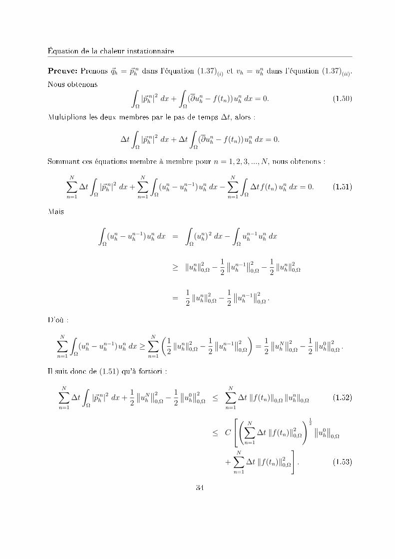
Équation de la chaleur instationnaire
Preuve: Prenons ~qh = ~p nh dans l'équation (1.37)(i) et vh = un
h dans l'équation (1.37)(ii).
Nous obtenons ∫Ω
|~p nh |
2 dx+
∫Ω
(∂unh − f(tn))un
h dx = 0. (1.50)
Multiplions les deux membres par le pas de temps ∆t, alors :
∆t
∫Ω
|~p nh |
2 dx+ ∆t
∫Ω
(∂unh − f(tn))un
h dx = 0.
Sommant ces équations membre à membre pour n = 1, 2, 3, ..., N, nous obtenons :
N∑n=1
∆t
∫Ω
|~p nh |
2 dx+N∑
n=1
∫Ω
(unh − un−1
h )unh dx−
N∑n=1
∫Ω
∆tf(tn)unh dx = 0. (1.51)
Mais ∫Ω
(unh − un−1
h )unh dx =
∫Ω
(unh)2 dx−
∫Ω
un−1h un
h dx
≥ ‖unh‖
20,Ω −
1
2
∥∥un−1h
∥∥2
0,Ω− 1
2‖un
h‖20,Ω
=1
2‖un
h‖20,Ω −
1
2
∥∥un−1h
∥∥2
0,Ω.
D'où :
N∑n=1
∫Ω
(unh − un−1
h )unh dx ≥
N∑n=1
(1
2‖un
h‖20,Ω −
1
2
∥∥un−1h
∥∥2
0,Ω
)=
1
2
∥∥uNh
∥∥2
0,Ω− 1
2
∥∥u0h
∥∥2
0,Ω.
Il suit donc de (1.51) qu'à fortiori :
N∑n=1
∆t
∫Ω
|~p nh |
2 dx+1
2
∥∥uNh
∥∥2
0,Ω− 1
2
∥∥u0h
∥∥2
0,Ω≤
N∑n=1
∆t ‖f(tn)‖0,Ω ‖unh‖0,Ω (1.52)
≤ C
( N∑n=1
∆t ‖f(tn)‖20,Ω
) 12 ∥∥u0
h
∥∥0,Ω
+N∑
n=1
∆t ‖f(tn)‖20,Ω
]. (1.53)
34
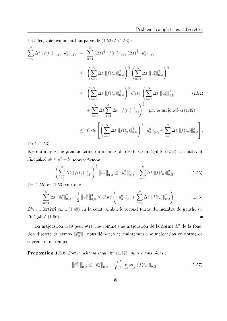
Problème complètement discrétisé
En eet, voici comment l'on passe de (1.52) à (1.53) :N∑
n=1
∆t ‖f(tn)‖0,Ω ‖unh‖0,Ω =
N∑n=1
(∆t)12 ‖f(tn)‖0,Ω (∆t)
12 ‖un
h‖0,Ω
≤
(N∑
n=1
∆t ‖f(tn)‖20,Ω
) 12(
N∑n=1
∆t ‖unh‖
20,Ω
) 12
≤
(N∑
n=1
∆t ‖f(tn)‖20,Ω
) 12
Cste
(N∑
n=1
∆t∥∥u0
h
∥∥2
0,Ω(1.54)
+N∑
n=1
∆tN∑
n=1
∆t ‖f(tn)‖20,Ω
) 12
par la majoration (1.42)
≤ Cste
( N∑n=1
∆t ‖f(tn)‖20,Ω
) 12 ∥∥u0
h
∥∥0,Ω
+N∑
n=1
∆t ‖f(tn)‖20,Ω
.D'où (1.53).
Reste à majorer le premier terme du membre de droite de l'inégalité (1.53). En utilisant
l'inégalité ab ≤ a2 + b2 nous obtenons :(N∑
n=1
∆t ‖f(tn)‖20,Ω
) 12 ∥∥u0
h
∥∥0,Ω
≤∥∥u0
h
∥∥2
0,Ω+
N∑n=1
∆t ‖f(tn)‖20,Ω . (1.55)
De (1.55) et (1.53) suit queN∑
n=1
∆t ‖~p nh ‖
20,Ω +
1
2
∥∥uNh
∥∥2
0,Ω≤ Cste
(∥∥u0h
∥∥2
0,Ω+
N∑n=1
∆t ‖f(tn)‖20,Ω
). (1.56)
D'où à fortiori on a (1.49) en laissant tomber le second terme du membre de gauche de
l'inégalité (1.56) .
La majoration 1.49 peut être vue comme une majoration de la norme L2 de la fonc-
tion discrète du temps ‖~p nh ‖ . nous démontrons maintenant une majoration en norme de
supremum en temps.
Proposition 1.5.6 Soit le schéma implicite (1.37), nous avons alors :∥∥~pNh
∥∥0,Ω
≤∥∥~p 0
h
∥∥0,Ω
+
√T
2max
n=1,...,N‖f(tn)‖0,Ω . (1.57)
35

Équation de la chaleur instationnaire
Preuve: Appliquant l'opérateur de diérence rétrograde ∂ sur (1.37)(i), on trouve :∫Ω
∂~p nh .~qh dx+
∫Ω
∂unh div ~qh dx = 0, ∀~qh ∈ Xh, ∀n ≥ 1. (1.58)
Prenons ~qh = ~p nh dans (1.58), et vh = ∂un
h dans l'équation (1.37)(ii), on obtient le système
suivant : ∫
Ω∂~p n
h . ~pnh dx+
∫Ω∂un
h div ~p nh dx = 0,
∫Ω∂un
h div ~p nh dx+
∫Ωf(tn) ∂un
h dx−∫
Ω
∣∣∂unh
∣∣2 dx = 0.
(1.59)
Soustrayant (1.59)(ii)de (1.59)(i), il s'en suit que :∫Ω
∂~p nh . ~p
nh dx+
∫Ω
∣∣∂unh
∣∣2 =
∫Ω
f(tn) ∂unh dx.
Ceci implique :
‖ ~p nh ‖
20,Ω −
∥∥~p n−1h
∥∥2
0,Ω+ 2∆t
∥∥∂unh
∥∥2 ≤ 2∆t
∫Ω
f(tn) ∂unh dx, (1.60)
Sommant (1.60) membre à membre pour n = 1, 2, 3, ..., N, nous obtenons :
∥∥ ~p Nh
∥∥2
0,Ω−∥∥~p 0
h
∥∥2
0,Ω+
N∑n=1
2∆t∥∥∂un
h
∥∥2 ≤N∑
n=1
2∆t
∫Ω
f(tn) ∂unh dx
≤ 2∆tN∑
n=1
‖f(tn)‖0,Ω
∥∥∂unh
∥∥0,Ω
≤ ∆t
2
N∑n=1
‖f(tn)‖20,Ω + 2∆t
N∑n=1
∥∥∂unh
∥∥2
0,Ω
≤ T
2max
n=1,...,N‖f(tn)‖2
0,Ω + 2∆tN∑
n=1
∥∥∂unh
∥∥2
0,Ω.
D'où : ∥∥ ~p Nh
∥∥0,Ω
≤∥∥~p 0
h
∥∥0,Ω
+
√T
2max
n=1,...,N‖f(tn)‖0,Ω .
36

Problème complètement discrétisé
1.5.3 Estimations d'erreurs
Maintenant nous entamons notre étude sur l'estimation à priori de l'erreur. Nous sup-
posons que f ∈ H1(0, T ;L2(Ω)) et que ∆g+ f(0) ∈ H1(Ω) de sorte que par la proposition
1.4.5 : ut ∈ H1(0, T ;L2(Ω)). En particulier, f et ut sont des fonctions continues de [0, T ]
à valeurs dans L2(Ω). Par une démarche similaire à celle du cas semi-discret, et avant
de donner le résultat sur l'erreur d'approximation de u(t), solution du problème continu
par unh, nous commençons tout d'abord par majorer ‖un
h − uh(tn)‖0,Ω , où (~ph(tn), uh(tn))
∈ Xh × Mh est la solution du problème de projection elliptique à l'instant tn : trouver
(~ph(tn), uh(tn)) ∈ Xh ×Mh solution de∫
Ω~ph(tn).~qh dx+
∫Ωuh(tn) div ~qh dx = 0, ∀~qh ∈ Xh,
∫Ωvh div ~ph(tn)dx = −
∫Ω(f(tn)− ut(tn)) vh dx, ∀vh ∈Mh.
(1.61)
Par soustraction des équations correspondantes de (1.37), on obtient pour les écarts θnh :=
unh − uh(tn) et ~ε n
h := ~p nh − ~ph(tn), le système d'équations aux erreurs :
∫Ω~ε n
h .~qh dx+∫
Ωθn
h div ~qh dx = 0, ∀~qh ∈ Xh,
∫Ωvh div ~ε n
h dx+∫
Ω(ut(tn)− ∂un
h) vh dx = 0, ∀vh ∈Mh.
(1.62)
Théorème 1.5.7 Il existe une constante c > 0 indépendante de h telle que :
‖unh − uh(tn)‖0,Ω ≤ c h
(∫ tn
0
‖ut(s)‖H2,α(Ω) ds
)+ ∆t
∫ tn
0
‖utt(s)‖ ds . (1.63)
Preuve: En remplaçant ~qh par ~ε nh dans (1.62)(i) on obtient :∫
Ω
|~ε nh |
2 +
∫Ω
θnh div ~ε n
h = 0, (1.64)
et aussi en remplaçant vh par θnh dans (1.62)(ii) on a :∫
Ω
θnh div ~εn
h dx+
∫Ω
(ut(tn)− ∂unh) θn
h dx = 0, (1.65)
ce qui implique ∫Ω
|~ε nh |
2 +
∫Ω
(∂uh(tn)− ut(tn)) θnh dx = −
∫Ω
(∂θn
h
)θn
h dx.
37

Équation de la chaleur instationnaire
Lisant cette égalité de droite à gauche, nous obtenons :∫Ω
(θnh)2 dx−
∫Ω
θn−1h θn
h dx = −∆t
∫Ω
|~εnh|
2 −∆t
∫Ω
θnh(∂uh(tn)− ut(tn)) dx
≤ ∆t
∣∣∣∣∫Ω
θnh (∂uh(tn)− ut(tn)) dx
∣∣∣∣≤ ∆t ‖θn
h‖0,Ω
∥∥∂uh(tn)− ut(tn)∥∥
0,Ω.
D'où
‖θnh‖
20,Ω ≤
∫Ω
θn−1h θn
h dx+ ∆t ‖θnh‖0,Ω
∥∥∂uh(tn)− ut(tn)∥∥
0,Ω
≤∥∥θn−1
h
∥∥0,Ω‖θn
h‖0,Ω + ∆t ‖θnh‖∥∥∂uh(tn)− ut(tn)
∥∥0,Ω.
Après simplication des deux membres par ‖θnh‖, on obtient :
‖θnh‖0,Ω ≤
∥∥θn−1h
∥∥0,Ω
+ ∆t∥∥∂uh(tn)− ut(tn)
∥∥0,Ω. (1.66)
Posons pour la suite :
ωn =(∂u(tn)
)∼h− ut(tn) (1.67)
où(∂u(tn)
)∼h
= ∂uh(tn), désigne la projection elliptique de ∂u(tn).
Pour démontrer que(∂u(tn)
)∼h
= ∂uh(tn).
En eet :
Considérons le problème elliptique à l'instant (tj) quelconque :∫
Ω~ph(tj).~qh dx+
∫Ωuh(tj) div ~qh dx = 0, ∀~qh ∈ Xh,
∫Ωvh div ~ph(tj)dx = −
∫Ω(f(tj)− ut(tj)) vh dx, ∀vh ∈Mh.
dénissant la projection elliptique (~ph(tn), uh(tn)).
Ceci implique que pour(~∂ph(tj), ∂uh(tj)
), on aura les équations :
∫Ω~∂ph(tj).~qh dx+
∫Ω∂uh(tj) div ~qh dx = 0, ∀~qh ∈ Xh,
∫Ωvh div
(~∂ph(tj)
)dx = −
∫Ω
(∂f(tj)− ∂ut(tj)
)vh dx, ∀vh ∈Mh.
38
Problème complètement discrétisé
D'autre part on a
∂f(tj)− ∂ut(tj) =f(tj)− f(tj−1)
∆t− ut(tj)− ut(tj−1)
∆t
=(−∆u(tj))− (−∆u(tj−1))
∆t
= −∂∆u(tj) = −∆∂u(tj).
Donc ∫
Ω~∂ph(tj).~qh dx+
∫Ω∂uh(tj) div ~qh dx = 0 ∀~qh ∈ Xh,
∫Ωvh div
(~∂ph(tj)
)dx =
∫Ω
(−∆∂u(tj)
)vh dx ∀vh ∈Mh.
(1.68)
D'où (∂u(tj)
)∼h
= ∂uh(tj). (1.69)
Revenons à (1.67) et posons :
ωn := ωn1 + ωn
2 où
ωn
1 =(∂u(tn)
)∼h− ∂u(tn),
ωn2 = ∂u(tn)− ut(tn) .
(1.70)
Pour ωn1 on a :
‖ωn1 ‖0,Ω =
∥∥(∂u(tn))∼
h− ∂u(tn)
∥∥0,Ω
=∥∥(Rh − I) ∂u(tn)
∥∥0,Ω
=
∥∥∥∥(Rh − I)u(tn)− u(tn−1)
∆t
∥∥∥∥0,Ω
=1
∆t
∥∥∥∥(Rh − I)
∫ tn
tn−1
ut(s) ds
∥∥∥∥0,Ω
≤ 1
∆t
∫ tn
tn−1
‖(Rh − I) ut(s)‖0,Ω ds ≤ 1
∆t
(ch
∫ tn
tn−1
‖ ut(s)‖H2,α(Ω) ds
),
où, par analogie avec le livre de Vidar Thomée [7], Rh de dénote ici la composante dans
Mh du couple de Xh ×Mh projection elliptique de.
39

Équation de la chaleur instationnaire
Donc
∆tn∑
j=1
∥∥ωj1
∥∥0,Ω
≤ chn∑
j=1
(∫ tj
tj−1
‖ ut(s)‖H2,α(Ω) ds
)
≤ ch
∫ tn
t0=0
‖ ut(s)‖H2,α(Ω) ds .
Maintenant, il reste à majorer ωn2 . On a :
‖ωn2 ‖0,Ω =
∥∥∂u(tn)− ut(tn)∥∥
0,Ω
=1
∆t‖u(tn)− u(tn−1)−∆t ut(tn)‖0,Ω
=1
∆t
∥∥∥∥∫ tn
tn−1
(tn−1 − s) utt(s) ds
∥∥∥∥0,Ω
≤∫ tn
tn−1
‖utt(s)‖0,Ω ds.
D'où
∆tn∑
j=1
∥∥ωj2
∥∥0,Ω
≤ ∆t
∫ tn
t0=0
‖utt(s)‖0,Ω ds . (1.71)
Remplaçons dans (1.66), on obtient alors
‖θnh‖0,Ω ≤
∥∥θ0h
∥∥0,Ω
+ ch
∫ tn
t0=0
‖ ut(s)‖H2,α(Ω) ds+ ∆t
∫ tn
t0=0
‖utt(s)‖0,Ω ds. (1.72)
Mais puisque :
θ0h = u0
h − uh(0) = 0,
grâce à l'estimation (40) p.623 de [8].
Alors
‖θnh‖0,Ω ≤ c h
(∫ tn
t0=0
‖ ut(s)‖H2,α(Ω) ds
)+ ∆t
∫ tn
t0=0
‖utt(s)‖0,Ω ds .
Ce qui acheve la démonstration.
Nous sommes maintenant en mesure de donner l'estimation de l'erreur ‖u(tn)− unh‖0,Ω .
40

Problème complètement discrétisé
Théorème 1.5.8 Soit Th une famille régulière de triangulations sur Ω, jouissant des
propriétés (i) et (ii) de la proposition 1.4.6. Pour α ∈]1− π
w, 1[, il existe une constante
c > 0 indépendante de h telle que pour tout n ≥ 1 :
‖u(tn)− unh‖0,Ω ≤ c h
(|u(tn)|H1(Ω) + |u(tn)|H2,α(Ω) +
∫ tn
0
‖ut(s)‖H2,α(Ω) ds
)+∆t
∫ tn
0
‖utt(s)‖ ds . (1.73)
Preuve: Il sut d'appliquer l'inégalité triangulaire :
‖u(tn)− unh‖0,Ω ≤ ‖u(t)− uh(tn)‖0,Ω + ‖uh(tn)− un
h‖0,Ω .
En utilisant l'inégalité (1.63) obtenue précédemment et l'inégalité (1.23) on obtient la
majoration (1.73).
Maintenant nous passons à l'estimation de l'erreur concernant les ~p nh . En suivant une
démarche similaire, nous commençons par démontrer un résultat concernant l'approxi-
mation de ~ph(tn) par ~p nh0,Ω. Pour cela nous adaptons la technique exposée dans [7] p.13,
relative à la formulation classique de l'équation de la chaleur à la méthode mixte duale
pour l'équation de la chaleur.
Proposition 1.5.9
∂‖~ε nh ‖2
0,Ω ≤ 2(~ε n
h , ∂~εnh
). (1.74)
Preuve:
On sait que
∂‖~ε nh ‖2
0,Ω − 2(~ε n
h , ∂~εnh
)=
‖~ε nh ‖2
0,Ω − ‖~ε n−1h ‖2
0,Ω
∆t− 2
(~ε n
h ,~ε n
h − ~ε n−1h
∆t
)
= −‖~ε n
h ‖20,Ω
∆t−‖~ε n−1
h ‖20,Ω
∆t+ 2
(~ε n
h , ~εn−1h
)∆t
=1
∆t
(2(~ε n
h , ~εn−1h
)− ‖~ε n
h ‖20,Ω − ‖~ε n−1
h ‖20,Ω
)
= − 1
∆t
(‖~ε n
h ‖20,Ω + ‖~ε n−1
h ‖20,Ω − 2
(~ε n
h , ~εn−1h
)). (1.75)
41
Équation de la chaleur instationnaire
Mais
2(~ε n
h , ~εn−1h
)≤ 2‖~ε n
h ‖0,Ω ‖~ε n−1h ‖0,Ω ≤ ‖~ε n
h ‖20,Ω + ‖~ε n−1
h ‖20,Ω.
Ce qui implique :
‖~ε nh ‖2
0,Ω + ‖~ε n−1h ‖2
0,Ω − 2(~ε n
h , ~εn−1h
)≥ 0 . (1.76)
De (1.75) et (1.76) suit :
∂‖~ε nh ‖2
0,Ω ≤ 2(~ε n
h , ∂~εnh
).
Proposition 1.5.10
∂‖~ε nh ‖2
0,Ω ≤ ‖ωn‖20,Ω. (1.77)
Preuve:
Par la première équation du système aux erreurs (1.62), il suit :∫Ω
∂~ε nh .~qh dx+
∫Ω
∂θnh div ~qh dx = 0, ∀~qh ∈ Xh .
Prenons ~qh = ~ε nh , d'où :∫
Ω
∂~ε nh .~ε
nh dx = −
∫Ω
(div ~ε nh ) ∂θn
h dx
=
∫Ω
(−ωn − ∂θnh) ∂θn
h dx (d'après (1.62)(ii) et (1.67))
= −∫
Ω
ωn∂θnh dx− ‖∂θn
h‖20,Ω
≤ ‖ωn‖0,Ω ‖∂θnh‖0,Ω − ‖∂θn
h‖20,Ω
≤ 1
2‖ωn‖2
0,Ω +1
2‖∂θn
h‖20,Ω − ‖∂θn
h‖20,Ω
≤ 1
2‖ωn‖2
0,Ω −1
2‖∂θn
h‖20,Ω.
42

Problème complètement discrétisé
En utilisant (1.74) il s'en suit :
∂‖~ε nh ‖2
0,Ω ≤ ‖ωn‖20,Ω − ‖∂θn
h‖20,Ω .
À fortiori
∂‖~ε nh ‖2
0,Ω ≤ ‖ωn‖20,Ω.
Pour pouvoir démarrer les itérations utilisant l'inégalité ∂‖~ε nh ‖2 ≤ ‖ωn‖2 que nous
venons de démontrer, il nous faut majorer ‖~ε 1h ‖ c'est le but de la proposition suivante.
Proposition 1.5.11 Il existe une constante c > 0 indépendante de h telle que :
∥∥~ε 1h
∥∥0,Ω
≤ c h ‖ut‖L2(0,∆t;H2,α(Ω)) + ∆t ‖utt‖L2(0,∆t;L2(Ω)) . (1.78)
Preuve:
Puisque u0h = uh(0) ⇐⇒ θ0
h = 0. Grâce à ce choix de u0h, on a
∂θ1h =
θ1h − θ0
h
∆t=θ1
h
∆t.
Appliquant le système d'équations aux erreurs avec n = 1 nous donne :
∫
Ω~ε 1
h .~qh +∫
Ωθ1
h div ~qh = 0, ∀~qh ∈ Xh,
∫Ωvh div ~ε 1
h −∫
Ω(ω1 + ∂θ1
h) vh = 0, ∀vh ∈Mh.
43
Équation de la chaleur instationnaire
Prenant ~qh = ~ε 1h et vh = θ1
h, nous obtenons :∥∥~ε 1h
∥∥2
0,Ω=
∫Ω
~ε 1h ~ε
1h
= −∫
Ω
θ1h div ~ε 1
h
= −∫
Ω
(ω1 + ∂θ1h) θ
1h
= −∫
Ω
ω1 θ1h −
1
∆t
∫Ω
∣∣θ1h
∣∣2≤ −
∫Ω
ω1 θ1h ≤
∣∣∣∣∫Ω
ω1 θ1h
∣∣∣∣ ≤ ∥∥ω1∥∥
0,Ω
∥∥ θ1h
∥∥0,Ω.
Donc ∥∥~ε 1h
∥∥2
0,Ω≤∥∥ω1
∥∥0,Ω
∥∥ θ1h
∥∥0,Ω
(1.79)
Mais si nous appliquons l'estimée (1.66) avec n = 1, nous obtenons :
∥∥ θ1h
∥∥0,Ω
≡∥∥u1
h − uh(t1)∥∥
0,Ω≤∥∥θ0
h
∥∥0,Ω
+ ∆t∥∥∂uh(t1)− ut(t1)
∥∥0,Ω,
avec θ0h = 0 et ∂uh(t1)− ut(t1) = ω1.
Donc ∥∥ θ1h
∥∥0,Ω
≤ ∆t∥∥ω1
∥∥0,Ω
. (1.80)
Mais (1.79) et (1.80) impliquent
∥∥~ε 1h
∥∥2
0,Ω≤ ∆t
∥∥ω1∥∥2
0,Ω.
Donc
∥∥~ε 1h
∥∥0,Ω
≤√
∆t∥∥ω1
∥∥0,Ω
=√
∆t∥∥∥(∂u(t1))˜h − ut(t1)
∥∥∥0,Ω
≤√
∆t∥∥∥(∂u(t1))˜h − ∂u(t1)
∥∥∥0,Ω
+√
∆t∥∥∂u(t1)− ut(t1)
∥∥0,Ω. (1.81)
44

Problème complètement discrétisé
Et puisque :∥∥∥(∂u(t1))˜h − ∂u(t1)∥∥∥
0,Ω=
∥∥(Rh − I) ∂u(t1)∥∥
0,Ω
=
∥∥∥∥(Rh − I)u(t1)− u0
∆t
∥∥∥∥0,Ω
=1
∆t
∥∥∥∥(Rh − I)
∫ t1=∆t
0
ut(s) ds
∥∥∥∥0,Ω
≤ 1
∆t
∫ ∆t
0
‖(Rh − I) ut(s)‖0,Ω ds
≤ 1
∆t
∫ ∆t
0
ch ‖ut(s)‖H2,α(Ω) ds =ch
∆t
∫ ∆t
0
‖ut(s)‖H2,α(Ω) ds
par (40) p.623 de [8]
≤ ch
∆t
√∆t
(∫ ∆t
0
‖ut(s)‖2H2,α(Ω) ds
) 12
=ch√∆t
‖ut(·)‖L2(0,∆t;H2,α(Ω)) .
D'où√
∆t∥∥∥(∂u(t1))˜h − ∂u(t1)
∥∥∥0,Ω
≤ c h ‖ut(·)‖L2(0,∆t;H2,α(Ω)) . (1.82)
D'autre part
∥∥∂u(t1)− ut(t1)∥∥
0,Ω=
∥∥∥∥u(t1)− u(t0)
∆t− ut(t1)
∥∥∥∥0,Ω
=1
∆t‖u(t1)− u(t0)−∆tut(t1)‖0,Ω .
Mais par la formule de Taylor avec reste intégral :
u(t0) = u(t1)−∆tut(t1) +
∫ t0=0
t1=∆t
utt(s)(t0 − s)ds
= u(t1)−∆tut(t1) +
∫ t1
0
utt(s)sds
u(t1)− u(t0)−∆tut(t1) = −∫ t1
0
utt(s)sds.
45

Équation de la chaleur instationnaire
D'où
∥∥∂u(t1)− ut(t1)∥∥
0,Ω≤ 1
∆t
∫ t1
0
‖utt(s)‖0,Ω sds
≤ 1
∆t
(∫ t1
0
‖utt(s)‖20,Ω ds
) 12(∫ t1
0
s2ds
) 12
≤ 1
∆t
(∆t3
3
) 12
‖utt(·)‖L2(0,∆t;L2(Ω))
≤√
∆t ‖utt(s)‖L2(0,∆t;L2(Ω)) .
Donc√
∆t∥∥∂u(t1)− ut(t1)
∥∥0,Ω
≤ ∆t ‖utt(s)‖L2(0,∆t;L2(Ω)) . (1.83)
De (1.81),(1.82) et (1.83) suit :
∥∥~ε 1h
∥∥0,Ω
≤ c h ‖ut‖L2(0,∆t;H2,α(Ω)) + ∆t ‖utt‖L2(0,∆t;L2(Ω)).
Nous pouvons maintenant démontrer l'estimée de ‖~ε nh ‖0,Ω.
Théorème 1.5.12 Il existe une constante c > 0 indépendante de h telle que :
‖~ε nh ‖0,Ω ≤ c
(h ‖ut‖L2(0,tn;H2,α(Ω)) + ∆t ‖utt‖L2(0,tn;L2(Ω))
)(1.84)
Preuve:
Appliquons récursivement l'inégalité ∂ ‖~ε nh ‖
20,Ω ≤ ‖ωn‖2
0,Ω. On a donc :
‖~ε 2h ‖
2 − ‖~ε 1h ‖
2 ≤ ∆t ‖ω2‖2
‖~ε 3h ‖
2 − ‖~ε2h‖
2 ≤ ∆t ‖ω3‖2
...
...
‖~ε nh ‖
2 −∥∥~ε n−1
h
∥∥2 ≤ ∆t ‖ωn‖2 .
46

Problème complètement discrétisé
Sommant ces inégalités membre à membre, nous obtenons :
‖~ε nh ‖
20,Ω −
∥∥~ε 1h
∥∥2
0,Ω≤ ∆t
(∥∥ω2∥∥2
0,Ω+ · · ·+ ‖ωn‖2
0,Ω
).
Donc
‖~ε nh ‖
20,Ω ≤
∥∥~ε 1h
∥∥2
0,Ω+ ∆t
j=n∑j=2
∥∥ωj∥∥2
0,Ω. (1.85)
En utilisant le fait que ωj = ωj1 + ωj
2 où ωj1et ω
j2 ont été dénis en (1.70) , on a
∆t
j=n∑j=2
∥∥ωj∥∥2
0,Ω≤ 2∆t
j=n∑j=2
∥∥ωj1
∥∥2
0,Ω+ 2∆t
j=n∑j=2
∥∥ωj2
∥∥2
0,Ω.
Comme
ωj1 = (Rh − I) ∂u(tj) =
1
∆t(Rh − I)
∫ tj
tj−1
ut(s)ds
=1
∆t
∫ tj
tj−1
(Rh − I) ut(s)ds,
et donc
∥∥ωj1
∥∥0,Ω
≤ 1
∆t
∫ tj
tj−1
‖(Rh − I) ut(s)‖0,Ω ds
≤ h
∆t
∫ tj
tj−1
‖ut(s)‖H2,α(Ω) ds.
Ceci entraîne
∆t
j=n∑j=2
∥∥ωj1
∥∥2
0,Ω≤ ∆t
h2
∆t2
j=n∑j=2
(∫ tj
tj−1
‖ut(s)‖H2,α(Ω) ds
)2
≤ ∆th2
∆t
j=n∑j=2
∫ tj
tj−1
‖ut(s)‖2H2,α(Ω) ds
= h2
∫ tn
t1
‖ut(s)‖2H2,α(Ω) ds .
47

Équation de la chaleur instationnaire
Pour les ωj2 on a
∆t
j=n∑j=2
∥∥ωj2
∥∥2
0,Ω= ∆t
j=n∑j=2
∥∥∂u(tj)− ut(tj)∥∥2
0,Ω
=1
∆t
j=n∑j=2
‖u(tj)− u(tj−1)−∆tut(tj)‖20,Ω .
Par la formule de Taylor avec reste intégral, on obtient :
u(tj−1) = u(tj) + ut(tj)(tj−1 − tj) +
∫ tj−1
tj
utt(s)(tj−1 − s)ds.
D'où
‖u(tj)− u(tj−1)−∆tut(tj)‖20,Ω =
∥∥∥∥∥∫ tj−1
tj
utt(s)(tj−1 − s)ds
∥∥∥∥∥2
0,Ω
≤
(∫ tj
tj−1
‖utt(s)‖0,Ω |(tj−1 − s) | ds
)2
≤
(∫ tj
tj−1
‖utt(s)‖20,Ω ds
)∆t3
3.
Alors
∆t
j=n∑j=2
∥∥ωj2
∥∥2 ≤ ∆t2
3
∫ tn
t1
‖utt(s)‖20,Ω ds.
D'où :
∆t
j=n∑j=2
∥∥ωj∥∥2
0,Ω≤ 2∆t
j=n∑j=2
∥∥ωj1
∥∥2
0,Ω+ 2∆t
j=n∑j=2
∥∥ωj2
∥∥2
0,Ω
≤ 2h2
∫ tn
t1
‖ut(s)‖2H2,α(Ω) ds+ ∆t2
(∫ tn
t1
‖utt(s)‖20,Ω ds
).
De (1.85) suit alors
‖~ε nh ‖
20,Ω ≤
∥∥~ε 1h
∥∥2
0,Ω+ ∆t
j=n∑j=2
∥∥ωj∥∥2
0,Ω
≤ ch2
∫ tn
t0=0
‖ut(s)‖2H2,α(Ω) ds+ 2∆t2
∫ tn
t0=0
‖utt(s)‖20,Ω ds,
48

Problème complètement discrétisé
par la proposition précédente.
Donc on a bien
‖~ε nh ‖0,Ω ≤ c
(h ‖ut‖L2(0,tn;H2,α(Ω)) + ∆t ‖utt‖L2(0,tn;L2(Ω))
).
Et pour terminer on sait déjà par la proposition 1.4.6 que
∥∥∥~p(t)− ~ph(t)∥∥∥
0,Ω≤ c h |u(t)|H2,α(Ω) ,∀
′t ∈ I.
En vertu de l'inégalité 1.84 il sut donc d'appliquer l'inégalité triangulaire pour majorer
‖~p(tn)− ~p nh ‖0,Ω, ∀n ≥ 1. En conclusion, nous avons établi le théorème :
Théorème 1.5.13 Soit Th une famille régulière de triangulations sur Ω, jouissant des
propriétés (i) et (ii) de la proposition (1.4.6). Pour α ∈]1− π
w, 1[, il existe une constante c >
0 indépendante de h et de ∆t telle que pour tout n ≥ 1 :
‖~p(tn)− ~p nh ‖0,Ω ≤ c
(h(|u(tn)|H2,α(Ω) + ‖ut‖L2(0,tn;H2,α(Ω))
)+ ∆t ‖utt‖L2(0,tn;L2(Ω))
).
(1.86)
Toujours dans notre étude du problème complètement discrétisé de l'équation de la
chaleur, nous allons développer une autre méthode de schéma implicite. Il s'agit du schéma
de Crank-Nicolson, adapté à la méthode mixte.
1.5.4 Schéma de Crank-Nicolson
Avant de donner la formulation mixte complètement discrétisée par le schéma de Crank-
Nicolson, nous allons tout d'abord dénir de nouvelles variables. On pose :
tn− 12
=tn + tn−1
2, ~p
n− 12
h =~p n
h + ~p n−1h
2, et u
n− 12
h =un
h + un−1h
2. (1.87)
49

Équation de la chaleur instationnaire
Considérons alors le problème suivant :
∫Ω~p
n− 12
h .~qh dx+∫
Ωu
n− 12
h div ~qh dx = 0, ∀~qh ∈ Xh, ∀n ≥ 1
∫Ωvh div ~p
n− 12
h dx = −∫
Ω(f(tn− 1
2)− ∂un
h) vh dx, ∀vh ∈Mh, ∀n ≥ 1
u0h (c.i.), donnée.
(1.88)
Remarquons que dans (1.88) apparaît ~pn− 1
2h , u
n− 12
h , unh et un−1
h . On peux donc choisir comme
inconnues les ~pn− 1
2h , un
h pour n ≥ 1. Une autre alternative est de considérer que les inconnues
sont les ~p nh pour n ≥ 0 et un
h pour n ≥ 1. u0h étant la condition initiale est connu et ~p 0
h est
déni exceptionnellement par l'équation
∫Ω
~p 0h .~qh dx+
∫Ω
u0h div ~qh dx = 0, ∀~qh ∈ Xh. (1.89)
Ce dernier choix des inconnues présente les avantages suivants :
inconnues traditionnelles.
symétrie en ~p et en u du problème.
Proposition 1.5.14 Le problème (1.88) admet une et une seule solution (~p nh , u
nh)n∈N ∈
Xh ×Mh.
Preuve: Commençons par démontrer l'unicité. Pour cela, montrons que si (~p nh , u
nh) ∈
Xh ×Mh vérie
∫Ω~p
n− 12
h .~qh dx+∫
Ωu
n− 12
h div ~qh dx = 0, ∀~qh ∈ Xh, ∀n ≥ 1
∫Ωvh div ~p
n− 12
h dx =∫
Ω∂un
h vh dx, ∀vh ∈Mh, ∀n ≥ 1
u0h = 0,
(1.90)
alors (~p nh , u
nh) = 0.
En prenant ~qh = ~pn− 1
2h dans la première équation de (1.90) et vh = u
n− 12
h dans la deuxième
équation de (1.90) , on obtient∫Ω
∣∣∣~p n− 12
h
∣∣∣2 dx+
∫Ω
∂unh u
n− 12
h dx = 0. (1.91)
50

Problème complètement discrétisé
D'autre part, on a
∂unh u
n− 12
h =1
2∆t
(un
h − un−1h
) (un
h + un−1h
)=
1
2∆t(un
h)2 , (1.92)
à condition d'avoir déjà démontré que un−1h = 0. Prenons alors n = 1 dans (1.92) et puisque
u0h = 0 (condition initiale), par conséquent u1
h = 0, et ainsi pour n = 2, 3, .... D'autre part,
d'après (1.89) , u0h = 0 implique ~p 0
h = 0. Et comme on sait déjà que ~p12
h = 0, par (1.91) avec
n = 1, il s'en suit que ~p 1h = 0. Donc ~p 2
h = 0 par (1.91) avec n = 2 et ainsi de suite pour
tout n ≥ 1.
Pour l'existence, on sait par le théorème de représentation de Riez que ~p 0h existe (Cf.
remarque (1.5.2)).On considère ensuite le système (1.88) avec n = 1, avec comme but de
construire ~p 1h et u1
h sachant que u0h et ~p 0
h sont connus. On a
∫Ω~p 1
h .~qh dx+∫
Ωu1
h div ~qh dx =∫
Ω~p 0
h .~qh dx+∫
Ωu0
h div ~qh dx, ∀~qh ∈ Xh,
∫Ωvh div ~p 1
h dx− 2∆t
∫Ωu1
h vh dx = −∫
Ωvh div ~p 0
h dx− 2∆t
∫Ωu0
h vh dx− 2∫
Ωf(t1/2
)vh dx,
∀vh ∈Mh.
(1.93)
Considérons donc l'application Φh de Xh ×Mh dans son dual X ′h ×M ′
h, dénie par :(~p 1
h , u1h
)7−→
(~qh 7−→
∫Ω
~p 1h .~qh dx+
∫Ω
u1h div ~qh dx,
vh 7−→∫
Ω
vh div ~p 1h dx−
2
∆t
∫Ω
u1h vh dx
).
Donc tout revient à démontrer que c'est un isomorphisme. Puisque Φh est linéaire de
Xh × Mh dans son dual, et que les deux espaces Xh × Mh et X ′h × M ′
h ont la même
dimension, il sut de montrer que Φh est injective pour démontrer sa bijectivité. Soit
(~p 1h , u
1h) tel que : ∫
Ω
~p 1h .~qh dx+
∫Ω
u1h div ~qh dx = 0, ∀~qh ∈ Xh (1.94)∫
Ω
vh div ~p 1h dx−
2
∆t
∫Ω
u1h vh dx = 0, ∀vh ∈Mh. (1.95)
Dans (1.94) , prenons ~qh = ~p 1h et vh = u1
h dans (1.95) , il s'en suit que :∫Ω
∣∣~p 1h
∣∣2 dx+2
∆t
∫Ω
∣∣u1h
∣∣2 dx = 0. (1.96)
51

Équation de la chaleur instationnaire
On obtient ~p 1h = 0 et u1
h = 0. D'où l'injectivité et donc la bijectivité de Φh.
Il sut alors, d'appliquer Φ−1h au couple de formes linéaires dénies par les deux membres
de droite des deux équations du système (1.93) .
De manière similaire on construit ensuite (~p 2h , u
2h) en considérant le système (1.88) , avec
n = 2 et ainsi de suite.
1.5.5 Stabilité du schéma de Crank-Nicolson
Maintenant on va démontrer le résultat de stabilité du Schéma Crank-Nicolson.
Théorème 1.5.15 Supposons ∆t ≤ 12, il existe une constante c > 0 indépendante de h
telle que : ∥∥uNh
∥∥0,Ω.∥∥u0
h
∥∥0,Ω
+√
∆t∥∥~p 0
h
∥∥0,Ω
+
√√√√ N∑n=1
∆t∥∥∥f(tn− 1
2)∥∥∥2
0,Ω
Preuve: Considérons alors le problème suivant :∫
Ω~p n
h .~qh dx+∫
Ωun
h div ~qh dx = 0, ∀~qh ∈ Xh, ∀n ≥ 1
∫Ωvh div ~p
n− 12
h dx = −∫
Ω(f(tn− 1
2)− ∂un
h) vh dx, ∀vh ∈Mh, ∀n ≥ 1
(1.97)
Prenons vh = unh dans la deuxième équation. On obtient :∫
Ω
unh div
(~p n
h + ~p n−1h
2
)dx = −
∫Ω
(f(tn− 12)− ∂un
h) unh dx
=1
∆t
∫Ω
(un
h − un−1h
)un
h dx−∫
Ω
f(tn− 12)un
h dx.(1.98)
Par la première équation de (1.97) , on a :∫Ω
unh div ~p n
h dx = −∫
Ω
|~p nh |
2 dx, (1.99)
et : ∫Ω
unh div ~p n−1
h dx = −∫
Ω
~p n · ~p n−1h dx. (1.100)
52

Problème complètement discrétisé
De (1.98), (1.99) et (1.100) , nous obtenons
1
2
∫Ω
|~p nh |
2 dx+1
2
∫Ω
~p n · ~p n−1h dx+
1
∆t
∫Ω
|unh|
2 dx− 1
∆t
∫Ω
un−1h un
hdx =
∫Ω
f(tn− 12)un
hdx.
Donc
1
∆t
∫Ω
|unh|
2 dx+1
2
∫Ω
|~p nh |
2 dx = −1
2
∫Ω
~p nh · ~p n−1
h dx+1
∆t
∫Ω
un−1h un
hdx+
∫Ω
f(tn− 12)un
hdx,
d'où :
1
2∆t
∫Ω
|unh|
2 dx+1
4∆t
∫Ω
|~p nh |
2 dx ≤ 1
4
∫Ω
∣∣~p n−1h
∣∣2 dx+1
2∆t
∫Ω
∣∣un−1h
∣∣2 dx+
1
2
∫Ω
∣∣∣f(tn− 12)∣∣∣2 dx+
1
2
∫Ω
|unh|
2 dx.
On obtient :
‖unh‖
20,Ω +
∆t
2‖~p n
h ‖20,Ω ≤
∆t
2
∥∥~p n−1h
∥∥2
0,Ω+∥∥un−1
h
∥∥2
0,Ω+ ∆t ‖un
h‖20,Ω + ∆t
∥∥∥f(tn− 12)∥∥∥2
0,Ω.
Autrement, on a :
‖unh‖
20,Ω −
∥∥un−1h
∥∥2
0,Ω+
∆t
2
(‖~p n
h ‖20,Ω −
∥∥~p n−1h
∥∥2
0,Ω
)≤ ∆t ‖un
h‖20,Ω + ∆t
∥∥∥f(tn− 12)∥∥∥2
0,Ω.
Et alors
N∑n=1
(‖un
h‖20,Ω −
∥∥un−1h
∥∥2
0,Ω
)+
∆t
2
N∑n=1
(‖~p n
h ‖20,Ω −
∥∥~p n−1h
∥∥2
0,Ω
)≤ ∆t
N∑n=1
‖unh‖
20,Ω
+∆tN∑
n=1
∥∥∥f(tn− 12)∥∥∥2
0,Ω.
Donc :
∥∥uNh
∥∥2
0,Ω+
∆t
2
∥∥~pNh
∥∥2
0,Ω≤∥∥u0
h
∥∥2
0,Ω+
∆t
2
∥∥~p 0h
∥∥2
0,Ω+ ∆t
N∑n=1
‖unh‖
20,Ω + ∆t
N∑n=1
∥∥∥f(tn− 12)∥∥∥2
0,Ω.
En vue d'appliquer l'inégalité de Gronwall discrète, faisons passer le terme ∆t∥∥uN
h
∥∥2
0,Ωdu
membre de droite au membre de gauche. On obtient :
(1−∆t)∥∥uN
h
∥∥2
0,Ω+
∆t
2
∥∥~pNh
∥∥2
0,Ω≤∥∥u0
h
∥∥2
0,Ω+
∆t
2
∥∥~p 0h
∥∥2
0,Ω+∆t
N∑n=1
‖unh‖
20,Ω+∆t
N∑n=1
∥∥∥f(tn− 12)∥∥∥2
0,Ω.
53

Équation de la chaleur instationnaire
Supposons ∆t ≤ 12, on a :
∥∥uNh
∥∥2
0,Ω+∆t
∥∥~pNh
∥∥2
0,Ω≤ 2
∥∥u0h
∥∥2
0,Ω+∆t
∥∥~p 0h
∥∥2
0,Ω+2∆t
N∑n=1
‖unh‖
20,Ω +2∆t
N∑n=1
∥∥∥f(tn− 12)∥∥∥2
0,Ω.
Par l'inégalité de Gronwall discrète ([19] p.VI-9), avec :
ϕn = ‖unh‖
20,Ω + ∆t ‖~p n
h ‖20,Ω
m0 = 2
m1 = · · · = mN−1 = 2∆t
C = 2 ‖u0h‖
20,Ω + ∆t ‖~p 0
h ‖20,Ω + 2∆t
∑Nn=1
∥∥∥f(tn− 12)∥∥∥2
0,Ω,
on obtient ∥∥uNh
∥∥2
0,Ω+ ∆t
∥∥~pNh
∥∥2
0,Ω
≤
(2∥∥u0
h
∥∥2
0,Ω+ ∆t
∥∥~p 0h
∥∥2
0,Ω+ 2∆t
N∑n=1
∥∥∥f(tn− 12)∥∥∥2
0,Ω
)exp
(N−1∑∆t=0
m∆t
)
=
(2∥∥u0
h
∥∥2
0,Ω+ ∆t
∥∥~p 0h
∥∥2
0,Ω+ 2∆t
N∑n=1
∥∥∥f(tn− 12)∥∥∥2
0,Ω
)exp (2 + 2 (N − 1) ∆t) .
En particulier :
∥∥uNh
∥∥2
0,Ω+∆t
∥∥~pNh
∥∥2
0,Ω≤ exp(2)
(2∥∥u0
h
∥∥2
0,Ω+ ∆t
∥∥~p 0h
∥∥2
0,Ω+ 2∆t
N∑n=1
∥∥∥f(tn− 12)∥∥∥2
0,Ω
)(exp(T ))2 .
Et alors : ∥∥uNh
∥∥2
0,Ω+ ∆t
∥∥~pNh
∥∥2
0,Ω.∥∥u0
h
∥∥2
0,Ω+ ∆t
∥∥~p 0h
∥∥2
0,Ω+
N∑n=1
∆t∥∥∥f(tn− 1
2)∥∥∥2
0,Ω,
Donc on a ∥∥uNh
∥∥2
0,Ω.∥∥u0
h
∥∥2
0,Ω+ ∆t
∥∥~p 0h
∥∥2
0,Ω+
N∑n=1
∆t∥∥∥f(tn− 1
2)∥∥∥2
0,Ω.
Proposition 1.5.16 Soit le schéma implicite (1.37), nous avons alors :
∥∥~pNh
∥∥0,Ω
≤∥∥~p 0
h
∥∥0,Ω
+
√T
2max
n=1,...,N‖f(tn)‖0,Ω . (1.101)
54

Problème complètement discrétisé
Preuve: Appliquant l'opérateur de diérence rétrograde ∂ sur (1.97)(i), on trouve :∫Ω
∂~p nh .~qh dx+
∫Ω
∂unh div ~qh dx = 0, ∀~qh ∈ Xh, ∀n ≥ 1. (1.102)
Prenons ~qh = ~pn− 1
2h dans (1.102), et vh = ∂un
h dans l'équation (1.97)(ii), on obtient le
système suivant :∫
Ω∂~p n
h . ~pn− 1
2h dx+
∫Ω∂un
h div ~pn− 1
2h dx = 0,
∫Ω∂un
h div ~pn− 1
2h dx+
∫Ωf(tn) ∂un
h dx−∫
Ω
∣∣∂unh
∣∣2 dx = 0.
(1.103)
Soustrayant (1.103)(ii)de (1.103)(i), il s'en suit que :∫Ω
∂~p nh . ~p
n− 12
h dx+
∫Ω
∣∣∂unh
∣∣2 =
∫Ω
f(tn) ∂unh dx.
Nous avons donc :∫Ω
(~p n
h − ~p n−1h
∆t
).
(~p n
h + ~p n−1h
2
)dx+
∫Ω
∣∣∂unh
∣∣2 =
∫Ω
f(tn) ∂unh dx,
et alors :
‖ ~p nh ‖
20,Ω −
∥∥~p n−1h
∥∥2
0,Ω+ 2∆t
∥∥∂unh
∥∥2= 2∆t
∫Ω
f(tn) ∂unh dx. (1.104)
Sommant (1.104) membre à membre pour n = 1, 2, 3, ..., N, nous obtenons :
∥∥ ~p Nh
∥∥2
0,Ω−∥∥~p 0
h
∥∥2
0,Ω+
N∑n=1
2∆t∥∥∂un
h
∥∥2=
N∑n=1
2∆t
∫Ω
f(tn) ∂unh dx
≤ 2∆tN∑
n=1
‖f(tn)‖0,Ω
∥∥∂unh
∥∥0,Ω
≤ ∆t
2
N∑n=1
‖f(tn)‖20,Ω + 2∆t
N∑n=1
∥∥∂unh
∥∥2
0,Ω
≤ T
2max
n=1,...,N‖f(tn)‖2
0,Ω + 2∆tN∑
n=1
∥∥∂unh
∥∥2
0,Ω.
D'où : ∥∥ ~p Nh
∥∥0,Ω
≤∥∥~p 0
h
∥∥0,Ω
+
√T
2max
n=1,...,N‖f(tn)‖0,Ω .
55

Équation de la chaleur instationnaire
1.5.6 Estimations d'erreurs
Pour démontrer les résultats d'estimées d'erreurs, on utilisera une démarche analogue
à celle employée pour le schéma précédent. Le problème elliptique (1.61) étant vrai pour
n et n− 1, en faisant la somme nous obtenons :∫
Ω
~ph(tn)+~ph(tn−1)2
.~qh dx+∫
Ωuh(tn)+uh(tn−1)
2div ~qh dx = 0, ∀~qh ∈ Xh,
∫Ωvh div
~ph(tn)+~ph(tn−1)2
dx = −∫
Ω(f(tn)+f(tn−1)
2− ut(tn)+ut(tn−1)
2) vh dx, ∀vh ∈Mh.
(1.105)
Réécrivant le schéma de Crank-Nicolson :
∫Ω~p
n− 12
h .~qh dx+∫
Ωu
n− 12
h div ~qh dx = 0, ∀~qh ∈ Xh, ∀n ≥ 1
∫Ωvh div ~p
n− 12
h dx = −∫
Ω(f(tn− 1
2)− ∂un
h) vh dx, ∀vh ∈Mh, ∀n ≥ 1
u0h (c.i.), donnée.
(1.106)
Notons les écarts θnh := un
h − uh(tn) et ~ε nh := ~p n
h − ~ph(tn). Par soustraction on obtient le
système d'équations aux erreurs :
∫Ω
~ε nh +~ε n−1
h
2.~qh dx+
∫Ω
θnh+θn−1
h
2div ~qh dx = 0, ∀~qh ∈ Xh,
∫Ωvh div
~ε nh +~ε n−1
h
2dx = −
∫Ω(f(tn− 1
2)− f(tn)+f(tn−1)
2−(∂un
h −ut(tn)+ut(tn−1)
2
)) vh dx,
∀vh ∈Mh.
(1.107)
Proposition 1.5.17 Supposons que f, dfdt∈ H1(0, T ;L2(Ω)), ∆g + f(0) ∈ H1(Ω) et aussi
∆ (∆g + f(0)) + dfdt
(0) ∈ H1 (Ω) . Alors
uttt ∈ L2(0, T ;L2(Ω))
Preuve: Soit w ∈ H1(0, T ;L2(Ω)) ∩ L2(0, T ;L2(Ω)) la solution de l'équation de diusion
de la chaleur dwdt
(t) = ∆w(t) + d2fdt2
(t), ∀′t ∈ [0, T ]
w(0) = ∆ (∆g + f(0)) + dfdt
(0).
56

Problème complètement discrétisé
Posons v(t) =∫ t
0w(s) ds+ ∆g + f(0), dv
dt(t) = w(t) et v(0) = ∆g + f(0) ∈ H1(Ω).
Intégrant l'équation dwdt
(s) = ∆w(s) + d2fdt
(s), ∀′s ∈ [0, T ] de 0 à t, nous obtenons :
w(t)− w(0) = ∆ (v(t)−∆g − f(0)) +df
dt(t)− df
dt(0)
i.e.dv
dt(t)−∆ (∆g + f(0))− df
dt(0) = ∆v(t)−∆ (∆g + f(0)) +
df
dt(t)− df
dt(0).
Simpliant les 2 membres nous obtenons que v est la solution du problème de Cauchy : dvdt
(t) = ∆v(t) + d2fdt2
(t)
v(0) = ∆g + f(0) ∈ H1(Ω).
Mais nous avons vu dans la preuve de la démonstration de la proposition 1.4.5 que v = dudt.
Donc d2udt2
= dvdt
= w ∈ H2(0, T ;L2(Ω)). D'où
uttt ∈ L2(0, T ;L2(Ω)).
Maintenant on va démontrer le résultat de majoration de ‖unh − uh(tn)‖0,Ω .
Théorème 1.5.18 Sous les hypothèses de la proposition précédente il existe une constante
c > 0 indépendante de h et de k telle que :
‖unh − uh(tn)‖0,Ω ≤ ch
(‖u0‖H2,α(Ω) +
∫ tn
0
‖ut(s)‖H2,α(Ω) ds
)+
(1.108)
2∆t2(∫ tn
0
‖uttt(s)‖0,Ω ds+
∫ tn
0
‖ftt(s)‖0,Ω ds
).
Preuve: La première étape de cette démonstration est de majorer ‖θnh‖ en fonction de∥∥θn−1
h
∥∥0,Ω
et de ‖ωn‖0,Ω . Pour cela prenons vh = θnh + θn−1
h dans la deuxième équation du
système (1.107) et ~qh = ~ε nh + ~ε n−1
h dans la première, on a donc :∫Ω
∣∣~ε nh + ~ε n−1
h
∣∣22
dx (1.109)
=
∫Ω
(f(tn− 1
2)− f(tn) + f(tn−1)
2−(∂un
h −ut(tn) + ut(tn−1)
2
)) (θn
h + θn−1h
)dx.
57

Équation de la chaleur instationnaire
Regardons de plus près le terme ∂unh −
ut(tn)+ut(tn−1)2
; on a :
∂unh −
ut(tn) + ut(tn−1)
2= ∂θn
h + u(tn)− u(tn−1)−ut(tn) + ut(tn−1)
2
= ∂θnh + (Rh − I) ∂u(tn) + ∂u(tn)− ut(tn) + ut(tn−1)
2.
Et donc
∂unh −
ut(tn) + ut(tn−1)
2+f(tn) + f(tn−1)
2− f(tn− 1
2)
= ∂θnh + (Rh − I) ∂u(tn) +
(∂u(tn)− ut(tn− 1
2))
+ ut(tn− 12)− ut(tn) + ut(tn−1)
2
+f(tn) + f(tn−1)
2− f(tn− 1
2) (1.110)
= ∂θnh + (Rh − I) ∂u(tn) +
(∂u(tn)− ut(tn− 1
2))
+ ∆
[u(tn− 1
2)− 1
2(u(tn) + u(tn−1))
].
puisque ∆u(t) + f(t) = ut(t), pour tout t > 0.
Posons pour la suite ωn := ωn1 + ωn
2 + ωn3 , avec :
ωn1 : = (Rh − I) ∂u(tn),
ωn2 : =
(∂u(tn)− ut(tn− 1
2)),
ωn3 : = ∆
[u(tn− 1
2)− 1
2(u(tn) + u(tn−1))
].
De (1.110) et (1.109), suit que∫Ω
∣∣~ε nh + ~ε n−1
h
∣∣22
dx = −∫
Ω
(∂θnh + ωn)
(θn
h + θn−1h
)dx. (1.111)
On obtient donc∫Ω
∂θnh
(θn
h + θn−1h
)dx ≤ −1
2
∥∥~ε nh + ~ε n−1
h
∥∥2+ ‖ωn‖
∥∥θnh + θn−1
h
∥∥ .Mais ∫
Ω
∂θnh
(θn
h + θn−1h
)dx =
‖θnh‖
2 −∥∥θn−1
h
∥∥2
∆t. (1.112)
58

Problème complètement discrétisé
Alors :
‖θnh‖
20,Ω −
∥∥θn−1h
∥∥2
0,Ω≤ ∆t
(−1
2
∥∥~ε nh + ~ε n−1
h
∥∥2
0,Ω+ ‖ωn‖0,Ω
∥∥θnh + θn−1
h
∥∥0,Ω
). (1.113)
D'où à fortiori (1.114) , en laissant tomber le premier terme du membre de gauche de
l'inégalité (1.113), nous obtenons
‖θnh‖
2 −∥∥θn−1
h
∥∥2 ≤ ∆t ‖ωn‖0,Ω
(‖θn
h‖0,Ω +∥∥θn−1
h
∥∥0,Ω
). (1.114)
Donc :
‖θnh‖0,Ω ≤
∥∥θn−1h
∥∥0,Ω
+ ∆t ‖ωn‖0,Ω , (1.115)
il sut alors de majorer ωn. Commençons par ωn2 . Par dénition on a :
∆t ‖ωn2 ‖0,Ω = ∆t
∥∥∥∂u(tn)− ut(tn− 12)∥∥∥
0,Ω
= ∆t
∥∥∥∥u(tn)− u(tn−1)
∆t− ut(tn− 1
2)
∥∥∥∥0,Ω
=∥∥∥u(tn)− u(tn−1)−∆t ut(tn− 1
2)∥∥∥
0,Ω.
Par la formule de Taylor on a :
u(tn) = u(tn− 12) +
∆t
2ut(tn− 1
2) +
∆t2
8utt(tn− 1
2) +
1
2
∫ tn
tn− 1
2
(tn − s)2uttt(s)ds,
et à l'instant tn−1 :
u(tn−1) = u(tn− 12)− ∆t
2ut(tn− 1
2) +
∆t2
8utt(tn− 1
2) +
1
2
∫ tn−1
tn− 1
2
(tn−1 − s)2uttt(s)ds. (1.116)
Considérons la diérence de ces deux égalités. Nous obtenons :
u(tn)− u(tn−1)−∆t ut(tn− 12) =
1
2
∫ tn
tn− 1
2
(tn − s)2uttt(s)ds−1
2
∫ tn−1
tn− 1
2
(tn−1 − s)2uttt(s)ds.
59

Équation de la chaleur instationnaire
D'où ∥∥∥u(tn)− u(tn−1)−∆t ut(tn− 12)∥∥∥
0,Ω
≤ 1
2
∫ tn
tn− 1
2
(tn − s)2 ‖uttt(s)‖0,Ω ds+1
2
∫ tn−1
tn− 1
2
(tn−1 − s)2 ‖uttt(s)‖0,Ω ds
≤ ∆t2
8
∫ tn
tn− 1
2
‖uttt(s)‖0,Ω ds+∆t2
8
∫ tn− 1
2
t−1
‖uttt(s)‖0,Ω ds
=∆t2
8
∫ tn
tn−1
‖uttt(s)‖0,Ω ds.
Nous avons donc démontré que
∆t ‖ωn2 ‖0,Ω ≤
∆t2
8
∫ tn
tn−1
‖uttt(s)‖0,Ω ds. (1.117)
Maintenant cherchons à majorer ‖ωn3 ‖0,Ω. La formule de Taylor nous donne
1
2u(tn) =
1
2u(tn− 1
2) +
∆t
4ut(tn− 1
2) +
1
2
∫ tn
tn− 1
2
(tn − s)utt(s)ds,
1
2u(tn−1) =
1
2u(tn− 1
2)− ∆t
4ut(tn− 1
2) +
1
2
∫ tn−1
tn− 1
2
(tn − s)utt(s)ds.
En faisant la somme de ces deux égalités nous obtenons :
u(tn− 12)− 1
2(u(tn) + u(tn−1)) = −1
2
∫ tn
tn− 1
2
(tn − s)utt(s)ds−1
2
∫ tn−1
tn− 1
2
(tn−1 − s)utt(s)ds.
Appliquant alors l'opérateur laplacien ∆, nous obtenons :∥∥∥∥∆ [u(tn− 12)− 1
2(u(tn) + u(tn−1))
]∥∥∥∥0,Ω
≤ 1
2
∫ tn
tn− 1
2
(tn − s) ‖∆utt(s)‖0,Ω ds+1
2
∫ tn− 1
2
tn−1
|tn−1 − s| ‖∆utt(s)‖0,Ω ds
≤ ∆t
4
∫ tn
tn−1
‖∆utt(s)‖0,Ω ds.
60

Problème complètement discrétisé
D'où
∆t ‖ωn3 ‖0,Ω ≤
∆t2
4
∫ tn
tn−1
‖∆utt(s)‖0,Ω ds. (1.118)
Reste à majorer ‖ωn1 ‖0,Ω où rappelons-le :
ωn1 := (Rh − I) ∂u(tn) = (Rh − I)
u(tn)− u(tn−1)
∆t,
Rappelons aussi que Rh désigne l'opérateur de projection elliptique déni par (1.18) suivi
de l'opérateur de projection de Xh×Mh sur Mh. Et donc, par la proposition 1.4.9 il existe
une constante c > 0 indépendante de h telle que :
∆t ‖ωn1 ‖0,Ω ≤ ch ‖u(tn)− u(tn−1)‖H2,α(Ω)
= ch
∥∥∥∥∫ tn
tn−1
ut(s)ds
∥∥∥∥H2,α(Ω)
.
D'où
∆t ‖ωn1 ‖0,Ω ≤ ch
∫ tn
tn−1
‖ut(s)‖H2,α(Ω) ds. (1.119)
Reste à mettre les inégalités bout à bout : par l'inégalité (1.115) on sait que
‖θnh‖0,Ω ≤
∥∥θn−1h
∥∥0,Ω
+ ∆t ‖ωn‖0,Ω
≤∥∥θn−2
h
∥∥0,Ω
+ ∆t(∥∥ωn−1
∥∥0,Ω
+ ‖ωn‖0,Ω
)
≤∥∥θn−3
h
∥∥0,Ω
+ ∆t(∥∥ωn−2
∥∥0,Ω
+∥∥ωn−1
∥∥0,Ω
+ ‖ωn‖0,Ω
)......
≤∥∥θ0
h
∥∥0,Ω
+ ∆tn∑
i=1
∥∥ωi∥∥
0,Ω,
où, pour rappel, θ0h = u0
h − uh(0) = 0. Par les inégalités (1.117) , (1.118) et (1.119) , on sait
que :
∆t ‖ωn2 ‖0,Ω ≤
∆t2
8
∫ tn
tn−1
‖uttt(s)‖0,Ω ds, (1.120)
61

Équation de la chaleur instationnaire
∆t ‖ωn3 ‖0,Ω ≤
∆t2
4
∫ tn
tn−1
‖∆utt(s)‖0,Ω ds, (1.121)
∆t ‖ωn1 ‖0,Ω ≤ ch
∫ tn
tn−1
‖ut(s)‖H2,α(Ω) ds. (1.122)
D'où, rappelant que ωi = ωi1 + ωi
2 + ωi3, l'on obtient :
‖θnh‖0,Ω = ‖un
h − uh(tn)‖0,Ω
≤ ch
∫ tn
t0
‖ut(s)‖H2,α(Ω) ds+
∆t2(∫ tn
t0
‖uttt(s)‖0,Ω ds+
∫ tn
t0
‖∆utt(s)‖0,Ω ds
)Et puisque ∆utt(s) = d2
dt2∆u(s) = uttt(s) − ftt(s), dans l'inégalité ci-dessus, on peut rem-
placer ∆utt(s) par uttt(s)− ftt(s).
Donc nalement nous avons trouvé que :
‖unh − uh(tn)‖0,Ω ≤ ch
(∫ tn
0
‖ut(s)‖H2,α(Ω) ds
)+
2∆t2(∫ tn
0
‖uttt(s)‖0,Ω ds+
∫ tn
0
‖ftt(s)‖0,Ω ds
).
Nous en déduisons l'estimation de l'erreur ‖u(tn)− unh‖0,Ω :
Théorème 1.5.19 Sous les hypothèses de la proposition 1.5.17, soit Th une famille
régulière de triangulations sur Ω, jouissant des propriétés (i) et (ii) de la proposition 1.4.6.
Pour α ∈]1− π
w, 1[, ∃ c > 0 indépendante de h telle que pour tout n ≥ 1 :
‖u(tn)− unh‖0,Ω ≤ c h
(|u(tn)|H1(Ω) + |u(tn)|H2,α(Ω) +
∫ tn
0
‖ut(s)‖H2,α(Ω) ds
)+ 2∆t2
(∫ tn
0
‖uttt(s)‖0,Ω ds+
∫ tn
0
‖ftt(s)‖0,Ω ds
). (1.123)
Preuve: Il sut d'appliquer l'inégalité triangulaire :
‖u(tn)− unh‖0,Ω ≤ ‖u(t)− uh(tn)‖0,Ω + ‖uh(tn)− un
h‖0,Ω .
62

Problème complètement discrétisé
Par l'inégalité (1.108) et l'inégalité (1.23) on obtient le résultat (1.123) .
An de démontrer l'estimée d'erreur dans le cas des ~p nh , on a besoin du résultat,
analogue à la majoration de la proposition (1.5.10) dans le cas du schéma implicite. Mais
ici ωn := ωn1 + ωn
2 + ωn3 .
Proposition 1.5.20 Supposons f ∈ H1(0, T ;L2(Ω)) et ∆g + f(0) ∈ H10 (Ω).
∂‖~ε nh ‖2 ≤ ‖ωn‖2, (1.124)
avec ~ε nh := ~p n
h − ~ph(tn).
Preuve: Considérons le schéma de Crank-Nicolson pour la méthode mixte, écrit de manière
équivalente sous la forme :∫
Ω~p n
h .~qh dx+∫
Ωun
h div ~qh dx = 0, ∀~qh ∈ Xh, ∀n ≥ 1
∫Ωvh div
~p nh +~p n−1
h
2dx = −
∫Ω(f(tn− 1
2)− ∂un
h) vh dx, ∀vh ∈Mh,∀n ≥ 1.
(1.125)
Soustrayant membre à membre de (1.125)(i), la première équation dénissant la projection
elliptique ∫Ω
~ph(tn).~qh dx+
∫Ω
uh(tn) div ~qh dx = 0, ∀~qh ∈ Xh,
nous obtenons : ∫Ω
~ε nh .~qh dx+
∫Ω
θnh div ~qh dx = 0, ∀~qh ∈ Xh, (1.126)
où, pour rappel, ~ε nh := ~p n
h − ~ph(tn) et θnh := un
h − uh(tn) .
(1.126) étant vraie pour n et n− 1, faisant la diérence membre à membre et divisant par
le pas de temps nous obtenons :∫Ω
∂~ε nh .~qh dx+
∫Ω
∂θnh div ~qh dx = 0, ∀~qh ∈ Xh, (1.127)
Prenons ~qh = ~ε nh + ~ε n−1
h dans l'équation (1.127) . Nous avons :
‖~ε nh ‖
20,Ω −
∥∥~ε n−1h
∥∥2
0,Ω= −∆t
∫Ω
div(~ε n
h + ~ε n−1h
)∂θn
h dx. (1.128)
63

Équation de la chaleur instationnaire
Calculons div(~ε n
h + ~ε n−1h
).
Par les égalités (1.107) et (1.110) , on a :∫Ω
vh div~ε n
h + ~ε n−1h
2dx =
∫Ω
(∂θn
h + ωn)vh dx,
∀vh ∈Mh, en particulier pour vh = 1K , ∀K ∈ Th, d'où l'on obtient :
div~ε n
h + ~ε n−1h
2= P 0
h
(∂θn
h + ωn)
= ∂θnh + P 0
h ωn , (1.129)
puisque ∂θnh =
θnh−θn−1
h
∆t∈Mh. Par (1.128) et (1.129) suit que
‖~ε nh ‖
20,Ω −
∥∥~ε n−1h
∥∥2
0,Ω= −2∆t
∥∥∂θnh
∥∥2 − 2∆t
∫Ω
P 0h ω
n ∂θnh dx
≤ ∆t∥∥P 0
h ωn∥∥2
0,Ω+ ∆t
∥∥∂θnh
∥∥2
0,Ω− 2∆t
∥∥∂θnh
∥∥2
0,Ω
≤ ∆t ‖ωn‖20,Ω .
On a démontré que
‖~ε nh ‖
20,Ω −
∥∥~ε n−1h
∥∥2
0,Ω≤ ∆t ‖ωn‖2
0,Ω , (1.130)
et en divisant les deux membres de l'inégalité (1.130) par le pas de temps ∆t on obtient
donc :
∂‖~ε nh ‖2 ≤ ‖ωn‖2.
Corollaire 1.5.21 Sous les hypothèses de la proposition 1.5.17, il existe une constante
c > 0 indépendante de h et de ∆t telle que :
‖~ε nh ‖2 ≤ ch2
∫ tn
0
‖ut(s)‖2H2,α(Ω) ds+ c∆t4
(∫ tn
0
‖uttt(s)‖20,Ω ds+
∫ tn
0
‖∆utt(s)‖20,Ω ds
).
(1.131)
Preuve: Par l'inégalité (1.122) , nous avons :
∆t∥∥ωj
1
∥∥0,Ω
≤ ch
∫ tj
tj−1
‖ut(s)‖H2,α(Ω) ds. (1.132)
64

Problème complètement discrétisé
et donc
∆t
j=n∑j=1
∥∥ωj1
∥∥2 ≤ ch2
∆t
j=n∑j=1
(∫ tj
tj−1
‖ut(s)‖H2,α(Ω) ds
)2
≤ ch2
j=n∑j=1
∫ tj
tj−1
‖ut(s)‖2H2,α(Ω) ds
= h2
∫ tn
t0
‖ut(s)‖2H2,α(Ω) ds . (1.133)
Par (1.120) , on a :
∆t∥∥ωj
2
∥∥0,Ω
≤ ∆t2
8
∫ tj
tj−1
‖uttt(s)‖0,Ω ds,
d'où, par des calculs similaires utilisant l'inégalité de Cauchy-Schwartz, on a
∆t
j=n∑j=1
∥∥ωj2
∥∥2 ≤ c∆t4∫ tn
t0
‖uttt(s)‖20,Ω ds. (1.134)
Et aussi pour (1.121) , on obtient :
∆t
j=n∑j=1
∥∥ωj3
∥∥2 ≤ c∆t4∫ tn
t0
‖∆utt(s)‖20,Ω ds. (1.135)
Appliquons maintenant la proposition 1.5.20. On a donc
‖~ε 1h ‖
2 − ‖~ε 0h ‖
2 ≤ ∆t ‖ω1‖2
‖~ε 2h ‖
2 − ‖~ε 1h ‖
2 ≤ ∆t ‖ω2‖2
......
......
‖~ε nh ‖
2 −∥∥~ε n−1
h
∥∥2 ≤ ∆t ‖ωn‖2 .
(1.136)
D'où, en sommant ces inégalités et en tenant compte de ce que ~ε 0h par (1.89) et u0
h =
uh(0), on
‖~ε nh ‖2 ≤ ∆t
j=n∑j=1
∥∥ωj∥∥2. (1.137)
65
Équation de la chaleur instationnaire
De ωn = ωn1 + ωn
2 + ωn3 suit alors
‖~ε nh ‖2 ≤ 3∆t
j=n∑j=1
∥∥ωj1
∥∥2+ 3∆t
j=n∑j=1
∥∥ωj2
∥∥2+ 3∆t
j=n∑j=1
∥∥ωj2
∥∥2. (1.138)
Des inégalités (1.135) , (1.134) et (1.133) suit l'assertion.
En conclusion, nous avons établi le théorème :
Théorème 1.5.22 Sous les hypothèse de la proposition 1.5.17, Soit Th une famille ré-
gulière de triangulations sur Ω, jouissant des propriétés (i) et (ii) de la proposition 1.4.6.
Pour α ∈]1− π
w, 1[, ∃ c > 0 indépendante de h et de ∆t telle que pour tout n ≥ 1 :
‖~p(tn)− ~p nh ‖0,Ω
. h
|u(tn)|H2,α(Ω) + ‖ut‖L2(0,tn;H2,α(Ω)) +
√∫ tn
0
‖ut(s)‖2H2,α(Ω) ds
(1.139)
+∆t2
√∫ tn
0
‖uttt(s)‖20,Ω ds+
√∫ tn
0
‖∆utt(s)‖20,Ω ds
.
Preuve: Par la proposition 1.4.6 et l'inégalité triangulaire, nous obtenons (1.139) .
66

Exemple d'implémentation numérique
1.6 Exemple d'implémentation numérique
Dans la suite, on suppose que Ω est le domaine L-shape standard, voir gure 1.1.
Fig. 1.1 Domaine L-shape
Considérons alors le problème complètement discrétisé d'évolution de la chaleur sur Ω :
trouver (~p nh , u
nh)n∈N ∈ Xh ×Mh tel que :
∫Ω~p n
h .~qh dx+∫
Ωun
h div ~qh dx = 0, ∀~qh ∈ Xh, ∀n ≥ 0
∫Ωvh div ~p n
h dx = −∫
Ω(f(tn)− ∂un
h) vh dx, ∀vh ∈Mh, ∀n ≥ 1
u0h (c.i.), donnée.
(1.140)
avec :
Xh : =~qh ∈ H(div,Ω);∀K ∈ Th : ~qh/K ∈ RT0(K)
,
Mh : =vh ∈ L2(Ω); vh/K ∈ P0 , ∀K ∈ Th
,
Pour le choix des bases, on utilisera dans le sous-espaceMh la base v(1)h , . . . , v
(L)h formée
par les fonctions caractéristiques de chaque triangle K de Th et donc L est égal au nombre
67

Équation de la chaleur instationnaire
total des triangles. Pour le sous-espace Xh, on choisira comme base les champs de vecteur
~q(1)h , . . . , ~q
(J)h construite sur chaque arête E tels que
~q(E)h :=
± |E|2|T±| (x− P±) pour x ∈ T±,
0 ailleurs.
Avec E est l'arête commune entre les deux triangles T+ et T−, telle que montrée dans la
gure 1.2 ; P±, les sommets opposés à l'arête E ; |E| , la longueur de l'arête E et |T | , l'airedu triangle T.
Fig. 1.2 ~νE est la normale associée à l'arête E. La direction de cette normale doit être
xée au début de la simulation, nous avons considéré ici la normale extérieure à l'élément
T+.
Lemme 1.6.1 [51]
1. ~q(E)h · ~νE =
0 le long de (∪E) \E,1 le long de E;
avec E est l'ensemble de toutes les arêtes de la triangulation;
2. ~q(E)h ∈ H (div,Ω) ;
3. (~q(E)h : E ∈ E) est une base de RT0 (Th) ,
4. div ~q(E)h =
± |E|2|T±| dans T±
0 ailleurs.
68

Exemple d'implémentation numérique
Problème
Écrivons maintenant la solution du problème (1.140) en fonction des éléments de base.
On a :
~p nh =
J∑j=1
αj(tn)~q(j)h et un
h =L∑
l=1
βl(tn)v(l)h .
avec J = card(E), L = card (Th) . La formulation discrète (1.140) est équivalente à :
∫Ω
∑Jj=1 αj(tn)~q
(j)h .~q
(j′)h dx+
∫Ω
∑Ll=1 βl(tn)v
(l)h div ~q
(j′)h dx = 0, ∀j ′ = 1, 2, ..., J
∫Ωv
(l′)h (
∑Jj=1 αj(tn) div ~q
(j)h ) dx = −
∫Ω(f(tn)−
∑Ll=1
βl(tn)−βl(tn−1)∆t
v(l)h ) v
(l′)h dx,
∀l′ = 1, 2, ..., L.
Ce qui peut être réécrit sous la forme :
∑Jj=1(
∫Ω~q
(j)h .~q
(j′)h dx) αj(tn) +
∑Ll=1(∫
Ωv
(l)h div ~q
(j′)h dx) βk(tn) = 0,
∀j ′ = 1, 2, ..., J,
∆t∑J
j=1(∫
Ωv
(l′)h div ~q
(j)h dx) αj(tn) +
∑Ll=1(∫
Ωv
(l)h v
(l′)h dx) βl(tn) =
−∆t∫
Ωf(tn)v
(l′)h dx−
∑Ll=1(∫
Ωv
(l)h v
(l′)h dx) βl(tn−1), ∀l′ = 1, 2, ..., L.
Maintenant, posons
all′ =
∫Ωv
(l)h v
(l′)h dx , bjj′ =
∫Ω~q
(j)h ~q
(j′)h dx , cj′l′ =
∫Ω(div ~q
(j′)h )v
(l′)h dx
∀ j, j ′ = 1, 2, ..., J, ;∀ l, l′ = 1, 2, ..., L.
Avec ces notations, le système diérentiel précédent peut être réécrit ainsi :
69

Équation de la chaleur instationnaire
∑Jj=1 bj′jαj(tn) +
∑Ll=1 cj′lβl(tn) = 0, ∀j′ = 1, 2, .., J,
∆t∑J
j=1(Cᵀ)l′jαj(tn)−
∑Ll=1 all′βl(tn) = −∆t
∫Ωf(tn)v
(l′)h dx−
∑Ll=1 all′βl(tn−1)
∀l′ = 1, 2, ..., L.
(1.141)
En prenant aussi : A = (all′)1≤l′,l≤L ∈ RL×L ; par construction A est donc une matrice
diagonale dénie positive de la forme :
A =
|K1| 0
. . .. . .
0 |KL|
,
B = (bj′j)1≤j′,j≤J ∈ RJ×Jest une matrice symétrique et dénie positive :
B =
∫Ω~q
(1)h ~q
(1)h dx · · · · · · · · ·
∫Ω~q
(1)h ~q
(J)h dx
... . . . ...
... . . . ...
... . . . ...∫Ω~q
(J)h ~q
(1)h dx · · · · · · · · ·
∫Ω~q
(J)h ~q
(J)h dx
;
enn C = (cj′k)1≤j′≤J,1≤l≤L est une matrice J × L, de la forme :
C =
∫K1
div ~q(1)h dx · · · · · · · · ·
∫KL
div ~q(1)h dx
... . . . ...
... . . . ...
... . . . ...∫K1
div ~q(J)h dx · · · · · · · · ·
∫KL
div ~q(J)h dx
.
Les matrices B et C sont calculés à partir de matrices locales sur chaque triangle.
70
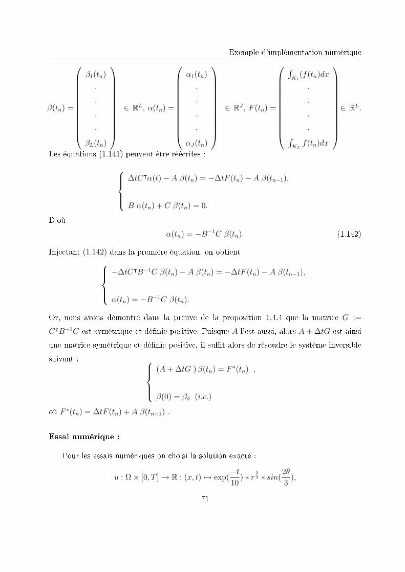
Exemple d'implémentation numérique
β(tn) =
β1(tn)
····
βL(tn)
∈ RL, α(tn) =
α1(tn)
····
αJ(tn)
∈ RJ , F (tn) =
∫K1
(f(tn)dx
····∫
KLf(tn)dx
∈ RL.
Les équations (1.141) peuvent être réécrites :
∆tCᵀα(t)− A β(tn) = −∆tF (tn)− A β(tn−1),
B α(tn) + C β(tn) = 0.
D'où
α(tn) = −B−1C β(tn). (1.142)
Injectant (1.142) dans la première équation, on obtient−∆tCᵀB−1C β(tn)− A β(tn) = −∆tF (tn)− A β(tn−1),
α(tn) = −B−1C β(tn).
Or, nous avons démontré dans la preuve de la proposition 1.4.4 que la matrice G :=
CᵀB−1C est symétrique et dénie positive. Puisque A l'est aussi, alors A+ ∆tG est ainsi
une matrice symétrique et dénie positive, il sut alors de résoudre le système inversible
suivant : (A+ ∆tG ) β(tn) = F ∗(tn) ,
β(0) = β0 (i.c.)
où F ∗(tn) = ∆tF (tn) + A β(tn−1) .
Essai numérique :
Pour les essais numériques on choisi la solution exacte :
u : Ω× [0, T ] → R : (x, t) 7→ exp(−t10
) ∗ r23 ∗ sin(
2θ
3),
71

Équation de la chaleur instationnaire
où (r, θ) désigne les coordonnées polaires standards, avec r =√x2
1 + x22 et θ ∈
]0,
3π
2
[telle
que sin θ =x2
r. l'analyse mathématique précédente a été faite pour l'équation de la chaleur
avec des conditions de Dirichlet homogènes sur le bord ; cependant avec des modications
mineures on obtient une forme équivalente dans le cas des conditions aux bord de type
Dirichlet non homogènes. On a tracé la solution approchée de cette fonction (voir gure
1.5) pour T = 1, les gures 1.3 et 1.4 représentent respectivement ~pnh,x et ~pn
h,y à l'instant
T = 1 :
Ω
Fig. 1.3 ~pnh,x
y
x
Fig. 1.4 ~pnh,y
On prend comme pas de temps xe ∆t = 0.1 :
Maillages utilisés : On a utilisé 2 séries de maillages, une série de maillages uniformes
et une autre de maillages ranés.
La série de maillages uniformes est tout simplement obtenue en subdivisant chaque côté du
domaine Ω en n segments égaux et en coupant chaque carré obtenu en deux pour obtenir
des triangles (voir gure 1.6 où n = 4).
La série de maillages ranés doit remplir les conditions de ranement de maillage en
vue de la restauration de l'ordre de convergence optimal de la méthode. Pour obtenir un
maillage rané, nous utilisons la technique de ranement de maillage de Raugel [11]. Or
on sait que pour tout t ∈ [0, T ] , u (t) ∈ H2,α (Ω) pour α > 1− πω
= 1− π3π2
= 13. On peut
72

Exemple d'implémentation numérique
Fig. 1.5 Solution approchée
-1
-0.5
0
0.5
1
-1 -0.5 0 0.5 1
Fig. 1.6 Maillage Uniforme
-1
-0.5
0
0.5
1
-1 -0.5 0 0.5 1
Fig. 1.7 Maillage Rané
donc choisir α = 0.375 ce qui implique :
β :=1
1− α= 1.6.
(voir gure 1.7 où où n = 4).
73

Équation de la chaleur instationnaire
Résultats
Pour les erreurs ||u (tn)− unh||0,Ω et ||~p (tn)− ~pn
n||0,Ω, nous obtenons :
Maillage rané Maillage uniforme
n
2
4
8
16
32
64
||u (tn)− unh||0,Ω
1.91e-01
4.97e-02
2.47e-02
1.23e-02
6,16e-03
3,08e-03
||~p (tn)− ~pnn||0,Ω
1.55e− 01
9, 10e− 02
5, 12e− 02
2, 81e− 02
1, 52e− 02
8, 15e− 03
||u (tn)− unh||0,Ω
1,04e-01
5,20e-02
2,59e-02
1,29e-02
6,43e-03
3,21e-03
||~p (tn)− ~pnn||0,Ω
1, 73e− 01
1, 16e− 01
7, 54e− 02
4, 84e− 02
3, 08e− 02
1, 95e− 02
On peut démontrer que pour cette famille régulière de traingulaion, il existe deux
constante strictement positives c1, c2 (c1 < c2) indépendantes de n tels que c1n≤ h :=
maxK∈Th
dian(K) ≤ c2n. Et pour montrer que : Erreur = chP , nous utilisons le logarithme,
on a donc ln(Erreur) = −p ln(n) + ln(c′). En traçant donc le logarithme des erreurs en
fonction du logarithme de n, on obtiendra une droite dont le coecient directeur sera le taux
de convergence p. Ces droites sont tracées dans la gure 1.8 pour l'erreur ||u (tn)− unh||0,Ω
et la gure 1.9 pour l'erreur ||~p (tn)− ~pnn||0,Ω
.
Pour la seconde erreur, on voit bien que les maillages uniformes ne présentent qu'un
taux de convergence de p = 23alors que les maillages ranés présentent un ordre optimal
de p = 1.
Par contre, pour la première erreur, on a un taux de convergence de p = 1 pour les
deux séries de maillages.
Précisions : Nous précisons que l'erreur calculée dépend de h mais aussi de ∆t et même
si nous sommes en schéma implicite où nous n'avons pas ce CFL. Nous avons donc pris un
pas de temps susamment petit pour ne pas voir la dépendance des erreurs en fonction
du temps. Nous avons aussi dû prendre une fonction pour laquelle l'erreur en temps sera
négligeable par rapport à l'erreur en espace, au moins jusqu'au n le plus grand que nous
ayons pris.
74

Exemple d'implémentation numérique
0.5 1 1.5 2 2.5 3 3.5 4 4.5−6
−5.5
−5
−4.5
−4
−3.5
−3
−2.5
−2
−1.5
log(n)
|| u
− u h ||
0, Ω
, t=T
raffinéuniforme
1
1
Fig. 1.8 ||u (tn)− unh||0,Ω
75

Équation de la chaleur instationnaire
0.5 1 1.5 2 2.5 3 3.5 4 4.5−5
−4.5
−4
−3.5
−3
−2.5
−2
−1.5
log(n)
|| p
− p h ||
0, Ω
, t=T
raffinéuniforme
1
1
1
2 / 3
Fig. 1.9 ||~p (tn)− ~pnn||0,Ω
76

Chapitre 2
Équations de Stokes instationnaires
2.1 Introduction
Dans ce chapitre, on se propose d'établir des estimations d'erreurs a priori pour le
système de Stokes instationnaire pour un uide visqueux incompressible dans un domaine
polygonal en utilisant la méthode d'éléments nis mixte duale en espace et le schéma d'Eu-
ler implicite en temps : pour cela nous introduisant en outre des inconnues traditionnelles :
la vitesse −→u (t) et la pression p (t), la nouvelle variable σ (t) := ∇~u (t) représentant le
tenseur gradient du champ des vitesses à l'instant t. Nous approximons chacune des deux
lignes de σ (t) par un champ de vecteurs de Raviart-Thomas de degré 0 sur chaque triangle
K de la triangulation, avec continuité de la composante normale aux interfaces. La pression
p (t) est approximée par une constante sur chaque triangle de la triangulation et la vitesse−→u (t) par un champ de vecteurs constant sur chaque triangle. Notons que Claes Johnson
et Vidar Thomée [10] traitent aussi le problème de stokes instationnaire mais en utilisant
la méthode symétrique, d'autant plus que leurs majoration d'erreur théorème 4.1 p. 71-72
ne fait pas apparaître clairement l'estimation d'erreur sur la pression et elles supposent
indirectement que ∇~ut(s) est dans H1 pour s dans [0, T ]. Précisons aussi que les espaces
d'approximations ne sont pas les mêmes puisqu'ils considèrent des éléments de base P 1,
alors que le choix du plus pas degré serait plus adapter. Et en raison du coin réentrant
du domaine polygonal D, nous imposons à la famille de triangulations un ranement de
77

Équations de Stokes instationnaires
maillage approprié an de restaurer l'ordre de convergence optimal 1 de la méthode en
espace. En seconde partie on étudie la stabilité du problème complètement discrétisé à
l'aide du schéma de Euler implicite, nous démontrons enn des estimées d'erreur d'ordre
1 en temps et en espace.
2.2 Domaine ouvert borné lipschitzien
2.2.1 Position du problème
Soit Ω un domaine borné lipschitzien dans R2, posons Q := Ω×]0, T [, avec T > 0.
On considère le problème de Stokes instationnaire pour un uide visqueux incompressible
conné dans Q : étant donné ~f = (f1, f2) ∈ L2(0, T ; (L2(Ω))2) une densité massique de
forces extérieures, trouver des fonctions ~u = (u1, u2) ∈ H1(0, T ; (H10 (Ω))2), le champ de
vitesse du uide, et p ∈ L2(0, T ;L20(Ω)), sa pression, solution du problème de Stokes :
~ut(x, t)− ν∆~u(x, t) +→
grad p(x, t) = ~f(x, t) dans Q,
div ~u(x, t) = 0 dans Q,
~u(x, t) = 0 sur Σ := ∂Ω×]0, T [,
~u(x, 0) = ~u0(x) pour x ∈ Ω,
(2.1)
En introduisant la variable σ = grad ~u, on peut réécrire les équations de Stokes sous la
forme :
~ut − div(νσ − pδ) = ~f dans Q,
div ~u = 0 dans Q,
~u = 0 sur Σ,
~u(0) = ~u0 dans Ω,
(2.2)
78

Domaine ouvert borné lipschitzien
où δ désigne le tenseur identité donné par δ =
1 0
0 1
. Rappelons que τ étant un
tenseur, div τ désigne le champ de vecteurs de composante (div τ)i =∑2
j=1∂τij
∂xj(i = 1, 2).
2.2.2 Existence, unicité et régularité de la solution
Avant de donner la preuve de l'existence de l'unicité ainsi que de la régularité de la
solution faible de (2.1), soit
V :=v ∈ (H1(Ω))2; div ~v = 0
.
Nous avons le résultat d'existence suivant :
Théorème 2.2.1 ([46] théorème III.1.1 p.254)
Etant donné ~f ∈ L2(0, T ;L2(Ω)2) et ~u0 ∈ L2(Ω)2 à divergence nulle. Il existe une unique
fonction ~u ∈ L2(0, T ;V ) ∩ C([0, T ];L2(Ω)2) telle que ~u(0) = ~u0 , ~u′ ∈ L2(0, T ;V ′) telle
qued
dt(~u,~v) + ν
∫Ω
∇~u : ∇~v =
∫Ω
~f · ~v, ∀~v ∈ V. (2.3)
Soit alors (~u, p) la solution faible du problème de Stokes instationnaire (2.1), nous
avons :
Théorème 2.2.2 Sous les hypothèses : Ω étant l'ouvert borné lipschitzien, ~f ∈ L2(0, T ;L2(Ω)2)
et ~u0 ∈ V , on a :
~u ∈ H1(0, T ;L2(Ω)2). (2.4)
De plus il existe une et une seule fonction p ∈ L2(0, T ;L20(Ω)) que l'on appelle pression
telle que :
d
dt(~u,~v) + ν
∫Ω
∇~u : ∇~v −∫
Ω
p div~v =
∫Ω
~f · ~v, ∀~v ∈ H10 (Ω)2. (2.5)
Preuve: V étant séparable, il existe donc une suite ~w1, ~w2, . . . , ~wm, . . . de vecteurs linéai-
rement indépendants qui est totale dans V . Soit ~um(t) =∑m
i=1 gim(t) ~wi, la solution du
problème de Cauchy pour le système d'équations diérentielles
79
Équations de Stokes instationnaires
∫Ω
d~um
dt(t) · ~wj dx+ ν
∫Ω
∇~um(t) : ∇~wj dx =
∫Ω
~f(t) · ~wj dx, ∀j = 1, ...,m (2.6)
de condition initiale ~um(0) = ~u0m, que l'on précisera dans la suite.~u′m(t), étant une combinaison linéaire de ~w1, ..., ~wm il suit de (2.6)
∥∥∥~u′m(t)∥∥∥2
0,Ω+ ν
∫Ω
∇~um(t) : ∇~u′m(t) dx =
∫Ω
~f(t) · ~u′m(t) dx.
Maisd
dt‖~um(t)‖2
H10 (Ω)2 = 2
∫Ω
∇~um(t) : ∇~u′m(t) dx.
D'où
2∥∥∥~u′m(t)
∥∥∥2
0,Ω+ ν
d
dt‖~um(t)‖2
H10 (Ω)2 ≤
∥∥∥~f(t)∥∥∥2
0,Ω+∥∥∥~u′m(t)
∥∥∥2
0,Ω,
ce qui entraîne ∥∥∥~u′m(t)∥∥∥2
0,Ω+ ν
d
dt‖~um(t)‖2
H10 (Ω)2 ≤
∥∥∥~f(t)∥∥∥2
0,Ω.
Intégrons de 0 à T l'inégalité précédente :∫ T
0
∥∥∥~u′m(t)∥∥∥2
0,Ωdt+ ν ‖~um(T )‖2
H10 (Ω)2 ≤ ν ‖~um(0)‖2
H10 (Ω)2 +
∫ T
0
∥∥∥~f(t)∥∥∥2
0,Ωdt.
Si ~um(0) converge vers ~u(0) dans la norme de H10 (Ω)2, alors on aura ‖~um(0)‖H1
0 (Ω)2 .
‖~u(0)‖H10 (Ω)2 . Et donc∫ T
0
∥∥∥~u′m(t)∥∥∥2
0,Ωdt . ν ‖~u(0)‖2
H10 (Ω)2 +
∫ T
0
∥∥∥~f(t)∥∥∥2
0,Ωdt.
Donc la suite(~u′m(t)
)m≥1
est bornée dans L2(0, T ; (L2(Ω))2) ce qui nous permet d'armer
qu'il existe un certain ~v ∈ L2(0, T ; (L2(Ω))2) et une sous-suite que nous notons encore ~u′m
par un abus de notation usuel telle que ~u′mw ~v dans L2(0, T ; (L2(Ω))
2) (au sens faible).
Soit alors ϕ ∈ D (]0, T [) et J∗ ∈ V ′. L'application de
L2(0, T ;V ) −→ R
~g 7−→ −∫ T
0
〈~g(t), J∗〉V,V ′ ϕ′(t) dt,
80

Domaine ouvert borné lipschitzien
est une forme linéaire continue sur L2(0, T ;V ). En eet :∣∣∣∣−∫ T
0
〈~g(t), J∗〉V,V ′ ϕ′(t) dt
∣∣∣∣ ≤∫ T
0
‖~g(t)‖V ‖J∗‖V ′ |ϕ′(t) | dt
≤ ‖J∗‖V ′
(∫ T
0
‖~g(t)‖2V dt
) 12(∫ T
0
|ϕ′(t) |2 dt) 1
2
= ‖J∗‖V ′ ‖~g‖L2(0,T ;V ) ‖ϕ′‖L2(0,T )
= C ‖~g‖L2(0,T ;V ) .
Comme ~umw ~u dans L2(0, T ;V ) d'après le théorème d'existence 2.2.1, il s'en suit que
−∫ T
0
〈~um(t), J∗〉V,V ′ ϕ′(t) dt −→ −∫ T
0
〈~u(t), J∗〉V,V ′ ϕ′(t) dt. (2.7)
D'autre part, si l'on prend J∗ ∈ (L2(Ω)2)∗, alors l'application de
L2(0, T ;L2(Ω)2) −→ R
~h 7−→ −∫ T
0
⟨~h(t), J∗
⟩L2(Ω)2,(L2(Ω)2)∗
ϕ(t) dt,
est une forme linéaire continue sur L2(0, T ; (L2(Ω))2). Comme ~u′m
w ~v dans L2(0, T ; (L2(Ω))
2),
alors
∫ T
0
⟨~u′m (t) , J∗
⟩L2(Ω)2,(L2(Ω)2)∗
ϕ(t) dt −→∫ T
0
〈~v(t), J∗〉L2(Ω)2,(L2(Ω)2)∗ ϕ(t) dt. (2.8)
Or, si J∗ ∈ (L2(Ω)2)∗, cela implique que J∗|V ∈ V ′, donc on a
∫ T
0
⟨~u′m(t), J∗
⟩ϕ(t) dt =
⟨∫ T
0
~u′m (t)ϕ(t) dt, J∗⟩
= −⟨∫ T
0
~um (t) ϕ′(t) dt, J∗⟩
= −∫ T
0
〈~um(t), J∗〉 ϕ′(t) dt→ −∫ T
0
〈~u(t), J∗〉 ϕ′(t) dt .(2.9)
81

Équations de Stokes instationnaires
par (2.7).
De (2.9) et (2.8) suit :
−∫ T
0
〈~u(t), J∗〉 ϕ′(t) dt =
∫ T
0
〈~v(t), J∗〉 ϕ(t) dt, ∀J∗ ∈(L2(Ω)2
)∗.
D'où
−∫ T
0
~u(t)ϕ′(t) dt =
∫ T
0
~v(t)ϕ(t) dt, ∀ϕ ∈ D(]0, T [).
Ceci démontre (~u)′ = ~v au sens faible. Comme l'on sait que ~v ∈ L2(0, T ; (L2(Ω))2), on a
(~u)′ ∈ L2(0, T ; (L2(Ω))2). Nous avons donc démontré que
d~u
dt∈ L2(0, T ;
(L2(Ω)
)2). (2.10)
Venons-en maintenant à l'existence de la fonction pression p. Posons :
~q = ~f − d~u
dt+ υ∆~u. (2.11)
Comme
~u ∈ H1(0, T ;(H1
0 (Ω))2
),
il s'en suit que :
∆~u ∈ L2(0, T ;(H−1(Ω)
)2).
De l'équation (2.11) et de (2.10) suit que ~q ∈ L2(0, T ; (H−1(Ω))2). Mais l'opérateur
~∇ : L20(Ω) −→
(H−1(Ω)
)2est un isomorphisme de L2
0(Ω) sur V (le polaire de V ) ([15], lemme I.2.1 p.22). Or ~q(t) ∈ V ,∀′t ∈]0, T [ par (2.11) et (2.3). Donc il existe p(t) ∈ L2
0(Ω) tel que ~q(t) = ~∇p(t).Notons
(~∇)−1
: V −→ L20(Ω) l'opérateur inverse de ~∇ : L2
0(Ω) V . Donc
p(t) =(~∇)−1
~q(t) .
Comme ~q ∈ L2(0, T ; (H−1(Ω))2), il s'en suit que p ∈ L2(0, T ;L2
0(Ω)). De (2.11) et ~q = ~∇psuit (2.5).
82
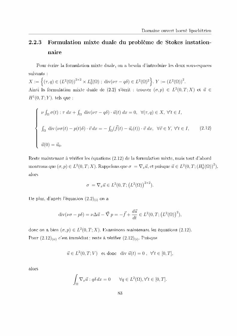
Domaine ouvert borné lipschitzien
2.2.3 Formulation mixte duale du problème de Stokes instation-
naire
Pour écrire la formulation mixte duale, on a besoin d'introduire les deux sous-espaces
suivants :
X :=
(τ, q) ∈ (L2(Ω))2×2 × L2
0(Ω) ; div(ντ − qδ) ∈ L2(Ω)2, Y := (L2(Ω))
2.
Ainsi la formulation mixte duale de (2.2) s'écrit : trouver (σ, p) ∈ L2(0, T ;X) et ~u ∈H1(0, T ;Y ), tels que :
ν∫
Ωσ(t) : τ dx+
∫Ω
div(ντ − qδ) · ~u(t) dx = 0, ∀(τ, q) ∈ X, ∀′t ∈ I,
∫Ω
div (νσ(t)− p(t)δ) · ~v dx = −∫
Ω(~f(t)− ~ut(t)) · ~v dx, ∀~v ∈ Y, ∀′t ∈ I,
~u(0) = ~u0.
(2.12)
Reste maintenant à vérier les équations (2.12) de la formulation mixte, mais tout d'abord
montrons que (σ, p) ∈ L2(0, T ;X). Rappelons que σ = ∇x~u, et puisque ~u ∈ L2(0, T ; (H10 (Ω))
2),
alors
σ = ∇x~u ∈ L2(0, T ;(L2(Ω)
)2×2).
De plus, d'après l'équation (2.2)(i) on a
div(νσ − pδ) = ν∆~u− ~∇ p = −~f +d~u
dt∈ L2(0, T ;
(L2(Ω)
)2),
donc on a bien (σ, p) ∈ L2(0, T ;X). Examinons maintenant les équations (2.12).
Pour (2.12)(ii) c'est immédiat ; reste à vérier (2.12)(i). Puisque
~u ∈ L2(0, T ;V ) et donc div ~u(t) = 0 , ∀′t ∈ [0, T ],
alors ∫Ω
∇x~u : qδ dx = 0 ∀q ∈ L2(Ω),∀′t ∈ [0, T ].
83

Équations de Stokes instationnaires
D'où
ν
∫Ω
σ(t) : τ dx =
∫Ω
∇x~u(t) : (ντ − qδ)dx ∀(τ, q) ∈ X,∀′t ∈ [0, T ]
=
〈(ντ − qδ) · ~n, ~u(t)〉
H− 12 (Γ)2,H
12 (Γ)2
−∫
Ω
~u(t) : div(ντ − qδ)dx
,
= −∫
Ω
~u(t) · div(ντ − qδ)dx
puisque ~u(t) ∈ (H10 (Ω))
2,∀′t ∈ [0, T ].
Donc
ν
∫Ω
σ(t) : τ dx+
∫Ω
~u(t) · div(ντ − qδ) · ~u(t)dx = 0, ∀(τ, q) ∈ X, ∀′t ∈ [0, T ].
Donc on a démontré que si (~u, p) est une solution de (2.2) alors ((σ, p), ~u) est une solution de
la formulation mixte (2.12) pourvu que ~u0 ∈ V et que Ω soit un ouvert borné lipschitzien.
Reste à montrer l'unicité de cette solution et par conséquent l'équivalence entre le problème
(2.2) et la formulation mixte (2.12).
Soient alors ((σ1, p1), ~u1) , ((σ2, p2), ~u2) deux solutions de la formulation mixte (2.12).
Considérons la diérence ((σ, p), ~u) := ((σ1 − σ2, p1 − p2), ~u1 − ~u2) de ces deux solutions.
Elle vérie les équations suivantes :
ν∫
Ωσ(t) : τ dx+
∫Ω
div(ντ − qδ) · ~u(t)dx = 0 ∀(τ, q) ∈ X, ∀′t ∈ I ,
∫Ω
div (νσ(t)− p(t)δ) · ~v dx =∫
Ω~ut(t) · ~v dx ∀~v ∈ Y, ∀′t ∈ I,
~u(0) = 0.
(2.13)
Prenons (τ, q) = (σ(t), p(t)) dans l'équation (2.13)(i). Puisque (σ(t), p(t)) ∈ X ∀′t ∈ [0, T ],
alors
ν
∫Ω
|σ(t)|2 dx+
∫Ω
div (νσ(t)− p(t)δ) · ~u(t)dx = 0, ∀′t ∈ I. (2.14)
Prenons maintenant ~v = ~u(t) dans (2.13)(ii), ce qui est permis puisque ∀′t ∈ [0, T ] : ~u(t) ∈
84

Domaine polygonal
Y = L2(Ω)2 ; ceci nous donne : ∀′t ∈ [0, T ]∫Ω
div (νσ(t)− p(t)δ) · ~u(t) dx =
∫Ω
~ut(t) · ~u(t)dx,
=1
2
∫Ω
d
dt|~u(t)|2 dx. (2.15)
De (2.15) et (2.14) suit :
ν
∫Ω
|σ(t)|2 dx+1
2
d
dt
∫Ω
|~u(t)|2 dx = 0 (2.16)
et implique ddt
∫Ω|~u(t)|2 dx ≤ 0, donc
∫Ω|~u(·)|2 dx est décroissante, et comme
∫Ω
|~u(·)|2 dx ∈ H1 ([0, T ]) → C ([0, T ]) ,
avec ~u(0) = 0, cela entraîne que ~u(t) = 0 ∀t ∈ [0, T ]. Par (2.16) on a également σ = 0.
D'autre part, par l'équation (2.13)(ii), on a∫Ω
~∇x p(t) · ~v dx = 0 pour tout ~v ∈(L2(Ω)
)2.
Et puisque (0, p(t)) ∈ X, donc p(t) ∈ H1(Ω) ∩ L20(Ω). Choisissant ~v = ~∇x p(t), il s'en
suit ~∇x p(t) = 0 et donc p(t) = constante ∀′t ∈ [0, T ], mais comme p(t) ∈ L20(Ω), la seule
possibilité est p = 0.
2.3 Dans un domaine polygonal
Dans la suite, on suppose que Ω est un domaine de R2 à bord polygonal : ∂Ω := ∪Nj=1Γj,
où Γj est un segment de droite ouvert ∀ j = 1, 2, ..., N . On suppose aussi que Ω n'a qu'un
seul angle non convexe dont la mesure est notée ω ; par translation éventuelle on peut
supposer que le sommet de cet angle est situé à l'origine.
85

Équations de Stokes instationnaires
2.3.1 Régularité en espace de la solution
Supposant que ~f ∈ L2(0, T ;L2(Ω)2) et ~u0 ∈ H1 (Ω)2 avec div ~u0 = 0, il suit de la
proposition 1.2 p.267 du livre de Temam [46] que ~u′ ∈ L2(0, T ;L2(Ω)2). D'où
−ν∆~u+ ~∇p = ~f − d~u
dt∈ L2(0, T ;L2(Ω)2),
div ~u(t) = 0 dans Ω,
~u(t) = 0 sur ∂Ω.
(2.17)
De la régularité de la solution du problème stationnaire, suit alors que ~u ∈ L2(0, T ;H2,α(Ω)2)
et p ∈ L2(0, T ;H1,α(Ω) ∩ L20(Ω)) pour α ∈ ]1− η0(ω), 1[ où
η0(ω) = infξ ∈ R+
∗ ; z = ξ + iη vérie sin2 ωz = z2 sin2 ω, z 6= 1.
Supposons maintenant que ~f ∈ H1(0, T ;L2(Ω)2), que ~f (0) + ν∆~u0 ∈ H1 (Ω)2 et que
div ~f (0) = 0.
Soit (~w, ζ) ∈ L2 (0, T ;V )× L2 (0, T ;L20 (Ω)) la solution au sens faible ([46] p.253) de
d~w
dt(t)− ν∆~w (t) + ~∇ζ (t) = ~f ′ (t) , ∀′t ∈ ]0, T [
div ~w(t) = 0 , ∀′t ∈ ]0, T [
~w(0) = ~f (0) + ν∆~u0 .
Rappelons ([46] p.251) que V =~v ∈ H1 (Ω)2 ; div~v = 0
. Par le raisonnement ci-dessus
~w′ ∈ L2(0, T ;L2(Ω)2) et (~w, ζ) ∈ L2 (0, T ;H2,α(Ω)2)× L2 (0, T ;H1,α(Ω) ∩ L20(Ω)) .
Posons ~v (t) = ~u0 +∫ t
0~w (s) ds et q (t) =
∫ t
0ζ (s) ds.
86

Problème semi-discret
On vérie qu'au sens faible :
d~v
dt(t)− ν∆~v (t) + ~∇q (t) = ~f (t) , ∀′t ∈ ]0, T [
div~v(t) = 0 dans Ω, ∀′t ∈ ]0, T [
~v(0) = ~u0 .
Par unicité ~u = ~v et doncd~u
dt= ~w ∈ L2
(0, T ;H2,α (Ω)2) . De même p = q et donc
dp
dt= ζ ∈ L2 (0, T ;H1,α(Ω) ∩ L2
0(Ω)) .
Nous avons donc démontré le résultat de régularité suivant :
Proposition 2.3.1 Supposons ~f ∈ H1(0, T ;L2(Ω)2), que div ~f (0) = 0, et que la condition
initiale ~u0 ∈ V du problème de Stokes instationnaire satisfasse la condition ~f (0)+ ν∆~u0 ∈H1 (Ω)2 .
Alors la solution (~u, p) ∈ L2 (0, T ;V ) × L2 (0, T ;L20 (Ω)) du problème de Stokes instation-
naire appartient à l'espace de Sobolev
H1(0, T ;(H2,α(Ω)
)2)×H1(0, T ;H1,α(Ω)) (2.18)
pour tout α ∈ ]1− η0(ω), 1[ où η0(ω) = infξ ∈ R+∗ ; z = ξ + iη vérie sin2 ωz = z2 sin2 ω,
z 6= 1.
2.4 Problème semi-discret
Pour introduire la formulation mixte semi-discrète du problème (2.12), considérons une
famille régulière de triangulations (Th)h de Ω, et dénissons des sous-espaces approximants
Xh et Yh des espaces X et Y :
Xh : =(τh, qh) ∈ X ; τh(i,·) ∈ RT0(K) ∀i = 1, 2 et qh|K ∈ P0(K), ∀K ∈ Th
,
Yh : =~vh ∈ Y ; ~vh|K ∈ (P0(K))2 , ∀K ∈ Th
.
87

Équations de Stokes instationnaires
P0 dénote l'espace des fonctions constantes sur K et RT0(K) dénote l'espace vectoriel des
champs de Raviart-Thomas du plus bas degré sur K déni par :
RT0(K) = v : K → R;∃ a, b, c ∈ R : v(x) = (a, b) + c(x1, x2),∀x = (x1, x2) ∈ K
Finalement, on a ~u0,h = Ph~u0 où Ph est l'opérateur de projection de (L2(Ω))2 sur
∏K∈Th
(P0(K))2.
On peut maintenant introduire le problème approché : trouver (σh, ph) ∈ L2(0, T ;Xh),
~uh ∈ L2(0, T ;Yh) tels que :
ν∫
Ωσh(t) : τh dx+
∫Ω
div(ντh − qhδ) · ~uh(t) dx = 0, ∀ (τh, qh) ∈ Xh, ∀′t ∈ I,
∫Ω
div (νσh(t)− ph(t)δ) · ~vh dx = −∫
Ω(~f(t)− ~uh,t(t)) · ~vh dx, ∀~vh ∈ Yh, ∀′t ∈ I,
~uh(0) = ~u0,h.
(2.19)
Avant d'examiner le problème semi-discret (2.19) nous allons tout d'abord rappeler
certains résultats relatifs aux équations de Stokes stationnaires (Cf. [9]) .
Nous considérons les équations de Stokes stationnaires :−ν∆~u+
−→gradp = ~f dans Ω,
div ~u = 0 dans Ω,
~u = ~0 sur Γ.
(2.20)
La formulation mixte de ce dernier problème consiste à trouver (σ, p) ∈ X et ~u ∈ Y tels
que ν∫
Ωσ : τ dx+
∫Ωdiv(ντ − qδ) · ~udx = 0 , ∀ (τ, q) ∈ X,
∫Ωdiv (νσ − pδ) · ~v dx = −
∫Ω~f · ~v dx ∀~v ∈ Y.
(2.21)
Il est clair que la solution (~u, p) de (2.20) vérie (σ, p) ∈ X, où σ = ∇~u et donc que
((σ, p) , ~u) est une solution de (2.21). De plus, d'après [9], la formulation mixte (2.21)
admet une solution unique.
Le problème approché pendant de (2.21) consiste à trouver ((σh, ph) , ~uh) ∈ Xh × Yh tels
88

Problème semi-discret
que ν∫
Ωσh : τh dx+
∫Ωdiv(ντh − qhδ) · ~uh dx = 0 , ∀ (τh, qh) ∈ Xh,
∫Ωdiv (νσh − ph δ) · ~vh dx = −
∫Ω~f · ~vh dx , ∀~vh ∈ Yh.
(2.22)
L'existence et l'unicité de la solution de ce dernier problème sont des conséquences de la
proposition 4.1.2 de [9].
Étant donné ~f ∈ (L2(Ω))2, on peut dénir l'opérateur T par
T : Y −→ X × Y : ~f 7→ T ~f =(T1
~f, T2~f)
= ((σ, p) , ~u) (2.23)
où ((σ, p) , ~u) est la solution de (2.21) .
Aussi, nous dénissons l'opérateur Th par
Th : Y −→ Xh × Yh : ~f 7→ Th~f =
(Th,1
~f, Th,2~f)
= ((σh, ph) , ~uh) (2.24)
où ((σh, ph) , ~uh) est la solution de (2.22). Finalement, on démontre dans [9], le résultat
suivant sur les estimations d'erreurs à priori :
Théorème 2.4.1 [12] Soit Th une famille régulière de triangulations sur Ω, jouissant
des propriétés (i) et (ii) de la proposition 1.4.6, pour un α ∈ ]1− η0(ω), 1[. Soient T ~f =
((σ, p) , ~u) et Th~f = ((σh, ph) , ~uh). Alors (σ, p) ∈ (H1,α(Ω))
4 × (H1,α(Ω) ∩ L20(Ω)) , et il
existe une constante C > 0 indépendante de h telle que
‖σ − σh‖0,Ω ≤ Ch(|~u|H2,α(Ω)2 + |p|H1,α(Ω)
), (2.25)
‖p− ph‖0,Ω ≤ Ch(|~u|H1,α(Ω)2 + |p|H1,α(Ω)
), (2.26)
‖~u− ~uh‖0,Ω ≤ Ch(|~u|H2,α(Ω)2 + |p|H1,α(Ω) + |~u|H1(Ω)2
). (2.27)
Maintenant, on est en mesure de démontrer l'existence et l'unicité de la solution du
problème instationnaire semi-discret (2.19) ainsi que des estimations d'erreurs à priori.
Proposition 2.4.2 Le problème (2.19) admet une et une seule solution ((σh, ph) , ~uh)
dans L2(0, T ;Xh)× L2(0, T ;Yh).
89

Équations de Stokes instationnaires
Preuve: Soit ~g ∈ Y. Considérons les opérateurs Th,1 et Th,2 dénis dans (2.22) :
Th,1 : Y −→ Xh et Th,2 : Y −→ Yh
~g 7−→ Th,1~g = (σh, ph) ~g 7−→ Th,2~g = ~uh
où ((σh, ph) , ~uh) désigne donc la solution du problème mixte stationnaire semi-discret sui-
vant : ν∫
Ωσh : τh dx+
∫Ω
(ντh − qhδ) · ~uh dx = 0, ∀ (τh, qh) ∈ Xh,
∫Ω
(νσh − phδ) · ~vh dx = −∫
Ω~g · ~vh dx , ∀~vh ∈ Yh.
(2.28)
Ce problème possède une et une seule solution ∀~g ∈ (L2(Ω))2
:= Y. Revenons au problème
d'évolution discret (2.19), si on applique la dénition de Th, on obtient :(σh(t), ph(t)) = Th,1
(~f(t)− d~uh
dt(t))
~uh(t) = Th,2
(~f(t)− d~uh
dt(t)).
D'où
~uh(t) + Th,2d~uh
dt(t) = Th,2
~f(t) et ~uh(0) = ~u0,h,
Montrer que ce problème possède une et une seule solution revient, en fait, comme nous le
verrons plus loin, à montrer que Th,2 est un opérateur déni positif sur Yh. Prenons donc
un élément ~fh ∈ Yh, et considérons le problème mixte discret stationnaire de donnée ~fh :ν∫
Ωσh : τh dx+
∫Ω
(ντh − qhδ) · ~uh dx = 0 , ∀ (τh, qh) ∈ Xh,
∫Ω
(νσh − phδ) · ~vh dx = −∫
Ω~fh · ~vh dx , ∀~vh ∈ Yh.
(2.29)
Alors Th,2~fh = ~uh et Th,1
~fh = (σh, ph), et on a∫Ω
(Th,2
~fh
)· ~fh dx =
∫Ω
~fh · ~uh dx = −∫
Ω
(νσh − phδ) · ~uh dx
= ν
∫Ω
σh : σh dx = ν
∫Ω
|σh|2 ≥ 0.
En particulier∫
Ω(Th,2
~fh) · ~fh dx = 0 implique σh = 0.
Mais si σh = 0, et comme (νσh − phδ) ∈ H(,Ω), alors ph ∈ H1(Ω) implique ~∇ph ∈ (L2(Ω))2.
90

Problème semi-discret
Mais comme ph|K ∈ P0(K), il s'en suit ~∇ph = 0 dans Ω et donc ph = constante dans Ω.
Mais puisque ph ∈ L20(Ω), alors ph = 0. Donc si σh = 0, cela entraîne que ~fh = 0 par
l'équation (2.29)(ii). En conclusion, si ~fh 6= 0 alors
ν
∫Ω
|σh|2 > 0
et∫
Ω
(Th,2
~fh
)· ~fh dx > 0. À fortiori, l'application Th,2|Yh
: Yh −→ Yh est injective donc
inversible.
On conclut que :
~uh(t) = exp(tAh)~u0,h −∫ t
0
exp((t− s)Ah)AhTh,2~f(s)ds
~uh(t) = ~u0,h, avec Ah = −(Th,2|Yh
)−1.
~uh étant ainsi déterminé, le système (2.19) peut être employé pour déterminer (σh, ph).
Nous avons donc démontré l'existence et l'unicité de la solution du problème mixte
discret.
2.4.1 Estimations d'erreurs
Notre objectif, dans cette section, est de démontrer certaines estimations d'erreurs.
Dans ce qui suit, ((σ, p), ~u) désigne la solution du problème continu (2.12) et ((σh, ph), ~uh)
désigne la solution du problème semi-discret (2.19). (νσ(t)− p(t)δ) ∈ (L2(Ω))2, ∀′t ∈ I,
car (σ, p) ∈ L2(0, T ;X).
Dans la suite, on a besoin d'introduire l'opérateur d'interpolation de Raviart-Thomas et
l'appliquer à (νσ(t)− p(t)δ). Pour cela il faut que (νσ(t)− p(t)δ) ∈ W 1,q(Ω)4 pour un
certain q > 1, ∀′t ∈ I. Ceci est vrai d'après les hypothèses (2.18).Dénissons :
πh(σ(t), p(t)) :=
(1
ν
[π1
h (νσ(t)− p(t)δ) + ρh (p(t)) δ], ρh (p(t))
), ∀′t ∈ I,
où nous avons ([13] p.87) :
1) ∀K ∈ Th : 1ν
[π1h (νσ(t)− p(t)δ) + ρh (p(t)) δ]|K = 1
ν
[π1
K (νσ(t)− p(t)δ)|K + ρh p(t)|K δ]∈
RT0(K)2 ;
91

Équations de Stokes instationnaires
π1h dénote l'opérateur d'interpolation de Raviart-Thomas [9] et π1
K sa restriction au triangle
K.
2) ρh désigne l'opérateur de projection orthogonale de L20(Ω) sur le sous-espace qh ∈
L20(Ω) qh|K ∈ P0(K), ∀K ∈ Th i.e. :
(ρh q)|K := ρK q :=1
|K|
∫K
q dx, ∀K ∈ Th .
Pour notre étude sur l'estimation d'erreur on va travailler dans le cas où ~uh(0) = Ph~u(0).
On a alors le résultat suivant :
Proposition 2.4.3 Soit (Th)h une famille régulière de triangulations sur Ω, jouissant des
propriétés (i) et (ii) de la proposition 1.4.6. Alors :
‖σ(0)− σh(0)‖0,Ω ≤ ‖σ(0)− σ∗h(0)‖0,Ω . (2.30)
où ((σ(0), p(0)) , ~u(0)) désigne la solution du problème mixte (2.12) à l'instant t = 0, et
(σ∗h(t), p∗h(t)) := πh(σ(t), p(t)).
Preuve: Appliquons l'équation (2.19)(i) à l'instant t = 0. On obtient
ν
∫Ω
σh(0) : τh dx = −∫
Ω
(ντh − qhδ) · ~uh(0) dx ∀ (τh, qh) ∈ Xh,
= −∫
Ω
(ντh − qhδ) · Ph~u(0) dx,
= −∑K⊂Ω
(ντh − qhδ)
∫K
Ph~u(0) dx,
= −∑K⊂Ω
(ντh − qhδ)
∫K
~u(0) dx = −∫
Ω
(ντh − qhδ) · ~u(0) dx.
Par l'équation (2.12)(i) à l'instant t = 0 on a :
−∫
Ω
(ντh − qhδ) · ~u(0) dx = ν
∫Ω
σ(0) : τh dx, ∀ (τh, qh) ∈ Xh ⊂ X,
on a donc ∀ (τh, qh) ∈ Xh,
ν
∫Ω
(σ(0)− σh(0)) : τh dx = 0. (2.31)
92

Problème semi-discret
D'autre part on a
‖σ(0)− σh(0)‖2
0,Ω=
∫Ω
(σ(0)− σh(0)) : (σ(0)− σh(0)) dx,
=
∫Ω
(σ(0)− σ∗h(t)) : (σ(0)− σh(0)) dx+
∫Ω
(σ∗h(t)− σh(0)) : (σ(0)− σh(0)) dx
Si on applique (2.31) avec τh = σ∗h(0)−σh(0) ∈ RT0(K)2 au membre de droite, on obtient :
‖σ(0)− σh(0)‖20,Ω =
∫Ω
(σ(0)− σ∗h(0)) : (σ(0)− σh(0)) dx
≤ ‖σ(0)− σh(0)‖0,Ω ‖σ(0)− σ∗h(0)‖0,Ω .
Par conséquent
‖σ(0)− σh(0)‖0,Ω ≤ ‖σ(0)− σ∗h(0)‖0,Ω .
Remarque 2.4.4 σ(0) a bien un sens car des hypothèses (2.18) suit
~u ∈ C ([0, T ];(H2,α(Ω)
)2)
et donc
σ ∈ C ([0, T ];(H1,α(Ω)
)2×2).
Soit (~u(t), p(t)) la solution de (2.1) , pour t xé. Posons((σh (t) , ph (t)) ; ~uh (t)
)= Th(−ν∆~u (t) + ~gradp (t)),
c'est-à-dire que((σh (t) , ph (t)) ; ~uh (t)
)est la solution du problème semi-discret suivant :
ν∫
Ωσh(t) : τh dx+
∫Ωdiv(ντh − qhδ) · ~uh(t) dx = 0, ,∀ (τh, qh) ∈ Xh,
∫Ωdiv (νσh(t)− ph(t)δ) · ~vh dx+
∫Ω(−ν∆~u(t) + ~gradp(t)) · ~vh dx = 0, ∀′t ∈ I,∀~vh ∈ Yh.
Retournons pour quelques instants au problème continu (2.1) et posons :((σ, p) ; ~u
)= T (−ν∆~u+ ~gradp),
93

Équations de Stokes instationnaires
c'est-à-dire((σ, p) ; ~u
)est la solution du problème suivant :
ν∫
Ωσ(t) : τ dx+
∫Ωdiv(ντ − qδ) · ~u(t) dx = 0 ∀′t ∈ I, ∀ (τ, q) ∈ X,
∫Ωdiv (νσ(t)− p(t)δ) · ~v dx+
∫Ω(−ν∆~u(t) + ~gradp(t)) · ~v dx = 0 ∀′t ∈ I,∀~v ∈ Y.
Comme∂~u
∂t− ν∆~u+ ~grad p = f
on a alors
−ν∆~u+ ~grad p = f − ∂~u
∂t
il s'en suit queν∫
Ωσ(t) : τ dx+
∫Ωdiv(ντ − qδ) · ~u(t) dx = 0 , ∀′t ∈ I, ∀ (τ, q) ∈ X,
∫Ωdiv (νσ(t)− p(t)δ) · ~v dx+
∫Ω(f(t)− ∂~u
∂t(t)) · ~v dx = 0 ,∀′t ∈ I,∀~v ∈ Y,
(2.32)
Et par conséquent, grâce à l'unicité de la solution, on a((σ, p) ; ~u
)= ((σ, p) ; ~u) = T (−ν∆~u+ ~gradp). (2.33)
Dénition 2.4.5 On appelle projection elliptique de ((σ(t), p(t)); ~u(t)) ∀t′ ∈ I, la solution
((σh(t), p(t)); ~uh(t)) du problème mixte semi-discret stationnaire (t xé) suivant :
ν∫
Ωσh(t) : τh dx+
∫Ω
div(ντh − qhδ) · ~uh(t) dx = 0 ∀ (τh, qh) ∈ Xh,
∫Ω
div (νσh(t)− ph(t)δ) · ~vh dx = −∫
Ω(~f(t)− ~ut(t)) · ~vh dx ∀~vh ∈ Yh.
(2.34)
Avant de démontrer le résultat d'approximation de ((σ, p); ~u) par ((σh, ph); ~uh), on a
besoin des estimations d'erreurs entre la solution du problème de Stokes et la projection
elliptique. On a le résultat suivant :
Proposition 2.4.6 Soit (Th)h une famille régulière de triangulations sur Ω, jouissant des
propriétés (i) et (ii) de la proposition 1.4.6 pour un α ∈ ]1− η0(ω), 1[ . Il existe une
constante c > 0 indépendante de h telle que pour tout t ∈ I :
‖σ(t)− σh(t)‖0,Ω ≤ c h(|~u(t)|H2,α(Ω)2 + |p(t)|H1,α(Ω)
), (2.35)
94

Problème semi-discret
‖~u(t)− ~uh(t)‖0,Ω ≤ c h(|~u(t)|H1(Ω)2 + |~u(t)|H2,α(Ω)2 + |p(t)|H1,α(Ω)
)(2.36)
et pour la pression on a :
‖p(t)− ph (t)‖0,Ω ≤ c h(|~u(t)|H2,α(Ω)2 + |p(t)|H1,α(Ω)). (2.37)
Preuve: Ceci résulte immédiatement de la dénition 2.4.5, (2.33) et des estimations
(2.25),(2.26) et (2.27) .
Nous sommes maintenant en mesure de donner l'estimation de l'erreur ‖σ(t)− σh(t)‖0,Ω,
en comparant le problème semi-discret (2.19) avec le problème dénissant la projection el-
liptique (2.34).
Théorème 2.4.7 Soit (Th)h une famille régulière de triangulations sur Ω, jouissant des
propriétés (i) et (ii) de la proposition 1.4.6 pour un α ∈ ]1− η0(ω), 1[. Il existe une
constante c > 0 indépendante de h telle que pour tout t ∈ I :
‖σ(t)− σh(t)‖0,Ω (2.38)
≤ c h
supt≤T
(|~u(t)|H2,α(Ω)2 +|p(t)|H1,α(Ω)
)+
∥∥∥∥d~udt∥∥∥∥
L2(0,T ;H2,α(Ω)2)
+
∥∥∥∥dpdt∥∥∥∥
L2(0,T ;H1,α(Ω))
.
Preuve: Avant de commencer la démonstration, rappelons les deux problèmes (2.19) et
(2.34) :
le problème semi-discret :
ν∫
Ωσh(t) : τh dx+
∫Ω
div(ντh − qhδ) · ~uh(t) dx = 0 ∀ (τh, qh) ∈ Xh, ∀′t ∈ I,
∫Ω
div (νσh(t)− ph(t)δ) · ~vh dx = −∫
Ω(~f(t)− ~uh,t(t)) · ~vh dx ∀~vh ∈ Yh, ∀′t ∈ I,
~uh(0) = Ph~u(0),
(2.39)
et la projection elliptique : ∀′t ∈ Iν∫
Ωσh(t) : τh dx+
∫Ω
div(ντh − qhδ) · ~uh(t) dx = 0 ∀ (τh, qh) ∈ Xh,
∫Ω
div (νσh(t)− ph(t)δ) · ~vh dx = −∫
Ω(~f(t)− ~ut(t)) · ~vh dx ∀~vh ∈ Yh.
(2.40)
95

Équations de Stokes instationnaires
Une soustraction de (2.40) de (2.39), nous donne le système aux erreurs suivant :ν∫
Ωεh(t) : τh dx+
∫Ω
div(ντh − qhδ) · ~θh(t) dx = 0, ∀t ∈ I, ∀ (τh, qh) ∈ Xh,
∫Ω
div (νεh(t)− rh(t)δ) · ~vh dx =∫
Ωddt
(~uh (t)− ~u(t)) · ~vh dx ∀t ∈ I,∀~vh ∈ Yh,
(2.41)
avec
εh = σh − σh , ~θh = ~uh − ~uh , ~ρh = ~u− ~uh et rh = ph − ph.
Ensuite dérivons par rapport à la variable temps la première équation du système (2.41) :
ν
∫Ω
∂εh
∂t(t) : τh dx+
∫Ω
div(ντh − qhδ) ·∂ ~θh
∂t(t) dx = 0, ∀ (τh, qh) ∈ Xh, ∀′t ∈ I (2.42)
En prenant ~vh = 2 ∂ ~θh
∂tdans (2.41)(ii) et (τh, qh) = 2 (εh, rh) dans (2.42), on obtient
2ν∫
Ω∂εh
∂t(t) : εh dx+ 2
∫Ω
div(νεh − rhδ) · ∂ ~θh
∂t(t) dx = 0
−2∫
Ωdiv (νεh(t)− rh(t)δ) · ∂ ~θh
∂t(t)dx+ 2
∫Ω
(∂ ~θh
∂t(t))2
dx = 2∫
Ω∂~ρh
∂t(t) · ∂ ~θh
∂t(t) dx.
(2.43)
Après addition membre à membre des équations du système (2.43), on aboutit à
2ν
∫Ω
∂εh
∂t(t) : εh dx+ 2
∫Ω
(∂ ~θh
∂t(t)
)2
dx = 2
∫Ω
∂~ρh
∂t(t) · ∂
~θh
∂t(t) dx,
Donc
νd
dt
∫Ω
|εh(t)|2 dx+ 2
∫Ω
(∂ ~θh
∂t(t)
)2
dx = 2
∫Ω
∂~ρh
∂t(t) · ∂
~θh
∂t(t) dx
≤ 2
∥∥∥∥∂~ρh
∂t
∥∥∥∥0,Ω
·
∥∥∥∥∥∂ ~θh
∂t
∥∥∥∥∥0,Ω
≤∥∥∥∥∂~ρh
∂t
∥∥∥∥2
0,Ω
+
∥∥∥∥∥∂ ~θh
∂t
∥∥∥∥∥2
0,Ω
.
Et alors
νd
dt
∫Ω
|εh(t)|2 dx+
∥∥∥∥∥d~θh
dt
∥∥∥∥∥2
0,Ω
≤∥∥∥∥d~ρh
dt
∥∥∥∥2
0,Ω
. (2.44)
96

Problème semi-discret
En conclusion on a :d
dt
∫Ω
|εh(t)|2 dx ≤1
ν
∥∥∥∥d~ρh
dt
∥∥∥∥2
0,Ω
. (2.45)
En intégrant (2.45) par rapport à t, nous obtenons∫Ω
|εh(t)|2 dx−∫
Ω
|εh(0)|2 dx ≤1
ν
∫ t
0
∥∥∥∥d~ρh
dt
∥∥∥∥2
0,Ω
(s) ds,
Donc ∫Ω
|εh(t)|2 dx ≤∫
Ω
|εh(0)|2 dx+1
ν
∫ t
0
∥∥∥∥d~ρh
dt
∥∥∥∥2
0,Ω
(s) ds. (2.46)
Or on a
‖εh(0)‖ = ‖σh(0)− σh(0)‖0,Ω ≤ ‖σh(0)− σ(0)‖0,Ω + ‖σ(0)− σh(0)‖0,Ω . (2.47)
D'après (2.30), et la dénition de πh(σ(t), p(t)), on a
‖σh(0)− σ(0)‖0,Ω ≤ ‖σ(0)− σ∗h(0)‖0,Ω
=
∥∥∥∥σ(0)− 1
ν
[π1
h (νσ(0)− p(0)δ) + ρh (p(0)) δ]∥∥∥∥
0,Ω
=
∥∥∥∥1
ν
[(νσ(0)− p(0)) δ − π1
h (νσ(0)− p(0)δ)]+
1
ν(p(0)− ρh (p(0)) δ
∥∥∥∥0,Ω
≤ 1
ν
∥∥(νσ(0)− p(0)δ)− π1h (νσ(0)− p(0)δ)
∥∥0,Ω
+
√2
ν‖p(0)− ρh (p(0))‖0,Ω .
Des estimations d'erreurs d'interpolation contenues dans la démonstration du Théorème
4.1.7 de [9], il s'en suit que
‖σh(0)− σ(0)‖0,Ω ≤ c h ((|~u(0)|H2,α(Ω)2 + |p(0)|H1,α(Ω)
). (2.48)
De (2.47), (2.48) et (2.35) pour t = 0 on a alors :
‖εh(0)‖0,Ω ≤ c h(|~u(0)|H2,α(Ω)2 + |p(0)|H1,α(Ω)
). (2.49)
Revenons maintenant à (2.46) et rappelons que∥∥∥∥∂~ρh
∂t
∥∥∥∥0,Ω
=
∥∥∥∥∥d~udt − d~uh
dt
∥∥∥∥∥0,Ω
.
97

Équations de Stokes instationnaires
Et remplaçant dans (2.46), on aura
‖εh(t)‖20,Ω ≤ ‖εh(0)‖2
0,Ω +1
ν
∫ t
0
∥∥∥∥∥d~udt − d~uh
dt
∥∥∥∥∥2
0,Ω
ds.
Cette dernière estimation et les estimations (2.49) , (2.36) pour le problème dérivé nous
donnent :
‖εh(t)‖20,Ω
≤ c h2
((|~u(0)|H2,α(Ω) + |p(0)|H1,α(Ω)
)2+
(∫ t
0
(
∣∣∣∣∂~u∂t∣∣∣∣2H2,α(Ω)2
+
∣∣∣∣∂~u∂t∣∣∣∣2H1(Ω)2
+
∣∣∣∣∂p∂t∣∣∣∣2H1,α(Ω)
) ds
)).
Alors on a
‖σh(t)− σh(t)‖0,Ω
≤ c h
((|~u(0)|H2,α(Ω) + |p(0)|H1,α(Ω)
)+
∥∥∥∥d~udt∥∥∥∥
L2(0,T ;H2,α(Ω)2)
+
∥∥∥∥dpdt∥∥∥∥
L2(0,T ;H1,α(Ω))
).
Finalement, l'inégalité triangulaire et l'estimation (2.35) nous donnent
‖σ(t)− σh(t)‖0,Ω ≤ ‖σ(t)− σh(t)‖0,Ω + ‖σh(t)− σh(t)‖0,Ω
≤ c h
supt≤T
(|~u(t)|H2,α(Ω) + |p(t)|H1,α(Ω)
)+
∥∥∥∥d~udt∥∥∥∥
L2(0,T ;H2,α(Ω)2)
+
∥∥∥∥dpdt∥∥∥∥
L2(0,T ;H1,α(Ω))
.
Proposition 2.4.8 Soit Th une famille régulière de triangulations sur Ω. Il existe une
constante c > 0 indépendante de h telle que pour tout t ∈ I :
‖~u(t)− ~uh(t)‖0,Ω ≤ c
(inf
~vh∈Yh
‖~u(t)− ~vh‖0,Ω + ‖σ(t)− σh(t)‖0,Ω
). (2.50)
Preuve: La même démonstration que celle employée pour démontrer la proposition 4.1.9
[9]
Théorème 2.4.9 Soit Th une famille régulière de triangulations sur Ω, jouissant des
propriétés (i) et (ii) de la proposition 1.4.6 pour un certain α ∈ ]1− η0(ω), 1[ . Il existe une
98

Problème semi-discret
constante c > 0 indépendante de h telle que pour tout t ∈ I :
‖~u(t)− ~uh(t)‖0,Ω (2.51)
≤ c h
supt≤T
(|~u(t)|H2,α(Ω) + |p(t)|H1,α(Ω)
)+
∥∥∥∥d~udt∥∥∥∥
L2(0,T ;H2,α(Ω)2)
+
∥∥∥∥dpdt∥∥∥∥
L2(0,T ;H1,α(Ω))
.
Preuve: On vient de voir que
‖~u(t)− ~uh(t)‖0,Ω ≤ c
(inf
~vh∈Yh
‖~u(t)− ~vh‖0,Ω + ‖σ(t)− σh(t)‖0,Ω
).
Prenons ~vh = Ph ~u(t) ∈ Yh, où ∀t ∈ I, Ph ~u(t) est la fonction dont la restriction sur chaque
triangle K de la triangulation Th est égale à la moyenne de ~u(t) sur K. À fortiori :
‖~u(t)− ~uh(t)‖0,Ω ≤ c(‖~u(t)− Ph ~u(t)‖0,Ω + ‖σ(t)− σh(t)‖0,Ω
). (2.52)
Or on sait [9] qu'il existe une constante c > 0 indépendante de h telle que pour tout t ∈ I :
‖~u(t)− Ph ~u(t)‖ ≤ c h(|~u(t)|H1(Ω)2
). (2.53)
Par conséquent il suit de (2.52), en utilisant cette dernière estimation et l'estimation (2.38) ,
que :
‖~u(t)− ~uh(t)‖0,Ω
≤ c h
supt≤T
(‖~u(t)‖H2,α(Ω)2 +|p(t)|H1,α(Ω)
)+
∥∥∥∥d~udt∥∥∥∥
L2(0,T ;H2,α(Ω)2)
+
∥∥∥∥dpdt∥∥∥∥
L2(0,T ;H1,α(Ω))
.
Maintenant, estimons l'erreur sur la pression approchée.
Théorème 2.4.10 Soit Th une famille régulière de triangulations sur Ω, jouissant des
propriétés (i) et (ii) de la proposition 1.4.6 pour un certain α ∈ ]1− η0(ω), 1[ . Il existe
une constante C > 0 indépendante de h telle que pour tout t ∈ I :
‖p(·)− ph(·)‖L2(0,T ;L2(Ω)) ≤ C h(‖~u(·)‖L2(0,T ;H2,α(Ω)2) + ‖p(·)‖L2(0,T ;H1,α(Ω))
)+C h
(‖~u(0)‖H2,α(Ω)2 + ‖p(0)‖H1,α(Ω) +
∥∥∥∥d~udt (·)∥∥∥∥
L2(0,T ;H2,α(Ω)2)
+
∥∥∥∥dpdt (·)∥∥∥∥
L2(0,T ;H1,α(Ω))
)
99

Équations de Stokes instationnaires
Preuve: Avant de commencer la démonstration, rappelons le système aux erreurs (2.41) ,ν∫
Ωεh(t) : τh dx+
∫Ω
div(ντh − qhδ) · ~θh(t) dx = 0, ∀t ∈ I, ∀ (τh, qh) ∈ Xh,
∫Ω
div (νεh(t)− rh(t)δ) · ~vh dx =∫
Ωddt
(~uh (t)− ~u(t)) · ~vh dx ∀t ∈ I,∀~vh ∈ Yh,
(2.54)
avec
εh = σh − σh , ~θh = ~uh − ~uh , ~ρh = ~u− ~uh et rh = ph − ph.
Par la formule de Green, pour tout ~v ∈ H10 (Ω)2, on a ∀t ∈ I :
∫Ω
∇rh(t) · ~v dx =
∫Ω
div rh(t)δ · ~v dx
= −∫
Ω
rh(t)δ : ∇~v dx
=
∫Ω
(νεh(t)− rh(t)δ) : ∇~v dx−∫
Ω
νεh(t) : ∇~v dx. (2.55)
Or, il existe C > 0 telle que :∣∣∣∣∫Ω
νεh(t) : ∇~v dx∣∣∣∣ ≤ C ‖εh(t)‖0,Ω · ‖~v‖H1(Ω)2 . (2.56)
On a aussi ∀~v ∈ H10 (Ω)2 :∫
Ω
(νεh(t)− rh(t)δ) : ∇~v dx = −∫
Ω
div (νεh(t) − rh(t)δ) · ~v dx
= −∫
Ω
div (νεh(t) − rh(t)δ) · Ph~v dx
=
∫Ω
(~ut (t)− ~uh,t(t)) · Ph~v dx (2.57)
par (2.54)(ii).
Par conséquent il existe C > 0 telle que :∣∣∣∣∫Ω
(νεh(t)− rh(t)δ) : ∇~v dx∣∣∣∣ ≤ ‖~ut (t)− ~uh,t(t)‖0,Ω · ‖Ph~v‖0,Ω
≤ C ‖~ut (t)− ~uh,t(t)‖0,Ω · ‖~v‖H10 (Ω)2 . (2.58)
100

Problème semi-discret
De (2.55) et des estimations (2.56) et (2.57) , suit :
‖∇rh(t)‖H−1(Ω)2 ≤ C(‖~ut (t)− ~uh,t(t)‖0,Ω + ‖εh(t)‖0,Ω
). (2.59)
D'autre part [47], [15] p.20, il existe une constante C > 0 telle que pour tout w ∈ L20(Ω) :
‖w‖L20(Ω) ≤ C ‖∇w‖H−1(Ω)2 = sup
~v∈H10 (Ω)2
∫Ω∇w · ~v dx‖~v‖H1(Ω)2
. (2.60)
Et donc, d'après (2.59) , on a
‖rh(t)‖L20(Ω) ≤ C
(‖~ut (t)− ~uh,t(t)‖0,Ω + ‖εh(t)‖0,Ω
), (2.61)
Puisque ~θh = ~uh − ~uh et ~ρh = ~u− ~uh , on peut aussi écrire :
‖rh(t)‖L20(Ω) ≤ C
(∥∥∥~θh,t(t)∥∥∥
0,Ω+ ‖~ρh,t(t)‖0,Ω + ‖εh(t)‖0,Ω
). (2.62)
Or on sait d'après (2.44) que :
νd
dt
∫Ω
|εh(t)|2 dx+
∥∥∥∥∥d~θh
dt(t)
∥∥∥∥∥2
0,Ω
≤∥∥∥∥d~ρh
dt(t)
∥∥∥∥2
0,Ω
. (2.63)
En intégrant (2.63) suivant la variable t ∈ I, on obtient
ν ‖εh(t)‖20,Ω +
∫ t
0
∥∥∥∥∥d~θh
dt(t)
∥∥∥∥∥2
0,Ω
dt ≤∫ t
0
∥∥∥∥d~ρh
dt(t)
∥∥∥∥2
0,Ω
dt+ ν ‖εh(0)‖20,Ω . (2.64)
Réécrivons fois le système aux erreurs (2.54) en introduisant ~θh et ~ρh dans la seconde
équation:ν∫
Ωεh(t) : τh dx+
∫Ω
div(ντh − qhδ) · ~θh(t) dx = 0 ∀t ∈ I, ∀ (τh, qh) ∈ Xh,
∫Ω
div (νεh(t)− rh(t)δ) · ~vh dx =∫
Ω~θh,t(t) · ~vh dx−
∫Ω~ρh,t(t) · ~vh dx ∀t ∈ I, ∀~vh ∈ Yh.
Prenons ~vh = ~θh(t), τh = εh(t) et qh = rh(t). On obtient doncν∫
Ω|εh(t) |2 dx+
∫Ω
div (νεh(t)− rh(t)δ) · ~θh(t) dx = 0,
∫Ω
div (νεh(t)− rh(t)δ) · ~θh(t) dx =∫
Ω~θh,t(t) · ~θh(t) dx−
∫Ω~ρh,t(t) · ~θh(t) dx.
101

Équations de Stokes instationnaires
Ce système d'équations entraîne :
ν
∫Ω
|εh(t) |2 dx+
∫Ω
~θh,t(t) · ~θh(t) dx =
∫Ω
~ρh,t(t) · ~θh(t) dx,
i.e.
ν ‖εh(t)‖20,Ω +
1
2
d
dt
∥∥∥ ~θh(t)∥∥∥2
0,Ω=
∫Ω
~ρh,t(t) · ~θh(t) dx
≤∥∥∥~θh(t)
∥∥∥0,Ω· ‖~ρh,t(t)‖0,Ω
≤ 1
2
(∥∥∥~θh(t)∥∥∥2
0,Ω+ ‖~ρh,t(t)‖2
0,Ω
).
Par l'inégalité de Gronwall il s'en suit qu'il existe C > 0 :
ν
∫ T
0
‖εh(t)‖20,Ω dt+
∥∥∥ ~θh(t)∥∥∥2
0,Ω≤ C
(∫ T
0
‖~ρh,t(t)‖20,Ω dt+
∥∥∥~θh(0)∥∥∥2
0,Ω
). (2.65)
Par (2.62) , on a∫ T
0
‖rh(t)‖2L2
0(Ω) dt ≤ C
∫ T
0
(∥∥∥~θh,t(t)∥∥∥2
0,Ω+ ‖~ρh,t(t)‖2
0,Ω + ‖εh(t)‖20,Ω
)dt. (2.66)
D'après (2.64) , (2.65), on obtient∫ T
0
‖rh(t)‖2L2
0(Ω) dt ≤ C
(∫ T
0
‖~ρh,t(t)‖20,Ω dt+ ‖εh(0)‖2
0,Ω +∥∥∥~θh(0)
∥∥∥2
0,Ω
). (2.67)
D'autre part on a∥∥∥~θh(0)∥∥∥
0,Ω≤ ‖~uh(0)− ~u(0)‖0,Ω +
∥∥∥~u(0)− ~uh(0)∥∥∥
0,Ω
= ‖Ph~u(0)− ~u(0)‖0,Ω +∥∥∥~u(0)− ~uh(0)
∥∥∥0,Ω.
De l'inégalité précédente, de (2.53) , et de l'estimée (2.36) , suit∥∥∥~θh(0)∥∥∥
0,Ω=∥∥∥~uh(0)− ~uh(0)
∥∥∥0,Ω
≤ C h(‖~u(0)‖H2,α(Ω)2 + ‖p(0)‖H1,α(Ω)
). (2.68)
Par (2.49) :
‖εh(0)‖ = ‖σh(0)− σh(0)‖0,Ω ≤ C h(‖~u(0)‖H2,α(Ω)2 + ‖p(0)‖H1,α(Ω)
). (2.69)
102

Problème semi-discret
De plus, par (2.36) , appliquée au problème dérivé
‖~ρh,t(t)‖ =∥∥∥~ut(t)− ~uh,t(t)
∥∥∥0,Ω
≤ C h
(∥∥∥∥d~udt (t)∥∥∥∥
H2,α(Ω)2+
∥∥∥∥dpdt (t)∥∥∥∥
H1,α(Ω)
). (2.70)
Par l'inégalité triangulaire
‖p(t)− ph(t)‖0,Ω ≤ ‖p(t)− ph(t)‖0,Ω + ‖ph(t)− ph(t)‖0,Ω ,
Comme rh(t) = ph(t)− ph(t), en élevant les deux membres au carré, on a :
‖p(t)− ph(t)‖20,Ω ≤ 2 ‖p(t)− ph(t)‖2
0,Ω + 2 ‖rh(t)‖20,Ω .
Et alors∫ T
0
‖p(t)− ph(t)‖20,Ω dt ≤ 2
∫ T
0
‖p(t)− ph(t)‖20,Ω dt+ 2
∫ T
0
‖rh(t)‖20,Ω dt. (2.71)
Ce qui implique d'après (2.37), (2.67) , (2.68) , (2.69) et (2.70)∫ T
0
‖p(t)− ph(t)‖20,Ω dt ≤ C h2
(∫ T
0
‖~u(t)‖2H2,α(Ω)2 dt+
∫ T
0
‖p(t)‖2H1,α(Ω) dt
)+C h2
(‖~u(0)‖2
H2,α(Ω)2 + ‖p(0)‖2H1,α(Ω) +
∫ T
0
∥∥∥∥d~udt (t)∥∥∥∥2
H2,α(Ω)2dt+
∫ T
0
∥∥∥∥dpdt (t)∥∥∥∥2
H1,α(Ω)
dt
).
Autrement dit, on a donc :
‖p(t)− ph(t)‖L2(0,T ;L2(Ω)) ≤ C h(‖~u(t)‖L2(0,T ;H2,α(Ω)2) + ‖p(t)‖L2(0,T ;H1,α(Ω))
)+C h
(‖~u(0)‖H2,α(Ω)2 + ‖p(0)‖H1,α(Ω) +
∥∥∥∥d~udt (t)∥∥∥∥
L2(0,T ;H2,α(Ω)2)
+
∥∥∥∥dpdt (t)∥∥∥∥
L2(0,T ;H1,α(Ω))
).
103

Équations de Stokes instationnaires
2.5 Problème complètement discrétisé
Pour le problème complètement discrétisé nous subdivisons l'intervalle de temps [0, T ]
en N sous-intervalles [tn−1, tn] (n étant un nombre entier positif ou nul), tels que :
0 = t0 ≤ · · · ≤ tn < · · · ≤ tN = T,
Avec k = tn − tn−1 dénotant le pas de temps xe. Notons par ~unh l'approximation de la
vitesse à l'instant tn = nk. Pour l'approximation de ∂~uh
∂tà l'instant tn, nous utilisons la
formule suivante :
∂~unh =
(~unh − ~un−1
h )
k.
2.5.1 Schéma de Euler implicite
Nous allons étudier le problème de Stokes complètement discrétisé en utilisant la mé-
thode d'Euler implicite. Ainsi le problème discret des équations de Stokes instationnaires
s'écrit comme suit :
ν∫
Ωσn
h : τh dx+∫
Ωdiv(ντh − qhδ) · ~un
h dx = 0, ∀ (τh, qh) ∈ Xh,∀n ≥ 0
∫Ωdiv (νσn
h − pnhδ) · ~vh dx+
∫Ω(~f(tn)− ∂~un
h) · ~vh dx = 0, ∀~vh ∈ Yh,∀n ≥ 1
~u0h = ~u0,h.
(2.72)
Proposition 2.5.1 Le problème (2.72) possède une et une seule solution ((σnh , p
nh) , ~un
h) ∈Xh × Yh.
Preuve: Réécrivons (2.72) en posant :
F (~vh) := −∫
Ω
(~f(tn) +1
k~un−1
h ) · ~vh dx = 0, ∀~vh ∈ Yh.
Donc ν∫
Ωσn
h : τh dx+∫
Ωdiv(ντh − qhδ) · ~un
h dx = 0, ∀ (τh, qh) ∈ Xh,
∫Ωdiv (νσn
h − pnhδ) · ~vh dx− 1
k
∫Ω~un
h · ~vh dx = F (~vh), ∀~vh ∈ Yh.
(2.73)
104

Problème complètement discrétisé
Considérons l'application qui associe à chaque élément ((σnh , p
nh) , ~un
h) ∈ Xh × Yh, l'élément
de l'espace dual X′
h × Y′
h :
(τh, qh) 7−→ ν
∫Ωσn
h : τh dx+∫
Ωdiv(ντh − qhδ) · ~un
h dx
~vh 7−→∫
Ωdiv (νσn
h − pnhδ) · ~vh dx− 1
k
∫Ω~un
h · ~vh dx
.
Notons cet élément de X′
h × Y′
h, Φ ((σnh , p
nh) , ~un
h). Puisque Φ est linéaire de Xh × Yh dans
son dual, ces deux espaces étant de même dimension, le fait de montrer que Φ est injective
est susant pour établir sa bijectivité. Soit alors ((σnh , p
nh) , ~un
h) tel que :ν∫
Ωσn
h : τh dx+∫
Ωdiv(ντh − qhδ) · ~un
h dx = 0,
∫Ωdiv (νσn
h − pnhδ) · ~vh dx− 1
k
∫Ω~un
h · ~vh dx = 0,
(2.74)
∀ ((τh, qh) , ~vh) ∈ Xh × Yh. Prenons dans (2.74) :
τh = σnh , qh = pn
h et ~vh = ~unh.
Nous obtenons : ν∫
Ω|σn
h |2 dx+
∫Ωdiv(νσn
h − pnhδ) · ~un
h dx = 0
∫Ωdiv (νσn
h − pnhδ) · ~un
h dx = 1k
∫Ω|~un
h|2 dx,
(2.75)
et donc :
ν
∫Ω
|σnh |
2 dx+1
k
∫Ω
|~unh|
2 dx = 0.
Ce qui implique ~unh = 0 et σn
h = 0. Maintenant, il nous reste à montrer que pnh = 0. On a
pnh|K = cte, et du fait que σn
h = 0, il s'en suit que pnhδ ∈ H(div,Ω) et donc pn
h = cte sur Ω,
comme pnh ∈ L2
0(Ω) cette constante ne peut être que nulle.
2.5.2 Stabilité du schéma implicite
Avant de passer à la partie concernant l'estimation de l'erreur, nous allons vérier la
stabilité du schéma (2.72), et nous commençons par la majoration des champs de vitesse :
105

Équations de Stokes instationnaires
Proposition 2.5.2 Supposant k ≤ 12, on a :
∥∥~uNh
∥∥0,Ω
≤√
2 exp(2)
∥∥~u0h
∥∥0,Ω
+
√√√√ N∑n=1
k∥∥∥~f(tn)
∥∥∥2
0,Ω
(2.76)
Preuve: Réécrivant le problème (2.72), on a :ν∫
Ωσn
h : τh dx+∫
Ωdiv(ντh − qhδ) · ~un
h dx = 0, ∀ (τh, qh) ∈ Xh,
∫Ωdiv (νσn
h − pnhδ) · ~vh dx+
∫Ω(~f(tn)− ∂~un
h) · ~vh dx = 0, ∀~vh ∈ Yh.
(2.77)
Prenons alors ~vh = ~unh dans (2.77, ii), donc :∫
Ω
div(νσnh − pn
hδ) · ~unh dx = −
∫Ω
(~f(tn)− ∂~unh) · ~un
h dx
= −∫
Ω
~f(tn) · ~unh dx+
∫Ω
∂~unh · ~un
h dx
= −∫
Ω
~f(tn) · ~unh dx+
∫Ω
~unh − ~un−1
h
k· ~un
h dx
= −∫
Ω
~f(tn) · ~unh dx+
1
k
∫Ω
|~unh|
2 dx− 1
k
∫Ω
~unh · ~un−1
h dx.
Mais si on prend τh = σnh et qh = pn
h dans (2.77, i), et en utilisant l'égalité précédente, on
obtient :
ν
∫Ω
|σnh |
2 +1
k
∫Ω
|~unh|
2 dx− 1
k
∫Ω
~unh · ~un−1
h dx =
∫Ω
~f(tn) · ~unh dx,
et alors :
ν
∫Ω
|σnh |
2 +1
k
∫Ω
|~unh|
2 dx =1
k
∫Ω
~unh · ~un−1
h dx+
∫Ω
~f(tn) · ~unh dx
≤∫
Ω
~f(tn) · ~unh dx+
1
2k
∫Ω
|~unh|
2 dx+1
2k
∫Ω
∣∣~un−1h
∣∣2 dx.À fortiori on a
1
2k
∫Ω
|~unh|
2 dx ≤ 1
2k
∫Ω
∣∣~un−1h
∣∣2 dx+
∫Ω
~f(tn) · ~unh dx,
106

Problème complètement discrétisé
d'où
‖~unh‖
20,Ω ≤
∥∥~un−1h
∥∥2
0,Ω+ 2k
∥∥∥~f(tn)∥∥∥
0,Ω· ‖~un
h‖0,Ω .
Sommant ces inégalités depuis n = 1 jusqu'à N, nous avons :
N∑n=1
‖~unh‖
20,Ω ≤
N∑n=1
(∥∥~un−1h
∥∥2
0,Ω+ 2k
∥∥∥~f(tn)∥∥∥
0,Ω· ‖~un
h‖0,Ω
).
Donc : ∥∥~uNh
∥∥2
0,Ω≤∥∥~u0
h
∥∥2
0,Ω+ k
N∑n=1
∥∥∥~f(tn)∥∥∥2
0,Ω+ k
N∑n=1
‖~unh‖
2 .
Dans le but d'appliquer l'inégalité de Gronwall discrète, faisons passer le terme∥∥~uN
h
∥∥2
0,Ω
dans le membre de gauche. Nous obtenons :
(1− k)∥∥~uN
h
∥∥2
0,Ω≤∥∥~u0
h
∥∥2
0,Ω+ k
N∑n=1
∥∥∥~f(tn)∥∥∥
0,Ω+ k
N−1∑n=1
‖~unh‖ .
Supposant dans la suite que k ≤ 12ce qui n'est pas trop gênant, on a donc :
∥∥~uNh
∥∥2
0,Ω≤ 2
(∥∥~u0h
∥∥2
0,Ω+ k
N∑n=1
∥∥∥~f(tn)∥∥∥2
0,Ω+ k
N−1∑n=1
‖~unh‖
2
).
Arrivant à ce stade, on peut appliquer l'inégalité de Gronwall et il s'en suit :
∥∥~uNh
∥∥2
0,Ω≤ exp
(2k
N−1∑n=1
1
)(2∥∥~u0
h
∥∥2
0,Ω+ 2k
N∑n=1
∥∥∥~f(tn)∥∥∥2
0,Ω
).
Alors : ∥∥~uNh
∥∥2
0,Ω≤ 2 exp (2T )
(∥∥~u0h
∥∥2
0,Ω+ k
N∑n=1
∥∥∥~f(tn)∥∥∥2
0,Ω
).
D'où le résultat 2.76.
Pour les σnh , on a la majoration suivante :
Proposition 2.5.3 Il existe une constante C > 0 telle que√√√√ N∑n=1
k ‖σnh‖
20,Ω ≤ C
∥∥~u0h
∥∥0,Ω
+
√√√√kN∑
n=1
∥∥∥~f(tn)∥∥∥2
0,Ω
(2.78)
107

Équations de Stokes instationnaires
Preuve: Prenons dans (2.72) :
τh = σnh , qh = pn
h et ~vh = ~unh,
on a :
ν
∫Ω
|σnh |
2 dx−∫
Ω
(~f(tn)− ∂~unh) · ~un
h dx = 0.
Multiplions les deux membres par le pas de temps k :
k
∫Ω
ν |σnh |
2 dx− k
∫Ω
(~f(tn)− ∂~unh) · ~un
h dx = 0.
Sommant ces équations membre à membre pour n = 1...N, nous obtenons :
νN∑
n=1
k ‖σnh‖
20,Ω +
N∑n=1
∫Ω
(~un
h − ~un−1h
)· ~un
h dx = k
∫Ω
~f(tn) · ~unh dx. (2.79)
D'autre part :
∫Ω
(~un
h − ~un−1h
)· ~un
h dx =
∫Ω
|~unh|
2 dx−∫
Ω
~un−1h · ~un
h dx
≥ ‖~unh‖
20,Ω −
1
2‖~un
h‖20,Ω −
1
2
∥∥~un−1h
∥∥2
0,Ω
=1
2‖~un
h‖20,Ω −
1
2
∥∥~un−1h
∥∥2
0,Ω.
il suit alors de (2.79) , qu'à fortiori :
νN∑
n=1
k ‖σnh‖
20,Ω +
1
2
∥∥~uNh
∥∥2
0,Ω− 1
2
∥∥~u0h
∥∥2
0,Ω≤
N∑n=1
k∥∥∥~f(tn)
∥∥∥0,Ω· ‖~un
h‖0,Ω . (2.80)
108

Problème complètement discrétisé
Majorons le membre de droite de (2.80) :
N∑n=1
k∥∥∥~f(tn)
∥∥∥0,Ω· ‖~un
h‖0,Ω =N∑
n=1
k12
∥∥∥~f(tn)∥∥∥
0,Ω· k
12 ‖~un
h‖0,Ω
≤
(N∑
n=1
k∥∥∥~f(tn)
∥∥∥2
0,Ω
) 12(
N∑n=1
k ‖~unh‖
20,Ω
) 12
≤
(N∑
n=1
k∥∥∥~f(tn)
∥∥∥2
0,Ω
) 12
Cte
(∥∥~u0h
∥∥2
0,Ω+ k
N∑n=1
∥∥∥~f(tn)∥∥∥2
0,Ω
) 12
par l'inégalité (2.76) ,
≤ Cte
(N∑
n=1
k∥∥∥~f(tn)
∥∥∥2
0,Ω
) 12(∥∥~u0
h
∥∥2
0,Ω+ k
N∑n=1
∥∥∥~f(tn)∥∥∥2
0,Ω
) 12
≤ Cte
(N∑
n=1
k∥∥∥~f(tn)
∥∥∥2
0,Ω+∥∥~u0
h
∥∥2
0,Ω+ k
N∑n=1
∥∥∥~f(tn)∥∥∥2
0,Ω
).
Maintenant remplaçons dans (2.80) . On obtient :
νN∑
n=1
k ‖σnh‖
20,Ω +
1
2
∥∥~uNh
∥∥2
0,Ω≤ Cte
(∥∥~u0h
∥∥2
0,Ω+ k
N∑n=1
∥∥∥~f(tn)∥∥∥2
0,Ω
).
À fortiori :N∑
n=1
k ‖σnh‖
20,Ω ≤ Cte
(∥∥~u0h
∥∥2
0,Ω+ k
N∑n=1
∥∥∥~f(tn)∥∥∥2
0,Ω
).
Nous sommes maintenant en mesure de majorer ‖pnh‖0,Ω .
Proposition 2.5.4 Il existe une constante C > 0, telle que :√√√√ N∑n=1
k ‖pnh‖
20,Ω ≤ C
∥∥~u0h
∥∥0,Ω
+∥∥σ0
h
∥∥0,Ω
+
√√√√ N∑n=1
k∥∥∥~f(tn)
∥∥∥2
0,Ω
Pour démontrer ce résultat on a besoin du lemme suivant :
Lemme 2.5.5 [48] Il existe une constante C > 0, telle que ∀τ ∈ H(div; Ω)2, satisfaisant :∫Ω
tr(τ) dx = 0 (2.81)
109

Équations de Stokes instationnaires
on ait :
‖τ‖0,Ω ≤ C(∥∥τD
∥∥0,Ω
+ ‖div(τ)‖0,Ω
)(2.82)
Preuve: Pour utiliser ce résultat sur le tenseur (σnh − pn
hδ) , il faut vérier qu'on a bien la
condition (2.81) . Prenons dans (2.72)(i) :
τh = δ et qh = 0 , où δ =
1 0
0 1
.
Par conséquent la première équation de (2.72) se réduit à
υ
∫Ω
tr(σnh) dx = 0
Et puisque pnh ∈ L2
0(Ω), donc on a bien∫Ω
tr(σnh − pn
hδ) dx = 0.
On peut alors appliquer le résultat (2.82) , d'où :
‖σnh − pn
hδ‖0,Ω ≤ C(∥∥(σn
h − pnhδ)
D∥∥
0,Ω+ ‖div(σn
h − pnhδ)‖0,Ω
). (2.83)
D'autre part, on a :
(σnh − pn
hδ)D = (σn
h − pnhδ)−
1
2tr(σn
h − pnhδ)δ
=
σnh,11 − pn
h σnh,12
σnh,21 σn
h,22 − pnh
− 1
2(σn
h,11 + σnh,22 − 2pn
h)δ
=
12σn
h,11 − 12σn
h,22 σnh,12
σnh,21
12σn
h,22 − 12σn
h,11
.
Désignant par ‖.‖F la norme de Frobénius, on a ∀x ∈ Ω :∥∥(σnh − pn
hδ)D(x)
∥∥2
F(2.84)
=1
2
(σn
h,11(x))2
+1
2
(σn
h,22(x))2
+(σn
h,12(x))2
+(σn
h,21(x))2 − σn
h,11(x)σnh,22(x)
≤(σn
h,11(x))2
+(σn
h,22(x))2
+(σn
h,12(x))2
+(σn
h,21(x))2
= ‖σnh(x)‖2
F .
110

Problème complètement discrétisé
Intégrant les deux membres sur Ω, il s'en suit :∥∥(σnh − pn
hδ)D∥∥2
0,Ω≤ ‖σn
h‖20,Ω . (2.85)
De (2.83) et (2.85) suit que
‖σnh − pn
hδ‖0,Ω ≤ C(‖σn
h‖0,Ω + ‖div(σnh − pn
hδ)‖0,Ω
). (2.86)
D'autre part :
‖σnh − pn
hδ‖0,Ω ≥ ‖pnhδ‖0,Ω − ‖σ
nh‖0,Ω ≥ ‖pn
h‖0,Ω − ‖σnh‖0,Ω .
D'où :
‖pnh‖0,Ω ≤ C
(‖σn
h‖0,Ω + ‖div(σnh − pn
hδ)‖0,Ω
). (2.87)
Maintenant, il nous faut majorer ‖div(σnh − pn
hδ)‖0,Ω . On a d'après (2.72)(ii) que ∀~vh ∈ Yh :∫Ω
div (νσnh − pn
hδ) · ~vh dx = −∫
Ω
(~f(tn)− ∂~unh) · ~vh dx,
ce qui peut être réécrit :
div (νσnh − pn
hδ) = P 0h (∂~un
h − ~f(tn)),
où P 0h désigne l'opérateur de projection orthogonale de L2(Ω)2 sur Yh. D'où :
‖div(σnh − pn
hδ)‖0,Ω ≤∥∥∂~un
h
∥∥0,Ω
+∥∥∥~f(tn)
∥∥∥0,Ω. (2.88)
Les inégalités (2.88) et (2.87) entraînent que :
‖pnh‖0,Ω ≤ C
(‖σn
h‖0,Ω +∥∥∂~un
h
∥∥0,Ω
+∥∥∥~f(tn)
∥∥∥0,Ω
),
d'où il suit que :
N∑n=1
k ‖pnh‖
20,Ω ≤ 3C
(N∑
n=1
k ‖σnh‖
20,Ω +
N∑n=1
k∥∥∂~un
h
∥∥2
0,Ω+
N∑n=1
k∥∥∥~f(tn)
∥∥∥2
0,Ω
). (2.89)
Or, on a démontré dans la proposition 2.5.3, que :√√√√ N∑n=1
k ‖σnh‖
20,Ω ≤ C
∥∥~u0h
∥∥0,Ω
+
√√√√k
N∑n=1
∥∥∥~f(tn)∥∥∥2
0,Ω
. (2.90)
111

Équations de Stokes instationnaires
Pour majorer le membre droit de (2.89) , il nous reste à majorer∑N
n=1 k∥∥∂~un
h
∥∥2
0,Ω. Appli-
quant ∂ aux deux membres de la première équation du système (2.72) , on obtient
ν
∫Ω
∂σnh : τh dx+
∫Ω
div(ντh − qhδ) · ∂~unh dx = 0 ∀ (τh, qh) ∈ Xh, (2.91)
Dans l'équation (2.91) , prenant τh = σnh et qh = pn
h, il s'en suit que :
ν
∫Ω
∂σnh : σn
h dx+
∫Ω
div(νσnh − pn
hδ) · ∂~unh dx = 0. (2.92)
Prenons ~vh = ∂~unh dans (2.72)(ii) . On obtient :∫Ω
div (νσnh − pn
hδ) · ∂~unh dx+
∫Ω
(~f(tn)− ∂~unh) · ∂~un
h dx = 0. (2.93)
Donc ∫Ω
∂σnh : σn
h dx =
∫Ω
~f(tn) · ∂~unh dx−
∥∥∂~unh
∥∥2
0,Ω.
Autrement dit on a :
ν
∫Ω
∂σnh : σn
h dx+∥∥∂~un
h
∥∥2
0,Ω≤∥∥∥~f(tn)
∥∥∥0,Ω·∥∥∂~un
h
∥∥0,Ω. (2.94)
Comme
ν
∫Ω
∂σnh : σn
h dx =ν
k‖σn
h‖20,Ω −
ν
k
∫Ω
σn−1h : σn
h dx ≥ν
2k‖σn
h‖20,Ω −
ν
2k
∥∥σn−1h
∥∥2
0,Ω.
Multiplions par 2k chacun des deux membres de ces deux dernières inégalités on obtient :
‖σnh‖
20,Ω −
∥∥σn−1h
∥∥2
0,Ω+ 2k
∥∥∂~unh
∥∥2
0,Ω≤ 2k
∥∥∥~f(tn)∥∥∥
0,Ω·∥∥∂~un
h
∥∥0,Ω
≤ k
(∥∥∥~f(tn)∥∥∥2
0,Ω+∥∥∂~un
h
∥∥2
0,Ω
).
D'où
ν ‖σnh‖
20,Ω − ν
∥∥σn−1h
∥∥2
0,Ω+ k
∥∥∂~unh
∥∥2
0,Ω≤ k
∥∥∥~f(tn)∥∥∥2
0,Ω.
Faisant la somme de ces inégalités membre à membre pour n = 1, .., N, on obtient :
ν∥∥σN
h
∥∥2
0,Ω− ν
∥∥σ0h
∥∥2
0,Ω+
N∑n=1
k∥∥∂~un
h
∥∥2
0,Ω≤
N∑n=1
k∥∥∥~f(tn)
∥∥∥2
0,Ω.
112

Problème complètement discrétisé
D'oùN∑
n=1
k∥∥∂~un
h
∥∥2
0,Ω≤
N∑n=1
k∥∥∥~f(tn)
∥∥∥2
0,Ω+ ν
∥∥σ0h
∥∥2
0,Ω. (2.95)
Les inégalités (2.95) , (2.90) et (2.89) entraînent alors :
N∑n=1
k ‖pnh‖
20,Ω ≤ C
(∥∥~u0h
∥∥2
0,Ω+ ν
∥∥σ0h
∥∥2
0,Ω+
N∑n=1
k∥∥∥~f(tn)
∥∥∥2
0,Ω
). (2.96)
2.5.3 Estimations d'erreurs
An de donner une majoration de l'erreur d'approximation de ~u par ~unh en norme
(L2)2, introduisons tout d'abord le problème elliptique à l'instant tn: trouver
((σh(tn), ph(tn)); ~uh(tn) ∈ Xh × Yh tel que :
ν∫
Ωσh(tn) : τh dx+
∫Ωdiv(ντh − qhδ) · ~uh(tn) dx = 0, ∀ (τh, qh) ∈ Xh,
∫Ωdiv (νσh(tn)− ph(tn)δ) · ~vh dx+
∫Ω(~f(tn)− ~ut(tn)) · ~vh dx = 0, ∀~vh ∈ Yh.
(2.97)
Théorème 2.5.6 Il existe c > 0 indépendante de h et de n telle que :∥∥∥~unh − ~uh(tn)
∥∥∥0,Ω
≤ ch
∫ tn
0
(‖~ut (s)‖H2,α(Ω)2 + ‖pt (s)‖H1,α(Ω)
)ds+ k
∫ tn
0
‖~utt (s)‖0,Ω ds.
(2.98)
Preuve: Pour alléger les notations, on va noter comme dans la partie précédente :
εnh = σn
h − σh(tn), rnh = pn
h − ph(tn) et ~θnh = ~un
h − ~uh(tn).
Soustrayant membre à membre (2.72) de (2.97) , on obtient le système d'équations aux
erreurs :ν∫
Ωεn
h : τh dx+∫
Ωdiv(ντh − qhδ) · ~θn
hdx = 0 ∀ (τh, qh) ∈ Xh,
∫Ωdiv (νεn
h − rnhδ) · ~vh dx = −
∫Ω(~ut(tn)− ∂~un
h) · ~vh dx, ∀~vh ∈ Yh.
(2.99)
113

Équations de Stokes instationnaires
Choisissons
τh = εnh, qh = rn
h et ~vh = ~θnh .
Alors (2.99) devient :ν∫
Ω|εn
h|2 dx+
∫Ωdiv(νεn
h − rnhδ) · ~θn
hdx = 0,
∫Ωdiv (νεn
h − rnhδ) · ~θn
h dx = −∫
Ω(~ut(tn)− ∂~un
h) · ~θnh dx.
Alors :
ν
∫Ω
|εnh|
2 dx+
∫Ω
(∂~uh(tn)− ~ut(tn)) · ~θnh dx = −
∫Ω
∂~θnh · ~θn
h dx.
D'où :∫Ω
∣∣∣~θnh
∣∣∣2 dx− ∫Ω
~θnh · ~θn−1
h dx = −νk∫
Ω
|εnh|
2 dx− k
∫Ω
(∂~uh(tn)− ~ut(tn)) · ~θnh dx
≤ k
∫Ω
∣∣∣(∂~uh − ~ut(tn)) · ~θnh
∣∣∣ dx≤ k
∥∥∥~θnh
∥∥∥0,Ω
∥∥∥∂~uh(tn)− ~ut(tn)∥∥∥
0,Ω.
Ce qui implique :∥∥∥~θnh
∥∥∥2
0,Ω≤∫
Ω
~θnh · ~θn−1
h dx+ k∥∥∥~θn
h
∥∥∥0,Ω
∥∥∥∂~uh(tn)− ~ut(tn)∥∥∥
0,Ω.
Donc : ∥∥∥~θnh
∥∥∥0,Ω
≤∥∥∥~θn−1
h
∥∥∥0,Ω
+ k∥∥∥∂~uh(tn)− ~ut(tn)
∥∥∥0,Ω. (2.100)
Posons pour la suite :
~ωn :=(∂~uh(tn)− ~ut(tn)
)et ~ωn := ~ωn
1 + ~ωn2 avec ~ωn
1 =(∂~uh(tn)− ∂~u(tn)
)et ~ωn
2 =(∂~u(tn)− ~ut(tn)
). Commençons
par majorer ‖~ωn1 ‖0,Ω. Pour cela, on a besoin d'utiliser les opérateurs T et Th dénis par
(2.23) et (2.24). Donc on a :
~ωn1 = ∂~uh(tn)− ∂~u(tn) = Th,2
(∂ ~f(tn)− ∂~ut(tn)
)− T2
(∂ ~f(tn)− ∂~ut(tn)
).
114

Problème complètement discrétisé
D'où :
‖~ωn1 ‖0,Ω =
∥∥∥(Th,2 − T2)(∂ ~f(tn)− ∂~ut(tn)
)∥∥∥0,Ω
=
∥∥∥∥1
k(Th,2 − T2)
(∫ tn
tn−1
~ft(s)ds−∫ tn
tn−1
~utt(s)ds
)∥∥∥∥0,Ω
≤ 1
k
∥∥∥∥(Th,2 − T2)
∫ tn
tn−1
(~ft(s)− ~utt(s)
)ds
∥∥∥∥0,Ω
≤ 1
k
∫ tn
tn−1
∥∥∥(Th,2 − T2)(~ft(s)− ~utt(s)
)∥∥∥0,Ωds.
Autrement, on a :
‖~ωn1 ‖0,Ω ≤
1
k
∫ tn
tn−1
∥∥∥~ut,h(s)− ~ut(s)∥∥∥
0,Ωds.
Et d'après les résultats d'estimation d'erreur dans le cas stationnaire, il existe une constante
c > 0 indépendant de h telle que :
‖~ωn1 ‖0,Ω ≤ ch
1
k
∫ tn
tn−1
(‖~ut(s)‖H2,α(Ω)2 + ‖pt (s)‖H1,α(Ω)
)ds. (2.101)
D'où
kN∑
n=1
‖~ωn1 ‖0,Ω ≤ ch
1
k
∫ tn
t0
(‖~ut(s)‖H2,α(Ω)2 + ‖pt (s)‖H1,α(Ω)
)ds. (2.102)
D'autre part :
~ωn2 = ∂~uh(tn)− ~ut(tn)
=1
k(~u(tn)− ~u(tn−1)− k~ut(tn))
=1
k
∫ tn
tn−1
(tn−1 − s) ~utt(s)ds.
Et alors :
‖~ωn2 ‖0,Ω ≤
∫ tn
tn−1
‖~utt(s)‖0,Ω ds.
115

Équations de Stokes instationnaires
D'où :
kN∑
n=1
‖~ωn2 ‖0,Ω ≤ k
∫ tn
0
‖~utt(s)‖0,Ω ds. (2.103)
Par (2.103) et (2.102) , on obtient :∥∥∥~θnh
∥∥∥0,Ω
≤∥∥∥~θ0
h
∥∥∥0,Ω
+ ch
∫ tn
t0
(‖~ut (s)‖H2,α(Ω)2 + ‖pt (s)‖H1,α(Ω)
)ds+ k
∫ tn
t0
‖~utt (s)‖0,Ω .
Si on prend ~u0h = ~uh(t0), alors ~θ0
h = 0. Par conséquent :∥∥∥~θnh
∥∥∥0,Ω
≤ ch
∫ tn
t0
(‖~ut (s)‖H2,α(Ω)2 + ‖pt (s)‖H1,α(Ω)
)ds+ k
∫ tn
t0
‖~utt (s)‖0,Ω .
Nous sommes maintenant en mesure de démontrer l'estimée nale c'est à dire de ma-
jorer
‖~unh − ~u(tn)‖0,Ω par O(h).
Théorème 2.5.7 Soit (Th)h une famille régulière de triangulations sur Ω, jouissant des
propriétés (i) et (ii) de la proposition 1.4.6 pour un α ∈ ]1− η0(ω), 1[. Il existe une
constante c > 0 indépendante de h telle que pour tout t ∈ I :
‖~unh − ~u(tn)‖0,Ω ≤ c h
(|~u(t)|H1(Ω)2 + |~u(t)|H2,α(Ω)2 + |p(t)|H1,α(Ω)
)+ch
∫ tn
t0
(‖~ut (s)‖H2,α(Ω)2 + ‖pt (s)‖H1,α(Ω)
)ds+ k
∫ tn
t0
‖~utt (s)‖0,Ω ds.
Preuve: Il sut d'utiliser l'inégalité triangulaire, le résultat d'estimation d'erreur (2.36)
et la dernière estimation (2.98).
Maintenant on passe à la majoration de ‖εnh‖0,Ω . Pour cela on a besoin du résultat
suivant :
Proposition 2.5.8
∂ ‖εnh‖
20,Ω ≤
1
υ‖~ωn‖2
0,Ω . (2.104)
Preuve: Appliquant(∂)à la première équation du système aux erreurs (2.99) , il s'en suit :
ν
∫Ω
∂εnh : τh dx+
∫Ω
div(ντh − qhδ) · ∂~θnhdx = 0, ∀ (τh, qh) ∈ Xh,
116

Problème complètement discrétisé
Prenons τh = εnh et qh = rn
h , d'où :
ν
∫Ω
∂εnh : εn
h dx = −∫
Ω
div(νεnh − rn
hδ) · ∂~θnhdx
=
∫Ω
(~ωn − ∂~θn
h
)· ∂~θn
h dx
par (2.99, ii)
=
∫Ω
~ωn · ∂~θnh dx−
∥∥∥∂~θnh
∥∥∥2
0,Ω
≤ ‖~ωn‖0,Ω
∥∥∥∂~θnh
∥∥∥0,Ω−∥∥∥∂~θn
h
∥∥∥2
0,Ω
≤ 1
2‖~ωn‖2
0,Ω +1
2
∥∥∥∂~θnh
∥∥∥2
0,Ω−∥∥∥∂~θn
h
∥∥∥2
0,Ω.
Donc :
υ
∫Ω
∂εnh : εn
h dx ≤1
2‖~ωn‖2
0,Ω −1
2
∥∥∥∂~θnh
∥∥∥2
0,Ω. (2.105)
D'autre part, on a :
∂ ‖εnh‖
20,Ω − 2
∫Ω
∂εnh : εn
h dx =1
k
(‖εn
h‖20,Ω −
∥∥εn−1h
∥∥2
0,Ω
)− 2
k
∫Ω
(εn
h − εn−1h
): εn
h dx
=1
k
(−‖εn
h‖20,Ω −
∥∥εn−1h
∥∥2
0,Ω+ 2
∫Ω
εn−1h : εn
h dx
)
≤ −1
k
(‖εn
h‖20,Ω −
∥∥εn−1h
∥∥2
0,Ω
)2
≤ 0.
Et donc
∂ ‖εnh‖
20,Ω ≤ 2
∫Ω
∂εnh : εn
h dx.
Par (2.105) , on obtient :
∂ ‖εnh‖
20,Ω ≤
1
ν‖~ωn‖2
0,Ω −1
ν
∥∥∥∂~θnh
∥∥∥2
0,Ω. (2.106)
À fortiori on a :
∂ ‖εnh‖
20,Ω ≤
1
ν‖~ωn‖2
0,Ω
Nous sommes maintenant en mesure de majorer l'erreur ‖εnh‖0,Ω .
117

Équations de Stokes instationnaires
Théorème 2.5.9 Il existe une constante C > 0 telle que :
‖σnh − σh(tn)‖0,Ω (2.107)
≤ C(h(‖~ut(s)‖L2(0,tn;H2,α(Ω)2) + ‖pt(s)‖L2(0,tn;H1,α(Ω))
)+ k ‖~utt(s)‖L2(0,tn;L2(Ω)2)
)Preuve: D'après l'inégalité (2.104) , on sait que :
∂ ‖εnh‖
20,Ω ≤
1
ν‖~ωn‖2
0,Ω .
Sommant ces inégalités membre à membre pour n = 1, ..., N , nous obtenons :∥∥εNh
∥∥2
0,Ω≤
∥∥ε0h
∥∥2
0,Ω+k
ν
N∑n=1
‖~ωn‖20,Ω
≤∥∥ε0
h
∥∥2
0,Ω+
2k
ν
(N∑
n=1
‖~ωn1 ‖
20,Ω +
N∑n=1
‖~ωn2 ‖
20,Ω
). (2.108)
Or, d'après l'inégalité (2.101) , on a :
‖~ωn1 ‖0,Ω ≤ ch
1
k
∫ tn
tn−1
(‖~ut(s)‖H2,α(Ω)2 + ‖pt (s)‖H1,α(Ω)
)ds. (2.109)
Donc :
kN∑
n=1
‖~ωn1 ‖
20,Ω ≤ c
h2
k
N∑n=1
(∫ tn
tn−1
‖~ut(s)‖H2,α(Ω)2 + ‖pt (s)‖H1,α(Ω) ds
)2
≤ ch2
N∑n=1
∫ tn
tn−1
(‖~ut(s)‖H2,α(Ω)2 + ‖pt (s)‖H1,α(Ω)
)2
ds
≤ 2ch2
N∑n=1
∫ tn
tn−1
(‖~ut(s)‖2
H2,α(Ω)2 + ‖pt (s)‖2H1,α(Ω)
)ds
≤ 2ch2
∫ tN
t0
(‖~ut(s)‖2
H2,α(Ω)2 + ‖pt (s)‖2H1,α(Ω)
)ds. (2.110)
Maintenant on passe à la majoration de k∑N
n=1 ‖~ωn2 ‖
20,Ω . On a :
kN∑
n=1
‖~ωn2 ‖
20,Ω = k
N∑n=1
∥∥∂~u(tn)− ~ut(tn)∥∥2
0,Ω
=1
k
N∑n=1
‖~u(tn)− ~u(tn−1)− k ~ut(tn)‖20,Ω .
118

Problème complètement discrétisé
Par la formule de Taylor avec reste de Laplace, on a :
~u(tn)− ~u(tn−1)− k~ut(tn) =
∫ tn
tn−1
(tn−1 − s) ~utt(s)ds.
D'où :
‖~u(tn)− ~u(tn)− k ~ut(tn)‖20,Ω =
∥∥∥∥∫ tn
tn−1
(tn−1 − s) ~utt(s)ds
∥∥∥∥2
≤(∫ tn
tn−1
|(tn−1 − s)| ‖~utt(s)‖0,Ω ds
)2
≤ k3
3
∫ tn
tn−1
‖~utt(s)‖20,Ω ds.
Alors :
kN∑
n=1
‖~ωn2 ‖
20,Ω ≤
k2
3
∫ tN
t0
‖~utt(s)‖20,Ω ds, (2.111)
De ces deux majorations et de l'inégalité (2.108) suit :
∥∥εNh
∥∥2
0,Ω
≤∥∥ε0
h
∥∥2
0,Ω+ 2k
(N∑
n=1
‖~ωn1 ‖
20,Ω +
N∑n=1
‖~ωn2 ‖
20,Ω
).
≤∥∥ε0
h
∥∥2
0,Ω+
4ch2
ν
(∫ tN
t0
‖~ut(s)‖2H2,α(Ω)2 + ‖pt (s)‖2
H1,α(Ω) ds
)+ 2
k2
3ν
∫ tN
t0
‖~utt(s)‖20,Ω ds.
On a donc obtenu qu'il existe une constante C > 0 telle que :
∥∥εNh
∥∥0,Ω
≤ C(h(‖~ut(s)‖L2(0,tN ;H2,α(Ω)2) + ‖pt(s)‖L2(0,tN ;H1,α(Ω))
)+ k ‖~utt(s)‖L2(0,tN ;L2(Ω)2)
),
si l'on choisit ~u0h = ~uh(t0) cela implique σ0
h = σh(t0) par les équations (2.74)(i) et (2.97)(i)
à l'instant t0.
À présent nous donnons la majoration nale de l'erreur entre σnh et σ(tn).
Théorème 2.5.10 Soit (Th)h une famille régulière de triangulations sur Ω, jouissant des
propriétés (i) et (ii) de la proposition 1.4.6 pour un α ∈ ]1− η0(ω), 1[. Il existe une
119

Équations de Stokes instationnaires
constante c > 0 indépendante de h telle que pour tout t ∈ I :
‖σnh − σh(tn)‖0,Ω
≤ C(h(|~u(t)|H2,α(Ω)2 + |p(t)|H1,α(Ω) + ‖~ut(s)‖L2(0,tn;H2,α(Ω)2) + ‖pt(s)‖L2(0,tn;H1,α(Ω))
)+ k ‖~utt(s)‖L2(0,tn;L2(Ω)2)
)Preuve: Comme dans le cas du théorème 2.5.7, il sut d'utiliser l'inégalité triangu-
laire, l'estimation découlant du cas stationnaire (2.35) et le résultat obtenu précédemment
(2.107).
Et nalement l'estimation de l'erreur pour la pression.
Théorème 2.5.11 Il existe une constante C > 0 telle que :√√√√ N∑n=1
k ‖pnh − ph(tn)‖2
0,Ω ≤ C(h(‖~ut(s)‖L2(0,TN ;H2,α(Ω)2) + ‖pt (s)‖L2(0,TN ;H1,α(Ω)) ds
)+ k ‖~utt(s)‖L2(0,TN ;L2(Ω)2) ds
)(2.112)
Preuve: Rappelons le système d'équations aux erreurs (2.99) :ν∫
Ωεn
h : τh dx+∫
Ωdiv(ντh − qhδ) · ~θn
hdx = 0 ∀ (τh, qh) ∈ Xh,
∫Ωdiv (νεn
h − rnhδ) · ~vh dx = −
∫Ω(~ut(tn)− ∂~un
h) · ~vh dx, ∀~vh ∈ Yh,
(2.113)
avec εnh = σn
h − σh(tn), rnh = pn
h − ph(tn) et ~θnh = ~un
h − ~uh(tn). Prenons τh = δ et qh = 0 dans
(2.113)(i) .On obtient :
υ
∫Ω
tr(εnh) dx = 0
Et puisque rnh ∈ L2
0(Ω), donc on a bien∫Ω
tr(νεnh − rn
hδ) dx = 0.
On peut alors appliquer le résultat (2.82) , d'où :
‖νεnh − rn
hδ‖0,Ω ≤ C(∥∥(νεn
h − rnhδ)
D∥∥
0,Ω+ ‖div(νεn
h − rnhδ)‖0,Ω
). (2.114)
120

Problème complètement discrétisé
Avec la même méthode de démonstration que celle de la proposition (2.5.4) on peut dé-
montrer que :
‖rnh‖0,Ω ≤ C
(‖εn
h‖0,Ω + ‖div(νεnh − rn
hδ)‖0,Ω
). (2.115)
Or d'après (2.113)(iit) , on a :
div (νεnh − rn
hδ) = P 0h
(∂~un
h − ~ut(tn)). (2.116)
Donc il nous faut majorer∥∥P 0
h (∂~unh − ~ut(tn))
∥∥0,Ω.∥∥P 0
h
(∂~un
h − ~ut(tn))∥∥
0,Ω≤
∥∥∂~unh − ~ut(tn)
∥∥0,Ω
(2.117)
≤∥∥∥∂~un
h − ∂~uh(tn)∥∥∥
0,Ω+∥∥∥∂~uh(tn)− ~ut(tn)
∥∥∥0,Ω
=∥∥∥∂~θn
h
∥∥∥0,Ω
+ ‖~ωn‖0,Ω .
D'autre part, d'après (2.106) , on a :∥∥∂θnh
∥∥2
0,Ω≤ ‖~ωn‖2
0,Ω − ν∂ ‖εnh‖
20,Ω . (2.118)
Et donc de (2.115) , (2.116) , (2.117) et (2.118) , nous obtenons :
‖rnh‖
20,Ω ≤ C
(‖εn
h‖20,Ω + 2 ‖~ωn‖2
0,Ω − ν∂ ‖εnh‖
20,Ω
)Faisant la somme de ses inégalités membre à membre pour n = 1, .., N, on obtient :
N∑n=1
k ‖rnh‖
20,Ω ≤ C
(N∑
n=1
k ‖εnh‖
20,Ω + 2
N∑n=1
k ‖~ωn‖20,Ω − ν
∥∥εNh
∥∥2
0,Ω+ ν
∥∥ε0h
∥∥2
0,Ω
);
Si l'on choisit ~u0h = ~uh(t0), ce qui implique σ0
h = σh(t0), on obtient :
N∑n=1
k ‖rnh‖
20,Ω ≤ C
(N∑
n=1
k ‖εnh‖
20,Ω + 2
N∑n=1
k ‖~ωn‖20,Ω
). (2.119)
D'après (2.110) et (2.111) , on a :
N∑n=1
k ‖~ωn‖20,Ω ≤ ch2
∫ tN
t0
(‖~ut(s)‖2
H2,α(Ω)2 + ‖pt (s)‖2H1,α(Ω)
)ds+ 2
k2
3
∫ tN
t0
‖~utt(s)‖20,Ω ds.
(2.120)
121

Équations de Stokes instationnaires
Il nous reste à majorer∑N
n=1 k ‖εnh‖
20,Ω . Or on a démontré que :
‖εnh‖
20,Ω ≤ ch2
(∫ tN
t0
‖~ut(s)‖2H2,α(Ω)2 + ‖pt (s)‖2
H1,α(Ω) ds
)+ k2
∫ tN
t0
‖~utt(s)‖20,Ω ds.
Et donc :N∑
n=1
k ‖εnh‖
20,Ω ≤ ch2T
(∫ tN
t0
‖~ut(s)‖2H2,α(Ω)2 + ‖pt (s)‖2
H1,α(Ω) ds
)+ k2T
∫ tN
t0
‖~utt(s)‖20,Ω ds.
(2.121)
Grâce à cette dernière estimation et l'estimation (2.120) on obtient qu'il existe une constante
C > 0 telle que :
N∑n=1
k ‖rnh‖
20,Ω ≤ C
(h2
(∫ tN
t0
‖~ut(s)‖2H2,α(Ω)2 + ‖pt (s)‖2
H1,α(Ω) ds
)+ k2
∫ tN
t0
‖~utt(s)‖20,Ω ds
).
Par conséquent, on obtient :√√√√ N∑n=1
k ‖rnh‖
20,Ω ≤ C
(h(‖~ut(s)‖L2(0,TN ;H2,α(Ω)2) + ‖pt (s)‖L2(0,TN ;H1,α(Ω))
)+ k ‖~utt(s)‖L2(0,TN ;L2(Ω)2)
)
Théorème 2.5.12 Soit (Th)h une famille régulière de triangulations sur Ω, jouissant des
propriétés (i) et (ii) de la proposition 1.4.6 pour un α ∈ ]1− η0(ω), 1[. Il existe une
constante c > 0 indépendante de h telle que pour tout t ∈ I :√√√√ N∑n=1
k ‖pnh − p(tn)‖2
0,Ω ≤ C
(h
(max
n=0,..,N
(|~u(tn)|H2,α(Ω)2 +|p(tn)|H1,α(Ω)
)(2.122)
+ ‖~ut(s)‖L2(0,TN ;H2,α(Ω)2) + ‖pt (s)‖L2(0,TN ;H1,α(Ω))
)+ k ‖~utt(s)‖L2(0,tn;L2(Ω)2)
)Preuve: Remarquons que :
N∑n=1
k ‖pnh − p(tn)‖2
0,Ω ≤N∑
n=1
k[‖pn
h − ph(tn)‖0,Ω + ‖ph(tn)− p(tn)‖0,Ω
]2
≤ 2N∑
n=1
k ‖pnh − ph(tn)‖2
0,Ω + 2N∑
n=1
k ‖ph(tn)− p(tn)‖20,Ω ,
122

Problème complètement discrétisé
d'après l'estimation découlant du cas stationnaire (2.35) :√√√√ N∑n=1
k ‖pnh − p(tn)‖2
0,Ω
≤ C
√√√√ N∑
n=1
k ‖pnh − ph(tn)‖2
0,Ω + h maxn=0,...,N
(|~u(tn)|H2,α(Ω)2 +|p(tn)|H1,α(Ω)
)En utilisant la majoration (2.112), nous obtenons (2.122).
123

Équations de Stokes instationnaires
124

Chapitre 3
Mixed nite element method for the
Heat diusion equation in a random
medium
3.1 Introduction
In this paper, we investigate the dual mixed method for the stochastic heat diusion
equation :
ut − div(K♦ ~∇u
)= f in Q := ]0, T [×D
u = 0 on ]0, T [× ∂D
u|t=0 = g on D.
(3.1)
Here D denotes a bounded polygonal domain in R2, f the random heat source, u the ran-
dom temperature, g its random initial value and K the random diusion coecient. g and
K belong to some stochastic vector distributions spaces [27] ; in particular it is assumed
that the stochastic diusion coecient K does not depend on the time variable t. Both f
and u are functions of the time with values in stochastic vector distributions spaces [27].
The question of a Wick product, here between the random heat diusion coecient K and
125

Heat diusion equation in a random medium
~∇u, the gradient of the temperature, is addressed in the papers of T. G. Theting and al.
[24] and [50] ; see also the book of Holden and al. [27]. The classical variational formulation
of the stochastic heat diusion equation (3.1) and its numerical discretization have been
studied in [23]. A stochastic version of the dual mixed formulation for the corresponding
stationary problem to (3.1) has been studied in [24] and a priori error estimates have
been derived but for regular solutions in the space variable only (i.e. belonging to the
stochastic Sobolev space S−1,k,H2(D) (see (3.4) for its denition)).
Our contribution here consists in introducing a stochastic version of the dual mixed
formulation (see [49] for the nonstochastic case) for the stochastic heat diusion equa-
tion (3.1) in a polygonal domain with a reentrant corner and proving a-priori optimal error
estimates for the semi-discretized problem. Thus additionally to the unknown random tem-
perature u, in the mixed formulation, the random heat ux ~p = K♦−→∇u is considered as an
additional unknown. Denoting by t 7→ (−→p h (t) , uh (t)) the solution of the semi-discretized
problem, we establish rates of convergence for uh(.) and −→p h(.) in terms of the mesh width
h of the triangulation, the dimension K of the homogeneous polynomial chaoses and their
maximum order N ([30], pp. 52-55). Using a regularity result on the solution u of (3.1)
expressed by the fact that u belongs to some spatially weighted Sobolev space taking into
account the singularities induced by the reentrant corner of the polygonal domain D, and
imposing appropriate renement rules on our regular family of triangulations (Th)h>0 of
the polygonal domain D linked to that regularity of the solution u (on the spur of ([3],
section 8.4)), we derive O (h) error estimates in the spatial directions.
We also discuss algorithmic aspects of this numerical method. In particular we show
how the chaoses coecients of each component of the semi-discretized solution (−→p h(.), uh(.))
can be computed successively by solving a sequence of deterministic discrete evolution
mixed problems.
126

Preliminaries
3.2 Preliminaries on white noise analysis and stochastic
Sobolev spaces
Let us recall some notations from [23], [24] and [27]. I denotes the set of all sequences
α = (α)j≥1 ∈ (N0)N with compact support (for the discrete topology on N0) i.e. such that
∃ jα ∈ N0 : αj = 0, ∀j ≥ jα ( ! we use the notations of the Norway-School [27] : in
particular N = 1, 2, 3, ... and N0 = N ∪ 0). For α ∈ I :
(2N)α :=+∞∏j=1
(2j)αj ;
let us observe that this is in fact a nite product as α has compact support. For ω ∈ S ′ (R2)
i.e. a tempered distribution on R2 (S (R2) denotes the Fréchet space of rapidly decreasing
functions on R2 and S ′ (R2) its dual [28] p.133), and α ∈ I, we set :
Hα (ω) =+∞∏i=1
hαi(〈ω, ηi〉) , (3.2)
where hαi(·) denotes the αi-th order Hermite polynomial on R
hαi: R → R : x 7→ (−1)αie
12x2 dαi
dxαi(e−
12x2
)
([27], p.18, 207, 208) monic and orthogonal with respect to the normalized Gauss measure
1√2π
exp
(−x2
2
)dx
and where (ηi)i∈N ⊂ S (R2) denotes the orthonormal basis in L2 (R2; dx1 ⊗ dx2) constructed
by taking tensor products of the 1-D Hermite functions ξn (·) : R → R dened by
ξn (x) = π−14 ((n− 1)!)−1/2e−
12x2
hn−1(√
2x)
∀x ∈ R, ∀n = 1, 2, 3, . . . ([27] p.19, 208 ) (it is well known that the 1−D Hermite functions
(ξn (·))n≥1 which are the eigenfunctions of the Harmonic Oscillator since
−d2ξndx2
+ x2dξndx
= (2n− 1) ξn, ∀n > 1,
belong to S (R) the space of rapidly decreasing functions on R, and form an orthonor-
mal basis of L2 (R; dx) ([28] p.142) ([27] pp.207-208)). Morever if φ ∈ S (R2) , the ex-
pansion∑+∞
j=1 (φ | ηj)L2(R2;dx1⊗dx2) ηj converges in S (R2) ([28] p.143), (this is also true for
127
Heat diusion equation in a random medium
S ′ (R2) [28] p.143). By theorem 2.2.3 p.21 in [27], (Hα)α∈I is an orthogonal basis of our basic
probalitiy space : the 1-dimensional (2-parameter) Gaussian white noise probability space
L2(S ′ (R2) ,BS′(R2), µ
)([27] p.21) . BS′(R2) denotes the Borel σ−algebra of S ′ (R2) i.e. the
σ−algebra of S ′ (R2) generated by all subsets of S ′ (R2) of the form ω ∈ S ′ (R2) ; 〈ω, φ1〉 ∈B1, . . . , 〈ω, φn〉 ∈ Bn for arbitrary numbers of functions φ1, . . . , φn ∈ S (R2) and arbitrary
Borel sets B1, ..., Bn of R. µ is the normalized Gaussian measure on S ′ (R2) also often called
the 1-dimensional (2-parameter) Gaussian white noise measure and may be dened by the
property that for an arbitrary orthonormal set φ1, . . . , φn ⊂ S (R2) , orthonormal with
respect to the L2 (R2) scalar product, that its image by the mapping
S ′(R2)→ Rn : ω 7→ (〈ω, φ1〉 , . . . , 〈ω, φn〉)
is the normalized Gauss measure on Rn : ([27] p.12)
(2π)−n2 exp−
12(x2
1+···+x2n) dx1 ⊗ . . .⊗ dxn.
Thus every f ∈ L2 (µ) possesses a unique expansion : ([27] p.23)
f =∑α∈I
(f |Hα)L2(µ)
α!Hα and ‖f‖2
L2(µ) =∑α∈I
∣∣∣(f |Hα)L2(µ)
∣∣∣2α!
,
as ‖Hα‖2L2(µ) = α! := α1!α2!α3! . . . . This expansion is called the Wiener-Itô chaos ex-
pansion of f ([27] p.23) , ([30] p.42), ([42] p.6), [41]. The vector subspace spanned by the
Hα, |α| = p is called the polynomial chaos of order p and its closure in L2 (µ) the Wiener
homogeneous chaos of order p ([30] p.44), ([33], p.4), ([42] p.6), (see also [41]).
Remarque 3.2.1 (i) The Wiener-Itô chaos expansion theorem remains valid for rather
general L2-spaces. Let us consider a general (Ω,A, ν) probability space and let (ηi)i>1 denote
an i.i.d. (independant, identically distributed) sequence of normalized Gaussian random
variables. Similarly, as previously, we dene the poynomial chaos
Hα (ω) =+∞∏i=1
hαi(ηi (ω)) , ∀ω ∈ Ω, ∀α ∈ I.
Let us denote by G ⊂ A, the σ−algebra generated by the family of standard Gaussian
random variables (ηi)i>1. Then for every f ∈ L2 (Ω,G, ν) , we have also [41] ([42], p. 6) :
f =∑α∈I
(f |Hα)L2(ν)
α!Hα and ‖f‖2
L2(ν) =∑α∈I
∣∣∣(f |Hα)L2(ν)
∣∣∣2α!
. (3.3)
128

Preliminaries
Consequently, all the results (except specic examples using explicitely the probability space(S ′ (R2) ,BS′(R2), µ
)) which follow in this paper remain valid when replacing L2
(S ′ (R2) ,BS′(R2), µ
)by L2 (Ω,G, ν). This exibility is usefull in theory ; for example the i.i.d. sequence of stan-
dard Gaussian random variables (ηi)i>1 may appear from the Karhunen-Loève expansion
[30], ([1] pp. 37-43) ([16], theorem 5 p. 251) of the random diusion coecient K assumed
to be a Gaussian random eld on a bounded open set of R2 and in this case, may not be
imposed a priori. However, from the numerical point of view, this is of no importance :
the only important fact is that (ηi)i≥1 is a i.i.d. (independent identically distributed) se-
quence of standard Gaussian random variables. When simulating, we generate a sequence
of numbers that behaves as if each number where independently selected at random with
the normal distribution N (0, 1) ([17], pp. 117,. . . ) to obtain a realization of the sequence
(η)i≥1. This last numerical procedure does not take into account the peculiarity of the i.i.d.
sequence of standard Gaussian random variables (η)i≥1.
(ii) Let (V, (., .)V ) denotes any real separable Hilbert space. It is easily seen that (3.3) re-
mains true for every vector-valued function f ∈ L2((Ω,G, ν) ;V ). The proof follows by
considering an arbitrary v∗ ∈ V ∗ and applying (3.3) to the scalar-valued function v∗ f .
Let us now recall the denition of the stochastic Sobolev spaces introduced by Y.
Kondratiev [52],[27] that we will need to explain the classical variational formulation and
the mixed variational formulation for the Cauchy problem (initial boundary value problem
with homogeneous Dirichlet boundary condition) of the stochastic heat diusion equation
(3.1). Let (V, (., .)V ) denotes any real separable Hilbert space and k ∈ R, ρ ∈ [−1, 1] be
given parameters. We dene the space
Sρ,k,V :=
f =
∑α∈I
fαHα; fα ∈ V for α ∈ I and ‖f‖ρ,k,V < +∞
(3.4)
where
‖f‖2ρ,k,V :=
∑α∈I
‖fα‖2
V (2N)kα (α!)1+ρ . (3.5)
Clearly the norm dened by equality (3.5) is induced by the scalar product :
(f | g)ρ,k,V :=∑α∈I
(fα | gα)V (2N)kα (α!)1+ρ . (3.6)
129
Heat diusion equation in a random medium
If k ≥ 0 and ρ ≥ 0, then it follows immediately from ‖f‖ρ,k,V < +∞, that∑
α∈I ‖fα‖2V α! <
+∞. Thus in this case, the series∑
α∈I fαHα is a Cauchy series and thus convergent in
L2(µ, V ). But in other situations for the parameters k and ρ, the series∑
α∈I fαHα does not
converge in L2(µ;V ) and consequently must be considered as a formal series satisfying
the summability condition (3.5). In other words, we could dene Sρ,k,V in the following
manner :
Sρ,k,V :=f = (fα)α∈I ; fα ∈ V, ∀α ∈ I and ‖f‖ρ,k,V < +∞
(3.7)
and thus Sρ,k,V may be seen as an orthogonal countable direct sum of Hilbert spaces (copies
of V ) with the positive weights (2N)kα (α!)1+ρ , α ∈ I (wich is countable) ([32], volume 4,
p.114) ([28], p.40) ([38], p.114, last of the introduction).
For k ≥ 0 and ρ ≥ 0 : Sρ,k,V ⊂ L2(µ;V ). On the other hand f ∈ L2(µ, V ) =⇒∑α∈I ‖fα‖2
V α! < +∞, and if ρ ≤ 0 and k ≤ 0, then a fortiori :∑α∈I
‖fα‖2
V (2N)kα (α!)1+ρ < +∞. (3.8)
Thus for ρ ≤ 0 and k ≤ 0, we have the inclusion in the reverse order : L2 (µ;V ) ⊂ Sρ,k,V .
Let us also observe that, for k ∈ R, ρ ∈ [−1, 1] , that
Sρ,k,V = Sρ,k,R ⊗ V (3.9)
where ⊗ denotes the algebraic tensor product completed for the projective norm ([31], p.93-
94).
Let D ⊂ R2 be an open bounded set in R2. If V = L2 (D) , then we will note more shortly
the Hilbert space Sρ,k,L2(D) by Sρ,k,0(D) or Sρ,k,0. If V = H1 (D) (resp. H1 (D)), then
we will note more shortly the Hilbert space Sρ,k,H1(D) (resp. Sρ,k,H1(D) ) by Sρ,k,1(D) or
Sρ,k,1 (resp. by Sρ,k,10 (D) or Sρ,k,1
0 ).
S0,0,0(D) ≡ L2 (µ;L2 (D)) is not closed under the Wick multiplication ♦ dened by
♦ : (f, g) 7→ f♦g :=∑γ∈I
∑
α, β ∈ Iα+ β = γ
fαgβ
Hγ
130

Preliminaries
[38]. To provide conditions on f such that g 7→ f♦g is a continuous linear operator in
S−1,k,0(D), we introduce the Banach space Fl (D) [38]. Given l ∈ R, we dene the Banach
space [38], [25]
Fl (D) =
f =
∑α∈I fαHα; fα : D → R measurable ∀α ∈ I
and
‖f‖l,∗ := ess supx∈D
(∑α∈I
|fα (x)| (2N)lα) < +∞
. (3.10)
Fl (D) is a commutative Banach algebra for the Wick product ([38], prop.6, p.123) with 1
as unity. Moreover, if f ∈ Fl (D) and g ∈ S−1,k,0(D) with k ≤ 2l, then the Wick product
is a well dened element of S−1,k,0(D) and ‖f♦g‖−1,k,0 ≤ ‖f‖l,∗ ‖g‖−1,k,0 ([38], prop. 4, p.
120) [25].
For the mixed formulation, we will also need the space Sρ,k,V with V = H (div;D) ; more
shortly we will denote it as in [24] p. 609, H (div;D).
Finally if f =∑
α∈I fαHα is in L2(µ;V ) =⇒∑
α∈I ‖fα‖2
V α! < +∞, then by using lemma
2.1.2 p.12 of [27], it follows that E (f) = f(0,0,··· ) where E (f) denotes the mathematical
expectation of f with respect to the white noise Gaussian measure µ.
For that reason if f =∑
α∈I fαHα belongs to Sρ,k,V , we will call generalized expectation
of f , the coecient f(0,0,··· ) and we will denote it E [f ] ([27] p.64).
Note also that E [f♦g] = E [f ]E [g] ([27] p.64 and p.30).
Remarque 3.2.2 The vector space E generated by the stochastic monomials of order pH(α1,...,αM ,0,0...); (α1, . . . , αM) ∈ NM
0 , α1 + · · ·+ αM = p
coincides with the vector space F generated by thehp
(M∑i=1
ti 〈·, ηi〉)
; (t1, . . . , tM) ∈ RM , t21 + · · ·+ t2M = 1
,
where hp(·) denotes the 1 − D Hermite polynomial of order p (it is in this manner that
the polynomial chaos of order p in the random variables 〈·, η1〉 , . . . , 〈·, ηM〉 is described in
([42] p. 6)).
That F is contained in E follows from proposition D.2 p. 210 of [27] which tells us that
hp
(M∑i=1
ti 〈·, ηi〉)
=∑
α=(α1,α2,...,αM ),α1+···+αM=p
p!
α!tαHα (·)
131

Heat diusion equation in a random medium
for every t = (t1, . . . , tM) ∈ RM such that t21 + · · · + t2M = 1. To show that in fact F = E,
in view of that proposition it suces to show that if y ∈ Rd (d =
∏p−1
r=0(M + r)
p!being the
number of all multi-indices (α1, . . . , αM) ∈ NM0 such that α1 + · · ·+ αM = p) is orthogonal
to all the vectors of Rd of the form(tα
α!
)α=(α1,α2,...,αM ),
α1+···+αM=p
with t21 + · · ·+ t2M = 1,
formed by the coecients appearing in the right-hand side of the preceding equation, that
y = 0. By homogeneity y is orthogonal to every vector(
tα
α!
)α=(α1,α2,...,αM )
α1+···+αM=p
, with (t1, . . . , tM) ∈
RM i.e. ∑α=(α1,α2,...,αM ),
α1+···+αM=p
yαtα
α!= 0, ∀ (t1, . . . , tM) ∈ RM .
This implies that
Dβt
∑α=(α1,α2,...,αM ),
α1+···+αM=p
yαtα
α!
≡ yβ = 0,
for every β = (β1, . . . , βM) ∈ NM0 such that β1 + . . . + βM = p. Thus y = 0. What was to
be proved.
Remarque 3.2.3 If ϕ ∈ S (R2) , then we can view it as the element 〈., ϕ〉 ∈ L2(µ) dened
by :
〈., ϕ〉 : S ′(R2)→ R : ω 7→ 〈ω, ϕ〉 .
It follows from lemma 2.1.2 of ([27] p. 12) that ‖ϕ‖L2(R2) = ‖〈., ϕ〉‖L2(µ) . Thus if (ϕn)n≥1 is
a sequence in S (R2) that converges to some function ψ ∈ L2(R2), the sequence (〈., ϕn〉)n≥1
is also a Cauchy sequence in the Hilbert space L2(µ) and thus converges to some element
in L2(µ) that we still note 〈., ψ〉 ([27], p.13). The converse is also true. If (ϕn)n≥1 is
a sequence in S (R2) such that the sequence (〈., ϕn〉)n≥1 converges to some element g ∈L2(µ), the sequence (〈., ϕn〉)n≥1 is a Cauchy sequence in L2(µ). Thus by the equality
‖ϕn − ϕm‖L2(R2) = ‖〈., ϕn − ϕm〉‖L2(µ) = ‖〈., ϕn〉 − 〈., ϕm〉‖L2(µ)
132

Preliminaries
the sequence (ϕn)n≥1 is a Cauchy sequence in L2(R2) , and hence it converges to some
element ψ ∈ L2(R2) which implies
g = 〈., ψ〉 .
This proves that the Gaussian Hilbert space generated by the i.i.d. sequence of standard
normal variables (〈., ηj〉)j≥1 is the space L2 (R2) isometrically imbedded in L2 (µ) by the
mapping L2 (R2) → L2 (µ) : ψ 7→ 〈., ψ〉 . Denoting by H :1: the closed vector subspace of
L2 (µ) generated by the random variables 〈., ψ〉, ψ running among L2(R2), the so called
homogeneous Wiener chaos of order 1 ([33], p.4) ([30], p. 44), we may write by identifying
every ψ ∈ L2(R2) with 〈., ψ〉 that H :1: = H := L2(R2). Let us observe that for every
ψ ∈ L2(R2) 0, that the square integrable random variable dened on the probability
space(S ′ (R2) ,BS′(R2), µ
)〈., ψ〉 : S ′
(R2)→ R : ω 7→ 〈ω, ψ〉
is a normal variable with mean 0 and variance ‖ψ‖L2(R2). It is also interesting to remark
that the mapping which sends every Borel set B of R2 of nite Borel measure onto the
square integrable random variable dened on the probability space(S ′ (R2) ,BS′(R2), µ
)〈., 1B〉 : S ′
(R2)→ R : ω 7→ 〈ω, 1B〉
is a random orthogonal measure with the Borel measure on R2 as reference measure ([16],
p. 255), ([18], p. 40).
Remarque 3.2.4 It follows immediately from the above denition of the Wick product
that for every ηj ∈ S (R2) belonging to the orthonormal basis of L2(R2) constructed by
taking tensor products of 1-D Hermite functions that
η♦nj = ηj♦ηj♦ · · ·♦ηj = hn (ηj)
where hn denote the Hermite polynomial of order n (e.g. η♦2j = η2
j−1, η♦3j = η3
j−3ηj, η♦4j =
η4j − 6η2
j + 3, η♦5j = η5
j − 10η3j + 15, · · · ). ([27] p.18) . In particular η♦n
j belongs to the
polynomial chaos of order n ([33] p.7). The so called homogeneous Wiener chaos of order
two H :2:([33], p. 4) ([30], p. 44) is the closed vector space generated by the h2 (ηj) = η♦2j
133

Heat diusion equation in a random medium
and the h1 (ηi)h1 (ηj) = ηiηj = ηi♦ηj for i 6= j. η2j whose meaning is in fact < ., ηj >
2 being
the square of a standard normal random variable is a chi-square random variable with one
degree of freedom from which it is easy to derive that the probability density function of the
random variable η♦2j = h2 (ηj) = ηj
2 − 1 is given by the function
R → R+ : x 7→
1√2π
e−1+x2√
1+xfor x > −1,
0 for x ≤ −1.
On the other hand by using the advanced change of variables by area formula (theorem
1.12 page 5 of [43]) and the fact that that (< ., ηi >)i∈N is a i.i.d. sequence of standard
Gaussian random variables, we nd that the product random variables ηiηj (thus in fact
< ., ηi >< ., ηj >) have for i 6= j as probability density function : 1πK0(|.|), where K0
denotes the modied Hankel function of order 0 ([40] pp. 374-375) (K0(x) is for x > 0 the
solution of the modied Bessel equation of order 0
y′′
+1
xy′ − y = 0
which has a regular singular point at 0 ([44], p.71-75), such that K0(x) ∼ − ln(x) as
x→ 0+). Thus, at rst sight at least, unlike for H :1:, the laws of probability of the random
variables of the homogeneous Wiener chaos of order 2, H :2:, do not seem to belong to some
common stable family of probability laws like any more.
We close this section by the following technical lemma, that we will need in section 3 :
Lemme 3.2.5 The two-dimensional Hermite functions (ηj)j≥1 on R2 are uniformly boun-
ded in j . In particular ‖ηj‖∞,R2 ≤ 1, ∀j ∈ N. A fortiori ‖ηα‖∞,R2 ≤ 1, ∀α ∈ I.Preuve: Denoting temporarily by Hn the physical form of the Hermite polynomials
orthogonal with respect to the weight exp (−x2) and with leading coecient 2n, we have by
inequality 22.14.17 p.787 of [40]:
|Hn(x)| ≤ exp(x2
2) k 2
n2
√n! (3.11)
with k ≈ 1.086435.
Now, we have the following formula wich links our Hermite polynomials hn monic and
134

Existence, uniqueness and time regularity
orthogonal with respect to the Gaussian weight 1√2π
exp(−x2
2)dx, the so called probabilistic
form of the Hermite polynomials, to the Hn :
hn(x) = 2−n2 Hn
(x√2
), ∀x ∈ R, ∀n ∈ N0. (3.12)
On the other hand, for every n ∈ N, the one-dimensional Hermite function ξn on R is
linked to hn−1 by the formula ([27], (2.2.2), p.18) :
ξn(x) = π−14 ((n− 1)!)−
12 exp(
−1
2x2)hn−1
(√2x), ∀x ∈ R. (3.13)
From formulas (3.11) to (3.13) follows that :
|ξn(x)| ≤ k
π14
≤ 0.82, ∀x ∈ R.
Thus ‖ξn‖∞,R ≤ 1, ∀n ∈ N. As the Hermite functions ηj, j ∈ N, on R2 are simply tensor
products of the Hermite functions ξn on R, we have also ‖ηj‖∞,R2 ≤ 1, ∀j ∈ N. This implies
also that ‖ηα‖∞,R2 ≤ 1, ∀α ∈ I.
3.3 Existence, uniqueness and time regularity of the so-
lution of the classical variational formulation of the
heat diusion equation in a random medium
We rstly recall the (classical) variational formulation of the heat diusion equation in
a random medium and T.G Theting's result on existence and uniqueness [23]. Then we will
give a time regularity result for the solution. Let D ⊂ R2 be an open bounded set in R2 (we
will restrict ourselves later to polygonal domains in R2). Let T be a positive real number,
xed. As already said in the previous section, for k ∈ R, S−1,k,10 (D) (or S−1,k,1
0 ) denotes
the space S−1,k,H1(D) and S−1,k,0 (D) (or S−1,k,0) the space S−1,k,L2(D). In the following,
‖·‖−1,k,1 (resp. ‖·‖−1,k,0) denotes the norm in S−1,k,10 (resp. S−1,k,0) and (·, ·)−1,k,1 (resp.
(·, ·)−1,k,0) denotes the scalar product in S−1,k,10 (resp. S−1,k,0).
By (2.12) p.5 of [23] the dual space of S−1,k,10 (D) may be identied to S1,−k,H−1(D) (we will
135

Heat diusion equation in a random medium
denote sometimes this space more simply S1,−k,−1) under the pairing :
〈〈F, f〉〉 =∑α∈I
〈Fα, fα〉α!.
It is immediately seen that this series is absolutely convergent as
∑α∈I
|〈Fα, fα〉|α! ≤∑α∈I
‖Fα‖H−1(D) α! (2N)−α k2 ‖fα‖H1(D) (2N)α k
2
≤(∑
α∈I‖Fα‖2
H−1(D) (α!)2 (2N)−αk
) 12(∑
α∈I‖fα‖2
H1(D) (2N)αk
) 12
≤ ‖F‖S1,−k,−1 ‖f‖S−1,k,10
.
From this last inequality follows immediately that the mapping S−1,k,10 → R : f 7→ 〈〈F, f〉〉
is a continuous linear form on S−1,k,10 . Consequently, the norm and the inner product on
the dual space of S−1,k,10 will be denoted ‖·‖1,−k,−1 and (·, ·)1,−k,−1.
To introduce the classical variational formulation [23] of the stochastic heat equation, we
rstly need to recall the denition of Sobolev spaces comprising functions mapping time
in Hilbert spaces ([21], p.285,. . . ) ([35], vol.8 p.577-579).
Dénition 3.3.1 Let X be a real separable Hilbert space.
By W (0, T ;X), we denote the space of all square-integrable function from [0, T ] into X
having a weak time derivative square integrable from [0, T ] into X ′ i.e. W (0, T ;X) =ψ ∈ L2 (0, T ;X) ;ψ′ ∈ L2(0, T ;X
′).
If H is another separable Hilbert space and if there is a continuous injection with
dense image from X into H, then ([35], vol. 8 p. 579) W (0, T ;X) maps continuoustly into
C ([0, T ] ;H), the space of continuous functions from [0, T ] into H endowed with the sup
norm. In particular
W(0, T ;S−1,k,1
0 (D))→ C
([0, T ] ;S−1,k,0 (D)
)Now let us suppose that f ∈ L2
(0, T ;S1,−k,−1 (D)
)and that the initial condition
g ∈ S−1,k,0 (D). Let us also suppose that the stochastic diusion coecient K ∈ Fl (D)
136

Existence, uniqueness and time regularity
and that k ≤ 2l.We have the following existence and uniqueness result, which results from
theorem 4.10 p.12 of T.G. Theting's paper [23], for the classical variational formulation
of the heat diusion equation with stochastic diusion coecient K :
Théorème 3.3.2 [23] Let us assume that the stochastic diusion coecient K ∈ Fl (D)
for some l ∈ R and that its generalized expectation E [K] is strictly positively lower bounded
i.e. that infDE [K] > 0. Let us suppose that k ∈ R is choosen suciently small to satisfy to
the condition
k < 2l +2
ln 2ln
(infDE [K]
‖K‖l,∗
). (3.14)
Then ∀f ∈ L2(0, T ;S1,−k,−1 (D)
)and ∀g ∈ S−1,k,0 (D), there exists one and only one
u ∈ W(0, T ;S−1,k,1
0 (D))→ C
([0, T ] ;S−1,k,0 (D)
)solution of the classical variational
formulation relative to the heat equation with random diusion coecient K (3.1) :ddt
(u (·) , v)−1,k,0 +(K♦~∇u (·) , ~∇v
)−1,k,0
= (f (·) , v)−1,k,0 , ∀v ∈ S−1,k,10 (D)
u (0) = g.
(3.15)
Moreover we have the following energy inequality :
supt∈[0,T ]
‖u (t)‖2−1,k,0 +
∫ T
0
‖u (t)‖2−1,k,1 dt .
(‖g‖2
−1,k,0 +
∫ T
0
‖f (t)‖21,−k,−1 dt
). (3.16)
Remarque 3.3.3 In (3.15), concerning the second term in the left-hand side, (·, ·)−1,k,0
denotes in fact the scalar product in S−1,k,0 (D)2.
Remarque 3.3.4 Due to our hypothesis (3.14) which implies that k ≤ 2l and lemma 4.9
p.12 of [23], the bilinear form :
S−1,k,10 (D)× S−1,k,1
0 (D) → R : (u, v) 7→(K♦~∇u, ~∇v
)−1,k,0
(3.17)
is well dened and coercive on S−1,k,10 (D). Theorem 3.3.2 is then a consequence of theorems
1 and 2 chapter XVIII, p.619 and 620 of [35]. Let us also mention that some existence and
137

Heat diusion equation in a random medium
uniqueness result for the Cauchy problem (3.15) could also be obtained by applying Lumer-
Phillips' theorem ([6], p. 14) in the Hilbert space S−1,k,0(D). Setting
D(A) = u ∈ S−1,k,10 (D); div(K♦~∇u) ∈ S−1,k,0(D),
A : D(A) → S−1,k,0(D) : u 7→ div(K♦~∇u),
it follows by Lumer-Phillips' theorem ([6], p. 14) (Lax-Milgram's lemma and the coercivity
of (3.17) , implies that R(I−A) = S−1,k,0(D)), under the hypothesis of Theorem 3.3.2, that
A generates a contraction semi-group in the Hilbert space S−1,k,0(D).
If we suppose the stronger condition on k that
k < 2l +2
ln 2ln
(infDE [K]
1.5 ‖K‖l,∗
),
it can even be shown that A generates a holomorphic semi-group ([22], theorem 1 p.237).
Example 3.3.5 Let us recall rstly the denition of the singular white noise eld W =
(W (x))x∈D (following ([16], p.80), we prefer to say eld instead of process because the
parameter x runs here over D a bounded subregion of the plane) : W (x) :=∑+∞
i=1 ηi (x)Hεi,
x ∈ D ([25], p.4) ([27], p.38) where εi ∈ I denotes the multi-indice whose ith component
is 1 and whose other components are 0.
As the two-dimensional Hermite functions (ηi)i≥1 on R2 are uniformly bounded in i by
lemma 3.2.5, and as the series∑+∞
i=1 (2i)l converges i l < −1, it results immediately from
the denition of Fl (D) (3.10) that W ∈ Fl (D) for l < −1. But E [W (x)] = 0, ∀x ∈ D.
Thus if we choose for the coecient of diusion K the white noise eld, the hypotheses of
T.G. Theting's theorem 3.3.2 could not be veried. Let us consider rather for K its Wick
exponential : the so called singular positive noise eld on D
K = exp♦ [W ] :=+∞∑n=0
1
n!W♦n ([27], p.67, p.65, p.166) . (3.18)
It follows easily by using the basic algebraic properties of the Wick product ([27], lemma
2.4.5 p.42) that
K =∑α∈I
ηα (·)α!
Hα ([25], p.17) ,
138

Existence, uniqueness and time regularity
where ηα means∏∞
i=1 ηαii and α! means
∏∞i=1 αi!. Knowing by lemma 3.2.5 that ‖ηα‖∞ ≤ 1,
∀α ∈ I, and using proposition 2.3.3 p. 31 of [27] (or [36]) which tells us that the se-
ries∑
α∈I (2N)−αq converges i q > 1, it follows easily that the positive singular noise
exp♦W (.) ∈ Fl (D) for l < −1. Alternatively, this follows immediately from the fact that
W ∈ Fl (D) for l < −1 and proposition 6, (ii) p.123 of [38] (an elementary operational
calculus result).
Also as E [K] = 1, the hypothesis infD E [K] > 0 of T.G. Theting's theorem 3.3.2 is trivially
satised. Thus T.G. Theting's theorem 3.3.2 applies in this case, if we take k suciently
negative for condition (3.14) to be satised.
Now we want to give some time regularity result :
Théorème 3.3.6 Additionaly to the hypotheses of theorem 3.3.2, we suppose that the right-
hand side f and its time derivative dfdtbelong to L2
(0, T ;S−1,k,0 (D)
). We also suppose that
the initial condition g ∈ S−1,k,10 (D) and satises div
(K♦~∇g
)∈ S−1,k,0 (D), this last
condition being satised for example if ∆g ∈ S−1,k,0 (D) and−→∇K ∈ Fl (D)2. Then the time
derivative dudt
of the solution of the classical variational formulation (3.15) has the following
regularity properties :
du
dt∈ L2
(0, T ;S−1,k,1
0 (D))∩ C
([0, T ] ;S−1,k,0 (D)
).
Preuve: Let us consider the Cauchy problem : nd z ∈ W (0, T ;S−1,k,10 (D)) such that :
ddt
(z (·) , v)−1,k,0 +(K♦~∇z (·) , ~∇v
)−1,k,0
=(
dfdt
(·) , v)−1,k,0
, ∀v ∈ S−1,k,10 (D)
z(0) = f(0) + div(K♦~∇g
) (3.19)
As dfdt∈ L2
(0, T ;S−1,k,0
)→ L2
(0, T ;S1,−k,−1
)and z(0) ∈ S−1,k,0 (because f(0) ∈ S−1,k,0
due to the hypotheses on f and dfdt), it follows by theorem 3.3.2 that z ∈ L2
(0, T ;S−1,k,1
0
)∩
C([0, T ] ;S−1,k,0
)and
‖z‖L2(0,T ;S−1,k,10 )∩C([0,T ];S−1,k,0) .
∥∥∥f(0) + div(K♦~∇g
)∥∥∥−1,k,0
+
∥∥∥∥dfdt∥∥∥∥
L2(0,T ;S−1,k,0)
. (3.20)
139

Heat diusion equation in a random medium
Let us set u(t) =∫ t
0z(s)ds+ g. du
dt(t) = z(t) a.e. and by integrating both sides of equation
(3.19)(i) from 0 to t, taking into account the initial condition (3.19)(ii) and applying
Green's formula ([24], (2.10) p.611), we obtain equation (3.15)(i). We have also u(0) = g
i.e. (3.15)(ii). By unicity, it is thus the solution of the Cauchy problem (3.15).
We have dudt
= z from which the stated regularity on dudt
follows.
To be able to establish error estimates for the semi-discrete solution of the dual mixed
method relative to the heat equation in a stochastic medium (3.1),we will need also some
spatial regularity of its solution u, in weighted Sobolev spaces.
Firstly, let us recall the denition of the weighted Sobolev spaces, H2,αw (D), 0 < αw < 1.
Henceforth, we suppose that D is a plane domain, simply connected, with a
polygonal boundary Γ, the union of a nite number N of linear segments Γj numbered
according to the positive orientation. We denote by ωi the aperture of the angle between Γi
and Γi+1 for i = 1, . . . , N (ΓN+1 := Γ1). We suppose that D possesses only one reentrant
corner SN = ΓN ∩ Γ1. For simplicity we assume that SN is situated at the origin of our
cartesian frame. By r (·) we denote the distance function from an arbitrary point in the
plane R2 to the origin and ω denotes the aperture of our reentrant corner.
Dénition 3.3.7 ([3], p.388) For αw ∈ ]0, 1[ , we denote by H2,αw (D) the space of all
functions in H1 (D) such that in addition rαwDβu ∈ L2 (D) for every β ∈ N20 such that
|β| = 2.
Théorème 3.3.8 We suppose that the right-hand side f and its time-derivative dfdt
belong
to L2(0, T ;S−1,k,0 (D)
), and that the initial condition g of the Cauchy problem (3.15)
belongs to g ∈ S−1,k,1
0 (D); ∆g ∈ S−1,k,0(D).
On the stochastic diusion coecient K, we suppose that its generalized expectation E [K]
is strictly positively lower bounded i.e. that infD E [K] > 0 and that K, K♦−1, ∂K∂x1, ∂K
∂x2∈
Fl (D) . Finally, we suppose that k ∈ R saties inequality (3.14).
Then u solution of the Cauchy problem (3.15) satises :
u ∈ L2(0, T ;S−1,k,H2,αw (D)
)for all αw ∈
]1− π
ω, 1[.
140

Existence, uniqueness and time regularity
Preuve: From the heat diusion equation in a stochastic medium
ut − div(K♦~∇u
)= f,
follows that
K♦∆u = ut − f − ~∇K♦~∇u. (3.21)
By theorem 3.3.6 : ut ∈ L2(0, T ;S−1,k,0(D)
)and by theorem 3.3.2 : ~∇u ∈
(L2(0, T ;S−1,k,0(D)
))2.Moreover ~∇K ∈ Fl (D)2 with l > k
2. Thus ~∇K♦~∇u ∈ L2
(0, T ;S−1,k,0(D)
).
Consequently the right-hand side of equation (3.21) belong to L2(0, T ;S−1,k,0(D)
). Mo-
reover, by hypothesis, K♦−1 exists and also belongs to Fl (D). Thus :
∆u = K♦−1♦(ut − f − ~∇K♦~∇u
)∈ L2
(0, T ;S−1,k,0(D)
).
Let us set h := K♦−1♦(ut − f − ~∇K♦~∇u
).
‖h‖L2(0,T ;S−1,k,0) .
∥∥∥∥dudt∥∥∥∥
L2(0,T ;S−1,k,0)+ ‖u‖L2(0,T ;S−1,k,1) + ‖f‖L2(0,T ;S−1,k,0) . (3.22)
Setting u(t) =∑
α∈I uα (t)Hα and h(t) =∑
α∈I hα (t)Hα be the chaos expansions of u(t)
and h(t) respectively, ∀′t ∈ [0, T ] , we have :
∆uα (t) = hα (t) , ∀α ∈ I, ∀′t ∈ [0, T ] . (3.23)
As uα (t) ∈ H10 (D) and hα (t) ∈ L2 (D) , ∀′t ∈ [0, T ] , we have by (8,4,1,7) p. 388 of
Grisvard's book [3], that uα (t) ∈ H2,αw (D) and by the closed graph theorem
‖uα (t)‖H2,αw (D) . ‖hα (t)‖L2(D) , ∀α ∈ I, ∀′t ∈ [0, T ] , (3.24)
with a constant (hidden in .) independant of α and t.
Taking the squares of each side of inequality (3.24), multiplying both sides by (2N)kα :=∏+∞j=1 (2j)kαj , summing over α ∈ I, and integrating on the time variable t from 0 to T, we
obtain : ∫ T
0
∑α∈I
‖uα (t)‖2H2,αw (D) (2N)kα dt .
∫ T
0
∑α∈I
‖hα (t)‖2L2(D) (2N)kα dt
141

Heat diusion equation in a random medium
i.e.
‖u‖L2(0,T ;S−1,k,H2,αw (D)) . ‖h‖L2(0,T ;S−1,k0 (D)) . (3.25)
Thus u ∈ L2(0, T ;S−1,k,H2,αw (D)
)for all αw ∈
]1− π
ω, 1[.
Example 3.3.9 We give an example of a stochastic diusion coecient K satisfying the
hypotheses of theorem 3.3.8. Let φ ∈ H1 (R2) and let us set
K (x) = exp♦ (Wφ(x, .)) , ∀x ∈ D
where Wφ(x, .) := 〈·, φx〉 , ∀x ∈ D and
φx : R2 → R : y 7→ φ (x− y) .
Let us recall that Wφ(x, .) := 〈., φx〉 is the element of L2(S ′ (R2) ,BS′(R2), µ
)dened by
continuity and density from S (R2) as explained in remark 3.2.3 ([27], (2.1.9) p.13).
(Wφ(x, .))x∈D
:= (〈·, φx〉)x∈D is called the smoothed white noise eld ([27] p.13, 18, 66).
Wφ(x, .) := 〈·, φx〉 has the following chaos expansion
Wφ(x, .) := 〈·, φx〉 =+∞∑i=1
(φx|ηi)L2(R2)Hεi(·) , (3.26)
where εi denotes the multi-indice belonging to I with 1 on entry number i and 0 elsewhere.
It is easy to see that this series is convergent in L2 (µ) and that its sum is a normal random
variable N(0, ‖φ‖2) on the probability space L2
(S ′ (R2) ,BS′(R2), µ
). From the denition of
the space Fl (D) , the boundedness of the coecients in the series (3.26) and as the series∑+∞i=1 (2i)l converges if l < −1, it follows immediately that
Wφ ∈ Fl (D) ,∀l < −1.
From ([27] (2.6.48) p.66, (2.7.6) p.70) and (3.26), it follows that
K := exp♦ (Wφ) :=∑+∞
n=01n!
(Wφ)♦n
=∑
α∈I1α!
(φ·|η)αHα
(3.27)
142

Existence, uniqueness and time regularity
where α! :=∏+∞
i=1 αi! and (φ·|η)α :=∏+∞
i=1 (φ·|ηi)αi
L2(R2) . By formula ([27], (2.6.49) p.65), it
follows that K (x)♦−1 = exp♦ (−〈·, φx〉) and thus replacing φ by −φ in formula (3.27), we
obtain
K (x)♦−1 =∑α∈I
1
α!
(−1)|α| (φx|η)αHα (3.28)
where |α| :=∑+∞
i=1 αi. We are going to show that K, K♦−1, ∂K∂x1, ∂K
∂x2all belong to Fl (D)
for l < −1. That K and K♦−1 belong to Fl (D) for l < −1 results from Wφ ∈ Fl (D) for
l < −1 and proposition 6, (ii) p.123 of [38] (an elementary operational calculus result).
By the deniton of the derivatives in the spatial variables x1, x2 on elements of stochastic
Sobolev spaces (denition 3.4 p.8 [25]), it follows from (3.27) and (3.26) that for i = 1, 2
∂K∂xi
(x) = exp♦ (Wφ(x, .))♦W ∂φ∂xi
(x, .)
= K(x)♦W ∂φ∂xi
(x, .).(3.29)
We know already that K belongs to Fl (D) for l < −1. By (3.26) :
W∂φ∂xi
(x, .) =+∞∑j=1
(∂φ
∂xi
(x− ·)|ηj
)L2(R2)
Hεj(·)
so that by the same reasoning as above follows that W∂φ∂xi
also belong to Fl (D) for l < −1
(i=1,2). Fl (D) being a commutative Banach algebra for the Wick product (prop. 6 p.123
[38])∂K∂xi
= K♦W ∂φ∂xi
, K ∈ Fl (D) for l < −1.
From (3.27) follows that E [K (x)] = 1, ∀x ∈ D, so that the hypothesis infD E [K] > 0 of
theorem 3.3.8 is trivially satised in this case. Thus in conclusion for φ ∈ H1 (R2) , the
stochastic diusion coecient K dened by
K (x) = exp♦ (Wφ(x, .)) , ∀x ∈ D
satises for l < −1 all the hypotheses of theorem 3.3.8. Thus if k ∈ R is choosen su-
ciently negative to satisfy condition (3.14) for some l < −1, if f, dfdt∈ L2
(0, T ;S−1,k,0 (D)
),
and if the initial condition g ∈g ∈ S−1,k,1
0 (D); ∆g ∈ S−1,k,0(D), then the weak solution
143

Heat diusion equation in a random medium
in the classical variational sense of
ut − div(exp♦Wφ ♦ ~∇u
)= f in Q := ]0, T [×D
u = 0 on ]0, T [× ∂D
u|t=0 = g on D.
u ∈ L2(0, T ;S−1,k,H2,αw (D)
)for all αw ∈
]1− π
ω, 1[. Moreover by theorem 3.3.6, u and
dudt∈ L2
(0, T ;S−1,k,1
0 (D))∩ C
([0, T ] ;S−1,k,0 (D)
).
Example 3.3.10 In the preceding example, whatever ω ∈ S ′ (R2) is, due to the formula :
exp♦ [〈ω, φx〉] = exp
(〈ω, φx〉 −
1
2‖φ‖2
L2(R2)
)which is proved to be true in [27] (lemma 2.6.16 p.66) for every function φ ∈ L2 (R2) , the
stochastic diusion coecient
K = exp♦ (Wφ)
is always strictly positive. Thus, it seems to be worthwhile to give an example of a diusion
coecient K which can take negative values though satisfynig all the the hypotheses of
theorem 3.3.8 for k suciently negative. Let us consider as diusion coecient
K (x) = 1 +Wφ(x, .), ∀x ∈ D
φ being some function belonging to H1 (R2). We know already from the previous example
that K, ∂K∂xi
(i=1,2) belong to Fl (D) for l < −1. Let us nd a condition on K who assures
us that K♦−1 exists and belongs to Fl (D) for l < −1. By proposition 6, (ii) p.123 of [38]
(an elementary operational calculus result) if ‖Wφ‖l,∗ < 1, the series
1−Wφ +W♦2φ −W♦3
φ + · · ·
converges to some element of Fl (D). Thus if ‖Wφ‖l,∗ < 1, its Wick inverseW♦−1φ exists and
belong to Fl (D) (l < −1). But this condition is rather abstract ; we would like a condition
144
Existence, uniqueness and time regularity
directly on φ. Thus, let us estimate ‖Wφ‖l,∗ :
Wφ(x, ·) =+∞∑i=1
(φx | ηi)L2(R2)Hεi,
where εi =(0, . . . , 1(ie position) , . . . , 0, . . .
), and
Hεi: S ′
(R2)→ R : ω 7−→ 〈ω, ηi〉S′(R2),S(R2) .
From the denition of the norm in Fl (D) follows that
‖Wφ‖l,∗ = supx∈D
(+∞∑i=1
| (φx | ηi)L2(R2) | (2N)lεi
)≤ ‖φ‖L2(R2)
+∞∑i=1
(2i)l = ‖φ‖L2(R2) 2l+∞∑i=1
il,
this late series being convergent if l < −1. Thus if l is choosen sucently negative so that
2l+∞∑i=1
il <1
‖φ‖L2(R2)
, (3.30)
the series∑+∞
n=1 (−1)nW♦nφ·
will be absolutely convergent in the Banach space Fl (D) to
W♦−1φ (l < −1). In conclusion, if φ ∈ H1 (R2) and l < −1, then K, ∂K
∂x1, ∂K
∂x2∈ Fl (D) and if
l satises moreover condition (3.30), then also K♦−1 ∈ Fl (D) .Let us observe also in this
example that the generalized expectation E [K] = 1. If k ∈ R satises
k < 2l − 2
ln 2ln
(1 + ‖φ‖L2(R2) 2l
+∞∑i=1
il)
(3.31)
then condition (3.14) is satised for this example. Supposing that φ ∈ H1 (R2), that l < −1
and that conditions (3.30), (3.31) are satised, it follows by theorem 3.3.8, that if f, dfdt∈
L2(0, T ;S−1,k,0 (D)
)and if the initial condition g ∈
g ∈ S−1,k,1
0 (D); ∆g ∈ S−1,k,0(D),
then the weak solution u in the classical variational sense of
ut − div((1 +Wφ)♦ ~∇u
)= f in Q := ]0, T [×D
u = 0 on ]0, T [× ∂D
u|t=0 = g on D.
belongs to L2(0, T ;S−1,k,H2,αw (D)
)for all αw ∈
]1− π
ω, 1[. Moreover by theorem 3.3.6, u
and dudt∈ L2
(0, T ;S−1,k,1
0 (D))∩ C
([0, T ] ;S−1,k,0 (D)
).
145

Heat diusion equation in a random medium
3.4 The dual mixed formulation for the heat diusion
equation in a stochastic medium
In the following, to alleviate the notations, we will denote by H(div;D) the space
S−1,k,H(div;D) where H(div;D) =~ψ ∈ L2 (D)2 ; div ~ψ ∈ L2 (D)
this latter space being
endowed with its natural norm and H(div;D) := S−1,k,H(div;D) with the corresponding
norm. Let us introduce the new variable ~p := K♦−→∇u. Under the hypotheses of T.G.
Theting's theorem 3.3.2, we have that u ∈ L2(0, T ;S−1,k,1
0 (D)), K ∈ Fl (D) and k ≤ 2l ;
consequently ~p := K♦−→∇u ∈ L2
(0, T ;
(S−1,k,0 (D)
)2).
Let us now assume that the stronger hypotheses of theorem 3.3.6 are veried. In par-
ticular dudt∈ L2
(0, T ;S−1,k,0 (D)
). Applying equation (3.15)(i), it follows that :
div ~p = ut − f ∈ L2(0, T ;S−1,k,0 (D)
).
Thus ~p ∈ L2(0, T ;
(S−1,k,0 (D)
)2) and div ~p ∈ L2(0, T ;S−1,k,0 (D)
). Equivalently
~p ∈ L2 (0, T ;H (div;D)) ≡ L2(0, T ;S−1,k,H(div;D)
).
Now, let us take some ~q ∈ H (div;D) . We also assume in addition to the hypotheses
of theorem 3.3.6 that K♦−1 ∈ Fl (D). For ∀′t ∈ [0, T ], (∀′ means for almost every), we have
the equation K♦−1♦~p (t)−−→∇u (t) = 0. Taking the scalar product with ~q in S−1,k,L2(Ω)2 and
then applying Green's formula :(K♦−1♦~p (t) , ~q
)−1,k,0
=∑α∈I
(−→∇uα (t) , ~qα
)0(2N)kα
= −∑α∈I
(uα (t) , div ~qα)0 (2N)kα
= − (u (t) , div ~q)−1,k,0 ,
we obtain the equation(K♦−1♦~p (t) , ~q
)−1,k,0
+ (u (t) , div ~q)−1,k,0 = 0, ∀~q ∈ H (div;D) . (3.32)
Taking the scalar product in S−1,k,0 (D) of both sides of the equation
div ~p (t) = − (f(t)− ut (t))
146

The dual mixed formulation
with any v ∈ S−1,k,0 (D) , we obtain ∀′t ∈ [0, T ] the equilibrium equation :
(div ~p (t) , v)−1,k,0 = − (f(t)− ut (t) , v)−1,k,0 , ∀v ∈ S−1,k,0 (D) . (3.33)
Equations (3.32) and (3.33) form the mixed formulation of the stochastic heat equation
with random diusion coecient K (and random heat sources and initial temperature also)
(3.1).
More precisely, the mixed formulation of the Cauchy problem in the polygonal domain D
with random heat source f and random initial temperature g, is the following problem :
nd ~p ∈ L2 (O, T ;H (div;D)) , u ∈ H1(0, T ;S−1,k,0 (D)
)such that ∀′t ∈ [0, T ] :
(K♦−1♦~p (t) , ~q
)−1,k,0
+ (u (t) , div ~q)−1,k,0 = 0, ∀~q ∈ H (div;D) ,
(div ~p (t) , v)−1,k,0 = − (f(t)− ut (t) , v)−1,k,0 , ∀v ∈ S−1,k,0 (D) ,
and
u (0) = g.
(3.34)
We have already proved that, under the hypotheses of theorem 3.3.6 and K♦−1 ∈ Fl (D),
problem (3.34) possesses at least one solution. It remains to prove uniqueness :
Lemme 3.4.1 Assuming that K♦−1 ∈ Fl (D) and that k veries condition (3.14), the
bilinear form
a (·, ·) :(S−1,k,0(D)
)2 × (S−1,k,0(D))2 → R : (~p, ~q) 7→
(K♦−1♦~p, ~q
)−1,k,0
is also coercive.
Preuve: It suces of course to prove that the bilinear form
S−1,k,0(D)× S−1,k,0(D) → R : (u, v) 7→(K♦−1♦u, v
)−1,k,0
is coercive. Let us set w = K♦−1♦u ∈ S−1,k,0(D). Then :(K♦−1♦u, u
)−1,k,0
= (w,K♦w)−1,k,0 = (K♦w,w)−1,k,0
≥ c ‖w‖2−1,k,0
147

Heat diusion equation in a random medium
where c > 0 is the constant of coercivity of the bilinear form
S−1,k,0(D)× S−1,k,0(D) → R : (h, d) 7→ (K♦h, d)−1,k,0
(see remark 3.3.4 or lemma 4.9 p. 12 of [23]).
But
‖u‖−1,k,0 =∥∥K♦ (K♦−1♦u
)∥∥−1,k,0
≤ ‖K‖l,∗ ‖w‖−1,k,0 .
Thus
‖w‖−1,k,0 ≥ ‖K‖−1l,∗ ‖u‖−1,k,0 .
Putting together these inequalities, it follows that :
(K♦−1♦u, u
)−1,k,0
≥ c
‖K‖2l,∗‖u‖2
−1,k,0 , ∀u ∈ S−1,k,0(D).
This proves the coercivity of the bilinear form a (·, ·).
Théorème 3.4.2 Under the hypotheses of theorem 3.3.6 and assuming also that K♦−1 ∈Fl (D), the mixed formulation (3.34) possesses one and only one solution. Denoting by
u ∈ W (0, T ;S−1,k,10 (D)) the unique solution of the classical variational solution (3.15), the
unique solution of the mixed formulation of the stochastic Cauchy problem (3.34) is given
by
(~p (t) , u (t)) =(K♦
−→∇u (t) , u (t)
), ∀′t ∈ [0, T ] .
Preuve: We have already proved that if u ∈ W (0, T ;S−1,k,10 (D)) is the unique solution of
the classical variational solution (3.15), then
(~p (t) , u (t)) :=(K♦
−→∇u (t) , u (t)
), ∀′t ∈ [0, T ]
is solution of the mixed formulation (3.34).
It remains to prove unicity. Thus we suppose that f = 0 in (3.34)(ii) and that g = 0 in
(3.34)(iii). From (3.34) follows :
(K♦−1♦~p (t) , ~p (t)
)−1,k,0
= − (ut (t) , u (t))−1,k,0 . (3.35)
148

Semi-Discrete solution of the dual mixed formulation
Due to hypothesis (3.14) on k, the bilinear form in the left-hand side of (3.35) is coercive.
This implies that
d
dt‖u(t)‖2
−1,k,0 ≤ 0.
As u ∈ H1(0, T ;S−1,k,0(D)
)by theorem 3.3.6, u is absolutely continuous from [0, T ] with
values in the separable Hilbert space S−1,k,0(D) ([23], lemma 2.3, p.5) . It follows by inte-
gration then, that
‖u(t)‖2−1,k,0 ≤ ‖u(0)‖2
−1,k,0 = 0.
Thus u = 0. By (3.35) and the coercivity of the bilinear form of its left-hand side, we now
obtain ~p = 0.
3.5 Semi-Discrete solution of the dual mixed formula-
tion for the heat diusion equation in a stochastic
medium
Let us consider a family of triangulations (Th)h>0 on the polygonal domain D ⊂ R2
(let us recall that D possesses one and only one reentrant corner at the origin of R2).
For K a triangle belonging to the triangulation Th, let us denote by hK the diameter of
K and by ρK the interior diameter of K i.e. the diameter of the biggest disc included
in K. As in theorem 8.4.1.6 p. 392 of [3], we suppose that the family of triangulations
(Th)h>0 has the property that maxK∈Th
hK
ρKis bounded by a positive constant independent
of the parameter h ; in that case, one says usually that the family of triangulations is
regular (see for example [4] (17.1) p.131). In accordance with the tradition (see [4] remark
17.1 p 131) the parameter h has also another signicance : it may denotes instead of the
parameter h itself, the maxK∈ThhK . The true signicance of h is always clear from the
context.
Let us now dene the semi-discretized problem. Firstly, let us dene the following nite
149

Heat diusion equation in a random medium
dimensional vector subspaces Xh of X := H (div;D) , respectively Mh of M := L2 (D) :
Xh : =~qh ∈ H (div;D) ; ∀K ∈ Th : ~qh|K ∈ RT0 (K)
,
Mh : =vh ∈ L2 (D) ; ∀K ∈ Th : vh|K ∈ P0 (K)
,
where RT0 (K) := P0 (K)2 ⊕ P0 (K)
x1
x2
denotes the 3-dimensional vectorial space on
R of all Raviart-Thomas vectorelds of degree 0 on the triangle K i.e vectorelds of the
form
K → R2 : x = (x1, x2) 7→ (a+ cx1, b+ cx2)
where a, b, c are arbitrary real numbers. P0 (K) denotes the 1-dimensional vectorial space
on R of all constant functions on the triangle K (note that RT0 (K) is denoted D1 (K) in
[5] p. 550).
Now for N, K ∈ N, we dene the cutting IN,K ⊂ I by
IN,K = (0, . . . , 0, . . .) ∪(
N⋃n=1
K⋃k=1
α ∈ Nk
0; |α| = n and αk 6= 0)
that is to say IN,K is the set of all multi-indices α such that their index (index α :=
max j;αj 6= 0) is smaller than or equal to K and their modulus (|α| :=∑+∞
j=1 αj) is
smaller than or equal to N . This set can be shown to contain (N+K)!N !K!
dierent multi-indices
([26] p. 9) ([30] p. 82). We are now in a position to dene nite dimensional vector subspaces
of H (div;D) , respectively of S−1,k,0(D) :
X(N,K)h : =
~qh =∑
α∈IN,K
~qh,αHα; ~qh,α ∈ Xh, ∀α ∈ IN,K
,
M(N,K)h : =
vh =∑
α∈IN,K
vh,αHα; vh,α ∈Mh, ∀α ∈ IN,K
.
Note that these spaces do not depend on k.
We can now dene the semi-discretized problem corresponding to the mixed formulation
of the stochastic heat equation (3.34) :
150

Semi-Discrete solution of the dual mixed formulation
nd (~ph, uh) ∈ L2(0, T ;X
(N,K)h
)×H1
(0, T ;M
(N,K)h
)such that, ∀′t ∈ [0, T ] :
(K♦−1♦~ph (t) , ~qh
)−1,k,0
+ (uh (t) , div ~qh)−1,k,0 = 0, ∀~qh ∈ X(N,K)h ,
(div ~ph (t) , vh)−1,k,0 = − (f(t)− uh,t (t) , vh)−1,k,0 , ∀vh ∈M (N,K)h ,
and
uh (0) = gh ∈M (N,K)h .
(3.36)
The initial condition gh ∈ M(N,K)h will be made precise later. Let us rst show that
the above problem (3.36) possesses one and only one solution in L2(0, T ;X
(N,K)h
)×
H1(0, T ;M
(N,K)h
):
Théorème 3.5.1 Let the hypotheses of theorem 3.4.2 be satised. Then problem (3.36) possesses
one and only one solution :
(~ph, uh) ∈ L2(0, T ;X
(N,K)h
)×H1
(0, T ;M
(N,K)h
).
Moreover ~ph ∈ H1(0, T ;X
(N,K)h
).
Preuve: Let ~q(1)h , . . . , ~q
(J)h be a basis ofXh and v
(1)h , . . . , v
(L)h be the special basis ofMh formed
by the characteristic functions of every triangleK ∈ Th. Then the random vector elds ~q(j)h Hα ∈
X(N,K)h , j = 1, . . . , J, α ∈ IN,K form a basis of X(N,K)
h and the random elds v(k)h Hα, k =
1, . . . , L, α ∈ IN,K form a base of M (N,K)h . Expanding ~ph (t) , respectively uh (t) in these
respective base, we obtain :
~ph (t) =J∑
j=1
∑α∈IN,K
(ph (t))j,α ~q(j)h Hα (3.37)
and
uh (t) =L∑
k=1
∑α∈IN,K
(uh (t))k,α v(k)h Hα, (3.38)
where (ph (t))j,α , respectively (uh (t))k,α are some real coecients. Note that J is equal to
the number of edges of the triangulation Th on D and that L is equal to the number of
151

Heat diusion equation in a random medium
triangles.
Equation (3.36)(i) is equivalent to the set of J × (N+K)!N !K!
= J × CKN+K equations obtained
by taking for ~qh ∈ X(N,K)h an arbitrary element ~q(l)
h Hα of the basis ~q(j)h Hα; j = 1, . . . , J,
α ∈ IN,K of X(N,K)h :
J∑j=1
∑β+γ=α
((K♦−1
)γ~q
(j)h , ~q
(l)h
)0,D
(ph (t))j,β +L∑
k=1
(v
(k)h , div ~q
(l)h
)0,D
(uh (t))k,α = 0 (3.39)
∀l = 1, . . . , J, ∀α ∈ IN,K .
Each equation in (3.39) is a linear homogeneous equation in the unknowns (ph (t))j,β , j =
1, . . . , J, β ∈ I with β ≤ α i.e. βj ≤ αj, ∀j ∈ N. For each α xed in IN,K , we have
J equations of the type (3.39). Let us rewrite these J equations in a matrix form. In this
respect for each γ ∈ I, γ ≤ α, let us introduce the square symmetric matrix of dimension
J :
Bγ =(bγj,l)1≤j,l≤J
where
bγj,l =((K♦−1
)γ~q
(j)h , ~q
(l)h
)0,D
=
∫D
(K♦−1
)γ~q
(j)h . ~q
(l)h dx,
∀ j, l = 1, . . . , J, and the rectangular matrix C with J rows and L columns :
C = (C l,k)1 ≤ l ≤ J
1 ≤ k ≤ L
where
C l,k =(v
(k)h , div ~q
(l)h
)0,D
=
∫D
v(k)h . div ~q
(l)h dx.
In a matrix form, the set of equations (3.39) for j = 1, . . . , J and every α xed in IN,K
may be rewritten :∑(γ,β)∈I2
N,K : γ+β=α
Bγ
[(ph (t))j,β
]1≤j≤J
+ C[(uh (t))k,α
]1≤k≤L
= 0, (3.40)
as Bγ = B>γ .
Let us now examine the heat balance equation (3.36)(ii).
Equation (3.36)(ii) is equivalent to the set of L × CKN+K equations obtained by taking for
152

Semi-Discrete solution of the dual mixed formulation
vh ∈M (N,K)h an arbitrary element v
(k)h Hα of the basis v(k)
h Hα; k = 1, . . . , L, α ∈ IN,K ofM
(N,K)h :
J∑j=1
(div ~q
(j)h , v
(k)h
)0,D
(ph (t))j,α −d
dt
((uh(t))α , v
(k)h
)0,D
= −(fα (t) , v
(k)h
)0,D
(3.41)
∀k = 1, . . . , L, ∀α ∈ IN,K where fα (t) denotes the αth coecient of the expansion of
f(t) in chaos polynomials.
Each equation in (3.41) is a linear inhomogeneous equation in the J+1 unknows (ph (t))j,α , j =
1, . . . , J and ddt
(uh(t))k,α , the right-hand side being in fact the opposite of the integral of
fα(t) on the triangle of Th whose v(k)h is the characteristic function. Denoting that triangle
of Th, Kk, equation (3.41) can be rewritten
J∑j=1
(div ~q
(j)h , v
(k)h
)0,Kk
(ph (t))j,α − |Kk|d
dt(uh(t))k,α = −
∫Kk
fα (t) dx1 ⊗ dx2, (3.42)
∀k = 1, . . . , L, ∀α ∈ IN,K .
Introducing the diagonal matrix D of order L, whose diagonal elements are |K1| , . . . , |KL| andthe vector Fα (t) of RL whose components are
∫K1fα(t) dx1 ⊗ dx2, . . . ,
∫KLfα(t) dx1 ⊗
dx2, the system of L equations (3.42) for an arbitrary xed α ∈ IN,K , can be rewritten :
C>[(ph (t)j,α
)]1≤j≤J
−Dd
dt
[(uh (t))k,α
]1≤k≤L
= −Fα (t) . (3.43)
From (3.36)(iii) we have also the set of J × CKN+K initial conditions :
(uh (0))k,α = (gh)k,α , ∀k = 1, . . . , J, ∀α ∈ IN,K . (3.44)
Let us rst consider the case α = 0.
In this case the system of equations (3.40), (3.43), (3.44) become :
B0[ph(t)j,0]1≤j≤J + C[(uh(t))k,0
]1≤k≤L
= 0,
ddt
[(uh(t))k,0
]1≤k≤L
= D−1C>[(ph(t))j,0
]1≤j≤J
+ D−1F0(t),
[(uh(0))k,0
]1≤k≤L
=[(gh)k,0
]1≤k≤L
.
(3.45)
153

Heat diusion equation in a random medium
From the denition of the matrix B0, it follows that B0 is a square matrix of order J
whose elements are :
(B0)j,l :=
(1
E [K]~q
(j)h , ~q
(l)h
)0,D
=
∫D
1
E [K]~q
(j)h · ~q(l)
h dx, ∀j, l = 1, . . . , J.. (3.46)
But by the hypothesis infD E [K] > 0, from which it follows that :
J∑j=1
J∑l=1
(1
E [K]~q
(j)h , ~q
(l)h
)0,D
ξjξl ≥ infDE [K]
∥∥∥∥∥J∑
j=1
~q∗(j)h ξj
∥∥∥∥∥2
0,D
> 0,
∀ξ = (ξj)Jj=1 ∈ RJ\ 0, where
~q∗(j)h :=
1
E [K]~q
(j)h , ∀j = 1, . . . , J
((·, ·)0,D (resp. ‖·‖0,D) denotes the scalar product (resp. the norm) in L2 (D)). This shows
that B0 is a symmetric positive denite matrix and thus invertible. It now follows from
equations (3.45) that
d
dt
[(uh (t))k,0
]1≤k≤L
= −D−1C>B−10 C
[(uh (t))k,0
]1≤k≤L
+ D−1F0 (t) . (3.47)
It is equivalent to rewrite (3.47) by multiplying both sides by D12 to the left, in the
symmetric form :
d
dtD
12
[(uh (t))k,0
]1≤k≤L
= −D− 12 C>B−1
0 CD− 12 D
12
[(uh (t))k,0
]1≤k≤L
+ D− 12F0 (t) ,
(3.48)
this time the linear operator −D− 12 C>B−1
0 CD− 12 being symmetric. Using the fact that
the divergence operator from Xh into Mh is in fact surjective ([8] p.612), it is easy to see
that the linear operator C>B−10 C : RL → RL is still positive denite despite the fact that
L < J . Thus the linear operator −D− 12 C>B−1
0 CD− 12 in RL is symmetric negative denite
and thus generates a contraction semigroup (Pt)t≥0 on RL endowed with the euclidian norm.
The solution of the inhomogeneous linear system of dierential equations (3.48) with the
initial conditions (3.45)(iii) is given in terms of this semigroup by :
D12
[(uh (t))k,0
]1≤k≤L
= PtD12
[(gh)k,0
]1≤k≤L
+
∫ t
0
Pt−sD−12 F0 (s) ds. (3.49)
154

Semi-Discrete solution of the dual mixed formulation
i.e. [(uh (t))k,0
]1≤k≤L
= D−12 PtD
12
[(gh)k,0
]1≤k≤L
+
∫ t
0
D−12 Pt−sD
−12 F0 (s) ds. (3.50)
By [29] p.256 and theorem 3.1 p.110 of [6],[(uh (·))k,0
]1≤k≤L
is Hölder continuous of ex-
ponent 12on [0, T ]. Moreover, its derivative being given by the right-hand side of (3.47) is
in L2(0, T ; RL
). Thus
[(uh (·))k,0
]1≤k≤L
∈ H1(0, T ; RL
).
From equation (3.45)(i) and the fact that, as we have seen previously, B0 is symmetric
positive denite and thus invertible, we have also that[(ph (·))j,0
]1≤j≤J
∈ H1(0, T ; RJ
).
Let us now consider the case α 6= 0. Reasoning by recurrence, we may suppose that we
have already computed all terms[(uh (·))k,β
]1≤k≤L
and[(ph (·))j,β
]1≤j≤J
for β < α.
Equations (3.40), (3.43) and the initial conditions (3.44), give us the following system :
B0[ph(t)j,α]1≤j≤J + C[(uh(t))k,α
]1≤k≤L
= −∑
β<α Bα−β[ph(t)j,β]1≤j≤J ,
ddt
[(uh(t))k,α
]1≤k≤L
= D−1C>[(ph(t))j,α
]1≤j≤J
+ D−1Fα(t),
[(uh(0))k,α
]1≤k≤L
=[(gh)k,α
]1≤k≤L
.
(3.51)
We can now proceed similary as in the case α = 0, using equation (3.51)(i) to eliminate
[ph(t)j,α]1≤j≤J in equation (3.51)(ii) obtaining
d
dt
[(uh(t))k,α
]1≤k≤L
= −D−1C>B−10 C
[(uh(t))k,α
]1≤k≤L
+ D−1F ∗α(t), (3.52)
where
F ∗α(t) = Fα(t)−
∑β<α
C>B−10 Bα−β [ph(t)j,β]1≤j≤J . (3.53)
Note that equation (3.52) is completely analogous to (3.47) and F ∗α(t) is explicitly known.
Reasoning like in the passage from (3.47) to (3.50), it follows from (3.52) and (3.51)(iii)
that[(uh(·))k,α
]1≤k≤L
∈ H1(0, T ; RL
).
Using (3.51)(i) and the invertibility of B0, we obtain that[(ph(·))j,β
]1≤j≤J
∈ H1(0, T ; RJ
).
155

Heat diusion equation in a random medium
Having determined the J × CKN+K coecients ph(·)j,β, j = 1, . . . , J, β ∈ IN,K and the
L × CKN+K coecients (uh(·))k,α , k = 1, . . . , L, α ∈ IN,K , and plugging them in the
formulas (3.37) and (3.38), we obtain ~ph ∈ H1(0, T ;X
(N,K)h
)and uh ∈ H1
(0, T ;M
(N,K)h
)satisfying the equations (3.36).
3.6 Error estimates for the dual mixed formulation in
the stationary case
We will need these error estimates for the elliptic projection of the dual mixed for-
mulation relative to the heat equation with a random diusion coecient in a polygonal
domain with a reentrant corner. The dual mixed formulation for the stationary problem
has been studied in [24] but a priori error estimates have been derived only for regu-
lar solutions in the space variable i.e. belonging at least to the stochastic Sobolev space
S−1,k,H2(D) which is not the case here due to the reentrant corner of our polygonal domain
D.
The following hypotheses are always tacitly assumed in this section :
on the stochastic diusion coecient K, we suppose that K, K♦−1 ∈ Fl (D) and
that its generalized expectation E [K] is strictly positively lower bounded on D
i.e. that infD E [K] > 0 ; nally, we suppose that k ∈ R saties inequality (3.14).
These hypotheses will be strengthened when necessary.
We present in this section two methods to derive the error estimates in the stationary case
as the rst method has the defect to require regularity on the spatial derivatives of the
right-hand side f .
Thus, exceptionally in this section, we consider the system of equations : nd ~p ∈ H (div;D) ,
u ∈ S−1,k,0(D) such that :
(K♦−1♦~p, ~q
)−1,k,0
+ (u, div ~q)−1,k,0 = 0, ∀~q ∈ H (div;D) ,
(div ~p, v)−1,k,0 = − (f, v)−1,k,0 , ∀v ∈ S−1,k,0(D),
(3.54)
156

Error estimates in the stationary case
and its discretization : nd ~ph ∈ X(N,K)h , uh ∈M (N,K)
h such that :(K♦−1♦~ph, ~qh
)−1,k,0
+ (uh, div ~qh)−1,k,0 = 0, ∀~qh ∈ X(N,K)h ,
(div ~ph, vh)−1,k,0 = − (f, vh)−1,k,0 , ∀vh ∈M (N,K)h .
(3.55)
Under the above hypotheses , we have seen in lemma 3.4.1 that the bilinear form
a (·, ·) :(S−1,k,0(D)
)2 × (S−1,k,0(D))2 → R : (~p, ~q) 7→
(K♦−1♦~p, ~q
)−1,k,0
, (3.56)
is coercive. For the bilinear form
b (·, ·) : S−1,k,0(D)×H (div;D) → R : (v, ~q) 7→ b (v, ~q) := (v, div ~q)−1,k,0 , (3.57)
the inf-sup inequality :
sup~q∈H(div;D)
b (v, ~q)
‖~q‖−1,k,div
& ‖v‖−1,k,0 , (3.58)
is proved in [24] (lemma 3.7 p. 615) and in fact follows easily by applying the construction
used in the deterministic case to prove it for each coecient vα ∈ L2(D) of the chaos
expansion of v. Thus by corollary 4.1 p. 61 of [15], problem (3.54) is well-posed (the above
coercivity of a (·, ·) on(S−1,k,0(D)
)2 implying of course the ellipticity in the sense of the
norm of H (div;D) = S−1,k,H(div;D) on this subspace of divergence free vectorelds).
To prove that the discrete problem (3.55) is well-posed, being a nite dimensional problem,
it suces to prove unicity. So let us suppose that f = 0 in (3.55)(ii). Taking ~qh = ~ph in
(3.55)(i), using (3.55)(ii) with vh = uh and using the coercivity of a (·, ·) , we obtain ~ph = 0.
That uh = 0 follows now from (3.55)(i), knowing that ~ph = 0 and the following proposition :
Proposition 3.6.1 (uniform inf-sup inequality [24] p.620)
Let (Th)h>0 be a regular family of triangulations over D. Then, there exists a constant c > 0
independent of h,N and K such that :
sup~qh∈X
(N,K)h
b (vh, ~qh)
‖~qh‖−1,k,div
> c ‖vh‖−1,k,0 , ∀vh ∈M (N,K)h . (3.59)
Preuve: As the domain D presents geometric singularities (D is a polygonal domain in
R2 with one reentrant corner at the origin), we indicate our proof, based on our work [8],
157

Heat diusion equation in a random medium
wich seems to us somewhat more clear than the proof given in [24]. Let vh ∈ M(N,K)h and
let us consider its expansion in chaos polynomials vh =∑
α∈IN,K(vh)αHα. By lemma 1.14
of [8], there exists for each α ∈ IN,K some (~qh)α ∈ Xh such that div (~qh)α = (vh)α and
‖(~qh)α‖L2(D)2 ≤ c ‖(vh)α‖L2(D) (3.60)
with a constant c > 0 independent of h.
Let us set ~qh =∑
α∈IN,K(~qh)αHα ; ~qh ∈ X(N,K)
h and :
b (vh, ~qh) = (vh, div ~qh)−1,k,0
=(∑
α∈IN,K(vh)αHα,
∑α∈IN,K
div (~qh)αHα
)−1,k,0
=∑
α∈IN,K(2N)kα ((vh)α , div (~qh)α)
L2(D)
=∑
α∈IN,K(2N)kα ‖(vh)α‖
20 = ‖vh‖2
−1,k,0 , (3.61)
‖~qh‖2−1,k,div ≤
∑α∈IN,K
(2N)kα ‖(~qh)α‖2H(div;D)
≤ c2∑
α∈IN,K(2N)kα ‖(vh)α‖
2
L2(D)= c2 ‖vh‖2
−1,k,0
by inequality (3.60) and the fact that div (~qh)α = (vh)α. Thus :
‖~qh‖2−1,k,div ≤ c2 ‖vh‖2
−1,k,0 . (3.62)
By inequalities (3.61) and (3.62) :
b (vh, ~qh)
‖~qh‖−1,k,div
>1
c‖vh‖−1,k,0 .
Let us observe that if for some element ~qh ∈ X(N,K)h , b (vh, ~qh) = (vh, div ~qh)−1,k,0 = 0
for every vh ∈M (N,K)h , then as div ~qh itself belongs toM (N,K)
h , it follows that div ~qh = 0 and
thus
‖~qh‖2−1,k,div = ‖~qh‖2
−1,k,0 . a (~qh, ~qh) ,
∀~qh ∈~qh ∈ X(N,K)
h ; b (vh, ~qh) = 0, ∀vh ∈M (N,K)h
with a constant (hidden in .) inde-
pendent of h. Thus, the bilinear form a(., .) is uniformly coercive on the family of subspaces
158

Error estimates in the stationary case
X(N,K)h of H (div;D).
By this observation and proposition 3.6.1 all the hypotheses of theorem II .1.1 p. 114 of
[15] are veried. Thus :
‖~p− ~ph‖−1,k,div + ‖u− uh‖−1,k,0 . inf~qh∈X
(N,K)h
‖~p− ~qh‖−1,k,div
+ infvh∈M
(N,K)h
‖u− vh‖−1,k,0 .(3.63)
Thus we are reduced to bound the right-hand side of the previous inequality. To do that,
we need some spatial regularity on ~p ; we have the following result (analogous to theorem
3.3.8, but in this section we are concerned with the stationary case) :
Théorème 3.6.2 Let us suppose that the stochastic diusion coecient K satises :
infDE [K] > 0, K, ∂K
∂x1, ∂K
∂x2,K♦−1 ∈ Fl (D), and that k ∈ R satises inequality (3.14). We
also suppose that f ∈ S−1,k,0(D). Then the weak solution u ∈ S−1,k,10 (D) := S−1,k,H1(D) of
the stationary equation with Dirichlet boundary condition :− div
(K♦
−→∇u)
= f in D,
u|∂D = 0 on ∂D,
(3.64)
belongs to S−1,k,H2,αw (D) for all αw > 1− πω(ω denoting the opening of the reentrant corner
of the polygonal domain D at the origin). Consequently :
~p = K♦−→∇u ∈
(S−1,k,H1,αw (D)
)2
.
Preuve: From (3.64) follows :
K♦∆u = −f −−→~∇K♦
−→∇u. (3.65)
Let us set g = f +−→∇K♦
−→∇u. Since by hypothesis :
∂K∂x1
,∂K∂x2
∈ Fl (D) ,
g ∈ S−1,k,0(D) and
‖g‖−1,k,0 . ‖f‖−1,k,0
159

Heat diusion equation in a random medium
as ‖u‖−1,k,1 . ‖f‖−1,k,0 .
Because by hypothesis K ♦−1 ∈ Fl (D) by prop. 4 p. 120 of [38] (or proposition 2.4 of [24]) :
K ♦−1♦ g ∈ S−1,k,0(D) and ∥∥K ♦−1♦ g∥∥−1,k,0
. ‖g‖−1,k,0 .
Expanding u and g in chaos polynomials, we have : −∆uα =(K ♦−1♦ g
)α, ∀α ∈ I. By
(8,4,1,7) p. 388 of Grisvard's book [3], uα ∈ H2,αw (D) and ‖uα‖H2,αw (D) .∥∥(K ♦−1♦ g
)α
∥∥L2(D)
,
for every α ∈ I with a constant (hidden in .) independent of α. Consequently :∑α∈I
‖uα‖2H2,αw (D) (2N)kα .
∑α∈I
∥∥(K ♦−1♦ g)
α
∥∥2
L2(D)(2N)kα ,
i.e.
‖u‖−1,k,H2,αw (D) .∥∥K ♦−1♦ g
∥∥−1,k,0
.
But, we have seen above that∥∥K ♦−1♦ g
∥∥−1,k,0
. ‖g‖−1,k,0 . ‖f‖−1,k,0 .Thus
‖u‖−1,k,H2,αw (D) . ‖f‖−1,k,0 ,
and by prop. 4 p. 120 of [38] (or proposition 2.4 of [24]) applied to ~p = K♦−→∇u :
‖~p‖−1,k,H1,αw (D)2 . ‖f‖−1,k,0 .
Using (3.63), the preceding regularity result, and imposing appropriate renement rules
on our regular family of triangulations (Th)h>0 linked to the regularity of the solution
(3.6.2), we are going to derive O (h) error estimates in the spatial directions ; however to
be able to proceed in this way we will have to suppose that f ∈ S−1,k,1(D) := S−1,k,H1(D).
Théorème 3.6.3 Under the hypotheses of theorem 3.6.2, supposing that our regular family
of triangulations (Th)h>0 satises the following renement rules :
(R1) hK ≤ σh1
1−αw for every triangle K ∈ Th which has one of its vertices at the origin ;
(R1) hK ≤ σ (infx∈K rαw (x))h for every triangle K ∈ Th without any vertice at the origin,
the constant σ > 0 being independent of the triangle K and h, and nally supposing that
the right-hand side
f ∈ S−1,k,1(D) ∩ S−1,k+r,0(D),
160
Error estimates in the stationary case
for some k < 0 and r > 1 such that k + r ∈ R satises inequality (3.14), we have the
following a priori error estimate (with a constant hidden in . independent of h, N , the
chaos dimension K and r) :
‖~p− ~ph‖−1,k,div + ‖u− uh‖−1,k,0 . BN,K
(‖u‖−1,k+r,0 + ‖~p‖−1,k+r,div
)+h(|u|−1,k,1 + |~p|−1,k,H1,αw (D)2 + |f |−1,k,1
),
(3.66)
where [45]
BN,K =
√A (r)
1
Kr−1+B(r)
1
2rN,
A(r) = e2
r−1r
r − 1, B(r) = e
12r−1(r−1)
1
2r (r − 1),
K denoting the dimension of the polynomial chaos and N its degree.
Preuve: We have to bound the right-hand side of (3.63).
Firstly :
inf~qh∈X
(N,K)h
‖~p− ~qh‖−1,k,div
≤
∥∥∥∥∥~p− ∑α∈IN,K
~pαHα
∥∥∥∥∥−1,k,div
+ inf~qh∈X
(N,K)h
∥∥∥∥∥ ∑α∈IN,K
~pαHα − ~qh
∥∥∥∥∥−1,k,div
≤ BN,K ‖~p‖−1,k+r,div +
∥∥∥∥∥ ∑α∈IN,K
(~pα − Πh~pα)Hα
∥∥∥∥∥−1,k,div
,
by [45] (a substantial improvement of [39]) and where Πh denotes the Raviart-Thomas
interpolation operator of degree 0 [8]). Thus using our hypothesis that f ∈ S−1,k,1(D) :
inf~qh∈X
(N,K)h
‖~p− ~qh‖−1,k,div (3.67)
≤ BN,K ‖~p‖−1,k+r,div +
[∑α∈I
‖~pα − Πh~pα‖2H(div;D) (2N)kα
] 12
≤ BN,K ‖~p‖−1,k+r,div + ch
[∑α∈I
(2N)kα(|~pα|2H1,αw (D)2 + |fα|2H1(D)
)] 12
≤ BN,K ‖~p‖−1,k+r,div + ch(|~p|−1,k,H1,αw (D)2 + |f |−1,k,H1(D))
161

Heat diusion equation in a random medium
as by ((31) p.620 of [8])
‖~pα − Πh~pα‖0,D ≤ ch |~pα|H1,αw (D)2
and div (~pα − Πh~pα) = − (fα − Phfα), (where Ph denotes the orthogonal projection in
L2(D) on Mh) which implies by inequality (45) of [8] that also : ‖div(~pα − Πh~pα)‖0,D ≤ch |fα|H1(D).
Secondly :
infvh∈M
(N,K)h
‖u− vh‖−1,k,0
≤
∥∥∥∥∥u− ∑α∈IN,K
uαHα
∥∥∥∥∥−1,k,0
+ infvh∈M
(N,K)h
∥∥∥∥∥ ∑α∈IN,K
uαHα − vh
∥∥∥∥∥−1,k,0
≤ BN,K ‖u‖−1,k+r,0 +
∥∥∥∥∥ ∑α∈IN,K
uαHα −∑
α∈IN,K
PhuαHα
∥∥∥∥∥−1,k,0
≤ BN,K ‖u‖−1,k+r,0 +
∥∥∥∥∥ ∑α∈IN,K
(uα − Phuα)Hα
∥∥∥∥∥−1,k,0
≤ BN,K ‖u‖−1,k+r,0 +
[∑α∈I
‖uα − Phuα‖20,D (2N)kα
] 12
≤ BN,K ‖u‖−1,k+r,0 + ch
[∑α∈I
|uα|2H1(D) (2N)kα
] 12
≤ BN,K ‖u‖−1,k+r,0 + ch |u|−1,k,H1(D)
by (45) of [8]. Thus :
infvh∈M
(N,K)h
‖u− vh‖−1,k,0 ≤ BN,K ‖u‖−1,k+r,0 + ch |u|−1,k,1 . (3.68)
(3.66) follows from inequalities (3.67), (3.68) and (3.63).
Remarque 3.6.4 Let us observe that
BN,K =
√A (r)
1
Kr−1+B(r)
1
2rN(3.69)
tends to 0 exponentially with N : the order of the chaos and only polynomially with K : the
dimension of the polynomial chaos.
162

Error estimates in the stationary case
Now, we present another method to derive error estimates, wich does not require f to
belong to S−1,k,1(D).
Proposition 3.6.5∥∥∥∥∥~ph −∑
α∈IN,K
Πh~pα Hα
∥∥∥∥∥−1,k,0
.
∥∥∥∥∥~p− ∑α∈IN,K
Πh~pα Hα
∥∥∥∥∥−1,k,0
.
Preuve: Let us set ~qh =∑
α∈IN,KΠh~pα Hα. By the coercivity of the bilinear form
a (·, ·) :(S−1,k,0(D)
)2 × (S−1,k,0(D))2 → R : (~p, ~q) 7→
(K♦−1♦~p, ~q
)−1,k,0
, (3.70)
on the Hilbert space(S−1,k,0(D)
)2:
‖~ph − ~qh‖2−1,k,0 . a (~ph − ~qh, ~ph − ~qh) . (3.71)
On the other hand from equations (3.54)(i) and (3.55)(i) it follows by subtraction that :
a (~p− ~ph, ~ph − ~qh) + (u− uh, div (~ph − ~qh))−1,k,0 = 0. (3.72)
By equation (3.55)(ii) :
div ~ph = −∑
α∈IN,K
PhfαHα.
By equation (3.54)(ii) :
div ~qh =∑
α∈IN,K
Ph div ~pαHα = −∑
α∈IN,K
PhfαHα,
Thus div (~ph − ~qh) = 0. Thus it follows from equation (3.72) that :
a (~p− ~ph, ~ph − ~qh) = 0. (3.73)
Adding (3.73) to the right-hand side of (3.71), we obtain :
‖~ph − ~qh‖2−1,k,0 . a (~p− ~qh, ~ph − ~qh) .
Using the continuity of the bilinear form a (·, ·) , it now follows that :
‖~ph − ~qh‖−1,k,0 . ‖~p− ~qh‖−1,k,0 .
163

Heat diusion equation in a random medium
Corollaire 3.6.6
‖~p− ~ph‖−1,k,0 ≤
∥∥∥∥∥~p− ∑α∈IN,K
Πh~pα Hα
∥∥∥∥∥−1,k,0
.
Preuve: By the triangular inequality :
‖~p− ~ph‖−1,k,0 ≤
∥∥∥∥∥~p− ∑α∈IN,K
Πh~pαHα
∥∥∥∥∥−1,k,0
+
∥∥∥∥∥~ph −∑
α∈IN,K
Πh~pαHα
∥∥∥∥∥−1,k,0
.
∥∥∥∥∥~p− ∑α∈IN,K
Πh~pαHα
∥∥∥∥∥−1,k,0
,
by proposition 3.6.5.
Théorème 3.6.7 We assume that f ∈ S−1,k+r,0(D) for some k < 0 and r > 1 such
that k + r ∈ R satises inequality (3.14), and that the stochastic diusion coecient Ksatises the same hypotheses as in theorem 3.6.2. We suppose that our regular family of
triangulations (Th)h>0 satises the renement rules (R1) and (R2) of theorem 3.6.3.
Then
‖~p− ~ph‖−1,k,0 . BN,K ‖~p‖−1,k+r,0 + h ‖~p‖−1,k,H1,αw (D)2 (3.74)
. BN,K ‖u‖−1,k+r,1 + h ‖u‖−1,k,H2,αw (D) , (3.75)
where the constants hidden in the symbol . are independent of h, N, K and r, and where
BN,K has been dened in theorem 3.6.3..
Preuve: By corollary 3.6.6, we are reduced to bound∥∥∥~p−∑α∈IN,K
Πh~pαHα
∥∥∥−1,k,0
.
By the triangular inequality :∥∥∥∥∥~p− ∑α∈IN,K
Πh~pαHα
∥∥∥∥∥−1,k,0
≤
∥∥∥∥∥~p− ∑α∈IN,K
~pαHα
∥∥∥∥∥−1,k,0
+
∥∥∥∥∥ ∑α∈IN,K
(~pα − Πh~pα)Hα
∥∥∥∥∥−1,k,0
≤ BN,K ‖~p‖−1,k+r,0 +
[∑α∈I
c2h2 |~pα|2H1,αw (D)2 (2N)kα
] 12
by [45] (a substantial improvement of [39]) and by (31) p. 620 of [8], c denoting a strictly
positive constant. Thus :∥∥∥~p−∑α∈IN,KΠh~pαHα
∥∥∥−1,k,0
≤ BN,K ‖~p‖−1,k+r,0 + ch |~p|−1,k,H1,αw (D)2
. BN,K ‖u‖−1,k+r,1 + h ‖u‖−1,k,H2,αw (D)
(3.76)
164

Error estimates in the stationary case
as ~p = K♦~∇u and K ∈ Fl (D) with l ≥ 2(k + r) because by hypothesis k + r satises
inequality (3.14).
To obtain an error estimate on uh, we need the uniform inf-sup inequality :
Proposition 3.6.8 (Th)h>0 being supposed to be a regular family of triangulations, one
has :
sup~qh∈X
(N,K)h
(vh, div(~qh))−1,k,0
‖~qh‖−1,k,0
& ‖vh‖−1,k,0 , ∀vh ∈M (N,K)h , (3.77)
with a constant (hidden in &) independent of h,N and K.
Preuve: In proposition 3.6.1, we have proved that
sup~qh∈X
(N,K)h
b (vh, ~qh)
‖~qh‖−1,k,div
> c ‖vh‖−1,k,0 , ∀vh ∈M (N,K)h .
As ‖~qh‖−1,k,0 ≤ ‖~qh‖−1,k,div, this late inequality implies a fortiori inequality (3.77) .
Corollaire 3.6.9 Let us denote by P (N,K)h the orthogonal projection in the space S−1,k,0(D)
onto the subspace M (N,K)h . (Th)h>0 being supposed to be a regular family of triangulations
on D, we have : ∥∥∥P (N,K)h u− uh
∥∥∥−1,k,0
. ‖~p− ~ph‖−1,k,0 . (3.78)
Preuve: From equation (3.54)(i) follows a fortiori for every ~qh ∈ X(N,K)h :
(K♦−1♦~p, ~qh
)−1,k,0
+ (u, div ~qh)−1,k,0 = 0.
As div ~qh ∈M (N,K)h :
(u− P
(N,K)h u, div ~qh
)−1,k,0
= 0, and thus we can replace (u, div ~qh)−1,k,0 in
the preceding equation by(P
(N,K)h u, div ~qh
)−1,k,0
getting in this way :
(K♦−1♦~p, ~qh
)−1,k,0
+(P
(N,K)h u, div ~qh
)−1,k,0
= 0.
Subtracting equation (3.55)(i) from the preceding equation we obtain :
(K♦−1♦ (~p− ~ph) , ~qh
)−1,k,0
+(P
(N,K)h u− uh, div ~qh
)−1,k,0
= 0,
165

Heat diusion equation in a random medium
for every ~qh ∈ X(N,K)h . By the uniform inf-sup inequality : proposition 3.6.8, we now obtain :∥∥∥P (N,K)
h u− uh
∥∥∥−1,k,0
≤∥∥K♦−1♦ (~p− ~ph)
∥∥−1,k,0
. ‖~p− ~ph‖−1,k,0
by the hypothesis stated at the beginning of this section on K♦−1.
Théorème 3.6.10 We assume that f ∈ S−1,k+r,0(D) for some k < 0 and r > 1 such
that k + r ∈ R satises inequality (3.14) and that the stochastic diusion coecient Ksatises the same hypotheses as in theorem 3.6.2. We suppose that our regular family of
triangulations (Th)h>0 satises the renement rules (R1) and (R2) of theorem 3.6.3.
Then, the following error estimates hold on uh :∥∥∥P (N,K)h u− uh
∥∥∥−1,k,0
. BN,K ‖u‖−1,k+r,1 + h ‖u‖−1,k,H2,αw (D) , (3.79)
‖u− uh‖−1,k,0 . BN,K ‖u‖−1,k+r,1 + h ‖u‖−1,k,H2,αw (D) , (3.80)
where BN,K has been dened in theorem 3.6.3 and P (N,K)h denotes the orthogonal projection
in the space S−1,k,0(D) onto the subspace M (N,K)h .
Preuve: (3.79) follows from (3.78) and (3.75). On the other hand :∥∥∥u− P(N,K)h u
∥∥∥−1,k,0
=
∥∥∥∥∑α∈I
(uα − Phuα)Hα
∥∥∥∥−1,k,0
=
[∑α∈I
‖uα − Phuα‖20,D (2N)kα
] 12
.
[∑α∈I
h2 |uα|21,D (2N)kα
] 12
. h |u|−1,k,1 (3.81)
by (45) of [8].
From (3.79) and (3.81), we obtain (3.80).
3.7 The elliptic projection in the context of the dual
mixed formulation
We will always assume in the following of this section, at least that the
coecient of diusion K (·) ∈ Fl(D) satises infD E[K] > 0, that f ∈ L2(0, T ;S−1,k+r,0(D))
166

The elliptic projection
for some r > 1 and k < 0 such that k + r ∈ R satises inequality (3.14), and that our
regular family of triangulations (Th)h>0 satises the renement rules (R1) and (R2) of
theorem 3.6.3. To get regularity on the time derivative of the solution dudt, we also assume
more regularity on the data f and g : we assume also, that dfdt∈ L2(0, T ;S−1,k+r,0(D)) and
that the initial condition
g ∈g ∈ S−1,k+r,1(D); div
(K♦
−→∇g)∈ S−1,k+r,0(D)
.
Under these hypotheses, we know by theorem 3.3.6 that :
du
dt∈ L2
(0, T ;S−1,k+r,1
0 (D))∩ C
([0, T ];S−1,k+r,0(D)
).
We can now introduce the concept of elliptic projection in the setting of the dual mixed
method :
Dénition 3.7.1 We call elliptic projection at the xed time t of the exact solution (~p (·) , u (·))of the mixed formulation of the evolution problem (3.34), the solution denoted
(−→ph (t) , uh (t)
)∈
X(N,K)h ×M (N,K)
h of the discretized mixed formulation of the stationary problem (3.55) with
right-hand side f(t)− dudt
(t), i.e.(K♦−1♦−→ph (t) , ~qh
)−1,k,0
+ (uh (t) , div ~qh)−1,k,0 = 0, ∀~qh ∈ X(N,K)h ,
(div
−→p h (t) , vh
)−1,k,0
= −(f(t)− du
dt(t), vh
)−1,k,0
, ∀vh ∈M (N,K)h .
(3.82)
Note that due to our hypotheses, ∀t ∈ [0, T ] : f(t)− dudt
(t) ∈ S−1,k+r,0(D).
Comparing(−→ph (t) , uh (t)
)with (~p (t) , u (t)) , we have the following error estimate (to
give a self-contained statement, we recall all the hypotheses done at the beginning of this
section) :
Théorème 3.7.2 We suppose that the generalized expectation E[K] of the stochastic diu-
sion coecient K, is strictly positively lower bounded i.e. that infD E[K] > 0 and that K ∈Fl (D). We suppose that our regular family of triangulations (Th)h>0 satises the renement
167
Heat diusion equation in a random medium
rules (R1) and (R2) of theorem 3.6.3. We assume that f, dfdt∈ L2
(0, T ;S−1,k+r,0(D)
)and
that the initial condition
g ∈g ∈ S−1,k+r,1
0 (D) ; div(K♦
−→∇g)∈ S−1,k+r,0 (D)
for some r > 1 and k < 0 such that k + r ∈ R satises inequality (3.14).
Then ∀t ∈ [0, T ] :∥∥∥−→ph (t)− ~p (t)∥∥∥−1,k,0
. BN,K ‖~p (t)‖−1,k+r,0 + h ‖~p (t)‖−1,k,H1,αw (D)2
. BN,K ‖u (t)‖−1,k+r,1 + h ‖u (t)‖−1,k,H2,αw (D), (3.83)∥∥∥P (N,K)h u (t)− uh (t)
∥∥∥−1,k,0
. BN,K ‖u (t)‖−1,k+r,1 + h ‖u (t)‖−1,k,H2,αw (D), (3.84)
‖u (t)− uh (t)‖−1,k,0 . BN,K ‖u (t)‖−1,k+r,1 + h ‖u (t)‖−1,k,H2,αw (D). (3.85)
where P (N,K)h denotes the orthogonal projection in the space S−1,k,0(D) onto the subspace
M(N,K)h .
Preuve: As(−→ph (t) , uh (t)
)∈ X
(N,K)h ×M
(N,K)h is simply the solution of the discretized
mixed formulation of the stationary problem (3.54) with right-hand side f(t)− dudt
(t), the
above estimates (3.83)− (3.85) follow from the regularity theorem 3.3.6 which imply that
the right-hand side f (t)− dudt
(t) ∈ S−1,k+r,0, ∀t ∈ [0, T ], theorem 3.6.7 and theorem 3.6.10
respectively.
The purpose of the next result is to prove under some assumptions, some regularity ond2udt2
, which will be needed to bound the norm in S−1,k,0(D) of duh
dt(t)− du
dtin proposition 3.7.5.
Théorème 3.7.3 Let us be given some r > 1 and k < 0 such that k + r ∈ R satises
inequality (3.14). Let us assume that f, dfdt, d2f
dt2∈ L2
(0, T ;S−1,k+r,0(D)
)and for the initial
condition g that
g ∈ S−1,k+r,10 (D), div
(K♦
−→∇g)∈ S−1,k+r,0(D),
f(0) + div(K♦
−→∇g)∈ S−1,k+r,1
0 (D), and
div(K♦
−→∇[f(0) + div
(K♦
−→∇g)])
∈ S−1,k+r,0(D).
168

The elliptic projection
Then for m = 0, 1, 2 :
dmu
dtm∈ L2
(0, T ;S−1,k+r,1
0 (D))∩ C
([0, T ] ;S−1,k+r,0(D)
).
Preuve: We know already by theorem 3.3.6 that the thesis is true for m = 0, 1.
Let us consider the Cauchy problem : nd ζ ∈ W(0, T ;S−1,k+r,1
0 (D))such that :
ddt
(ζ(·), v)−1,k+r,0 +(K♦
−→∇ζ(·),
−→∇v)−1,k+r,0
=
(d2f
dt2(·) , v
)−1,k+r,0
, ∀v ∈ S−1,k+r,10 (D),
ζ(0) = dfdt
(0) + div(K♦
−→∇[f(0) + div
(K♦
−→∇g)])
.
(3.86)
As by hypothesis dfdt
and ddt
(dfdt
)= d2f
dt2belong to L2
(0, T ;S−1,k+r,0 (D)
),
dfdt∈ C
([0, T ] ;S−1,k+r,0 (D)
)and df
dt(0) ∈ S−1,k+r,0 (D) . Thus ζ(0) ∈ S−1,k+r,0 (D) .
By theorem 3.3.2, ζ(·) ∈ L2(0, T ;S−1,k+r,1
0 (D))∩ C
([0, T ] ;S−1,k+r,0 (D)
)and :
‖ζ‖C([0,T ];S−1,k+r,0(D)) + ‖ζ‖L2(0,T ;S−1,k+r,10 (D))
.
∥∥∥∥d2f
dt2
∥∥∥∥L2(0,T ;S−1,k+r,0(D))
+ ‖ ζ(0)‖S−1,k+r,0(D) .
Let us set
z(t) =
∫ t
0
ζ(s)ds+ f(0) + div(K♦
−→∇g).
Due to our hypothesis that f(0) + div(K♦
−→∇g)∈ S−1,k+r,1
0 (D) ,
z ∈ C([0, T ] ;S−1,k+r,1
0 (D)), z(0) = f(0) + div
(K♦
−→∇g), (3.87)
dz
dt(t) = ζ (t) .
Integrating both sides of equation (3.86)(i) from 0 to t, we obtain :
(ζ (t) , v)−1,k+r,0 − (ζ (0) , v)−1,k+r,0 +(K♦
−→∇z (t) ,
−→∇v)−1,k+r,0
−(K♦−→∇[f(0) + div
(K♦
−→∇g)],−→∇v)−1,k+r,0
=
(df
dt(t), v
)−1,k+r,0
−(df
dt(0), v
)−1,k+r,0
,
169

Heat diusion equation in a random medium
∀v ∈ S−1,k+r,10 (D), ∀t ∈ [0, T ] .
By Green's formula in the stochastic spaces S−1,k+r,H(div;D), S−1,k+r,H1(D) ([24], (2.10) p.
611) and (3.86)(ii), the above equation simplies to :(dz
dt(t) , v
)−1,k+r,0
+
(K♦
−→∇z (t) ,
−→~∇v)−1,k+r,0
=
(df
dt(t), v
)−1,k+r,0
, (3.88)
∀v ∈ S−1,k+r,10 (D), ∀t ∈ [0, T ] .
Comparing (3.88) and (3.87) with the Cauchy problem stated in the proof of theorem 3.3.6
shows us that z = dudt.
Thusd2u
dt2= ζ ∈ L2
(0, T ;S−1,k+r,1
0 (D))∩ C
([0, T ] ;S−1,k+r,0(D)
).
Corollaire 3.7.4 Under the hypotheses of theorem 3.7.3, and supposing also that ∂K∂x1, ∂K
∂x2,
K♦−1 ∈ Fl (D) , then :du
dt∈ C
([0, T ] ;S−1,k+r,H2,αw (D)
)(this is already known to be true for u (.) by theorem 3.3.8).
Preuve: By the proof of theorem 3.7.3, z = dudt∈ C
([0, T ] ;S−1,k+r,1
0 (D))and satises :
(K♦
−→∇z (t) ,
−→∇v)−1,k+r,0
=
(df
dt(t)− dz
dt(t) , v
)−1,k+r,0
, ∀v ∈ S−1,k+r,10 (D), (3.89)
∀t ∈ [0, T ].
By theorem 3.7.3, dzdt
= d2udt2
∈ C([0, T ] ;S−1,k+r,0(D)
)and as by hypothesis : df
dt, d2f
dt2∈
L2(0, T ;S−1,k+r,0(D)
), we have also that df
dt∈ C
([0, T ] ;S−1,k+r,0(D)
). Thus the right-
hand side in equation (3.89) belongs to S−1,k+r,0(D), ∀t ∈ [0, T ].
From equation (3.89) follows that in the weak sense
− div(K♦
−→∇z (t)
)=df
dt(t)− dz
dt(t) ∈ S−1,k+r,0(D), ∀t ∈ [0, T ] . (3.90)
From the above considerations follows that dfdt− dz
dt∈ C
([0, T ] ;S−1,k+r,0(D)
). This im-
plies that the mapping [0, T ] → S−1,k+r,0(D) : t 7−→ − div(K♦
−→∇z (t)
)is a continuous
170

The elliptic projection
mapping. By theorem 3.6.2, and the closed graph theorem follows that the mapping
t 7−→ z (t) = dudt
(t) is continuous from [0, T ] into S−1,k+r,H2,αw (D), for all αw > 1− πω.
Proposition 3.7.5 Under the hypotheses of corollary 3.7.4 and supposing that our regu-
lar family of triangulations (Th)h>0 satises the renement rules (R1) and (R2) of theorem
3.6.3, we have :
∥∥∥∥dudt (t)− duh
dt(t)
∥∥∥∥−1,k,0
. BN,K
∥∥∥∥dudt (t)
∥∥∥∥−1,k+r,1
+ h
∥∥∥∥dudt (t)
∥∥∥∥−1,k,H2,αw (D)
,
∀t ∈ [0, T ], where the constant hidden in . is independent of h, N, K, t.
Preuve: As a consequence of our hypotheses on f, dfdt, d2f
dt2, it follows that
f ∈ C1([0, T ] ;S−1,k+r,0(D)
). By theorem 3.7.3, du
dt∈ C1
([0, T ] ;S−1,k+r,0(D)
).
If we consider the nite dimensional stationary problem : given a linear form Fh on
M(N,K)h , nd ~ph ∈ X(N,K)
h , uh ∈M (N,K)h such that :
(K♦−1♦~ph, ~qh
)−1,k,0
+ (uh, div ~qh)−1,k,0 = 0, ∀~qh ∈ X(N,K)h ,
(div ~ph, vh)−1,k,0 = −Fh (vh) , ∀vh ∈M (N,K)h .
(3.91)
(it is clear from the proof of theorem 3.5.1, that this problem does not depend on the
particular value of k ∈ R), and introduce the linear operator
Ah :(M
(N,K)h
)′→ X
(N,K)h ×M
(N,K)h : Fh 7→ (~ph, uh)
solving the preceding problem ( Ah being a linear operator between nite dimensional
spaces is automatically also continuous), we see that ∀t ∈ [0, T ] :(−→ph (t) , uh (t)
)= Ah P (N,K)
h
(f(t)− du
dt(t)
).
Consequently, (−→ph (·) , uh (·)
)∈ C1
([0, T ] ;X
(N,K)h ×M
(N,K)h
),
and ∀t ∈ [0, T ] : (d−→ph
dt(t) ,
duh
dt(t)
)= Ah P (N,K)
h
(df
dt(t)− d2u
dt2(t)
).
171

Heat diusion equation in a random medium
By theorem 3.7.3 :df
dt(·)− d2u
dt2(·) ∈ C
([0, T ] ;S−1,k+r,0(D)
)and thus a fortiori :
df
dt(t)− d2u
dt2(t) ∈ S−1,k+r,0(D),
∀t ∈ [0, T ].
Thus we are allowed to apply theorem 3.6.10, wich gives us :∥∥∥∥dudt (t)− duh
dt(t)
∥∥∥∥−1,k,0
. BN,K
∥∥∥∥dudt (t)
∥∥∥∥−1,k+r,1
+ h
∥∥∥∥dudt (t)
∥∥∥∥−1,k,H2,αw (D)
,
asdu
dt(t) is the solution of the exact stationary problem at the xed time t corresponding
to (3.91) with datum
F (v) =
(df
dt(t)− d2u
dt2(t), v
)−1,k,0
, ∀v ∈ S−1,k,0(D).
(as can be seen by a similar reasoning for the exact problem as we have done for the
approximate problem).
3.8 A priori error estimates for the semi-discrete solu-
tion
In view to compare the solution at time t of the dual mixed semi-discretized problem
with the solution of the elliptic projection at time t, let us introduce the following quanti-
ties :
~εh (t) := ~ph (t)−−→p h (t) and θh (t) := uh (t)− uh (t) .
Subtracting equation (3.82)(i) from equation (3.36)(i) and equation (3.82)(ii) from equation
(3.36)(ii), we obtain the following system in the quantities ~εh (t) and θh (t) :
(K♦−1♦~εh (t) , ~qh
)−1,k,0
+ (θh (t) , div ~qh)−1,k,0 = 0, ∀~qh ∈ X(N,K)h ,
(div ~εh (t) , vh)−1,k,0 +
(d (u− uh)
dt(t), vh
)−1,k,0
= 0, ∀vh ∈M (N,K)h .
(3.92)
172

A priori error estimates
Morover, as we choose uh (0) = uh (0) as initial condition for the semi-discretized problem,
we have :
θh (0) = 0. (3.93)
Choosing ~qh = ~εh (t) in (3.92)(i) and vh = θh (t) in (3.92)(ii), we obtain :(K♦−1♦~εh (t) , ~εh (t)
)−1,k,0
+ (θh (t) , div ~εh (t))−1,k,0 = 0 (3.94)
(div ~εh (t) , θh (t))−1,k,0 +
(d (u− uh)
dt(t), θh (t)
)−1,k,0
= 0. (3.95)
From equation (3.95) and (3.94), we obtain :(K♦−1♦~εh (t) , ~εh (t)
)−1,k,0
+1
2
d
dt‖θh (t)‖2
−1,k,0 =
(d
dt(u− uh) (t), θh (t)
)−1,k,0
. (3.96)
Integrating both sides of this equation from 0 to t, taking into account (3.93), we obtain :∫ t
0
(K♦−1♦~εh (s) , ~εh (s)
)−1,k,0
ds+1
2‖θh (t)‖2
−1,k,0 =
∫ t
0
(d
ds(u− uh) (s), θh (s)
)−1,k,0
ds.
(3.97)
By Cauchy-Schwarz and Young inequalities, we obtain for ε > 0 :∫ t
0
(K♦−1♦~εh (s) , ~εh (s)
)−1,k,0
ds+1
2‖θh (t)‖2
−1,k,0 (3.98)
≤ ε2∫ t
0
‖θh (s)‖2−1,k,0 ds+
1
ε2
∫ t
0
∥∥∥∥ dds (u− uh) (s)
∥∥∥∥2
−1,k,0
ds. (3.99)
Due to hypothesis (3.14) and lemma 3.4.1, ∃Ca > 0 such that :(K♦−1♦~εh (s) , ~εh (s)
)−1,k,0
≥ Ca ‖~εh (s)‖2−1,k,0 . (3.100)
To be able to absorb the term ε2∫ t
0‖θh (s)‖2
−1,k,0 ds in the right-hand side of inequality
(3.98) by Ca
∫ t
0‖~εh (s)‖2
−1,k,0 ds, term implicitely contained in the left-hand side of inequality
(3.98) due to (3.100), let us rstly prove that
‖θh (s)‖−1,k,0 . ‖~εh (s)‖−1,k,0 . (3.101)
By (3.62) , there exists ~qh (s) ∈ X(N,K)h such that div ~qh (s) = θh (s) and
‖~qh (s)‖−1,k,0 . ‖θh (s)‖−1,k,0 . (3.102)
173

Heat diusion equation in a random medium
Equation (3.92)(i) (with t replaced by s) is valid for any ~qh ∈ X(N,K)h .
Thus we may choose ~qh = ~qh (s) , which gives us :
(K♦−1♦~εh (s) , ~qh (s)
)−1,k,0
+ ‖θh (s)‖2−1,k,0 = 0.
This last equation implies that :
‖θh (s)‖2−1,k,0 ≤
∥∥K♦−1♦~εh (s)∥∥−1,k,0
‖~qh (s)‖−1,k,0
.∥∥K♦−1♦~εh (s)
∥∥−1,k,0
‖θh (s)‖−1,k,0 by (3.102).
Thus
‖θh (s)‖−1,k,0 .∥∥K♦−1♦~εh (s)
∥∥−1,k,0
. ‖~εh (s)‖−1,k,0 .
This proves (3.101). From (3.98), (3.100) and (3.101) follows the following result :
Proposition 3.8.1 Supposing that K, K♦−1 ∈ Fl(D) and that k ∈ R satises to hypo-
thesis (3.14), the following inequality holds :∫ t
0
‖~εh (s)‖2−1,k,0 ds+ ‖θh (t)‖2
−1,k,0 .∫ t
0
∥∥∥∥ dds (u− uh) (s)
∥∥∥∥2
−1,k,0
ds,
where ~εh (s) = ~ph (s)−−→p h (s) and θh (s) = u (s)− uh (s) .
Corollaire 3.8.2 Under the hypotheses of proposition 3.7.5∥∥∥~ph (·)−−→p h (·)∥∥∥
L2(0,T ;(S−1,k,0)
2) + sup
0≤t≤T‖uh (·)− uh (·)‖−1,k,0
. BN,K
∥∥∥∥dudt (t)
∥∥∥∥L2(0,T ;S−1,k+r,1(D))
+ h
∥∥∥∥dudt (t)
∥∥∥∥L2(0,T ;S−1,k,H2,αw (D))
.
Preuve: This follows immediately from proposition 3.8.1 and proposition 3.7.5.
Applying corollary 3.8.2 in conjunction with theorem 3.7.2, we obtain the following a
priori error estimates on ~ph (·) and uh (·) (we recall all the hypotheses) :
174

A priori error estimates
Théorème 3.8.3 We suppose :
(i) that the stochastic diusion coecient K(·), its Wick inverse K♦−1, and its partial
derivatives ∂K∂x1, ∂K
∂x2all belong to Fl (D) and that its generalized mean E [K] is lower bounded
by a strictly positive constant on D;
(ii) that k < 0, r > 1, and that
k + r < 2l +2
ln 2ln
(infD E [K]
‖K‖l,∗
);
(iii) that f, dfdt, d2f
dt2∈ L2
(0, T ;S−1,k+r,0(D)
)and that the initial condition g satises
g ∈ S−1,k+r,10 (D), div
(K♦~∇g
)∈ S−1,k+r,0(D),
f(0) + div(K♦~∇g
)∈ S−1,k+r,1
0 (D),
div(K♦~∇(f(0) + div
(K♦~∇g
)))∈ S−1,k+r,0(D);
(iv) that our regular family of triangulation (Th)h>0 satises the renement rules (R1) and
(R2) stated in theorem 3.6.3 for some αw ∈]1− π
ω, 1[.
Then :
‖~ph −−→p ‖L2
(0,T ; (S−1,k,0(D))
2) + ‖uh − u‖L2(0,T ; S−1,k,0(D))
. BN,K(
∥∥∥∥dudt∥∥∥∥
L2(0,T ; S−1,k+r,1(D))+ ‖u‖L2([0,T ]; S−1,k+r,1(D))
+h(
∥∥∥∥dudt∥∥∥∥
L2(0,T ; S−1,k,H2,αw (D))
+ ‖u‖L2(0,T ; S−1,k,H2,αw (D))) ;
‖uh − u‖C([0,T ]; S−1,k,0(D))
. BN,K(
∥∥∥∥dudt∥∥∥∥
L2(0,T ; S−1,k+r,1(D))+ ‖u‖C([0,T ]; S−1,k+r,1(D)))
+h(
∥∥∥∥dudt∥∥∥∥
L2(0,T ; S−1,k,H2,αw (D))
+ ‖u‖C([0,T ]; S−1,k,H2,αw (D))).
175

Heat diusion equation in a random medium
176

Bibliographie
[1] R.B. Ash, M.F. Gardner,Topics in Stochastic Processes, Probability and Mathema-
tical Statistics, Vol. 27, Academic Press (1975).
[2] P. Grisvard, Singularities in Boundary Value Problems, Research Notes in Applied
Mathematics RMA 22, Masson Springer-Verlag (1992).
[3] P. Grisvard, Elliptic Problems in Nonsmooth Domains, Monographs and Studies in
Mathematics 24 (1985)
[4] P.G. Ciarlet, Basic Error Estimates for Elliptic problems pp. 17-351 in : Handbook
of Numerical Analysis, Vol.II Finite Element Methods (Part 1), Edited by P.G. Ciarlet
and J.L. Lions, Elsevier Science Publishers (North-Holland) (1991).
[5] J.E. Roberts, J.M. Thomas, Mixed and Hybrid Methods pp. 523-639 in : Handbook
of Numerical Analysis, Vol.II Finite Element Methods (Part 1), Edited by P.G. Ciarlet
and J.L. Lions, Elsevier Science Publishers (North-Holland) (1991).
[6] A. Pazy , Semigroups of Linear Operators and Applications to Partial Dierential
Equations, Applied Mathematical Sciences Volume 44, Springer-Verlag (1983).
[7] V. Thomée, Galerkin Finite Element Methods for Parabolic Problems, Springer Se-
ries in Computational Mathematics 25, Springer-Verlag (1997).
[8] H. El Sossa, L.Paquet , Rened Mixed Finite Element Method for the Poisson Problem
in a Polygonal Domain with a Reentrant corner, Advances in Mathematical scienes
and Applications, Gakkotosho, Tokyo, Vol. 12, No.2(2002), pp 607-643.
[9] H. El Sossa, Quelques méthodes d'éléments nis mixtes ranées basées sur l'utili-
sation des champs de Raviart-Thomas, Thèse de l'Université de Valenciennes et du
Hainaut Cambrésis, (juin 2001).
177
BIBLIOGRAPHIE
[10] C. Johnson and V. Thomée, Error Estimates for some Mixed Finite Element Methods
for Parabolic Type Problems, R.A.I.R.O. Analyse numérique / Numerical Analysis,
vol.15, n1, 1981, p. 41-78.
[11] G. Raugel, Résolution numérique par une méthode d'éléments nis du problème de
Dirichlet pour le Laplcien dans un polygone, C.R.A.S., Paris, t.286(1978), p791-794.
[12] G. Raugel, C. Bernardi, Méthodes d'éléments nis mixtes pour les équations de Stokes
et de NavierStokes dans un polygone non convexe , Calcolo 18 (1981), 255-291.
[13] M. Farhloul, Méthodes d'Elément Finis Mixtes et Volumes nis, Thèse de l'Univer-
sité de Laval, Québec, Mars(1991).
[14] P-A. Raviart, Les Méthodes d'élément Finis en mécanique des uides, Collection
de la direction des Études et de Recherches d'Electricité de france, 40, éditions Ey-
rolles(1981).
[15] V.Girault, P.-A. Raviart , Finite Element Methods for Navier Stokes Equations
Theory and Alghorithms, SCM 5, Springer-Verlag (1986).
[16] I. Guikhman, A.V. Skorokhod, Introduction à la Théorie des Processus Aléatoires,
Mir Publishers Moscow (1977), French translation (1980).
[17] D.E. Knuth , The Art of Computer Programming, Volume 2 / Seminumerical Algo-
rithms, second edition, Addison-Wesley (1981).
[18] N.V. Krylov, Introduction to the Theory of Random Processes, Graduate Studies in
Mathematics Volume 43, American Mathematical Society, Providence, Rhode Island
(2002).
[19] J-L. Lions, Cours d'analyse numérique.
[20] D. Nualart,The Malliavin Calculus and Related Topics , Probability and its Appli-
cations, Springer-Verlag (1995).
[21] L.C. Evans, Partial Dierential Equations, Graduate Studies in Mathematics Vo-
lume 19, American Mathematical Society Providence, Rhode Island (1999).
[22] G. Lumer, L. Paquet, Semi-groupes holomorphes et équations d'évolutions, C.R.
Acad. Sc. Paris, t. 284 (24 janvier 1977), pp. 237-240.
178

BIBLIOGRAPHIE
[23] T.G. Theting, Solving parabolic Wick-stochastic boundary value problems using a
nite element method, Stochastics and Stochastics Rep. 75 (2003), no. 1-2, 4977.
[24] H. Manouzi, T.G. Theting, Mixed nite element approximation for the stochastic
pressure equation of Wick type, IMA Journal of Numerical Analysis, 24 (2004), no.
4, 605634.
[25] T. G.Theting, Solving Wick-stochastic boundary value problems using a nite element
method, Stochastics Stochastics Rep. 70 (2000), no. 3-4, 241270.
[26] T.G. Theting, Numerical solution of Wick-stochastic partial dierential equations,
Proceedings of the International Conference on Stochastic Analysis and Applications,
303349, Kluwer Acad. Publ., Dordrecht, 2004.
[27] H. Holden, B.Øksendal ,J. Ubøe, and T.-S. Zhang, Stochastic Partial Dierential
Equations A Modeling White Noise Functional Approach, Probability and its Appli-
cations. Birkhäuser, Boston, 1996.
[28] M. Reed, B. Simon, Methods of Modern Mathematical Physics : Functional Analysis,
Academic Press (1972).
[29] M.Reed, B.Simon , Methods of Modern Mathematical Physics II : Fourier Analysis,
Self-Adjointness, Academic press (1975).
[30] R.G Ghanem, P.D. Spanos, Stochastic Finite Elements A Spectral Approch, Revised
Edition, Dover (2002).
[31] H. H. Schaefer , Topological Vector Spaces, Third Printing Corrected, Graduate Texts
in Mathematics 3, Springer-Verlag (1971).
[32] I.M Gel'fand, N. Ya. Vilenkin, Generalized Functions : Volume 4 Applications of
Harmonic Analysis, Academic Press (1964).
[33] L. Larsson-Cohn , Gaussian Structures and Orthogonal Polynomials, Uppsala Uni-
versity, (1971).
[34] N. Wiener, The homogeneous chaos, Amer. J. Math., Vol. 60, pp. 897-936, (1938).
[35] R. Dautray, J-L Lions , Analyse mathématique et calcul numérique pour les sciences
et les techniques, Volume 8 Evolution : semi-groupe, variationnel, Masson (1988).
179

BIBLIOGRAPHIE
[36] T. Zhang , Characterizations of withe noise test functions and Hida distributions,
Stochastic 41, pp. 71-87 (1992).
[37] J. Dieudonné , éléments d'analyse tome1 : Fondements de l'analyse moderne, Cahiers
scientiques Fasicule XXVIII, Gauthier-Villars, Editeur (1968).
[38] G.Våge, Variational methods for PDEs applied to stochastic partial dierential equa-
tion, Math. Scand, 82(1), pp 113-137(1988).
[39] F.E. Benth, J.Gjerde, Convergence rates for nite element approximations of stochas-
tic partial dierential equations, Stoch. Stoch. Rep, 63, pp, 313-326(1998).
[40] M. Abramowitz, I.A. Stegun, Handbook of Mathematical Functions with Formulas,
Graphs, and Mathematical Tables, Dover (1972).
[41] N. Wiener, The homogeneous chaos, Amer. J. Math., Vol.60, pp.897-936, 1938.
[42] D. Nualart, The Malliavin Calculus and Related Topics, Probability and its Appli-
cations, Springer-Verlag (1995).
[43] J. Malý, Lectures on change of variables in integral , Preprint 305, November 2001,
Reports of the Department of Mathematics, University of Helsinki, Finland.
[44] C.M. Bender, S.A. Orszag, Advanced Mathematical Methods for Scientists and Engi-
neers, McGraw-Hill International Editions, Mathematics Series, 3rd printing (1987).
[45] Y. Cao, On Convergence Rate of Wiener-Ito Expansion For Generalized Random
Variables, Stochastics, 78 (3), pp. 179-187 (2006).
[46] R. Temam, Navier-Stokes Equations, North-Holland Pub. Company, in English, 1977,
1979, 1984. Reedition in the AMS-Chelsea Series, AMS, Providence, 2001.
[47] J. NEAS. Équations aux dérivées partielles. Presse de l'Université de Montréal.,
1966.
[48] F. Brezzi and M. Fortin, Mixed and Hybrid Finite Element Methods, Springer-Verlag,
New York, 1991.
[49] M. Farhloul, R. Korikache, L. Paquet, The Dual Mixed Finite Element Method for
the Heat Diusion Equation in a Polygonal Domain I, In memory of Günter Lumer
(to appear).
180

BIBLIOGRAPHIE
[50] F.E. Benth, T.G. Theting, Some Regularity Results for the Stochastic Pressure Equa-
tion of Wick-Type, Stoch. Anal. Appl. 20 pp. 1191-1223 (2002).
[51] C. Bahriawati, C. Carstensen, Three Matlab Implemtations of The Lowest-Order
Raviart-Thomas MFEM With A Posteriori Error Control, COM. Method In Applied
Mathematics, Vol.5(2005), No.4, pp.333-361.
[52] Y. Kondratiev, P. Leukert, L .Streil, Wick calculus in Gaussian analysis , Manuscrit,
University of Bielefeld (1994).
181

Mis en page avec la classe thloria.
Résumé
Dans ce travail on se propose d'établir des estimations d'erreurs a priori pour les solutions approchées d'équa-tions d'évolution obtenues par la méthode d'éléments nis mixte duale en espace et ce pour trois types de pro-blèmes : le premier concerne le problème de Cauchy pour l'équation de diusion de la chaleur, le second est leproblème de Stokes instationnaire, et le dernier concerne le problème de Cauchy pour l'équation de diusion dela chaleur mais avec un coecient de diusion aléatoire. Pour ces trois types de problèmes, il y a un certainnombre de raisons de préférer la méthode mixte duale en espace à une méthode classique en espace ; parmi ellesla propriété fondamentale qu'est la conservation locale, et par suite globale, de certaines quantités physiques (laquantité de mouvement, la masse, la quantité de chaleur,...). Une autre raison bien connue pour adopter la mé-thode mixte duale en espace est qu'elle nous permet d'introduire des nouvelles variables : ~p (t) = ~∇u(t) le ux dechaleur à l'instant t pour l'équation de diusion de la chaleur, ~p (t) = K♦~∇u(t) le ux de chaleur à l'instant t pourl'équation de diusion de la chaleur avec un coecient de diusion aléatoire K, ♦ dénotant le produit de Wick,σ (t) = ∇~u(t) le tenseur gradient du champ des vitesses à l'instant t pour le problème de Stokes instationnaire, cesinconnues supplémentaires ayant un sens physique et une importance particulière pour plus d'une application. Ilest donc important de disposer d'une méthode numérique donnant aussi de bonnes approximations de ces quanti-tés. Nous montrons que ces diverses quantités appartiennent à des espaces de Sobolev ou à des espaces de Sobolevstochastiques de fonctions dépendant du temps, à poids appropriés en espace prenant en compte les singularitésde la solution apparaissant au voisinage des sommets non-convexes. Nous décrivons ensuite des conditions de raf-nement de maillage près des sommets qui permettent d'obtenir une estimée d'erreur a priori optimale en espaceentre une solution de l'équation d'évolution et son approximation semi-discrète ou complètement discrétisée.
Mots-clés: MEF duale mixte, Espaces de Sobolev, Estimations d'erreur à priori, Equation de diusion de lachaleur, Coecient de diusion aléatoire, Problème de Stokes instationnaire, Espaces de Sobolev stochastiques,EDPS.
Abstract
This work intends to establish a priori error estimates for the approximate solutions of evolution equationsobtained by the dual mixed method of nite elements in the spatial directions for three types of problems : the rstone concerns the Cauchy problem for the heat diusion equation ; the second is the non-stationary Stokes problemand the last one concerns the Cauchy problem for the heat diusion equation with a random diusion coecient.For these three types of problems, there is a certain number of reasons for prefering the dual mixed methodin the spatial directions to a classical method in the spatial directions. Among these reasons, the fundamentalproperty is the local conservation, thus a global one, of certain physical quantities (the quantity of movement,the mass, the quantity of heat can be mentioned). Another well-known reason for adopting the dual mixedmethod in the spatial directions is the fact that this method allows us to introduce new variables : ~p (t) = ~∇u(t)the heat ow at time t for the heat diusion equation, ~p (t) = K♦~∇u(t) the heat ux at time t for the heatdiusion equation with random diusion coecient K, or σ (t) = ∇~u(t) the gradient tensor of the velocity eldat time t for the non-stationary Stokes problem, these additional unknowns having a physical sense of particularimportance for more than one application. It is thus important to dispose of a numerical method which gives goodapproximations of these quantities. These physical quantities will be shown to belong to Sobolev or StochasticSobolev spaces of functions depending of the time variable, with appropriate weights in the spatial directionstaking into account the singularities of the solutions appearing in the neighbourhood of the non-convex vertices ofthe physical domain. Appropriate renement conditions near the reentrant corners which allow obtaining optimala-priori error estimates in the spatial directions between a solution of the evolution equation and the correspondingsolutions of the semi-discretized or completely dicretized problems will be described.
Keywords: Dual mixed FEM, Sobolev spaces, a priori error estimation, Heat diusion equation, Non-StationaryStokes problem, Random diusion coecient, Stochastic Sobolev spaces, EDPS.