method of reduced tables for generation of …is.ifmo.ru/articles_en/_polikarpova_samolet.pdfjournal...

ISSN 1064�2307, Journal of Computer and Systems Sciences International, 2010, Vol. 49, No. 2, pp. 265–282. © Pleiades Publishing, Ltd., 2010.Original Russian Text © N.I. Polikarpova, V.N. Tochilin, A.A. Shalyto, 2010, published in Izvestiya Akademii Nauk. Teoriya i Sistemy Upravleniya, 2010, No. 2, pp. 100–117.

265

INTRODUCTION

A number of methods for construction of finiteautomata using genetic algorithms [1, 2], genetic pro�gramming [3, 4], and other evolutionary approacheshave been considered in literature. Most papers in thisfield are devoted to the generation of parser automatadescribing the grammar of a language. The task of suchan automaton is to verify whether a given stringbelongs to the language. The recognizer does not per�form output actions—the result is determined by thestate of the automaton after processing the inputsequence. The example of the parser is a syntactic ana�lyzer establishing the program code fits the grammarof the programming language. Papers [5–12] shouldbe mentioned as the most important ones in this field.A more complex form of the finite automaton, thetransducer, maps the set of input strings into the set ofoutput strings, possibly over another alphabet. Anexample of the transducer is a compiler. The evolution�ary construction of transducers is considered in [13–15].

For both classes of automata considered above, theinput actions are symbols of a given (most often small)alphabet. In other words, the comparison of the cur�rent input symbol with one of a small set of given sym�bols is used as the condition of transition of the autom�aton from one state to another.

In the field of genetic programming, the problem ofconstruction of finite automata is not formulatedexplicitly. However, in this field calculation models inthe form of graphs which can be interpreted as transi�tion graphs of finite automata are conventionally opti�mized. A large number of papers, for example [16–20],have been devoted to construction of programs in theform of graphs. The application of automata in gameswas described in [21–23].

A large number of papers have been devoted to theproblems of construction of control automata describ�

ing the logics of complex behavior of an entity or a sys�tem. For example, in [24–26] the automatic construc�tion of components of software for logical controllersin the form of automata was considered, and in [27]the efficiency of automaton models was estimated, asapplied to different problems.

Practically in all above studies the automaton ateach time instant processes just one input variable.The exceptions are only [22] (four parallel ternaryinputs) and [27] (comparison of values of two registersis admitted as the transition condition). Theoretically,any number of parallel inputs can be reduced to oneinput for which the combinations of signals of initialparallel inputs serve as the actions. However, the sizeof the alphabet of thus obtained input exponentiallyincreases with increasing number of initial parallelinputs. In these publications parallel inputs do notresult in an admissibly large alphabet, but for real con�trol systems this problem is extremely topical. In thepapers mentioned above the automaton at each stepcan generate not more than one output variable. Thisresults in the exponential growth of the output alpha�bet, since in real problems the automaton often has toimplement arbitrary combinations of elementaryactions on each step. Note that [27] allows actionswith arguments and concurrently executing automata,responsible for different actions, which considerablyweakens the problem.

In this paper the problem of automatic construc�tion of control automata based on genetic program�ming is studied. Boolean functions over an arbitrarynumber of input variables are used as transition condi�tions in control automata. Among the sources men�tioned above, the best results in the field of construc�tion of control automata were obtained in [25, 26].However, these publications are not free from the

Method of Reduced Tables for Generation of Automata with a Large Number of Input Variables Based on Genetic Programming

N. I. Polikarpova, V. N. Tochilin, and A. A. ShalytoSt. Petersburg State University of Information Technologies, Mechanics and Optics,

ul. Sablinskaya 14, St. Petersburg, 197101 RussiaReceived August 12, 2008; in final form, September 8, 2009

Abstract—Known methods of automatic generation of finite automata based on genetic programming areinefficient in the case of a large number of input variables of the automaton. A method free from this disad�vantage is proposed. The preference of this method for a large number of input variables is theoretically sub�stantiated and experimentally proved. The method was used for automation of development of an aircraftcontrol system on a high level of abstraction.

DOI: 10.1134/S1064230710020127

ARTIFICIAL INTELLIGENCE

266

JOURNAL OF COMPUTER AND SYSTEMS SCIENCES INTERNATIONAL Vol. 49 No. 2 2010

POLIKARPOVA et al.

above disadvantages connected with the dimensions ofinput and output signals.

In this paper, the method of reduced tables is pro�posed for construction of control automata. The great�est attention in development of this method was paidto the possibility of construction of automata with anarbitrary number of parallel inputs and outputs.Unlike existing genetic programming methods inwhich the program is described at a low level ofabstraction and is subject to optimization as a whole,in the developed approach the program is representedin the form of the automated control object [28]: thelogics of complex behavior is expressed by the autom�aton or the system of automata at a high level ofabstraction and is optimized, while the control objectis implemented manually (in a hardware or softwareway), and does not assume optimization. The controlobject can be arbitrary (generally speaking, of anycomplexity). Thus, the proposed method solves theproblem of application of complex data structures in theframework of the genetic programming formulated bythe founder of genetic programming J. Koza in [29].

1. STATEMENT OF THE PROBLEM

Let us formulate the problem of construction of thecontrol automaton. We determine the following controlobject: , where is the set of computa�tional states; is the initial computational state;

is the set of predicates; and

is the set of signals. The criterionfunction (fitness function) on the set of numerical

states and the natural number are alsoknown.

The object can be controlled by the automatonof the form , where is the finite num�ber of control states; is the initial state,

is the control function match�ing the control state and the input signal the new stateand the output signal. The control function can bedecomposed into two components: the output func�

tion ζ : S × and the transition function δ :

S × . Separate components of the input sig�nal corresponding to predicates of the control objectare called input variables. Separate components of theoutput signal corresponding to signals of the controlobject are called output variables.

Let before the beginning of operation the controlobject be situated in the computational state , andlet the automaton be in the control state . The fol�lowing sequence of operations makes the step of oper�ation of the automated object:

0, , ,O V X Z= v V

0v

{ }{ }=

= →

1: 0,1

ni i

X x V

{ }=

= →

1: m

i iZ z V V

: V +

ϕ → R k

O

0, ,A S s= Δ S

0s

*: {0,1}nS S ZΔ × → ×

*{0,1}n Z→

{0,1}n S→

0v

0s

(1) the control object calls all predicates from the

set and forms the vector of input signal from their values.

(2) the automaton calculates the value of the vectorof output signal , where s is the currentstate of the automaton, and passes into the new con�trol state ;

(3) the control object implements the actions, changing the current computational state [28].

The problem of design of the control automatonconsists in finding the automaton of the given form,such that for steps the object , controlled by thisautomaton, passes to the numerical state with themaximal fitness (ϕ(v) → max).

In relation with the application of genetic pro�gramming, the following subproblems occur for thisproblem: the choice of representation of the finiteautomaton in the form of the set of chromosomes;adaptation of genetic operators (mutation and cross�over) for this representation; and adjustment of theparameters of genetic optimization. For solution ofthe first subproblem, it is convenient to interpret theautomaton as the set of control states each of which isdetermined by the projection of the control function

, . Thus, the problem isreduced to the description of each separate controlstate in the form of a chromosome.

2. STATE REPRESENTATION IN THE FORM OF A CHROMOSOME

The natural way of representing the control func�tion in a state is the table of inputs and outputs in whicheach possible combination of the values of input vari�ables corresponds to the set of values of the outputvariables and the new state. The main problem arisingin this case is the exponential growth of the chromo�some size with increasing number of predicates of thecontrol object, since the number of rows in the table

is , where is the number of predicates.Experience has shown that in real problems the

number of transitions in manually formed controlautomata does not increase exponentially withincreasing number of predicates of the control object.The reason is probably that in most problems predi�cates have a “local nature” with respect to controlstates. In each state, just a certain small subset of pred�icates is significant, the other do not affect the value ofthe control function. This property makes it possibleto considerably reduce the size of state description.Moreover, the application of this property in thecourse of optimization provides the result whichresembles a manually constructed automaton, andconsequently, is clearer to a person.

The locality property of predicates can be used forreducing the size of description of the control stateusing different methods. We chose one of the

X { }0,1 nin∈

( , )out s in= ζ

( , )news s in= δ

z out∈

k O

*: {0,1}ns S ZΔ → × s S∈

2n n


METHOD OF REDUCED TABLES FOR GENERATION OF AUTOMATA 267

approaches for which the number of significant statepredicates is limited by a constant . In this case, theautomaton state is represented in the form of a reducedtable of transitions and outputs in which each combi�nation of the values of significant input variables corre�sponds to the set of values of output variables and thenew state. This representation also contains the bit vectordescribing the set of significant predicates (Fig. 1).

The number of rows of the reduced table is . Inmanually constructed automata, the number of signif�icant state predicates usually varies from 1 to 5. Thisprovides the assumption that good optimizationresults can be achieved even for small values of theconstant . Thus, the memory volume necessary forthe optimization process for the method of reducedtables can be estimated as , where isthe number of specimens in the generation. Note thatunlike the required memory volume the performanceof the algorithm of genetic optimization is difficult toestimate theoretically, since it is probabilistic. There�fore, the performance was estimated experimentally(Section 4).

3. GENETIC OPERATORS

Let us describe genetic operators acting on chro�mosomes of states represented in the form of reducedtables.

Algorithm 1. Mutation of reduced tables. In the caseof the state mutation the value in each row of thereduced table and the set of significant predicates canchange with some probability. In this case, each of thesignificant predicates is replaced with a given probabil�ity by another one which does not belong to the set(Fig. 2). Thus, the number of significant state predi�cates remains constant. The description of the muta�tion algorithm is given in the listing in Fig. 3.

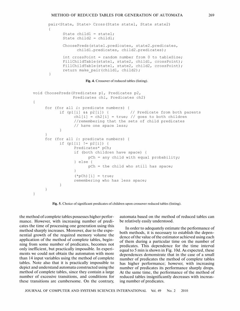
Algorithm 2. Crossover of reduced tables. The mainsteps of the crossover algorithm are shown in the listingin Fig. 4. Since parent chromosomes represented byreduced tables can have different sets of significantpredicates, first it is necessary to choose which of these

r

2 r

r

( )( )O g S Z X+ g

predicates will be present in child chromosomes. Thefunction ChoosePreds making this choice is shown inthe listing in Fig. 5. As a result of operation of thefunction ChoosePreds the predicates which are signifi�cant for both parents are inherited by both children,and each of the predicates present in just one parentspecimen goes to any of the children with equal prob�ability. The example of operation of the function forparent chromosomes shown in Fig. 6 is illustrated inFig. 7. After choosing significant predicates tables forboth children are formed. The filling algorithm isshown in the listing in Fig. 8. The illustration of theexample of filling the first row of the table of one of thechildren is shown in Fig. 9. In this implementation ofthe crossover operator, the values of each row of thechild table are influenced by the values of several rowsof the parent tables. In this case, the particular quan�tity placed in the cell of the child table is determinedby “voting” of all cells of parent tables which influencethis cell.

In the above variant of the algorithm, all automatonstates have the equal number of significant predicates( is the constant for the whole optimization process).However, the proposed crossover algorithm can easilybe extended to the case of the different number of sig�nificant predicates for the pair of parents.

r

x0

0

x1

1

x2

0

x3

1

x4

0

x5

0

x1

0

0

1

1

x3

0

1

0

1

s

0

1

0

2

z0

0

1

0

1

z1

0

0

1

1

z2

1

1

0

1

Fig. 1. State chromosome: reduced table (n = 6, r = 2).

x0

0

x1

1

x2

0

x3

1

x4

0

x5

0

0 1 0 0 1 0

1 − p p

Fig. 2. Example of mutation of the set of significant predi�cates.

268


POLIKARPOVA et al.

4. EXPERIMENTAL ESTIMATE OF THE METHOD OF REDUCED TABLES

For estimating the characteristics of the method ofreduced tables a number of experiments were per�formed in which this method was compared with therepresentation of control automata in the form ofcomplete tables of transitions and outputs [30]. Thecomparison was performed according to the followingcriteria: occupied memory volume, time spent for pro�cessing each generation, growth rate of the fitnessfunction (of the generation number and time).

It was already mentioned above that the method ofreduced tables solves the problem of exponentialgrowth of the size of automaton description withincreasing number of input variables (predicates of thecontrol object). This property of the method wasproved in the course of experimental verification. Dur�ing the experiment the automata descriptions werestored in the computer memory; therefore, the occu�pied memory volume in this case is proportional to the

size of the automaton description. The results ofexperiment are shown in Fig. 10a. It follows from theplot that the occupied memory volume in the case ofapplication of the complete tables exponentiallygrows, while for the method of reduced tables this vol�ume practically does not change with increasing num�ber of predicates. In reality it linearly depends on thenumber of predicates, however, the proportionalitycoefficient is so small that it is not observed in experi�ments. The dependence of time required for process�ing each generation on the number of predicates hasthe same character (Fig. 10b).

Now let us estimate the growth rate of the fitnessfunction. Figure 10c shows the dependences of thevalue of the estimator on the generation number forthe methods of complete and reduced tables (the mea�surements were performed for a small number of pred�icates). It follows from this plot that the optimizationusing the method of complete tables requires the cal�culation of a smaller number of generations. Thismeans that in the case of a small number of predicates

State Mutate(State state)

State mutant = state;

if (with the probability p) {

int from, to;

randomly choose from and to in such a way that

(mutant.predicates[from] == 1) && (mutant.predicates[to] == 0)

mutant.predicates[from] = 0;

mutant.predicates[to] = 1;

}

if (with the probability p1) {

mutant.table[i].targetState = random from 0 to nStates - 1;

}

if (with the probability p2) {

int nActsPresent = number of units in mutant[i].table.output;

if ((nActsPresent == 0) || (nActsPresent == nActions)) {

Index j = random number from 0 to nActions - 1;

mutant[i].table.output[j] = !mutant[i].table.output[j];

} else {

for (for all j: action numbers) {

mutant[i].table.output[j] = 1 with the probability

nActsPresent/nActions and 0 otherwise;

}

}

return mutant;

{

for (for all i: rows of table) {

}}

}

Fig. 3. Mutation of reduced tables (listing).



the method of complete tables possesses higher perfor�mance. However, with increasing number of predi�cates the time of processing one generation using thismethod sharply increases. Moreover, due to the expo�nential growth of the required memory volume theapplication of the method of complete tables, begin�ning from some number of predicates, becomes notonly inefficient, but practically impossible. In experi�ments we could not obtain the automaton with morethan 14 input variables using the method of completetables. Note also that it is practically impossible todepict and understand automata constructed using themethod of complete tables, since they contain a largenumber of excessive transitions, and conditions forthese transitions are cumbersome. On the contrary,

automata based on the method of reduced tables canbe relatively easily understood.

In order to adequately estimate the performance ofboth methods, it is necessary to establish the depen�dence of the value of the estimator achieved using eachof them during a particular time on the number ofpredicates. This dependence for the time intervalequal to 5 min is shown in Fig. 10d. As expected, thesedependences demonstrate that in the case of a smallnumber of predicates the method of complete tableshas higher performance; however, with increasingnumber of predicates its performance sharply drops.At the same time, the performance of the method ofreduced tables insignificantly decreases with increas�ing number of predicates.

pair<State, State> Cross(State statel, State state2)

{

State child1 = statel;State child2 = childl;

ChoosePreds(statel.predicates, state2.predicates, childl.predicates, child2.predicates);

int crossPoint = random number from 0 to tableSize;FillChildTable(statel, state2, childl, crossPoint); FillChildTable(statel, state2, child2, crossPoint);return make_pair(childl, child2);

Fig. 4. Crossover of reduced tables (listing).

void ChoosePreds(Predicates p1, Predicates p2,Predicates chl, Predicates ch2)

for (for all i: predicate numbers) {if (p1[i] && p2[i]) { // Predicate from both parents

chl[i] = ch2[i] = true; // goes to both children//remembering that the sets of child predicates

}}for (for all i: predicate numbers) {

if (pl[i] != p2[i]) {Predicates* pCh;

pCh = any child with equal probability;} else {

pCh = the child who still has space;}

(*pCh)[i] = true;remembering who has less space;

}}

{

// have one space less;

if (both children have space) {

}

Fig. 5. Choice of significant predicates of children upon crossover reduced tables (listing).

}

270


POLIKARPOVA et al.

The following conclusions can be made from theinvestigation of the characteristics of the methods ofcomplete and reduced tables:

(i) in the case of a small number of predicates theoptimization using the method of complete tablesrequires less time; however, thus constructed automataare incomprehensible;

(ii) beginning with a certain number of predicates,the application of the method of complete tables ispractically impossible, while the method of reducedtables yields rather good results with respect to therequired time and memory.

A tool based on the method described above wasdeveloped by us for automata generation [30, 31].

5. APPLICATION OF THE METHOD OF REDUCED TABLES FOR AUTOMATIC

CONTROL OF AN AIRCRAFT

The proposed method was applied to designing theautomatic control system for an aircraft model on ahigh level of abstraction. It is known that at presentautopilot systems are widely used in aircraft control;however, they do not provide a completely automaticflight. In particular, the switching between autopilotregimes and the adjustment of navigation devices isperformed manually. In this study the following taskwas formulated: to construct an aircraft controllingfinite automaton which completely automates theflight. In this case, the automaton can use the standardautopilot as the control object. The developed systemshould not produce nonstandard requirements to theground equipment.

5.1. Method of Generation of Aircraft Controlling Automaton

For solving the problem formulated above usinggenetic programming based on the method of reducedtables the following steps were made:

(i) choice of a spacecraft simulator;(ii) implementation of control object interface;(iii) determination of fitness function;(iv) construction of control automaton;(v) analysis of results of experiment.

5.2. Choice of a Spacecraft Simulator

In the considered problem, the control object is anaircraft which is situated in some medium, includingair (possibly, moving), runways, landscape, flight con�trol service, radio beacons, and so on. It is necessary toemulate aerodynamics, mechanics, and operation of

1

1

1

1

1 1/21/2

1

1

1

1

Fig. 7. Example of choosing significant predicates of chil�dren.

x1

0

0

1

1

x3

0

1

0

1

s

0

1

0

2

z0

0

1

0

1

z1

0

0

1

1

z2

1

1

0

1

x1

0

0

1

1

x3

0

1

0

1

s

1

2

2

0

z0

1

0

0

0

z1

1

0

1

1

z2

0

1

0

0

x0 x1 x2 x3 x4 x5

0 1 0 1 0 0

x0 x1 x2 x3 x4 x5

0 1 0 0 0 0

Fig. 6. Parent chromosomes represented as reduced tables.



Table 1. Input actions of automaton

Identifier Value description

x1 Aircraft is moving

x2 Aircraft velocity is sufficient for flying with extended flaps

x3 Aircraft velocity is sufficient for flying with retracted flaps

x4 Aircraft is flying

x5 Aircraft is near the ground

x6 Flight altitude corresponds to the recommended altitude level

x7 Aircraft is near the reference point of GPS receiver

void FillChildTable(State s1, State s2, States child, int crossPoint) { for (for all i: rows of table child) {

vector<int> linesl = choose rows of table s1 in which predicatessignificant for child have the same values as in row i,and if the predicate is significant for both parents and i >=crossPoint, its value is not taken into account;

vector<int> lines2 = choose rows of table s2 in which predicatessignificant for child have the same values as in row i,and if the predicate is significant for both parents and i <crossPoint, its value is not taken into account;

vector<Probability> p1(nStates);vector<Probability> р2(nStates);for (for all j from linesl) {

p1[target state for s1 in row j] += 1.0;}for (for all j from lines2) {

р2[target state for s2 in row j] += 1.0;

Divide values of p1 by the number of rows from linesl; Divide values of р2 by the number of rows from lines2; vector<Probability> р = p1 + р2;child[i].targetState = random with probability distribution р;for (for all k: action numbers) {

Probability ql, q2;for (for all j from linesl) {

ql += s1[j].output[k];

for (for all j from lines2) {

Divide ql by the number of rows from linesl;Divide q2 by the number of rows from lines2;child[i].output[k] = 1 with the probability (ql + q2)/2

}

}

}

q2 += s2[j].output[k];}

}}

Fig. 8. Filling tables of children for crossover of reduced tables (listing).

the aircraft equipment. Since it is rather cumbersometo develop the necessary emulator, it is natural to use aready emulator. For this purpose the aviation simula�tor X�Plane [32] was chosen; the specific features of

this simulator are the precision of physical simulationand documented interface of interaction with otherprograms (API), which made it possible to use thissimulator in the experiment.

and 0 otherwise;

272


POLIKARPOVA et al.

5.3. Choice of Control Object Interface

The simulator X�Plane provides getting from theaircraft and transmitting to the aircraft of a large num�ber of data. In this experiment, it was impossible to useall these data in the control automaton, since in thiscase the optimization process would be too long. It wasalready mentioned above that the realistic character ofthe proposed method of generation of control autom�ata is provided by the high level of abstraction of thelogics. In this case, predicates and actions of the con�trol object are manually chosen and implemented.

In the studied problem 7 input (Table 1) and24 output variables (Table 2) were used; we assumedthat this amount was sufficient for the aircraft controlon a high level of abstraction. For each of the chosenvariables the subprogram corresponding to the predi�cate or action of the control object was developed.

These subprograms interact with the spacecraft simu�lator, reading the device indications and acting on thecontrol organs of the aircraft. The composition ofdevices and control organs is shown in Fig. 11.

5.4. Fitness Function

Let us reformulate the problem in the form of thefitness function. The autopilot should guide the air�craft along the route and not crash it. Therefore, twoimportant factors can be separated: deviation from theroute and the aircraft safety. It is also important thatafter passing along the route the aircraft should stop(or decelerate to a safe velocity) on the runway. Thecombined deviation from the route both with respectto position and velocity is calculated in the form of thetime integrals of the absolute values of correspondingdeviations,

x1

0

0

x3

0

1

s

0

1

z0

0

1

z1

0

0

z2

1

1

x0 x1

0 0

0

1

2

0.5

0.5

0

0

1

2

0

0.5

0.5

0.5 0 1

z0 z1 z2

0.5 0.5 0.5

z0 z1 z2

0.5 0.5 0.5

z0 z1 z2

0.5 0.25 0.75

x0

0

0

x1

0

0

s

2

1

z0

0

1

z1

0

1

z2

1

0

x0 x1 x2 z0 z1 z2

0 0 1 1 0 1

0

1

2

0.25

0.5

0.25

s

10.5 1 − 0.25 0.75

0.5

Corresponding rows in the

Corresponding rows in thetable of the second parent

(the value x1 is not taken into account, since the row number < crossPoint)

table of the first parent

Fig. 9. Example of filling the row of the child table upon crossover of reduced tables.



,

where is the combined deviation from the route withrespect to position, , is the time of beginning of theemulation, is the time of the end of emulation, and

is the position deviation at the time instant ;

,

( )1

0

t

t

P p t dt= ∫P

0t

1t( )p t t

( )1

0

t

t

V t dt= ∫v

where is the combined deviation from the optimalvelocity and is the deviation from the optimal

velocity at the time instant . Let us denote by , ,and the weighting coefficients of a crash, position,and velocity deviations. The coefficients determinethe relative importance of the corresponding defects ofthe autopilot behavior. The following values weretaken for these coefficients: , P

α = 0.01 1/m,

and Vα = 0.01 s/m. As a result, we chose the fitness

function of the form

V( )tv

t Cα

Pα

Vα

9Cα=

1400

1

1200

1000

800

600

400

200

02 3 4 5 6 7 8 9 10

Number of predicates

1

2

Necessary memory volume, MB(a)

250

1

200

150

100

50

02 3 4 5 6 7 8 9 10


1

2

Time required for generation processing, s

(b)

1.2

1.0

0.8

0.6

0.4

0.2

0

1

2

Estimator value(c)

117

3349

6581

9713

129145

161177

193209

225241

257273

289

Generation number

1.2

1

1.0

0.8

0.6

0.4

0.2

02 3 4 5 6 7 8 9 10


1

2

Fitness value achieved for 5 min(d)

Fig. 10. The dependence of the memory amount (a), the processing time of generation (b). The value of estimation function forthe given duration of the method (d) on the number of predicates and the value of estimation function on the number of genera�tion (c); 1—full tables, 2—reduced tables.

274


POLIKARPOVA et al.

,

where is the variable which is equal to zero if the air�

craft is safe, and unity if it is broken; = 77 s is the timeduring which in the case of exact following the route(which is physically impossible) autopilot would getthe same value of the fitness function as the “ideal”physically possible autopilot gets during the wholeflight. The function is normalized to the interval (0, 1),as compared with the “ideal” autopilot. Thus, if the

( )

1 0

1 0

1 1i

t tfPP VVt bC

t tα α

α

−=

⎛ ⎞++ +⎜ ⎟−⎝ ⎠

b

it

function is equal to unity, this means that the goal ofoptimization has been achieved.

5.5. Construction of Control Automaton

The algorithm of construction of the controlautomaton consists of the following steps:

(1) initial population of automata is generated in arandom way;

(2) each automaton in the population is estimated.For this purpose, the flight is simulated in the space�craft simulator controlled by the estimated automa�ton, and the data on the route and state of the aircraft

Air velocity indicatorx1, x2, x3

Altimeterx4, x5, x6

ALT�Constant altitude regimez8

V/S�Constant vertical velocity regimez9

HFG�Regime of flight along the coursez6

LOC�Regime of flight toward a pointz5

G/S Descent using a beaconz7

Climb ratez22

Flight altitudez22

Autopilot

Navigationreceiver NAV1z1, z2

GPS receiver

Distance to the targetx7

Reference pointz3

Flap controlhandlez15, z16, z17

Throttlez12, z13, z14

Flight controlz4

Landing gear extension handlez18, z19

Wheel brakez10, z11

Source of signal of indicator of horizontal situationz20, z11

HSI�Indicatorof horizontal

situation

Fig. 11. Applied devices and control organs of the aircraft.



are recorded. Then the value of the fitness function iscalculated based on these data;

(3) if there is one automaton with the fitness func�tion equal to unity in the population it is chosen as theresult, and the process of optimization is completed;

(4) in the opposite case, a new generation is con�structed using the operators of mutation and cross�over; after that the process returns to step 2.

The plot of variation of the fitness function withincreasing generation number in the course of opera�tion of the above algorithm is shown in Fig. 12. Themaximal value of the estimator equal to unity for twolast generations testifies the successful completion ofthe process of optimization.

The constraint on the number of significant predi�cates in each state r = 1 was imposed upon the autom�aton generation. Even for this constraint the optimiza�tion lasted about one month. Note that most of thetime was spent for the calculation of the fitness func�tion: the emulation necessary for estimation of oneautomaton required about 5 min. The automatonobtained as a result of optimization has a small num�ber of states and transitions. However, it is rather com�plicated for comprehension due to a large number ofactions at transitions. In order to simplify the automa�ton, the actions rejecting each other, which do not

influence the aircraft behavior in this state, were man�ually eliminated. The automaton states were enumer�ated and named. The final variant of the automaton isshown in Fig. 13. Since the number of significantpredicates in each state of the control automaton was

1.0

1

0.8

0.6

0.4

0.2

07 13 19 25 31 37 55 97103

Generation

Fitness

9185797367614943

1.2

Fig. 12. Variation of fitness in the course of evolution.

Table 2. Output actions of automaton

Identifier Action description

z1 Adjusting navigation receiver to the frequency of landing beacon of the departure airportz2 Adjusting navigation receiver to the frequency of landing beacon of the destination airportz3 Switching the GPS receiver in the following regime to the reference pointz4 Switching the flight control switch into the position “AUTO”z5 Switching autopilot to the flight regime to the point in the horizontal planez6 Switching autopilot to the flight regime along the course in the horizontal planez7 Switching autopilot to the descent regime using the beaconz8 Switching autopilot to the constant altitude regimez9 Switching autopilot to the constant vertical velocity regimez10 Switching on wheel brakez11 Switching off wheel brakez12 Setting maximal fuel supplyz13 Setting intermediate fuel supplyz14 Setting minimal fuel supplyz15 Retracting flapsz16 Setting flaps into takeoff positionz17 Setting flaps into descent positionz18 Extending landing gearz19 Retracting landing gearz20 Using navigation receiver as the source of signal of indicator of horizontal situationz21 Using GPS receiver as the source of signal of indicator of horizontal situationz22 Setting climb rate and flight altitude for autopilotz23 Controlling rudder according to autopilot signalsz24 Setting rudder into the central position

276


POLIKARPOVA et al.

0. Start

1. Acceleration

2. Leaving the ground

3. Climb to safe

4. Flight using

5. Adjustment of 6. Landing approach

7. Descent

8. Landing

9. Deceleration

10. Not used

!x7/z: 1, 3, 5, 11, 15, 18, 20, 22, 23

x2/z: 3, 4, 5, 9, 12, 16, 23

x3/z: 15, 19, 24

!x7/z:5, 21

x7/z: 2, 6, 7, 13, 20

x7/z: 5, 7

!x7/z: 5, 7, 9, 21 ,23!x6/z: 14, 17, 18

x5/z8

!x4/z10

x5

!x3/z23

x1/z23

!x2/z: 3, 4, 5, 12, 23

x7/z: 2, 3, 4, 5, 9, 11, 14, 16, 19, 21 ,22 ,24

!x7

!x5

x4

x6

!x1/z15

altitude

GPS navigator

landing approach

Fig. 13. Transition graph of the obtained automaton.

taken equal to unity, not more than two transitionsfrom each state were possible. Due to the fact that thepredicates and actions of the control object were chosenon a rather high level of abstraction, the automaton withsuch a simple structure was sufficient for control.

The automaton shown in Fig. 13 can be rather eas�ily heuristically (without the use of genetic program�ming) constructed. For example, in [33] a very similartransition graph describing the aircraft flight (Fig. 14a)was given as the example of the state diagram. In

Fig. 14b the states and transitions of this automatonare correlated with the states and transitions of theautomaton obtained using genetic optimization in thispaper. The difference between the two transitiongraphs is explained by the difference in the problemformulation. However, often it is not easy to constructthe control automaton manually. This automaton inmost cases is nonoptimal and unjustified complex.Besides, the optimization approach is characterizedby better scalability.

Fig. 14. (a) State diagram for the aircraft flight [33] and (b) its comparison with automatically constructed automaton.



Is transported Stays

Taxing

Taxing

On the ground

Ready for takeoff

Takeoff

Deceleration

Continue

Cancel

Climb

Motion with

Descent

In air

In flight

Approaches

Aircraft

Wheels

Cancel

Free for takeoff

0. Start

Ready for takeoff

1. Acceleration

2. Leaving ground

9. Deceleration

Deceleration

Takeoff

7. Descent

8. Landing

Descent

6. Approach landing

5. Adjustment of turn

4. Flight to reference

velocity

cruising

Motion with

3. Climb to minimal

Climb

On runway In air

!x7

x3

Cancel

!x4

!x6

!x7

x2

x5 Cancel

x7

x7

!x5

Ready to taxi

Ready to taxi

On runway

leavingground

cruisingvelocity

groundLandingLeaves runway

(a)

(b)

(with flaps)

point

altitude (without flaps)

278


POLIKARPOVA et al.

(a)

10.Not used

0. Stop

1. Acceleration

2. Leaving ground

3. Takingsafe

altitude

4. Flight acco�rding to GPS

navigator

5. Adjustmentof

landing

6. Landing

7. Descent

8. Landing

9. Decelera�tion

(b)

10.Not used

0. Stop

1. Acceleration

2. Leaving ground

3. Takingsafe

altitude


navigator

5. Adjustmentof

landing

6. Landing

7. Descent

8. Landing

9. Decelera�tion

(c)

10.Not used

0. Stop

1. Acceleration

2. Leaving ground

3. Takingsafe

altitude


navigator

5. Adjustmentof

landing

6. Landing

7. Descent

8. Landing

9. Decelera�tion

(d)

10.Not used

0. Stop

1. Acceleration

2. Leaving ground

3. Takingsafe

altitude


navigator

5. Adjustmentof

landing

6. Landing

7. Descent

8. Landing

9. Decelera�tion

Fig. 15. Automaton and aircraft in different states: (a) acceleration; (b) leaving ground; (c) climb to safe altitude; (d) flight usingGPS navigator; (e) adjustment of landing approach; (f) landing approach; (g) descent; (h) landing; (i) deceleration.



(e)

10.Not used

0. Stop

1. Acceleration

2. Leaving ground

3. Takingsafe

altitude


navigator

5. Adjustmentof

landing

6. Landing

7. Descent

8. Landing

9. Decelera�tion

(f)

10.Not used

0. Stop

1. Acceleration

2. Leaving ground

3. Takingsafe

altitude


navigator

5. Adjustmentof

landing

6. Landing

7. Descent

8. Landing

9. Decelera�tion

(g)

10.Not used

0. Stop

1. Acceleration

2. Leaving ground

3. Takingsafe

altitude


navigator

5. Adjustmentof

landing

6. Landing

7. Descent

8. Landing

9. Decelera�tion

(h)

10.Not used

0. Stop

1. Acceleration

2. Leaving ground

3. Takingsafe

altitude


navigator

5. Adjustmentof

landing

6. Landing

7. Descent

8. Landing

9. Decelera�tion

Fig. 15. (Contd.)

280


POLIKARPOVA et al.

5.6. Analysis of Results of Experiment

When the optimization is completed, the test emu�lation of the flight controlled by the constructed opti�mal automaton was performed. Figure 15 shows theautomaton, the aircraft position, and the device indi�cations at different stages of test emulation. In thecourse of test emulation the deviation from the routeand the recommended velocity, the flight altitude(which makes it possible to determine the timeinstants of leaving the ground and touching theground), and the acting overloads were recorded. Therecorded data are shown in Fig. 16.

It follows from the plot that the maximal deviationof the aircraft from the route during the whole flighttime was 314 m. It did not exceed 60 m during thewhole flight except for a 1 min segment in the middleof the plot when the deviation is the least critical. Thetime instants of leaving and touching the ground canbe determined from the plot of the flight altitude:35 and 271 s, respectively. It follows from the estab�lished time and the plot of deviation from the routethat the maximal deviation during acceleration was12 m, and during deceleration 10 m. The deviationswhich are significant but do not go beyond the runwaysprovide the conclusion that the generated automatonguided the aircraft along the route with sufficient pre�cision.

(i)

10.Not used

0. Stop

1. Acceleration

2. Leaving ground

3. Takingsafe

altitude


navigator

5. Adjustmentof

landing

6. Landing

7. Descent

8. Landing

9. Decelera�tion

Fig. 15. (Contd.)

0

(a)

114

2740

5366

7992

105118

131144

157170

183196

209222

235248

261274

287300

50

100

150

200

250

300

350

Time, s

Deviation from the route, m

0

(c)

114

2740

5366

7992

105118

131144

157170

183196

209222

235248

261274

287300

50

100

150

200

250

300

350

Time, s

0

(d)

114

2740

5366

7992

105118

131144

157170

183196

209222

235248

261274

287300

0.40.60.81.01.21.41.6

Time, s

0.2

�5

(b)

113

2537

4961

7385

97109

121133

145157

169181

193205

217229

241253

265277

0

5

10

15

20

25

Time, s

289

Velocity deviation, m/s

Altitude above sea level, m Overload, g

Fig. 16. Results of testing: (a) deviation from the route; (b) deviation from the recommended velocity; (c) flight altitude above thesea level; (d) overload.



It follows from the plot of recommended velocitythat the velocity regime was observed, except forexceeding the velocity by 20.34 m/s at the time instantof touching the ground, which was compensated in thecourse of deceleration and did not result in a consider�able excess in the stopping distance. The combineddeviation of the aircraft position after stopping includ�ing the transverse deviation from the center of the run�way and the excessive stopping distance is 6.5 m. It fol�lows from the plot of overload that the enhanceddeceleration did not result in a considerable discom�fort of passengers. This analysis yields the conclusionon the satisfactory quality of the automatically con�structed automaton.

CONCLUSIONS

The disadvantages of the existing methods of gen�eration of finite automata using genetic algorithmswere demonstrated and the method free from thesedisadvantages was proposed. The performance of theproposed method and its memory requirements wereexperimentally estimated. The method was success�fully tested in the problem of automatic generation ofthe aircraft control system and proved its applicabilityfor solution of practical tasks.

REFERENCES

1. V. M. Kureichik, “Genetic Algorithms: State of the Art,Problems, and Perspectives”, Izv. Ross. Akad. Nauk,Izv. Ross. Akad. Nauk, Teor. Sist. Upr., No. 1, 144–160(1999) [Comp. Syst. Sci. 38 (1), 137–152 (1999)].

2. V.V. Kureichik, V.M. Kureichik, and P.V. Sorokoletov,“Analysis and a Survey of Evolutionary Models”, Izv.Ross. Akad. Nauk, Izv. Ross. Akad. Nauk, Teor. Sist.Upr., No. 5, 114–126 (2007) [Comp. Syst. Sci. 46 (5),779–791 (2007)].

3. J. R. Koza, Genetic Programming: On the Programmingof Computers by Means of Natural Selection (MIT Press,1992).

4. V. M. Kureichik and S. I. Rodzin, “Evolutionary Algo�rithms: Genetic Programming”, Izv. Ross. Akad.Nauk, Izv. Ross. Akad. Nauk, Teor. Sist. Upr., No. 1,127–137 (2002) [Comp. Syst. Sci. 41 (1), 123–132(2002)].

5. E. M. Gold, “Language Identification in the Limit”,Informat. Control, 10, 447–474(1967).

6. A. Belz, “Computational Learning of Finite�StateModels for Natural Language Processing”, PhD thesis,University of Sussex, 2000.

7. C. H. Clelland and D. A. Newlands, “Pfsa Modelling ofBehavioural Sequences by Evolutionary Program�ming”, in Proceedings of 2nd Australian Conf. on Com�plex Systems Complex’94, Rockhampton, Queensland,Australia, 1994, 165–172.

8. S. Das and M.C. Mozer, “A Unified Gradient�Descent/Clustering Architecture for Finite StateMachine Induction”, Advances in Neural InformationProcessing Systems, 6 (1994).

9. M. M. Lankhorst, “A Genetic Algorithm for the Induc�tion of Nondeterministic Pushdown Automata”, Com�puting Science Report (University of CroningenDepartment of Computing Science, Groningen, 1995).

10. A. Belz and B. Eskikaya, “A Genetic Algorithm forFinite State Automata Induction with an Application toPhonotactics”, in Proceedings of ESSLLI�98 Workshopon Automated Acquisition of Syntax and Parsing, Saar�bruecken, Germany, 1998, 9–17.

11. D. Ashlock, A. Wittrock, and T.�J. Wen, “TrainingFinite State Machines to Improve PCR PrimerDesign”, in Proceedings of Congress on EvolutionaryComputation (CEC’02), Honolulu, Hawaii, USA, 2002,13–18.

12. D. A. Ashlock, S. J. Emrich, K. M. Bryden, et al.,“A Comparison of Evolved Finite State Classifiers andInterpolated Markov Models for Improving PCRPrimer Design”, in Proceedings of 2004 IEEE Sympo�sium on Computational Intelligence in Bioinformatics andComputational Biology (CIBCB’04), Jolla, California,USA, 2004, 190–197.

13. S. M. Lucas, “Evolving Finite State Transducers: SomeInitial Explorations”, in Proceedings of Genetic Pro�gramming: 6th European Conference (EuroGPKh03)(Springer, Berlin, 2003), 130–141.

14. P. G. Lobanov and A. A. Shalyto, “Application ofGenetic Algorithms for Automatic Construction ofFinite�State Automata in the Problem of Flibs”, Izv.Ross. Akad. Nauk, Izv. Ross. Akad. Nauk, Teor. Sist.Upr., No. 5, 127–136 (2007) [Comp. Syst. Sci. 46 (5),792–801 (2007)].

15. F. N. Tsarev and A. A. Shalyto, “Application of GeneticAlgorithms for Construction of Automatons with Min�imal Number of States for the “Smart Ant” Problem”,in Scientific Software in Education and ScientificResearch (SPbGU PU, St. Petersburg, 2008), 209–215.

16. A. Teller, and M. Veloso, PADO: A New Learning Archi�tecture for Object Recognition. Symbolic Visual Learning(Oxford Univ. Press, New York, 1996).

17. W. Banzhaf, P. Nordin, R. E. Keller, et al., Genetic Pro�gramming � An Introduction. On the Automatic Evolutionof Computer Programs and its Application (MorganKaufmann Publishers, San Francisco, 1998).

18. W. Kantschik, P. Dittrich, and M. Brameier, “Empiri�cal Analysis of Different Levels of Meta�Evolution”, inProceedings of Congress on Evolutionary Computation,,Washington DC, USA, 1999.

19. W. Kantschik, P. Dittrich, M. Brameier, et al., “Meta�Evolution in Graph GP”, in Proceedings of Genetic Pro�gramming: Second European Workshop (EuroGP’99),Goeteborg, Sweden, 1999.

20. A. Teller and M. Veloso, “Internal Reinforcement in aConnectionist Genetic Programming Approach”, inArtificial Intelligence (North�Holland Pub. Co, 1970),161.

21. J. H. Miller, “The Coevolution of Automata in theRepeated Prisoner’s Dilemma. Working Paper” (SantaFe Institute, 1989).

22. W. M. Spears and D. F. Gordon, “Evolving Finite�StateMachine Strategies for Protecting Resources”, in Pro�ceedings of International Syposium on Methodologies for

282


POLIKARPOVA et al.

Intelligent Systems, Charlotte, North Carolina, USA,2000.

23. D. Ashlock, Evolutionary Computation for Modeling andOptimization (Springer, New York, 2006).

24. C. Frey and G. Leugering, “Evolving Strategies forGlobal Optimization. A Finite State MachineApproach”, in Proceedings of Genetic and EvolutionaryComputation Conference (GECCO�2001), San Fran�cisco, USA, 2001), 27–33.

25. P. Petrovic, “Simulated Evolution of Distributed FSABehaviour�Based Arbitration”, in Proceedings of EighthScandinavian Conference on Artificial Intelligence(SCAI'03), Bergen, Norway, 2003.

26. P. Petrovic, Evolving Automatons for Distributed Behav�ior Arbitration. Technical Report (Norwegian Universityof Science and Technology, Trondheim, Norway, 2005).

27. P. Petrovic, Comparing Finite�State Automata Represen�tation with GP�trees. Technical report (Norwegian Uni�versity of Science and Technology, Trondheim, Norway,2006).

28. N. I. Polikarpova and A. A. Shalyto, Automaton Pro�gramming (Piter, St. Petersburg, 2009) [in Russian].

29. J.R. Koza, Future Work and Practical Applications ofGenetic Programming. Handbook of Evolutionary Com�putation (IOP Publishing Ltd, Bristol, 1997).

30. N. I. Polikarpova, V. N. Tochilin, and A. A. Shalyto,“Application of Genetic Programming for Implemen�tation of Systems with Complex Behavior”, in Proceed�ings of 4th International Scientific–Practical Conferenceon Integrated Models and Soft Calculations in ArtificialIntelligence, vol. 2 (Fizmatlit, Moscow, 2007), 598–604.

31. N. I. Polikarpova, V. N. Tochilin, and A. A. Shalyto,“Development of a Library for Generation of ControlAutomata Using Genetic Programming”, in Proceed�ings of 10th International Conference on Soft Calculationsand Measurements, vol. 2 (SPbGETU “LETI”, St. Peters�burg, 2007).

32. http://www.x�plane.com/.33. E. Hull, K. Jackson, and J. Dick, Requirements Engi�

neering (Springer, Berlin, 2002).

method of reduced tables for generation of …is.ifmo.ru/articles_en/_polikarpova_samolet.pdfjournal...

Documents