NASA Technical Paper 1753

Method for .Estimating Crack- Extension Resistance Curve From Residual-Strength Data

Thomas W. Orange. ..

NOVEMBER 1980

,

\

https://ntrs.nasa.gov/search.jsp?R=19810002909 2018-08-26T00:13:49+00:00Z

I’ TECH LIBRARY KAFB, NM

NASA Technical Paper 1753

Method for Estimating Crack- Extension Resistance Curve From Residual-Strength Data

Thomas W. Orange Lewis Research Center Cleveland, Ohio

National Aeronautics and Space Administration

Scientific and Technical Information Branch

1980

Summary This report presents a method for estimating the

crack-extension resistance curve (R-curve) from residual-strength (maximum load against initial crack length) data for precracked fracture specimens. The method allows additional information to be inferred from simple test results, and that information can be used to estimate the failure loads of more complicated structures of the same material and thickness.

The analytical basis for the method was developed by the author in a previous report. Numerical differentiation of the residual-strength data is re- quired, and the problems that it may present are discussed. The method is demonstrated and verified by using various types of residual-strength data from the literature.

Introduction This report presents a method for estimating the

crack-extension resistance curve (R-curve) from residual-strength (maximum load against original crack length) data for precracked fracture specimens. Such data may be found in the literature or may exist in company files. The method allows additional information to be inferred from simple test results, and that information can be used to estimate the failure loads of more complicated structures (such as reinforced panels) of the same material and thickness.

The progressive development of the R-curve concept has been reviewed in reference 1. The concept postulates that, for a given material and thickness, there is a unique relationship between the amount of stable crack growth under rising load and the crack-tip stress intensity factor. The relationship is called the crack-extension resistance curve, or R-curve, and represents the response of the material near the crack tip to externally imposed loading. If the R-curve is known, both failure load and critical crack length can be predicted (as functions of initial crack length) for any specimen or structural configuration for which an appropriate stress intensity analysis is available. For example, refer- ence 2 illustrates the use of the R-curve to predict the failure load for a strap-reinforced panel. Current methods for determining the R-curve (ref. 3) require that the specimen be instrumented to measure crack

opening displacement, and the Rcurve is derived from the load-displacement record.

The analytical foundation for the present report is developed in reference 4. That report examines several semiempirical fracture analyses that attempt to relate maximum load to initial crack length in terms of one or two empirical parameters. It showed that an R-curve can be developed that is mathematically equivalent to any one of the semi- empirical analyses. In the present report the R-curve is developed directly from residual-strength data without recourse to any semiempirical analysis.

This report first reviews some characteristics of the R-curve concept when applied to practical test specimens. Next the method for generating an esti- mated R-curve is derived. Numerical differentiation of the residual-strength data is required, and the problems that it may present are discussed. Finally R-curves are estimated for several materials by using data from the literature.

Symbols length of single-tip crack or half-length of double-tip crack

effective modulus, E for plane stress or E / ( l - u 2 ) for plane strain, where E is Young's modulus and Y is Poisson's ratio

strain energy release rate fracture toughness, GA or GR at instability

crack extension resistance opening-mode stress intensity factor number of crack tips (one or two) specimen width stress intensity calibration factor, K r / u f i sensitivity factor (eq. (1)) sensitivity factor (eq. ( 5 ) ) effective crack extension (sum of physical

condition

crack extension plus a plastic zone correction)

relative crack length, na/W stress normal to crack ultimate tensile strength yield strength

Subscripts: C at critical or instability condition 0 initial value (before loading)

R-Curve Concept The R-curve concept is illustrated schematically in

figure 1 €or an infinite body containing a crack whose original length is 2ao. The strain energy release rate is given by

m d represents the driving force (per unit thickness) tending to cause crack propagation. The material’s resistance to crack propagation GR is a function of crack extension A. In R-curve analysis the subscripts A, R , and c are customarily used to denote applied and resisting forces and critical values, respectively. The R-curve is located with its origin at a=ao. As stress normal to the crack is applied and increased to 90 percent of the subsequent critical stress in figure 1, the crack must extend only a small distance to develop a large resistance. At this point the crack- extension resistance equals the driving force, and the crack is stable. As the stress is increased.

GC-. /

Crack length, a

Figure L - Schematic representation of R-curve in- stability concept for an infinite body.

progressively larger amounts of crack extension are required to resist the crack driving force. Finally at the critical stress uc the driving-force curve and the R-curve are tangent. Beyond the point of tangency the driving force increases faster with crack length than does the material’s resistance. This instability condition represents the failure of the body. The point of tangency defines the fracture toughness G , and the critical crack length 2a,. Since the driving- force curve for an infinite body is a straight line, it should be apparent that both the fracture toughness G , and the amount of crack extension at instability A, increase with increasing original crack length 2ao. If the R-curve exhibits a plateau, G, and A, may asymptotically approach limit values.

Instability Calculations

In simple finite bodies and test specimens the presence of stress-free boundaries results in an additional increase in the crack driving force as the crack extends toward a boundary. Thus the slope of the driving-force curve increases continuously with increasing crack length. The instability condition for a typical finite-width specimen is shown in figure 2 and is determined as follows. For a given specimen configuration and loading the dimensionless stress intensity calibration factor is defined as

Y E 3 =fcn(h) &

where K I is the opening-mode elastic stress intensity factor, h=na/ W is the relative crack length, and n is the number of crack tips (one or two). If we define a dimensionless sensitivity factor as

a0 ac Crack length. a

Figure 2 - R-curve instability concept for a finite body.

2

then (for constant stress) the crack driving-force curve and its slope are

E'GA = *u2a

E' - = pu2(1 +2a) dGA da

For convenience the crack-extension resistance curve and its slope are written here as

g(A) =E' GR

g ' (A) =E' - dGR dA

At the instabi l i ty point , G A = G R and dGA/da=dGR/dA (fig. 2 ) . If g ( A ) and g ' (A) are mathematically describable, the instability point is determined by the simultaneous solution of the following equations:

E'G, = Y:u:(ao + A , ) =g(A , ) (2)

E ' E ( = Y:u,"(l +2ac)=g' (A, ) da (I,

The coefficients Y and CY are usually expressed as trigonometric or polynomial functions of the relative crack length X. As a result a closed-form simultaneous solution is seldom possible, and numerical methods must be used to solve for A,. This can be done as follows: Dividing equation (3) by equation (2) and rearranging terms give

If the functions g(A) and g'(A) and the appropriate equation for CY are substituted into equation (4), then, for prescribed values of a0 and W, A, is the least positive root of equation (4). This root can be found by any of several numerical methods. Next, the function g(A) is evaluated at A, to calculate g(A,). Finally the fracture stress u, is obtained from

equation (2) by using the appropriate value of Y,. In this report the expression

Y = (?r secant - ) 7FX 112 2

is used for the center-crack specimen (ref. 5) .

Instability in Finite Bodies

For a crack in an infinite body both G, and A, increase with increasing initial crack length. In a finite body as the initial crack length is increased from zero, G , and A, increase at first. However, because dY/& continually increases with X, both G, and A , reach maximum values that depend on the specimen width W and the forms of both the driving- force curve and the R-curve. As the initial crack length is increased still further, both G, and A, begin to decrease. This behavior is shown schematically in figure 3, where instability curves are shown for a wide range of initial crack lengths. The locus of all instability points is shown by the dashed line.

It is useful to define a sensitivity factor

which is shown for the center-crack specimen in figure 4. For comparison, y is also shown for the standard compact (tension) specimen. This was derived by using the expression

Y=h"/2(1 - q 3 l 2 ( 2 + X)(0.886 + 4.64 X

- 13.32 X2 + 14.72X3 -5.6 X4)

L Locus of

Relative crack length, A

Figure 3. - R-curve instability for a wide range of initial crack lengths,

3

111111 I I

20 -

16 -

L' 12- 2- - 0

m U c

.- c > .- .- - 8-

VI

4 -

0.4705

I 0 .2 . 4 . 6 .8 LO

Relative crack length, A

Figure 4 - Sensitivity factor for center-crack and com- pact specimens.

from reference 6. Note that the function X has a minimum value. Then for a given specimen width the first term in equation (4) must also have a minimum value. In graphical terms this means that if, at a given point, the R-curve's slope is too low or its magnitude too high or both, a driving-force ( G A ) curve cannot be both coincident and tangent at that point. Thus for a given specimen width the value of X at ymin defines the critical crack length at which both crack extension A, and fracture toughness G , or Kc are maximum. Note that both ymin and the relative crack length at which it occurs are different for different specimen types. The fact that the function y has a minimum has additional significance that is evident later in this report.

Comments

Although the subject has received scant attention in the literature, it is possible to estimate the R-curve from residual-strength data by using purely graphical methods. The method is shown in figure 5 . To simplify the illustration, assume that we know the residual strengths of four specimens having the same initial crack length but different widths. Construct a driving-force (GA) curve for each specimen by using residual strength in the equation following equa- tion (1). Then draw the estimated R-curve from the point (a =uo, GA = 0) in such a way that it is tangent

I Y U

V E

a0 Crack length, a

Figure 5. - Example of graphical method for estimating R- curve from residual-strength data. (W4 < Wj < W2 < W1 =

00; 0 4 < 0 3 < 0 2 < 0 1 )

at some point to each of the driving-force curves. If initial crack lengths are not constant, it is convenient to let the x-axis be given by crack extension A. Then each driving-force curve begins at a distance uo to the left of the origin. Although the procedure appears simple, in practice it is tedious and subjective at best. If significant data scatter exists, one's skill with the French curve will be severely tested.

In concluding this section it should be emphasized that, in this report, A is the effective crack extension. It is the sum of the physical crack extension plus an adjustment to account for the effect of crack-tip plasticity. The nature of the plasticity adjustment, although technically significant, has no influence on the analyses and conclusions in this report.

Analysis The analytical foundation for this report was

developed in reference 4. However, the common elements of the derivation are repeated here for con- venience. In the preceding section it was shown that, if a mathematical formulation for the R-curve is available, fracture stress can be predicted as a function of original crack length. In this section i t is shown that, if proper estimates of residual strength and its first derivative can be made, the R-curve can be estimated.

The first step requires that we differentiate equation (2) with respect to A,, and that operation requires some prior consideration. For a given spec- imen type there are many combinations of specimen width and initial crack length that will result in instability at the same point on the R-curve, and each combination has an associated fracture stress. To cause a small change dA, in the instability point, there must be a change in the specimen width or the

4

initial crack length or both, and there will be a change in the fracture stress. Thus, when differentiating equation (2), the terms W, u, and a0 are treated as variables.

Differentiating both sides of equation (2) with respect to A, yields

d dAc - E'G, = Y,u,~cY, 2 2

da0 ao+A, d W +1- -

Then equation (6) becomes

and, since dao/dA, #O, we have

Case ZZ: ao/W=Constant [dW =(W/ao)dao].- Now assume that there is a function h such that

h(a0) = (I, 2 l

and substituting equation (3) results in

Now equation (6) becomes

o=u: [ 2 (1 +2a,) - r -.

and since dao/dA, #O, we have

At this point it is helpful to reduce the problem to one of a single independent variable by prescribing Case ZZZ: a0 = Constant (dao = O).-This case is of the manner in which a0 and Wmay vary. Three cases limited usefulness but is included for completeness. are considered. Assume that there is a function j such that

there is a function f such that we can define Case Z: W = Constant (dW = O).-Assume that

A

Now equation (6) becomes

0 = - (a0 + A,)[ - %j(W) + j ’ ( W)] d W dAC

and since d W/dA, # 0 and (a0 +A,) # 0,

In reference 4 the functions f, h, or j and their derivatives were obtained from analytical formulations presented in various semiempirical fracture analyses. However, if sufficient and suitable experimental data are available, these functions and derivatives can be obtained directly from the data by curve fitting and numerical differentiation. Then the fitted function and its derivative are used to determine the corresponding R-curve as follows: First, at a given point on the residual-strength curve, the functionf, h, o r j and its derivative are estimated by using suitable numerical methods (discussed later). Second, the function and its derivative are substituted into the appropriate version of equation (7), which must be solved for A,. A numerical solution is usually required, and in this report a standard program for a desktop calculator was used, with A , always taken as the least positive root. Finally A, and the fitted value of 0: (which equalsf, h, or J] are substituted into equation (2) to calculate E’G, . The resulting pair (E’Gc,Ac) define a point (E’GR ,A) on the R-curve. The process is repeated at additional points on the residual-strength curve. If desired, the R-curve can be expressed in terms of K R ’ ( E ’ G R ) ” ~ . Also, a suitable function can be fit to describe GR or KR as an explicit function of A.

At best this estimation method has the same limitation as a standard R-curve test run under load control; namely, for a given specimen the R-curve can only be measured (or estimated) to the point at which the crack becomes unstable. Furthermore the extent to which the R-curve can be estimated may depend on the shape of the actual R-curve, the nature of the residual-strength data, or both. For example, suppose that the actual R-curve has a pronounced knee (typical of high-strength, low-toughness materials), as shown in figure 3. There, as the initial crack length increases from 0.2 W to 0.8 W, the location of the instability point on the R-curve moves only a small distance. Thus, even if one had many residual-strength data for such a material, having

only normal scatter and covering the wide range 0.2 5 x 0 (0.8, the estimated R-curve plot would probably consist of many points grouped in a tight cluster.

The best possible R-curve estimate should result from residual-strength data that meet the following criteria:

(1) One specimen geometry factor (initial crack length, specimen width, or their ratio) must be constant, since equations (7) were derived on that basis.

(2) The residual-strength data should cover a wide range of initial crack lengths. For constant-width, center-crack specimens, however, the range 0 < X0 e 0.47 is adequate.

(3) The distribution of initial-crack-length values should favor the shorter crack lengths. For example, the distribution (X0 =0.05, 0.1, 0.2, 0.4) is better than (X0 =0.1, 0.2, 0.3, 0.4). The shorter initial cracks help define the lower portion of the estimated R-curve and (because of the usual shapes of residual- strength curves) enhance the process of numerical differentiation.

(4) The distribution of initial-crack-length values and the scatter in the residual-strength data should be such that numerical differentiation of the residual- strength curve can be done with confidence. Numerical differentiation of residual-strength data is discussed further in appendix A.

Verification The analytical methods described herein are

applicable to any specimen type for which a stress intensity analysis is available. However, residual- strength tests are almost always done on center-crack specimens. For this reason the examples to follow are limited to center-crack data. Experimental data sets containing both residual-strength and R-curve data from center-crack specimens are relatively few in number. Nevertheless enough were found to illustrate the application of the analysis to Case I , Case 11, and Case I11 data. All calculations were performed by using the U.S. customary units in which the data were originally presented and then converted to SI units.

Data for 2014-T6 Aluminum Alloy

In reference 7 this author presented test data for 2014-T6 aluminum alloy specimens 1.5 mm (0.06 in.) thick, tested at 77 K (- 320” F). The specimens were 7.5, 15, and 30 cm (3, 6, and 12 in.) wide, and initial crack lengths ranged from 3 mm (1/8 in.) to one- third of the specimen width. The average values of initial crack length and residual strength for the

6

longitudinal grain direction, as given in table II(a) of reference 7, are used here.

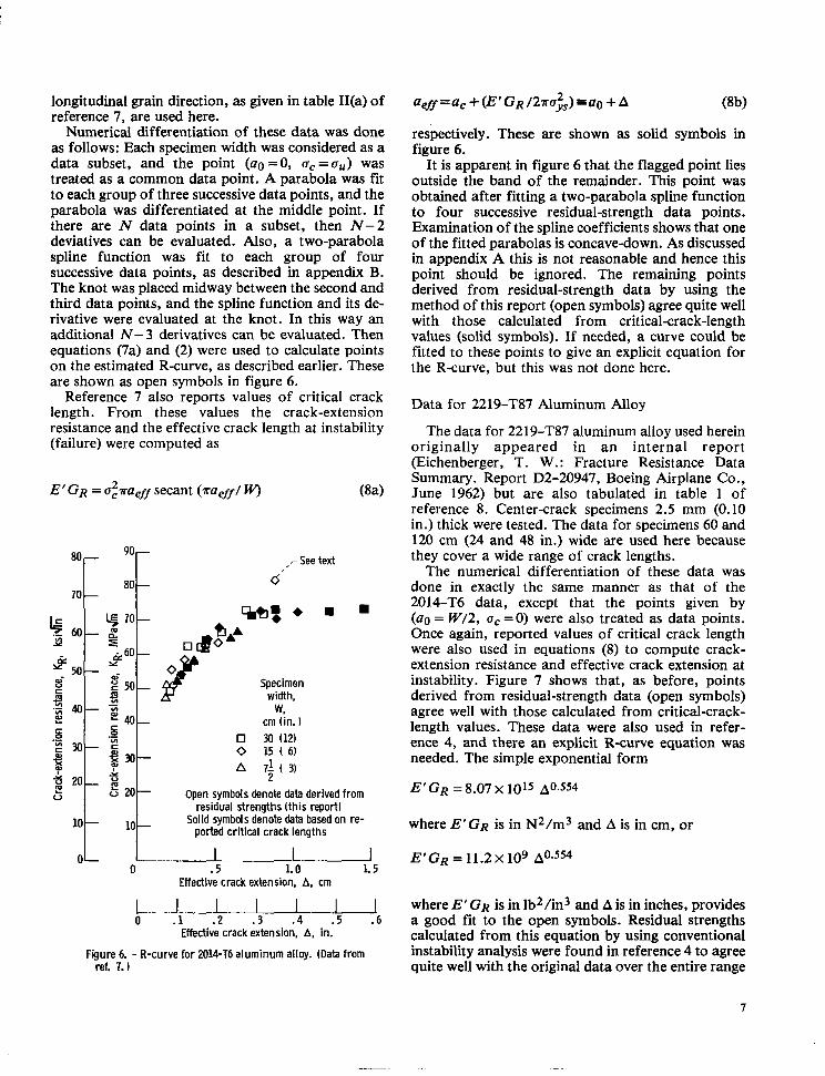
Numerical differentiation of these data was done as follows: Each specimen width was considered as a data subset, and the point (a0 =0, uc =uu) was treated as a common data point. A parabola was fit to each group of three successive data points, and the parabola was differentiated at the middle point. If there are N data points in a subset, then N - 2 deviatives can be evaluated. Also, a two-parabola spline function was fit to each group of four successive data points, as described in appendix B. The knot was placed midway between the second and third data points, and the spline function and its de- rivative were evaluated at the knot. In this way an additional N - 3 derivatives can be evaluated. Then equations (7a) and (2) were used to calculate points on the estimated R-curve, as described earlier. These are shown as open symbols in figure 6.

Reference 7 also reports values of critical crack length. From these values the crack-extension resistance and the effective crack length at instability (failure) were computed as

.-

Y V E 20 'i .- !.I u 20

,-See text

6'

Specimen width.

W. cm (in. 1

0 30 (12) 0 15 ( 6 ) A 7i ( 3)

2 Open symbols denote data derived from

residual strenaths (this reDortl Solid symbols denote data based on re-

ported critical crack lengths

0 .5 1.0 1.5 Effective crack extension, A, cm

I" I I 0 .1 . 2 . 3 . 4 . 5 .6

Effective crack extension, A, in.

Figure 6. - R-curve for 2014-T6 aluminum alloy. (Data from ref. 7.)

aeff = a, + (E' GR /27ru&) a0 -t A (8b)

respectively. These are shown as solid symbols in figure 6.

It is apparent in figure 6 that the flagged point lies outside the band of the remainder. This point was obtained after fitting a two-parabola spline function to four successive residual-strength data points. Examination of the spline coefficients shows that one of the fitted parabolas is concave-down. As discussed in appendix A this is not reasonable and hence this point should be ignored. The remaining points derived from residual-strength data by using the method of this report (open symbols) agree quite well with those calculated from critical-crack-length values (solid symbols). If needed, a curve could be fitted to these points to give an explicit equation for the R-curve, but this was not done here.

Data for 2219-T87 Aluminum Alloy

The data for 2219-T87 aluminum alloy used herein originally appeared in an internal report (Eichenberger, T. W.: Fracture Resistance Data Summary. Report D2-20947, Boeing Airplane Co., June 1962) but are also tabulated in table 1 of reference 8. Center-crack specimens 2.5 mm (0.10 in.) thick were tested. The data for specimens 60 and 120 cm (24 and 48 in.) wide are used here because they cover a wide range of crack lengths.

The numerical differentiation of these data was done in exactly the same manner as that of the 2014-T6 data, except that the points given by (a0 = W/2, uc =0) were also treated as data points. Once again, reported values of critical crack length were also used in equations (8) to compute crack- extension resistance and effective crack extension at instability. Figure 7 shows that, as before, points derived from residual-strength data (open symbols) agree well with those calculated from critical-crack- length values. These data were also used in refer- ence 4, and there an explicit R-curve equation was needed. The simple exponential form

E'GR = 8.07 X 1015 Ao.554

where E'GR is in N2/m3 and A is in cm, or

E'GR = 11.2 x lo9 A0.554

where E'GR is in lb2/in3 and A is in inches, provides a good fit to the open symbols. Residual strengths calculated from this equation by using conventional instability analysis were found in reference 4 to agree quite well with the original data over the entire range

7

Fitted exponential curve (see text)-,

5 .- Y v) 120t

2ok

Specimen width,

W, cm (in. J

0 120 (48) 0 60 (24)

Open symbols denote data derived from

Solid symbols denote data based on re- residual strengths (this report)

ported critical crack lengths

OL , 0 2 4 6 8 10 12

Effective crack extension, A, cm

1 0 1 2 3 4 5

Effective crack extension, A, in.

Figure 7. - R-curve for 2219-T87 aluminum alloy. (Data from ref. 8.)

of crack lengths, with the average error being less than 3 percent.

Data for AM355 Alloy Steel Sheet

Reference 9 includes some unusual test data for AM355 alloy steel specimens 0.5 mm (0.02 in.) thick. One series of tests used specimens of various sizes having a constant ratio of initial crack length to specimen width (Case 11). Another series was run with constant initial crack length and varying widths (Case 111). In addition, a considerable amount of subcritical crack growth data is reported.

Specimens with and without stiffeners (to prevent local crack buckling) were tested, but only stiffened- specimen data are considered here. Numerical differentiation of the constant-ratio (Case 11) data (table XI, ref. 9) was done in the same manner as before except that the point (ac =uu, a0 =0) was not used. Then equations (7b) and (2) were used to calculate points on the estimated R-curve. The constant-crack-length (Case 111) data required a different treatment. The residual-strength data (table VI, ref. 9) are plotted in figure 8. One point appears to be erroneously low and was ignored. The re- maining points do not lie along a simple, smooth curve, and direct numerical differentiation would not

0 J 0 10 20 x) 40 50 60

Specimen width, W, cm ~~ ..

1 0 4 8 12 16 20 24

Specimen width, W, in.

Figure 8. - Residual strength and fitted curve for AM355 steel. (Data from ref. 9. ) Initial crack length, 2a 10 cm(4 in. ); ultimate tensile strength, ou, 1660MPa (2g.8 ksi).

'@'I- I 0

t 4

0 200 (.

I Basis

0

d o b

for calculation

0 Residual strength, ho = Constant

V m L 0 Residual strength, 2a0 =

0 1 2 3 4 5 Effective crack extension, A, cm

u 0 . 4 .8 L 2 16

Effective crack extension, A, in.

Figure 9. - R-curve for AM355 steel. (Data from ref. 9 . )

8

be prudent. Some type of data smoothing is needed. The equation plotted in figure 8 is relatively simple, has the proper curvature and limits, and appears to fit the data fairly well. This equation was used to compute smoothed values of stress (which replaced the experimental values) and associated derivatives. These were then used in equations (7c) and (2) to calculate points on the estimated R-curve. Subcritical crack growth data are presented in figures 20 and 22 of reference 9. These consist of four to eight points per specimen and were taken during the constant- ratio (Case 11) tests. For each point the crack- extension resistance and the effective crack length were calculated by using equations (8).

Points on the estimated Rcurve, computed by three methods, are shown in figure 9 and are in generally good agreement. Those derived from the constant-crack-length (Case 111) residual-strength tests lie along the high side of the scatter band, and this may be due to the choice of the function used to smooth the data.

Concluding Remarks This report has presented a method for estimating

the R-curve from residual-strength data. The method

was verified by using various types of residual- strength data from the literature. Numerical differentiation of the residual-strength data is required, and the data used herein presented no significant problems in that respect.

For other data not examined here the success or failure of the method hinges on the numerical differentiation process, which for residual-strength data is not a well-established procedure. Some guidelines are given in appendix A, but engineering judgment may still be required. If the data can be differentiated with confidence, the method should be successful. If not, the results can be misleading or erroneous. In that case it may be better to fit the data to a semiempirical fracture analysis and derive an equivalent R-curve by using the method of refer- ence 4.

Lewis Research Center, National Aeronautics and Space Administration,

Cleveland, Ohio, May 20, 1980, 505-33.

9

Appendix A

Numerical Differentiation of Residual-Strength Data

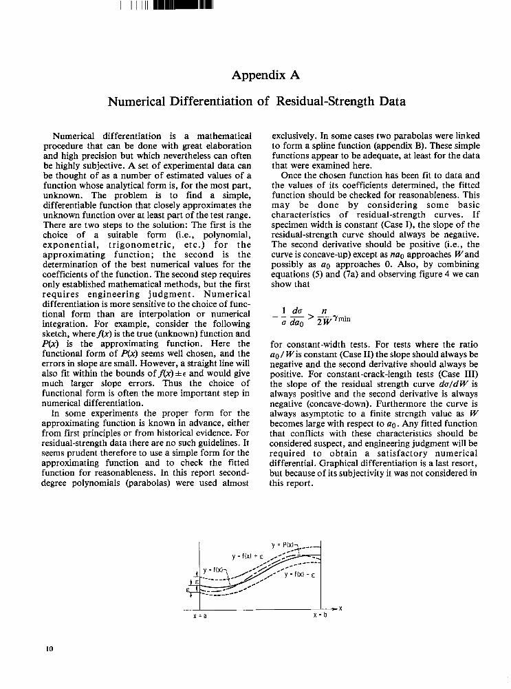
Numerical differentiation is a mathematical procedure that can be done with great elaboration and high precision but which nevertheless can often be highly subjective. A set of experimental data can be thought of as a number of estimated values of a function whose analytical form is, for the most part, unknown. The problem is to find a simple, differentiable function that closely approximates the unknown function over at least part of the test range. There are two steps to the solution: The first is the choice of a suitable form (i.e., polynomial, exponential , tr igonometric, etc.) for the approximating function; the second is the determination of the best numerical values for the coefficients of the function. The second step requires only established mathematical methods, but the first requires engineering judgment. Numerical differentiation is more sensitive to the choice of func- tional form than are interpolation or numerical integration. For example, consider the following sketch, whereflx) is the true (unknown) function and P(x) is the approximating function. Here the functional form of P(x) seems well chosen, and the errors in slope are small. However, a straight line will also fit within the bounds of f (x) and would give much larger slope errors. Thus the choice of functional form is often the more important step in numerical differentiation.

In some experiments the proper form for the approximating function is known in advance, either from first principles or from historical evidence. For residual-strength data there are no such guidelines. It seems prudent therefore to use a simple form for the approximating function and to check the fitted function for reasonableness. In this report second- degree polynomials (parabolas) were used almost

exclusively. In some cases two parabolas were linked to form a spline function (appendix B). These simple functions appear to be adequate, at least for the data that were examined here.

Once the chosen function has been fit to data and the values of its coefficients determined, the fitted function should be checked for reasonableness. This may be done by considering some basic characteristics of residual-strength curves. If specimen width is constant (Case I), the slope of the residual-strength curve should always be negative. The second derivative should be positive (i.e., the curve is concave-up) except as nag approaches Wand possibly as a0 approaches 0. Also, by combining equations ( 5 ) and (7a) and observing figure 4 we can show that

1 da n a dao 2 W

- " - > "Yrnin

for constant-width tests. For tests where the ratio a0 / W is constant (Case 11) the slope should always be negative and the second derivative should always be positive. For constant-crack-length tests (Case 111) the slope of the residual strength curve da/dW is always positive and the second derivative is always negative (concave-down). Furthermore the curve is always asymptotic to a finite strength value as W becomes large with respect to ao. Any fitted function that conflicts with these characteristics should be considered suspect, and engineering judgment will be required to obtain a satisfactory numerical differential. Graphical differentiation is a last resort, but because of its subjectivity it was not considered in this report.

y = f ( X ) - E

10

Appendix B

Two-Parabola Spline Function

A spline function is a sequence of piecewise polynomials of degree N > 1 whose coefficients are such that the function itself and its first N - 1 deriva- tives are continuous over its entire range. The junctions of the polynomials are called knots. In this report some of the numerical differentiation was accomplished by fitting two parabolas through four consecutive data points to form a spline function. The function and its first derivative were then evaluated at the knot, which was midway between the second and third points. This is done as follows.

Let four consecutive data points be denoted as (xi, ui) where x1 <x2 <x3 <x4. We wish to fit two parabolas through the four points such that

If the knot is located at x=xk such that x2 <x& e x 3 , the continuity conditions at the knot are

where the prime denotes differentiation. After subtracting the appropriate part of equation (B2)

from each of equations (Bl), expanding and rearranging terms, and substituting equation (B3), equations (Bl) can be written as

which are easily solved. When differentiating residual-strength data, this approach has two advantages. First, the interpolation value y k and the derivative y i are obtained directly. Second, the signs of the coefficients a 2 and P2 indicate the curvature of the parabolas. As discussed in appendix A, both a 2 and 0 2 should be positive for Case I or Case I1 data and negative for Case I11 data. If a 2 and P2 have opposite signs, there will be an inflection at the knot and the derivative should be regarded with suspicion. If the remaining coefficients are desired, they are

11

References

1. Heyer, R. H.: Crack Growth Resistance Curves (R-Curves)-Literature Review. Fracture Toughness Evaluation by R-Curve Methods. Am. SOC. Test. Mater. Spec. Tech. Publ. 527, 1973, pp. 3-16.

2. Liu, A. F.; and Creager, M.: On the Slow Stable Crack Growth Behavior of Thin Aluminum Sheet. Mechanical Behavior of Materials, Vol. I: Deformation and Fracture of Metals. Society of Materials Science (Japan), 1972, pp. 558-568.

3. Tentative Recommended Practice for R-Curve Determination. Standard E561-78T, Pt. 10, American Society for Testing and Materials, 1979, pp. 616-635.

4. Orange, Thomas W.: A Relation Between Semiempirical Fracture Analyses and R-Curves. NASA TP-1600, 1980.

5 . Brown, W. F.; and Srawley, J . E.: Plane Strain Crack Toughness Testing of High Strength Metallic Materials. Am.

SOC. Test. Mater. Spec. Tech. Publ. 410, 1966, Discussion by C. E. Feddersen, pp, 77-79.

6. Srawley, J. E.: Wide Range Stress Intensity Factor Expressions for ASTM E 399 Standard Fracture Toughness Specimens. Int. J. Fract., vol. 12, no. 3, June 1976, pp. 475-476.

7. Orange, Thomas W.: Fracture Toughness of Wide 2014-T6 Aluminum Sheet at -320" F. NASA TN D-4017, 1967.

8. Kuhn, P.: Strength Calculations for Sheet-Metal Parts with Cracks. Mater. Res. Stand., vol. 8, no. 9, Sept. 1968, pp.

9. Forman, R. G . : Experimental Program to Determine Effect of Crack Buckling and Specimen Dimensions on Fracture Toughness of Thin Sheet Materials. AFFDL-TR-65-146, Air Force Systems Command, 1966 (AD-483308).

21-26.

12