meteorology for seafarers
TRANSCRIPT


METEOROLOGY FOR SEAFARERS ORIGINALLY
METEOROLOGY FOR SEAMEN
BY
COMMANDER C. R. BURGESS, R.N., F.R.Met.S.
REWRITTEN AND COMPLETELY REVISED BY
LIEUTENANT-COMMANDER R. M. FRAMPTON, R.N., F.N.I., F.R.Met.S., F.R.S.A.
AND
P. A. UTTRIDGE, B.Sc, M.Sc„ F.R.Met.S.
GLASGOW
BROWN, SON & FERGUSON LTD., NAUTICAL PUBLISHERS
4-10 DARNLEY STREET

Copyright in all countries signatory to the Berne Convention
All rights reserved
First Edition 1988
Second Edition 1997
ISBN 0 85174 636 5 ISBN 0 85174 530 X (First Edition)
© 1997 BROWN, SON & FERGUSON LTD., 4 - I O D A R N L E Y S T R E E T , G L A S G O W G41 2SD
PREFACE
Commander C. R. Burgess, former Meteorological Officer in the UK Meteorological Office, Bracknell and in the Royal Navy, completed Meteorology For Seamen in 1950 soon after he joined the Marine Society as Secretary. His book has been a standard work for 30 years, combining the factual presentation of the subject with the then popular question and answer format. A further revision became necessary soon after his death in 1982, and the present authors with some trepidation accepted the task.
So many advances have been made in this science and the presentation of text books so changed, that it was decided to present a completely rewritten and revised text with new illustrations. The question and answer format has been abandoned as it is out of place in a book which aims to present the fundamentals of the subject and highlight those aspects of particular interest to all seafarers. It does not aim to provide a simple explanation, as this is regularly and professionally done by the radio, television and the more elementary textbooks, nor does it delve into the highly complex explanations provided by research papers. The interaction of the seas and the atmosphere is considered, but no attempt has been made to treat this important subject fully, since there are many excellent works to which the seafarer should refer to improve his understanding.
Meteorology for Seafarers is therefore a technical book which aims to explain the complexities of the atmosphere and provide the information needed for professional seafarers aspiring to first class certificates of competency. If at the same time it encourages the seafaring reader to investigate and understand more clearly the forces of nature which affect his daily life, then it will have achieved the full ambitions of its authors.
PREFACE TO THE SECOND EDITION
The opportunity has been taken in this Second Edition to update where necessary the text and illustrations. In particular Greenwich Mean Time has been replaced by Universal Time Zone, and Forecast areas and forecasts (Figs 11.1-11.4 and Table 11.4) have been modified.
iii

ACKNOWLEDGEMENTS
The authors and publishers are indebted to and have great pleasure in acknowledging the help, guidance and hard work of so many in the preparation of this book and in particular Captain G. V. Mackie, Captain J. F. T. Houghton, Mr G. Allen and Captain S. Norwell, The Marine Division, UK Meteorological Office; Mr. P. E. Baylis, University of Dundee; Captain E. H. Beetham; Mr P. Bascombe; Mr N. Brown; Mr J. Connaughton, World Meteorological Organization; Captain R. A. Cooper RFA; Captain J. C. Cox; Mr I. W. Cullen; Mr W. G. Davison; Mr W. T. L. Farwell; Mr N. D. Ferguson; Mr J. R. Gilburt; Dr F. A. James; Mrs E. Koo, Royal Hong Kong Observatory; Mr C. R. Little, London Weather Centre; Mr L. McDermid; Captain D. M. McPhail; Captain J. McWhan; Captain S. D. Mayl; Mr C. D. Mercer; Captain S. R. Montague; Mr M. Moore; Mr J. W. Nickerson; Mr R. K. Pilsbury; Mr D. G. Robbie; Captain P. Thompson; Mr I. Thomson, Mr R. F. Williams; David Henderson for the diagrams; and the staff of The Marine Society, particularly Miss D. Durrant and Miss F. Musa who typed the script.
The following copyrights and sources are acknowledged with thanks: Her Majesty's Stationery Office (HMSO) (Crown Copyright; UK Meteorological Office and The Hydrographer of the Navy): Figs. 2.1,6.5,7.9,8.1,8.3,8.4,8.6,8.10,8.14,8.16,9.3,9.12,9.13,9.15,9.16,10.2,10.4,10.9-10.12,10.14-10.18,10.20, 11.1-11.4, 11.6-11.8,Tables7.1,7.2,andTables 11.3, 11.4. World Meteorological Organization: Figs. 10.3,10.6,10.7, Tables 6.1, 6.2, Appendix 2-2.1,2.2. Negretti Aviation: Fig. 2.2. US Mariners Weather Log and US Department of Commerce, National Oceanic and Atmospheric Administration: Fig. 2.6, Appendix 1, Table A.l. Seaways: Appendix 1. R. G. Barry and R. J. Chorley, Atmosphere, Weather and Climate (Methuen): Fig. 4.5. Casella London Ltd: Fig. 4.7. Mr M. J. Leeson: Fig. 6.3. Australian Bureau of Meteorology, Melbourne: Figs. 8.11 and 10.13. The Royal Observatory, Hong Kong: Figs. 9.1 and 9.2. The European Space Agency: Figs. 9.5(1), 9.5(2), 10.5(3) and 10.5(4). D. Riley and L. Spolton, World Weather and Climate (Cambridge University Press): Figs. 9.7, 9.17 and 9.18. J. G. Lockwood, World Climatology—An Environmental Approach (E. Arnold): Fig. 9.14. Mr S. Whitelock: Fig. 10.4. University of Dundee: Figs. 10.5(1) and 10.5(2). Furuno(UK)Ltd:Fig. 11.5.
Colour Plates The authors received a very great number of colour photographs of cloud, sea states and
meteorological phenomena, and are most grateful to the following contributors for their permission to use their work (Plate No): Captain S. J. Allen—12, 13, 14; Captain E. H. Beetham—21, 22, 23, 33, 34, 35; Mr P. Bascombe—39; Mr N. Brown—27, 42; Mr C Doris—24; Mr J. R. Gilburt—19, 26, 36,41, 43; Captain S. D. Mayl—25, 30; Mr M. Moore—10; Mr R. K. Pilsbury—2-2, 6; Captain C. R. Reed—16; Mr D. G. Robbie—1, 2-1, 11,15, 31, 37, 38, 40; Captain J. F. Thomson—44; Front Cover: Peter Knox—Storm Petrel.
v

CONTENTS
PREFACE
ACKNOWLEDGEMENTS
LIST OF ILLUSTRATIONS AND PLATES
LIST OF TABLES
CHAPTER 1 THE ATMOSPHERE Introduction Structure and Composition Density and Pressure Temperature
CHAPTER 2 ATMOSPHERIC PRESSURE Introduction Definition Barometers Isobars Pressure Tendency Barographs Diurnal Variation and Range
CHAPTER 3 TEMPERATURE Introduction Observation Solar and Terrestrial Radiation Energy Transfer Diurnal Variation and Range Environmental Lapse Rate
CHAPTER 4 WATER IN THE ATMOSPHERE States of Water Water Vapour Relative Humidity Dew-point Temperature Condensation Evaporation Diurnal Variation of Relative Humidity Hygrometers
CHAPTER 5 CLOUDS Introduction Cloud Types Adiabatic Lapse Rate
v

VIII CONTENTS
Atmospheric Stability Formation of Clouds
CHAPTER 6 PRECIPITATION AND FOG Forms of Precipitation Development Observation Visibility Fog Haze
CHAPTER 7 WIND Definition Observation Large Scale Air Flows Sea and Land Breezes Katabatic and Anabatic Winds
Page 29 29
32 32 35 35 36 38
39 39 42 47 48
CHAPTER 8 TEMPERATE AND POLAR ZONE CIRCULATION General Circulation of the Atmosphere Frontal Depressions Troughs of Low Pressure Secondary Depressions Anticyclones Ridges of High Pressure Cols Air Masses
CHAPTER 9 TROPICAL AND SUBTROPICAL CIRCULATION Introduction Tropical Cyclones Intertropical Convergence Zone Equatorial Trough Doldrums Trade Winds Monsoons Monsoon Type Weather
CHAPTER 10
CHAPTER 11
ORGANIZATION AND OPERATION OF METEOROLOGICAL SERVICES
Introduction The World Meteorological Organization Land Observing Network Sea Observing Network Meteorological Data Transmission Satellites Global Telecommunications System Data Analysis Forecasting Techniques Ship Routeing Services
FORECASTING SOURCES Single Observer Forecasting Issued Meteorological Data
49 51 61 63 63 65 65 66
70 71 81 83 83 85 85
89 89 89 90 93 94 98 98 103 105
109 110

CONTENTS IX
Page Requested Meteorological Data 117 Facsimile Charts 118 Utilization of Facsimile Data 120 Climatic Data 123
APPENDIX 1—Typhoon Faye and Extreme Storm Waves 125
APPENDIX 2—World Meteorological Organization—Areas of responsibility for the issue of weather and sea bulletins 128
APPENDIX 3—Other sources of information 130
INDEX 132

ILLUSTRATIONS AND PLATES
Chapter Figure Title Page
1 THE ATMOSPHERE 1.1 Air temperature distribution for the standard atmosphere 1 1.2 Density and pressure distribution for the standard atmosphere 2
2 ATMOSPHERIC PRESSURE 2.1 Simple Aneroid Barometer 3 2.2 Precision Aneroid Barometer 5 2.3 Isobars 6 2.4 Marine Barograph 7 2.5 Barograms 8 2.6 Barogram—tropical cyclone (Typhoon Faye) 9
3 TEMPERATURE 3.1 Marine Screen 11 3.2 Solar and terrestrial radiation 12 3.3 The Radiation Budget 13 3.4 Diurnal variation and range of temperatures 15 3.5 Environmental Lapse Rates 17
4 WATER IN THE ATMOSPHERE 4.1 States of water 19 4.2 The Saturation Curve 20 4.3 Frost Point 21 4.4 Mixing of air samples 22 4.5 Average annual evaporation distribution for ocean areas 23 4.6 Diurnal variation of relative humidity 23 4.7 Whirling Psychrometer 24
5 CLOUDS 5.1 Condensation of water vapour 27 5.2 Atmospheric stability 28 5.3 Formation of clouds 30
6 PRECIPITATION AND FOG 6.1 Development of precipitation 32 6.2 Ice crystal development 33 6.3 Hailstone 34 6.4 Development of hailstones 34 6.5 Distribution of sea fog 37 6.6 Forecasting sea fog 37
7 WIND 7.1 Wind vane and anemometer 39
XI

xii ILLUSTRATIONS AND PLATES
Figure
7.2 7.3 7.4 7.5 7.6 7.7 7.8 7.9 7.10 7.11 7.12 7.13
Title
True wind vector triangle Horizontal pressure gradient Pressure gradient force and air flow Geostrophic wind Gradient wind Angle of indraught Buys Ballot's Law Surface wind Sea breeze Land breeze Katabatic wind Anabatic wind
Page
42 42 43 43 44 45 45 46 47 47 48 48
8.1 8.2 8.3 8.4 8.5 8.6 8.7 8.8 8.9 8.10 8.11 8.12 8.13 8.14 8.15 8.16
TEMPERATE AND POLAR ZONE CIRCULATION General circulation of the atmosphere—idealized Frontal zone—vertical section Temperate and polar zone circulation—surface synoptic chart Mean position of frontal zones Life cycle of a polar front depression-surface plan view Surface synoptic charts Polar front jet stream and a frontal depression Plan and elevation of a typical frontal depression in the N Hemisphere Warm and cold occlusions Local winds of the Mediterranean Typical surface synoptic chart for the S Hemisphere Plan of a frontal depression in the S Hemisphere Troughs of low pressure Secondary depressions Characteristics of an anticyclone Air masses—typical surface synoptic charts
49 50 50 51 52
53-54 55 56 57 59 60 60 61 62 64
67-69
9.1 9.2 9.3 9.4 9.5 9.6 9.7 9.8 9.9 9.10 9.11 9.12 9.13 9.14 9.15 9.16 9.17 9.18
TROPICAL AND SUBTROPICAL CIRCULATION Tropical and subtropical circulation—typical surface synoptic chart Tropical storm—typical surface synoptic chart Distribution and tracks of tropical cyclones Tropical cyclone—elevation Tropical cyclone—geostationary satellite images Tropical cyclone—surface plan view Tropical cyclones—N Atlantic Tropical cyclone—wind and pressure distribution Evasive action—N Hemisphere Evasive action—S Hemisphere Streamline chart for the N Pacific Intertropical Convergence Zone Equatorial Trough The Doldrums Tropical and subtropical zones—January Tropical and subtropical zones—July North-East Monsoon—typical surface synoptic chart for a day South-West Monsoon—typical surface synoptic chart for a day
n January in July
70 71 72 73 74 75 76 78 80 81 82 82 83 83 84 84 86 86

ILLUSTRATIONS AND PLATES XIII
Chapter Figure
10
10.1 10.2 10.3 10.4 10.5 10.6 10.7 10.8 10.9 10.10 10.11 10.12 10.13 10.14 10.15 10.16 10.17 10.18 10.19 10.20
11 11.1 11.2 11.3 11.4 11.5 11.6 11.7 11.8
APPENDIX 2
2.1 2.2
Title
ORGANIZATION AND OPERATION OF METEOROLOGICAL SERVICES Observing network Ocean Weather Ship stations Ship and land station code format Data Buoy Satellite images Geostationary satellite Polar orbiting satellite Global Telecommunications System Coded observations plotted in station model format Computer plot of surface reports Surface synoptic chart Completed surface synoptic chart Circumpolar surface synoptic chart 500 hPa contour chart 1000-500 hPa thickness chart Computer output of isobars for a surface prognostic chart Wave prognostic chart Typical vessel performance curves Least-time technique Voyage analysis
FORECASTING SOURCES Atlantic Weather Bulletin—Forecast areas High Seas Weather Bulletin—Forecast areas Shipping forecast areas Typical Port Meteorological Office forecast Facsimile equipment Surface synoptic chart Surface prognostic charts (24,48 and 72 hours) Sea ice chart
WORLD METEOROLOGICAL ORGANIZATION-WEATHER AND SEA BULLETINS World South-West Pacific Region
Page
90 90 93 94
95-96 97 97 98 99 99
100 100 101 102 102 104 105 106 107 108
114 115 116 117 118 119
120-121 222
128 129
PLATES 1-16 Clouds and other meteorological phenomena

COLOUR PLATES
A CLOUDS AND METEOROLOGICAL PHENOMENA
Plate No.
1. 2.1 2.2 3 4 5 6 7 8 9
10 11 12) 1 3
14 15 16 17 18 19 20 21] 22 23 24 25 26 27 28 29-ll 29-2
Title
Cirrus (Ci) Cirrostratus (Cs) Cirrostratus (Cs) with halo Cirrocumulus (Cc) Altostratus (As) Altocumulus (Ac) Stratus (St) Stratocumulus (Sc) Nimbostratus (Ns) Cumulus (Cu) Cumulus (Cu) Cumulonimbus (Cb) Cumulonimbus—developing from cumulus (12), after ten minutes (13) and after forty minutes (14) Cumulus (Cu) and Stratocumulus (Sc) Waterspout Orographic cloud Lenticular cloud Cumulonimbus precipitating Lightning Entering seafog in the English Channel
Arctic Sea Smoke—St Lawrence Seaway Pampero Effect of a temperature inversion—North Sea Trade wind cumulus Rainbows—primary and secondary
Contrails
XV

XVI COLOUR PLATES
B SEA STATES AND STORM WAVES
Plate No.
30 31 32 33 34 35 36 37 38 39 40 41 42 43 44
Title
Force 0 Force 1 Force 2 Force 3 Force 4 Force 5 Force 6 Force 7 Force 8 Force 9 Force 10 Force 11 Force 12 Swell and wind waves Force 2-3 Extreme storm wave, North Atlantic, Force 12

LIST OF TABLES
Chapter Table Title Page
5 CLOUDS 5.1 Cloud genera 26 5.2 Description of cloud genera 27
6 PRECIPITATION AND FOG 6.1 Visibility scale used on land 35 6.2 Visibility scale used at sea 35
7 WIND 7.1 The Beaufort Scale 40 7.2 Swell waves 41
8 TEMPERATE AND POLAR ZONE CIRCULATION 8.1 Weather sequence of a frontal depression to the south of the observer in
the N Hemisphere 58 8.2 Weather sequence of a frontal depression to the north of the observer in
the N Hemisphere 58 8.3 Weather sequence of cold and warm occlusions in the N Hemisphere 59 8.4 Characteristics of air masses 66
9 TROPICAL AND SUBTROPICAL CIRCULATION 9.1 Tropical cyclone occurrence 72 9.2 Tropical cyclones—terminology 75 9.3 Evasive action by vessel in N Hemisphere 80 9.4 Evasive action by vessel in S Hemisphere 80
10 ORGANIZATION AND OPERATION OF METEOROLOGICAL SERVICES
10.1 Observations recorded by Voluntary Observing Ships 91 10.2 Statistics relating to Voluntary Observing Ships—International 92 10.3 Voluntary Observing Ships—UK Meteorological Office Register 92
11 FORECASTING TECHNIQUES 11.1 Onboard observations 109 11.2 Publications listing radio weather services 110 11.3 Structure of a weather bulletin 111 11.4 Weather Bulletins 112-113 11.5 Requested meteorological data available from the United Kingdom 117 11.6 Routeing chart data 123
APPENDIX 1 TYPHOON FAYE AND EXTREME STORM WAVES
A-l Classification of Extreme Storm Waves 127
B

CHAPTER 1
THE ATMOSPHERE
INTRODUCTION
Meteorology is the scientific study of the atmosphere. The atmosphere is the envelope of gases surrounding the earth in which a number of processes varying in duration and dimension operate. These result in the weather experienced by an observer on the surface of the earth. Climate is the more general pattern of weather established by analysing, on an annual basis, the daily conditions at a particular point.
STRUCTURE AND COMPOSITION
The atmosphere may be considered as having a number of distinctive layers which are defined by the variation of air temperature with increase in height. For the standard atmosphere (Fig. 1.1) the layers are:
(a) Troposphere—Surface of the earth to 12 km—the tropopause. (b) Stratosphere—Tropopause to 47 km—the stratopause. (c) Mesosphere—Stratopause to 80 km—the mesopause.
Above the mesopause lies the thermosphere, a layer with a negligible quantity of gas, whose temperature increases with increase in height. It should also be noted that other layers may be defined on different criteria. The ionosphere for example, where the gases ionized by solar radiation affect the propagation of radio waves, exists from 60 km upwards.
Below the mesopause the mixture of gases in the atmosphere is nearly constant:
Gas Nitrogen (N2) Oxygen (02) Argon (Ar) Carbon dioxide (C02)
Percentage By Volume 78.09 20.95
0.93 0.03
MESOPAUSE
STRATOPAUSE
-40 -20 0 20
TEMPERATURE <°C)
Fig. 1.1 Air temperature distribution for the standard atmosphere.
1

2 METEOROLOGY FOR SEAFARERS
There are also traces of neon, helium, krypton, hydrogen and xenon. Ozone occurs at a greater level of concentration in the stratosphere, and this layer may be termed the ozonosphere.
In the troposphere, other chemical compounds are also present of which water vapour is by far the most significant. The amount of water vapour varies both in space and time, being greater in the lower troposphere and decreasing with increasing height. The volume of water vapour may be as much as 4% which, although small compared with the total volume of the atmosphere, is very significant in terms of the amount of energy which the atmosphere is able to store (Chapters 3 and 4). Other substances which may also be present are particles from the surface of the earth and from outer space, and chemical compounds which are manufactured within the atmosphere from the constituents present. Dramatic and sometimes unpleasant and damaging effects can be produced by these various substances; for example colourful sunsets and sunrises, red and acid rains.
Density and Pressure
The density of the gases decreases with increasing height (Fig. 1.2) since they are compressible, and 75% of the total mass of air is within the troposphere.
At the surface the standard atmospheric pressure is 1013.2 hPa (hectopascal) (Fig. 1.2), the equivalent of a tonne load on a man's shoulder. With increasing height atmospheric pressure decreases. This trend is partly related to the decrease of air density with increase in height. It should be noted that, while the value of the pressure at the surface in Fig. 1.2 relates to the standard atmosphere, actual values observed vary significantly from the standard (Chapter 2).
Temperature
in tne tropospnere air temperature normally decreases as neignt increases. The slope of the line in Fig. 1.1 illustrates this change or lapse rate. As the slope relates to air temperature, it is termed the Environmental Lapse Rate (E.L.R.). For the standard atmosphere, where the air temperature at the surface is 15°C, the E.L.R. value in the troposphere is 6.5°Ckm_1. The tropopause, the boundary of the troposphere with the stratosphere, is defined as the level at which the rate of decrease of temperature is 2°Ckm~1 or less, provided that the average decrease of temperature within the next 2 km does not exceed 2°C km " 1 . In the standard atmosphere the tropopause is located at 12 km. However, in the actual atmosphere its height varies from 16 km at the equator to 9 km at the poles.
In the lower stratosphere, air temperature is constant with increasing height, but in the middle and upper parts it increases with increasing height. This temperature profile reflects the presence of ozone. In the mesosphere air temperature decreases rapidly with increasing height to — 80°C at the mesopause.

CHAPTER 2
ATMOSPHERIC PRESSURE
INTRODUCTION
Atmospheric pressure is the most important meteorological element observed since it is the principal guide to the state of the atmosphere at a given time. The weather map or surface synoptic chart is derived from a set of readings of this element taken at different locations at internationally agreed times known as synoptic hours. The principal synoptic hours are 0000, 0600, 1200 and 1800 UTC.
DEFINITION
Pressure may be defined as the force which is exerted on unit area of a surface. The term atmospheric pressure therefore refers to the force which a column of air exerts on unit area of the earth's surface. The formula which defines this pressure is P = pgh where P is the pressure, p the mean density of the air in the column, g the value of gravity, and h the height of the air column. The unit of measurement of atmospheric pressure is the hectopascal (hPa), this unit being equivalent to and having recently replaced the millibar (mb) (1 hPa = 1 mb = 102 Nm"2, where N is a newton which is equal to 1 kg m1 s"2).
At any height above the surface of the earth the atmospheric pressure will be less than that at the surface. This is due to the smaller values of both the height of the air column and the mean density of air in the column (Fig. 1.2).
BAROMETERS
For many years the aneroid and mercury barometers have been used to determine atmospheric
Fig. 2.1 Simple Aneroid Barometer.
3

4 METEOROLOGY FOR SEAFARERS
pressure. The precision aneroid barometer is considered to be the most accurate instrument for observing purposes.
Simple Aneroid Barometer
The principle on which all aneroid barometers are based is the use of the elastic properties of a metal to monitor changes in atmospheric pressure, and hence its value at a given time. With the simple aneroid barometer (Fig. 2.1) the metal, in the form of a corrugated capsule (1) almost exhausted of air, is compressed when the atmospheric pressure increases, and expands when the pressure decreases. The capsule is supported by a spring (2), and by means of a linkage system (3) its movement can be magnified. This is shown by a moving pointer (4) which rotates over a dial graduated in hectopascals. The metal from which the instrument is constructed is affected by changes in air temperature, which will result in an inaccurate reading. The effect is compensated for by leaving a small amount of air in the capsule and incorporating a bimetallic linkage (5). The elastic properties of the metal capsule change with time, and the instrument should therefore be checked at frequent intervals against an accurate barometer to determine its index error. This error is removed by means of the screw located in the back of the instrument.
The simple aneroid barometer can be used not only to record the atmospheric pressure to the nearest hectopascal at a given time, but also to observe the change in pressure over a period. By using the knurled knob (6) to set the pointer (7) at the current position of the moving pointer (4), the observer can note the change over the period by comparing the position of the moving pointer with the set pointer.
Precision Aneroid Barometer
The precision aneroid barometer (Fig. 2.2) is the instrument used to obtain readings of atmospheric pressure to the nearest tenth of a hectopascal, which are essential in the production of accurate synoptic charts. The accuracy of the reading is achieved by incorporating three aneroid capsules, and an improved magnification system and method of registering atmospheric pressure. The observer controls the magnification and registering of atmospheric pressure by using the external knob (A) to adjust the position of the micrometer screw (B). The position of the latter determines whether or not it is in contact with the contact arm (C). To obtain a reading the external knob is turned until contact between the micrometer screw and contact arm is made. The contact is indicated by a continuous line of light on the external display (D), when the button (E) is depressed. The external knob is then turned until the line of light just breaks, which indicates that the contact between the micrometer screw and the contact arm is just broken. At this point the readout (F) indicates the atmospheric pressure exerted on the capsules. Compensation for temperature variation of the instrument is provided by the inclusion of a small amount of air in the capsules. A pressure choke can be fitted (at position G) which restricts instrument response to short term changes of atmospheric pressure due to factors such as ship motion. The power supply for the electrical circuit is provided by a battery housed within the instrument, access being through the cover (H).
Corrections to Readings
All barometric readings which are to be used for synoptic purposes must be corrected to standard datum. The correction necessary for readings from the precision aneroid barometer are for height above mean sea level and index error. The height correction, obtained from tables, requires the height above mean sea level of the instrument and air temperature, obtained from the marine screen (Chapter 3), to be known. Inclusion of air temperature takes into account the mean density of the air in the column between the height of the instrument and mean sea level. The manufacturer supplies the index error correction which relates to errors inherent in the instrument. However, it is important that the instrument is checked frequently by comparing its readings with that of another barometer of known accuracy. Readings from a simple aneroid barometer included on a synoptic chart are also corrected for height above mean sea level and index error if applicable.


6 METEOROLOGY FOR SEAFARERS
ISOBARS
Corrected atmospheric pressure readings for a synoptic hour are plotted on a chart (Fig. 2.3), where they are compared with each other. Lines can then be drawn on the chart joining points having the same
pressure value, each line being an isobar of a whole hectopascal value, e.g. 996 hPa. The interval between isobars on a chart is always constant, usually being 4 hPa (Fig. 2.3) or 5 hPa. The final isobaric chart thus shows the distribution of surface atmospheric pressure.
PRESSURE TENDENCY
Atmospheric pressure may change over a period, and the change is termed the pressure tendency. For synoptic purposes the interval of time over which the change is observed is the 3 hours preceding the time of observation. The characteristics of the tendency observed may be described as "rising", "falling" or "steady", or a combination of these terms. The amount of change is also noted, being the difference between the reading at the beginning and end of the 3 hour period, to the nearest tenth of a hectopascal. After plotting observed pressure tendencies on a chart, lines termed isallobars are drawn, which join points having the same pressure tendency. The value of an isallobar, either positive or negative, is to the nearest tenth of a hectopascal, and the interval between isallobars is constant. The isallobaric chart thus indicates areas where pressure changes have occurred, and may be used in developing the forecast.

ATMOSPHERIC PRESSURE 7
BAROGRAPHS
The barograph has been designed to record atmospheric pressure and is used to determine the pressure tendency. This instrument works on the aneroid principle, having a number of capsules linked with each other and with a lever system connected to a pen arm. When the capsules respond to changes in atmospheric pressure, the pen arm moves either up or down across a scaled chart attached to a drum rotated by a clockwork mechanism. This record of pressure over a period is termed a barogram.
Fig. 2.4 Marine Barograph.
In the Marine Barograph (Fig. 2.4), the aneroid capsules are enclosed within a brass cylinder containing a silicone fluid. This arrangement acts as a "damping" mechanism, eliminating the response of the instrument to short term changes in pressure due to factors such as ship motion and vibration. However, the instrument is still free to respond to the long term changes of pressure. The clock operates for a period of 7 1/3 days, and the drum is fitted with a 7 day chart which is changed once a week when the clock is wound.
DIURNAL VARIATION AND RANGE
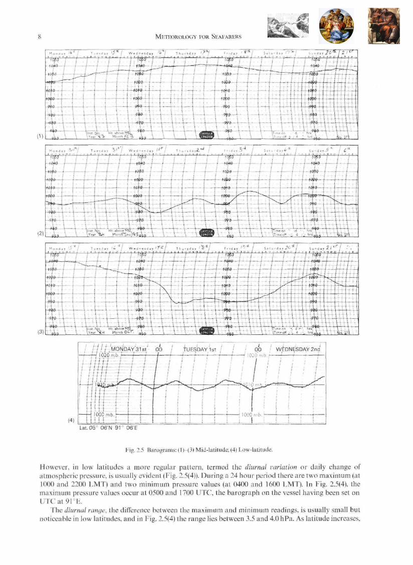
When comparing a number of barograms of mid-latitude observations (Fig. 2.5(1) to (3)), it is particularly noticeable that there is neither a regular pattern nor a mean pressure value evident.

ATMOSPHERIC PRESSURE 9
Fig. 2.6 Barogram tropical cyclone (Typhoon Faye).
the diurnal range observed is smaller, with the result that in mid-latitudes the few tenths of a millibar are masked by the greater changes of pressure associated with pressure systems affecting the area (Fig. 2.5(1) to (3)).
In low latitudes the diurnal variation may be masked by excessive pressure changes due to tropical cyclones (Chapter 9), the decrease in pressure being far greater than the relatively small change attributed to diurnal variation (Fig. 2.6). Pressure tendency is therefore worth recording when in the tropics, for a change may well be the first sign of the approach of a tropical cyclone.

CHAPTER 3
TEMPERATURE
INTRODUCTION
Air temperature may be monitored at various heights above the surface. Surface air temperature is monitored at 1.25 m, the recommended height for instruments on land. Surface temperature is that monitored at the surface, and at land observing stations the surface may be turf, concrete or soil. At sea the surface temperature is monitored by voluntary observing ships or data buoys.
The air temperature recorded can in some circumstances reflect the influence of the underlying surface on a mass of air, and in particular the contrast which exists between land and sea surfaces. On other occasions the air temperature reflects the horizontal movement of air associated with pressure systems (Chapter 8).
OBSERVATION
Air Temperature
The standard instrument for monitoring air temperature is known as the dry-hulh thermometer which is a mercury thermometer enclosed in a glass sheath. The thermometer is housed in a Stevenson Screen which is designed to allow a free flow of air past the instrument, and at the same time eliminates the effects of solar and terrestrial radiation. The temperature is normally recorded to the nearest tenth of a degree Celsius (°C). A platinum resistance thermometer with a digital readout may be used as an alternative to a mercury thermometer.
The screen used at sea is the Marine Screen (Fig. 3.1), which is the Stevenson Screen modified to house the Mason's Hygrometer under seagoing conditions (Chapter 4). The screen is constructed of wood with louvred sides, one of which is a hinged door. The floor is slotted and the roof is a double structure, the inner one having ventilation holes. The entire structure is painted white both internally and externally.
At sea 2 screens are normally used, one being on each bridge wing at a height of about 1.5 m above the deck and sited as far as possible from any of the vessel's heat sources. Observations of air temperature are always obtained from the screen located to windward.
Sea Temperature
Sea surface temperature is generally more difficult to monitor than either land surface or air temperature, and one or more methods may be used depending on the operation of the observing ship. If its deck height and speed permits, a sample of water is collected in a specially designed bucket made of canvas or rubber reinforced by canvas. The bucket is swung clear of the vessel to prevent any contamination of the sample, and submerged to a depth of about 1 m to avoid sea spray, which may be at a different temperature compared with that of the sea surface. Once inboard, the bucket is placed in a suitable position so that any energy transfer which may affect the temperature of the sample is minimized. A mercury thermometer provided with the bucket is used to record the temperature of the sample.
If the above method cannot be used for operational reasons the temperature of the engine room intake is recorded. However, this data is liable to be inaccurate, partly due to the depth of the intake below the surface, and partly through the heating of the water sample as soon as it is inside the vessel.
10

TEMPERATURE 11
Fig. 3.1 Marine Screen.
Distant reading thermometers have been introduced for voluntary observing purposes. An electrical resistance unit is sited on the inside of the hull about 1 m below the waterline, where the hull temperature is similar to that of the sea. The sensing unit is connected to a digital readout located on the bridge, from which the observer can obtain a reading whenever required. This method minimizes the sources of error inherent in the other two techniques, but assumes the draught of the vessel will be more or less constant.
The temperature of the air or surface indicates its internal energy content. The processes involved in the gain or loss of this energy by the surface of the earth and the atmosphere are considered in the following sections.
SOLAR AND TERRESTRIAL RADIATION
The major source of energy driving the atmospheric circulation is the sun. The energy emitted by the sun is radiant energy or radiation in the form of electromagnetic waves, an important characteristic of which are their wavelengths. The sun, with a mean surface temperature of 6000 K, radiates energy within the range of wavelengths of 0.2 to 4 um, with the maximum emission of energy being at the 0.5 um wavelength (1 um = 1 micrometre = 10_6m). Thus solar radiation spans the ultraviolet, visible and infra-red parts of the spectrum.

The surface of the earth, with a mean temperature of 288 K (15°C), radiates energy in the infra-red part of the spectrum within the range of 4 to 100 um wavelength. The maximum emission is at 10 um wavelength. On comparing the wavelengths of radiation of the sun and the surface of the earth the terms shortwave radiation and longwave radiation may be applied respectively (Fig. 3.2).
The atmosphere also radiates energy. For the standard troposphere, within the range of temperatures noted (Fig. 1.2), the radiation emitted will have a similar range of wavelengths to that of the surface and is therefore longwave radiation. Together the radiation from these two sources is termed terrestrial radiation.
Solar Radiation and the Atmosphere
Five major factors affect the amount of solar radiation received at the surface of the earth:
1. Output of energy of the sun. This varies particularly in the amount of ultraviolet radiation which increases during a sunspot maximum.
2. Distance of the earth from the sun. At perihelion (minimum distance) the amount of solar radiation incident upon (i.e. falling onto) a surface at right angles to the solar beam is 7% greater than at aphelion (maximum distance). At its mean distance from the sun, the amount of solar radiation incident at right angles on the outskirts of the atmosphere is 1.396kWm"2. This is termed the solar constant.
3. The altitude of the sun. This depends on the latitude, season and time of day. Generally as the altitude increases the amount of solar radiation incident upon unit area of surface increases.
4. The number of hours of daylight. 5. The transparency of the atmosphere. This together with the above factors dictates the amount of
solar radiation incident upon unit area of the earth's surface in a given period. This amount is termed insolation.
The effect of atmospheric transparency is illustrated in Fig. 3.3 and summarized below, the atmosphere having its normal composition and four eighths cloud cover.
WAVELENGTH {fxm)
Fig. 3.2 Solar and terrestrial radiation.

A. The amount of solar radiation incident on the outer limits of the atmosphere. B. Absorption in the stratosphere, mainly by ozone, of ultraviolet radiation. C. Absorption in the troposphere by gases, water vapour and dust particles. D. Reflection to space by clouds, there being no change in the wavelength of the radiation. E. Scattering of radiation to space.
(Note: Scattering depends mainly on the ratio of the size of the scattering particle to the wavelength of the radiation incident upon it. In the atmosphere the wavelength usually scattered is that of blue light, hence the blue colouring of the sky.)
Amount of solar radiation incident upon the surface of the earth
Units + 100
- 3 - 1 4 - 2 4 - 6
53
Of the 53 units, 6 (F) are reflected by the surface and 47 (G) are absorbed (Fig. 3.3). The solar radiation incident upon the surface may be described as being either diffuse or direct,
indicating whether its passage through the atmosphere has, or has not, been affected by the constituents present.

14 METEOROLOGY FOR SEAFARERS
The total amount of solar radiation reflected to space (D, E and F) is termed the planetary albedo, being the ratio of the solar radiation reflected to that incident on the outer limits of the atmosphere. In this case the planetary albedo is 36%. Its individual components can vary in value. For example if no cloud is present, the 24 units (D) will be incident on the surface, whereas with an extensive cover more than 24 units will be reflected. The albedo value will be influenced by the nature of the surface (forest 5-10%; sand 20-30%; fresh snow 80-90%; sea 7-9%). The angle of incidence of the solar beam upon the surface will also affect the albedo value, which will be of the order of 100% immediately after sunrise and before sunset, and at a minimum when the sun is at the meridian.
In conclusion it should be noted that only 14% (C) of the total amount of incoming solar radiation is directly absorbed by the troposphere. In terms of a gain of energy per unit volume of air the amount is insignificant. In contrast the surface of the earth absorbs a large amount of solar radiation (G).
Terrestrial Radiation and the Atmosphere
While the atmosphere is almost transparent to solar radiation, it is almost opaque to terrestrial radiation absorbing that emitted by the surface and the atmosphere itself. The constituents which play a significant part in the process of absorption are water vapour, carbon dioxide, ozone and cloud, (Fig. 3.3). Assuming the surface has a mean temperature of 288 K (15°C):
Units H. Radiation emitted by the surface. +113 J. The part of H which passes through the atmospheric window to space. — 6 K. The part of H absorbed by the atmosphere. — 107
L. Radiation emitted by the atmosphere which is incident on the surface and absorbed 95
Thus the overall energy loss (H-L) from the surface in the form of longwave radiation is 18 units. On comparing this loss of energy with the gain of 47 units (G), the surface appears to have gained 29
units. However, this energy is transferred to the atmosphere in the form of sensible and latent heat as a result of conduction and evaporation respectively (M). The 58 units of energy which the atmosphere gains through conduction, evaporation and absorption of solar and terrestrial radiation, are eventually radiated to space (N).
The amount of cloud cover and water vapour present will cause variations in energy loss. If the water vapour content is large, or if there is extensive cloud cover at low levels, then a greater part of the longwave radiation emitted by the surface is absorbed by the atmosphere.
In conclusion the atmosphere effectively absorbs terrestrial radiation, but is itself radiating energy continuously. As a large part of the radiant energy emitted by the surface is returned to it, the daily change of air temperature must be attributed to other forms of energy transfer, which are considered below.
ENERGY TRANSFER
The transfer of energy between the surface of the earth and the atmosphere can be attributed to the processes of conduction, convection and evaporation.
Conduction
Conduction is the transfer of energy between two masses which are in contact with each other, from the mass with the higher temperature to that with the lower temperature. The rate at which energy is transferred depends upon the difference of temperature, which is normally expressed in terms of a temperature gradient, and the thermal conductivity of the mass(es). As air is a relatively poor conductor of energy, the process is insignificant within the atmosphere itself. However, where the air is directly in contact with the surface, conduction is important and results in the transfer of energy between atmosphere and surface, depending upon the direction of the temperature gradient.

TEMPERATURE 15
Convection
Convection is the transfer of energy as a result of movement of parts of a fluid. Free convection develops when part of the atmosphere in contact with the surface of the earth is heated through conduction and becomes less dense than the surrounding air. The buoyant mass ascends and eventually redistributes its energy through mixing with air at greater heights. Convection occurs to varying degrees over land during the day, and whenever air passes over a relatively warmer land or sea surface. The terms convection cells, convection currents and convection bubbles are frequently used to describe the ascending air. The term thermal may be used as an alternative in certain contexts.
Forced convection, which is commonly referred to as turbulence, develops when air is passing across an uneven surface. Both the degree of turbulence and the height to which it extends increases with increasing wind speed and surface roughness. Vertical transfer of energy occurs within the turbulent layer through eddies, or small pockets of air, which are moving in a random manner. Both free and forced convection may operate simultaneously, while forced convection may be present without the former. Furthermore, forced convection may assist in the exchange of energy between atmosphere and surface in either direction.
Evaporation
Evaporation is the change of a substance from its liquid to vapour state. It commonly occurs at the surface of the earth where liquid water changes to water vapour. The latter entering the atmosphere is a significant source of energy which is released when it condenses. The factors influencing evaporation and the form of energy are discussed in Chapter 4.
DIURNAL VARIATION AND RANGE
During an average 24 hour period the temperatures of the atmosphere and the surface show a systematic change which is termed the diurnal variation of temperature (Fig. 3.4). For both land and sea, minimum and maximum surface temperatures are generally attained at sunrise and midday respectively, and the minimum and maximum air temperatures at 1 hour after sunrise and 1500 LMT. In the winter the maximum air temperature occurs at 1400 LMT. The diurnal range of temperature (A-B) of both land and

16 METEOROLOGY FOR SEAFARERS
sea surfaces is greater than that of the air (C-D) above each respective surface. However, the diurnal range of the surface temperature of the land is greater than that of the sea. For some land surfaces the range may be tens of degrees celsius, whereas for deep sea areas it is less than 1°C. The diurnal range of air temperature above each surface also shows this contrast.
The diurnal cycle of temperature of a surface and the air above may be analysed in terms of the gains and losses of energy experienced by each medium as follows:
Sunrise to midday. When the surface temperature increases, the receipt of solar radiation progressively increases to a maximum value at midday. Simultaneously the emission of longwave radiation from the surface increases. Although the surface is absorbing longwave radiation from the atmosphere, the net longwave radiation represents a loss of energy by the surface. However, the solar radiation absorbed during this period more than compensates for this loss. Midday to sunset. When the surface temperature decreases, the solar radiation received and the net longwave radiation loss both decrease progressively. Sunset to sunrise. The surface temperature continues to decrease but less rapidly. The net longwave radiation loss from the surface continues but in decreasing amounts.
However, the changes in air temperature during the daily cycle (Fig. 3.4) principally depend upon the processes of conduction, convection and turbulence, and thus the influence of the underlying surface.
From one hour after sunrise to 1400/1500 LMT. The air gains energy through conduction when in direct contact with the surface. Convection and turbulence then ensure the transfer of energy to greater heights. From 1400/1500 LMT to sunrise. The temperature gradient between the air and the surface immediately below is such that conduction, aided by turbulence, results in a loss of energy by the air. Its temperature decreases rapidly at first, then more slowly, reflecting the decreasing rate of change of surface temperature during the same period. Between sunrise and one hour later. Although the surface experiences a small gain in energy during this period, the air above continues to lose energy, achieving a minimum temperature 1 hour after sunrise.
The significant difference between the values of the diurnal range of land and sea surface temperatures may be attributed to a number of factors:
1. Specific heat capacity. The energy required to raise the unit mass of a substance through 1 K is termed specific heat capacity. For pure water it is 4.18Jg_ 1 K-1 whereas for any soil mass it is substantially smaller, the absolute value being dependent upon the soil type and its liquid water content.
2. Transparency to solar radiation. The depth to which solar radiation penetrates a water mass depends on the amount of solid material contained within it. In pure water the shorter wavelengths within the solar spectrum may penetrate to 100 m before being absorbed, while the longer wavelengths are absorbed by the upper layers. However, solar radiation will only penetrate the first few millimetres of soil. The depth of penetration depends upon the grain size of the soil, longer wavelengths penetrating further than the shorter ones. Since a given amount of solar radiation will be absorbed by a greater mass of water than of land, the increase in water temperature will be correspondingly less.
3. Evaporation. The energy absorbed by a surface in the form of solar radiation may be used in the process of evaporation. For a sea surface the amount of energy involved is large, the remaining energy being available to increase the temperature of the water. In contrast the reverse conditions tend to exist for a land surface.
4. Turbulence. The generally turbulent nature of sea water aids the distribution of energy to greater depths, thus contributing to its smaller diurnal range of surface temperature compared with that of the land.
To summarise, the small increase in sea surface temperature is a result of its high specific heat capacity value, relative transparency to solar radiation, and the processes of evaporation and turbulence.
The surface temperature of the land decreases more rapidly than that of the sea {Fig. 3.4), since the overall loss of energy experienced by the land surface is only moderated by the relatively small amount of

TEMPERATURE 17
energy gained through conduction from sub-surface levels and the air above. In contrast, when the surface layer of water cools, it becomes denser and sinks, being replaced by less dense warmer water from below. This process, termed convective overturning, will occur, provided that the water is at a temperature greater than that of its maximum density, (pure water 4°C). As a result, the sea surface temperature decreases very slowly, but overall there is a loss of energy from the water mass. Finally there are a number of other factors which affect the value of the diurnal range of temperatures, which are particularly significant for a land area:
1. In mid and high latitudes, the range is greater in the summer due to the longer hours of daylight. 2. Clear skies throughout a 24 hour period result in a greater range than overcast conditions. 3. Advected air, which is non-systematic, also affects air temperature and the diurnal range (Chapter
8).
ENVIRONMENTAL LAPSE RATE
Within the troposphere the air temperature normally decreases with increase in height, with an environmental lapse rate (E.L.R.) of 6.5°C k m - 1 for the standard atmosphere (Chapter 1). However, the E.L.R. value is variable both in time and space. The air temperature may be constant through a limited depth of the troposphere, which is termed an isothermal layer. Alternatively, the air temperature may increase as height increases, and this is termed a temperature inversion or, more commonly, an inversion. Such inversions are either ground level if the trend begins at the surface (Fig. 3.5), or upper level if it begins at any height above the surface, (Chapter 8). When the air temperature decreases with increase in height, the E.L.R. is positive, whereas a negative E.L.R. exists when the air temperature increases with increase in height.
To establish the E.L.R., upper air temperatures are recorded at 0000 and 1200 UTC by selected stations distributed worldwide, using radiosondes. A radiosonde is a package of instruments attached to a balloon. During ascent the radiosonde monitors and transmits to the surface data on pressure, temperature and humidity. Wind velocity at a number of levels in the atmosphere is calculated using surface radar or Navaids.
(2)
Fig. 3.5 Environmental Lapse Rates.


TEMPERATURE (°C)
Fig. 4.2 The Saturation Curve.
As its temperature increases, air has the capacity to hold more water vapour. The saturation curve (Fig. 4.2) shows the maximum amount which can be present at any given temperature, assuming that the saturated mass of air coexists in equilibrium with a plane liquid water surface. In Fig 4.2 the vertical axis may be expressed in terms of humidity mixing ratio, absolute humidity or vapour pressure.
Air is termed saturated when it contains the maximum amount of water vapour possible at a given
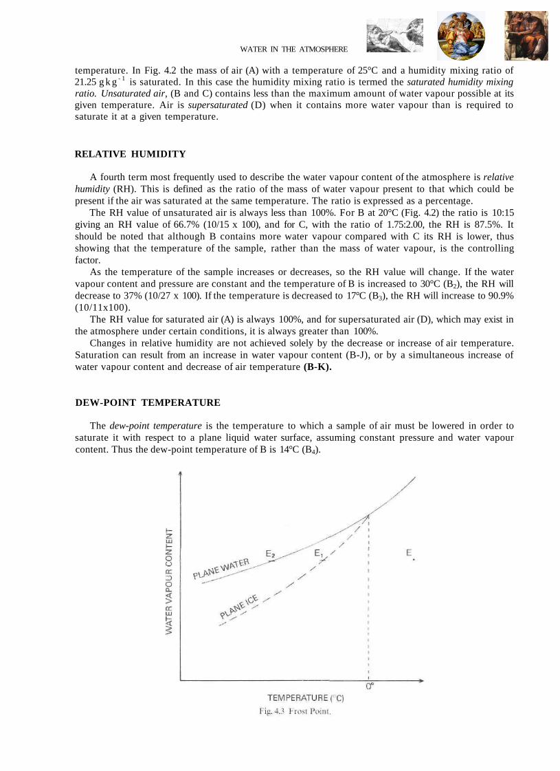
WATER IN THE ATMOSPHERE 21
temperature. In Fig. 4.2 the mass of air (A) with a temperature of 25°C and a humidity mixing ratio of 21.25 g k g - 1 is saturated. In this case the humidity mixing ratio is termed the saturated humidity mixing ratio. Unsaturated air, (B and C) contains less than the maximum amount of water vapour possible at its given temperature. Air is supersaturated (D) when it contains more water vapour than is required to saturate it at a given temperature.
RELATIVE HUMIDITY
A fourth term most frequently used to describe the water vapour content of the atmosphere is relative humidity (RH). This is defined as the ratio of the mass of water vapour present to that which could be present if the air was saturated at the same temperature. The ratio is expressed as a percentage.
The RH value of unsaturated air is always less than 100%. For B at 20°C (Fig. 4.2) the ratio is 10:15 giving an RH value of 66.7% (10/15 x 100), and for C, with the ratio of 1.75:2.00, the RH is 87.5%. It should be noted that although B contains more water vapour compared with C its RH is lower, thus showing that the temperature of the sample, rather than the mass of water vapour, is the controlling factor.
As the temperature of the sample increases or decreases, so the RH value will change. If the water vapour content and pressure are constant and the temperature of B is increased to 30°C (B2), the RH will decrease to 37% (10/27 x 100). If the temperature is decreased to 17°C (B3), the RH will increase to 90.9% (10/11x100).
The RH value for saturated air (A) is always 100%, and for supersaturated air (D), which may exist in the atmosphere under certain conditions, it is always greater than 100%.
Changes in relative humidity are not achieved solely by the decrease or increase of air temperature. Saturation can result from an increase in water vapour content (B-J), or by a simultaneous increase of water vapour content and decrease of air temperature (B-K).
DEW-POINT TEMPERATURE
The dew-point temperature is the temperature to which a sample of air must be lowered in order to saturate it with respect to a plane liquid water surface, assuming constant pressure and water vapour content. Thus the dew-point temperature of B is 14°C (B4).


24 METEOROLOGY FOR SEAFARERS
If the water vapour content of the air remains constant, the RH value decreases during the day as air temperature increases (Fig. 4.2 (B-B2)). The RH will therefore be at a minimum when air temperature is at a maximum (Chapter 3). Thereafter the RH increases as air temperature decreases, and the air may reach its dew-point temperature. If the RH reaches 100%, it will remain at this value until the air temperature begins to increase 1 hour after sunrise.
As the air temperature increases during the day, the air is capable of holding an increasing amount of water vapour, and evaporation occurs if conditions are favourable. However, the increase in air temperature has a greater influence on the RH value than the increase in water vapour content. There is therefore an overall decrease in RH value during the period. If, during the subsequent cooling period, the air temperature decreases below its dew-point temperature, the RH remains at 100% and condensation occurs (Fig. 4.2 (B5-B6-B7-B8)). This explanation has considered only the immediate surface and the air mass above it. However, it should be noted that the movement of air from other areas will also introduce irregularities into the diurnal variation of relative humidity (Chapter 7 and 8).
HYGROMETERS
Hygrometers have been developed to assist in determining the water vapour content of air. The most commonly used hygrometer is Mason's Hygrometer, a dry and a wet-bulb thermometer which are housed in the Stevenson or Marine Screen (Chapter 3). A second form is the whirling psychrometer, or hygrometer, in which the dry and wet-bulb thermometers are fixed in a framework which can be rotated by hand (Fig. 4.7). The wet-bulb thermometer has its bulb encased in muslin. This is kept damp with
distilled water drawn by a wick from a reservoir. Where a platinum resistance thermometer is used this is also encased in muslin.
The working principle of the wet-bulb thermometer in both instruments is that, when ventilated with unsaturated air, water evaporates from the damp muslin, the energy needed (latent heat of vaporization) being drawn from the surrounding air. The air temperature thus decreases, and the

WATER IN THE ATMOSPHERE 25
wet-bulb thermometer records this temperature. The difference between the readings of the dry-and wet-bulb thermometers is called the depression of the wet-bulb, and the lower the RH value the greater will be the depression. If the air has an RH of 100% there will be no depression.
The rate of evaporation of water from the wet-bulb thermometer also depends on the rate of air flow, being 2-4 knots for the Mason's Hygrometer, and at least 7 knots for the whirling psychrometer. Each instrument therefore requires a separate set of hygrometric tables. These tables give values for dew-point temperature, relative humidity, and vapour pressure for each reading of the dry-bulb temperature and depression of the wet-bulb.
It should be noted that, if the wet-bulb reading is below 0°C, it is assumed that the muslin is coated with ice. If supercooled water (water in liquid form at a temperature below 0°C) exists on the bulb, it must be converted to a coating of ice, and the instrument ventilated before a reading is taken.

CHAPTER 5
CLOUDS
INTRODUCTION
Clouds are collections of water droplets or ice crystals, or combination of these two states of water, suspended in the atmosphere. A knowledge of the many types of clouds and their occurrence provide a valuable source of information to the seafarer in forecasting the weather.
CLOUD TYPES
The shapes of cloud within the troposphere may be stratiform (flattened or layered), cumuliform (heaped), cirriform (hair or thread-like), or a combination of these. There are ten basic genera or characteristic forms, and further subdivision into species and varieties can be made. The internationally agreed classification of the ten genera is related to the height of the cloud base above the surface (Table 5.1).
Table 5.1 Cloud genera
Cloud base
HIGH
MEDIUM
LOW
Genera
Cirrus Cirrostratus Cirrocumulus
Altostratus Altocumulus
Stratus Stratocumulus Nimbostratus Cumulus Cumulonimbus
Abbreviation
Ci Cs Cc
As Ac
St Sc Ns Cu Cb
Height of base in kilometres
Tropics
> 6
2-7.5
<2
Mid tats.
> 5
2-7
<2
High lats.
> 3
2 4
< 2
"Alto" identifies the medium level clouds, and "nimbus" implies rain, but other forms of precipitation are possible.
Table 5.2 sets out the salient features of each genus.
ADIABATIC LAPSE RATE
Cloud formation is mainly the result of air ascending and cooling adiabatically. When a parcel of air ascends, the pressure exerted on it by the surrounding atmosphere decreases, so allowing the parcel to expand. In order to do so it requires energy which is derived from the parcel itself, and its temperature therefore decreases. Since air is a poor conductor, it is assumed that no energy is exchanged between the air parcel and the surrounding atmosphere. This process, in which no heat enters or leaves the system, is termed adiabatic from the Greek word meaning "impassable". When an air parcel descends, the reverse
26

CLOUDS 27
Table 5.2 Description of cloud genera
Cirrus (Ci)
Cirrostratus (Cs)
Cirrocumulus (Cc)
A hostrat us (As)
Altocumulus (Ac)
Stratus (St)
Stratocumulus (Sc)
Nimbostratus (Ns)
Cumulus (Cu)
Gumulonimbus (Cb)
High Clouds Detached clouds in the form of white delicate filaments or white or mostly white patches or
narrow bands. These clouds have a fibrous appearance or a silky sheen or both. A transparent whitish cloud veil of fibrous appearance or smooth appearance totally or
partly covering the sky, and generally producing halo phenomena. A thin, white patch, sheet or layer of cloud without shading, composed of very small
elements in forms of grains or ripples merged or separate and more or less regularly arranged.
Medium Clouds A greyish or bluish cloud or layer of striated, fibrous or uniform appearance, totally or
partly covering the sky, and having parts thin enough to reveal the sun at least vaguely. A white or grey, or both white and grey, patch, sheet or layer of cloud, generally composed
of rounded masses or rolls, which are sometimes partly fibrous or diffuse and which may not be merged.
Low Clouds A generally grey cloud layer with a fairly uniform base. When the sun is visible through the
cloud its outline is clearly discernible. A grey or whitish or both grey and whitish patch, sheet or layer of cloud which almost
always has a dark part, composed of rounded masses or rolls, which are non-fibrous, and which may or may not be merged.
A grey cloud layer, often dark, whose appearance is rendered diffuse by more or less continuously falling rain or snow, which in most cases reaches the ground. It is thick enough throughout to blot out the sun.
Detached clouds, generally dense and with sharp outlines, developing vertically in the forms of rising mounds, domes or towers, of which the bulging upper part often resembles a cauliflower. The sunlit parts of these clouds are mostly brilliant white and their bases relatively dark and nearly horizontal.
A heavy dense cloud, with a considerable vertical extent, in the form of a mountain or huge towers. At least part of its upper portion is usually smooth, fibrous or striated, and nearly flattened; this often spreads out in the form of an anvil or vast plume.
Plate
1
2
3
4
5
6
7
8
9 10
11
process occurs and its temperature increases. The rate at which the temperature of the parcel changes with height is termed the Adiabatic Lapse Rate. For a dry air parcel, in which the air is unsaturated, the rate is 9.8°Ckm_1 (usually rounded up to 10.0°Ckm-1). This is the Dry Adiabatic Lapse Rate (D.A.L.R.), which is applicable whether the air parcel is ascending or descending.
An ascending saturated air parcel will cool at the Saturated Adiabatic Lapse Rate (S.A.L.R.), the value of which is less than the D.A.L.R.. During its ascent the volume of the air parcel increases, and its temperature decreases, as for an unsaturated air parcel. As a result some water vapour condenses,


CLOUDS 29
ATMOSPHERIC STABILITY
An assessment of the stability of the atmosphere based on a knowledge of the Environmental, Dry and Saturated Adiabatic Lapse Rates is of considerable value in forecasting cloud development and related weather conditions.
The atmosphere is absolutely unstable when a saturated or unsaturated air parcel, ascending and cooling adiabatically, has a tendency to continue its displacement. In Fig. 5.2(1), an air parcel at level AA has a temperature greater than that of the surrounding atmosphere. It is therefore less dense and, being buoyant, continues to ascend. For a descending parcel, warming adiabatically, its temperature is less than that of the surrounding atmosphere at any given level, and the parcel continues to descend. In an absolutely unstable atmosphere, the E.L.R. is greater than D.A.L.R., which is greater than S.A.L.R. (E.L.R. > D.A.L.R. > S.A.L.R.).
The atmosphere is absolutely stable when any saturated or unsaturated air parcel, ascending and cooling adiabatically, has a tendency to return to its original level. In Fig. 5.2(2), the temperature of an air parcel at level BB is less than that of the surrounding atmosphere. The parcel is therefore denser and tends to return to its original level. A descending air parcel, warming adiabatically, tends to return to its original level, since it is warmer than the surrounding atmosphere. In an absolutely stable atmosphere, the D.A.L.R. is greater than S.A.L.R., which is greater than E.L.R. (D.A.L.R. > S.A.L.R. > E.L.R.).
The atmosphere is conditionally unstable when an unsaturated air parcel, ascending and cooling adiabatically, is at a lower temperature than the surrounding atmosphere at any level. In Fig. 5.2(3), this condition exists at level CC, and the air parcel tends to return to its original level, since it is denser than the surrounding atmosphere. However, at this level a saturated air parcel, which has ascended and cooled adiabatically, has a temperature greater than that of the surrounding atmosphere and continues to ascend. In a conditionally unstable atmosphere, the D.A.L.R. is greater than E.L.R., which is greater than S.A.L.R. (D.A.L.R. > E.L.R. > S.A.L.R.).
The atmosphere is in a state of neutral equilibrium when the E.L.R. equals D.A.L.R., or the E.L.R. equals S.A.L.R.. In each case the air parcel, ascending (descending) and cooling (warming) adiabatically, remains at its new level.
The D.A.L.R. is always constant and, if the S.A.L.R. is assumed to have a fixed value, the E.L.R. will be critical in determining the stability of the atmosphere at a given time. By recording air temperature at increasing heights during a radiosonde ascent, it is possible to establish the E.L.R. for different layers in the troposphere, and thus assess the stability in each of these layers.
FORMATION OF CLOUDS
The stability of the atmosphere plays an important part in the formation and development of clouds and their characteristics, since it controls the method of ascent of an air parcel.
Convection
A convection current, developing at the surface, will ascend cooling adiabatically, and continue to do so as long as it is warmer than the environment (Fig. 5.3(1)). If the air parcel becomes saturated during its ascent it cools at the S.A.L.R.. Water vapour condensing forms water droplets, which are visible in the shape of cumuliform cloud. The base of the cloud is at the condensation level, being the height at

which the convection current begins to cool at the S.A.L.R.. The dimensions of the cloud base partly reflect the dimensions of the convection current, whilst the vertical extent of the cloud depends upon the height to which the current ascends. In these circumstances the atmosphere immediately above the surface is absolutely unstable (E.L.R. > D.A.L.R. > S.A.L.R.), and this condition is termed superadiabatic, and results from the heating of the atmosphere by the surface (Chapter 3).
Cumuliform cloud may be fair-weather cumulus (Plate 9) with limited vertical extent (Fig. 5.3(1)), towering cumulus (Plate 10: Fig. 5.3(2)), or cumulonimbus (Plate 11: Fig. 5.3(3)). A distinctive contrast

CLOUDS 31
exists between the first two and cumulonimbus, as the former have sharp outlines, while the latter has a smooth fibrous or striated upper portion, described as diffuse. A sharp outline denotes a cloud composed of water droplets or supercooled water droplets, which on the periphery of the cloud evaporate into the surrounding unsaturated air. The energy required for evaporation results in a decrease in temperature of the air, which becomes denser and sinks to produce the well-defined edge to the cloud.
Cumulonimbus normally develops from towering cumulus, and the change to a diffuse outline is observed when the water droplets on the upper edge of the cloud change into ice crystals (the cloud has become glaciated). An anvil is formed as the crystals tend to drift into the surrounding atmosphere where they sublimate slowly (Plates 12,13 and 14).
If there is an upper level inversion (Fig. 5.3(4)), cumulus cloud ceases development vertically at this level, but may spread horizontally, forming stratocumulus or altocumulus depending on the height at which the inversion exists (Plate 15).
The development of a cumuliform cloud depends upon a stream of convection currents from the surface. The air parcel concept assumes that the currents retain their identity during ascent, but this is not the case since environmental air will mix with the convection currents, a process called entrainment. This process tends to prevent the initial currents reaching condensation level, but modifies the environmental air through which successive currents ascend, thus allowing the latter to reach greater heights.
The variation of wind direction and speed with height, termed vertical wind shear, may also affect the shape of cumuliform clouds, which may appear to be either more advanced or retarded with increasing height.
On occasions convection currents may generate a funnel shaped cloud, termed a waterspout, which may exist for up to half an hour (Plate 16). A waterspout develops at the base of a cumulonimbus cloud, from which it descends to the surface, and may be appreciably bent by vertical wind shear. Its diameter may vary from a few metres to a few hundred metres and within this area it generates confused seas.
Orographic
Air moving across the surface of the earth will be forced to ascend over a hill or mountain lying in its path, and thus cools adiabatically. The clouds which may form are called orographic and are associated with a stable atmosphere, where air has to be forced to ascend (Fig. 5.3(5)). Cloud may be stratus or nimbostratus, with a base at the condensation level and an upper limit depending upon the height of the barrier (Plate 17). The Tablecloth, a well known example, is a stratus cloud which forms on the windward side of Table Mountain in South Africa.
Dependent upon the distribution of temperature, wind direction and speed with height, a wave motion may be generated downwind of a physical barrier. This condition can be observed by the pressence of lens-shaped or lenticular clouds, which indicate where the air is rising on each successive wave crest (Plate 18). These clouds are often visible at substantial distances downwind of the barrier.
In a conditionally unstable atmosphere orographic conditions play an important part in forcing an unsaturated air parcel to ascend (Fig. 5.3(6)). The parcel will cool adiabatically and become saturated, and further forced ascent and cooling at the S.A.L.R. may eventually result in the air parcel (Y) having a temperature greater than that of the surrounding air. The parcel will then rise spontaneously until its temperature is the same as that of the surrounding atmosphere. Cumulus or cumulonimbus cloud develops.
Turbulence
Turbulence, by redistributing the water vapour uniformly and affecting the E.L.R. within the turbulent layer, can cause cloud formation (Chapter 3). Above a certain height within the layer, condensation occurs and stratus or stratocumulus cloud develops (Fig. 5.3(7)). Turbulence is therefore another process which can force air to ascend in a stable atmosphere. Although it is only effective to a limited height, the horizontal area covered by the cloud is usually extensive over land and sea.
Finally, it should be noted that clouds also form as a result of large scale vertical air motion in frontal depressions (Chapter 8).
\y

CHAPTER 6
PRECIPITATION AND FOG
FORMS OF PRECIPITATION
Precipitation is the deposit on the earth's surface of water in liquid or solid state or a combination of both. The principal forms are:
Drizzle — Water droplets with diameters between 200 urn and 500 um. Rain—Water droplets with diameters exceeding 500 urn. Snow or Snowflakes—Small ice crystals or aggregates of ice crystals. Hail—Balls of ice of varying size. Sleet—Mixture of rain and snow.
Ice pellets, prisms or granular snow also occur. Usually, but not always, precipitation is associated with a cloud. On occasions it can be seen leaving the base of a cloud in vertical or inclined trails which do not reach the surface, which are termed fallstreaks or virga.
DEVELOPMENT
Cloud droplets have diameters of the order of 20 um compared with drizzle droplets of 200 urn or more. Investigations have established that the increase in size of droplets is not caused by condensation

PRECIPITATION AND FOG 33
within the cloud. In a cloud composed entirely of droplets whose temperatures are greater than 0°C the theory of coalescence applies. The size of a cloud droplet is directly related to the size of the condensation nucleus on which it forms. A large droplet has a greater speed of descent compared with a smaller one, and it is therefore possible for the former to collide with the latter lying in its path and they coalesce (join together).
As the larger droplet gathers momentum further collision and coalescence occurs. Eventually the droplet leaves the cloud when its size is such that its speed of descent exceeds the upward movement of air, or updraught, within the cloud. The droplet may decrease in size through evaporation before it reaches the surface, depending upon the relative humidity of the air below the cloud base.
The clouds in which this process occurs are termed "warm" clouds, and the type of cloud determines whether drizzle or rain is experienced. For example, stratus produces drizzle, whereas nimbostratus and cumuliform clouds produce rain (Fig. 6.1). Rain drops from cumulus and cumulonimbus clouds can be very large as a result of the concentration of water droplets within the cloud, and the increased frequency of collision due to smaller droplets being lifted by the updraught.
Fig. 6.2 Ice crystal development.
In a "cold" cloud, in which the air temperature is less than 0°C in part if not throughout the cloud, the Bergeron-Findeisen theory applies. In these clouds the water droplets are supercooled. The development of ice crystals from these droplets depends upon the presence of freezing nuclei, which have a crystalline structure similar to that of the hexagonal form of ice. Many of these nuclei are introduced into the atmosphere from the surface, and each type of nucleus has a threshold temperature below which a supercooled water droplet will freeze on coming into contact with it. An important nucleus is the clay mineral kaolinite whose threshold temperature is — 9°C. With decreasing air temperature different types of freezing nuclei become active, and at — 22°C and below a cloud is composed entirely of ice crystals. A newly formed ice crystal is surrounded by air (Fig. 6.2 (A1) which is saturated with respect to a plane water surface, and supersaturated with respect to a plane ice surface. Water vapour will therefore sublimate directly onto the ice crystal which increases in size. The surrounding air then becomes unsaturated with respect to a plane water surface (A2), thus the supercooled water droplets present decrease in size through evaporation. As this process is repeated the crystal grows. Air currents within the cloud may cause the crystal to fragment, and each fragment then forms a further nucleus, thus increasing the number of crystals within the cloud. Collision and aggregation (joining together) of ice crystals may occur, particularly between 0°C and — 5°C, resulting in large snowflakes.
When the snowflake is of such a size that its speed of descent overcomes the updraught it will leave the base of the cloud. Snow occurs when the surface air temperature is below 0°C, but between 0°C and 3°C some of the snowflakes melt, resulting in sleet (Fig. 6.1). When an ice crystal descends into the lower part of the cloud where the temperature is greater than 0°C, it melts forming a water droplet which then grows through collision and coalescence, and reaches the surface in the form of rain. These processes can occur in cumulus, cumulonimbus and nimbostratus clouds (Fig. 6.1).

34 METEOROLOGY FOR SEAFARERS
Fig. 6.3 Hailstone. Cross section showing alternating clear and opaque ice.
Hailstones
Hailstones are associated with cumulonimbus clouds, and are usually spherical, with diameters ranging from 5 mm to 50 mm or more. The structure of each stone is a series of concentric shells of alternating clear and opaque ice (Fig. 6.3), which is the result of low and high air concentrations respectively. In a cumulonimbus cloud the strong updraught lifts water droplets into its upper part where they freeze, and become the nuclei of hailstones. Each hailstone may then increase in size through collision and accretion (joining together) with water droplets. The developing hailstone then descends and, if it remains within the cloud, rejoins the updraught. This process may be repeated several times until its speed of descent overcomes the updraught and it leaves the cloud (Fig. 6.4).

PRECIPITATION AND FOG 35
OBSERVATION
A number of terms are used for observing purposes to describe the precipitation reaching the surface:
Showers—From convective clouds of short duration in the form of rain, snow, hail or sleet with rapid fluctuation of intensity (Plate 19).
Intermittent precipitation —From stratiform clouds, when there are breaks in the precipitation within the past hour.
Continuous precipitation—From stratiform clouds, when it has lasted for at least an hour without a break.
Precipitation whether from cumuliform or stratiform clouds may be described as slight, moderate or heavy. Each term indicates the amount, as a depth in millimetres, reaching the surface during one hour. Particular values are noted in observers' handbooks.
Thunderstorms, which are flashes of lightning from electrical discharges and thunder, may be associated with very heavy, or violent, showers of hail or rain from cumulonimbus cloud (Plate 20). Simultaneously there is an increase in surface wind speed and pressure, and a decrease in air temperature, which together reflect the downdraught developed in the cloud as a result of the precipitation.
Drizzle or rain may freeze on coming into contact with the surface of the earth or any object standing above it, when it is termed freezing drizzle or freezing rain. The ice formed is termed glazed frost, or black ice when encountered on roads, and at sea, icing or ice accretion.
VISIBILITY
For meteorological purposes horizontal visibility is defined as the greatest distance at which an object with specified characteristics can be seen and identified by the unaided eye in daylight. At night it is assumed that the illumination of the object is raised to normal daylight level.
Visibility is assessed by viewing the horizon through 360° and recording the shortest distance. Land observing stations use objects at known distances in daytime and a visibility meter at night, thus making it possible to provide accurate visibility ranges:

36 METEOROLOGY FOR SEAFARERS
Visibility is reduced by the suspension of liquid or solid particles in the atmosphere. If the visibility is reduced to less than 1 km as a result of water droplets, the condition is termed fog, and if 1 km or greater it is termed mist.
If visibility is reduced by the presence of solid particles the condition is termed haze, for which there is no upper limit to the value of the visibility range. When dust and sand are lifted into the atmosphere resulting in a visibility range of less than 1 km, the condition is termed a duststorm or sandstorm, and above this range a dust or sand haze. Smoke, whether from manmade sources or volcanic activity, may also cause reduced visibility.
FOG
Fog develops for a variety of reasons and a number of types can be identified:
Advection fog Sea Smoke Radiation fog Frontal fog (see Chapter 8)
Advection Fog
Advection fog develops as a result of a mass of warm air, with a high relative humidity value, moving horizontally (hence the term advection) over a cooler surface, whose temperature is below the dew-point temperature of the air. When, as a result of conduction aided by turbulence, the air is cooled below its dew-point temperature, water vapour condenses, the water droplets producing the mist/fog condition.
This type of fog forms and persists under a wide range of wind speeds. The degree of turbulence dictates the maximum height to which the air is cooled, the height increasing with increasing wind speed. Thus the temperature gradient between air and surface in conjunction with the degree of turbulence determines the likelihood of advection fog. Low wind speeds provide more favourable conditions but, with a steep temperature gradient, advection fog can develop in gale force winds. However, higher wind speeds associated with small temperature gradients are more likely to produce low level stratus cloud, as the effective cooling of the air by the surface is less and is spread over a greater height. The lower troposphere normally becomes stable since cooling of the air decreases the environmental lapse rate.
At sea advection fog, termed sea fog, occurs at certain times of the year (Fig. 6.5). In northern latitudes, the Grand Banks of Newfoundland and the North Pacific zones are notorious particularly in July, when warm air from the south-west and south pass over the cold waters of the Labrador, and the Oyo Shio or Aleutian Currents respectively. Sea fog in these areas can persist for extended periods and will only disperse when either the wind speed increases, or its direction changes. Sea fog also occurs in lower latitudes during the summer in the region of the cold California, Canary, Peru and Bcnguela Currents.
Sea fog not only develops where cold currents exist, but also where there are favourable conditions of wind speed, air and sea surface temperatures. Examples are the spring and early summer fogs of the Western Approaches to the British Isles, where the south-westerly warm air stream from the Azores moves over the sea which, at this time of the year, is at its lowest temperature (Plates 21, 22 and 23). In the North Sea, sea fog develops during the summer when warm north-east, east and sometimes southeasterly winds from Europe pass over the colder sea surface. Along the east coast of the British Isles this sea fog is called haar or sea fret.
On land, warm air moving over cold surfaces may also produce advection fog. In the British Isles this usually occurs in winter through advection of a warm air stream from the Azores. At this time of year advection fog also develops over the southern and eastern areas of the United States of America, when warm air is advected from the Gulf of Mexico and the Bermuda region.
Sea fog is a frequent threat to the seafarer and its prediction is therefore important. As sea and dew-point temperatures are critical in its formation, their observation at frequent intervals is recommended, and should be recorded in graphical form (Fig. 6.6). By drawing straight lines to establish the trend of each temperature, it is possible to determine the point of intersection (F), which indicates when fog may be encountered.
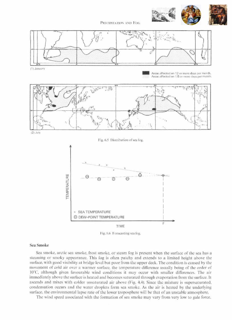

38 METEOROLOGY FOR SEAFARERS
Higher speeds are more favourable when the temperature difference is small, as they ensure a continuous supply of cold air immediately above the surface.
Off the east coasts of the North American and Asian continents sea smoke occurs during the winter months, when cold air from the continent passes over estuaries, coastal waters, (e.g. St. Lawrence Seaway—Plate 24) and adjacent ocean areas. During winter it occurs in the Baltic Sea which is surrounded by a colder land mass, and in higher latitudes it is associated with cold winds from the Arctic Basin and the ice covered sea areas to the south. In lower latitudes it occurs occasionally in the Gulf of Mexico and off Hong Kong.
As the air temperature is low, the droplets forming sea smoke are often supercooled, and icing occurs when the droplets freeze on contact with those parts of a vessel which are below 0°C.
Radiation Fog
Radiation fog is a land based fog in its development. Clear skies, a high relative humidity, very low wind speeds, and a relatively long period during which the air can cool, are the most suitable conditions for its formation. The clear sky condition allows the maximum loss of long wave radiation from the surface during the night. Surface temperatures decrease rapidly, and the air immediately above is cooled through conduction aided by turbulence. Once the air is cooled below its dew-point temperature, condensation occurs and radiation fog is produced. Since the length of the cooling period is critical, radiation fog is more common during the autumn and winter in mid and high latitudes, e.g. in the British Isles. The cooling of the air by the surface results in a progressive decrease in the environmental lapse rate and the atmosphere eventually becomes stable. A ground level inversion may well develop (Fig. 3.5(2)).
Although conditions favourable for the formation of radiation fog may exist over the sea, the diurnal ranges of both sea surface and air temperatures are too small for the air to be cooled below its dew-point temperature, and therefore no condensation occurs. Radiation fog will affect visibility at sea if it drifts over estuaries and coastal waters as a result of light offshore winds. The air will then be heated by the warmer water over which it passes and, as its temperature increases, the fog droplets will gradually evaporate.
Radiation fog may disperse as a result of an increase in land surface temperature during the day, since the surface heats the air immediately above, and lowers its relative humidity. An increase in wind speed can also cause dispersal since it overturns the air. The RH is thus decreased as a result of mixing with unsaturated air. As the increase in land surface temperature is small during the winter day, fog may persist on land and continue to affect estuaries and coastal waters.
In tropical regions, radiation fog is comparatively rare at sea level, but may be experienced over river estuaries during the early hours of the morning. The fog develops during the night over adjacent river banks, where the air has a high relative humidity due to the presence of open water. Similar conditions also apply in swamp and marsh areas.
HAZE
Development of haze on land can often be related to the diurnal cycle of air and surface temperatures. With a significant increase in surface temperature during the day, convection and turbulence increase and dust particles are raised from the surface. Thus the visibility decreases progressively through the day as an increasing number of particles remain suspended in the atmosphere. The condition is more marked when the E.L.R. limits the ascent of air to the lower part of the troposphere, thus causing a rapid increase in the concentration of dust particles. During the night the particles settle onto the surface, and visibility is improved in the early part of the day.
At sea, haze often the result of movement of dust and sand particles from land. A particular example occurs, usually between November and May, off the north-west coast of Africa, where large quantities of dust from the Sahara are blown off-shore by the local wind, the Harmattan. A similar condition occurs in the Gulf during the summer with the Shamal, a north-westerly wind which collects dust from the desert. Salt particles, which are potential condensation nuclei, may also produce haze at sea when the RH value of the atmosphere is too low for water droplets to develop.

CHAPTER 7
WIND
DEFINITION
Wind is defined as the horizontal movement of air across the surface of the earth. The direction from which it blows and its speed are its important characteristics. Wind direction is related to True North (360°(T)), and it is recorded and coded in meteorological reports to the nearest 10°(T) clockwise from this direction. A wind blowing from the East will be recorded as 090°(T), whilst no wind or calm condition is recorded as 00. Wind speed is currently expressed in knots or metres per second.
The wind is rarely steady in direction and speed for any prolonged period, and thus a mean value over a ten minute period is assessed for observational purposes. A gust, an increase, and a lull, a decrease in speed about the mean value may well be experienced. If, during the ten minute period, the wind speed changes by 10 knots or more, and the new speed is maintained for more than 3 minutes, then the new speed is recorded. A squall is a prolonged gust with a duration of more than one minute and an increase in speed of at least 16 knots, or three steps on the Beaufort Scale (see below), its speed being Force 6 or greater.
OBSERVATION
Land Observations
The standard observing height for wind is 10 metres above the surface. A wind vane, used to indicate direction, and an anemometer, for speed are mounted together on a mast where there is a free flow of air across the surface (Fig. 7.1). The operation of the wind vane is dependent upon the pressure of the wind


WIND 41
acting on the vertical flat plate (A) so that the bar (B), which rotates horizontally and freely about its centre, is aligned with the direction of the wind. The other end of the bar is the pointer which, indicates the direction from which the wind blows. The position of the pointer can be registered on a digital or dial display, and can be continuously recorded on a chart, often sited at some distance from the mast itself.
The anemometer consists of three hemispherical cups with beaded edges held vertically on horizontal bars of equal length, which radiate at 120° apart from a central pivot (Fig. 7.1). The cups are designed to achieve a turbulent-free flow of air. As the pressure of the wind on the concave side of the cups is greater than on the convex side, the cups rotate and operate a small electrical generator which produces a current. The value of the current is related to the speed of rotation and hence the wind speed. Thus the wind speed can be registered in the same way as the wind vane data.
Sea Observations
In the 19th Century, Admiral Beaufort introduced the Beaufort Scale, a scale from 0 12 called Beaufort Force numbers, each number corresponding to a range of wind speeds. Originally expressed in terms of the effect on a man of war and the setting of sails, today it is based on the state of the sea (Table 7.1 and Plates 30-42)). The sea criteria are the wind waves which are generated by the wind which has been in existence for a reasonable period, and having an adequate fetch (the distance of open water over which the wind has blown). However, the wind is not the only factor influencing the sea state, and allowances should be made for tides, currents, depth of water and precipitation, where these are seen to affect the sea state. Tides opposing the direction of the wind waves will create more "lop", and an overestimate of wind speed is possible. Heavy precipitation flattens the sea and may lead to an underestimation. Wind direction is established by observing the direction from which the wind waves advance.
Waves generated by winds at some distance from, or at some time previously at the point of observation also affect the sea. This wave motion is called swell, and is excluded when recording the Beaufort Force. Swell, in contrast to wind waves, has a long and generally low regular wave form (Plate 43). It may be at any angle to the wind waves, and more than one swell may exist at the same time. Thus swell gives a useful indication of conditions existing, or which existed at some distance in the direction from which it is coming. Swell generated by wind conditions in the Southern Oceans has often been observed in the Western Approaches to the British Isles. The presence of swell may also be one of the earliest indications of a tropical cyclone.
For meteorological purposes the period and height of wind waves and swell, and the direction from which the swell is coming are recorded. The period of a wave is the time taken for the passage of two successive crests past a point selected by the observer. The height of the wave is the vertical distance between the bottom of the trough and the top of the crest. As waves normally occur in groups, the height and period are assessed by observing two or more of the relatively large waves in each group, until at least ten such waves have been observed. The period is the average value of the recorded times, and the height is the average value of the heights observed. Table 7.1 includes a guide to the classification of wind waves related to wind speed. The following table is a guide to the classification of swell waves:
Conditions at sea often preclude an accurate observation of the sea state and the use of the Beaufort Scale. On these occasions the wind vane and anemometer, funnel smoke, and flags can be observed to establish the relative wind speed and direction. As the true wind is required, it is derived using a vector

42 METEOROLOGY FOR SEAFARERS
triangle (Fig. 7.2). The vessel's course reversed and the relative wind direction are plotted relative to true north, using the vessel as the focal point of the triangle. The length of each line is scaled to represent speed. The third side of the triangle gives the true wind direction and speed.
N
If there is no relative wind, the vessel's course and the speed reversed is the same as the true wind direction and speed (Relative Wind—00: Course 090°(T)—10 knots: True Wind 270°(T)—10 knots).
If the relative wind is from the bearing on which the ship is steering, the direction of the true wind is the vessel's course, and its speed is the difference between the vessel's speed and the relative wind speed (e.g. Relative Wind 270°(T)—20 knots: Course 270°(T)—10 knots: True Wind 270°(T)—10 knots).
The siting of wind vanes and anemometers on a vessel pose problems in providing a free flow of air. The standard height of 10 metres is rarely practicable if the effect of the superstructure is to be avoided, and a compromise has to be accepted, with the consequent inaccuracy of readings on some bearings.

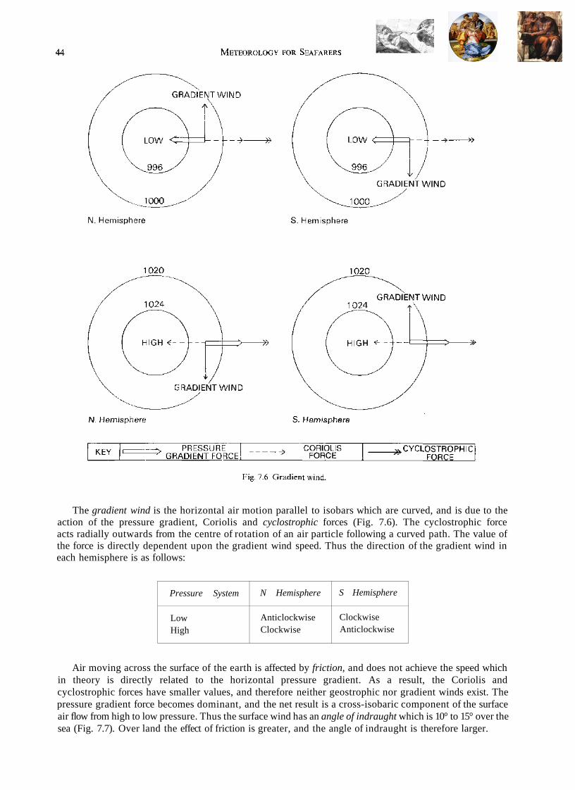
The gradient wind is the horizontal air motion parallel to isobars which are curved, and is due to the action of the pressure gradient, Coriolis and cyclostrophic forces (Fig. 7.6). The cyclostrophic force acts radially outwards from the centre of rotation of an air particle following a curved path. The value of the force is directly dependent upon the gradient wind speed. Thus the direction of the gradient wind in each hemisphere is as follows:
Pressure System
Low High
N Hemisphere
Anticlockwise Clockwise
S Hemisphere
Clockwise Anticlockwise
Air moving across the surface of the earth is affected by friction, and does not achieve the speed which in theory is directly related to the horizontal pressure gradient. As a result, the Coriolis and cyclostrophic forces have smaller values, and therefore neither geostrophic nor gradient winds exist. The pressure gradient force becomes dominant, and the net result is a cross-isobaric component of the surface air flow from high to low pressure. Thus the surface wind has an angle of indraught which is 10° to 15° over the sea (Fig. 7.7). Over land the effect of friction is greater, and the angle of indraught is therefore larger.

W I N D 45
Fig. 7.7 Angle of indraught.
Buys Ballot's Law
In 1857, Buys Ballot formulated a law identifying the relationship between wind and pressure distribution. The law states that if an observer has his back to the wind, then low pressure will be to the left in the northern hemisphere and to the right in the southern hemisphere. It follows that high pressure will lie on the right in the northern and on the left in the southern hemisphere (Fig. 7.8). Under certain circumstances the number of points of the compass to the right or left of the wind in which the low pressure centre lies is important, particularly when assessing the position and movement of tropical cyclones (Chapter 9).
Fig. 7.8 Buys Ballot's Law.

46 MKTFOROLOGY FOR SEAFARERS
Surface Wind
Although a geostrophic wind does not exist at the surface, the concept is used in determining surface wind speeds. Facsimile meteorological charts may have geostrophic wind scales specifically related to the projection and scale of each chart. Fig. 7.9 is an example of the use of the scale in determining surface wind speed at 48.5°N. The perpendicular distance between isobars (AB) is measured and plotted on the scale. The geostrophic wind speed of 12 knots (C), found by interpolation, is reduced by one third to allow for friction, and the predicted surface wind speed is thus 8 knots.
Wind direction is determined by Buys Ballot's Law and applying an angle of indraught of 10° to 15°. In the example (Fig. 7.9(2)), with low pressure to the north and the isobars lying approximately WSW—ENE, the wind is from the south-west.

WIND
SEA AND LAND BREEZES
47
The seafarer frequently encounters local wind conditions in coastal waters resulting from heating and cooling of adjacent land and sea surfaces. Such conditions also occur over comparatively large areas of water inland (e.g. The Great Lakes).
During the day, the land surface temperature increases more rapidly than that of the sea surface (Chapter 3). Air temperature above the land is therefore higher, and the vertical motion of the air through convection modifies the pressure gradient in the horizontal plane (1-2) (Fig. 7.10). As the pressure above the land (1) becomes greater than that over the sea in this plane, so the air moves towards lower pressure (2). The surface air pressure on land (4) then decreases, and air moves from the sea (3) to land (4). Thus during the day a sea breeze blows onshore, which may be felt for some distance inland, and an offshore wind blows at some 1000 metres above the sea. The sea breeze gradually increases in speed as the land surface temperature increases, and reaches a maximum by mid-afternoon. When the sky is clear a large amount of solar radiation reaches the surface and the wind speed will be at its maximum (mid-latitudes—Force 3; low latitudes—Force 5).
Fig. 7.10 Sea breeze.
The sea breeze has a considerable influence on weather conditions at the coast and for some distance inland. As the sea breeze is relatively cool, coastal zones experience lower air temperatures compared with those inland. The relative humidity value at the coast is higher than inland, and increases during the afternoon when the breeze reaches its maximum speed. This condition contrasts with diurnal variation of relative humidity noted in Chapter 4. The leading onshore edge of the sea breeze is often marked by a line of cumuliform (convective) cloud, which may result in precipitation, particularly in tropical areas.
By contrast the land breeze which develops during the night is slight, reaching Force 1-2. With clear skies the radiative cooling of the land surface is at a maximum, but the sea surface temperature decreases slowly (Chapter 3). Above the land the air cools, becomes denser (5), and flows downslope towards the sea (6), hence creating the land breeze (Fig. 7.11). The air, heated by the warmer sea surface, ascends (7) and then moves towards the shore (8). Land breezes are normally evident by midnight local time, but on occasions may not develop until the early hours of the morning. It should be noted that the small temperature difference at night between land and sea surfaces, and the topography of the land, both influence the speed of the land breeze. In tropical areas the convective process (6 -> 7) is marked by the development of cumuliform cloud over the sea.
HIGH
LOW
LAND
It is worth noting that both land and sea breezes are caused by local pressure gradients and flow down the gradient. In mid-latitudes the wind may eventually orientate itself parallel to the coastline, reflecting the influence of the Coriolis force on a well developed local system.

48 METEOROLOGY FOR SEAFARERS
KATABATIC AND ANABATIC WINDS
Katabatic (downslope) winds affect sea conditions off mountainous coastal areas, particularly the Norwegian fjords and the ice covered regions of Greenland and Antarctica. They develop at night when there are clear skies, a general slack pressure gradient, and rapid radiative cooling of the land. The air at X (Fig. 7.12) adjacent to the slope, becoming cooler and therefore denser than the air which is further away at the same level (Y), descends forming the katabatic wind. On reaching the foot of the slope the wind moves out to sea. Adiabatic warming of the air during descent is counteracted by conduction as it is in continuous contact with the colder mountain slope. When the slope is covered with ice or snow, which are effective insulators, very limited conduction takes place between the slope and the upper surface of the ice or snow cover. Thus during the cooling period overnight the upper surface experiences a more rapid decrease in temperature than that of a bare slope. Under such conditions, the adjacent air, becoming very cold and dense, descends at a speed which can reach gale force conditions.
During the day an anabatic wind develops. With clear skies the slope absorbs solar radiation and heats the air (P) directly in contact. This air then flows up the slope, as it is at a higher temperature than the air (Q) further away at the same level (Fig. 7.13). The air moving up the slope is subject to expansion and therefore cooling. The contact maintained with the warm slope ensures its continued ascent, with a maximum speed during mid-afternoon. Anabatic winds occur in the Alps in summer months when there is generally a slack pressure gradient.
Fig. 7.12 Katabatic wind. Fig. 7.13 Anabatic wind.
The need for seafarers to understand land and sea breezes is clear. Sea breezes can reach significant speeds which, combined with current and tide may create hazardous conditions. Sailing directions should always be consulted.


50 METEOROLOGY FOR SEAFARERS
At 60°N and S two masses of air having different temperatures converge. The boundary between these masses is called a frontal zone or frontal surface, and where it intersects the surface of the earth it is called a front (Fig. 8.2). The frontal zone is inclined at an angle to the surface with the warm air tending to rise over the cold air.
The transfer of energy by the general circulation is related to the net radiation balance of the earth/atmosphere system, the balance being the difference between the total incoming solar radiation and outgoing terrestrial radiation. Annually there is a surplus of energy between 40°N and 40°S and a deficit in higher latitudes. However, the amount of energy transferred varies with the time of year.
Some of the major features of the general circulation can be identified on surface synoptic charts. Fig. 8.3 is a typical example for the North Atlantic area encompassing the temperate (40°N-66°N), parts of

TEMPERATE AND POLAR ZONE CIRCULATION 51
the subtropical (23°N-40°N), and the polar zones (66°N-90°N). While the subdivision into zones may assist in the analysis of atmospheric features, it must not be forgotten that it is a manmade convention.
Pressure systems in temperate and polar zones play a critical part in determining weather and sea state conditions, and an understanding of the significance of the features on synoptic and prognostic (forecast) charts and in weather bulletins is essential.
FRONTAL DEPRESSIONS
A frontal depression is characterized by having a surface pressure distribution marked by one or more isobars enclosing an area of low pressure. The value of the pressure at the centre, which varies throughout the life cycle of the depression and from one depression to another, generally ranges between 950 hPa and 1020 hPa. A depression having several isobars and a central pressure value below 950 hPa is termed a deep depression.
Most frontal depressions develop on a frontal zone (Fig. 8.4). Polar fronts are boundaries between polar and tropical air; arctic fronts between arctic and polar air; antarctic fronts between antarctic and polar air; the Mediterranean front between polar and tropical air. The mean positions of these frontal zones are shown in Fig. 8.4 for January and July. In January the polar fronts in the southern hemisphere are aligned approximately east-west. In contrast the polar fronts in the northern hemisphere are aligned with the eastern coastlines of North America and Asia, partly reflecting the contrasting influence of land and sea. In the Mediterranean the contrast in air masses is apparent in January, but scarcely exists in July when there is no frontal zone. In July frontal zones in the northern and southern hemispheres lie approximately east-west.
(1)January
(2) July Fig. 8.4 Mean position of frontal zones.


TEMPERATE AND POLAR ZONE CIRCULATION 53
Life Cycle of a Frontal Depression
The formation, development and decay of a frontal depression, whose life cycle may vary in length from three to seven days, can be illustrated by a series of plan diagrams of the system at the surface of the earth (Fig. 8.5(1) to (6)).
Frontogenesis
The progressive separation of isobars indicates a decrease in pressure at a point on a frontal zone (Fig. 8.5(1) and (2)). A wave appears on the front and, if unstable, it continues to develop. The centre of low pressure is at the apex of the wave, and the surface air circulation develops a typical anticlockwise (northern hemisphere) and inward movement. Sections of the original front are now identified as the warm or cold front with an intervening warm sector (Fig. 8.5(3)). This process is termed frontogenesis. During these initial stages the amplitude of the wave increases, and the depression moves rapidly eastwards parallel to the isobars of the warm sector, sometimes at speeds of over 40 knots (Fig. 8.5(3) and (4)). The position of the warm front at the surface marks the point at which warm air replaces cold air; the position of the cold front where cold air replaces warm air.
Within 24 hours of the initial wave formation, the depression usually reaches maturity (Fig. 8.5(4)) and its central pressure value has decreased (the depression has deepened). As the depression deepens so the pressure gradient becomes steeper and the wind speeds increase, this process continuing into the early stages of occlusion (see below).
Frontolysis
The speed of advance of the cold front of a depression is greater than that of the warm front, hence the area of the intervening warm sector diminishes. As the warm sector is progressively lifted off the surface from the centre of the depression outwards, an occluded front develops (Fig. 8.5(5)). The depression begins to fill, its central pressure value increasing, and simultaneously wind speeds decrease as the pressure gradient slackens. The speed of advance of the depression decreases and it may eventually become stationary, the occluded front pivoting around its centre (Fig. 8.5(6)). Eventually the weak low pressure area and occluded front fade. The process from initial occlusion to the final fading of the front is termed frontolysis.
Fig. 8.6(1) Synoptic chart—1200 UTC, Day 1.

The life cycle of a frontal depression can be observed by studying a series of synoptic or prognostic surface charts. In Fig. 8.6(1)—(3), covering a period of 48 hours, depression A develops on the polar front and moves NNE, deepening as the amplitude of the wave increases.

TEMPERATE AND POLAR ZONE CIRCULATION 55
(2) Depression fully developed - plan v iew
(3) Elevation through AD (4) Occlusion - plan view J - J e t stream
Fig. 8.7 Polar front jet stream and a frontal depression.
Jet Stream
If a depression is to develop, the air flow in the upper troposphere must be divergent. This divergent flow is associated with a jet stream, a fast moving current of air with strong lateral and vertical wind shears which is located immediately below the tropopause. Fig. 8.7 shows the relationship between the polar front jet stream and a frontal depression during the life cycle of the latter.
Anafronts and Katafronts
Within a frontal depression the warm air usually ascends relative to cold air. This movement is marked by the presence of active warm and cold fronts termed anafronts. The clouds which develop are shown in the elevation in Fig. 8.8(2) corresponding to line AD in Fig. 8.8(1). On occasions the warm air may descend relative to the cold air, and a relatively inactive front termed a katafront exists, with limited low level stratiform cloud.

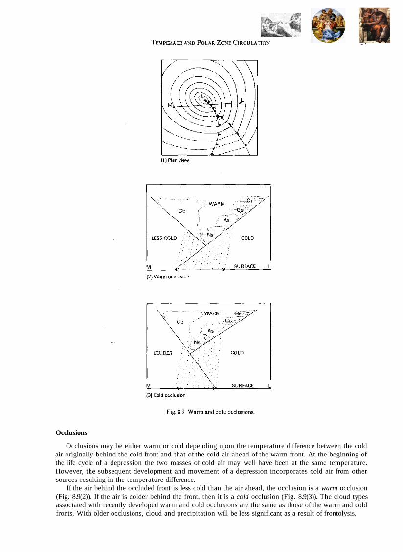
Occlusions
Occlusions may be either warm or cold depending upon the temperature difference between the cold air originally behind the cold front and that of the cold air ahead of the warm front. At the beginning of the life cycle of a depression the two masses of cold air may well have been at the same temperature. However, the subsequent development and movement of a depression incorporates cold air from other sources resulting in the temperature difference.
If the air behind the occluded front is less cold than the air ahead, the occlusion is a warm occlusion (Fig. 8.9(2)). If the air is colder behind the front, then it is a cold occlusion (Fig. 8.9(3)). The cloud types associated with recently developed warm and cold occlusions are the same as those of the warm and cold fronts. With older occlusions, cloud and precipitation will be less significant as a result of frontolysis.

58 METEOROLOGY FOR SEAFARERS
Weather Conditions
The wind, air temperature and precipitation associated with frontal depressions are of particular concern to the seafarer. The sequence of weather will depend on the position of the observer relative to the centre of the depression, and the following tables are a guide:
Table 8.1 Weather sequence of a frontal depression to the south of the observer in the N. Hemisphere (Fig. 8.8(1) and (3)).
Element
Pressure Wind Temperature Cloud Weather Visibility
Sequence
Decreases then increases Backs and increases then decreases Steady, but may decrease when wind backs to N and NW Ci, Cs, As, Ns, As Fine, followed by rain increasing, then decreasing Good, deteriorating then improving
Table 8.2 Weather sequence of a frontal depression to the north of the observer in the N. Hemisphere (Fig. 8.8(1) and (2)).
Element
Pressure
Wind
Temperature
Cloud
Weather
Visibility
Sequence
In advance of warm front
Decreases
Increasing may back
Increases
Ci, Cs, As, Ns
Fine, then rain increasing
Fine, then deteriorating
At warm front
Stops decreasing
Veers and sometimes decreases
Increases
Ns
Rain almost or completely stops
Poor, frontal fog
In warm sector
Little change
Steady
Steady
St
Cloudy, drizzle
Poor, advection fog
At cold front
Rapid increase
Veers, squally
Decreases
Cu,Cb
Hail, rain, thunder, lightning
Poor
To rear of cold front
Increases
May veer further and decreases
Steady, may decrease when wind veers further
Cu,Cb
Showers
Improves, good except in showers
The following comments amplify Tables 8.1 and 8.2:
(a) If the course of the observer is westwards then the duration of events will be shorter. (b) Absolute values of pressure, wind speed and temperature, are not given as these will depend upon
the particular frontal depression. (c) Wind direction:
(i) Backing—the wind direction changes anticlockwise e.g. East through North to West. (ii) Veering—the wind direction changes clockwise e.g. East through South to West.
(d) Rain. The term used includes rain, sleet or snow. (e) The development of frontal fog is due to the evaporation of rain as it passes through the cold air
beneath the frontal surface. As a result the cold air becomes saturated and condensation occurs.
The sequence of weather for cold and warm occlusions in the northern hemisphere is given below:

TEMPERATE AND POLAR ZONE CIRCULATION 59
Table 8.3 Weather sequence of cold and warm occlusions in the N. Hemisphere (Fig. 8.9).
Element
Pressure
Wind
Temperature
Cloud
Weather
Visibility
Cold
Warm
Cold
Warm
Sequence
Ahead of occluded front
Decreases
Backs
Decrease
Increase
Ci, Cs, As, Ns
Precipitation near front
Fine, then precipitation becoming heavy
Deteriorates
At occluded front
Stops decreasing
Veers
Decrease
Increase
Ns,Cb
Heavy precipitation
Precipitation decreasing
Generally poor
To rear of occluded front
Increases
May continue to back; decreases
Steady
Steady
Cb clearing
Heavy precipitation then decreases
Precipitation ceases
Improves
A number of local winds in the Mediterranean are associated with the passage of depressions eastwards (Fig. 8.10). The Scirocco, seldom noticeable in the winter, is a warm southerly wind from the Sahara desert. Initially hot and dry, it may become humid after a sea passage and low level stratus cloud develops. If its speed is high it transports dust, resulting in low visibility and subsequently red rain. Over Egypt the wind is known as the Khamsin.
The Vendavales occurs in the Western Mediterranean, particularly in late autumn and early spring. It is a strong south westerly wind with associated thunderstorms. In contrast the Levanter is an easterly wind occurring in the same area between June and October, with orographic cloud developing over the Rock of Gibraltar.
The Mistral, a cold north to north-westerly wind, occurs in the Gulf of Lions mainly during the winter. It develops as a result of the transit of a depression eastwards over the sea with high pressure over North-West France. The Bora, a cold dry north-easterly wind, occurs in the Adriatic during the winter months, and is associated with high pressure over Central Europe and depressions to the south.
Fig. 8.10 Local winds of the Mediterranean.

Fig. 8.11 Typical surface synoptic chart for the S. Hemisphere.
Fig. 8.12 Plan of a frontal depression in the S. Hemisphere.

TEMPERATE AND POLAR ZONE CIRCULATION 61
Frontal Depressions in the Southern Hemisphere
Polar and antarctic fronts are features of the southern hemisphere circulation and frontal depressions are common (Fig. 8.11). Fig. 8.12 is a surface plan of a depression in the southern hemisphere. Lines AD and FG are directly related to the vertical sections shown in Fig. 8.8(2) and (3) respectively. The sequence of weather conditions associated with these depressions is similar to those experienced in the northern hemisphere, except for the change in wind direction. In Tables 8.1, 8.2, and 8.3 where the wind is said to back in the northern hemisphere, it veers in the southern hemisphere, and vice versa.
Off Southern Australia and South America, the passage of a cold front causes significant changes in weather conditions—a marked decrease in temperature, increased wind speeds, often thunder, lighting and hail, and an accompanying line of low black cloud or roll cloud. This is a line squall, also known by the local names Southerly Buster (Australia) and Pampero (South America) (Plate 25).
Family of Depressions
Synoptic charts often show frontal depressions developing in succession along a frontal zone (Fig. 8.6), forming a group known as a. family of depressions. The number of members in a family varies from four to seven. Each depression forms on the trailing cold front of the preceding depression, which is in the latter stages of its life cycle. Each follows a similar life cycle, but having a path in a lower latitude parallel to that of its predecessor. The end of the family is marked by the invasion of cold air in the form of an anticyclone into lower latitudes. A new family develops when the frontal zone is re-established.
TROUGHS OF LOW PRESSURE
Troughs of low pressure, which may be frontal or non-frontal, are identified by the form of the isobars extending outwards along an axis from a centre of low pressure. Frontal troughs exist in a frontal depression and are characterized by the general angular form of the isobars (Fig. 8.13(1)) along the line of a marked warm, cold or occluded front (Fig. 8.3). Non-frontal troughs have more rounded isobaric forms, (Fig. 8.13(2)) and normally develop in the unstable air stream behind a frontal depression (Fig. 8.6(1)). The axis of the non-frontal trough represents an area with a steep pressure gradient and as it advances, an observer in the northern hemisphere can expect the wind to increase in speed and to veer at the axis. A further indication of its passage is increased cumuliform cloud cover and precipitation.
(2) Non-fronta
Fig. 8.13 Troughs of low pressure.

62

Plate 2.2 Cirrostratus (Cs) with halo
Plate 2.1 Cirrostratus (Cs)
Plate 1 Cirrus (Ci)

11
Plate 3 Cirrocumulus (Cc)
Plate 4 Altostratus (As)
Plate 5 Altocumulus (Ac)

Plate 6 Stratus (St)
Plate 7 Stratocumulus(Sc)
Plate 8 Nimbostratus (Ns)
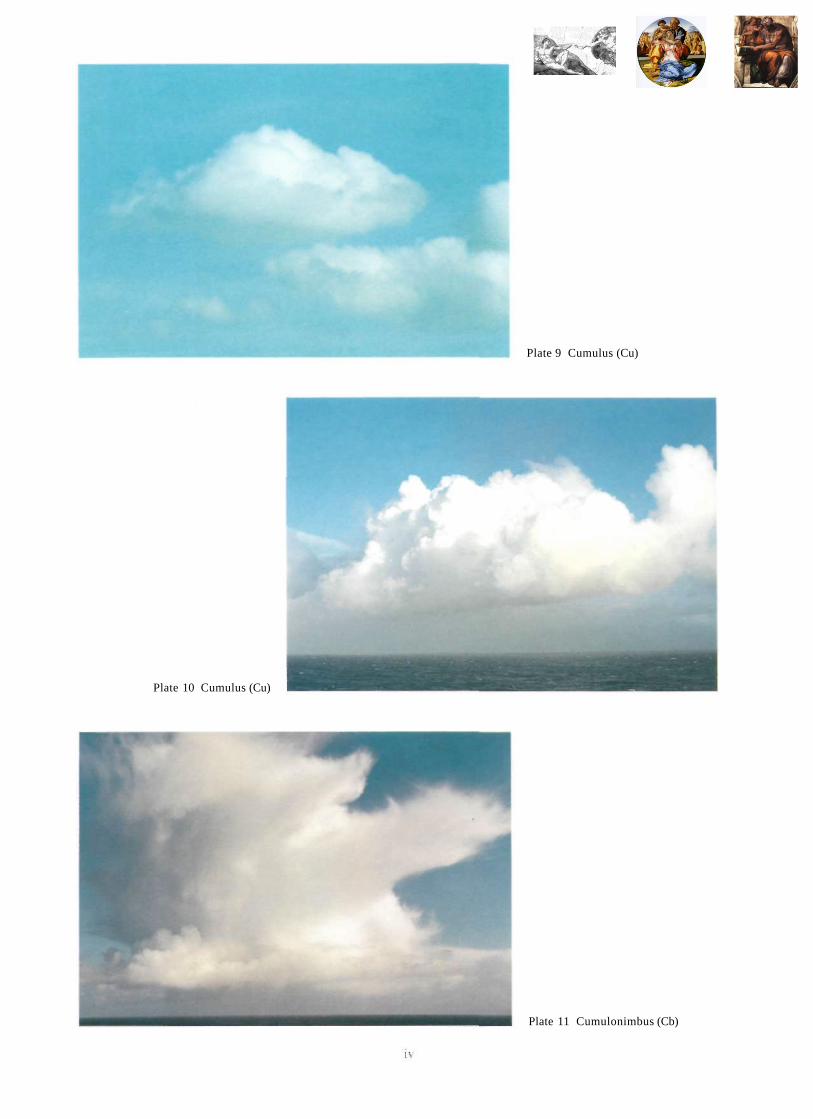
Plate 9 Cumulus (Cu)
Plate 10 Cumulus (Cu)
Plate 11 Cumulonimbus (Cb)

Plate 14 Cumulonimbus-developing from cumulus (12), after ten minutes (13) and after forty minutes (14)
Plate 13 Cumulonimbus developing from cumulus (12), after ten minutes (13) and after forty minutes (14)
Plate 12 Cumulonimbus — developing from cumulus (12), after ten minutes (13) and after forty minutes (14)

Plate 15 Cumulus (Cu) and Stratocumulus (Sc)
Plate 16 Waterspout
Plate 17 Orographic Cloud
vi

Plate 18 Lenticular Cloud
Plate 19 Cumulonimbus precipitating
Plate 20 Lightning
Vl l

Plate 21 Entering sea fog in the English Channel haze but no fog
Plate 22 Entering sea fog in the English Channel fog developing
Plate 23 Entering sea fog in the English Channel—fog
viii

Plate 24 Arctic Sea Smoke St Lawrence Seaway
Plate 25 Pampero
ix
Plate 24 Arctic Sea Smoke St Lawrence Seaway
Plate 25 Pampero

Plate 28 Rainbows primary and secondary
Plate 27 Trade Wind cumulus
Plate 26 Effect of a temperature inversion—North Sea

Plate 29.1 Contrails
Plate 29.2 Contrails
XI

Plate 30 Force 0
Plate 31 Force 1
Plate 32 Force 2
M l

Plate 33 Force 3
Plate 34 Force 4
Plate 35 Force 5
xiii

Plate 36 Force 6
Plate 37 Force 7
Plate 38 Force 8
XIV

Plate 39 Force 9
Plate 40 Force 10
Plate 41 Force 11
xv

Plate 44 Extreme storm wave, North Atlantic, Force 12
xvi
Plate 43 Swell and wind waves Force 2-3
Plate 42 Force 12

TEMPERATE AND POLAR ZONE CIRCULATION 63
SECONDARY DEPRESSIONS
A secondary depression is one which develops and is embedded within the circulation of a larger depression termed the primary depression. The secondary depression moves in the direction of the general air flow around the primary; this movement is termed cyclonic. Thus it will move anticlockwise in the northern hemisphere and clockwise in the southern hemisphere. The central pressure value of the secondary depression is initially greater than that of the primary. However, as the primary has begun to decay when the secondary begins to develop, the latter will eventually have the lower pressure value. Finally the secondary takes over the circulation of the primary and one area of low pressure will then exist.
While secondary depressions may be frontal or non-frontal, the most common type are frontal which develop on the trailing cold fronts of primary depressions (Fig. 8.14(1)). Frontal secondary depressions have life cycles similar to that of any frontal depression and will be a member of a family of depressions, but all members of the family are not necessarily secondary depressions (compare Figs. 8.6 and 8.14( 1)).
Non-frontal secondary depressions normally develop in the unstable air stream to the rear of an occluding depression. The form of the isobars associated with the feature is markedly circular (Fig. 8.14(2)). Cumuliform cloud and precipitation occur in its central area, and extend along the trough line on the side of the secondary furthest displaced from the primary depression. An area of slack pressure gradient with associated light variable winds exists between the two areas of low pressure. However, on the side of the secondary, furthest from the primary, there is an area of steep pressure gradient and high wind speeds.
ANTICYCLONES
The simplified general circulation implies the existence of high pressure areas in the subtropical and polar regions (Fig. 8.1). In the actual circulation these areas of high pressure take the form of anticyclones and are represented on surface charts by a set of closed isobars of oval or sometimes circular form (Figs. 8.3, 8.11). In contrast with frontal depressions, anticyclones move slowly eastwards, or may be stationary (Fig. 8.6).
In the sub-tropics, anticyclones persist for long periods and are termed permanent. Those in the North Atlantic are called the Bermuda and Azores anticyclones, reflecting their preferred location, and in the North Pacific there is a similar pattern of two anticyclones. However, in the southern hemisphere subtropical anticyclones move eastwards at greater speeds than those of the nothern hemisphere.
The term semi-permanent is applied to the anticyclonic conditions which develop seasonally in temperate and polar zones. Examples are anticyclones which develop over North America and Siberia in winter, but it should be noted that these areas are also frequently affected by frontal depressions.
Anticyclones may be either warm or cold. Warm anticyclones (all subtropical and some higher latitude anticyclones) are typified by a mainly warm troposphere. A cold anticyclone is one in which the lower troposphere is occupied by cold air, thus it has a relatively shallow circulation (e.g. anticyclones which move rapidly into lower latitudes behind a family of depressions). Some anticyclones show both cold and warm attributes, with a shallow layer of cold air at and near the surface, and warm air in the troposphere above. These exist in temperate zones during the winter months, when slow moving or stationary warm anticyclones persist over a large land mass. The radiative cooling of the surface results in the development of a layer of cold air in the lower troposphere.
As the pressure gradient is slack, the central area of an anticyclone is either calm or has light and variable winds. Towards the outskirts of the system wind speed increases and wind direction becomes more marked, being outwards and clockwise in the northern, but anticlockwise in the southern hemisphere. The air flow is divergent at the surface, but convergent in the upper part of the troposphere with a subsequent downward movement of air in the troposphere, termed subsidence (Fig. 8.15(1)). In the early stages of the development of an anticyclone the rate of subsidence is high but decreases as the system develops. Subsidence is significant in modifying the environmental lapse rate as the air warms adiabatically. If the process continues over a period, an upper level temperature inversion develops.

promoting a stable atmosphere at this level (Fig. 8. 15(2)). The height at which the inversion is present varies within an anticyclone, and from one anticyclone to another, depending upon the degree of subsidence.
In the early stages of anticyclonic development, cloud in the upper and middle troposphere will clear as a result of subsidence, hence the clear skies associated with most anticyclones. Subsequently subsidence and adiabatic warming result in low relative humidity values, which are particularly noticeable at the level of the inversion.
Weather Conditions
In an anticyclone, the environmental lapse rate of the lower troposphere is variable, as it is affected by the diurnal variation of surface temperature. Such variations are most significant over land, and play an important part in determining anticyclonic weather conditions.
In summer months, a warm anticyclone over land results in high air temperatures during the day. Any cloud developing will be fair weather cumulus, its vertical extent being limited by the upper level

TEMPERATE AND POLAR ZONE CIRCULATION 65
inversion. Its life span will be short as the relative humidity of the surrounding air is low. Visibility on land may well be reduced as a result of haze, and in coastal areas sea breezes develop. Overnight clear skies and low wind speeds favour the formation of dew, a deposit of water droplets on the surface. Dew forms as a result of air, in contact with the surface, being cooled below its dew-point temperature. Radiation mist or fog may develop locally where there is a high relative humidity and downslope drainage of cold air. Soon after sunrise the mist or fog disperses.
During winter, the weather conditions initially are clear skies and low air temperatures during the day, while overnight air temperatures often decrease below freezing point. Condensation occurs if the air is cooled below its dew-point temperature. Water droplets forming on the surface may freeze and further cooling of the air results in sublimation and the development of a white crystalline deposit termed hoar frost. Alternatively, a high relative humidity and a long cooling period may cause widespread and rapid formation of radiation fog, which drifts offshore over coastal waters and estuaries. The fog may persist throughout the following day as a result of the small amount of solar radiation reaching the surface due to the time of year and the presence of the fog {Chapter 6). However, during the day the fog may lift over land to form a cover of low level stratiform cloud, which in the late afternoon appears to "lower" to the surface, the condition being termed anticyclonic gloom. If the air temperature is below 0°C, the fog droplets will be supercooled and will freeze on coming into contact with any object whose temperature is at or below 0°C. The white deposit of ice is called rime and always accumulates on the windward side of the object.
When smoke and other pollutants are trapped beneath the upper level inversion of an anticyclone because of the stable atmospheric conditions at this level, smog exists (Plate 26). This term is derived from smoke and fog, but is also used to describe conditions produced by pollutants without fog (e.g. in Los Angeles).
Anticyclonic weather conditions in summer and winter may persist for an extended period, and a change in conditions depends on the movement or general weakening of the anticyclone. The change is indicated by increasing wind speeds caused by steepening pressure gradients, normally associated with an advancing depression.
RIDGES OF HIGH PRESSURE
An extension of an anticyclone identified by the form of isobars on a surface pressure chart is termed a ridge (Fig. 8.3), the point of maximum curvature of the isobars denoting its axis. A ridge may often be a direct extension of a large anticyclone and produces typical anticyclonic weather while it persists. In contrast, a ridge located between two frontal depressions moves rapidly over an area, resulting in a short-lived break in the adverse weather of the depressions. If the axis of the ridge is approached from the east, decreasing wind speeds are experienced as the pressure gradient slackens. Cloud cover decreases, possibly giving clear skies, or cumuliform cloud without precipitation. To the west of the axis, wind speeds increase as the pressure gradient steepens. Cloud cover which increases and progresses from cirrus (Ci) to cirrostratus (Cs) indicates an advancing frontal depression.
COLS
If there are two anticyclones and two depressions arranged alternately, a feature exists between them termed a col (Fig. 8.3). Within the col the pressure gradient is slack, and the winds light and variable. Other weather conditions associated with a col will depend upon the effect of the underlying surface on the air mass above. Thunderstorms are probable if there is instability, but with stability radiation fog may develop, or advection fog where warm air passes over a colder surface. During winter, cols are relatively short-lived due to the rapid movement of depressions which surround them.

66 METEOROLOGY FOR SEAFARERS
AIR MASSES
An air mass is a large body of air whose temperature and relative humidity values are more or less uniform in a given horizontal plane. Its horizontal dimensions are of the order of hundreds or even thousands of square kilometres. The most suitable conditions for the development of an air mass are a combination of a uniform part of the earth's surface and the presence of a large anticyclone for at least three days. The slack surface pressure gradient, and hence low wind speeds, of the anticyclone enables the air mass to acquire its properties. Thus the source regions of air masses are generally found in the subtropical, temperate and polar zones, where uniform surfaces and anticyclonic conditions exist simultaneously. Air masses are therefore classified as Tropical, Polar or Arctic (Antarctic), to indicate their source regions and their relative temperatures. Arctic (Antarctic) air masses originate within the Arctic (Antarctic) circles, and are colder than the Polar air mass which originates to the south (north) of this region. Air masses are further sub-divided into maritime (high humidity), or continental (low humidity) as in the following table:
Table 8.4 Characteristics of air masses
Modification of Air Masses
Once an air mass leaves its source region, it will no longer be in equilibrium with the underlying surface which may be either warmer or colder than the air mass. The mass will be heated or cooled, and both its temperature and environmental lapse rate will change. If it is heated by the surface, the E.L.R. increases and it becomes unstable, whereas if it is cooled by the surface the E.L.R. decreases, and it becomes stable (Chapter 3). The relative humidity of the mass is also affected by changes in temperature, increasing when the mass is cooled, and decreasing when the mass is heated. However, when the mass is heated, evaporation from the surface occurs, counteracting the effect of heating on the relative humidity value. Therefore in establishing the final RH value of the air mass, both heating and evaporation effects must be taken into account.
Other processes in the atmosphere, for example convergence, which are not further considered, may also modify the characteristics of an air mass.
Weather Conditions
To illustrate the conditions associated with an air mass the weather experienced over the British Isles is taken as an example. This choice of example is not as restrictive as might first appear, since the conditions generated by an air mass are similar to those experienced in other parts of the world. Typical synoptic patterns associated with the five principal air masses affecting the British Isles are shown in Fig.

TEMPERATE AND POLAR ZONE CIRCULATION 67
8.16. The nature of the surface over which each air mass passes before arrival over the British Isles is identifiable, thus changes in the characteristics of each air mass and the related weather conditions can be assessed.
Tropical maritime (Tm) affects the British Isles both in winter and summer. It moves from the Azores northwards over progressively cooler surfaces and, having been subjected to cooling, its relative humidity increases and it becomes stable. Advection fog may occur, particularly in spring and early summer, in the Western Approaches and English Channel. In the summer low level stratus may develop over the sea and also affect windward coasts. Inland, cloud amount is less, while on the east coasts clear skies are probable, reflecting the heating of the air mass as it passes over the warmer land surface.
During the winter months, advection fog is more probable over land, particularly if the surface has been subjected to a period of low temperatures. Dependent upon the wind speed, low level stratus with drizzle is possible over land or sea. Orographic cloud with rain may develop over high ground. Air temperatures are above the seasonal average.
Tropical continental (Tc) is uncommon, and is only experienced over the British Isles in the summer months. From its source region in the Sahara desert it passes over the Mediterranean and Europe. Although cooled slightly, it produces high air temperatures well above the seasonal average. During the day unstable conditions and convection currents develop. However, in spite of its sea passage the relative humidity of the air mass is low, thus there is a general lack of cloud, and the air temperature is enhanced. Haze may develop.
(1) Tropical maritime (Tm) (2) Tropical continental (Tc)
Fig. 8.16 Air masses typical surface synoptic chart.

68 METEOROLOGY FOR SEAFARERS
Polar continental (Pc) originates in Northern and Western Europe and Russia. During the winter, the North Sea is warmer than the air mass and instability develops as the air is heated, its relative humidity simultaneously increasing. Convection over the sea may result in cumulus and cumulonimbus clouds, but, if the sea passage is short, only stratocumulus may develop. The eastern seaboard is affected by cloud with showers of snow, hail or sleet. Western areas experience generally clear sky conditions which favour the development of hoar frost, or possibly radiation fog overnight if wind speeds are low enough. Below seasonal average temperatures are experienced in spite of the heating of the air mass.
In summer the Polar continental air mass is cooled by the North Sea and becomes more stable. Advection fog or low level stratus forming over the sea affects the east coast, where the air temperatures are generally below the seasonal average. In contrast, areas a short distance inland and to the west experience clear skies with higher air temperatures, and haze may develop during the afternoon.
Polar maritime (Pm) is an air mass frequently affecting the British Isles. Approaching from the west and north-west, its maritime properties of high relative humidity and unstable conditions develop during its long transit over the North Atlantic. Convection over the sea results in cumulus and cumulonimbus clouds, which in winter on the western side of the country are accompanied by showers of rain, sleet or snow or sometimes hail. Eastern areas experience little or no cloud cover, thus favouring the development of hoar frost or radiation fog during the night. Air temperatures are generally the seasonal average. In summer convection occurs over sea and land, and cloud cover is widespread with associated showers of rain, hail, and possibly thunderstorms. The air mass is cool with air temperatures below the seasonal average.
(3) Polar continental (Pc) (4) Polar maritime (Pm)
Fig. 8.16 Air masses—typical surface synoptic chart.

TEMPERATE AND POLAR ZONE CIRCULATION 69
(5) Arctic maritime (Am)
Fig. 8.16 Air masses typical surface synoptic chart.
Arctic (A) is an air mass originating in the Arctic Basin, and is normally experienced only in winter and spring. On its passage to the British Isles, maritime properties develop and it becomes Arctic Maritime (Am). Its relative humidity increases, and a steep lapse rate develops as it is heated by the warmer sea. Showers of snow and hail are usually experienced in Scotland and on the windward coasts of the North Sea. Skies are clear inland, and air temperatures are below the seasonal average.

CHAPTER 9
TROPICAL AND SUBTROPICAL CIRCULATION
INTRODUCTION
This chapter considers the circulation of the atmosphere in the tropical zone from the Equator to 23° 27'N and S, and the subtropical zones from 23° 27'N and S to approximately 40°N and S. Surface synoptic charts of these zones show significant differences compared with those of temperate zones, the
Fig. 9.1 Tropical and subtropical circulation typical surface synoptic chart.
pressure distribution appearing generally less complex with slacker pressure gradients (Fig. 9.1). In addition to subtropical anticyclones (Chapter 8), tropical cyclones, the Intertropical Convergence Zone, Equatorial Trough, Doldrums, Trade Winds and monsoons are features of the atmospheric circulation of these zones.
70


72 METEOROLOGY FOR SEAFARERS
number per annum varying from one area to another (Table 9.1 and Fig. 9.3). However, it should be noted that there has been a paucity of data in the past for certain areas, and recent observations suggest that the freauency of tropical cyclones may be greater, particularly in the southern hemisphere.


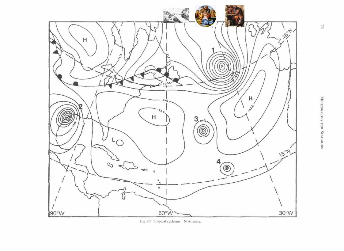

TROPICAL AND SUBTROPICAL CIRCULATION 77
Formation
The more frequent formation of tropical cyclones during summer and autumn in particular areas suggests that certain conditions are necessary. Research has shown that a sea surface temperature of at least 27°C is required. At this temperature saturated air has a large water vapour content (Fig. 4.2—T), and as the air ascends, adiabatic cooling causes condensation. The latent heat of vaporisation released is an important source of energy for the development and continued maintenance of a tropical cyclone. The significance of the sea surface temperature is also illustrated by the point of origin of a cyclone tending to move into higher latitudes, and subsequently into lower latitudes as the season progresses. The tracks of tropical cyclones (Fig. 9.3) show that their formation occurs at least 5°N or S of the Equator, which suggest that the value of the Coriolis force is critical. The evolution of a tropical cyclone from a tropical depression in which cumuliform cloud is developing, is only possible in an atmosphere where the vertical wind shear has a small value. Thus the area where a tropical cyclone is likely to develop must not be under the direct influence of a jet stream.
The development of an existing tropical depression into a tropical cyclone depends upon the amount of water vapour entering the system, the latent heat of vaporisation released resulting in the development of a warm core. The eye of the system first appears in the upper part of the troposphere and then descends. As the air in the eye descends (Fig. 9.4), it warms adiabatically, enhancing the development of the warm core. These factors contribute to the decrease in surface pressure with the attendant steepening pressure gradient as the system develops, thus further energy enters the system. Of the total energy of the system, a small amount is converted into kinetic energy, but a far larger amount is exported through its upper level circulation associated with the Cb anvils. If favourable atmospheric and sea surface conditions persist, the system continues to evolve, its associated wind speeds increase, and it becomes a tropical cyclone.
Decay
During its evolution the tropical cyclone may move onshore, and, as the energy derived from water vapour is reduced, the tropical cyclone may decay rapidly. If it subsequently moves offshore it may well be revitalised. Whether the cyclone moves out to sea or remains offshore throughout its existence, it eventually moves into higher latitudes where, with the gradual reduction in surface temperature, its intensity decreases. In higher latitudes the warm air of the system may become part of the warm sector of a frontal depression.
Movement
The initial track of a tropical cyclone in lower latitudes is generally from east to west as it is steered by the easterly tropospheric air flow in which it is embedded. As a pole-ward component is also present, its track may be close to WNW in the northern hemisphere and WSW in the southern hemisphere, along the equatorward margin of the subtropical anticyclone. During this stage the system moves at about 10 knots. A tropical cyclone recurves between 20° and 30°N or S when it reaches the western edge of the anticyclone. Its track is then north (N Hemisphere) or south (S Hemisphere), its speed of advance decreases, and it may become stationary for a period. It then tracks north-easterly (N Hemisphere), and speed of advance increases to 20 knots or greater. The system has now left the tropical circulation and is being steered by the general westerly tropospheric airflow of the mid-latitudes (Fig. 9.3).
On occasions a tropical cyclone may not recurve but follows the alternative path (Fig. 9.6). In most cases this is directly related to the position and movement of the subtropical anticyclone which blocks the path of recurvature. At a later stage, however, the system may recurve unless it moves onshore and decays rapidly.
Variations occur, and no two tropical cyclones have exactly the same track. In Fig. 9.7 the track of 2 was influenced by the subtropical anticyclone and did not recurve, but made landfall in the Gulf of Mexico, while 1 recurved along the eastern seaboard of North America; 3 is recurving, and 4 may follow 3.

78 METEOROLOGY FOR SEAFARERS
Weather and Sea State
Weather and sea state conditions associated with tropical cyclones are extreme, and the loss of life and financial costs arising from the damage caused can be high. Fig. 9.8 shows probable wind conditions likely to be encountered. The sea state is directly related to these conditions, but within the eye the seas are confused due to the high winds which recently prevailed. Extreme storm waves generated by the wind may be amplified by astronomical tides, and thus become storm surges which cause extensive damage in coastal areas. Showers, light on the periphery of a cyclone, increase in frequency and intensity to reach a maximum on the outskirts of the eye itself. Within the eye, low level stratiform cloud may occur over the sea and clear skies over land.
Ship Action
Bulletins issued by meteorological services detail not only tropical cyclones but also the preceding stages of tropical depressions and storms. The seafarer must collect, analyse and update this data in order to determine the best course to follow. In addition to this forward assessment, the present conditions of weather and sea state should be observed, as these provide a cross-check on the meteorological bulletins.
Before bulletins became available, a procedure called the Single Observer's Action was developed as a result of seafarers' experiences, and this procedure, which is still relevant, covers the following:
Warning signs of the presence of a tropical cyclone Procedure to establish the location of the vessel in a tropical cyclone. Evasive action to be taken by a vessel.
Warning Signs
Swell. Depending upon the extent of open ocean, an early indication of a tropical cyclone is the swell generated by the winds within the system. These swells, whose general characteristics are long wavelengths and low wave height, have been observed at some 600 n. mile from the centre. The direction from which the swell comes is an indication of the bearing of the centre of the cyclone when the swell was generated. Skies. An unusually clear day may precede the appearance of cirrus cloud with brightly coloured sunsets and sunrises. The cloud base subsequently lowers, with the onset of showers in the outer regions of the system.
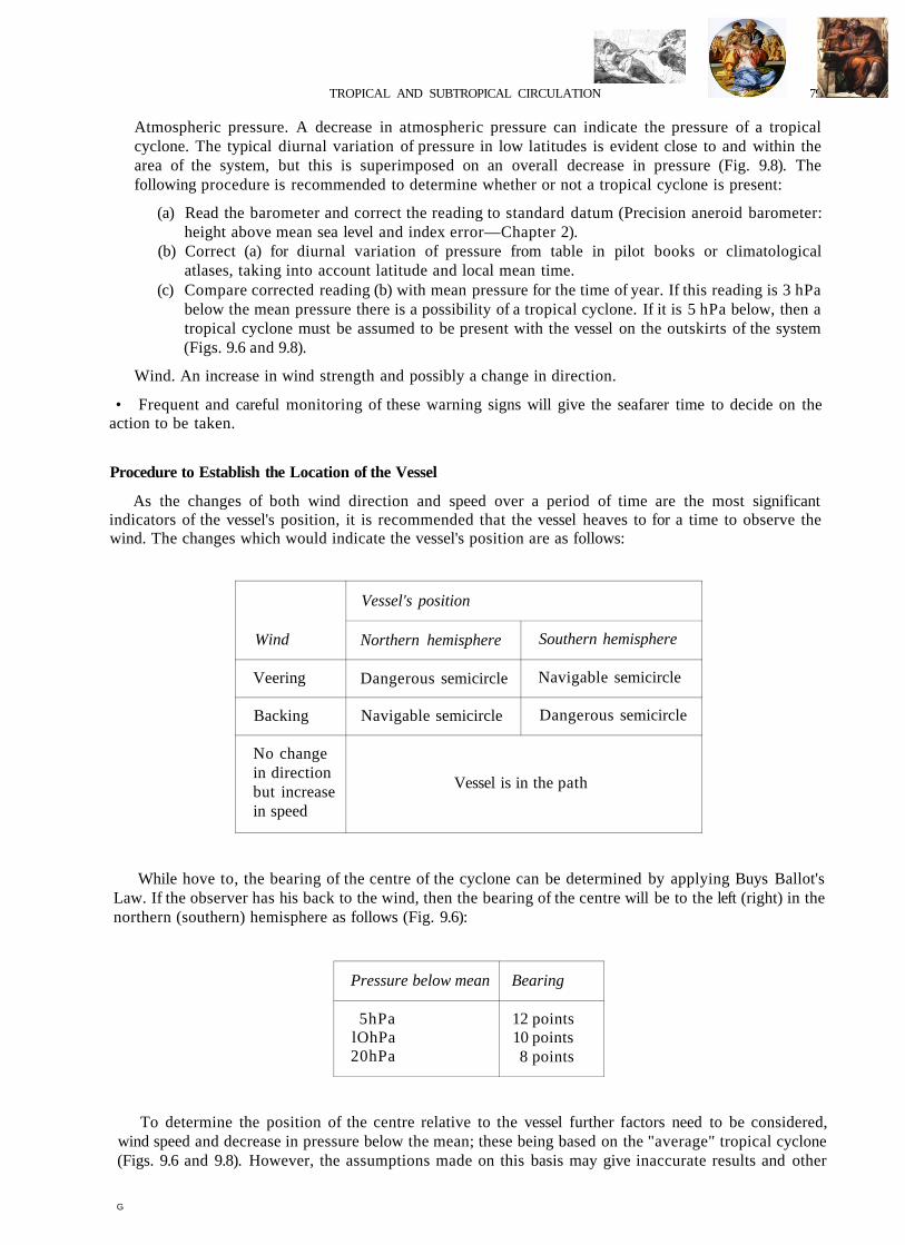
TROPICAL AND SUBTROPICAL CIRCULATION 79
Atmospheric pressure. A decrease in atmospheric pressure can indicate the pressure of a tropical cyclone. The typical diurnal variation of pressure in low latitudes is evident close to and within the area of the system, but this is superimposed on an overall decrease in pressure (Fig. 9.8). The following procedure is recommended to determine whether or not a tropical cyclone is present:
(a) Read the barometer and correct the reading to standard datum (Precision aneroid barometer: height above mean sea level and index error—Chapter 2).
(b) Correct (a) for diurnal variation of pressure from table in pilot books or climatological atlases, taking into account latitude and local mean time.
(c) Compare corrected reading (b) with mean pressure for the time of year. If this reading is 3 hPa below the mean pressure there is a possibility of a tropical cyclone. If it is 5 hPa below, then a tropical cyclone must be assumed to be present with the vessel on the outskirts of the system (Figs. 9.6 and 9.8).
Wind. An increase in wind strength and possibly a change in direction.
• Frequent and careful monitoring of these warning signs will give the seafarer time to decide on the action to be taken.
Procedure to Establish the Location of the Vessel
As the changes of both wind direction and speed over a period of time are the most significant indicators of the vessel's position, it is recommended that the vessel heaves to for a time to observe the wind. The changes which would indicate the vessel's position are as follows:
Wind
Veering
Backing
No change in direction but increase in speed
Vessel's position
Northern hemisphere
Dangerous semicircle
Navigable semicircle
Southern hemisphere
Navigable semicircle
Dangerous semicircle
Vessel is in the path
While hove to, the bearing of the centre of the cyclone can be determined by applying Buys Ballot's Law. If the observer has his back to the wind, then the bearing of the centre will be to the left (right) in the northern (southern) hemisphere as follows (Fig. 9.6):
Pressure below mean
5hPa lOhPa 20hPa
Bearing
12 points 10 points 8 points
To determine the position of the centre relative to the vessel further factors need to be considered, wind speed and decrease in pressure below the mean; these being based on the "average" tropical cyclone (Figs. 9.6 and 9.8). However, the assumptions made on this basis may give inaccurate results and other
G

80 METEOROLOGY FOR SEAFARERS
data sources should be consulted. The approximate track can be established from two or more bearings of the centre, with an interval of two or three hours between each observation.
Evasive Action
Once the vessel's position in the tropical cyclone is established, evasive action, as indicated in Tables 9.3 and 9.4 and using best speed, can be taken. This action increases the distance between the vessel and the centre of the cyclone as rapidly as possible.
Table 9.3 Evasive action by vessel in N Hemisphere (Fig. 9.9)
Semicircle
Dangerous
Navigable or path of storm
Action
Place wind1-4 points on starboard bow altering course to starboard as the wind veers.
Place wind on starboard quarter altering course to port as wind backs.
Fig. 9.9
1
2
PATH
TRACK
Fig. 9.9 Evasive action N Hemisphere.
Table 9.4 Evasive action by vessel in S Hemisphere (Fig. 9.10)
Semicircle
Dangerous
Navigable or path of storm
Action
Place wind 1 -4 points on port bow altering course to port as wind backs.
Place wind on port quarter altering course to starboard as wind veers.
Fig. 9.10
1
2

TROPICAL AND SUBTROPICAL CIRCULATION / 81
Fig. 9.10 Evasive action S Hemisphere.
While evasive action is being taken, the seafarer must continue to monitor the conditions. These will indicate when the vessel is clear of the cyclone and the original course and speed can be resumed. In latitudes where recurvature is possible, monitoring is particularly important, since the initial evasive action, taken by a vessel in the dangerous semicircle and maintained while the cyclone recurves, may result in the vessel re-entering the system and possibly the eye.
Where insufficient sea room prevents the evasive action recommended, a vessel in the dangerous semicircle should if possible heave to with the wind on the starboard (port) bow in the northern (southern) hemisphere, thus heading away from the centre. In the navigable semicircle in either hemisphere, the vessel should heave to in the most comfortable position relative to wind and sea conditions.
The regulations in the International Convention for the Safety of Life at Sea 1974 (SOLAS 1974) recommend that vessels encountering a tropical cyclone should inform the nearest coastal radio station and all other vessels in the vicinity of its existence, and should update the information at least every three hours while it is affected by the system.
Appendix I is an extract of an account of a particular tropical cyclone reproduced by permission of Mr J. W. Nickerson and the Mariners Weather Log Vol. 27 No. 1. The additional comments were published in Seaways, May 1984.
INTERTROPICAL CONVERGENCE ZONE
The Intertropical Convergence Zone (ITCZ) is the area in low latitudes in which the trade winds of the two hemispheres converge. In this zone the horizontal convergence and subsequent ascent of air in the troposphere results in cloud development. Analysis of satellite images (Fig. 9.5) show that, while cloud development is a feature of this zone, it is not continuous in the horizontal plane at any given time, nor is it a persistent feature at any particular point over a period. The cloud type is cumuliform, ranging from cumulus to cumulonimbus, with diameters between 1 and 10 km. A collection of these clouds, termed a convective cell, may have a diameter in the range of 10 and 100 km. A number of such cells may form a cloud cluster which may have a diameter in the range of 100 km and 1000 km. Weather conditions may be

Fig. 9.11 Streamline chart for the N Pacific.
light winds, squalls and showers (Cu cloud), or thunderstorms and heavy precipitation (Cb cloud). In contrast clear skies indicate that there is no convergence of air with its resultant ascent.
The intermittent nature of convergence, both in time and space, has resulted in the use of an alternative term Intertropical Confluence. Confluence implies the nearer approach of adjacent streamlines in the direction of air flow; a streamline being a curve plotted parallel to the instantaneous direction of the wind vector (Fig. 9.11). The technique of streamline analysis is of great value in tropical meteorology since areas of surface convergence can be defined. The convergent flow may be that associated with a tropical depression which, under suitable conditions, may later develop into a tropical cyclone. Fig. 9.11 illustrates two fully developed tropical cyclones and one tropical storm.
The position of the ITCZ varies throughout the year (Fig. 9.12), progressing north between January and July, and south in the latter half of the year. The range of latitude covered varies from one longitude to another, being greatest in the Indian Ocean, and least on the eastern side of the North Atlantic and North Pacific Oceans, where it does not move south of the Equator. In the South Atlantic its progress south of the Equator is minimal, a factor which may partially account for the lack of tropical cyclones in this ocean (Fig. 9.3).
In certain ocean areas the ITCZ may be a single band (Fig. 9.12), or it may be a more complex double band feature.


84

TROPICAL AND SUBTROPICAL CIRCULATION 85
TRADE WINDS
Trade Winds are defined as the winds which exist between the subtropical anticyclone and the ITCZ. The North-East Trades are in the northern hemisphere and the South-East Trades in the southern hemisphere. The term derives from their reputation for constant direction and speed, which made them reliable for sailing vessels. The general extent of trade winds, as shown by the vector mean winds, the mean position of the ITCZ, and mean pressure value of the subtropical areas are illustrated for January in Fig. 9.15 and for July in Fig. 9.16. It should be noted that, in the North Indian Ocean in July, the typical North-East Trades evident in other areas are absent, and the particular feature of the area is the Monsoon (see below).
The wind direction within each trade wind zone varies, and steadiness of direction and speed is a marked feature only in the core of the zone in each ocean. The average strength is Force 4, which can vary in the short term. There is a general tendency for an increase in strength during the winter season in each hemisphere.
The cloud is the trade wind cumulus which occurs as cloud streets, with an average cover of four-eighths (Plate 27). An important cloud characteristic is its greater vertical development and associated showers nearer the equator and western side of the oceans, reflecting the height at which the trade wind inversion exists in the troposphere. On occasions, the trade winds may be absent, their place being taken by other systems (e.g. tropical depressions or tropical cyclones).
MONSOONS
Monsoon, derived from the Arabic "mausim" meaning season, was the name originally given to the winds in the Arabian Sea which reversed in direction from one season to another. It is now used to define that part of the atmospheric circulation covering a large geographical area over which a clearly predominant wind direction prevails in one season, with a reversal or near reversal of wind direction in the following season. This phenomenon occurs over the North Indian Ocean and most of the Southern Asian continent where the North-East Monsoon prevails in the winter months (Fig. 9.17), and the South-West Monsoon in the summer months (Fig. 9.18). The regional features of the Tibetan Plateau and the Himalayas play a significant part in their generation.
In the North Indian Ocean the monsoon periods are as follows:
North-East Monsoon—November to March Intermonsoon period—April and May
South-West Monsoon—June to September Intermonsoon period—October
North-East Monsoon
The mean pressure chart for January (Fig. 9.15(2)) shows an extensive area of high pressure over the Asian continent, with decreasing pressure south towards the Equator. The vector mean wind chart (Fig. 9.15(1)) for the same month shows north-easterly winds across the Arabian Sea and the Bay of Bengal. The typical surface synoptic chart for a day in January shows in greater detail the actual surface pressure distribution (Fig. 9.17), and confirms the north-easterly winds. At the height of the season the winds are Force 3 to 4 in the area, except near the Equator where Force 2 to 3 is normal. Generally, cloud cover is minimal with little or no rain. In December and January there is more cloud and rain in the southern area of the Bay of Bengal. The monsoon may be interrupted in the Arabian Sea, north of 20°N, with wind direction changing and speed increasing when a frontal depression passes eastwards across the Asian continent.
South-West Monsoon
The mean pressure chart for July (Fig. 9.16(2)) shows an extensive area of low pressure centred over


TROPICAL AND SUBTROPICAL CIRCULATION 87
North-West India, with increasing pressure values towards the equator. The vector mean wind chart (Fig. 9.16(1)) for the same month shows south-west winds over the North Indian Ocean which correspond to this pressure distribution. The typical surface synoptic chart for a day in July (Fig. 9.18) confirms this distribution. In addition to the area of low pressure over North-West India, which can be termed a thermal low, other depressions may be present which result in rain over the Indian subcontinent and surrounding areas.
At the height of the monsoon, winds over the Arabian Sea achieve Force 6, with Force 7 or greater being possible on more than ten days a month. To the east of Socotra such conditions occur for 50% or more of the time in July. In the Bay of Bengal winds average Force 4 to 5, with Force 7 or greater occurring between 5 and 10 days a month in July and August. In the area between 5°N and the Equator and east of 60°E winds are generally Force 3, their direction being between south and west.
Along the west coast of India, clouds and rain may occur as a result of the orographic effects of the Western Ghats. In the northern part of the Arabian Sea, extensive cloud and precipitation can occur for several days due to the presence of a depression termed a subtropical cyclone. Generally visibility is moderate in the northern and western parts of the Arabian Sea, but poor near the coast as a result of either precipitation or dust haze. At the head of the Bay of Bengal, and in the Ganges Delta, there may be precipitation associated with depressions termed monsoon depressions which subsequently move westwards across India.
Intermonsoon Periods
The two intermonsoon periods of April and May, and October, are relatively short with the progressive shift of the Equatorial Trough northwards and southwards respectively. Conditions in the trough vary greatly, ranging from calm or light winds and generally fair or fine, to squalls and cumuliform cloud with heavy rain and thunderstorms. During the months of May, June, October and November, the sea surface temperature in the Arabian Sea reaches the critical value of 27°C, and upper tropospheric conditions are more favourable for the development of tropical cyclones. In the Bay of Bengal the cyclone season normally achieves its peak in October and November, with storm surges and heavy rainfall in the Bay and along adjacent coasts.
Along the western coastline of India, onshore winds may occur during April and May. These are local sea breezes developing in response to the rapid increase of land surface temperature compared with that of the sea. West of55°E and within 5° to 10° of the Equator in the Arabian Sea, south-westerly winds occur during this period, whose strengths increase to Force 7 at times. These conditions reflect the early stages in the development of the cross-equatorial air flow from the southern to the northern hemisphere. The range of latitude, over which this flow occurs, increases progressively to a maximum at the height of the South-West Monsoon (Fig. 9.15, 9.18). The cross-equatorial flow is concentrated in the lower troposphere and is not uniform over a range of longitude, being significant over a span of 15° west of 55DE. Within this flow there is a change of wind direction from south-east to south-west as it moves from the southern into the northern hemisphere.
North Pacific Monsoons
The annual conditions occurring in the North Indian Ocean are also experienced further east in the China and Yellow Seas, and in the western extremities of the North Pacific south of 30°N.
The North-East Monsoon first becomes evident in the northerly part of the area in September, eventually affecting the entire area north of the Equator by November. Although referred to as the North-East Monsoon, the wind direction varies, particularly with increasing latitude. Wind strength is generally Force 6 in the Taiwan Straits and Force 5 in the China Sea, except in the area south of 10°N where Force 4 is common. Near the Equator winds are northerly and light. North of 18°N, periods of overcast skies with light rain or drizzle alternating with broken cloud cover occur between January and April. South of 18°N over the open sea, cloud cover is generally four-eighths increasing towards the Equator with an increasing frequency of showers. Cloud and precipitation amounts are greater where the wind blows onshore over high ground. These conditions persist until April when the prevailing wind direction becomes less steady and winds with a southerly component occur more frequently. This change marks the beginning of the South-West Monsoon which reaches its peak in July (Fig. 9.16).

88 METEOROLOGY FOR SEAFARERS
At the height of the South-West Monsoon, wind direction varies between south-east and south-west in the area lying west of 140°E and south of 40°N. The core of the monsoon is in the South China Sea where winds of Force 3 to 4 occur; elsewhere winds average Force 3. In general the winds are lighter during the South-West Monsoon, the reverse of the conditions experienced in the North Indian Ocean. Cloud cover averages four-eighths with occasional showers, except in windward coastal areas where it is greater and the rainfall heavier.
MONSOON TYPE WEATHER
In certain other low latitude areas there are seasonal changes in wind direction accompanied by a change in the amount of rainfall. Such areas do not strictly speaking have monsoons, but monsoon-type weather.
Gulf of Guinea
During summer, the Gulf of Guinea and mainland Africa to the immediate north, experience south-west winds with cloud development and precipitation (Fig. 9.16). This is termed the South-West Monsoon. Both at the beginning and end of the South-West Monsoon, violent thunderstorms with severe squalls moving from east to west and of fairly short duration may occur near the coast. Locally these are known as Tornadoes.
During the remainder of the year the area has a dry season, with the wind in the Gulf of Guinea being between south and west, and the remaining area experiencing winds generally between north and east. Between November and February an easterly wind, called the Harmattan, with a low relative humidity value transports dust and sand from the Sahara Desert. The dust and sand may be carried several hundred miles offshore generating poor visibility. At other times visibility is moderate as a result of haze.
Northern Australia
Between November and March, the North-West Monsoon prevails along the northern coastline of Australia and the adjacent seas, with wind direction between west and north. The flow of air is cross-equatorial from the northern hemisphere (Fig. 9.15), the winds seldom achieving Force 7, with cloudy conditions and heavy rain showers. During the summer the South-East Trades prevail over the area (Fig. 9.16).

CHAPTER 10
ORGANIZATION AND OPERATION OF METEOROLOGICAL SERVICES
INTRODUCTION
A forecast is a statement of the anticipated meteorological conditions for either an area, or fixed location, or along a route or routes for a specified period. The term was introduced by Admiral Fitzroy, the first head of the Meteorological Office in London on its establishment in 1854. In the previous year the first international meteorological conference had been held in Brussels to discuss maritime meteorology, and in particular the system of observation at sea. In 1854, Admiral Fitzroy invited vessels to observe conditions and report their findings to his office, where climatological records were to be compiled. It was appreciated at that time that an adequate and efficient network was essential for the production of accurate records and forecasts.
THE WORLD METEOROLOGICAL ORGANIZATION
At the present time, meteorological operations are worldwide under the guidance of the World Meteorological Organization (WMO), a technical agency of the United Nations formed in 1951 and based in Geneva. The aims of the organization are to:
1. Assist in the establishment of networks of meteorological observing stations by encouraging worldwide cooperation.
2. Assist in the development of centres to provide meteorological observations. 3. Ensure the rapid exchange of data. 4. Further the application of meteorology to human activity (e.g. shipping). 5. Encourage research and training in meteorology.
In order to achieve these aims, WMO has established a number of commissions, each concerned with a specific field. One of these is the Commission for Marine Meteorology. However, as this field is large, there are a number of working groups with designated tasks who report periodically to the commission. In September 1982, for example, the working group on Marine Meteorological Services presented in Geneva its Final Report which considered, amongst other factors, the structure of marine services in the year 2000.
LAND OBSERVING NETWORK
One aim of WMO is that each nation should have a National Meteorological Centre (NMC), often referred to as the Central Forecasting Office (CFO) (the Meteorological Office at Bracknell is the UK NMC). Linked with the NMC, usually through a number of subordinate centres, are the land observing stations, which collect surface data (Fig. 10.1). The range of meteorological elements and the frequency of observation will vary depending upon whether the observing station is classified as synoptic, auxiliary, climatological, agrometeorological or simply a health resort. Automatic Weather Stations (AWS), which are particularly valuable in inhospitable environments, are used extensively throughout the network. There are also a number of upper air stations which provide the NMC with data from upper
89


92 METEOROLOGY FOR SEAFARERS
and the NMC, visiting ships to check instruments and stationery, discuss problems, and collect completed logs which are then forwarded to the NMC.
The range of meteorological data observed by each class of observing ship is set out in Table 10.1. The advised synoptic hours for observations are 0000, 0600, 1200 and 1800 UTC daily subject to
ship operations. Auxiliary ships normally only provide observation at these synoptic hours in ocean areas where data is sparse. They are not supplied with instruments but must have an approved simple aneroid barometer and mercury thermometer. On occasions, particularly when there are adverse weather conditions, observing ships may be asked to increase the frequency of observations. Additional observations may be requested for a particular scientific programme, instruments being supplied if required. Table 10.2 is an extract of the statistics of the total number of voluntary observing ships.
Table 10.2 Statistics relating to voluntary observing ships international
Year
1980 1986 1988 1991 1994
Observing ship
Selected
4,775 4,760 4,438 4,647 4,092
Supplementary
1,643 1,514 1,420 1,434 1,386
Auxiliary
902 1,313 1,344 1,369 1,197
Total
7,320 7,587 7,202 7,450 6,675
(Source WMO Guide to Marine Meteorological Service— No. 471).
Auxiliary ships were introduced to meet requirements for observations in data-sparse areas during the International Geophysical Year (1957/1958), and were subsequently recruited into the scheme. It should be noted that the distribution of ships in the three categories varies from one country to another. Table 10.3 shows the number of ships on the UK Meteorological Office register.
Table 10.3 Voluntary observing ships UK meteorological office register 1989-1995
Year
1989 1990 1991 1992 1993 1994 1995
Type of ship
Selected
409 428 436 461 469 465 489
Supplementary
7 6 3 2 1 1 2
Auxiliary
4 3 3 6 8 8
16
Total
420 437 442 469 478 474 507
Some voluntary observing ships are involved in the Automated Ship Aerological Programme (ASAP). These vessels are supplied with radiosonde equipment which enables them to make upper air soundings (see Chapter 3—Environmental Lapse Rate).
It should be noted that offshore gas and oil rigs also contribute observations.
Data Collection Platforms
In recent years there has been a significant increase in the use of both mobile and fixed data buoys which monitor and transmit surface observations (Fig. 10.4).

ORGANIZATION AND OPERATION OF METEOROLOGICAL SERVICES 93
METEOROLOGICAL DATA TRANSMISSION
The potential value of both surface and upper air observations in the production of a forecast depends not only on the use of standardized observing procedures, but also on the rapid transfer of data to the NMC. In order to facilitate the transfer, standard international codes of five figure groups have been developed, the total number of groups used depending upon the nature of the observations. Two examples of codes used and coded reports are shown in Fig. 10.3.
There are several methods and channels through which the data may be transferred. On land, manned observing stations feed their data through a communications network via a subordinate centre to the NMC. At sea voluntary observing ships may transmit their data by W/T to coastal radio stations designated to receive weather reports (see the Admiralty List of Radio Signals (ALRS) Vol. 3 for station details). Data may also be transmitted by INMARSAT which is now superceding the Meteorological Observing System for Ships (MOSS). The current method of data collection from buoys employs satellites (see below) as these establish the position of the drifting buoys being interrogated.

94 METEOROLOGY FOR SEAFARERS
Fig. 10.4 Data Buoy.
SATELLITES
In addition to data collection and transmission, satellites are also used as remote sensing units. The history of meteorological satellites began in 1960 with the launching of a polar orbiter TIROS I (Television and Infra-red Observation Satellite). On board this satellite, visible images, which depend upon the reflection of solar radiation by clouds or by the surface of the earth if there are no clouds, were recorded by television camera. Cameras have now generally been replaced by radiometers which sense within the spectral range of solar radiation, thus producing visible images (Fig. 10.5(1) and (3)). Radiometers also sense infra-red radiation which is emitted by the atmosphere and the surface, the latter depending upon cloud cover. The infra-red image shows varying shades of grey, normally termed a grey scale, which relates to the range of temperature of the masses emitting the radiation (Fig. 10.5(2) and (4)).


96 METEOROLOGY FOR SEAFARERS
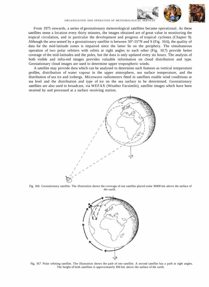
ORGANIZATION AND OPERATION OF METEOROLOGICAL SERVICES 97
From 1975 onwards, a series of geostationary meteorological satellites became operational. As these satellites sense a location every thirty minutes, the images obtained are of great value in monitoring the tropical circulation, and in particular the development and progress of tropical cyclones (Chapter 9). Although the area sensed by a geostationary satellite is between 50°-55°N and S (Fig. 10.6), the quality of data for the mid-latitude zones is impaired since the latter lie on the periphery. The simultaneous operation of two polar orbiters with orbits at right angles to each other (Fig. 10.7) provide better coverage of the mid-latitudes and the poles, but the data is only updated every six hours. The analysis of both visible and infra-red images provides valuable information on cloud distribution and type. Geostationary cloud images are used to determine upper tropospheric winds.
A satellite may provide data which can be analysed to determine such features as vertical temperature profiles, distribution of water vapour in the upper atmosphere, sea surface temperature, and the distribution of sea ice and icebergs. Microwave radiometers fitted in satellites enable wind conditions at sea level and the distribution and type of ice on the sea surface to be determined. Geostationary satellites are also used to broadcast, via WEFAX (Weather Facsimile), satellite images which have been received by and processed at a surface receiving station.
Fig. 10.6 Geostationary satellite. The illustration shows the coverage of one satellite placed some 36000 km above the surface of the earth.
Fig. 10.7 Polar orbiting satellite. The illustration shows the path of one satellite. A second satellite has a path at right angles. The height of both satellites is approximately 850 km above the surface of the earth.

98 METEOROLOGY FOR SEAFARERS
GLOBAL TELECOMMUNICATIONS SYSTEM
The degree of effectiveness of any NMC depends not only upon the efficiency of its own national observing network, but also on data from other sources.
In 1968, World Weather Watch (WWW) was established to encourage the rapid and efficient exchange of data. An important component of WWW is the Global Telecommunications System (GTS) (Fig. 10.8) through which observations and processed information are transmitted. A main telecommunication network interconnects three primary centres, Washington, Moscow and Melbourne, with regional hubs. The regional hub is the major link between the network and a number of National Meteorological Centres (NMC), each centre collecting and processing observations from its land observing network, and voluntary observing ships on the adjacent seas. In this way a NMC can not only receive any data required but also use the GTS to disseminate data to other centres.
Fig. 10.8 Global Telecommunications System.
DATA ANALYSIS
Analysis of surface and upper air observations produces synoptic charts which are a necessary preliminary to forecasting. Observations received at a NMC are fed into a computer system which checks them for any inaccuracies, a large volume of data being processed in a relatively short period. The computer system then presents the data in the form required by the forecaster.
Surface Synoptic Charts
Surface synoptic reports are plotted by the computer using the station model format (Figs. 10.9 and 10.10), and the forecaster then analyses the plots in order to construct a surface synoptic chart, also termed a surface analysis. Isobars are drawn to establish the distribution of atmospheric pressure at mean sea level, and hence the major pressure systems existing at the synoptic hour (Fig. 10.11). With the aid of satellite images (Fig. 10.5) fronts are then drawn on the chart (Fig. 10.12). At each stage of the analysis a comparison is made with the previous synoptic chart to confirm the feasibility of the features established.


100

ORGANIZATION AND OPERATION OF METEOROLOGICAL SERVICES 101
While the area covered by, and the frequency of surface analyses will vary from one NMC to another, charts are generally produced for the major synoptic hours of 0000, 0600, 1200 and 1800 UTC for the local regional area (e.g. British Isles and W Europe), or for a larger area (e.g. N Atlantic and W Europe—Fig. 10.12). Circumpolar surface synoptic charts giving a broader view of the distribution of pressure systems are also constructed (Fig. 10.13). In addition to the above, surface synoptic charts may also be produced for intervening synoptic hours, 0300, 0900, 1500 and 2100 UTC, which generally cover the local regional area for which synoptic reports, mainly from land observing stations, are available.
Fig. 10.13 Circumpolar surface synoptic chart.
Upper Air Charts
Upper air data collected at 0000, 0600, 1200 and 1800 UTC are transmitted to a NMC where they are checked by the computer. A number of charts can then be produced to illustrate various aspects of the upper atmosphere. One example is the contour chart for a given pressure level. In Fig. 10.14, the contour lines indicate the heights above mean sea level at which atmospheric pressure is 500 hPa. The chart is a topographic representation of the 500 hPa level which shows a wave pattern whose amplitude and wavelength can be determined. Similar charts for other pressure levels may also be constructed, and the characteristics of jet streams determined from plotted wind data.
Upper air data is also used to compile thickness charts, the term referring to the vertical separation between two selected pressure levels. A common example is the 1000-500 hPa thickness chart (Fig. 10.15) on which the vertical separation is shown by contours termed thickness lines. Thus the chart indicates the distribution of warm air relative to cold air, as the vertical separation is dependent upon the mean temperature of the air column between the two levels.
Both the contour and thickness charts illustrate the background details which play a critical role in the existence of the features shown on surface synoptic charts, and thus provide important and valuable information in the production of a forecast.


ORGANIZATION AND OPERATION OF METEOROLOGICAL SERVICES 103
Nephanalysis
Nephanalysis is the interpretation of visible and infra-red satellite images ("nephos" is the Greek word for cloud). Charts can be produced which identify cloud types using the basic categories of stratiform, cumuliform and cirriform. They also indicate the amount of cloud present and, in some cases, an estimate of base height. Major vortices (cyclones and anticyclones) can be identified. The characteristics of cirriform cloud may assist in locating the position of a jet stream and indicate the existence of clear air turbulence (CAT).
FORECASTING TECHNIQUES
Numerical Models
The production of forecasts involves the use of computers and numerical models, which are a series of equations representing the existing state of the atmosphere and its subsequent evolution over a given period. L. F. Richardson, a British meteorologist, devised and used the first numerical model in 1922 to produce a forecast for the area covering the British Isles and Europe. Apart from imperfections in the design of the model, which produced an excessively large pressure change for the forecast period (145 hPa in 6 hours), there was the major disadvantage of the time involved in the production of the forecast. The introduction of the electronic computer in the 1950s overcame this problem and numerical models are now part of the forecasting process.
In a numerical model the characteristics of the atmosphere are defined for a number of levels, each level being subdivided by a grid system covering a particular geographical area. The early UK model used three levels with a separation of 300 km between grid points. Greater computer power has permitted an increase in the number of levels, a decrease in distance between grid points, and an expansion of the geographical area. These refinements have improved the accuracy of forecasts. The UK Meteorological Office currently uses a global model, which has a coarse mesh. Simultaneously models covering the North Atlantic and Western Europe, and the United Kingdom are used to provide more detailed forecasts for this area.
The operation of a model depends upon an accurate input of data to determine the initial state of the atmosphere. Data from upper air soundings and analysed satellite data, particularly temperature profiles, are fed into the computer. The computer then calculates a number of characteristics of the atmosphere for each grid point at pre-determined time steps (e.g. 10 minutes) over the complete period of the forecast (e.g. 24, 48, 72, 96 and 120 hours). In the development and operation of the global model, the UK office has taken into account upper air soundings which are synoptic, and satellite data which may well be asynoptic. The data produced by the model is compared with the synoptic data for compatibility, and the latter is then incorporated into the forecasting process.
The operation of a numerical model also depends upon the input of data which includes the radiation budget of the atmosphere, and the nature of the earth's surface which affects the flux of water vapour to the atmosphere. However, present models are limited by the techniques involved and the availability of data.

104 METEOROLOGY FOR SEAEARERS
Prognostic Weather Charts
The computer generated forecast data is used to produce prognostic (forecast) charts for the surface (Fig. 10.16), and a number of pressure levels in the upper atmosphere. The forecaster then draws fronts on the surface prognostic chart with the aid of the computer output of forecast precipitation at the surface. The final surface prognostic chart is the outcome of the interpretation of the forecast data generated by the computer, the comparison of the prognostic chart with previous synoptic charts, and the forecaster's assessment of the prognostic situation. Thus every prognostic chart is the combined production of computer and human skill, the man-machine mix.
The period ahead for which forecasts have been produced has gradually been extended. The forecast by L. F. Richardson was for a very short period compared with the 24 to 36 hour forecasts of the early operational models. Currently operational forecasts are produced for periods in excess of 5 days ahead, and work continues on improving the models.
Fig. 10.16 Computer output for a surface prognostic chart.


METEOROLOGY FOR SEAFARERS
The effectiveness of the routeing service depends upon the availability to the organization of ship, cargo and relevant operational data. Generally, a representative of the organization visits the ship to collect this information, and discuss the routeing service with those on board. Ship data include the ship type, draught, trim, stability and speed made good relative to sea conditions (wind waves, swell and current). This information is normally extracted from the deck log, or, if not available, obtained from a similar type of ship. The organization then constructs for each state of loading a set of performance curves related to the important characteristics of wave height and relative direction (following, beam or head seas) (Fig. 10.18). It should be noted that the style of presentation of performance data varies from one organization to another.
For each voyage, the cargo data may relate to factors such as routeing to avoid certain atmospheric conditions, or a deck cargo may need to be protected from continuous heavy seas. Operational factors include fuel economy, schedules demanded by the charterer, and limitations arising from insurance clauses. Thus each passage has a prime objective which may be least time on voyage (usually the objective in the early days of weather routeing), least damage to cargo or vessel, or maximum fuel economy (significant from the early 1970s).
Route Selection
The initial route selected takes into account the objective of the passage and the environmental conditions likely to be encountered in the area through which the ship will pass. The environmental conditions are established from synoptic and prognostic surface and upper air charts. Major pressure systems, whether depressions, anticyclones or tropical cyclones, their direction and speed of movement, development and decay are determined. Thus the critical features of wind direction and speed, icing or reduction of visibility due to fog or heavy precipitation, are assessed together with a general appreciation of the future sea state. At this stage, synoptic and prognostic data relating to sea ice and icebergs, ocean currents from current atlases and other environmental factors are considered.

ORGANIZATIONAL AND OPERATION OF METEOROLOGICAL SERVICES
If the objective is least time, then the initial route is further evaluated by plotting either side of this route a total of five or six alternatives, 10° to 15° apart (Fig. 10.19). The speed likely to be made good along each route is determined by referring to the forecast conditions of wave height and direction from the wave prognostic chart, and relating these to the performance curves (Fig. 10.18). Allowance is made for the set and speed of any current along the route, and the vessel's predicted distance made good over the next 12 hour run is then plotted. Thus in 12 hours the vessel could be in any one of six positions which lie on a locus (Fig. 10.19). The technique is repeated for each 12 hour period ahead for which there is prognostic wave data, and a set of loci is thus plotted. A point is then selected which is nearest to the destination (Fig. 10.19), and an advised course and speed is established which would bring the vessel to that point in the least time. As the routeing organization receives more up to date wave prognostic data, so the procedure is repeated and the advised route confirmed or modified.
The least time technique is thus the optimization of all environmental factors to ensure the fastest passage by the particular vessel. However, it must be emphasized that if other objectives are important then this technique may have to be modified.
Communications
The advised route and speed is passed to the vessel before departure, and during the passage communications are maintained at intervals dictated by the reassessment of the advised route. The messages passed may also contain a summary of the synoptic and prognostic atmospheric and sea state conditions. Costs incurred for the service generally cover the fee for the advice provided and the cost of transmissions.
The progress of the vessel is monitored continuously either through synoptic reports it makes, if it is a voluntary observing ship, or through the position reports made at intervals (usually 24 or 48 hours), which are recommended by the routeing organization. The latter reports usually include a brief summary of atmospheric and sea state conditions. In addition to these the vessel must report unforeseen circumstances (e.g. breakdown, alterations of course or speed).
Voyage Analysis
On completion of the voyage an analysis may be carried out by the routeing organization. A synopsis of the voyage is produced in terms of meteorological and sea state conditions, and performance of the vessel over the route followed. The voyage analysis, which is made available to the vessel and the owner, often incorporates a summary of an alternative route which may have been considered.
The assessment of the benefits gained from ship routeing are by no means easy and various techniques are used. One method is to compare the overall expenditure of the vessel when routed with that prior to routeing. A second method is to compare the time saved by the routed vessel with that of an unrouted one during the same period (Fig. 10.20).


CHAPTER 11
FORECASTING SOURCES
While the seafarer can do nothing to control the atmospheric and sea conditions affecting his vessel, he can indirectly influence the circumstances arising from them through careful evaluation and application of forecast data both in pre-passage planning and on passage. The success or otherwise of the evaluation and application depends upon the amount and quality of data available.
SINGLE OBSERVER FORECASTING
Observations and Analysis
Whether on passage or in port the seafarer can directly monitor his environment to a greater or lesser degree, depending upon the range of facilities and the time available. By analysing a comprehensive series of observations (Table 11.1) trends can be established, from which the recent history of the atmosphere and sea conditions can be determined. As an example, pressure tendency, not necessarily restricted to the standard three hours preceding the time of observation, can be assessed from the barogram (Chapter 2), or established to the nearest hectopascal by frequent reading of the simple aneroid barometer. Trends can also be assessed of the visibility range, cloud amount, and sequence of cloud type. The value of visibility trends are enhanced when related to the presence and intensity of precipitation, mist, fog, haze or the sea state. The tendency of the wind to back or veer, and the speed to increase or decrease can be determined, and the characteristics of swell are also worth noting (Chapter 9).
Forecast
The analysis of the data in Table 11.1 indicates the advance of a frontal depression, and the bearing of the centre can be determined by applying Buys Ballot's Law. Thus conditions likely to be encountered will be those associated with the passage of such a depression (Chapter 8). Once such a short term forecast is made, the monitoring process should be continued to verify or modify the forecast at frequent intervals, as the conclusions reached will be important for a safe passage.
The above procedure has inherent limitations, as it assumes that the particular pressure system inferred from the observations will result in the same meteorological conditions on every occasion.
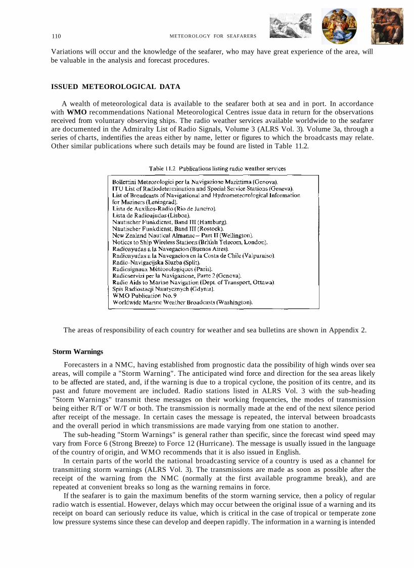
110 METEOROLOGY FOR SEAFARERS
Variations will occur and the knowledge of the seafarer, who may have great experience of the area, will be valuable in the analysis and forecast procedures.
ISSUED METEOROLOGICAL DATA
A wealth of meteorological data is available to the seafarer both at sea and in port. In accordance with WMO recommendations National Meteorological Centres issue data in return for the observations received from voluntary observing ships. The radio weather services available worldwide to the seafarer are documented in the Admiralty List of Radio Signals, Volume 3 (ALRS Vol. 3). Volume 3a, through a series of charts, indentifies the areas either by name, letter or figures to which the broadcasts may relate. Other similar publications where such details may be found are listed in Table 11.2.
The areas of responsibility of each country for weather and sea bulletins are shown in Appendix 2.
Storm Warnings
Forecasters in a NMC, having established from prognostic data the possibility of high winds over sea areas, will compile a "Storm Warning". The anticipated wind force and direction for the sea areas likely to be affected are stated, and, if the warning is due to a tropical cyclone, the position of its centre, and its past and future movement are included. Radio stations listed in ALRS Vol. 3 with the sub-heading "Storm Warnings" transmit these messages on their working frequencies, the modes of transmission being either R/T or W/T or both. The transmission is normally made at the end of the next silence period after receipt of the message. In certain cases the message is repeated, the interval between broadcasts and the overall period in which transmissions are made varying from one station to another.
The sub-heading "Storm Warnings" is general rather than specific, since the forecast wind speed may vary from Force 6 (Strong Breeze) to Force 12 (Hurricane). The message is usually issued in the language of the country of origin, and WMO recommends that it is also issued in English.
In certain parts of the world the national broadcasting service of a country is used as a channel for transmitting storm warnings (ALRS Vol. 3). The transmissions are made as soon as possible after the receipt of the warning from the NMC (normally at the first available programme break), and are repeated at convenient breaks so long as the warning remains in force.
If the seafarer is to gain the maximum benefits of the storm warning service, then a policy of regular radio watch is essential. However, delays which may occur between the original issue of a warning and its receipt on board can seriously reduce its value, which is critical in the case of tropical or temperate zone low pressure systems since these can develop and deepen rapidly. The information in a warning is intended

FORECASTING SOURCES
to establish concisely the forecast conditions for the sea area concerned, but it must be interpreted intelligently using onboard observations and other data, as it may only be applicable to part of the area.
Weather Bulletins
National Meteorological Centres also issue data in the form of weather bulletins for vessels at sea. As with storm warnings the channels used are the radio stations, and the operating frequencies, times, and method (W/T) of transmission are listed in ALRS Vol. 3 under the sub-heading "Weather Messages". Whilst the nature of bulletins varies around the world, WMO does recommend a certain range and order of presentation of data. A bulletin may consist of six parts (Table 11.3). Parts 1, 2 and 3 contain the important data, usually in the language of the country of origin, but may be repeated in English and the terminology used normally follows WMO guide-lines. If Parts 4, 5 and 6 are included, they may be transmitted with Parts 1, 2, and 3, or at a later time. The number of times a bulletin is issued in 24 hours will vary from one source to another.
Tabic 11.3 Structure of a weather bulletin
Part
1
2
3
4
5
6
Title
Storm Warnings
Synopsis
Forecast
Analysis or prognosis
Sea station reports
Land station reports
Contents
Sea areas affected identified, forecast wind conditions, and the location, movement, development or decay of the related pressure centres. The statement of "No Storm Warnings" is used when there is no forecast storm condition.
Identifies the major pressure systems, their movement, development or decay. In low latitudes this part may simply state the existence of seasonal weather, the daily condition being similar to the seasonal pattern and the rate of change minimal.
A forecast statement for the period stated in the bulletin for each of the sub-sections for which the NMC is responsible. The statement includes the anticipated wind, visibility, weather and wave conditions.
Details of type and location of pressure centres, central pressure values, types and location of fronts, and position of selected isobars. The data is in coded format using the IAC FLEET Code (an abbreviated form for marine use of the International Analysis Code (IAC)).
Synoptic reports from vessels in a reduced code format.
Synoptic reports from coastal land stations in a reduced code format.
As an example, the Atlantic Weather Bulletin, comprising Parts 1, 2 and 3, is issued by United Kingdom Meteorological Office via Portishead Radio (Table 11.4(1)). The bulletin covers the area within 35°N to 65°N and 15°W to 40°W, which is divided into six sections, and also the sea areas of Sole, Biscay, Finisterre, Trafalgar and the Norwegian Sea and Denmark Strait (Fig. 11.1). Data for adjacent zones may be included in the bulletin if it is likely to have a significant bearing on the future meteorological conditions within the forecast area. The bulletin is broadcast at 0930 and 2130 UTC.
If a weather bulletin contains Part 4, then it can be decoded and a surface analysis plotted. The chart will indicate all the major synoptic features and others which are not specifically mentioned in Part 2 of the bulletin.
The seafarer, having plotted a surface analysis or received one by facsimile, can generate an outline of the prognostic situation by replotting pressure centres and related fronts, whose details of movement are contained in Part 2 of the bulletin. The forecast data of Part 3 of the bulletin can then be related to the movement, development, or decay of the systems.
i

The total time involved in the issue, receipt, decoding and plotting of a bulletin which contains Part 4 is worth reviewing. The completed chart is several hours old, and this factor may be significant when the synoptic situation is changing rapidly. However, the critical aspects of such a situation should be identifiable at an earlier time from Parts 1 and 2.
Weather bulletins are also issued as part of the Global Marine Distress Safety System (GMDSS). The format is the same as for Parts 1, 2 and 3 of a weather bulletin (Table 11.3). An example is the High Seas Weather Bulletin issued by the UK Meteorological Office (Table 11.4(2)). The forecast areas for this bulletin are illustrated in Fig. 11.2.
Maritime Forecast Code
National Meteorological Centres may issue bulletins in their own language only, and repeat the information using the Maritime Forecast Code, the coded message being prefixed by MAFOR. The area to which the forecast applies is identified by an indicator figure or geographical name. The period for


METEOROLOGY FOR SEAFARERS
which the forecast is valid and the mean forecast values for a number of meteorological elements are given in code format. The significant elements are surface wind and weather (e.g. precipitation, fog, mist, ice accretion, visibility). Forecast data relating to sea state, air temperature and swell may also be included. In a transmission these elements may be considered more than once so describing any changes which may occur and their duration. Thus the forecast may cover a period up to 72 hours ahead, which is of value to the seafarer when related to the assessment of onboard observations.
Shipping Forecast
The UK Meteorological Office issues a shipping forecast for coastal areas, which is broadcast by the British Broadcasting Corporation (BBC) on Radio 4. The contents of the transmission include gale


METEOROLOGY FOR SEAFARERS
warnings, a general synopsis (with comments on future change), a forecast for the next 24 hours of the wind, weather and visibility for each coastal area and the latest reports from a number of coastal stations. The forecast is issued four times daily, and provides in greater detail the anticipated conditions for sea areas around the British Isles (Fig. 11.3), which are not available in the Atlantic Weather Bulletin.
For inshore waters (up to 12 miles offshore) forecasts of wind, weather and visibility are broadcast on BBC Radio 4. Synoptic reports from a selection of observing stations are included in the Radio 4 broadcasts. These forecasts are valuable both to the seafarer and to those involved in recreational activities.
Fig. 11.3 Shipping forecast areas.
Navigational Warnings
Meteorological warnings of conditions affecting safety of vessels may either be included in the NAVAREA warnings or precede their issue (ALRS Vol. 3). The phenomena which may form a part or all of the broadcast may be tropical cyclones, visibility of 2 km or less, severe icing, wave heights of 8 m or more, and winds of Force 10 or above. Gale warnings, weather forecasts and ice reports are also transmitted via NAVTEX (ALRS Vol. 3).


METEOROLOGY FOR SEAFARERS
FACSIMILE CHARTS
Equipment
The provision of meteorological data through facsimile transmissions is a relatively recent introduction compared with the issue of weather bulletins. Several companies manufacture and market facsimile equipment which essentially consists of a receiver and a recorder (Fig. 11.5). When the receiver is tuned to the frequency of the transmission, the data is recorded normally in chart form on special paper which feeds through the recorder. The seafarer, by consulting ALRS Vol. 3 and identifying those stations with subheading "Facsimile Schedule" which transmit the data required, selects the frequency on the receiver together with the automatic mode on the recorder, if available. If the recorder is in the automatic mode, it is activated by the initial signal transmitted which also sets the drum speed (revolutions per minute) and index of co-operation (a term relating to the line scanning of the equipment). The recorder is also stopped automatically at the end of the transmission. If there is no automatic mode, the operator must set the recommended drum speed and index of co-operation. When the transmission begins the recorder is started, and the alignment of the paper checked and adjusted if necessary so that the chart is printed as a single entity. The equipment must be stopped manually at the end of the transmission. However, it should be noted that the procedure for operating facsimile equipment varies and operating manuals should always be consulted.
Although the total time taken for a chart to be transmitted will depend upon its size, the receipt of information by this means is less time consuming than the receipt and plotting of a weather bulletin, and sources of error in transmission and subsequent decoding are minimised or eliminated. However, the availability of facsimile data does not render bulletin data obsolete, a point which will be discussed later.
(1) Receiver FAX-207 (Furuno). (2) Receiver FAX-210 (Furuno). Fig. 11.5 Facsimile equipment.
Surface Analysis The facsimile schedules in ALRS Vol. 3 provide information on the types of charts available from
meteorological centres. Of those listed, the surface analysis and surface prognostic charts are of particular value to the seafarer. The surface analysis shows the surface distribution of pressure by means of isobars and associated fronts for the synoptic hour stated (Fig. 11.6). Synoptic reports from land stations and ships may also be included using the recommended station plot format, or, if there is insufficient space, only critical elements may be plotted (e.g. wind direction and speed). Although the

FORECASTING SOURCES 119
chart is essentially synoptic in nature, prognostic data for direction and speed of movement, and central pressure values of pressure centres may also be included. Retrospective data for pressure centres, a horizontal distance scale, and a geostrophic wind scale may also be shown. The chart projection is usually given and, for clarity and quick reference, latitude and longitude intersections are plotted at frequent intervals. If the chart is a preliminary analysis, the data shown is that of isobars which illustrate the major pressure systems.
The area covered by a facsimile surface analysis varies from one transmitting source to another, and the seafarer can check its limits from the schedule. Surface analyses from any one source may cover different areas, and while a few meteorological offices may issue one chart daily, most issue at least two, one for 0000 UTC and one for 1200 UTC. Generally the number of charts issued is greater for the immediate area of interest to the meteorological office compared with the number covering a larger horizontal area. For example the UK Meteorological Office issues surface analyses covering its immediate area of interest (Fig. 11.6) for 0000, 0600, 1200 and 1800 UTC, while the circumpolar chart is only issued for 0000 UTC.
Prognostic Charts
Surface prognostic charts show the anticipated distribution of surface pressure by means of isobars and related fronts for a future time, which is noted in its title. Fig. 11.7(1)—(3) are examples of the range of surface prognostic charts issued by the UK Meteorological Office which are listed in the facsimile schedule in ALRS Vol. 3. As with the surface analysis, the issue of prognostic charts varies from one source to another. Generally the 24 hour surface prognosis is issued at least once daily, and in some cases four times daily for the synoptic hours 0000, 0600, 1200 and 1800 UTC. However, surface prognostic charts for times in excess of 24 hours are usually issued only once daily. It should also be noted that,


although a degree of continuity of area is maintained for the more important charts, the area covered by a 24 hour surface prognostic chart may not be the same as that of the 36 hour chart from the same source.
Facsimile prognostic data from some sources may not be presented in the form described above. Instead a surface prognostic chart may show the anticipated wind direction and speed for a number of sea areas by means of symbols, and significant weather conditions in plain language. Plain language prognostic and synoptic statements may also be issued via the facsimile system.
Other Charts
A number of other charts may be available to the seafarer through facsimile transmissions. Among them are the wave analysis and wave prognostic charts, the latter being for 24 and 48 hours (Fig. 10.17). Ice charts, whose transmission schedules are to be found in ALRS Vol. 3, may include data relating to sea ice, icebergs and sea surface temperature (Fig. 11.8). Certain ice charts may only show synoptic data but on others prognostic data may be included, as with those issued by the International Ice Partol. Ice charts can usually be supplemented by bulletins from a number of sources which are listed in ALRS Vol. 3.
Satellite images or nephanalyses are issued by some meteorological centres (Chapter 10). A limited number of centres may issue radar summaries, data on surface ocean currents, and ocean thermal analyses.

Fig. 11.8 Sea ice chart.
UTILIZATION OF FACSIMILE DATA
Facsimile transmissions are a potential source of a large volume of data which can be incorporated into passage planning. In order to gain the benefits of the data, a careful study of the transmission schedules is necessary. However, the suitability or otherwise of the data may only become apparent when the actual charts have been received.
Surface analyses and prognostic charts received by the seafarer may be studied individually and then compared, thus establishing the state and the likely evolution of the atmosphere in terms of pressure systems, their movement, development and decay. A review of Fig. 11.6 and 11.7 (1-3) illustrates the case. At 0000 UTC on the 17th December 1984 the surface analysis (Fig. 11.6) shows that the area of the N Atlantic west of Ireland is under the influence of a westerly airstream. A comparison of Fig. 11.6 and Fig. 11.7(1), the 24 hour surface prognosis, indicates that at 0000 UTC on the 18th December 1984 frontal depression (LD) is forecast to be at 57°N 45° W with a central pressure value of 972 hPa. A comparison of the 24 and 48 hour surface prognostic charts (Fig. 11.7(1) and (2)) shows that during the intervening period the system is expected to move north-eastwards, deepen and begin to occlude, with its centre WSW of Iceland (62°N 27°W) at 0000 UTC on the 19th December 1984. At that time the warm front may be positioned along the west coast of Ireland, the cold front extending to the south and south-west of the centre, thus influencing the weather in the eastern half of the N Atlantic.
The progress of this frontal depression in the following twenty-four hours can be traced by comparing the 48 and 72 hour surface prognostic charts (Fig. 11.7(2) and (3)). Thus at 0000 UTC on the 20th December 1984, the frontal depression is likely to be positioned at 67°N 11 °W, having begun to fill and continued to occlude. The speed of advance of the centre will have decreased in comparison with

FORECASTING SOURCES
that of the preceding forty-eight hours, with the warm and cold fronts continuing to progress rapidly eastwards.
The 72 hour surface prognostic chart (Fig. 11.7(3)) also indicates the development of a frontal depression (54°N 18°W) on the trailing cold front of LD. The progress of this system can be monitored on future facsimile prognostic charts as they are received. This type of system is particularly significant since it moves rapidly eastwards and simultaneously deepens, resulting in adverse conditions across the British Isles and adjacent sea areas.
The information extracted from the surface analyses and prognostic charts may be supplemented with information from other facsimile charts. For example the wave prognostic chart will define the anticipated wind and swell wave conditions over an ocean area (Fig. 10.17), and satellite images or nephanalyses will show the associated cloud forms as they develop.
As with weather bulletin data, the updating of all facsimile charts is important and relatively easy with the frequent transmission of data. Thus within twenty-four hours of receiving a 72 hour surface prognostic chart the seafarer will receive a 48 hour chart. The latter will be more reliable in terms of its representation of the future state of the atmosphere, a factor reflecting the limitations of the numerical models to forecast accurately for extended periods.
Facsimile data and weather bulletins can be regarded as being complementary. The plain language forecast (Part 3) of the bulletin is a more detailed summary of forecast weather conditions for areas of the ocean, in terms of variations of wind speed and direction, precipitation and visibility, whilst the surface prognostic charts show the future position of pressure systems and fronts. Thus the details of the forecast in the bulletin amplify the data derived by comparing the surface analysis and 24 hour prognostic chart.
Finally it should be stressed that, notwithstanding the availability of both bulletin and facsimile data, the direct observation of the immediate environment should not be forgotten; it should be used to assess the accuracy of both types of data, and thus interpret and modify the forecast.
CLIMATIC DATA
Routeing Charts
Routeing charts for the oceans are published by many organizations and Table 11.6 lists the data which is based on observations collected over a number of years. The charts present a summary of the
Table 11.6 Routeing chart data
Climatic conditions
Air pressure, pressure systems
Surface wind
Air, sea surface, temperatures and dew-point temperatures
Visibility
Tropical cyclones
Surface currents
Sea ice and icebergs
Presentation
Isobars and, in some cases, frequencies of deep depressions with depiction of storm tracks.
Frequency distributions of wind direction in 8 points of the compass (wind rose) and wind speed, frequencies of gales and storms.
Isotherms of mean values.
Frequencies of visibility.
Tracks of individual cyclones and distribution for the months of the year.
Predominant direction and rate of current.
The geographical distribution of sea ice and icebergs.

METEOROLOGY FOR SEAFARERS
climatic conditions for a particular month in a standard form (e.g. mean pressure distribution shown by isobars), and also use graphical and numerical forms of presentation. Some of the data may be shown on inset charts and tables.
Sailing Directions
Sailing directions or pilot books also include climatic data on conditions at sea and climatic tables for observing stations in coastal areas. Information on mean pressure distribution for certain months, wind roses, winds of Force 7 or greater, tracks of depressions and tropical cyclones, reduced visibility, and fog are presented in chart form. The supporting descriptions summarise the charts and provide additional data on cloud, precipitation, thunderstorms, air temperatures, relative humidity, fronts and local winds. Ocean currents, sea and swell conditions, sea surface temperature, and ice are included.
Although the data from both routeing charts and sailing directions are climatic in nature, they are of value to the seafarer. However, intelligent interpretation of the data is needed, particularly in those areas where the weather conditions change frequently over relatively short periods.
If the seafarer makes full use of on board observations, weather bulletins, facsimile services and climatic data, then he will have the best information possible to ensure the safe passage of his vessel.

Chapter 9 discussed tropical cyclones and suggested a guide for ships. The account below, reproduced by kind permission of the US Mariners Weather Log (vol. 27), highlights the advanced warning provided by the swell, which in this case was violently emphasized by an extreme storm wave, and the real danger and difficulties encountered at sea by vessels entering a tropical cyclone. The ship's barogram is included in Chapter 2, but other photographs of damage, which were included in the article, have been omitted.
SS MOBILE AND TYPHOON FAYE
The following is a summary of Captain Cordes' account of his voyage from Kaoshing, Taiwan, to the US Naval Base, Subic Bay, Philippine Islands in ss MOBILE. Times are LMT.
"The MOBILE departed Kaoshing at 0742 on 23 August, 1982, for Subic Bay. A full profile of containers was aboard with truck chassis in bundles of two lashed on top of the containers on hatches No. 1, No. 2, and No. 9. Wooden 4 x 4's were laid across the tops of the containers to distribute the load of the chassis.
The MOBILE proceeded along the west coast of Luzon, which reduced the general height of the sea from the easterly wind. The weather broadcast from Hong Kong located Typhoon Faye 13°N 118°E at 0500 on 24 August, 1982, and forecast it to remain essentially stationary for the next 24 hours. There was no evidence of the typhoon other than a slowly increasing southerly swell.
At 1500 on 24 August the ship was struck by an extreme storm wave. The ship pitched steeply down into the trough ahead of the wave, slammed into the wave, and pitched upward rapidly. When the wave passed under the stern, the MOBILE was again slammed into the sea. After a short period of violent pitching the ship began to ride normally again. This occurred at 15°09'N, 119°52'E. A container on hatch No.l burst open and some of the mail bags were washed over the side when the extreme wave came aboard. A contributing factor to the damage was the large moment arm of the heavy chassis on the top of the containers well forward of the ship's centre of movement. When the violent pitching and slamming occurred, the chassis became like huge hammers.
At about 1600 the US Military Sealift Command at Subic Bay was contacted for the latest weather forecast. Typhoon Faye's position was the same. It was expected to pass Subic 60-70 miles to the west at its closest point of approach at about 2300. Speed was reduced to allow better reaction to any other extreme waves that might be coming and the vessel proceeded on course to Subic, anticipating arrival about 1900, well ahead of the typhoon.
At 1630 the weather was good, light overcast of the usual monsoon type, the wind was east-northeast at 10-15 knots, and there was a moderate southerly swell. By 1700 the wind had increased to 50 knots and an ominous line of low dark clouds appeared on the horizon ahead. Typhoon Faye had not been stationary at all, but had continued to move northeastward at about 15-20 knots since the morning report.
It was fortunate that the wind was from the east because the MOBILE was only three miles west of Capones Island. A westerly course was tried to get the ship away from land in anticipation of the wind reversing direction on the opposite side of the typhoon eye.
At 1730, the wind was from the east at more than 60 knots and the barometer was dropping

METEOROLOGY FOR SEAFARERS
precipitously. The ship would not hold a westerly course in the wind and high sea and swell. The ship's head fell off to the southwest, and at 1805 maximum speed was needed to hold the southwesterly course. A fully-loaded container ship in a storm has all the attributes of a square-rigged sailing ship with all sails set.
Blinding rain reduced visibility to zero and made the radars ineffective and by 1830, the wind speed had increased to a steady 80-90 knots with gusts estimated at 100 knots. However, the ship was now riding well with wind and sea on the stern. Speed cautiously reduced to the minimum for steerage. Both radar antennae refused to turn in the high wind.
At about 1945 (1145Z) the MOBILE entered the eye of the typhoon. One radar began functioning and the eye could be clearly seen encircling the ship, but the heavy rain of the storm attenuated the radar so that targets beyond the eyewal! could not be detected. The Loran C gave a reasonable fix (within five to six miles in this area). To avoid any chance of grounding, it was decided to maintain the southwesterly course. The position of the eye of the typhoon was transmitted to Hong Kong and they responded with typhoon advisory No. 12 relocating Typhoon Faye. At about the same time the ss PRESIDENT POLK, 20 miles to the northeast, reported 80-knot winds.
At about 2030 the MOBILE entered the southern wall of the eye. The wind jumped to an average steady wind of 80-90 knots with gusts well over 100 knots. Spray and torrential rain reduced visibility to near zero and seas were mountainous. The radar ceased functioning again as the wind increased. Many of the ship's parts and fittings could be seen blowing or bending in the wind with water coming across the ship. The masthead and range lights were lost around 2045. Finally, the storm began to decrease about 2130 with wind under 50 knots and, for the remainder of the night, the wind gradually decreased.
The following is a list of the damage:
(a) Six chassis lost overboard (b) Four chassis damaged (c) Four containers destroyed on No. 1 hatch (d) Eight containers on No. 2 hatch damaged (e) Both masthead and range lights destroyed (f) HF radio antenna bent back 45 degrees (g) All wire antennae destroyed (h) Both cranes inoperative (i) Anchor windlass controller sheared off at deck level (j) Vent pipe sheared off allowing bosun's stores over No. 2 deeptank to flood with 3 ft of water."
This account was published again in Seaways, May 1984, from whom the permission has been given to publish the comments of Captain E. W. S. Gill:
'The remarkable thing regarding this incident is that even in this era of space-age technology, the position of tropical cyclones cannot be guaranteed. In this particular case the typhoon was surely within strategic radar range of the US Naval Base at Subic Bay, as well as any strategic radars at Manila. Yet the actual position and movement of the storm was undetected until the MOBILE reached the centre, and confirmed it".
It also emphasises the importance of an accurate predicted pressure inside the cyclone. This can be of inestimable value to a seaman in determining the position of one's ship, relative to the storm. Personally, I have always endeavoured to get below (equatorially) a tropical cyclone, rather than rely upon a steady predicted movement of the cyclone as indicated by meteorological reports. It's safer.
The comments in the article regarding the inability of even large and powerful container vessels to manoeuvre as one desires, once the storm has a ship in its grip, can be vouched for by myself. I had previously noted that container vessels with their large windage areas can be extremely difficult to keep on course that would normally be best for the ship under the hurricane force weather conditions.
With a quarterly wind and sea, the tendency for the ship to try to broach to is enormous. The large application of helm to prevent the ship turning has the counter affect of slowing the ship down and losing steerage way so that it is imperative that the steering be closely watched under these conditions.
With the same strength of wind and sea from ahead there is again the tendency for the ship to pay off the wind rather violently, and any increase of speed merely increases the pounding effect. The only thing to do under these circumstances, and providing there is sufficient sea room, is to cut and run only never

TYPHOON FAYE AND EXTREME STORM WAVES
leave it too late to make this decision, for the turning of a ship in tumultuous sea, combined with extreme wind heel factors could put the ship over to an impossible angle.
EXTREME STORM WAVES
Extreme Storm Waves (ESW), one of which struck ss MOBILE, arise from the combined effects of meteorological and oceanographic conditions (Plate 44). The following table, produced by the US National Weather Service, is a guide to the different types of waves.
Table Al Classification of extreme storm waves
Description
Steep, white water on crest; "hole-in the-sea" in front; usually occurs as a single large wave aligned with other waves in the seaway.
Group of large waves-usually three, with the second wave being highest. The group is aligned with other large waves in the seaway.
Group of large waves, usually three, misaligned by 30 degrees or more to local wind-driven seaway.
Large breaking wave(s) intruding into local seaway at angles up to 50 degrees from direction of local wind driven seaway; of unusual height with respect to other waves in the local seaway.
Comment
Known to occur in strong, increasing winds. Tend to reoccur as "every 7th wave" among the larger waves in the seaway. These large, steep waves are apt to cause local damage to a ship or its lifeboats, accommodation ladders etc.
Likely to occur in strong winds which have peaked or begun to decrease in strength. During the period of peak winds these waves are apt to be much higher than the other large waves in the seaway. This wave group can produce severe hull girder bending stresses.
Wave group intrudes unexpectedly into local seaway and produces locally high wave crests at intersections with the largest waves in the local wind-driven seaway. The wave group tends to cause severe roll response by a ship.
Frequently characterized as a "rogue" wave(s). Very dangerous due to associated "wall of water", and the fact that they appear unexpectedly (Note 1).
Note 1: The "rogue" waves which occur in the Agulhas Current off the south-east coast of Africa have this characteristic, but these are not the waves being described here.
Considerable research has and is being carried out on the formation of these waves (see Seaways January 1985 and US Mariners Weather Log) and photographs and other data are of great value. These may be sent to The Marine Superintendent, Head of Observations (Marine), UK Meteorological Office, Bracknell, England, or the US Department of Commerce, National Oceanic and Atmospheric Administration, National Weather Service, Silver Spring, Maryland 20910.

APPENDIX 2
WORLD METEOROLOGICAL ORGANIZATION-WEATHER AND SEA BULLETINS
(Reproduced by Courtesy of the World Meteorological Organization, Geneva)


APPENDIX 3
OTHER SOURCES OF INFORMATION
Several sources of information have been referred to in this book. The following organizations and works of references are also suggested to those seafarers who wish to extend their understanding of the atmosphere and the oceans of the world.
ORGANIZATIONS
Many countries have national and private organizations concerned with the study of meteorology and oceanography. The United Kingdom organizations are:
1. The UK Meteorological Office, Eastern Avenue, Bracknell, England (Tel. 01344 420242), is a government organization. It has a library and meteorological archives. Seafarers seeking advice should write to or telephone the Head of Observations (Marine) in the first instance.
2. The Royal Meteorological Society, 104, Oxford Road, Reading, Berkshire RG1 7LJ (Tel. 01734 568500), is a private organization whose membership includes professional meteorologists and anyone interested in meteorology. The Society has an excellent range of journals and a library. Any seafarer who would like to join should write to the Secretary.
BIBLIOGRAPHY
A selection of books likely to be of particular interest to seafarers is given below. Seafarers who wish to buy any of the books or would like a more extensive list to consider may contact The Head of Library Services, The Marine Society, 202 Lambeth Road, London, SEl 7JW (Tel. 0171 2619535: Fax 0171 4012537: Telex 934089).
BOOKS
Title and author
1. Marine Observer's Guide (Met 0 477A) 2. Ship's Code and Decode Book (Met 0 509) 3. Cloud Types for Observers (Met 0 716) 4. Marine Observer's Handbook (Met 0 1016) 5. Meteorology for Mariners (Met 0 895) 6. The Mariner's Handbook (NP 100) 7. Ocean Passages of the World (NP 136)
Publisher
Her Majesty's Stationery Office (HMSO)
Barry, R. G. and Chorley, R. J.
Carlson, T. N.
Atmosphere, Weather and Climate (1992)
-Mid Latitude Weather Systems (1991)
Routledge
Harper Collins Academic


INDEX
Absolute humidity, 19 Absolutely
stable, 29 unstable, 29
Accretion definition, 34 ice, 35
Adiabatic lapse rate, 26 Dry[D.A.L.R.),27,29,30 saturated (S.A.L.R.), 27, 29, 30, 31
Admiral Beaufort, 41 Admiral Fitzroy, 89 Admiralty List of Radio Signals
(A.L.R.S.) Vol 3, 110, 111, 116, 118, 119, 121
Adriatic, 59 Advection, 36 Advection fog, 36, 65,67,68 Aggregation, 33 Agulhas Current, 127 Air
saturated, 20 supersaturated, 21, 22, 33 temperature, 10 unsaturated, 21
Air flow, large scale, 42 Air Mass
Antarctic, 66 Arctic, 66, 69 Arctic maritime, 69 characteristics, 66 continental, 66 definition, 66 maritime, 66 Polar, 66 Polar continental, 66, 68 Polar maritime, 66,68 source regions, 66 tropical, 66 Tropical continental, 66, 67 Tropical maritime, 66, 67 weather conditions, 66
Albedo planetary, 14 value, 14
Alps, 48 Aleutian Current, 36 Anabatic wind, 48 Anafront, 55 Analysis
data, 98 surface, 118, 122 voyage, 107 wave, 121
Angle of indraught, 44, 73 Anemometer, 39,42
Aneroid barometer precision, 4, 79 principle, 4 simple, 3,4,92
Antarctic air mass, 66 front, 51, 61
Antarctica, 48 Anticyclone
Azores, 63 Bermuda, 63 cold, 63 permanent, 63 movement, 63 semi-permanent, 63 subtropical, 49, 63, 70, 77, 83, 85 warm, 63 weather conditions, 64
Anticyclonic gloom, 65 Anvil, 27, 31, 73, 77 Arabian Sea, 71, 85,87 Arctic
air mass, 66 Basin, 38, 69 front, 51 ice cap, 66 maritime, 69 sea smoke, 37
Asia, 38,51,85 Asynoptic, 103 Atlantic Weather Bulletin, 111, 112,
114, 116 Atmosphere
stable, 29, 31, 36, 38, 64, 66, 67,68 unstable, 29, 37, 66, 67, 68
Atmospheric circulation, 11 composition, 1 density, 2 pressure, 2, 3 stability, 18,29 structure, 1 temperature, 1,2 transparency, 12 turbulence, 15, 16, 18,31,36,38 window, 14
Australia, 61, 88 Automated Ship Aerological
Programme (ASAP), 92 Automatic Weather Station (AWS), 89 Auxiliary Observing Ship, 91 Azores, 36, 66 Azores anticyclone, 63
Backing, 58, 79
Baltic Sea, sea smoke, 38 Bar of storm, 75 Barogram, 7 Barograph, marine, 7 Barometer
corrections, 4 precision aneroid, 4, 79 simple aneroid, 3,4,92
Bay of Bengal, 71,85, 87 Beaufort,
Admiral, 41 Force, 41 Scale, 41
Benguela Current, 36 Bergeron Findeison theory, 33 Bermuda, 36 Bermuda anticyclone, 63 Black ice, 35 Book, pilot, 79,124 Bora, 59 Breeze
land, 47 sea, 47, 65, 87
British Isles, 36, 38,41,66, 67,68,69 Bulletin
weather 51, 78, 111-116, 118, 123, 124
areas of responsibility, 110,128, 129 Buster, Southerly, 61 Buoy, data, 10,92,93,94 Buys Ballot's Law, 45, 79, 109
C
California Current, 36 Canary Current, 36 Cell, convective, 81 Central Forecasting Office (CFO), 89 Centre
National Meteorological, 89,91,93, 98,101,110,111,112,117
primary, 98 subordinate, 89,93
Chart circumpolar, 101,119 contour, 101 facsimile, 118 ice, 121 routeing, 123, 124 surface analysis, 118, 122 surface prognostic, 51, 54, 104, 106,
118,119,122 surface synoptic, 3, 50, 51, 54, 70, 71,
85,87,98, 101,106 synoptic, 98, 104 thickness, 101 upper air, 101, 104, 106

IN DFX 133
Chart (continued) wave analysis, 121 wave prognostic, 105, 107, 121, 123
China Sea, 87 Circulation, general, 11,49,63 Circumpolar chart, 101, 119 Cirriform, 26, 103 Clear air turbulence, 103 Climate, definition, 1 Climatic data, 123, 124 Climatological atlas, 79 Cloud
cirriform, 26, 103 classification, 26 cluster, 81 convection, 29,47 cumuliform, 26, 29, 47, 61, 63, 65. 73,
77,81,87,103 definition, 26 droplet, 32 formation, 29 frontal, 31, 55, 57, 58 genera, 26 lenticular, 31 orographic, 31,59, 67, 87 roll, 61 stratiform, 26, 65, 78, 103 trade wind cumulus, 85 turbulence, 31, 36
Coalescence, 33 Cod, 75 Code
International Analysis (FLEET), 111 land station, 93 Maritime Forecast (MAFOR), 112 ship, 93
Col, 65 Cold
anticyclone, 63 front, 53,61,63 occlusion, 57
Communication, ship routeing, 107 Condensation, 22
definition, 19 level, 29 nucleus, 22, 38
Conditionally unstable, 29 Conduction, 14, 16 Confluence, Intertropical, 82 Continuous precipitation, 35 Contour
chart, 101 line, 101
Convection, 16,29,68 bubbles, 15 cells, 15 current, 15,29.67 definition, 15 forced,15 free, 15
Convective cell, 81 overturning, 17
Convergence, 49, 66, 81,83 Convergence Zone, Intertropical
(ITCZ),70,81,83,85 Convergent, 63 Core, warm, 77 Coriolis force, 43 Cross equatorial air flow, 87, 88 Crystal, ice, 19, 32,33
Cumuliform, 26,29,47, 61, 63,65, 73, 77,81,87,103
Current atlas, 106 ocean, 106, 124
Curves, ship performance, 106, 107 Cyclone
subtropical, 87 tropical, 71, et seq
Cyclostrophic force, 44
Dangerous quadrant, 75 semicircle, 75, 79, 81
Data analysis, 98 buoy, 10,92,93 climatic, 123, 124 Collection Platform (DCP), 93 meteorological, issued, 110 meteorological, requested, 117 transmission, 93, 94
Deep depression, 51 Deepened, 53 Density
air, 2 vapour, 19
Deposition, 19 Depression of wet-bulb, 24 Depressions
deep, 51 family of, 61, 63 frontal, 51, 61,63, 65, 77, 85 monsoon, 87 non-frontal, 63 primary, 63 secondary, 63 tropical, 71, 77, 78, 82,85 weather conditions, 58, 63
Dew, 65 Dew-point temperature, 21, 36 Directions, sailing, 124 Distant reading thermometer, 11 Diurnal range
humidity, 23 pressure,7 temperature, 15, 38
Diurnal variation humidity, 23,47 pressure, 7, 78, 79 temperature, 15, 38, 64
Divergence, 49 Divergent, 55, 63 Doldrums, 49, 70, 83 Drizzle, 32, 58, 67
definition, 32 development, 32 freezing, 35
Droplet, 19 cloud, 32 drizzle, 32 rain, 32 supercooled, 25, 33, 38 water, 19
Dry Adiabatic Lapse Rate (D.A.L.R.), 27, 29, 30
Dry-bulb temperature, 10, 25 thermometer, 10, 24
Dust haze, 36, 87 Duststorm, 36
Eddy, 15 Egypt, 59 Energy
internal, 11 kinetic, 77 transfer, 14
English Channel, 67 Entrainment, 31 Environmental Lapse Rate (E.L.R.), 2,
17,29,30,31,36,37,38,63,66 Equatorial Trough, 70, 83, 87 Europe, 36, 59,66,67,68, 103 Evaporation, 14, 15, 16,19,22,23,24,
66 Evapotranspiration, 22 Evasive action, 78, 80 Extreme Storm Wave, 78, 125, 127 Eye, 73, 75, 77, 78 Eye wall, 73, 75
Facsimile chart, 46, 118, 121, 122 equipment, 118 schedule, 118 weather (WEFAX), 97
Fallstreaks, 32 Family of depressions, 61, 63 Fetch, 41 Filling, 53 Fitzroy, Admiral, 89 Fog
advection, 36,65, 67, 68 definition, 36 frontal, 36, 58 radiation, 36, 38, 65,68 sea, 36 sea, forecasting of, 36 sea smoke, 36, 37 steam. 37
Force Beaufort, 41 Coriolis, 43 cyclostrophic, 44 geostrophic, 43, 47, 77 pressure gradient, 43
Forced convection, 15 Forecast
Code, Maritime (MAFOR), 112 definition, 89 production of, 93 shipping, 114
Forecasting Sea fog, 36 single observer, 109
Free convection. 15 Freezing
drizzle, 35 sea fog, 36 nucleus, 33 rain, 35
Fret, sea 36 Friction
effect on wind, 44,46

134 INDEX
Front anafront, 55 arctic, 51 antarctic, 51, 61 cold, 53,61,63 definition, 50 katafront, 55 Mediterranean, 51 occluded, 53,61 polar, 51, 54, 61 warm, 53, 61
Frontal depression, 65, 77, 85 description, 51 life cycle, 53 movement, 53 N. hemisphere, 51, 53 secondary, 63 S. hemisphere, 61 weather conditions, 58
Frontal cloud, 31, 55, 57, 58 fog, 36, 58 surface, 50 trough, 61 zone, 50
Frontogenesis, 53 Frontolysis, 53, 57 Frost
glazed,35 hoar, 65, 68 point, 22 smoke, 37
Fusion, latent heat of, 19
G
General circulation, atmosphere, 11, 49,63
Geostationary satellite, 93,97 Geostrophic
force, 43,47, 77 wind, 43, 46 wind scale, 46,119
Gibraltar, 59 Glazed frost, 35 Global Maritime Distress and Safety
System (GMDSS), 112 Global Telecommunications System
(GTS), 98 Gloom, anticyclonic, 65 Gradient
pressure, 42,44,47, 53 wind, 44
Grand Banks Newfoundland, 36 Great Lakes, 47 Greenland, 48 Grey scale, 94 Ground level inversion, 17, 38 Gulf of Guinea, monsoon, 88 Gulf of Lions, 59 Gulf of Mexico, 77
sea smoke, 36, 38 Gust, 39
H
Haar, 36 Hail, 32, 34, 58,68, 69 Harmattan, 38,88 Haze, 36, 38,65,67, 68, 88
Hectopascal, 3 Heat, sensible, 14 Height
significant wave, 105 swell, 41 wave, 41,105, 106
High Seas Weather Bulletin, 112, 113, 115
Himalayas, 85 Hoar frost, 65, 68 Horizontal pressure gradient, 42 Horizontal visibility, 35 Hong Kong, sea smoke, 38 Hour, synoptic, 3,92 Hub, regional, 98 Humidity
absolute, 19 diurnal variation, 23,47 mixing ratio, 19 relative, 21, 23, 24, 25,47,65,66
Hurricane, 71 Hygrometer
Mason's 10,24 whirling, 24
Hygrometric table, 25 Hygroscopic nucleus, 22
I
Ice accretion, 35 black, 35 chart, 121 crystal, 19,32,33 crystal formation, 33 prognostic chart, 121 sea, 97,106,121,123
Iceberg, 97,106,121, 123 Icing, 35, 38 Image
satellite, 73, 81,98, 121,123 infra-red, 94, 103 visible, 94, 103
Incidence, angle of, 14 Index of co-operation, 118 Index error correction, 4 India, 87 Indraught, angle of, 44, 73 Infra-red
image, 94, 103 radiation, 11,94
INMARSAT, 93 Insolation, 12 Instability, conditional, 29 Internal energy, 11 Intermittent precipitation, 35 Intermonsoon period, 85, 87 International Analysis Code (FLEET),
111 International Convention for Safety of
Life at Sea (SOLAS), 81,91 Intertropical Confluence, 82 Intertropical Convergence Zone
(ITCZ),70,81,83,85 Inversion
ground level, 17, 38 temperature, 17 trade wind, 85 upper level, 17, 31, 63,65
Ionosphere, 1 Isallobar, 6
Isobar, 6,98 Isothermal layer, 17
J
Jet stream, 55, 77,101, 103
k
Katabatic wind, 48 Katafront, 55 Khamsin, 59 Kinetic energy, 77
L
Labrador Current, 36 Land
breeze, 47 observing network, 89 station code, 93 surface temperature, 10, 15, 38,47
Lapse rate adiabatic, 26, 27 Dry Adiabatic (D.A.L.R.), 27, 29, 30 Environmental (E.L.R.), 2,17, 29, 30,
31,36,37,38,63,66 Saturated Adiabatic (S.A.L.R.), 27,
29,30,31 Latent heat, 14
fusion, 19 sublimation, 19 vaporisation, 19, 22,24,29, 77
Least time, 106 damage, 106
Lenticular cloud, 31 Levanter, 59 Lightning, 35 Line squall, 61 Local wind, 47, 59 Longwave
net radiation, 16, 18 radiation, 12, 14, 16
Los Angeles, 65 Low, thermal, 87 Lull, 39
M
Maritime Forecast Code (MAFOR), 112
Marine barograph, 7 Marine Screen, 10,24 Mason's Hygrometer, 10, 24 Mean pressure, 79, 85 Mediterranean front, 51 Mediterranean, 51, 59,67 Meso pause, 1 Mesosphere, 1,2 Meteorological Centre, National, 89,
91,93,98,101,110,111,112,117 Meteorological data
coded format, 93 issued, 110 requested, 117
Meteorological Observing System for Ships (MOSS), 93

INDEX 135
Meteorology, definition, 1 METROUTE (Bracknell), 105 Millibar, 3 Mist, 36,65 Mistral, 59 Mixing ratio, humidity, 19 Model
numerical, 103, 105, 123 station, 98
Monsoon, 70, 85 depression, 87 Gulf of Guinea, 88 intermonsoon periods, 85, 87 monsoon-type weather, 88 North-East, 85, 87 North Pacific, 87 North-West Australian, 88 South-West, 85,87, 88
N
National Meterological Centre (NMC), 89,91,93,98,101,110,111,112,117
NAVAREA, 116 Navigable semicircle, 75, 79, 80 Navigational Warnings (NAVAREA,
NAVTEX), 116 NAVTEX, 116 Nephanalysis, 103, 121, 123 Net radiation, 16,18, 50 Netherland Meteorological Institute,
105 Neutral equilibrium, 29 Non-frontal
secondary depression, 63 trough, 61
North America, 38, 51, 63 North Atlantic, 50,63,68, 71, 82,91.
103 North-East Monsoon, 85, 87 North-East Trade, 49, 85 North-Indian Ocean, 82, 85, 88 North Pacific, 36,63, 71, 82,87 North Pacific Monsoon, 87 North Sea, 36, 68,69 Northern Australian, 88 Norwegian fjords, 48 Nucleus
condensation, 22, 38 freezing, 33 hygroscopic, 22
Numerical model, 103, 105, 123
O
Objective least time, 106 least damage, 106
Observation air temperature, 10 data buoy, 10,92,93 land surface temperature, 10 offshore industry, 92 pressure, 3 pressure tendency, 7 sea surface temperature, 10,97 single observer, 109 surface, 89,93, 98 upper air, 17,93,97,98,103 voluntary observing ship, 10,91,93
visibility, 35 wind, 17,39,41,97
Observing network land, 89 sea, 90
Observing Ship, Voluntary, 10,91, 93, 107,110
Ocean current, 106, 124 Occluded front, 53, 61 Occlusion, 53, 57
cold, 57 warm, 57 weather conditions, 58
Ocean Routes, 105 Ocean Weather Ship (OWS), 90 Officer, Port Meteorological (PMO),
92 Orographic cloud, 31, 59,67, 87 Oyo Shio Current, 36 Ozone, 1,13,14 Ozonosphere, 2
P
Pampero, 61 Passage planning, 109, 122 Path, 75, 79 Performance curves, ship, 106,107 Period, wave, 41,105 Permanent anticyclone, 63 Peru Current, 36 Pilot book, 79, 124 Planetary albedo, 14 Platform, Data Collection (DCP), 92,
93 Point of recurvature, 75 Polar
air mass, 66 continental, 66, 68 front, 51, 54,61 maritime, 66, 68 orbiting satellite, 93,94,97 zone, 51, 66
Port Meteorological Officer (PMO), 91 Precipitation, 61,63, 87
continuous, 35 definition, 32 development, 32 forms, 32 intermittent, 35
Precision aneroid barometer, 4, 79 Pressure
definition of atmospheric, 3 diurnal range, 7 diurnal variation, 7, 78, 79 gradient, 42,44,47, 53 gradient force, 43 mean, 79, 85 standard atmospheric, 2 tendency, 6 vapour, 19
Primary centre, 98 depression, 63
Prognostic chart ice, 121 surface, 51, 54,104,106,118.
119,122 upper air, 104,106 wave, 105, 107,121,123
Psychrometer, whirling, 24
Q
Quadrant, dangerous, 75
R
Radiation diffuse, 13 direct, 13 fog, 36, 38, 65, 68 infra-red, 11,94 longwave, 12, 14, 16 net, 16,18,50 shortwave, 12 solar, 11,12, 16,50,94 terrestrial, 11, 14,50 ultraviolet, 11,13 visible, 11
Radiometer, 94, 97 Radiosonde, 17 Rain, 58, 67, 68
definition, 32 development, 32 freezing, 35
Recurvature, 77 point of, 75
Reflection of solar radiation, 13 Regional hub, 98 Relative humidity, 21,23,24,25,47,65,66
definition, 21 diurnal range, 23 diurnal variation, 23 effect on evaporation, 23
Relative wind, 41 Remote sensing unit, 94 Richardson, L.F., 103,104 Ridge of high pressure, 65 Rime, 65 Roll cloud, 61 Rose, wind, 123 Routeing
chart, 123, 124 ship (weather), 105,117
Russia, 68
S
Sahara, 59, 66,67,88 Sailing directions, 124 Saint Lawrence Seaway, sea smoke, 38 Sand
haze, 36 storm, 36
Satellite geostationary, 93,97 image, 73, 81,98, 121,123 infra-red image, 94, 103 polar orbiting, 93,94, 97 visible image, 94,103
Saturated Adiabatic Lapse Rate (S.A.L.R.), 27, 29, 30, 31
Saturated air, 20 Saturation curve, 20 Scale
Beaufort, 41 geostrophic wind, 46, 119 grey, 94 visibility, 35
Scattering, solar radiation, 13

INDEX
Scirocco, 59 Screen
marine, 10, 24 Stevenson, 10,24
Sea breeze, 47, 65, 87 fog, 36 fog forecasting, 36 fret, 36 ice, 97, 106, 121, 123 smoke, 36, 37 state, 41, 105 surface temperature, 10, 15, 36, 38,
47,77,87,97,121 Secondary depression
definition, 63 frontal, 63 non-frontal, 63 weather, 63
Sector, warm, 53, 77 Seewetteramt, 105 Selected Observing Ship, 91 Semicircle
dangerous, 75, 79. 80 navigable, 75, 79, 80
Semi-permanent anticyclone, 63 Sensible heat, 14 Sensing unit, remote, 94 Shear, wind, 31, 55 Ship action, tropical cyclone, 78 Ship code, 93 Ship, Ocean Weather (OWS), 91 Ship performance curves, 106, 107 Ship routeing
communication, 107 least-time technique, 106 service, 105,117 voyage analysis, 107
Ship Voluntary Observing, 10, 91,93, 107,110
Shipping forecast, 114 Shortwave radiation, 12 Shower, 35, 58,68, 69, 78, 82,85, 88 Siberia, 63 Significant wave height, 105 Simple aneroid barometer, 3,4, 92 Single observer
action, 78 forecasting, 109
Slack,42 Sleet, 32, 33, 58, 68 Smoke,
arctic sea, 37 frost, 37 sea, 36, 37
Smog, 65 Snow. 32, 33, 58, 68,69 Snowflake, 32, 33 Solar
constant, 12 radiation, 11, 12,16,50,94
SOLAS Convention, 81, 91 South-East Trade, 49, 85, 88 Southerly Buster, 61 South America. 61 South Atlantic, 82 South Indian Ocean, 71, 82 South Pacific Ocean, 71 South-West Monsoon, 85, 87, 88 Southern Ocean, 41 Specific heat capacity, 16
Squall definition, 39 line, 61
Stable atmosphere, 29, 31, 36, 38,64, 66,67,68
Stability, atmospheric, 18, 29 Standard
atmosphere, 1 atmospheric pressure, 2 atmospheric temperature, 1,2
State, sea, 41,105 Station
Automatic Weather (AWS), 89 land observing, 89 model, 98 upper air, 89
Steam fog, 37 Steep, 42 Stevenson Screen, 10, 24 Storm
moderate tropical, 71 Tropical Revolving (TRS), 71 severe tropical, 71 surge, 78,87 warning, 110 Wave, Extreme, 78,125,127
Stratiform, 26, 65, 78, 103 Stratopause, 1 Stratosphere, 1 Stream, jet, 55, 77, 101, 103 Streamline, 82 Sublimation, 19,22,33 Sublimation, latent heat, 19 Subordinate centre, 89,93 Subsidence, 63 Subtropical
anticyclone, 40,63, 70, 77, 83,85 cyclone, 87 zone, 51,66, 70
Subtropics, 50, 70 Superadiabatic, 30 Supercooled water droplet, 25, 33, 38 Supersaturated air, 21, 22, 33 Supplementary Observing Ship, 91 Surface
analysis, 118, 122 frontal, 50 prognostic chart, 51, 54, 104, 106,
118,119,122 synoptic chart, 3, 50, 51, 54, 70, 71,
85,87,98,101,106 Surface temperature
air, 10 land, 10, 15,38,47 sea, 10, 15, 36, 38,47, 77, 87,97, 121
Surface wind, 39, 42, 46 Surge, storm, 78, 87 Swell, 41, 78, 105 Synoptic chart, 98, 104
circumpolar, 101,119 surface, 3, 50, 51, 54, 70, 71, 85, 87,
98, 101,106 Synoptic hour, 3,92
T
Tablecloth, 31 Telecommunications System, Global
(GTS), 98 Temperate zone, 50, 66, 70
Temperature air, 10 dew-point, 21, 36 diurnal range, 15, 38 diurnal variation, 15, 38, 64 dry-bulb, 10,25 inversion, 17 land surface, 10, 15,38,47 sea surface, 10, 15, 36, 38,47. 77, 87,
97,121 standard atmospheric, 1,2 surface, air, 10 wet-bulb, 24
Tendency, pressure, 6 Terrestrial radiation, 11, 14, 50 Thermal
definition, 15 low, 87
Thermometer depression of wet-bulb, 24 distant reading, 11 dry-bulb, 10,24 platinum resistance, 10, 24 wet-bulb, 24
Thermosphere, 1 Thickness
chart, 101 line, 101
Thunderstorm, 35, 65, 68, 82, 83, 87 Tibetan Plateau, 85 Tornado. 88 Track, 75, 77 Trade Wind, 70, 81
cumulus, 85 inversion. 85 North-East, 49, 85 South-East, 49, 85, 88
Transmission, data, 93,94 Transparency
atmospheric, 12 water, 16
Tropical air mass, 66 continental, 66, 67 depression, 71,77. 78,82, 85 maritime, 66, 67 moderate t. storm, 71 Revolving Storm (TRS), 71 severe t. storm, 71 zone, 70, 110
Tropical cyclone decay,77 definition, 71 distribution, 71 evasive action, 78. 80 formation, 77 movement, 77 ship action, 78 structure, 73 terminology, 75 warning signs, 9,41, 78 weather and sea state, 78
Tropopause, 1, 2 Troposphere, 1,2, 13, 17, 36, 37 Trough
Equatorial, 70, 83,87 frontal, 61 non-frontal, 61
True wind, 42 • Turbulence
atmospheric, 15, 16,18,31,36,38

INDEX 137
Turbulence (continued) clear air (CAT), 103 cloud, 31, 36 water, 16
Typhoon, 71,125
U
United Kingdom Meterological Office, 89,92,103,105,111,114,117,119
United States of America, 36,105 Ultra-violet radiation, 11,13 Unsaturated air, 21 Unstable
atmosphere, 29, 37, 66,67,68 conditionally, 29
Upper air chart, 101,104,106 observations, 17,93,97,98, 103 station, 89
Upper level inversion, 17, 31, 63, 65
V
Vane, wind, 39,42 Vaporisation, latent heat, 19,22,24, 29,
77 Vapour
density, 19 pressure, 19 water, 2,15,19,27,29,77
Variation, diurnal humidity, 23,47 pressure, 7, 78, 79 temperature, 15, 38, 64
Vector mean wind, 85, 87 Veering, 58 Vendavales, 59 Vertex, 75 Virga, 32 Visible image, 94,103 Visibility
horizontal, 35 scale, 35
Voluntary Observing Ship, 10,91, 93, 107,110
data transmission, 93 scheme, 91 statistics, 92
Vortex satellite image, 103 tropical cyclone, 75
Voyage analysis, 107
Warm anticyclone, 63 core, 77 front, 53, 61 occlusion, 57 sector, 53, 77
Warning Navigational (NAVAREA), 116 storm, 110
Water droplet, 19 states, 19 supercooled, 25, 33, 38 transparency, 16 turbulence, 16 vapour, 2, 15, 19,27,29,77
Waterspout, 31 Wave
analysis, 121 Extreme Storm (ESW), 78,125,127 height, 41, 105, 106 period, 41,105 prognostic chart, 105, 107, 121, 123 significant height, 105 swell, 41,78, 105 wind,41, 105
Weather Atlantic Bulletin, 111, 116 bulletin, 51, 78, 111, 118, 123,124 definition, 1 facsimile (WEFAX), 97 Ship, Ocean (OWS), 91 Station, Automatic (AWS), 89 Watch, World (WWW), 98
Western Approaches, British Isles, 36, 67
Wet-bulb depression of, 24 temperature, 24 thermometer, 24
Whirling hygrometer, 24 psychrometer, 24
Wind anabatic, 48 Beaufort Scale, 41 definition, 39 geostrophic, 43,46 geostrophic w. scale, 46, 119 gradient, 44 katabatic, 48 local, 47, 59 relative, 41 rose, 123 shear, 31, 55 surface, 39,42,46 Trade, 49, 70, 81, 85, 88 true, 42 vane, 39,42 vector mean, 85, 87 wave, 41, 105
World Meteorological Organisation (WMO), 89 areas of responsibility, 110, 128, 129 Commission for Marine Meteorology,
89 World Weather Watch (WWW), 98
Yellow Sea, 87
Zone frontal, 50 Intertropical Convergence (ITCZ),
70,81,83,85 polar, 51,66 subtropical, 51, 66, 70 temperate, 50, 66, 70 tropical, 70,
