1

Metamodeling for High Dimensional Simulation-based Design Problems

Songqing Shan Dept. of Mech. and Manuf. Engineering

University of Manitoba Winnipeg, MB, Canada R3T 5V6

shans@cc.umanitoba.ca

G. Gary Wang1 School of Engineering Science

Simon Fraser University Surrey, BC, Canada V3T 0A3

Gary_Wang@sfu.ca Abstract

Computational tools such as finite element analysis and simulation are widely used in

engineering. But they are mostly used for design analysis and validation. If these tools can be

integrated for design optimization, it will undoubtedly enhance a manufacturer’s

competitiveness. Such integration, however, faces three main challenges: 1) high computational

expense of simulation, 2) the simulation process being a black-box function, and 3) design

problems being high dimensional. In the past two decades, metamodeling has been intensively

developed to deal with expensive black-box functions, and has achieved success for low

dimensional design problems. But when high dimensionality is also present in design, which is

often found in practice, there lacks of a practical method to deal with the so-called High-

dimensional, Expensive, and Black-box (HEB) problems. This paper proposes the first

metamodel of its kind to tackle the HEB problem. This work integrates Radial Basis Function

(RBF) with High Dimensional Model Representation (HDMR) into a new model, RBF-HDMR.

The developed RBF-HDMR model offers an explicit function expression, and can reveal the 1)

contribution of each design variable, 2) inherent linearity/nonlinearity with respect to input

variables, and 3) correlation relationships among input variables. An accompanying algorithm to

construct the RBF-HDMR has also been developed. The model and the algorithm fundamentally

1 Corresponding author, Tel: 778 782 8495 Fax: 778 782 7514 Email: gary_wang@sfu.ca

2

change the exponentially growing computation cost to be polynomial. Testing and comparison

confirm the efficiency and capability of RBF-HDMR for HEB problems.

Key words: response surface, metamodel, large-scale, high dimension, design optimization,

simulation-based design

1. Introduction

Metamodel is a “model of model,” which is used to approximate a usually expensive analysis or

simulation process; metamodeling refers to the techniques and procedures to construct such a

metamodel. In the last two decades, research on metamodeling has been intensive and roughly

along one of the four directions, including sampling and evaluation, metamodel development and

evaluation, model validation, and metamodel-based optimization. Recently the authors [1]

reviewed the applications of metamodeling techniques in the context of engineering design and

optimization. Chen [2] summarized pros and cons of the design of experiments methods and

approximation models. Simpson et al. [3] reviewed the history of metamodeling in the last two

decades and presented an excellent summary on what have been achieved in the area thus far and

challenges ahead.

It can be seen from the recent reviews that metamodels have been successfully applied to solve

low dimensional problems in many disciplines. One major problem associated with these

models (e.g., polynomial, RBF and Kriging) and metamodeling methodologies, however, is that

in order to reach acceptable accuracy the modeling effort grows exponentially with the

dimensionality of the underlying problem. Therefore, the modeling cost will be prohibitive for

3

these traditional approaches to model high-dimensional problems. In the context of design

engineering, according to references [3-6], the dimensionality larger than ten ( 10 ) is

considered high if model/function evaluation is expensive, and such problems widely exist in

various disciplines [6-10]. Due to its computational challenge for modeling and optimization,

the high dimensionality problem is referred as the notorious “curse of dimensionality” in the

literature. For combating the “curse of dimensionality,” Friedman and Stuetzle [11] developed

projection pursuit regression, which worked well with dimensionality 50 with large data

sets. Friedman [12] proposed multivariate adaptive regression splines (MARS) model, which

potentially makes improvement over existing methodology in settings involving 203 ≤≤ d , with

moderate sample size, 100050 ≤≤ N . Sobol [13] has proved the theorem that an integrable

function can be decomposed into summands of different dimensions. This theorem indicates that

there exists a unique expansion of high-dimensional model representation (HDMR) for any

function integrable in space Ωd. This HDMR is exact and of finite order and has a

hierarchical structure. A family of HDMRs with different characters has since been developed,

studied, and applied for various purposes [14-21].

In our recent review of modeling and optimization strategies of high dimensional problems [22],

it is found that the research on this topic has been scarce, especially in engineering. In

engineering design, there is no metamodel developed to directly tackle HEB problems. Currently

available metamodels are not only limited to low dimensional problems, and are also derived in

separation from the characteristics of the underlying problem. A different model type is therefore

needed for HEB problems. This paper proposes the RBF-HDMR model in response to such a

need.

4

As part of the metamodeling methodology, an adaptive sampling method is also developed to

support the proposed RBF-HDMR model. In the research of sampling for metamodeling,

sequential and adaptive sampling has gained popularity in recent years, mainly due to the

difficulty of knowing the “appropriate” sampling size a priori. Lin [23] proposed a sequential

exploratory experiment design (SEED) method to sequentially generate new sample points. Jin

et a.l. [24] applied Enhanced Stochastic Evolution to generate optimal sampling points. Sasena et

al. [25] used the Bayesian method to adaptively identify sample points that gave more

information. Wang [26] proposed an inheritable Latin Hypercube design for adaptive

metamodeling. Jin et al. [27] compared a few different sequential sampling schemes and found

that sequential sampling allows engineers to control the sampling process and it is generally

more efficient than one-stage sampling. In this work, we develop an adaptive sampling method

that is rooted in the RBF-HDMR model format. Section 4 will describe the method in detail.

Before we introduce the RBF-HDMR and its metamodeling method, the premise of this paper is

that are given as below: 1) there exists a unique expansion of HDMR and the full expansion is

exact for a high dimensional function, and 2) for most well-defined physical systems, only

relatively low-order correlations among input variables are expected to have a significant impact

upon the output; and high-order correlated behavior among input variables is expected to be

weak [15]. The order of correlation refers to the number of correlated variables, e.g., bivariate

correlation is considered low order while multivariate (e.g. five-variable) correlation is high.

Premise 1 was proven in Sobol [13]. Broad evidence supporting Premise 2 comes from the

multivariate statistical analysis of many systems where significant covariance of highly-

correlated input variables rarely appears [6, 15]. Owen [28] observed that high dimensional

5

functions appearing in the documented success stories did not have full d-dimensional

complexity. The rapid dying-off of the order of correlations among input variables does not,

however, eliminates non-linear influence of variables, or strong variable dependence, or even the

possibility that all the variables are important. These premises pave the way for this work to

tackle the “curse of dimensionality”.

This paper is organized as follows. Section 2 introduces HDMR. Section 3 proposes the RBF-

HDMR model. Section 4 discusses how we address the high dimensionality challenge and

describes in detail the metamodeling approach for RBF-HDMR. A modeling example is also

given for the ease of understanding of RBF-HDMR and its metamodeling approach. Section 5

studies the behavior of RBF-HDMR with respect to dimensionality through a study problem and

testing on a suite of high dimensional problems. The test results are also compared with those

from other metamodels based on Latin Hypercube samples. Conclusions are drawn in Section 6.

2. Basic Principle of HDMR

A HDMR represents the mapping between input variables , , , defined in the

design space and the output . A general form of HDMR [13,15] is shown as follows:

∑ ∑ , ∑ , ,

∑ , , , , , , (1)

Where the component is a constant representing the zero-th order effect to ; the

component function gives the effect of the variable acting independently upon the

output (the first order effect), and may have an either linear or non-linear dependence on .

The component function , describes the correlated contribution of variables and

6

upon the output (the second order effect) after the individual influences of and are

discounted, and , could be linear or nonlinear as well. The subsequent terms reflect the

effects of increasing numbers of correlated variables acting together upon the output . The

last term , , represents any residual dependence of all the variables locked

together to influence the output after all the lower-order correlations and individual

influence of each involved xi (i =1,…,d) have been discounted. As the order of the component

function increases, the residual impact of higher correlations decreases. If the impact of an l-th

order component function is negligible, the impact of higher order (>l-th) component functions

will be even smaller and thus negligible as well. For example if , is negligible, then

, , will be negligible since it is the residual impact after the influences of and

, are modeled. It is known that the HDMR expansion has a finite number of terms 2d (d

is the number of variables, or dimensionality) and is always exact [13].

There is a family of HDMRs with different features [14, 18-20]. Among these types, the Cut-

HDMR [15, 16] involves only simple arithmetic computation and presents the least costly model

with similar accuracy as other HDMR types. Therefore Cut-HDMR is chosen as our basis for the

proposed RBF-HDMR. A Cut-HDMR [14-15] expresses by a superposition of its values on

lines, planes and hyper-planes (or cuts) passing through a “cut” center which is a point in the

input variable space. The Cut-HDMR expansion is an exact representation of the output

along the cuts passing through . The location of the center becomes irrelevant if the

expansion is taken out to convergence [15]. On the other hand, if HDMR expansion did not

reach convergence, i.e., the model omits significant high order components in the underlying

7

function, a poor choice of x0 may lead to large error [21]. Sobol [21] suggests using the point as

x0 that has the average function value; the average is taken from function values of a certain

number of randomly sampled points. The component functions of the Cut-HDMR are listed as

follows:

(2)

, (3)

, , , (4)

, , , , , , , ,

(5)

. . .

, ∑ ∑ , (6)

where , , and are respectively without elements ; , ; and , , . For the

convenience of later discussions, the points , , , , , , , ,

, , , , , , , , , , … , are respectively called as the zero-th order,

first order, second order model-constructing point(s), respectively. Accordingly, is the

value of at ; , is the value of at point , .

The HDMR discloses the hierarchy of correlations among the input variables. Each component

function of the HDMR has distinct mathematical meaning. At each new order of HDMR, a

higher order variable correlation than the previous level is introduced. While there is no

correlation among input variables, only the constant component and the function terms

exist in the HDMR model. It can be proven that is the constant term of the Taylor

8

series; the first order function is the sum of all the Taylor series terms which only contain

variables , while the second order function , is the sum of all the Taylor series terms

which only contain variables and , and so on [14]. These component functions are optimal

choices tailored to over the entire d-dimensional space because these component functions

are orthogonal to each other, the influence of each component term is independently captured by

the model, and the component functions lead to minimum approximation error defined by ||f(x)-

fmodel(x)||2 [14, 15].

Although Cut-HDMR has demonstrated good properties, the model at its current stage only

offers a check-up table, lacks of a method to render a complete model, and also lacks of

accompanying sampling methods to support it. This work proposes to integrate RBF to model

the component functions of HDMR.

3. RBF-HDMR

In order to overcome the drawbacks of HDMR, this work employs RBF to model each

component function of the HDMR. Among a variety of RBF formats, this work chooses the one

composed of a sum of thin plate spline plus a linear polynomial. The details of the chosen RBF

format are in the Appendix. Without losing generality, the simple linear RBF format is used for

the ease of description and understanding. In RBF-HDMR, RBF models are used to approximate

component functions in Eqs. (3-6), as follows:

∑ , , , where , , , , , , (7)

, ∑ , , , , , where

9

, , , , , , , , , , (8)

…

, , , ∑ | | (9)

Where , , 1, … , are points , , , , , , evaluated at

1, … , along each xi component; similarly , , , 1, , are points

, , , , , , , evaluated at xi, i=1,…,mi, and xj, j=1,…,mj, that are used to

construct the first-order component functions; xk= , , , , , , , ,

k=1,…, , are the points built from evaluated x components for lower order component

functions.

Eqs. (7-9) are referred as the modeling lines, planes, and hyper-planes. Substituting the above

approximation expressions into the HDMR in Eq. (1), we have the following:

∑ ∑ , , ∑ ∑ , ,

, , ∑ | |

(10)

The above approximation in Eq. (10) is called the RBF-HDMR model. Inheriting the hierarchy

of HDMR, RBF-HDMR distinctly represents the correlation relationship among the input

variables in the underlying function, and provides an explicit model with a finite number of

terms. The component functions of multiple RBFs in the model approximate the univariates,

bivariates, triple-variates, etc., respectively. The RBF-HDMR approximation of the underlying

function is global. Since the HDMR component functions are orthogonal in the design

space [14], approximation of HDMR component functions such as RBF-HDMR likely provides

10

the simplest and also the most efficient model to approximate over the entire d-dimensional

design space.

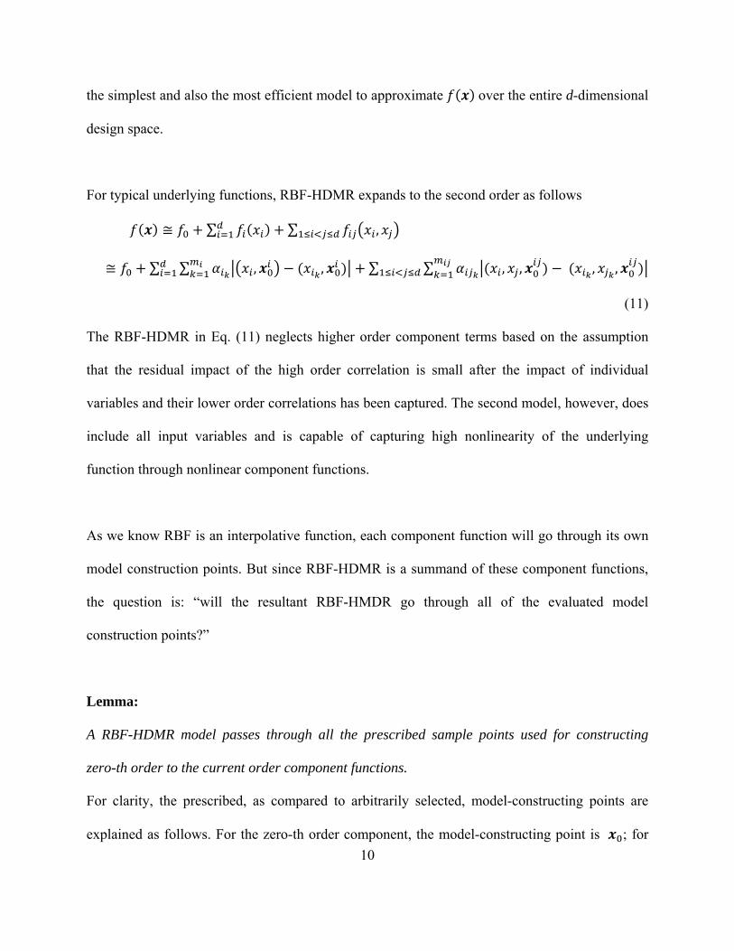
For typical underlying functions, RBF-HDMR expands to the second order as follows

∑ ∑ ,

∑ ∑ , , ∑ ∑ , , , ,

(11)

The RBF-HDMR in Eq. (11) neglects higher order component terms based on the assumption

that the residual impact of the high order correlation is small after the impact of individual

variables and their lower order correlations has been captured. The second model, however, does

include all input variables and is capable of capturing high nonlinearity of the underlying

function through nonlinear component functions.

As we know RBF is an interpolative function, each component function will go through its own

model construction points. But since RBF-HDMR is a summand of these component functions,

the question is: “will the resultant RBF-HMDR go through all of the evaluated model

construction points?”

Lemma:

A RBF-HDMR model passes through all the prescribed sample points used for constructing

zero-th order to the current order component functions.

For clarity, the prescribed, as compared to arbitrarily selected, model-constructing points are

explained as follows. For the zero-th order component, the model-constructing point is ; for

11

the first order components, the model-construction points include and , ; for the

second order components, its model-construction points are , , , , and

, , , .

The lemma is proved as follows. Assuming is the cut center, the RBF-HDMR at first-order is

defined as . Its first order component function is approximated by one

dimensional RBF function ∑ , , by using the function values computed

from , , where is the k-th model-constructing point along xi, and

, is the true function value at point , . Since is a constant and

interpolates all model constructing points, the RBF-HDMR model will interpolate all the

model constructing points and , .

For the second order components, the function values of these components are computed from

, , , , and , is then approximated by a two-

dimensional RBF function ∑ , , , , with points , , ,

, , and , , , . It is easy to see , pass through all the evaluated

points since they all participated in modeling , . For first order component functions,

which are functions of only and orthogonal to each other, they will have zero error at

, , since each goes through . Therefore all first-order component functions,

and therefore the resultant RBF-HDMR model, will pass through all model constructing points

to the second order component function, i.e., , , , , , and , , , .

12

Similarly the RBF-HDMR model passes their model-constructing points till the d-th component.

As the RBF-HDMR has a finite number of terms and each of its component function is exact on

these prescribed model-constructing (or evaluated sample) points, the RBF-HDMR model will

pass through all sample points. The lemma is proved.

The above lemma not only reveals an important feature of RBF-HDMR, it is also a great help to

answer the following question, “if the RBF-HDMR model is built at the l-th order, how to

identify if there is still (l+1)-th order component that need to be modeled?”

Let’s start with l=1, which indicates that all the zero-th and first order component functions have

been modeled using points and , . If the second order component functions are to be

built, we will use the elements in these existing points to create new sample points , ,

for modeling. According to the lemma, the to-be-built second order RBF-HDMR model is then

expected to go through these sample points , , . If the first-order RBF-HDMR model

cannot accurately predict the function value at the new sample point , , , it indicates

that there must exist second order and/or higher order correlation that has not been modeled,

since the approximation error is zero for the first order component functions at points ,

and , ..

To generalize the above discussion, we create a point

, , , , , , , , 0 by random combining the sampled values in

the first order component construction for each input variable (i.e., , di ...,,1= and evaluated at

13

, , respectively). According to the lemma, the complete RBF-HDMR model in Eq. (10)

should interpolate this point, . If an l-th order RBF-HDMR model does not interpolate this

point, it indicates that there is higher order (>l-th) component functions need to be modeled to

decrease the prediction error, and the metamodeling should therefore continue until convergence.

This fact has been incorporated in the metamodeling algorithm, which is to be detailed in Section

4.2.

4. Metamodeling for RBF­HDMR

4.1 Strategies for High Dimensionality

From the recent review [22], the authors find that the cost of modeling an underlying function is

affected by multiple factors including the function’s dimensionality, linearity/nonlinearity,

ranges of input variables, and convergence criteria. Generally speaking, the cost increases as the

dimensionality and nonlinearity rise, the ranges of input variables become larger, and as the

convergence criteria become stricter. This section describes four strategies associated with the

proposed metamodeling method for RBF-HDMR that help to circumvent/alleviate the

computational difficulty brought by the increase of dimensionality without the loss of sampling

resolution.

First, a RBF-HDMR model has a hierarchical structure from zero-th order to d-th order

components. If this structure can be identified progressively, the cost of constructing higher-

order components in HDMR can be saved. The computational cost (i.e. the number of sampling

points) of generating a Cut-HDMR up to the l-th level is given by [15, 16]

14

∑ !! !

1 1 11

2!1 2 1 2

3!1 3

!

1 (12)

Where s is the number of sample points taken for each xi. The cost of Cut-HDMR is related to

the highest order of the Cut-HDMR expansion where the convergence is reached. Each term in

Eq. (12) represents the computational cost for constructing the corresponding order of

component functions. The cost relates to three factors—the dimensionality , the number of

sampling points s for each variable (i.e., take s levels for each variable), and the highest order of

the component functions . The highest order, l, of component functions represents the maximum

number of correlated input variables. As mentioned before, only relatively low-order correlations

of the input variables are expected to have an impact upon the output and high-order correlated

behavior of the input variables is expected to be weak. Typically 3 has been found to be

quite adequate [6]. Considering , a full space resolution 1/s is obtained at the

computational cost less than 1 / 1 !. Thus the exponentially increasing difficulty

is transformed into a polynomial complexity, . This strategy exploits a superposition of

functions of a suitable set of low dimensional variables to represent a high dimensional

underlying function.

Second, for components of the same order, e.g., at the second order with bivariate correlations,

not all possible bivariate correlations may present in the underlying function. Therefore some of

the non-existing correlations among input variables can be identified and eliminated from

modeling to further reduce the cost. The coefficients in Eq. (12), for example, !

, !

,

respectively denote the maximum number of probable combinations of the correlated terms at

15

second and third order component levels. While the number of dimensionality, , cannot be

changed, the number of these coefficients can be reduced if the non-existing correlations can be

identified and eliminated and the modeling cost associated with those terms can therefore be

saved. The developed metamodeling algorithm for RBF-HDMR adaptively identifies such non-

existing correlations and models the underlying function accordingly, which will be described in

the next section.

Third, although the number of sample points, s, for each variable cannot be reduced in order to

keep a certain sampling resolution 1/s, these sample points can be reused for modeling higher-

order component functions. For example, while modeling second-order component functions,

sample points on the reference axes, or hyper-planes, such as , , , and , are re-

used.

Lastly, the number of sample points, s, relates to the degree of the nonlinearity of the underlying

function with respect to the input variable . The higher the degree of the nonlinearity, the more

sample points along are needed to meet the required accuracy. For a linear component, two

sample points are enough to accurately model it. The developed metamodeling algorithm for

RBF-HDMR gradually explores the non-linearity of the component functions and thus

conservatively allocates such cost.

In summary, the RBF-HDMR model naturally helps to transform an exponentially increasing

computational difficulty into a polynomial one by neglecting higher order component functions.

The proposed metamodeling method will also adaptively explore the linearity/nonlinearity of

16

each component function, identify non-existing variable correlations, and reuse sample points to

further reduce the modeling costs.

4.2 Sampling and Model Construction

Based on the proposed RBF-HDMR model, a sampling and model construction algorithm is

developed. The algorithm steps are described as follows:

1. Randomly choose a point , , , in the modeling domain as the cut center.

Evaluating at , we then have .

2. Sample for the first order component functions , , , , , in

the close neighbourhood of the two ends of xi (lower and upper limits) while fixing the rest of xj

(j i) components at . In this work, a neighborhood is defined as one percent of the variable

range which is in the design space and near a designated point. Evaluating these two end points,

we got the left point value , , , , , and the right point value

, , , , , and model the component function as by a

one dimensional RBF model for each variable .

3. Check the linearity of . If the approximation model goes through the center

point, , is considered as linear. In this case, modeling for this component terminates.

Otherwise, use the center point and the two end points to re-construct . Then a random

value along is generated and combined with the rest of xj (j i) components at to form a

new point to test . If is not sufficiently accurate (the relative prediction error is larger

than a given criterion, e.g. 0.1), the test point and all the evaluated points will be used to re-

construct . This sampling-remodeling process iterates till convergence. This process is to

17

capture the nonlinearity of the component function with one sample point at a time. Step 3

repeats for all of the first order component functions to construct the first order terms of RBF-

HDMR model.

4. Form a new point, , , , , , , , , , , 0 by random

combining the sampled value in the first order component construction for each input variable

(i.e., , di ...,,1= and evaluated at , , respectively). This new point is then evaluated by

expensive simulation and the first order RBF-HDMR model. The function values from expensive

simulation and model prediction are compared. If the two values are sufficiently close (the

relative error is less than a small value, e.g. 0.1), it indicates that no higher-order terms exist in

the underlying function, the modeling process terminates. Otherwise, go to the next Step.

5. Use the values of and , that exist in thus-far evaluated points ,

, , , , , , and , , , , , , to form new points of the

form , , , , , , , , , . Randomly select one of the points from

these new points to test the first-order RBF-HDMR model. If the model passes through the new

point, it indicates that xi and xj are not correlated and the process continues with the next pair of

input variables. This is to save the cost of modeling non-existing or insignificant correlations.

Otherwise, use this new point and the evaluated points , and , to construct the

second order component function, , . This sampling-remodeling process iterates for all

possible two-variable correlations until convergence (e.g., the relative prediction error is less

than 0.1). Step 5 is repeated for all pairs of input variables.

18

Theoretically, Step 5 applies to all higher-order terms in RBF-HDMR model, Eq. (10), in a

similar manner. In this work, the process proceeds towards the end of the second order terms

based on the Premise 2 in the introduction section. The identification of correlations in Steps 4

and 5 is supported by the discussions in Section 3.

4.3 An Example for Metamodeling RBF-HDMR

For the ease of understanding, consider the following mathematical function with d = 3

4, 0 1 (13)

Table 1 shows the modeling processes – finding , modeling the first order components

, 1, ,3, detecting and exploiting linearity and correlation relationship in the

underlying function, and modeling higher order components, , , if they exist. This process

continues until convergence. The first and last rows list the original function and the

corresponding RBF-HDMR model, respectively. Each middle row demonstrates the modeling

process in hierarchy. The detailed steps are as follows.

Step 1. Randomly sample the cut center in the neighbourhood of the center of the design

space, in this case, 0.5, 0.5, 0.5 and then find .

Step 2. Randomly sample at its two ends, and form two new points , (one per end) and

evaluate them. Model the component functions using the two end points. For example, for x1,

two values 0 and 1 are sampled; we can use the function values [f (0, 0.5, 0.5)-f0] and [f (1, 0.5,

0.5)-f0] as their function values for 0 and 1, respectively to model f1(x1). Note that the special

19

RBF format as in the Appendix is used rather than the simple linear spline format to avoid matrix

singularity.

Step 3. Detect the linearity of the output function with respect to each variable by comparing

and . If nonlinearity exists, model , 1, ,3 till convergence. The f2(x2)

component function, for instance, is a nonlinear function. In addition to the two end points 0 and

1, two more new sample points are generated at 0.19 and 0.81 to capture its nonlinearity. All of

the component functions are plotted with a distance in the last column in Table 1.

Step 4. Identify if correlation exists. If no, terminate modeling. Otherwise, go to Step 5. In this

case, since there exists correlation between x1 and x3, the modeling process continues.

Step 5. Identify the correlated terms according to Step 5 of the algorithm described in Section 4.2.

If correlation exists in the underlying function, model the identified correlated terms. In this case,

only the correlated term exists, which needs to be modeled as a component function. Repeat

Step 5 until convergence.

To better understand Table 1, let us take modeling as an example. When

modeling , five values along are generated, i.e., 0, 1, 0.5, 0.19, 0.81, according to the

sampling algorithm described in Section 4.2. By combining these values with other

component values except for , we have five new points and their function values are evaluated.

Deducted the value from their function values, we obtain the component function

values for these five points are, respectively, -0.25, 0.75, 0.0, -0.2139, 0.4061. Employing these

five points and their function values to fit the RBF function as defined in the Appendix, one can

have the RBF model for , with five nonlinear terms and two polynomial terms, as shown

in the last row of Table 1.

20

In Table 1, is especially noteworthy. One can see from the original function expression

that there is no separate x3 term in the function, but an x1x3 term. Why is not zero? This

is because HDMR first finds the first order influence of , the residual then goes to the second

order component function , . Therefore, it would be wrong to mechanically match the

component functions with the terms in the underlying function. As a matter of fact, the x1x3 term

in the original function has been expressed by and , , as well as partially by

.

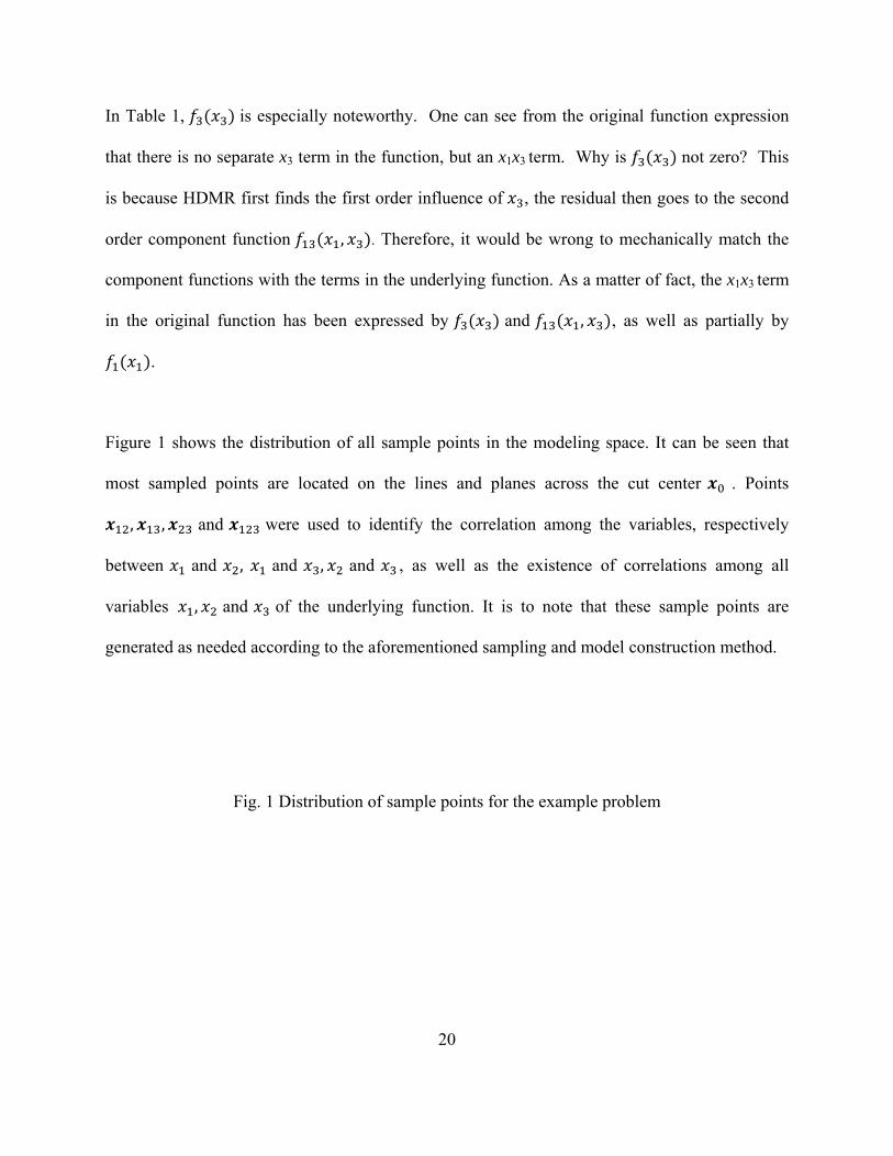
Figure 1 shows the distribution of all sample points in the modeling space. It can be seen that

most sampled points are located on the lines and planes across the cut center . Points

, , and were used to identify the correlation among the variables, respectively

between and , and , and , as well as the existence of correlations among all

variables , and of the underlying function. It is to note that these sample points are

generated as needed according to the aforementioned sampling and model construction method.

Fig. 1 Distribution of sample points for the example problem

21

Table 1 Process of modeling RBF-HDMR for the example problem

Function 4, 0 1 0.5, 0.5, 0.5 3

Linearity Samples ix Observed 0),( fxxf i

i − RBF coefs

Component Function Plot

(linear)

0 1 0.5

-3.75 -2.25 -3

-0.75 0.75 0

0 0 0 -0.75 1.5

(non-linear)

0 1 0.5 0.19 0.81

-3.25 -2.25 -3 -3.2139 -2.5939

-0.25 0.75 0 -0.2139 0.4061

0.6796 0.6796 -0.1754 -0.5918 -0.5918 -0.3977 1

(linear)

0 1 0.5

-3.25 -2.75 -3

-0.25 0.25 0

0 0 0 -0.25 0.5

,

Correlation Relationship Sampling

, Observed

, ,

RBF coefs

, null null null null

,

(0.5,0.5); (0,0.5); (1,0.5); (0.5,0); (0.5, 1); (0,0); (1,1); (0,1); (1,0);

-3 -3.75 -2.25 -3.25 -2.75 -3.75 -1.75 -3.75 -2.75

0 0 0 0 0 0.25 0.25 -0.25 -0.25

0;0;0;0;0; 0.3607; 0.3607; -0.3607; -0.3607; 0;0;0

, null null null null

30

0.75 1.51

0.6796| | log| | 0.6796| 1| log| 1| 0.1754| 0.5| log| 0.5| 0.5918| 0.19| log| 0.19| 0.5918| 0.81| log| 0.81| 0.39772

0.25 0.5

0.3607 log 0.3607 11 log 1

1 0.3607 01 log 0

1 0.3607 10 log 1

0

0 0.5 1

-2.5

-3

-3.5

0 0.5 1

-2

-3

-4

0 0.5 1

-2

-3

-4

22

Given the metamodel as expressed in the last row of Table 1, one can observe that all first order

functions are linear except for f2, which indicates that x2 has a nonlinear influence to the overall f

function while others have linear effects. For the second order components, only a nonlinear f13

is present, indicating other variables are not correlated.

5. Testing of RBF-HDMR

Problems from literature are used for testing the proposed RBF-HDMR and its metamodeling

method. The modeling efficiency is indicated by the number of (expensive) sample points. The

modeling accuracy is evaluated by three performance metrics. A comparison of the RBF-HDMR

model with other metamodels is also given.

5.1 Performance Metrics

There are various commonly-used performance metrics for approximation models that are given

in [22]. To the authors’ knowledge, however, there are no specially defined performance metrics

for high dimensional approximation models in the open literature. In mathematics, where the

high dimensional problems are mostly (and yet not adequately) studied, the percentage relative

error is often used as a metric for model validation. It is found, however, when the absolute

errors of the metamodels are quite small, their percentage relative errors could be extremely

large when the function value is close to zero. The percentage relative error measure is also

dependent on the problem scale, which makes the comparison between problems disputable. In

the engineering design, the cross-validation method is currently a popular method for model

validation. However, Lin [23] found that the cross-validation is an insufficient measurement for

metamodel accuracy. The cross-validation is actually a measurement for degrees of insensitivity

23

of a metamodel to lost information at its data points, while an insensitive metamodel is not

necessarily accurate. To be consistent with Ref. [5], which will be used for result comparison,

this work employs three commonly used performance metrics —R square, relative average

absolute error (RAAE) and relative maximum absolute error (RMAE) —for validating

approximation models. After the RBF-HDMR modeling process is terminated, additional 10,000

new random sample points are used to evaluate the model against the three performance metrics

by Monte Carlo simulation. The values of these performance metrics show the prediction

capability of the RBF-HDMR on new points. It is to be noted that these three metrics all need a

fairly large number of validation points to be meaningful but for High dimensional, Expensive,

Black-box (HEB) problems such information are too costly to obtain. This is in contrast to high

dimensional problems studied in mathematics where those are inexpensive problems and a large

quantity of validation points is affordable. Validation methodology for HEB problems is

therefore worth further research. Since this work also chose mathematical problems for testing

and comparison, we can still employ the three metrics with Monte Carlo simulations for

validation. These metrics are described as below:

1) R Square:

1 ∑∑ (14)

Where denotes the mean of function on m sample points. This metrics indicates the overall

accuracy of an approximation model. The closer the value of R square approaches one, the more

accurate is the approximation model. Note that R2 is evaluated on the new validation points, not

on the modeling points. The same is true for RAAE and RMAE.

2) Relative Average Absolute Error (RAAE):

24

∑ | | (15)

where STD stands for standard deviation. Like R square, this metric shows the overall accuracy

of an approximation model. The closer the value of RAAE approaches zero, the more accurate is

the approximation model.

3) Relative Maximum Absolute Error (RMAE):

, , , (16)

This is a local metric. A RMAE describes error in a sub-region of the design space. Therefore, a

small value of RMAE is preferred.

5.2 Study Problem

A problem for large-scale optimization in MatlabTM optimization toolbox is chosen to study the

performance of RBF-HDMR and its metamodeling method as a function of the dimensionality,

d.

∑ , 0 1 (17)

This highly nonlinear problem was tested with d=30, 50, 100, 150, 200, 250 and 300. For each d,

ten runs have been taken and the mean values of R square, RAAE and RMAE are charted in Fig.

3.

Fig. 2 Performance metrics mean with respect to d (x-axis) for the study problem

As seen from Fig. 2, although the three accuracy performance metrics deteriorate slightly as d

increases, they demonstrate that the RBF-HDMR model fits well the high dimensional

25

underlying function. The minimum (worst) value of R square is close to 0.9, the maximum

(worst) values of RAAE is about 0.32 and the maximum (worst) value of RMAE is about 0.54.

The data explains the RBF-HDMR model has a good fit of the underlying function.

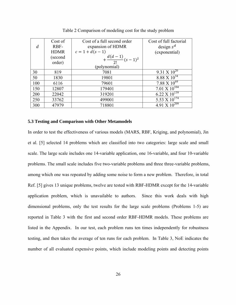
Regarding to modeling cost, assuming five samples are taken along each axes (s = 5), we list the

number of evaluations for RBF-HDMR model, full second order expansion of the HDMR

(polynomially increasing cost), and the full factorial design of experiments (exponentially

increasing cost) for various dimensionality d in Table 2. The comparison clearly shows the

computational advantage of the proposed RBF-HDMR. The efficiency of the proposed method

will be further studied in comparison with Latin Hypercube samples in the next section.

26

Table 2 Comparison of modeling cost for the study problem

d

Cost of RBF-

HDMR (second order)

Cost of a full second order expansion of HDMR

1 11

2!1

(polynomial)

Cost of full factorial design

(exponential)

30 819 7081 9.31 X 1020

50 1830 19801 8.88 X 1034

100 6116 79601 7.88 X 1069

150 12807 179401 7.01 X 10104

200 22042 319201 6.22 X 10139

250 33762 499001 5.53 X 10174

300 47979 718801 4.91 X 10209

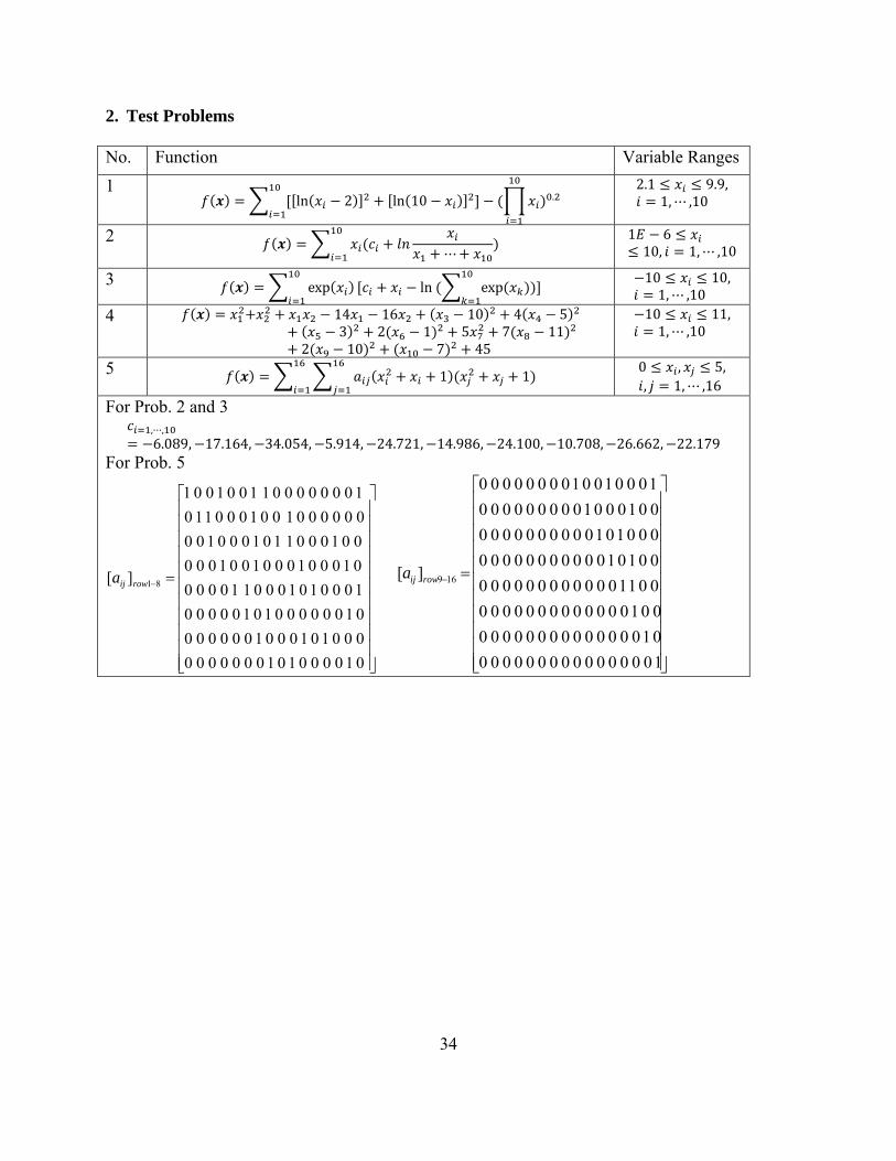
5.3 Testing and Comparison with Other Metamodels

In order to test the effectiveness of various models (MARS, RBF, Kriging, and polynomial), Jin

et al. [5] selected 14 problems which are classified into two categories: large scale and small

scale. The large scale includes one 14-variable application, one 16-variable, and four 10-variable

problems. The small scale includes five two-variable problems and three three-variable problems,

among which one was repeated by adding some noise to form a new problem. Therefore, in total

Ref. [5] gives 13 unique problems, twelve are tested with RBF-HDMR except for the 14-variable

application problem, which is unavailable to authors. Since this work deals with high

dimensional problems, only the test results for the large scale problems (Problems 1-5) are

reported in Table 3 with the first and second order RBF-HDMR models. These problems are

listed in the Appendix. In our test, each problem runs ten times independently for robustness

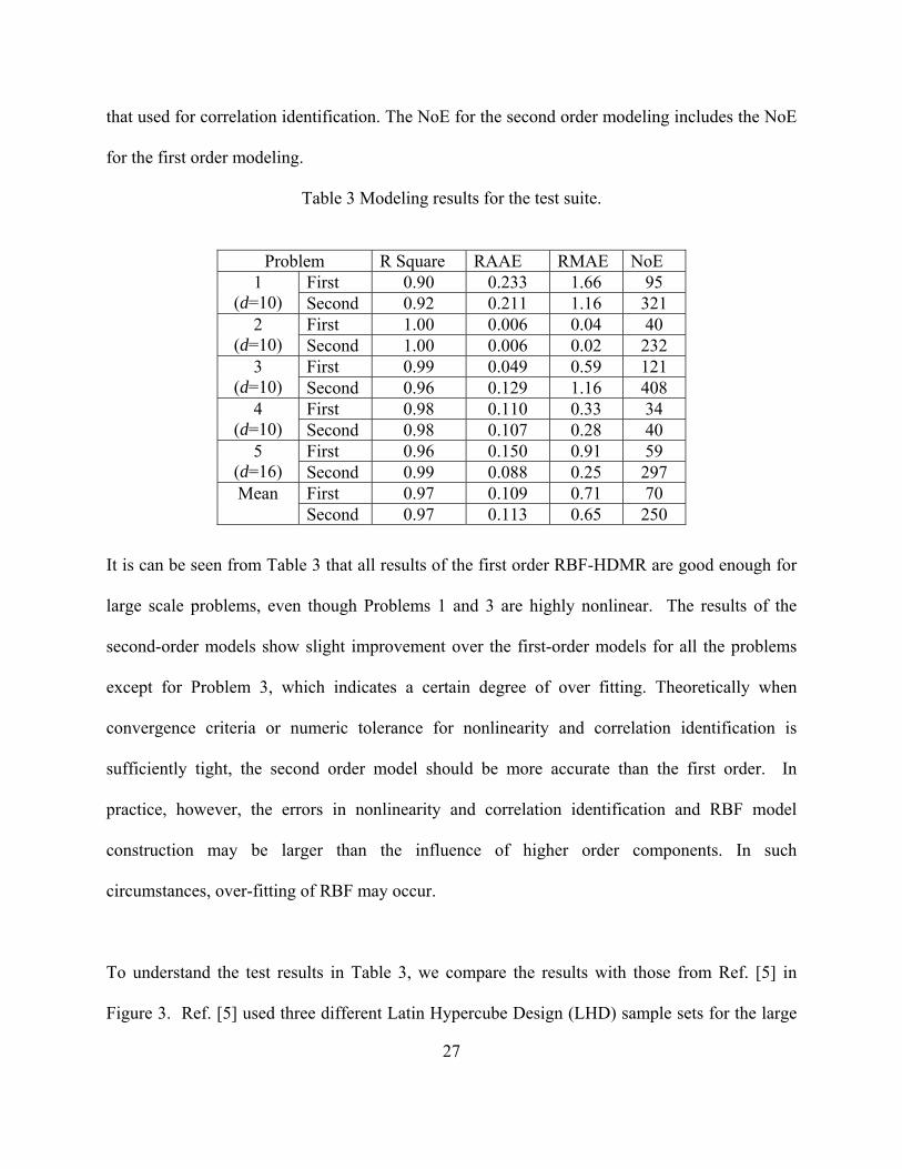
testing, and then takes the average of ten runs for each problem. In Table 3, NoE indicates the

number of all evaluated expensive points, which include modeling points and detecting points

27

that used for correlation identification. The NoE for the second order modeling includes the NoE

for the first order modeling.

Table 3 Modeling results for the test suite.

It is can be seen from Table 3 that all results of the first order RBF-HDMR are good enough for

large scale problems, even though Problems 1 and 3 are highly nonlinear. The results of the

second-order models show slight improvement over the first-order models for all the problems

except for Problem 3, which indicates a certain degree of over fitting. Theoretically when

convergence criteria or numeric tolerance for nonlinearity and correlation identification is

sufficiently tight, the second order model should be more accurate than the first order. In

practice, however, the errors in nonlinearity and correlation identification and RBF model

construction may be larger than the influence of higher order components. In such

circumstances, over-fitting of RBF may occur.

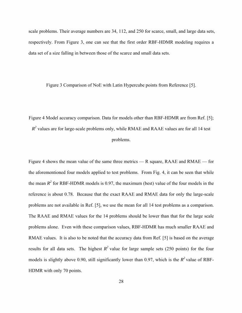
To understand the test results in Table 3, we compare the results with those from Ref. [5] in

Figure 3. Ref. [5] used three different Latin Hypercube Design (LHD) sample sets for the large

Problem R Square RAAE RMAE NoE 1

(d=10) First 0.90 0.233 1.66 95 Second 0.92 0.211 1.16 321

2 (d=10)

First 1.00 0.006 0.04 40 Second 1.00 0.006 0.02 232

3 (d=10)

First 0.99 0.049 0.59 121 Second 0.96 0.129 1.16 408

4 (d=10)

First 0.98 0.110 0.33 34 Second 0.98 0.107 0.28 40

5 (d=16)

First 0.96 0.150 0.91 59 Second 0.99 0.088 0.25 297

Mean First 0.97 0.109 0.71 70 Second 0.97 0.113 0.65 250

28

scale problems. Their average numbers are 34, 112, and 250 for scarce, small, and large data sets,

respectively. From Figure 3, one can see that the first order RBF-HDMR modeling requires a

data set of a size falling in between those of the scarce and small data sets.

Figure 3 Comparison of NoE with Latin Hypercube points from Reference [5].

Figure 4 Model accuracy comparison. Data for models other than RBF-HDMR are from Ref. [5];

R2 values are for large-scale problems only, while RMAE and RAAE values are for all 14 test

problems.

Figure 4 shows the mean value of the same three metrics — R square, RAAE and RMAE — for

the aforementioned four models applied to test problems. From Fig. 4, it can be seen that while

the mean R2 for RBF-HDMR models is 0.97, the maximum (best) value of the four models in the

reference is about 0.78. Because that the exact RAAE and RMAE data for only the large-scale

problems are not available in Ref. [5], we use the mean for all 14 test problems as a comparison.

The RAAE and RMAE values for the 14 problems should be lower than that for the large scale

problems alone. Even with these comparison values, RBF-HDMR has much smaller RAAE and

RMAE values. It is also to be noted that the accuracy data from Ref. [5] is based on the average

results for all data sets. The highest R2 value for large sample sets (250 points) for the four

models is slightly above 0.90, still significantly lower than 0.97, which is the R2 value of RBF-

HDMR with only 70 points.

29

In summary, from the comparison with the reference, the proposed RBF-HDMR model and its

metamodeling method generates more accurate models with fewer sample points than

conventional models such as MARS, RBF, Kriging, and polynomial functions with Latin

Hypercube designs.

5.4 Discussion

This work employs RBF to model component functions of the HDMR, so that HDMR is no

longer a check-up table but rather a complete equation. The proposed metamodeling approach

takes advantages of properties of HDMR to make the sampling efficient. RBF was chosen

because of 1) its simplicity and robustness in model construction 2) the ease of obtaining an

explicit function expression, and 3) its ability to interpolate the sample points (this could be a

problem for noisy data, which will be a topic of our future research). The integration of HDMR

with the interpolative feature of RBF supports the developed lemma and the sampling method,

especially on identification of nonlinearity, variable correlations, and higher order components.

Therefore RBF helps to reduce the sample size. The choice of a specific RBF form, as shown in

the Appendix, is deliberate as it is better than a simple linear spline for avoiding singularity.

Exploration of other interpolative metamodels and selection of the best metamodel for

component functions may be a topic for future research.

The proposed metamodeling approach takes advantage of the hierarchical structure of HDMR,

adaptively models its component functions while exploring its inherent linearity/nonlinearity and

correlation among variables. The sample points are thus limited and well controlled. The realized

30

samples spread in the design space (refer to Fig. 1), but unevenly, according to complexity of

regions in the space. Regions of high nonlinearity or correlation will have more sample points

while linear regions have fewer points, all according to the needs to capture the behavior of the

underlying function. In contrast, the Latin Hypercube Design (LHD) has only one-dimensional

uniformity and it is “blind” to the function characteristics. It is also worth noting that the

metamodeling process only involves fast and simple algebraic operations, which also lends itself

well for parallel computation at each order of component levels. The outputs are multitude, i.e.,

an explicit RBF-HDMR model, function linearity/non-linearity, correlations among variables,

and so on.

The RBF-HDMR at currently stage, however, only models to the second-order components. If

an underlying function has significant multivariate correlation, the method may be limited. New

approaches are needed to extend beyond the second-order, whereas keeping the modeling cost

low. Secondly, the proposed RBF-HDMR adaptively determines the location of sample points,

which is attractive when there is no existing data and the goal is to reduce the number of function

evaluations. In real practice, however, there are situations that some expensive data may have

already been generated. Strategies needed to be developed to take advantage of the existing data

when constructing RBF-HDMR. Thirdly, RBF-HDMR at its current stage only deals with

deterministic problems while in practice the expensive model may be noisy. Future research is

needed to deal with these issues.

6. Conclusion

31

This work proposes a methodology of metamodeling High dimensional, Expensive, and Black-

box (HEB) problems. The methodology consists of the proposed RBF-HDMR metamodel, and

its accompanying metamodeling method. The RBF-HDMR model inherits hierarchical structural

properties of HDMR, provides an explicit expression with RBF components, and needs neither

any knowledge about the underlying functions nor assumes a priori a parametric form. The

modeling process automatically explores and makes use of the properties of the underlying

functions, refines the model accuracy by iterative sampling in the subspace of nonlinearity and

correlated variables, and involves only fast and simple algebraic operations that can be easily

parallelized. The developed methodology alleviates or circumvents the “curse of dimensionality.”

Testing and comparison with other metamodels reveal that RBF-HDMR models high

dimensional problems with higher efficiency and accuracy. Future research aims to extend the

modeling approach to efficiently model high-order components, to use existing data, and to deal

with noisy samples.

Acknowledgment

Funding supports from Canada Graduate Scholarships (CGS) and Natural Science and

Engineering Research Council (NSERC) of Canada are gratefully acknowledged.

Appendix

1. RBF model

A general radial basis functions (RBF) model [2,5] is shown as follows.

∑ | | (A.1)

32

Where iβ is the coefficient of the expression and are the sampled points of input variables or

the centers of RBF approximation. . is a distance function or the radial basis function. .

denotes a p-norm distance. A RBF is a real-valued function whose value depends only on the

distance from center points . It employs linear combinations of a radically symmetric function

based on the distance to approximate underlying functions. Its advantages include: the number of

sampled points for constructing approximation can be small and the approximations are good fits

to arbitrary contours of response functions [2]. Consequently, RBF is a popular model for

multivariate data interpolation and function approximations.

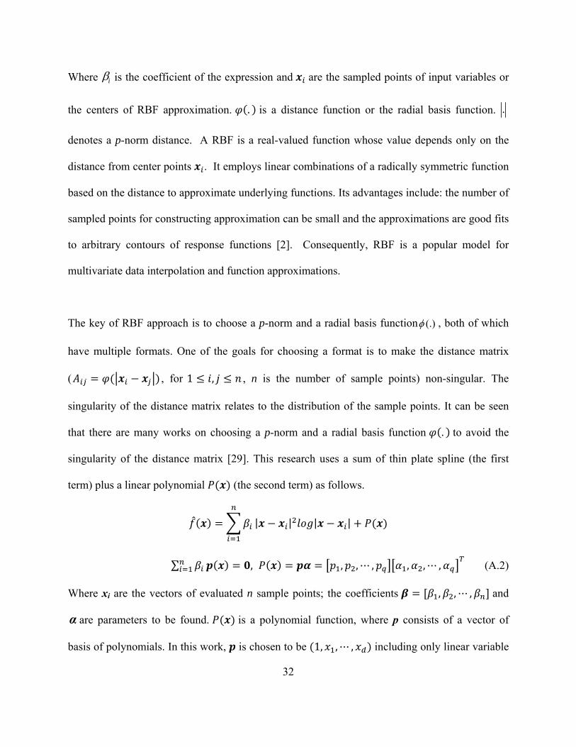
The key of RBF approach is to choose a p-norm and a radial basis function (.)φ , both of which

have multiple formats. One of the goals for choosing a format is to make the distance matrix

( , for 1 , , n is the number of sample points) non-singular. The

singularity of the distance matrix relates to the distribution of the sample points. It can be seen

that there are many works on choosing a p-norm and a radial basis function . to avoid the

singularity of the distance matrix [29]. This research uses a sum of thin plate spline (the first

term) plus a linear polynomial (the second term) as follows.

| | | |

∑ , , , , , , , (A.2)

Where xi are the vectors of evaluated n sample points; the coefficients , , , and

α are parameters to be found. is a polynomial function, where p consists of a vector of

basis of polynomials. In this work, is chosen to be 1, , , including only linear variable

33

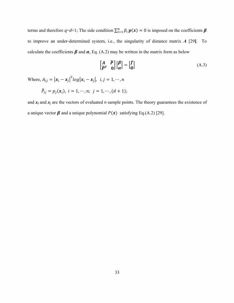
terms and therefore q=d+1; The side condition ∑ 0 is imposed on the coefficients

to improve an under-determined system, i.e., the singularity of distance matrix A [29]. To

calculate the coefficients and , Eq. (A.2) may be written in the matrix form as below

(A.3)

Where, , , 1, ,

, 1, , ; 1, , 1 ;

and xi and xj are the vectors of evaluated n sample points. The theory guarantees the existence of

a unique vector and a unique polynomial satisfying Eq.(A.2) [29].

34

2. Test Problems

No. Function Variable Ranges 1

ln 2 ln 10 .2.1 9.9,

1, ,10

2 1 610, 1, ,10

3 exp ln exp 10 10,

1, ,10 4 14 16 10 4 5

3 2 1 5 7 112 10 7 45

10 11,1, ,10

5 1 1 0 , 5,, 1, ,16

For Prob. 2 and 3 , ,6.089, 17.164, 34.054, 5.914, 24.721, 14.986, 24.100, 10.708, 26.662, 22.179

For Prob. 5

⎥⎥⎥⎥⎥⎥⎥⎥⎥⎥⎥

⎦

⎤

⎢⎢⎢⎢⎢⎢⎢⎢⎢⎢⎢

⎣

⎡

=−

01000010100000000001010001000000010000001010000010001010001100000100010001001000001000110100010000000010010001101000000011001001

][ 81rowija

⎥⎥⎥⎥⎥⎥⎥⎥⎥⎥⎥

⎦

⎤

⎢⎢⎢⎢⎢⎢⎢⎢⎢⎢⎢

⎣

⎡

=−

10000000000000000100000000000000001000000000000000110000000000000010100000000000000101000000000000100010000000001000100100000000

][ 169rowija

35

References

[1] Wang, G. G. and Shan, S., 2007, "Review of Metamodeling Techniques in Support of Engineering Design Optimization," Transactions of the ASME, Journal of Mechanical Design, 129, pp. 370-389.

[2] Chen, V., C. P., Tsui, K.-L., Barton, R. R. and Meckesheimer, M., 2006, "A Review on Design, Modeling and Applications of Computer Experiments," IIE Transactions, 38, pp. 273-291.

[3] Simpson, T. W., Toropov, V., Balabanov, V., Viana, F. A. C., "Design and Analysis of Computer Experiments in Multidisciplinary Design Optimization: A Review of How Far We Have Come – or Not," 12th AIAA/ISSMO Multidisciplinary Analysis and Optimization Conference 10 - 12 September 2008, Victoria, British Columbia Canada, AIAA 2008-5802.

[4] Welch, W. J., Buck, R. J., Sacks, J., Wynn, H. P., Mitchell, T. J. and Morris, M. D., 1992, "Screening, Predicting, and Computer Experiments," Technometrics, 34(1), pp. 15-25.

[5] Jin, R., Chen, W. and Simpson, T. W., 2001, "Comparative Studies of Metamodeling Techniques under Multiple Modeling Criteria," Structural and Multidisciplinary Optimization, 23(1), pp. 1-13.

[6] Shorter, J. A., Ip, P. C. and Rabitz, H. A., 1999, "An Efficient Chemical Kinetics Solver Using High Dimensional Model Representation," Journal of Physical Chemistry A, (103), pp. 7192-7198.

[7] Bates, R. A., Buck, R. J., Riccomagno, E. and Wynn, H. P., 1996, "Experimental Design and Observation for Large Systems," Journal of the Royal Statistical Society: B, 58(1), pp. 77-94.

[8] Booker, A. J., Dennis, J. E. J., Frank, P. D., Serafini, D. B., Torczon, V. and Trosset, M. W., 1999, "A Rigorous Framework for Optimization of Expensive Functions by Surrogates," Structural Optimization, 17(1), pp. 1-13.

[9] Koch, P. N., Simpson, T. W., Allen, J. K. and Mistree, F., 1999, "Statistical Approximations for Multidisciplinary Design Optimization: The Problem of Size," Journal of Aircraft, 36(1), pp. 275-286.

[10] Tu, J. and Jones, D. R., 2003, "Variable Screening in Metamodel Design by Cross-Validated Moving Least Squares Method," 44th AIAA/ASME/ASCE/AHS Structures, Structural Dynamics, and Materials Conference Norfolk, Virginia, April 7-10.

[11] Friedman, J. H. and Stuetzle, W., 1981, "Projection Pursuit Regression," Journal of the American Statistical Association, 76(372), pp. 817-823.

[12] Friedman, J. H., 1991, "Multivariate Adaptive Regressive Splines," The Annals of Statistics, 19(1), pp. 1-67.

[13] Sobol, I. M., 1993, "Sensitivity Estimates for Nonlinear Mathematical Models," Mathematical Modeling & Computational Experiment, 1(4), pp. 407-414.

[14] Li, G., Wang, S.-W., Rosenthal, C. and Rabitz, H., 2001, "High Dimensional Model Representations Generated from Low Dimensional Data Samples. I. Mp-Cut-HDMR," Journal of Mathematical Chemistry, 30(1), pp. 1-30.

[15] Rabitz, H. and Al1s, Ö. F., 1999, "General Foundations of High-Dimensional Model Representations," Journal of Mathematical Chemistry (25), pp. 197-233.

[16] Li, G., Rosenthal, C. and Rabitz, H., 2001, "High Dimensional Model Representations," Journal of Physical Chemistry A, 105(33), pp. 7765-7777.

[17] Li, G., Hu, J., Wang, S.-W., Georgopoulos, P. G., Schoendorf, J. and Rabitz, H., 2006, "Random Sampling-High Dimensional Model Representation (Rs-HDMR) and Orthogonality of Its Different Order Component Functions," Journal of Physical Chemistry A, (110), pp. 2474-2485.

[18] Wang, S.-W., Georgopoulos, P. G., Li, G. and Rabits, H., 2003, "Random Sampling-High Dimensional Model Representation (RS-HDMR) with Nonuniformly Distributed Variables: Application to an Integrated Multimedia/Multipathway Exposure and Dose Model for Trichloroethylene," Journal of Physical Chemistry A, (107), pp. 4707-4716.

[19] Tunga, M. A. and Demiralp, M., 2005, "A Factorized High Dimensional Model Representation on the Nodes of a Finite Hyperprismatic Regular Grid," Applied Mathematics and Computation (164), pp. 865-883.

[20] Tunga, M. A. and Demiralp, M., 2006, "Hybrid High Dimensional Model Representation (HDMR) on the Partitioned Data," Journal of Computational and Applied Mathematics, (185), pp. 107-132.

[21] Sobol, I.M., 2003, “Theorems and examples on high dimensional model representation,” Reliability Engineering and System Safety 79, pp. 187–193.

36

[22] Shan, S. and Wang, G. G., 2010, "Survey of Modeling and Optimization Strategies to Solve High-Dimensional Design Problems with Computationally-Expensive Black-Box Functions," Structural and Multidisciplinary Optimization, 41(2), pp. 219-241 DOI: 10.1007/s00158-009-0420-2.

[23] Lin, Y., 2004, "An Efficient Robust Concept Exploration Method and Sequential Exploratory Experimental Design," Mechanical Engineering, Georgia Institute of Technology, Atlanta, Ph. D. Thesis.

[24] Jin, R., Chen, W. and Sudjianto, A., 2005, "An Efficient Algorithm for Constructing Optimal Design of Computer Experiments," Journal of Statistical Planning and Inferences, 134(1), pp. 268-287.

[25] Sasena, M., Parkinson, M., Goovaerts, P., Papalambros, P. and Reed, M., 2002, "Adaptive Experimental Design Applied to an Ergonomics Testing Procedure," ASME 2002 Design Engineering Technical Conferences and Computer and Information in Engineering Conference, ASME, Montreal, Canada.

[26] Wang, G. G., 2003, "Adaptive Response Surface Method Using Inherited Latin Hypercube Design Points," Transactions of the ASME, Journal of Mechanical Design, 125, pp. 210-220.

[27] Jin, R., Chen, W. and Sudjianto, A., 2002, "On Sequential Sampling for Global Metamodeling in Engineering Design," ASME 2002 Design Engineering Technical Conferences and Computer and Information in Engineering Conference, Montreal, Canada.

[28] Owen, A. B., 2000, "Assessing Linearity in High Dimensions," The Annals of Statistics, 28(1), pp. 1-19. [29] Baxter, B. J. C., 1992, "The Interpolation Theory of Radial Basis Functions," Trinity College, Cambride

Univeristy, Ph. D. Thesis.