©20

12 N

atur

e A

mer

ica,

Inc.

All

righ

ts r

eser

ved.

PROTOCOL

508 | VOL.7 NO.3 | 2012 | NATURE PROTOCOLS

INTRODUCTIONMetabolites are the biochemical end products of gene activity, and they therefore provide a functional readout of cellular phenotype1–3. Untargeted metabolomics is the global and simultaneous profiling of as many metabolites as possible in a search to identify altered pathways that provide a phenotypic signature for the biological system of interest4–7. The approach has been widely applied to elu-cidate biomarkers of disease, to discover new therapeutic targets, to assign unknown gene function and to gain mechanistic insight into physiological processes in plants, yeast, bacteria and mammals8–13. Although historically much attention has been dedicated to the analysis of metabolites, until recently most studies focused on a relatively small number of compounds. However, developments in high-resolution mass spectrometers now enable the simultane-ous detection of thousands of low-concentration species and have largely driven the field of global metabolic profiling over the course of the past 10 years14,15.

As with any ‘omics’ technology, the development of metabolomics has relied on advances in bioinformatic tools that are required for analysis of the complex data sets generated. The analytical tech-nique that has proven to be the most suitable for looking at the largest number of compounds is liquid chromatography/mass spectrometry (LC/MS)14,16. A typical LC/MS analysis of a meta-bolic extract from a biological tissue or fluid results in the detec-tion of thousands of peaks, each characterized by a unique m/z value and/or retention time17,18. The first bioinformatic challenge in LC/MS-based metabolomics was comparing the intensity of individual peaks, known as metabolite features, across all of the samples measured. A complication is that the retention time of a particular metabolite can change slightly from one run to the next due to experimental drift. Deviations in retention time (e.g., from fluctuations in the room temperature, time-dependent changes in the sample and column degradation) are nonlinear and compli-cate the feature assignments that are used for correlation between samples19. In 2005, a metabolomic program was developed called

XCMS, which was used to identify dysregulated metabolite features between two sample groups by using a novel nonlinear retention- time alignment algorithm that does not require the addition of internal standards17. XCMS is a freely available and platform- independent R package that processes, analyzes and visualizes LC/MS metabolomic data. XCMS is widely used in the field of untargeted metabolomics, with over 350 citations of the original paper and more than 45,000 downloads as of 2011.

Although XCMS and other metabolomic programs that have been developed are well suited for the analysis of large sample numbers, the programs are limited in that they only compare two different sample groups directly20,21. Manual comparisons of multiple sets of XCMS results have been performed, but these studies involve only a small number of sample groups and require additional analysis time22. metaXCMS was developed to provide a tool for efficient meta-analysis of untargeted metabolomic data sets containing any number of sample groups23. Meta-analysis can be defined as an approach that compares the results from two or more independently performed studies to identify data points that are unique or shared among all or some of the experimental groups24. Figure 1 highlights the application of metaXCMS to identify unique and shared metabolite features that are dysregulated between three independent pairwise comparisons. Similar types of meta-analysis tools have been suc-cessfully applied in genome-wide association studies to investigate conditions with complex and heterogeneous phenotypes25–27.

ApplicationsTo drive our understanding of chemical physiology, dysregulated metabolites and related cellular pathways need to be specifically correlated with unique biological processes or disease states. Often, however, an untargeted metabolomic analysis results in a substantial number of altered metabolite features and it is a major challenge to differentiate molecules that are causally associated with the pheno-type of interest from those that are altered as a downstream effect.

Meta-analysis of untargeted metabolomic data from multiple profiling experimentsGary J Patti1–3,5, Ralf Tautenhahn4,5 & Gary Siuzdak4

1Department of Genetics, Washington University School of Medicine, St. Louis, Missouri, USA. 2Department of Chemistry, Washington University School of Medicine, St. Louis, Missouri, USA. 3Department of Medicine, Washington University School of Medicine, St. Louis, Missouri, USA. 4Department of Chemistry and Molecular Biology, Center for Metabolomics, Scripps Research Institute, La Jolla, California, USA. 5These authors contributed equally to this work. Correspondence should be addressed to G.S. (siuzdak@scripps.edu).

Published online 16 February 2012; doi:10.1038/nprot.2011.454

metaXCMS is a software program for the analysis of liquid chromatography/mass spectrometry–based untargeted metabolomic data. It is designed to identify the differences between metabolic profiles across multiple sample groups (e.g., ‘healthy’ versus ‘active disease’ versus ‘inactive disease’). Although performing pairwise comparisons alone can provide physiologically relevant data, these experiments often result in hundreds of differences, and comparison with additional biologically meaningful sample groups can allow for substantial data reduction. By performing second-order (meta-) analysis, metaXCMS facilitates the prioritization of interesting metabolite features from large untargeted metabolomic data sets before the rate-limiting step of structural identification. Here we provide a detailed step-by-step protocol for going from raw mass spectrometry data to metaXCMS results, visualized as Venn diagrams and exported Microsoft Excel spreadsheets. There is no upper limit to the number of sample groups or individual samples that can be compared with the software, and data from most commercial mass spectrometers are supported. The speed of the analysis depends on computational resources and data volume, but will generally be less than 1 d for most users. metaXCMS is freely available at http://metlin.scripps.edu/metaxcms/.

©20

12 N

atur

e A

mer

ica,

Inc.

All

righ

ts r

eser

ved.

PROTOCOL

NATURE PROTOCOLS | VOL.7 NO.3 | 2012 | 509

Here metaXCMS provides a broadly applicable data-reduction strat-egy, as we recently showed in a study of three different mouse mod-els of pain that were characterized by unique pathogenic etiology (Fig. 2)23. Mice injected with complete Freund’s adjuvant were used as an inflammatory model, those to which noxious heat was acutely applied to the hind paw were used as an acute heat model and mice that were intraperitoneally injected with serum from K/BxN mice were used as a pain model of spontaneous arthritis28–30. Although the pairwise comparisons of each pain model with its respective control resulted in hundreds of altered metabolite features in total, we suspected that at least some of these molecules may be involved in triggering the transduction of pain signals. The second-order analysis of the results with metaXCMS showed that only three of the altered molecules were shared among all of the models. We deter-mined that one of the shared differences was the well-characterized pain mediator histamine, thereby validating the value of the meta-analysis for identifying mechanistically relevant metabolites causally associated with the phenotype of interest. A comparable approach could be applied to any type of disease or stress model.

As another example, we analyzed two knockout strains of Halobacterium salinarum. Specifically, knockout strains

VNG1816G and VNG2094G were each compared with their par-ent control strain ura3. The proteins encoded by VNG1816G and VNG2094G are known to affect glutamic acid metabolism23,31,32. As expected, results from metaXCMS showed a feature that was simi-larly dysregulated in the pairwise comparison of each mutant to its control; this was consistent with the accurate mass and retention time of glutamic acid (feature number 88, m/z 148.0606, retention

time 5.8 min). The identity of glutamic acid was confirmed by com-paring the retention time and MS/MS fragmentation pattern to that of a commercial standard. A truncated version of the XCMS files from each pairwise comparison is available for download as a test data set at http://metlin.scripps.edu/data/metaXCMS/metaXCMS- testdata.zip. Expected results from performing the protocol described here are provided for comparison within the .zip file.

metaXCMS also has broad applicability in the more clinical con-text of biomarker elucidation. Traditionally, metabolite biomarker discovery has been performed by comparing healthy subjects to those affected by disease33. Most disease states of interest, however, are exceedingly complex and highly variable from subject to subject at different stages of progression and severity with potentially dif-ferent prognoses34. In addition, there are a number of confounding variables that can be difficult to account for but that are known to influence metabolic profiles, such as sex, age, diet, drug regimen, ethnicity and body mass index35. Given the relatively good through-put of LC/MS-based metabolomics, it has become readily practical to analyze thousands of human patient samples10,11. metaXCMS may be applied to compare subgroup populations within these large cohorts to identify metabolic predictors of disease course (Fig. 3) and potential risk factors related to other clinical variables. In addition, metaXCMS analysis of phenotypically stratified sub-group populations similarly has utility in assessing drug efficacy. The comparison of subgroup difference profiles of patients on and off drug treatment (e.g., ‘low blood pressure on drug’ versus ‘low blood pressure off drug’ compared with ‘high blood pressure on drug’ versus ‘high blood pressure off drug’) will greatly facilitate the identification of variables affecting drug response and potential patients who are at risk of off-target effects.

Experimental designAlthough untargeted metabolomics is generally hypothesis gener-ating as opposed to hypothesis driven, it is important to carefully construct an experimental design to ensure that the results have value given the significant effort and time that are required for data analysis. Generally, the rate-limiting step in the untargeted metab-olomic workflow is the structural identification of metabolites36. Although the untargeted profiling analysis provides the accurate mass of altered features between sample groups, these data must then be searched in metabolite libraries and structurally charac-terized by comparison of retention time and tandem MS data to that of standard model compounds. Thus, pairwise comparisons that yield hundreds of altered features can be challenging in that they require considerable effort and resources for identification.

Variation C vs

Variation B vs control B

control C

Variation A vs control A

Pairwise comparisons(XCMS)

Second-order comparison(metaXCMS)

Biological replicate 1Biological replicate 2Biological replicate 3

...

Biological replicate 1Biological replicate 2Biological replicate 3

...

e.g., e.g.,

Figure 1 | Introduction to pairwise and second-order comparison. XCMS performs a pairwise comparison of two sample groups with any number of biological replicates. Data from multiple pairwise comparisons are then used by metaXCMS to perform a second-order comparison, in which shared and unique differences are identified.

A A

BB

C

CA

B C

3

Raw XCMS report:22,577 features

Significant differences:1,825 features

Shared differences:3 features

Figure 2 | Data reduction by meta-analysis. Three pairwise comparisons of different pain models with their respective controls resulted in 22,577 detected metabolite features (model A is mice that were plantar injected with complete Freund’s adjuvant, model B is mice treated with noxious heat and model C is animals intraperitoneally injected with serum from K/BxN mice; for further details see ref. 23). Next, features with fold changes less than 1.5 and P values greater than 0.05 were filtered and the remaining 1,825 features were plotted. A second-order comparison by metaXCMS showed that only three of these features were commonly shared, one of which was determined to be histamine.

©20

12 N

atur

e A

mer

ica,

Inc.

All

righ

ts r

eser

ved.

PROTOCOL

510 | VOL.7 NO.3 | 2012 | NATURE PROTOCOLS

The incorporation of additional physiologically meaningful sam-ple groups into the experimental design, however, can result in a reduced list of interesting features. Notably, this data reduction by meta-analysis is at the feature level before the rate-limiting step of structure determination. metaXCMS, therefore, has the potential to improve the overall throughput and efficiency of untargeted studies by prioritizing features to be identified that have a high likelihood of being biologically relevant.

Two broadly applicable experimental designs using metaXCMS include the following: (i) the comparison of different variations of a disease or stress model to identify shared metabolic alterations related to a mechanistically fundamental response, and (ii) the com-parison of phenotypically stratified patient cohorts to deconvolute metabolic responses associated with specific clinical variables and disease heterogeneity (results from the latter have yet to be pub-lished for metabolomic data, but similar designs have been used in genomics27,37,38). Many other context-dependent applications are also conceivable, but in all cases certain experimental conditions should be followed for best results. First, the samples should be prepared using the same metabolite-extraction method. Different extraction

methods may lead to the removal of different metabolites and thereby introduce artificial differences into the comparison18. In addition, because metaXCMS correlates peaks on the basis of m/z values and retention time, all samples being compared should be ana-lyzed by using the same column and chromatographic method. These experimental requirements are limiting in that meta-comparisons of metabolomic analyses from different laboratories are likely to be unreliable. Although such inter-laboratory comparisons have intriguing potential, the protocol described here was not designed for that purpose. It should be noted, however, that meta-analyses from different laboratories should, in principle, provide the same profile of shared differences despite potential alterations in the retention times of specific compounds across different laboratories.

Figure 4 shows an overview of the meta-analysis workflow. The process of file conversion, feature detection and alignment, and second-order analysis is described in the PROCEDURE. For details on data acquisition, see Want et al.39. For more details on result browsing and interpretation, see Smith et al.17 and Tautenhahn et al.23. For a discussion regarding the appropriate number of samples per sample group, see Box 1.

Severe diseaseMild disease

Healthy

a b c

Mild diseaseversus healthy

a b c

Severe diseaseversus healthy

Second-order visualizationFigure 3 | Visualization of theoretical meta-analysis applied to identify biomarkers of disease severity. The left Venn diagram shows shared and unique metabolite features for mild disease, severe disease and healthy patients. Although features in the areas labeled a, b and c may serve as biomarkers, areas a and c could provide additional markers specific to mild and severe disease, respectively. The right Venn diagram shows a second-order visualization of the same comparison that is representative of metaXCMS output when the parameters are set to plot only metabolite features that are unique to disease (i.e., features that are detected in disease, but not in healthy samples). The advantage of the second-order visualization is that it is not limited to representing only metabolites unique to a certain sample group. Rather, metabolites that are up- and downregulated by even small fold changes can be easily represented according to user-defined thresholds. Given that biomarkers may not be metabolites unique to disease samples but instead metabolites that increase by some quantified fold change, second-order visualizations are generally better suited for metabolomic data as they can be used to show up- and downregulated features (see Venn diagram in Fig. 2). Changing the second-order visualization here to include features with smaller fold changes, for example, would result in the display of more features that might represent useful diagnostic markers.

Box 1 | Number of samples per sample group Currently, there is no consensus in the field with respect to the minimal number of samples that should be included per sample group for an untargeted metabolomic analysis. Similarly, different P value and fold change cutoffs are used depending on the biological system under investigation, the methods used for metabolite extraction and the analytical platform used. Studies have shown that instrument variability is smaller than biological variability for mammals and suggested that lower-limit fold change thresholds of 1.5–2.0 be used35,42. These lower-limit fold change thresholds from individual pairwise comparisons are likely to be appropriate thresh-olds for meta-analysis. Although XCMS and metaXCMS can be used to analyze groups with as few as two samples, typically larger sample groups are needed because of intergroup biological variability. It should also be noted that it may be appropriate to apply a statistical correction for multiple comparisons (e.g., a Bonferroni correction) to metaXCMS results depending on the experimental design. These additional statistical tests are context-dependent and should be performed manually after metaXCMS analysis when appropriate.

MATERIALSEQUIPMENTHardware requirements

A personal computer with at least 2 GB RAM; a multicore processor with at least 2 GB RAM per core is recommended for the processing of large files/sample groupsSufficient hard-drive storage space for raw data files, converted files and results

Software requirementsFor sample conversion: 32- or 64-bit versions of Windows operating system (XP, Vista, Windows 7)

•

•

•

For XCMS and metaXCMS analysis: any 32- or 64-bit version of Windows, Unix operating system or Mac OS X (release 10.5 and above) can be used. However, as most 32-bit operating systems cannot allocate more than 2 GB RAM, 64-bit operating systems are recommended for working with large files/sample groups

EQUIPMENT SETUPSoftware installation Install metaXCMS as described on http://metlin.scripps.edu/metaxcms/download.php. XCMS will be automatically installed during the installation of metaXCMS. In addition, download and install ProteoWizard (http://proteowizard.sourceforge.net/). CRITICAL Download the ProteoWizard version that includes vendor reader support.

•

©20

12 N

atur

e A

mer

ica,

Inc.

All

righ

ts r

eser

ved.

PROTOCOL

NATURE PROTOCOLS | VOL.7 NO.3 | 2012 | 511

PROCEDUREConversion of vendor-format data files to mzXML1| Locate MSConvertGUI.exe in the ProteoWizard folder and run it by double-clicking to call up the graphical user interface as shown in Figure 5.

2| Click ‘Browse’. Select the raw data files to convert. Multiple files can be selected at once.

CRITICAL STEP ProteoWizard currently supports the conversion of Agilent, Applied Biosystems, Bruker, Thermo Fisher and Waters data files (see http://proteowizard.sourceforge.net/formats.shtml for information about other file formats).

3| Click the filter selection dialog. Select ‘Peak Picking’. Make sure ‘Prefer Vendor’ is activated.

4| Click the ‘Add’ button to add peak picking to the filter list. This will make sure that the resulting files are in centroid mode, which is a requirement for the subsequent feature detection.

5| Click ‘Browse’ to select the output directory. Select ‘mzXML’ as the output format.

6| Click ‘Start’ to begin file conversion.

Pairwise comparison by using XCMS7| Organize mzXML files in folders. Create a folder for each pairwise comparison. Inside this folder, create a subfolder for each group. Move all mzXML files that were acquired for the respective sample group into the corresponding folder. For example, make a folder ‘variationA_vs_controlA’ that contains subfolders for each group ‘variation’ and ‘controlA’, into which the individual mzXML files are copied.

8| Run R and load the XCMS package.

library(xcms)

9| Set the R working directory to the folder containing the files for the first pairwise comparison; for example,

setwd(‘C:/Data/variationA_vs_controlA’) CRITICAL STEP R uses the Unix-style forward slashes (/) as path separators on Windows operating systems; single

backslashes (\) do not work.

10| Start the feature detection using the ‘centWave’ method40.

xset < - xcmsSet(method = ‘centWave’)

Instrument software

Acquisition

Conversion

Featuredetection

andalignment

Second-order

analysis

Resultbrowsing

andinterpretation

MSConvertGUI.exe

XCMS (R)

metaXCMS.tsv .tsv .tsv

.mzXML

Raw data

MultipleXCMSresults

Excel Image viewer

.csv .png

KRN/veh

332

17

3

28

536CFA/CTRL 41

776heat/rt

Figure 4 | Overview of the computational workflow. The workflow consists of five stages: acquisition of LC/MS data, conversion of the data to .mzXML files, analysis of the files by XCMS, analysis of XCMS results by metaXCMS, and result browsing and interpretation.

©20

12 N

atur

e A

mer

ica,

Inc.

All

righ

ts r

eser

ved.

PROTOCOL

512 | VOL.7 NO.3 | 2012 | NATURE PROTOCOLS

If you use a PC with multiple cores, add the argument nSlaves and specify the number of cores (e.g., for a PC with 2 cores, use the following code).

xset < - xcmsSet(method =‘centWave’, nSlaves = 2).? TROUBLESHOOTING

11| Perform retention-time correction using the ‘OBIwarp’ method41.

xset1 < - retcor(xset, method = ‘obiwarp’, plottype = c(‘deviation’))

The retention-time correction curves should be displayed as represented in Figure 6.

12| Group features together across samples.

xset2 < - group(xset1, bw = 5, minfrac = 0.5, mzwid = 0.025)

13| Fill in missing peaks, calculate statistics, generate feature table and extracted ion chromatograms (EICs).

xset3 < - fillPeaks(xset2)

dr < - diffreport(xset3, filebase = ‘variationA_vs_controlA’, eicmax = 100)

Use the name of your pairwise comparison for filebase. Output files and folders will be generated with that name.

The parameters used above are optimized for HPLC with ~60 min gradient and high-resolution quadrupole time-of-flight (Q-TOF) MS. Suggested parameter settings for most common experimental setups are shown in Table 1.? TROUBLESHOOTING

14| Close the R session.

q(‘no’)

15| Repeat Steps 8–14 for each of the pairwise comparisons.

CRITICAL STEP Do not rename or move the data folders and do not rename the columns in the XCMS result table after XCMS processing. This will make metaXCMS unable to process the XCMS results.

Meta-analysis with metaXCMS16| Run R and load the metaXCMS package (Fig. 7).

library(metaXCMS)? TROUBLESHOOTING

17| Click ‘Import XCMS diffreport’. Navigate to the folder that contains the results from one of the pairwise comparisons and open the .tsv file (e.g., variationA_ vs_controlA.tsv).

2 3 4

7

5

6

Figure 5 | MSConvertGUI.exe, the graphical user interface of the ProteoWizard file converter. The input fields or icons of the software are numbered according to their corresponding PROCEDURE steps.

Ret

entio

n tim

e de

viat

ion

Retention time deviation versus retention time

GaryP_heat1GaryP_heat2GaryP_heat3GaryP_heat4GaryP_heat5GaryP_heat6GaryP_RT1GaryP_RT2GaryP_RT3GaryP_RT4GaryP_RT5GaryP_RT6

20

0

–20

–40

0 1,000 2,000Retention time

3,000 4,000

Figure 6 | Retention-time correction curves generated by XCMS. Each colored line represents a different sample processed. Note that the retention time deviation is different for each sample and that it is not linear.

©20

12 N

atur

e A

mer

ica,

Inc.

All

righ

ts r

eser

ved.

PROTOCOL

NATURE PROTOCOLS | VOL.7 NO.3 | 2012 | 513

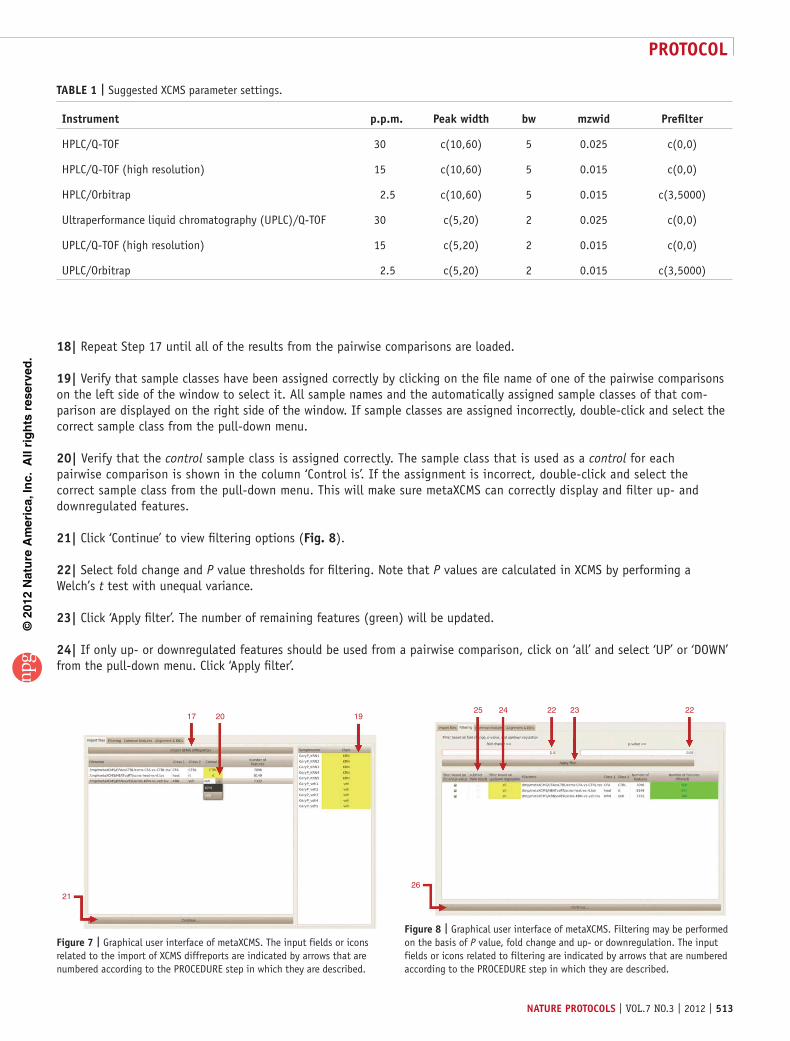
18| Repeat Step 17 until all of the results from the pairwise comparisons are loaded.

19| Verify that sample classes have been assigned correctly by clicking on the file name of one of the pairwise comparisons on the left side of the window to select it. All sample names and the automatically assigned sample classes of that com-parison are displayed on the right side of the window. If sample classes are assigned incorrectly, double-click and select the correct sample class from the pull-down menu.

20| Verify that the control sample class is assigned correctly. The sample class that is used as a control for each pairwise comparison is shown in the column ‘Control is’. If the assignment is incorrect, double-click and select the correct sample class from the pull-down menu. This will make sure metaXCMS can correctly display and filter up- and downregulated features.

21| Click ‘Continue’ to view filtering options (Fig. 8).

22| Select fold change and P value thresholds for filtering. Note that P values are calculated in XCMS by performing a Welch’s t test with unequal variance.

23| Click ‘Apply filter’. The number of remaining features (green) will be updated.

24| If only up- or downregulated features should be used from a pairwise comparison, click on ‘all’ and select ‘UP’ or ‘DOWN’ from the pull-down menu. Click ‘Apply filter’.

TABLE 1 | Suggested XCMS parameter settings.

Instrument p.p.m. Peak width bw mzwid Prefilter

HPLC/Q-TOF 30 c(10,60) 5 0.025 c(0,0)

HPLC/Q-TOF (high resolution) 15 c(10,60) 5 0.015 c(0,0)

HPLC/Orbitrap 2.5 c(10,60) 5 0.015 c(3,5000)

Ultraperformance liquid chromatography (UPLC)/Q-TOF 30 c(5,20) 2 0.025 c(0,0)

UPLC/Q-TOF (high resolution) 15 c(5,20) 2 0.015 c(0,0)

UPLC/Orbitrap 2.5 c(5,20) 2 0.015 c(3,5000)

17

21

20 19

Figure 7 | Graphical user interface of metaXCMS. The input fields or icons related to the import of XCMS diffreports are indicated by arrows that are numbered according to the PROCEDURE step in which they are described.

25

26

24 22 23 22

Figure 8 | Graphical user interface of metaXCMS. Filtering may be performed on the basis of P value, fold change and up- or downregulation. The input fields or icons related to filtering are indicated by arrows that are numbered according to the PROCEDURE step in which they are described.

©20

12 N

atur

e A

mer

ica,

Inc.

All

righ

ts r

eser

ved.

PROTOCOL

514 | VOL.7 NO.3 | 2012 | NATURE PROTOCOLS

25| If features from a pairwise comparison should be sub-tracted from the result (e.g., such as features altered in a sham control), select the ‘subtract from result’ checkbox.

26| Click ‘Continue’.

27| Adjust acceptable m/z and retention-time tolerance. Default values for HPLC/Q-TOF are 0.01 and 60 s.

28| Click ‘Find common features’. After the alignment has been calculated, a Venn diagram with the numbers of unique and common features between the pairwise comparisons will be shown (Fig. 9).

29| Save the Venn diagram as a .png or .pdf file.

30| To export a table with only the common features, click ‘Export common features table’.

31| To export a table with all features (unique, common and shared), click ‘Export all features table’.

32| Click ‘Continue’.

33| Click ‘Run Raw Data Alignment’. Retention-time correction for all samples will be recalculated (Fig. 10).? TROUBLESHOOTING

34| Click ‘Generate EICs for common features’. After an output folder for the EICs has been selected, EICs will be generated for all common features by using the data from all samples.? TROUBLESHOOTING

? TROUBLESHOOTINGTroubleshooting advice can be found in Table 2. If you see the error message: “Error: cannot allocate vector of size X Mb” (this might occur in any of Steps 10–13 and 17–34), it means that you have insufficient RAM. You will need to upgrade the RAM, and use a 64-bit operating system. If you experience problems not discussed here, please write a comment on this protocol and describe the problem in the XCMS/metaXCMS user forum at http://metlin.scripps.edu/xcms/faq.php.

27 28 27

31302932

KRN/veh

332

17

3

28

536CFA/CTRL 41

776heat/rt

Figure 9 | Graphical user interface of metaXCMS. Features that are uniquely or commonly altered among the pairwise comparisons are displayed as Venn diagrams. The icons related to data visualization and export are indicated by arrows that are numbered according to the PROCEDURE step in which they are described.

TABLE 2 | Troubleshooting table.

Step Problem Possible reason Solution

10 Error in xcmsSet(method = “centWave”): no NetCDF/mzXML/mzData/mzML files were found

Working directory does not contain any LC/MS raw data files

Make sure the correct folder is selected

16 Error in inDL(x, as.logical(local), as.logical(now), …): unable to load shared object ‘C:/Program Files/[…]/cairoDevice.dll’:

GTK + software is not installed

Install GTK + as described on http://metlin.scripps.edu/metaxcms/download.php

Error in inDL(x, as.logical(local), as.logical(now), …): unable to load shared object ‘C:/Program Files/[…]/RGtk2.dll’:

GTK+ software is not installed

Install GTK+ as described on http://metlin.scripps.edu/metaxcms/download.php

33 Cannot find the raw data files for X Raw data files have been deleted or moved

Do not rename or move the data folders and do not rename columns in the XCMS result table after XCMS processing

©20

12 N

atur

e A

mer

ica,

Inc.

All

righ

ts r

eser

ved.

PROTOCOL

NATURE PROTOCOLS | VOL.7 NO.3 | 2012 | 515

TIMINGThe total timing for the protocol is variable. Depending on the number of CPU cores used, XCMS processing (Steps 10–13) typically takes 15 min to 2 h per pairwise comparison. Depending on the number of samples and the file size, Steps 33 and 34 can take up to 1–2 h each.

ANTICIPATED RESULTSmetaXCMS will create tables with all features (unique, common and shared) in .csv format (comma separated values). The files can be opened by Microsoft Excel or Open Office and displayed as spreadsheets. Each row of the spreadsheet will corre-spond to a feature and list m/z values as well as retention-time values in addition to fold changes and P values (as originally calculated by XCMS) for each of the pairwise comparisons. EICs will be generated for each feature in the table and can be used for visual inspection. It is important to note that metaXCMS does not provide metabolite identifications. To identify interesting features, generally accurate masses are first searched in metabolite databases for making putative metabolite assignments. The putative assignments are subsequently confirmed by additional experiments comparing retention time and tandem MS data to those of model standards.

ACKNOWLEDGMENTS This work was supported by the California Institute of Regenerative Medicine (grant TR1-01219), the US National Institutes of Health (grants R24 EY017540-04, P30 MH062261-10 and P01 DA026146-02) and a US National Institutes of Health/National Institute on Aging grant (L30 AG0 038036; to G.J.P.). Financial support was also received from the US Department of Energy (grants FG02-07ER64325 and DE-AC0205CH11231).

AUTHOR CONTRIBUTIONS G.J.P., R.T. and G.S. contributed to the development of the protocol and the writing of the manuscript.

COMPETING FINANCIAL INTERESTS The authors declare no competing financial interests.

Published online at http://www.natureprotocols.com/. Reprints and permissions information is available online at http://www.nature.com/reprints/index.html.

1. Weckwerth, W. Unpredictability of metabolism—the key role of metabolomics science in combination with next-generation genome sequencing. Anal. Bioanal. Chem. 400, 1967–1978 (2011).

2. Baker, M. Metabolomics: from small molecules to big ideas. Nat. Meth. 8, 117–121 (2011).

3. Yanes, O. et al. Metabolic oxidation regulates embryonic stem cell differentiation. Nat. Chem. Biol. 6, 411–417 (2010).

4. Wikoff, W.R. et al. Metabolomics analysis reveals large effects of gut microflora on mammalian blood metabolites. Proc. Natl. Acad. Sci. USA 106, 3698–3703 (2009).

5. Wikoff, W.R., Pendyala, G., Siuzdak, G. & Fox, H.S. Metabolomic analysis of the cerebrospinal fluid reveals changes in phospholipase expression in the CNS of SIV-infected macaques. J. Clin. Invest. 118, 2661–2669 (2008).

6. Vinayavekhin, N. & Saghatelian, A. Untargeted metabolomics. Curr. Protoc. Mol. Biol. 90, 30.1.1–30.1.24 (2010).

7. Wikoff, W.R., Nagle, M.A., Kouznetsova, V.L., Tsigelny, I.F. & Nigam, S.K. Untargeted metabolomics identifies enterobiome metabolites and putative uremic toxins as substrates of organic anion transporter 1 (Oat1). J. Proteome Res. 10, 2842–2851 (2011).

8. Vinayavekhin, N., Homan, E.A. & Saghatelian, A. Exploring disease through metabolomics. ACS Chem. Biol. 5, 91–103 (2010).

9. McKnight, S.L. On getting there from here. Science 330, 1338–1339 (2010).

10. Wang, T.J. et al. Metabolite profiles and the risk of developing diabetes. Nat. Med. 17, 448–453 (2011).

11. Wang, Z. et al. Gut flora metabolism of phosphatidylcholine promotes cardiovascular disease. Nature 472, 57–63 (2011).

12. Dang, L. et al. Cancer-associated IDH1 mutations produce 2-hydroxyglutarate. Nature 462, 739–744 (2009).

13. Olszewski, K.L. et al. Branched tricarboxylic acid metabolism in Plasmodium falciparum. Nature 466, 774–778 (2010).

14. Fernie, A.R., Trethewey, R.N., Krotzky, A.J. & Willmitzer, L. Metabolite profiling: from diagnostics to systems biology. Nat. Rev. Mol. Cell Biol. 5, 763–769 (2004).

15. Lu, W. et al. Metabolomic analysis via reversed-phase ion-pairing liquid chromatography coupled to a stand-alone Orbitrap mass spectrometer. Anal. Chem. 82, 3212–3221 (2010).

16. Buscher, J.M., Czernik, D., Ewald, J.C., Sauer, U. & Zamboni, N. Cross-platform comparison of methods for quantitative metabolomics of primary metabolism. Anal. Chem. 81, 2135–2143 (2009).

17. Smith, C.A., Want, E.J., O Maille, G., Abagyan, R. & Siuzdak, G. XCMS: processing mass spectrometry data for metabolite profiling using nonlinear peak alignment, matching, and identification. Anal. Chem. 78, 779–787 (2006).

18. Yanes, O., Tautenhahn, R., Patti, G.J. & Siuzdak, G. Expanding coverage of the metabolome for global metabolite profiling. Anal. Chem. 83, 2152–2161 (2011).

19. Want, E.J. et al. Solvent-dependent metabolite distribution, clustering, and protein extraction for serum profiling with mass spectrometry. Anal. Chem. 78, 743–752 (2006).

100

50

0

0 1,000 2,000Retention time

Retention time deviation versus retention time GaryP_CFA1

Ret

entio

n tim

e de

viat

ion

3,000 4,000

GaryP_CFA2GaryP_CFA3GaryP_CFA4GaryP_CFA5GaryP_ctrl1GaryP_ctrl2GaryP_ctrl3GaryP_ctrl4GaryP_ctrl5GaryP_heat1GaryP_heat2GaryP_heat3GaryP_heat4GaryP_heat5GaryP_heat6GaryP_RT1GaryP_RT2GaryP_RT3GaryP_RT4GaryP_RT5GaryP_RT6GaryP_KRN1GaryP_KRN2GaryP_KRN3

33

34

Figure 10 | Graphical user interface of metaXCMS. Retention-time correction for all samples compared is displayed and EICs are generated. The icons related to retention-time correction and EIC generation are indicated by arrows that are numbered according to the PROCEDURE steps in which they are described.

©20

12 N

atur

e A

mer

ica,

Inc.

All

righ

ts r

eser

ved.

PROTOCOL

516 | VOL.7 NO.3 | 2012 | NATURE PROTOCOLS

20. Lommen, A. MetAlign: interface-driven, versatile metabolomics tool for hyphenated full-scan mass spectrometry data preprocessing. Anal. Chem. 81, 3079–3086 (2009).

21. Katajamaa, M., Miettinen, J. & Oresic, M. MZmine: toolbox for processing and visualization of mass spectrometry based molecular profile data. Bioinformatics 22, 634–636 (2006).

22. Böttcher, C. et al. The multifunctional enzyme CYP71B15 (PHYTOALEXIN DEFICIENT3) converts cysteine-indole-3-acetonitrile to camalexin in the indole-3-acetonitrile metabolic network of Arabidopsis thaliana. Plant Cell 21, 1830–1845 (2009).

23. Tautenhahn, R. et al. metaXCMS: second-order analysis of untargeted metabolomics data. Anal. Chem. 83, 696–700 (2011).

24. Normand, S.L. Meta-analysis: formulating, evaluating, combining, and reporting. Stat. Med. 18, 321–359 (1999).

25. Willer, C.J., Li, Y. & Abecasis, G.R. METAL: fast and efficient meta-analysis of genomewide association scans. Bioinformatics 26, 2190–2191 (2010).

26. de Bakker, P.I. et al. Practical aspects of imputation-driven meta-analysis of genome-wide association studies. Hum. Mol. Genet. 17, R122–R128 (2008).

27. de Bakker, P.I. et al. Efficiency and power in genetic association studies. Nat. Genet. 37, 1217–1223 (2005).

28. Chu, Y.C. et al. Effect of genetic knockout or pharmacologic inhibition of neuronal nitric oxide synthase on complete Freund s adjuvant-induced persistent pain. Pain 119, 113–123 (2005).

29. Bolcskei, K., Petho, G. & Szolcsanyi, J. Noxious heat threshold measured with slowly increasing temperatures: novel rat thermal hyperalgesia models. Methods Mol. Biol. 617, 57–66 (2010).

30. Kyburz, D. & Corr, M. The KRN mouse model of inflammatory arthritis. Springer Semin. Immunopathol. 25, 79–90 (2003).

31. Goo, Y.A. et al. Proteomic analysis of an extreme halophilic archaeon, Halobacterium sp. NRC-1. Mol. Cell Proteomics 2, 506–524 (2003).

32. Kaur, A. et al. A systems view of haloarchaeal strategies to withstand stress from transition metals. Genome Res. 16, 841–854 (2006).

33. Branca, F., Hanley, A.B., Pool-Zobel, B. & Verhagen, H. Biomarkers in disease and health. Br. J. Nutr. 86 (suppl. 1): S55–S92 (2001).

34. Cantor, R.M., Lange, K. & Sinsheimer, J.S. Prioritizing GWAS results: a review of statistical methods and recommendations for their application. Am. J. Hum. Genet. 86, 6–22 (2010).

35. Crews, B. et al. Variability analysis of human plasma and cerebral spinal fluid reveals statistical significance of changes in mass spectrometry–based metabolomics data. Anal. Chem. 81, 8538–8544 (2009).

36. Kalisiak, J. et al. Identification of a new endogenous metabolite and the characterization of its protein interactions through an immobilization approach. J. Am. Chem. Soc. 131, 378–386 (2009).

37. Wise, L.H., Lanchbury, J.S. & Lewis, C.M. Meta-analysis of genome searches. Ann. Hum. Genet. 63, 263–272 (1999).

38. Evangelou, E., Maraganore, D.M. & Ioannidis, J.P. Meta-analysis in genome-wide association datasets: strategies and application in Parkinson disease. PLoS ONE 2, e196 (2007).

39. Want, E.J., Nordstrom, A., Morita, H. & Siuzdak, G. From exogenous to endogenous: the inevitable imprint of mass spectrometry in metabolomics. J. Proteome Res. 6, 459–468 (2007).

40. Tautenhahn, R., Böttcher, C. & Neumann, S. Highly sensitive feature detection for high-resolution LC/MS. BMC Bioinformatics 9, 504 (2008).

41. Prince, J.T. & Marcotte, E.M. Chromatographic alignment of ESI-LC-MS proteomics data sets by ordered bijective interpolated warping. Anal. Chem. 78, 6140–6152 (2006).

42. Masson, P., Spagou, K., Nicholson, J.K. & Want, E.J. Technical and biological variation in UPLC-MS–based untargeted metabolic profiling of liver extracts: application in an experimental toxicity study on galactosamine. Anal. Chem. 83, 1116–1123 (2011).