mesoscale modeling of central american smoke transport to

Mesoscale modeling of Central American smoke transport to the

United States:

2. Smoke radiative impact on regional surface energy budget and

boundary layer evolution

Jun Wang1,2 and Sundar A. Christopher1

Received 28 September 2005; revised 16 December 2005; accepted 3 March 2006; published 26 July 2006.

[1] During 20 April to 21 May 2003, large amounts of smoke aerosols from CentralAmerican Biomass Burning (CABB) fires were transported to southeastern United States.Using a coupled aerosol, radiation, and meteorology model built upon the heritage of theRegional Atmospheric Modeling System (RAMS) with new capabilities called theAssimilation and Radiation Online Modeling of Aerosols (AROMA), this paper, thesecond of a two-part series, investigates smoke radiative impact on the regional surfaceenergy budget, temperature and relevant boundary layer processes. Comparisons withlimited ground-based observations and MODIS aerosol optical thickness (AOT) showedthat model consistently simulated the smoke AOT and smoke radiative impacts on the 2 mair temperature (2mT) and downward shortwave irradiance (DSWI). Over 30 days the24-hour mean smoke AOT was 0.18 (at 0.55 mm) near the smoke source region (YucatanPeninsula and southern Mexico), and 0.09 in downwind region (e.g., southern Texas),both showing a diurnal variation of 24%. Maximum AOT occurred during late afternoonand minimum during early morning in smoke source region. The smoke radiative effectswere dominant mostly during the daytime and resulted in the decrease of DSWI, sensibleheat and latent heat by 22.5 Wm�2, 6.2 Wm�2, and 6.2 Wm�2, respectively, near thesource region, in contrast to 15.8 Wm�2, 4.7 Wm�2, and 7.9 Wm�2, respectively, indownwind regions. Both maximum and minimum 2mT were decreased, and the overalldiurnal temperature range (DTR) was reduced by 0.31�C and 0.26�C in the smoke sourceand downwind regions, respectively. The smoke absorption of solar radiation increased thelapse rate by 0.1–0.5 K/day in the planetary boundary layer (PBL), thus warming theair over the ocean surface. However, over the land surface where the coupling betweenthe lower PBL and the cooler land surface is strong, such warming only occurred in theupper PBL and is amendable to the diurnal variation of smoke emission. The simulationnumerically verifies the smoke self-trapping feedback mechanism proposed by Robock(1988), where the increase of the atmospheric stability in the PBL caused by the smokeradiative effects further traps more smoke aerosols in the lower PBL. Such feedbacks,when coupled with favorable synoptic systems, may have important implications for airquality modeling and hydrological processes.

Citation: Wang, J., and S. A. Christopher (2006), Mesoscale modeling of Central American smoke transport to the United States:

2. Smoke radiative impact on regional surface energy budget and boundary layer evolution, J. Geophys. Res., 111, D14S92,

doi:10.1029/2005JD006720.

1. Introduction

[2] Widely occurring in the tropics, biomass burningis one of the largest sources of anthropogenic aerosols

[Crutzen and Andreae, 1990]. Burning mostly occurs dur-ing the tropical dry season (e.g., April–June in the northernhemisphere and August–October in the southern hemi-sphere), and ends when wet season begins [Crutzen et al.,1979]. Smoke particles from burning fires degrade thevisibility and air quality in both source and downwindregions [Peppler et al., 2000], and have important implica-tions for climate and weather forecasting, since they affectthe atmospheric radiative transfer both directly (by scatter-ing the sunlight) and indirectly (by acting as cloud conden-sation nuclei) [Twomey, 1977; Penner et al., 1992]. Inaddition, the black carbon in smoke particles strongly

JOURNAL OF GEOPHYSICAL RESEARCH, VOL. 111, D14S92, doi:10.1029/2005JD006720, 2006ClickHere

for

FullArticle

1Department of Atmospheric Science, University of Alabama, Hunts-ville, Alabama, USA.

2Now at Division of Engineering and Applied Science and Departmentof Earth and Planetary Science, Harvard University, Cambridge, Massa-chusetts, USA.

Copyright 2006 by the American Geophysical Union.0148-0227/06/2005JD006720$09.00

D14S92 1 of 17

http://dx.doi.org/10.1029/2005JD006720

absorb solar radiation [Jacobson, 2001], thereby enhancingthe atmospheric radiative heating rate, modifying the atmo-spheric stability [Robock, 1988] and altering cloud forma-tion [Ackerman et al., 2000; Koren et al., 2004], which canpossibly result in measurable changes in precipitation dis-tribution [Menon et al., 2002]. Accurate representation ofsmoke radiative impacts is crucial for the prediction ofclimate and weather [Ramanathan et al., 2001; Intergov-ernmental Panel on Climate Change (IPCC), 2001], par-ticularly during the biomass-burning season in regionalscales [Westphal and Toon, 1991; Kaufman et al., 1998;Swap et al., 2003].[3] During April–May 2003, under the influence of

southerly flow, large amounts of smoke aerosols from theCentral American Biomass Burning (CABB) were trans-ported across the Gulf of Mexico and reached the Texas,Oklahoma, and other nearby areas in the southeasternUnited States (SEUS) [Wang et al., 2006]. The events arethe second largest in the last decade in this region (after theMay 1998 CABB events [Peppler et al., 2000]), andresulted in the largest PM2.5 (particulate matter with aero-dynamic diameter less than 2.5 mm) mass concentrationmeasured in southern Texas since 1998 [Wang et al., 2006].The intent of this study is to investigate the direct radiativeimpacts of smoke events on the surface energy budget, airtemperature, and evolution of planetary boundary layer(PBL) in both the source and downwind regions.[4] A wealth of previous studies using combinations of

measurements and chemistry transport models (CTM), havebeen carried out to examine smoke radiative impacts,particularly in quantifying the direct smoke radiative forcingat the top of atmosphere (TOA) (see IPCC [2001, section6.7.5] for a review). These studies reported that the TOAglobal direct radiative forcing of biomass-burning smokeaerosols is �0.2 Wm�2 with an uncertainty of at least of300%. However, the magnitude could be one to two orderslarger in the smoke source region during biomass-burningseasons. While smoke radiative forcing at TOA is impor-tant, equally important is the forcing at the surface as well asin the atmosphere. Both model calculations and measure-ments have showed that the smoke radiative forcing at thesurface is about 2�3 times larger than the forcing at TOAdue to the enhancement by smoke absorption in the atmo-sphere [Christopher et al., 2000; Schafer et al., 2002]. Theimportance of such forcing on the surface energy budgetand PBL evolution has been noted by numerous earlierstudies [e.g., Atwater et al., 1971a, 1971b; Bergstrom, 1973;Ackerman, 1977; Carlson and Benjamin, 1980]. Recently,Yu et al. [2002] showed that, for a smoke layer with aerosoloptical thickness (AOT) of 0.5 and single scattering albedolarger than 0.9 in the PBL, absorption of solar radiation canincrease the daytime radiative heating in the PBL up to52 Wm�2, and its extinction on the downward shortwaveirradiance (DSWI) can result in the decrease of surface skintemperature more than 1 K. They further showed that thesechanges, when coupled with the PBL processes, can causemeasurable decrease of PBL height (PBLH) and diurnaltemperature range (DTR). While these studies advanced ourunderstanding on the aerosol radiative impacts in the lowertroposphere, they were carried out in a ‘‘1D’’ columnframework (e.g., no horizontal advection). In contrast,CTMs reasonably simulate the 3D aerosol distribution at

regional and global scales [Liousse et al., 1996; Tegen et al.,1997; Chin et al., 2002; Park et al., 2003; Carmichael et al.,2003; Colarco et al., 2004], but most of them are driven bymeteorological fields (such as winds) from offline meteo-rological models. As such, coupling the aerosol transportand aerosol radiation with a 3D meteorological modelwould be important for further investigation on the meteo-rological responses to the smoke radiative effects [Westphaland Toon, 1991; Wang et al., 2004].[5] In traditional meteorological models, aerosol radiative

impacts are not explicitly treated, because aerosol distribu-tion with high spatiotemporal variations is not readilyavailable in the model [Stephens, 1984]. This could causelarge uncertainties in the simulation of surface energybudget, particularly during the smoke or dust episodes[Ackerman and Cox, 1982; Stephens, 1984; Cautenet etal., 1992; Chen et al., 1995]. Robock [1988] reported thatsmoke emitted from forest fires in northern California inSeptember 1987 was trapped in a valley by an inversionlayer for nearly 3 weeks. This smoke layer decreased thedaily maximum air temperature near the surface by morethan 15�C below normal conditions for about 1 week andmore than 5�C for 3 weeks. He proposed that the mainte-nance of this long-term inversion layer was due a positivefeedback loop where the smoke layer blocks the solarradiation from reaching the surface while absorbing thesolar energy in the atmosphere, thus triggering a favorablemechanism for the temperature inversion that in turnenhances the smoke trapping. Westphal and Toon [1991]showed a case study where the surface temperature wasdecreased by 5�C during the passage of smoke plumes froma boreal fire in 1988. In the Nashville southern oxidantsstudies in 1995 and 1999, Zamora et al. [2003] found thatthe incorrect (neglecting) specification of aerosol scatteringand absorption in the Fifth-Generation Penn State/NCARMesoscale Model (MM5) can lead to an overestimation ofDSWI by 100 Wm�2, and suggested that aerosol radiativeprocess is important for both meteorological and air qualityforecasting. Recently, Grell et al. [2004] has proposed toincorporate the aerosol-radiation interaction in the WeatherResearch and Forecast (WRF) model, and Wang et al.[2004] have reported improvement in the simulation ofsurface energy budget and air temperature during the dusttransport after incorporating the dust radiative impacts in theRegional Atmospheric Modeling System (RAMS).[6] Since aerosol radiative effects are absent in most

standard mesoscale meteorological models such as MM5[Grell et al., 1995] or RAMS [Harrington and Olsson,2001; Cotton et al., 2003], previous studies have employedclimate models (such as Community Climate Model CCM3)to investigate the smoke radiative impacts [Chung andZhang, 2004; Davison et al., 2004]. However, these inves-tigations usually lack detailed treatment of smoke temporalvariations, i.e., smoke distribution and vertical profile wereeither specified as time-invariant [Chung and Zhang, 2004]or were simulated by adopting the constant smoke emissionrate [Davison et al.,2004]. Such simplification may lead toconsiderable uncertainties in the model results, becauseaerosol radiative impact highly depends on the solar zenithangle [Christopher and Zhang, 2002] as well as the aerosolvertical distribution [Yu et al., 2002; Feingold et al., 2005],both amenable to the distinct diurnal behavior of biomass-

D14S92 WANG AND CHRISTOPHER: 3D MODELING OF SMOKE RADIATIVE IMPACT

2 of 17

D14S92

burning activities with peak in the noon time and minimumduring the night [Prins et al., 1998]. Using data collected insouthern Africa during the Southern African RegionalScience Initiative (SAFARI) campaign, Eck et al. [2003]reported that such fire behavior can lead to a 25% systemicdiurnal variation of smoke AOT with maximum (minimum)at local 1800 LT (1000 LT) near the smoke source regioneven over a monthly scale.[7] In this study, we investigate the CABB smoke

radiative impacts and feedbacks using a coupled aerosol-radiation-meteorology model, a modified version of RAMSwith newly developed capabilities of Assimilation andRadiation Online Modeling of Aerosols (RAMS-AROMA)[Wang et al., 2004, 2006]. RAMS-AROMA couples theaerosol radiation and aerosol transport together with mete-orology [Wang et al., 2004], and realistically specifies thediurnal variation of the smoke emission rate by assimilatingthe hourly geostationary satellite-derived smoke emissionproduct into the model [Wang et al., 2006]. In the first of thistwo-part series study [Wang et al., 2006], we have usedRAMS-AROMA to simulate the CABB smoke transportduring 20 April to 21 May 2003, and showed that thesimulation was able to capture diurnal variation of AOT inthe smoke source region. Comparison with a variety ofground measurements such as PM2.5 concentration, carbonmass concentration and AOT, demonstrated the success ofRAMS-AROMA in simulating the spatiotemporal variationsof smoke distribution [Wang et al., 2006].[8] Since a comprehensive validation of RAMS-AROMA

performance in modeling the smoke distribution has beenconducted byWang et al. [2006], in this paper we will studythe smoke radiative impacts mainly on the basis of theanalysis of model results. Similar to previous studies[Westphal and Toon, 1991; Menon et al., 2002; Davison etal., 2004; Chung and Zhang, 2004], this study uses RAMS-AROMA to examine the large-scale aerosol radiative impactson surface energy budget and feedbacks on atmosphericprocesses that otherwise would be difficult to investigatefrom observations alone. A brief description of the model,experiment design and data used for the validation is given insection 2. Results are presented in section 3 and the discussionand conclusion are given in section 4.

2. Model Description, Experiment Design, andData Used

2.1. Model Description

[9] The RAMS-AROMA is developed upon the RAMS4.3 [Pielke et al., 1992], and a detailed description is givenby Wang et al. [2004, 2006] and Wang [2005]. In RAMS-AROMA, a d-4 Stream (4S) Radiative Transfer Model(RTM) [Fu and Liou, 1993] is embedded in place of theoriginal two-stream RTM to take into account the impact ofboth cloud and aerosol on the radiative transfer. While theRAMS4.3 has a tracer advection module that can be used tosimulate the aerosol transport, it does not include anyaerosol deposition or source functions. In RAMS-AROMA,we have added several components for modeling aerosolwet and dry deposition processes. More importantly wehave developed the assimilation routine of using GOES-derived hourly smoke emission data [Reid et al., 2004;Prins et al., 1998] for specifying the smoke source function

[Wang et al., 2006]. In summary, RAMS-AROMA not onlymaintains all the functionalities of RAMS4.3 (e.g., meteo-rological forecast), but also has new capabilities to simulatethe aerosol fields and accounts for the aerosol radiativeimpacts explicitly at each time step and in each model grid.With this design, the aerosol radiative impacts are directlytied to the simulated physical processes in the atmosphere,allowing the dynamical processes in the model to impactaerosol transport and vice versa.[10] In calculating the smoke radiative impacts, wave-

length-dependent smoke optical properties (such as singlescattering albedo, extinction cross section and asymmetricfactor) are needed to convert the smoke mass concentrationinto the smoke AOT, and are further used in the d-4S RTMto compute smoke radiative effects. In RAMS-AROMA, thesmoke AOT is calculated by

t ¼XK

i¼1

Qm � Ci � f rhið Þð Þ � Dzi;

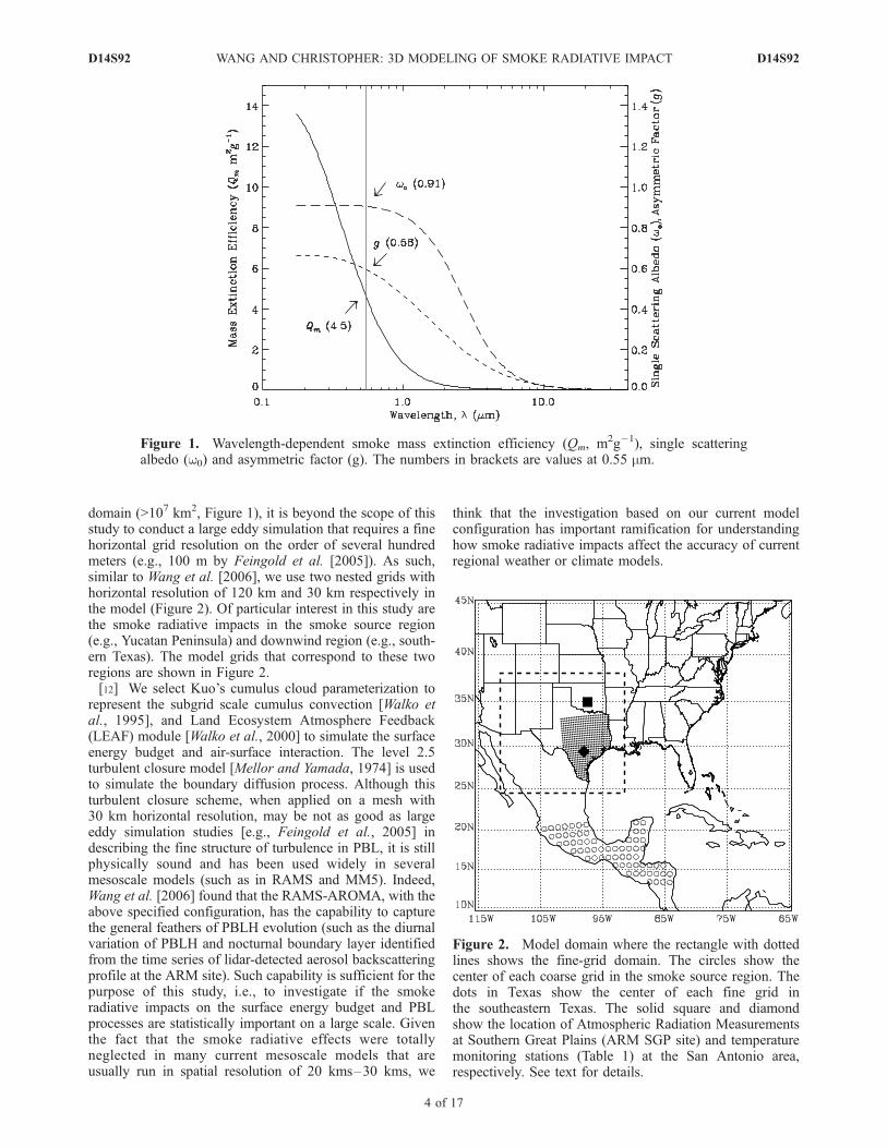
where i is the index for vertical layers, K is the total numberof layers in the model, C is the mass concentration of smoke(gm�3), Qm is the mass extinction efficiency (m2g�1) ofsmoke particles, Dzi is the thickness (m) of different layers,and f(rh) is the hygroscopic factor as a function of relativehumidity (rh) [Kotchenruther and Hobbs, 1998]. In thisstudy, we used the smoke optical model developed byChristopher and Zhang [2002] where Qm is calculated onthe basis of Mie theory by modeling smoke particles as ablack carbon core surrounded by an organic shell. Theorganic shell is assumed as nonabsorbing with real partindex of refraction of 1.5 [Reid et al., 2005]. The refractiveindex of black carbon is adapted from Chang andCharalampopoulos [1990]. The density of black carbonand organic carbon is assumed to be 1.8gcm�3 and1.2gcm�3, respectively. The radius ratio of the core andshell is assumed to be 0.3 with an equivalent mass fractionof black carbon of 4%. To obtain the bulk optical properties,smoke size distribution is assumed to be lognormal withvolume mean diameter of 0.3 mm and standard deviation of1.8 mm. With these parameters, the modeled singlescattering albedo at 0.55 mm and 0.67 mm are 0.91 and0.90 respectively, consistent with values that are mostlyused in the current literature (see review paper by Reid et al.[2005]). Figure 1 shows the calculated single scatteringalbedo, asymmetric factor, and mass extinction coefficientat different wavelengths. At 0.55 mm, the mass extinctionefficiency is about 4.5 m2g�1.

2.2. Experiment Design and Data Used

[11] The model configuration is the same as Wang et al.[2006] where the simulation started at 1200 UTC on20 April 2003, and ended at 1200 UTC on 21 May 2003.The vertical intervals are 50 m at the lowest layer andgradually expand upward to the maximum value of 700 mwith a stretch ratio of 1.2. With this configuration, ourmodel vertical resolution in the PBL is only slightly coarserthan those used in previous large-eddy simulations that arebelieved to be an ideal tool for simulating the PBL processin detail (e.g., Feingold et al. [2005] used 50 m interval forall vertical layers). However, because of our large study


3 of 17

D14S92

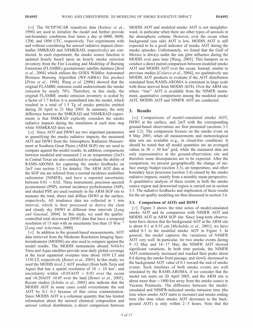
domain (>107 km2, Figure 1), it is beyond the scope of thisstudy to conduct a large eddy simulation that requires a finehorizontal grid resolution on the order of several hundredmeters (e.g., 100 m by Feingold et al. [2005]). As such,similar to Wang et al. [2006], we use two nested grids withhorizontal resolution of 120 km and 30 km respectively inthe model (Figure 2). Of particular interest in this study arethe smoke radiative impacts in the smoke source region(e.g., Yucatan Peninsula) and downwind region (e.g., south-ern Texas). The model grids that correspond to these tworegions are shown in Figure 2.[12] We select Kuo’s cumulus cloud parameterization to

represent the subgrid scale cumulus convection [Walko etal., 1995], and Land Ecosystem Atmosphere Feedback(LEAF) module [Walko et al., 2000] to simulate the surfaceenergy budget and air-surface interaction. The level 2.5turbulent closure model [Mellor and Yamada, 1974] is usedto simulate the boundary diffusion process. Although thisturbulent closure scheme, when applied on a mesh with30 km horizontal resolution, may be not as good as largeeddy simulation studies [e.g., Feingold et al., 2005] indescribing the fine structure of turbulence in PBL, it is stillphysically sound and has been used widely in severalmesoscale models (such as in RAMS and MM5). Indeed,Wang et al. [2006] found that the RAMS-AROMA, with theabove specified configuration, has the capability to capturethe general feathers of PBLH evolution (such as the diurnalvariation of PBLH and nocturnal boundary layer identifiedfrom the time series of lidar-detected aerosol backscatteringprofile at the ARM site). Such capability is sufficient for thepurpose of this study, i.e., to investigate if the smokeradiative impacts on the surface energy budget and PBLprocesses are statistically important on a large scale. Giventhe fact that the smoke radiative effects were totallyneglected in many current mesoscale models that areusually run in spatial resolution of 20 kms–30 kms, we

think that the investigation based on our current modelconfiguration has important ramification for understandinghow smoke radiative impacts affect the accuracy of currentregional weather or climate models.

Figure 1. Wavelength-dependent smoke mass extinction efficiency (Qm, m2g�1), single scatteringalbedo (w0) and asymmetric factor (g). The numbers in brackets are values at 0.55 mm.

Figure 2. Model domain where the rectangle with dottedlines shows the fine-grid domain. The circles show thecenter of each coarse grid in the smoke source region. Thedots in Texas show the center of each fine grid inthe southeastern Texas. The solid square and diamondshow the location of Atmospheric Radiation Measurementsat Southern Great Plains (ARM SGP site) and temperaturemonitoring stations (Table 1) at the San Antonio area,respectively. See text for details.


4 of 17

D14S92

[13] The NCEP/NCAR reanalysis data [Kalnay et al.,1996] are used to initialize the model and further provideout-boundary conditions four times a day at 0000, 0600,1200, and 1800 UTC, respectively. Two experiments withand without considering the aerosol radiative impacts (here-inafter SMKRAD and NSMKRAD, respectively) are con-ducted. In each experiment, the smoke source function isupdated hourly based upon an hourly smoke emissioninventory from the Fire Locating and Modeling of BurningEmissions (FLAMBE) geostationary satellite database [Reidet al., 2004] which utilizes the GOES Wildfire AutomatedBiomass Burning Algorithm (WF-ABBA) fire product[Prins et al., 1998]. Wang et al. [2006] showed that theoriginal FLAMBE emission could underestimate the smokeemission by nearly 70%. Therefore, in this study, theoriginal FLAMBE smoke emission inventory is scaled bya factor of 1.7 before it is assimilated into the model, whichresulted in a total of 1.5 Tg of smoke particles emittedduring 20 April to 21 May 2003. In summary, the onlydifference between the SMKRAD and NSMKRAD experi-ments is that SMKRAD explicitly considers the smokeradiative impacts during the simulation at each time stepwhile NSMKRAD does not.[14] Since AOT and DSWI are two important parameters

in quantifying the smoke radiative impacts, the measuredAOT and DSWI from the Atmospheric Radiation Measure-ment at Southern Great Plains (ARM SGP) site are used tocompare against the model results. In addition, comparisonsbetween modeled and measured 2 m air temperature (2mT)in Central Texas are also conducted to evaluate the ability ofRAMS-AROMA for capturing the smoke feedbacks on2mT (see section 3.2 for details). The ARM AOT data atthe SGP site are inferred from a normal incidence multifilterradiometer (NIMFR), and have a reported uncertaintybetween 0.01 � 0.02. Three instruments, precision spectralpyranometer (PSP), normal incidence pyrheliometer (NIP),and shaded PSP, are used routinely in the ARM SGP site tomeasure the total, direct and diffuse DSWI at the surface,respectively. All irradiance data are collected in 1 mininterval, which is then processed to derive the clearand cloudy sky DSWI in different time intervals [Longand Gaustad, 2004]. In this study, we used the quality-controlled total downward DSWI data that have a temporalresolution of 15 min with an uncertainty less than 15 Wm�2

[Long and Ackerman, 2000].[15] In addition to the ground-based measurements, AOT

data retrieved from the Moderate Resolution Imaging Spec-troradiometer (MODIS) are also used to compare against themodel results. The MODIS instruments aboard NASA’sTerra and Aqua satellites provide near daily global coverageat the local equatorial overpass time about 1030 LT and1330 LT, respectively [Remer et al., 2005]. In this study, weused the MODIS level 2 AOT product (from both Terra andAqua) that has a spatial resolution of 10 � 10 km2, anduncertainty within ±0.05AOT ± 0.03 over the oceanand ±0.20AOT ±0.05 over the land [Remer et al., 2005].Recent studies [Ichoku et al., 2005] also indicate that theMODIS AOT in some cases could overestimate the realAOT by 0.1–0.3 because of thin cirrus contamination.Since MODIS AOT is a columnar quantity that has limitedinformation about the aerosol chemical composition andaerosol vertical distribution, a direct comparison between

MODIS AOT and modeled smoke AOT is not straightfor-ward, in particular when there are other types of aerosols inthe atmospheric column. However, over the ocean whenbackground (sea salt) AOT is low, MODIS AOT is stillexpected to be a good indicator of smoke AOT during thesmoke episodes. Unfortunately, we found that the Gulf ofMexico is always under the sun glint influence during theMODIS over pass time [Wang, 2005]. This hampers us toconduct a direct paired comparison between modeled smokeAOT and MODIS AOT over the ocean. Instead, similar toprevious studies [Colarco et al., 2004], we qualitatively useMODIS AOT products to evaluate if the AOT distributionsimulated from RAMS-AROMA is consistent in large scalewith those derived from MODIS AOTs. Over the ARM sitewhere ‘‘true’’ AOT is available from the NIMFR instru-ment, quantitative comparisons among the modeled smokeAOT, MODIS AOT and NIMFR AOT are conducted.

3. Results

[16] Comparisons of model-simulated smoke AOT,DSWI at the surface, and 2mT with the correspondingground-based observations are first presented (sections 3.1and 3.2). The comparison focuses on the smoke event on8 May 2003, when all measurements and meteorologicaldata sets are available (e.g., in cloud-free condition). Itshould be noted that all model quantities are an averagedvalues in 30 � 30 km2 grid, while the measured data areonly representative at the ground-observation site andtherefore some discrepancies are to be expected. After thecomparison, we present geographically the change of sur-face energy budget (section 3.3), air temperature, and otherboundary layer processes (section 3.4) caused by the smokeradiative impacts, mainly from a monthly mean perspective.A quantitative analysis of these results in both the smokesource region and downwind region is carried out in section3.5. The radiative feedbacks and implication of these resultsfor the air quality modeling are then discussed in section 3.6.

3.1. Comparison of AOTs and DSWI

[17] Figure 3 shows the time series of model-simulatedsmoke AOT and its comparison with NIMFR AOT andMODIS AOT at ARM SGP site. Since long-term observa-tions have shown that the background AOT at the ARM siteis about 0.1 at 0.55 mm [Michalsky et al., 2001], we haveadded 0.1 to the modeled smoke AOT in Figure 3. Ingeneral, the model captures the variations of NIMFRAOT very well. In particular, for two smoke events during9–12 May and 14–17 May, the NIMFR AOT showedsignificant variations. In both time periods, the NIMFRAOT continuously increased and reached their peaks about0.4 during the smoke front passage, and slowly decreased tothe background AOT value of 0.1 toward the end of smokeevents. Such timelines of both smoke events are wellsimulated by the RAMS-AROMA, if we consider that themodel run starts on 20 April 2005, and the ARM site isabout more than �1800 km away from the smoke source inYucatan Peninsula. The difference between the model-simulated and NIMFR-indicated smoke intrusion time (thetime when smoke AOT starts to increase) and smoke endingtime (the time when smoke AOT decreases to the back-ground AOT) is only within 2–5 hours. Note that the


5 of 17

D14S92

Angstrom exponents decreased during the smoke events(Figure 3), which is consistent with the results of Andrews etal. [2004] who used 2 years of ARM data sets and showedthat long-range transported smoke aerosols usually result inthe decrease of the Angstrom exponent at the ARM site.Quantitatively, the modeled smoke AOT is smaller thanNIMFR AOT, even after the background AOT is taken intoaccount since there are other aerosols such as sulfate thatwere being transported to the ARM site along with thesmoke plumes [Wang et al., 2006]. In addition, becauseNIMFR AOTs only represent the AOTs at the observationpoint, the difference between the modeled and measuredAOT could also be due to the inability of the currentRAMS-AROMA to resolve the nonhomogeneity smokedistribution in the 30 � 30 km2 grid.[18] Similarly, a reasonable agreement can be found

between the modeled smoke AOT and the MODIS AOT,except on 14 May where the MODIS AOT seems to bemuch higher than modeled smoke AOT. The large spatialvariations (standard deviation bar) of MODIS AOT aroundthe AMR SGP site indicate a possible cloud contaminationin the MODIS AOT retrieval on that day. More interestingly,on 14 May when there are no valid MODIS AOT retrievals,implying at least partially cloudy conditions over the ARMsite. The NIFMR on the other hand showed high AOTs,implying clear sky conditions at the NIFMR site. Thisdemonstrates that the air mass is very inhomogeneous on14 May; another possible reason for the large differencebetween modeled and NIFMR AOT. Nevertheless, althoughonly a few MODIS AOT points (7 out of 20 days) areavailable at the ARM SGP site during the study period, their

reasonable agreement with modeled smoke AOT is encour-aging because MODIS AOT are grid (not point) quantities.The general consistency of modeled smoke AOT with theMODIS AOT and NIMFR AOT provides the basis forcomputing the smoke radiative impacts realistically inRAMS-AROMA.[19] Figure 4 shows the comparison of DSWI at surface at

the ARM SGP site on 8 May, 2003. The daytime averagesof the modeled smoke AOT on this day is the largest duringthe study time period, thus facilitating us to illustrate thesmoke radiative impacts on DSWI. The diurnal variation ofDSWI is well simulated in both SMKRAD and NSMKRADcases (Figure 4a). Because the radiative extinction ofatmospheric smoke layers attenuates the solar radiation,less DSWI is expected to reach the surface during thesmoke events such as on 8 May. This is the reason thatthe DSWI in NSMDRAD case is consistently larger than themeasured DSWI and SMKRAD-simulated DSWI. TheSMKRAD also overestimates the measured DSWI, possiblybecause the scattering of background aerosols (of AOTabout 0.1 and other type of aerosols associated with smokeplumes) has not been incorporated in the radiative transfercalculations. Depending on the solar zenith angle andsmoke AOT values, the simulated DSWI in NSWKRADcase overestimate the measured DSWI by 25–65 Wm�2,larger than the overestimation of 0–40 Wm�2 in SMKRADcase (Figure 4b). Overall, SMKRAD gives a better agree-ment with the measured DSWI, particularly during highsmoke AOT conditions (e.g., morning to early afternoon on8 May). The difference in DSWI between NSMKRAD andSMKRAD cases is about 20 Wm�2 on 8 May. This

Figure 3. Time series (in CDT, Central Daylight Time) of NIFMR-measured AOT (blue dots), MODISAOT from Terra (red dots) and Aqua (red squares) and modeled smoke AOT (pink line) at the ARM SGPsite. Bars in blue and green show the daily averaged AOT and Angstrom exponents derived from theNIMFR AOT, respectively. The MODIS AOT values and their error bars are reported, respectively, as themean and ±1 standard deviation of 3X3 MODIS AOT retrievals centered at the ARM SGP site. Note thatto compensate the lack of background AOT in the model, all modeled smoke AOT have been added 0.1(dashed line).


6 of 17

D14S92

difference is expected to be much larger in the smoke sourceregion, since the smoke AOT is usually (2–5 times) smallerat the ARM SGP site than in the source region or even thesouthern Texas. Unfortunately, the lack of ground-basedirradiance measurements along the smoke path way (fromthe Yucatan Peninsula to southern Texas) hampers us toconduct more comparisons.

3.2. Comparison of 2mT

[20] The accurate prediction of surface air temperaturedepends on many factors including the realistic representa-tion of dynamical and thermodynamic processes, the accu-rate description of land surface processes, and the reliableparameterization of turbulent processes in PBL. A betterestimation of surface energy input can therefore improve themodeling of surface energy budget and in turn the airtemperature near the surface. This postulation is evaluatedby comparing the RAMS-AROMA simulated 2 m airtemperature (2mT) with the measured 2mT in San Antonio,Texas. We selected the San Antonio region as the focusregion for several reasons. First, it is located in the southernpart of Central Texas (Figure 2) where the mass concentra-tion of transported smoke particles is larger than those innorthern Texas [Wang et al., 2006]. This makes the impact

of smoke layers on the 2mT in this region more distin-guishable. Secondly, in the San Antonio region, there are4 meteorological stations (see Table 1) from which theaveraged 2mT in this region can be better inferred thanfrom a single station alone. This advantage facilitates thecomparison with the modeled 2mT values that are averagedquantities over each 30�30 km2 grid. Thirdly, the SanAntonio region is far away from the coast of Gulf ofMexico and sea breeze has negligible impact on 2mT inthis region. In summary, we conduct the comparison be-tween model and observation in an optimal situation so thatthe smoke radiative impacts on 2mT can be favorablyidentified.[21] Figure 5 shows the comparison between modeled

and measured 2mT in San Antonio, Texas, on 8 May 2003.On this day, the modeled smoke AOT in San Antonio isabout 0.35 (figure not shown). Two model grids cover theSan Antonio region, and there are two meteorologicalstations collocated within each grid. In either grid(Figures 5a and 5b), the simulations from SMKRAD andNSMRAD cases demonstrate a consistent diurnal tempera-ture pattern with those from observations. Quantitatively,the modeled 2mT in SMKRAD case is about 0.3�C smallerthan that in NSMKRAD case, because smoke radiative

Figure 4. (a) Diurnal variation of modeled and measured downward shortwave irradiance (DSWI) atthe surface at the ARM SGP site on 8 May 2003. The modeled DSWI are reported from two modelexperiments with (solid line) and without (dotted line) considering smoke radiative effects (e.g.,SMKRAD and NSMKRAD), respectively. (b) Difference between measured and modeled DSWI(DDSWI) at the surface in SMKRAD (solid circles) and NSMKRAD (open circles), respectively. Alsoshown are the modeled smoke AOT (dotted line) and the difference of DSWI between SMKRAD andNSMKRAD cases (e.g., NSMKRAD � SMKARD, solid line). Note that modeled DSWI and AOTvalues are reported on an hourly basis.


7 of 17

D14S92

extinction blocks the solar radiation from reaching thesurface. SMKRAD gives a better agreement with observa-tions, particularly during late morning to local afternoonwhen smoke radiative impacts are pronounced. In Figure 5a,the NSMKRAD overestimates 2mT by 0.8�C, whileSMKRAD virtually has no bias with observation. In Figure5b, the 2mT at local noon is overestimated by more than1.0�C in the NSMKRAD case, while SMKRAD shows areasonable agreement with observations. In later afternoon(1600–2000 LT), the measured 2mT at 4 stations showedrelatively large differences (Figures 5a and 5b), which couldbe due to the presence of broken clouds (as judged from thegeostationary satellite GOES images). As a result, duringthis time period, the modeled 2mT showed relatively largerbias in both grids, because the radiative impacts of brokenclouds in the subgrid scale cannot be resolved well by thecumulus parameterization used in the model. It is alsointeresting to note that these particular hours were also thetime period when modeled and measured DSWI showed thelargest difference (Figure 4b). Thus the difference couldalso be possible because of a large-scale concurrent distur-bance that was not well captured by the model. However,our limited intercomparisons suggested that the consider-ation of the smoke radiative impacts (e.g., SMKRADexperiment) is necessary for simulating the 2mT accurately.

3.3. Large-Scale AOT Distribution and Its Impact onSurface Energy Budget

[22] Yu et al. [2002] showed that for an aerosol layer witha fixed single scattering albedo, its impact on the surfaceenergy budget is highly relevant to AOT values. In this

section, the large-scale comparison between model-simulated AOT and MODIS AOT is first conducted beforethe smoke radiative effect in smoke source region anddownwind region are examined. Figure 6b shows the distri-bution of mean AOT averaged over 24 hours for a total of30 days from 20 April to 20 May 2003 (hereinafter 30-day24-hour averages). It reveals twoAOTmaximum centers, onein the Yucatan Peninsula, and another in the Manzanilloregion (103�W, 18�N) along the Pacific Ocean coast. Thelocations of these two centers are consistent with regions thathave intensive fires and hence high smoke emissions [Wang etal., 2006]. In contrast to the smoke particles from burning intheYucatan Peninsula,which can be continuously transportedalong the Gulf of Mexico coast and reach the U.S. under theinfluence of southern flow, smoke plumes from the Manza-nillo region seldom reach western Texas because of the highmountains along their transport path. The smoke plumes fromthis region are mainly transported to the Pacific Ocean underthe favorable easterly flow (Figure 6b) [see also Rogers andBowman, 2001].[23] The above AOT distribution and smoke transport

pattern can also be identified from the 30-day averagedMODIS AOT image (Figure 6a). Although the instanta-neous MODIS AOT and the modeled smoke AOT are inreasonable agreement (Figure 3) at the ARM SGP site,interpretation of Figure 6a versus Figure 6b should be donecautiously. First, MODIS AOT includes not only smokeAOT, but also AOT of other types of aerosols. Thus MODISAOT should be always larger than the modeled smoke AOT.Secondly, the sampling of AOT by MODIS is only twice aday in maximum, one from Terra (1030 LT) and one fromthe Aqua (1330 LT) satellite. In addition, MODIS AOT isalso not available in cloudy and sunglint regions. Theselimitations pose a challenge for computing the climatolog-ical statistics from MODIS AOT, which requires adequatedata for temporal and spatial averages. In this study, wesegment the study domain into 1 � 1� grid. For each grid,two methods are used to calculate the 30-day averaged AOTvalue. One is to compute the daily mean, and then computethe 30-day mean from daily values. Another is to compute

Table 1. Location of Four Meteorological Stations That Measure

the Hourly 2 m Air Temperature in San Antonio, Texas

Meteorology Station Latitude Longitude

1 29.5150 �98.62002 29.4444 �98.40563 29.6322 �98.31174 29.2752 �98.3117

Figure 5. (a and b) Two-meter air temperature in daytime on 8 May 2003 in two model 30 � 30 km2

grids at San Antonio. In each panel, solid squares and their error bars are the mean and ±1 standarddeviation of temperature data reported at two different stations corresponding to that model grid. Solidand dotted lines represent the modeled temperature with and without considering smoke radiative effects(e.g., in SMKARD and NSMKRAD cases), respectively.


8 of 17

D14S92

the mean of all available AOT data in that grid for 30 days.The two methods can give a difference about 0.1–0.2 in thesmoke source region [Wang, 2005]. Besides the averagingmethods, the statistics are also questionable in those regionsthat have large cloud fraction or are frequently influencedby sunglint. Other factors including the MODIS instanta-neous AOT uncertainties (0.20 AOT ± 0.05 over land and0.05 AOT ± 0.03 over ocean) and nonidealities in RAMS-AROMA simulation (e.g., about 20% underestimation ofsmoke extinction efficiency, [Wang et al., 2006]) couldresult in large differences between modeled smoke AOTand MODIS AOT. Chin et al. [2004] found that the CTM-simulated AOT (that includes all major types of aerosols) isabout 2–3 factors lower that MODIS AOT in tropicalbiomass-burning region such as Central America. Similarly,Reid et al. [2004] argued that cloud contamination canresult in an overestimation of 0.1 in the MODIS AOT. Thisoverestimation plus the background AOT (at least 0.1 inMexico) can together result in the AOT difference of at least0.2 between MODIS AOT and their model-simulatedAOT that does not consider the background aerosols [Reidet al., 2004]. Recently, Remer et al. [2005] showed that adifference of ±0.2 between MODIS monthly AOT andground-based Sunphotometer inferred monthly AOT is

also possible over several locations. While considerabledifferences (a factor of 2 in smoke source region) werefound between MODIS AOT (Figure 6a) and RAMS-AROMA AOT (Figure 6b), these differences are still withinthe aforementioned MODIS AOT and modeled AOT uncer-tainties as well as the discrepancies reported in the literature.Although a full reconciliation of the MODIS and modeledAOT difference is out the scope of our current study, wefound that the MODIS AOT map (Figure 6a) and modeledsmoke AOT map (Figure 6b) are still in qualitative agree-ment in description of smoke transport path, i.e., bothindicating high AOT along east and west coast in Mexico,and low AOT in the Mexico Central Plateau that issurrounded by the Sierra Madre Mountains.[24] The reduction of DSWI near the surface caused by

smoke radiative impacts has a consistent pattern withmodeled smoke AOT. The surface radiative energy input(DSWI) is reduced by �20–30 Wm�2 in the smoke sourceregion, and by �5–10 Wm�2 and �1–5 Wm�2 in thesouthern part of Texas, and other southern states along thecoast of Mexican Gulf, respectively (Figure 6c). As a result,both latent heat (LTH) and sensible heat (SEH) are de-creased by �8–10 Wm�2 in the smoke source region inYucatan Peninsula, and about 1–5 Wm�2 in the coastal area

Figure 6. Distribution of averaged quantities during 20 April to 20 May 2003. (a) MODIS AOT.(b) Smoke AOT in SMKRAD simulation. (c–f) Difference between SMKRAD and NSMKRADsimulations of DSWI, latent heat (LTH), sensible heat (SEH), and 2 m air temperature (2mT) at thesurface, respectively. For model variables in Figures 6b–6f, averages are conducted in both day andnight. See details in the text about averaging of MODIS AOT.


9 of 17

D14S92

of Mexican Gulf. The difference in the changes of LTH andSEH (shown in Figures 6d and 6e) in different regionsreflects their dependences on the surface albedo and thesurface type. For a mesoscale meteorological model likeRAMS, the temperature over the land is usually simulatedby a multilayer land surface model (e.g., RAMS LEAFmodel) in which the processes involved in the surfaceenergy budget over various vegetation and soil types aresophisticatedly described [Walko et al., 1995]. However,over the ocean, only a simplified one layer model is used inwhich sea surface temperature (SST) is diagnosed as theclimatological ocean surface temperature values. While thissimplification is not perfect, it is physically meaningful andconvenient in the mesoscale models, because daily or evenmonthly variation of SST is normally small. Consequently,it is reasonable that the smoke radiatively induced changesof SEH and LTH are not significant over the ocean(Figures 6d and 6e).[25] The 2mT difference caused by the smoke radiative

impacts is shown in Figure 6f. Because of the reduction ofDSWI at the surface, 2mT is decreased by �0.2�–0.4�C inregions that have high smoke AOTs, and by �0.05�–0.2�Cin low AOT regions such as the southeastern United. Itshould be emphasized the 2mT depends on various factors,not only surface energy budget, but also the temperature

advection. Thus it is not unreasonable to see several smallregions where 2mT is increased, possibly because of theadvection of warmer air caused by the smoke radiativeabsorption (section 3.4).

3.4. Smoke Radiative Impacts on PBL Process

[26] While smoke radiative impact on the surface energybudget originates mainly from its extinction on the DSWI,smoke layers absorb the solar radiation and increase theatmospheric heating rate (HRT). The increase of HRT inturn depends on the smoke vertical distribution. Figure 7ashows the distribution of 30-day 24-hour averaged HRT inthe model first layer, indicating an increase of 0.4–0.5 K/day can be found in high AOT regions as Yucatan Peninsulaand the near-Mexico-coast ocean areas in Gulf of Mexico.In contrast, the increase of HRT in moderate AOT regionssuch as southern Texas is about 0.2 K/day.[27] The overall response of air temperature to the smoke

radiative heating in the atmosphere and radiative coolingnear the surface depends highly on the surface character-istics as well as the aerosol vertical profile. Over land, theturbulent mixing in lower PBL is efficient in transportingheat between the atmosphere and surface. As a result, theresponse of the air temperature (AirT) to smoke radiativeimpacts relies on two competing processes, e.g., an increase

Figure 7. Similar to Figure 6c but for the difference of (a) atmospheric heating rate (HRT), (b) plenaryboundary layer height (PBLH), (c) temperature (T) in the first model layer (about 50 m) above thesurface, (d) T in the ninth model layer (about 2320 m) above the surface, (e) AOT, and (f) smoke massconcentration (SMC) in the first model layer above the surface.


10 of 17

D14S92

of AirT due to the increase of HRT, a decrease of AirT dueto the cooler surface and thus weaker turbulent transfer ofheat from the surface. In atmospheric layers near thesurface, the coupling between surface and air processes isstrongest. Therefore the impact of cooler surface on AirTcould outweigh the impacts of smoke radiative heating.Model results showed that the AirT in the first layer ofmodel is cooled by �0.1�–0.15�C in the high AOT regionsin Mexico, while AirT in the downwind regions (such as instates of Mississippi and Louisiana) is only decreased by0.01�C to 0.06�C (Figure 7c). On the contrary, in thealtitude near or above the top of boundary layers wherethe turbulent mixing becomes weaker and the surface startsto have less influence on the atmospheric processes, theincrease of HRT by the smoke absorption begin to play adominant role. The AirT in the model’s 8th layer (about2320 m) was increased by �0.02�–0.05�C in high AOTregions (Figure 7d). The dependence of smoke radiativeimpact on the smoke vertical profile is further discussed indetail in section 3.5.[28] Over the ocean, because of its large heat capacity and

increased depth of the mixing layer, the SST changes due tothe reduction of DSWI in magnitude of �10–20 Wm�2 canbe considered negligible, at least in a 30-day timescale.Thus the smoke radiative impacts on the ocean surfacetemperature and in turn on the turbulent mixing are lesssignificant. Consequently, the air above the ocean is warmerin all layers in which HRT is increased by smoke absorp-tion. This is verified by the model results shown inFigures 7c and 7d. Although a direct validation of such

warming is hampered by the lack of data over the ocean, wefound that such smoke-induced warming is similar tothe finding of Alpert et al. [1998] who showed that theGCM-simulated air temperature in the lower troposphere(1.5–3.5 km) over the eastern tropical Atlantic oceanalways had a negative bias when compared to the reanalysisresults (an optimal blending of observation and modelsimulation), and the distribution of such negative bias beara striking similarity with the observed pattern of Saharandust over this region. They attributed this negative bias tothe lack of consideration of dust absorption of solar radia-tion in the GCM, which can enhance the atmosphericheating by 0.2 K/day during normal dust days, consistentwith our findings in Figures 7a and 7c.[29] The smoke radiative impacts on the turbulent mixing

and air temperature would also affect the evolution ofboundary layer [Yu et al., 2002]. While there are no widelyaccepted methods for quantitatively defining PBLH [Seibertet al., 2000], RAMS calculates the PBLH on the basis of theturbulent kinetic energy (TKE) and assumed that the PBLheight is the lowest altitude where the TKE is less than athreshold value. Figure 7b showed the mean difference ofPBLH in 30 days with and without considering aerosolradiative impacts. Decrease of PBLH from �20–50 m canbe found in the smoke source regions and the southern partof Texas.

3.5. Quantitative Summary in Source and DownwindRegions

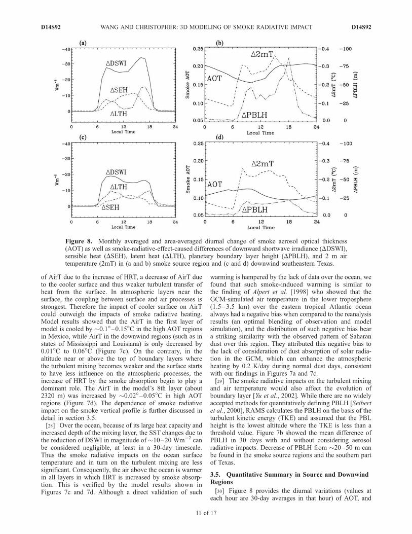
[30] Figure 8 provides the diurnal variations (values ateach hour are 30-day averages in that hour) of AOT, and

Figure 8. Monthly averaged and area-averaged diurnal change of smoke aerosol optical thickness(AOT) as well as smoke-radiative-effect-caused differences of downward shortwave irradiance (DDSWI),sensible heat (DSEH), latent heat (DLTH), planetary boundary layer height (DPBLH), and 2 m airtemperature (2mT) in (a and b) smoke source region and (c and d) downwind southeastern Texas.


11 of 17

D14S92

changes of PBLH, 2mT, SEH, LTH, and DSWI due to thesmoke radiative impacts (hereinafter DPBLH, D2mT,DSEH, DLTH, and DDSWI) in smoke source regions(Figures 8a and 8b) and downward regions (in southernTexas, Figures 8c and 8d). The daytime (12-hour) averageand all day (24-hour) average of these quantities aresummarized in Table 2. Except AOT that shows about±12% changes between day and night, other quantities aremostly pronounced during the daytime. Hereinafter in thefollowing analysis, all the averages are daytime averages.[31] Results indicate that smoke AOT is about 0.18 in the

source region, and decreases to 0.09 in the downwindregion. The area-averaged AOT has a distinct diurnalvariation of 24% (±12% from the mean) but oppositepatterns in smoke source region and the downwind regions.In source region, Figure 8b showed that the largest AOToccurs in the early afternoon (1500�1600 LT) while min-imum AOT is in the morning (0800�0900 LT), consistentwith previous findings from satellite observations [Prins etal., 1998] and ground-based observation [Eck et al., 2003].In contrast, AOT in downwind regions has maximum(minimum) value in the morning (early afternoon). Themechanism for this opposite diurnal variation pattern is notclear, although the smoke transport time from the source toTexas could shift the phase of diurnal variation.[32] Consistent with AOT diurnal variations, DSWI in

smoke source region is larger during the afternoon thanin the morning, contrary to that in the downwind regions. Inboth regions, DSWI shows two peaks, one at �0800 LT andanother is around 1600 LT. This is largely due to the solarzenith angle effect. On one hand, the total incoming solarenergy at the TOA is a function of cosine of solar zenithangle, and has maximum values during local noon. On theother hand, the AOT along the slant path is enhanced by thecosine of solar zenith angle, which means that the actualAOT that attenuates the sunlight reaches maximum valuesnear the sun set. Because of these two competing factors,DDSWI at the surface induced by the same AOT reaches themaximum value when solar zenith angle is around 60�[Christopher et al., 2003; Russell et al., 1997]. In daytime(12-hour) average, the DSWI at the surface is decreased by22.5 Wm�2 in the smoke source region, and 15.8 Wm�2 inthe downwind regions.[33] Compared to DDSWI, the change of latent heat

(DLTH) shows similar patterns but smaller values. Duringthe tropical dry season, the relative humidity near thesurface in the smoke source region is lower than that inthe smoke downwind region. As a consequence, the impactof DDSWI on the DLTH is larger in smoke downwindregion. About half of DDSWI goes to the DLTH in thedownwind southern Texas regions, while in the smoke

source region, that ratio is about 0.3 (Table 2). Indeed,DLTH is decreased by about 1.7 Wm�2 larger in downwindregions. On the other hand, DSEH mainly relies on thedifference of air temperature and surface temperature, andtherefore its diurnal pattern to some extent should follow thevariations of diurnal temperature. In daytime averages,DSEH is about �6.2 Wm�2 and �4.7 Wm�2 in smokesource and downwind regions, respectively, both showingmaximum in the early afternoon time (1300–1500 LT,Figures 8a and 8c).[34] The surface energy budget is balanced by the

DDSWI, DLTH, and DSEH as well as the change of long-wave (LW) radiation or temperature at the surface.Figures 8b and 8d showed that the D2mT has a similardiurnal variation to DDSWI with dual peaks in the earlymorning and late afternoon, implying that the change of LWis closely responded to the DDSWI in order to achieve asurface energy balance. They also showed that the atmo-spheric response to the aerosol radiative impacts has adistinct diurnal cycle. Depending on the solar zenith angles,the maximum decrease of 2mT can be as high as 0.35�C and0.28�C in smoke source and downwind regions, respectively.On an average, D2mT is decreased by 0.28�C near thesource, and about 0.20�C in the downwind region. Becausethe decrease of 2mT is much larger in the daytime than innight time, it is expected that the DTR (maximum 2mT �minimum 2mT) is reduced by the smoke radiative effects.Our calculation showed that maximum 2mT and minimum2mT are reduced respectively by 0.46�C and 0.15�C in thesmoke source region, larger than 0.31�C and 0.05�C in thedown region (Table 2). Overall, DTR is reduced by 0.31�Cand 0.26�C in the smoke source region and southern Texas,respectively.[35] The diurnal variation of DPBLH has a one to two

hour lag behind the temporal variations of DDSWI andD2mT (Figures 8b and 8d). This is because the response ofDPBLH to the decrease of 2mT involves the turbulentmixing process in the boundary layer. Thus the impact ofthe decreased heat flux can only be reflected 1�2 hourslater on the change of DPBLH. In average, the DPBLH isabout �41 m in the source and �17.2 m in the downwindregions (Table 2). Previous studies [Yu et al., 2002;Feingold et al., 2005] showed that for the same amountof AOT, the aerosol radiative effect on the PBLH alsohighly depends on the aerosol single scattering albedo(SSA) and the aerosol vertical distribution. For the moder-ately absorbing aerosols with SSA of 0.9 (the value used inthis study), the PBLH is slightly decreased when the aerosollayer is in the lower PBL (e.g., within 1 km), and can besignificantly decreased if the aerosols layer is above thePBL [Yu et al., 2002]. However, for strong absorbing

Table 2. Change of Surface Energy Budget Caused by Smoke Aerosols in the Smoke Source Region and Downwind Regionsa

AOT DDSWI, Wm�2 DLTH, Wm�2 DSEH,Wm�2 D2mT, �C DPBLH, m DMin2mT, �C DMax2mT, �C

Source regionDaytime average 0.18 �22.5 �6.2 �6.2 �0.28 �41 �0.15 �0.4624-hour average 0.18 �11.8 �3.1 �3.1 �0.21 �25 �0.15 �0.46

Downwind regionDaytime average 0.10 �15.8 �7.9 �4.7 �0.20 �17.2 �0.05 �0.3124-hour average 0.10 �7.9 �3.8 �2.8 �0.15 �11.6 �0.05 �0.31aSee text for the meanings of each acronym.


12 of 17

D14S92

aerosols (SSA = 0.8), PBLH is indeed increased when theaerosol layer is within 1 km above the surface [Yu et al.,2002]. It is important to note that these studies generallyassumed a well-mixed and time-independent aerosol profilein their simulations, hence caution must be exercised tocompare these studies with our simulations in which thesmoke profiles are modeled at each time step andare amendable to the influence of diurnal variation offire emission, ambient meteorological condition and thelarge-scale synoptic systems.[36] For instance, during local morning (say 0300 LT or

0800 LT), the smoke mass is mainly located near the surfacein the shallow boundary layer, and decreases rapidly withheight (Figure 9), because the fire emission is minimal andturbulence mixing is weak during this time period. However,as the time progresses, the stronger turbulence mixingtogether with the increased fire activities start to buildup a well-mixed smoke distribution, first within about500 m in local noon, and then within more than 1 kmat 1700 LT (Figure 9). As such, the column burden ofsmoke mass increases rapidly after the fire activity starts inthe late morning and achieves maximum values in the laterafternoon, but the surface smoke concentration has themaximum in the night. Consequently, during the night(e.g., 0300 LT), the air temperature differences betweenSMKRAD and NSMKRAD simulations (DAirT) is nega-tive with small magnitude and only appears near thesurface (Figure 9), because this difference is due to theresidual effect of DAirT in the daytime. As the sun rises(at 0800 LT), the DAirT starts to increase (e.g., morenegative or cooler) near the surface, but become positive(e.g., warming) above the PBL, consistent with Yu et al

[2002]. During the local noon and later afternoon, thiswarming continues to increase in the upper PBLH, and asPBL increases, the layer with the maximum warming alsogrows upward (Figure 9). In contrast, the cooling (negativeDAirT) continues to remain nearly constant in the lowerPBL. The critical layer at which the DAirT shifts fromnegative to positive is near 200 m during the night, andincreases to 700 m at 0500 LT. Such smoke feedbackson temperature profile enhance the atmospheric stabilityin the PBL, and as a result, more smoke mass will betrapped near the surface in SMKRAD case than that inNSMKRAD case. Although this overall smoke impact onPBLH showed in our simulation is consistent with Yu etal [2002], we learned from Figure 9 that the smokevertical profile (both shape and magnitude) can varysignificantly with the PBL process and the diurnal vari-ation of smoke emission. Hence the results from thosesimulations with constant and well-mixed smoke profileneed to be carefully scrutinized, particularly during theeddy simulation of aerosol-cloud interactions [Feingold etal., 2005].

3.6. Smoke Radiative Feedbacks and theImplications for Air Quality Studies

[37] Since the smoke radiative effects can result inmeasurable changes of surface energy budget and turbulentmixing in the PBL, one would expect to find differences insmoke distribution between the NSMKRAD and SMKRADcases. Figure 7e shows that the difference of 30-day 24-houraveraged AOT in NSMKRAD and SMKRAD cases is about0.02�0.03 in high AOT regions, and negligible in otherregions. Because AOT is a column quantity, to explain AOTdifferences, it is meaningful to first examine the differenceof smoke mass distribution in different vertical layers(Figure 7f). The smoke mass concentration in the modelfirst layer above the surface is higher in the SMKRAD casethan in the NSMKRAD case (Figure 7f). This indicates thatmore smoke is trapped in the lower PBL near the surfacebecause of the weaker turbulence mixing and lower PBLHin the SMKRAD case. Compared to NSMKRAD case, anincrease of smoke concentration by 1–3 mgm�3 inSMKRAD case can be found in several lower atmosphericlayers (up to 800 m) over the two high smoke AOT regions(Figure 7f). In contrast, the negative difference of smokeconcentration (e.g., smaller smoke concentration in theSMKRAD case) can be found in several upper atmosphericlayers (800–2000 m, figures not shown). This is because ofweaker turbulent mixing in the SMKRAD that is lessefficient in transporting smoke particles to the upper levels.In summary, the AOT and smoke concentration differencesin the SMKRAD and NSMKRAD cases are measurable andpresumably, results from SMKRAD should be more repre-sentative of real atmosphere, since SMKRAD incorporatesmore complete physics (e.g., smoke radiative impacts).However, the validation of this conclusion is still difficultbecause of the lack of accurate chemical speciation mea-surements in the study region. Since relative humidity isusually higher in the lower PBL than in upper PBL,hygroscopic effect is more pronounced in the lower PBL.For the same amount of smoke mass, larger AOT would beexpected if more smoke is located in the lower PBL (than in

Figure 9. Vertical distribution of (left) smoke massconcentration (SMC) in SMKRAD case and (right) thesmoke-radiative-effect-caused difference of air temperature(DAirT = AirTSMKRAD � AirTNSMKRAD) averaged in thesmoke source region in 30 days for four different local timeperiods (short-dashed line, 0300 LT; solid line, 0800 LT,long-dashed line, local noon; and dot-dashed line, 1700 LT).The profile of DAirT = 0 is shown as dotted line.


13 of 17

D14S92

the upper layer). This explains why SMKRAD case has arelative larger AOT than NSMKRAD case (Figure 7e).[38] The above investigation only focused on 30-day

averages. An interesting question to pose is if the impor-tance of smoke radiative impacts and feedbacks are neces-sary for consideration in air quality modeling that focuseson smaller timescales (hourly to daily). Previous theoreticalstudies [Park et al., 2001] and observations [Taubman et al.,2004] have indicated that aerosol direct radiative effectshave an important implication for photochemical processessuch as ozone formation. The photons reflected by thesmoke layer can result in more ozone formation above thesmoke layer, yet less ozone is produced beneath the smokelayer where the amount of photons is reduced by the smokeradiative extinction [Dickerson et al., 1997]. It was alsoobserved and numerically verified in the current study thatsmoke radiative effects increase the atmospheric stability,which in turn traps more smoke particles in the lower PBLnear the surface [e.g., Robock, 1988; Taubman et al., 2004].On the basis of the above observations as well as previous1D theoretical analysis and current 3D simulations, it istherefore clear that in principle, the (smoke) aerosol radia-

tive impacts should be considered in air quality modeling,although whether the model uncertainty itself would out-weigh aerosol radiative impacts is another issue. Recently,using data collected during the Nashville southern oxidantsstudies, Zamora et al. [2003] demonstrated the need forincorporating aerosol radiative impacts in the MM5 modelsto produce the realistic radiative irradiance, temperaturefields and PBL parameters that drive the air quality models.The aerosol radiation and transport components are alsonow being integrated into the WRF chemistry models(WRF-CHEM) [Grell et al., 2004]. In this study, with our3D simulations, we further found that the coupling betweenthe smoke radiative impacts and atmospheric dynamics hassignificant implications for the air quality modeling.[39] Figure 10 shows the smoke mass distribution in

different model layers (Figures 10a–10c) and smoke massdifference between SMKRAD and NSMKRAD in theselayers (Figure 10d–10f) on 10 May 2003. Also shown is thecolor-coded PM2.5 air quality category in various PM2.5

observation stations in the SEUS on this day. The regionwith high smoke concentration matches well with areas thatare in the unhealthy air quality categories. Of particular

Figure 10. (a–c) Distribution of smoke mass concentration at model third, eighth and eleventh layersabove the surface (indicated as L3, L8 and L11 at the bottom right of each plot, respectively) at 1500 UTC(1000 LT) on 10 May 2003. The results are from SMKRAD experiment. Also overlaid is the geopotentialheight (in unit of 10 m) at 850 mb, 700 mb, and 500 mb, the pressure levels that are close to L3, L8, andL11, respectively. Color-coded dots in Figure 10a indicate the air quality category in different EPA PM2.5

measurement stations [Wang et al., 2006]. (d–f) Differences of smoke mass concentration betweenSMKRAD and NSMKRAD simulations at aforementioned layers, respectively.


14 of 17

D14S92

interest is a narrow south-north belt from southeastern Texasto central Oklahoma, where all PM2.5 stations indicated anunhealthy air quality category (Figure 10a). Interestingly,this is also the zone which shows the large smoke massdifference between SMKRAD and NSMKRAD. Positivesmoke mass difference is found in the lower boundary layer(Figure 10d), which is expected (because of the aforemen-tioned smoke radiative feedbacks). However, what is unex-pected is that not all upper PBLs exhibit the negativedifference of smoke mass concentration (Figures 10e and10f). Indeed, the negative difference only exists in thesmoke source region and over the Gulf of Mexico(Figures 10e and 10f). So what is the reason for the positivedifference of smoke mass concentration in the SEUS inupper layers (Figures 10e and 10f)? Our 3D animations (notshown) indicated that the air mass in the upper layers overthe SEUS originates from the lower boundary layer in thesmoke source region. Because of smoke radiative feed-backs, the smoke concentration is higher in SMKRAD case.Under the southerly flow of a high pressure system centeredover the Gulf of Mexico (Figures 10a–10c), this smokelayer with higher concentration of smoke particles wasmaintained in the nocturnal boundary layer during itstransport to the southern Texas. When it moved northwardand started to be in the front of a trough in southern Texas, itwas uplifted under the influence of the low-level conver-gence and upward motion caused by this trough(Figures 10a–10c). Thus positive difference of smoke massconcentration is still maintained in the SMKRAD andNSMKRAD cases, even after the long-range transport. Thedifference of smoke mass concentration is about 5% (or1.5 mgm�3) in lower level, and about 10% in the upper level(figure not shown). Therefore the smoke radiative impacts,when coupled with favorable dynamical conditions, mighthave important implications for air quality modeling andother related studies such as cloud-aerosol interaction.

4. Discussion and Conclusion

[40] Using a coupled aerosol-radiation-meteorologymodel, we have quantified the direct radiative impacts ofCentral American biomass burning smoke aerosols on thesurface energy budget, air temperature, and atmosphericboundary layer processes. Unlike previous 1D theoreticalanalysis [e.g., Atwater, 1971a, 1971b; Bergstrom, 1973;Ackerman, 1977; Carlson and Benjamin, 1980; Yu et al.,2002] or the investigations using regional climate models[Chung and Zhang, 2004; Davison et al., 2004], this studybenefits from the assimilation of GOES-derived hourlysmoke emission, and therefore realistically simulates thehorizontal and vertical distribution of smoke and smokeradiative impacts. The diurnal change of smoke AOT (withpeak value in later afternoon) in the source region issuccessfully simulated in the RAMS-AROMA. Consistencyis also found between the model and in situ measurementson the temporal evolution of AOT in the downwind regions.Our limited validation showed the improvement in simulat-ing the 2mT by incorporating the smoke radiative impacts inthe model.[41] Quantitatively, we found that smoke AOT in the

source region is 0.18 (in 30-day 24-hour average), twotimes larger than that in the downwind region. However, the

reduction of DSWI, SEH, LTH, and PBLH in the source anddownwind regions are not proportional to their AOTamount, because of the difference in solar zenith angles,relative humidity, and surface characteristics (e.g., albedo,soil moisture, etc). In particular, the changes of 2mT andDTR in the source regions are 0.21�C and 0.31�C, respec-tively; only slightly larger than 0.15�C and 0.26�C in thedownwind Texas region. More importantly, we showed thatthe smoke radiative impacts enhance the atmospheric sta-bility by reducing (increasing) the temperature near thesurface (in upper boundary layer), and result in favorablemechanisms to have more smoke aerosols trapped in thelower PBL. However, this is not the case for over the oceansurface that has a large heat capacity and deep mixingdepth, which make it less sensitive thereby resulting inminimal response to the reduction of DSWI by smoke aero-sols, at least on short-term scales. Over the oceanwe found thatsmoke absorption results in an increase of temperature in bothlower and upper boundary layers. These smoke radiativefeedbacks, when coupled with dynamical processes, mighthave important implications for air quality modeling. Indeed,aerosol-radiation-meteorology coupling is identified by theU.S. weather research program as one of priorities for theimproving the air quality modeling [Dabberdt et al., 2004].This study showed that assimilating the satellite-derived hightemporal resolution emission products into meteorologicalmodels (such as in RAMS-AROMA) provides a feasiblemethodology toward that direction.[42] Since smoke direct radiative impacts on the surface

energy budget and atmospheric temperature profile are notnegligible, they might also produce feedback on the evap-oration process, cloud formation as well as precipitationdistribution [Menon et al., 2002]. However, current simu-lation of precipitation and cloud formation in GCMs andmost meteorological models still highly depends on thecloud parameterization scheme that needs further improve-ment. Recently, the explicit modeling of cloud microphys-ical processes has showed advances in pursing the linkageof aerosol to the cloud formation processes [Ackerman etal., 2000; Feingold et al., 2001]. We are planning toconduct further studies about the smoke impacts on thecloud and precipitation by developing the size-resolvedsmoke transportation schemes as well as using explicitcloud microphysics schemes [Meyers et al., 1997] inRAMS-AROMA.

[43] Acknowledgments. This research was supported by NASA’sRadiation Sciences, Interdisciplinary sciences (FLAMBE) and ACMAPprograms. J. Wang was supported by the NASA Earth System ScienceGraduate Fellowship. While in Harvard, J. Wang was supported by theNOAA Postdoctoral Fellowship Program in Climate and Global Changeunder the administration of UCAR visiting scientist program. We aregrateful to Udaysankar Nair for his constructive comments while writingthis manuscript and Jerry Harrington for providing the data of cloudradiative properties in RAMS. We thank Jeffrey Reid and Elaine Prinsfor the fire and smoke emission data and NASA Goddard DAAC for theMODIS data. The NIFMR AOT and solar irradiance data were obtainedfrom the DOE ARM program, and we are thankful to Joseph Michalsky andChuck Long for their guidance in using the data. We also thank twoanonymous reviewers for their suggestions that resulted in Figure 9.

ReferencesAckerman, A. S., O. B. Toon, D. E. Stevens, A. J. Heymsfield,V. Ramanathan, and E. J. Welton (2000), Reduction of tropical cloudinessby soot, Science, 288, 1042–1047.


15 of 17

D14S92

Ackerman, S. A., and S. K. Cox (1982), The Saudi Arabian heat low:Aerosol distributions and thermodynamics structure, J. Geophys. Res.,87, 8991–9002.

Ackerman, T. (1977), A model of the effect of aerosols on urban climateswith particular application to the Los Angeles Basin, J. Atmos. Sci., 34,531–547.

Alpert, P., Y. J. Kaufman, Y. Shay-El, D. Tanre, A. D. Silva, S. Schubert,and J. H. Joseph (1998), Quantification of dust-forced heating of thelower troposphere, Nature, 395, 367–370.

Andrews, E., P. J. Sheridan, J. A. Ogren, and R. Ferrare (2004), In situaerosol profiles over the Southern Great Plains cloud and radiation testbed site: 1. Aerosol optical properties, J. Geophys. Res., 109, D06208,doi:10.1029/2003JD004025.

Atwater, M. A. (1971a), Radiative effects of pollutants in the atmosphericboundary layer, J. Atmos. Sci., 28, 1367–1373.

Atwater, M. A. (1971b), The radiation budget for polluted layers of theurban environment, J. Appl. Meteorol., 10, 205–214.

Bergstrom, R. (1973), Modeling of the effects of gaseous and particulatepollutants in the urban atmosphere. Part I: Thermal structure, J. Appl.Meteorol., 12, 901–902.

Carlson, T. N., and S. G. Benjamin (1980), Radiative heating rate of Sahar-an dust, J. Atmos. Sci., 37, 193–213.

Carmichael, G. R., et al. (2003), Regional-scale chemical transport model-ing in support of the analysis of observations obtained during theTRACE-P experiment, J. Geophys. Res., 108(D21), 8823, doi:10.1029/2002JD003117.

Cautenet, G., M. Legrand, S. Cautenet, B. Bonnel, and G. Brogniez (1992),Thermal impact of Saharan dust over land. Part I: Simulation, J. Appl.Meteorol., 31, 166–180.

Chang, H., and T. T. Charalampopoulos (1990), Determination of the wa-velength dependences of refractive indices of flame soot, Proc. R. Soc.London, Ser A., 430, 577–591.

Chen, S.-J., Y.-H. Kuo, W. Ming, and H. Ying (1995), The effect of dustradiative heating on low-level frontogenesis, J. Atmos. Sci., 52, 1414–1420.

Chin, M., P. Ginoux, S. Kinne, O. Torres, B. N. Holben, B. N. Duncan,R. V. Martin, J. A. Logan, A. Higurashi, and T. Nakajima (2002), Tropo-spheric aerosol optical thickness from the GOCART model and compar-isons with satellite and Sun photometer measurements, J. Atmos. Sci., 59,461–483.

Chin, M., A. Chu, R. Levy, L. Remer, Y. Kaufman, B. Holben, T. Eck,P. Ginoux, and Q. Gao (2004), Aerosol distribution in the NorthernHemisphere during ACE-Asia: Results from global model, satelliteobservations, and Sun photometer measurements, J. Geophys. Res.,109, D23S90, doi:10.1029/2004JD004829.

Christopher, S. A., and J. Zhang (2002), Daytime variation of shortwavedirect radiative forcing of biomass burning aerosols from GOES 8 im-ager, J. Atmos. Sci., 59, 681–691.

Christopher, S. A., X. Li, R. M. Welch, P. V. Hobbs, J. S. Reid, and T. F.Eck (2000), Estimation of downward and top-of-atmosphere shortwaveirradiances in biomass burning regions during SCAR-B, J. Appl. Meteor-ol., 39, 1742–1753.

Christopher, S. A., J. Wang, Q. Ji, and S. Tsay (2003), Estimation of diurnalshortwave dust aerosol radiative forcing during PRIDE, J. Geophys. Res.,108(D19), 8596, doi:10.1029/2002JD002787.

Chung, C. E., and G. J. Zhang (2004), Impact of absorbing aerosol onprecipitation: Dynamic aspects in association with convective availablepotential energy and convective parameterization closure and dependenceon aerosol heating profile, J. Geophys. Res., 109, D22103, doi:10.1029/2004JD004726.

Colarco, P. R., M. R. Schoeberl, B. G. Doddridge, L. T. Marufu, O. Torres,and E. J. Welton (2004), Transport of smoke from Canadian forest fires tothe surface near Washington, D.C.: Injection height, entrainment, andoptical properties, J. Geophys. Res., 109, D06203, doi:10.1029/2003JD004248.

Cotton, W. R., et al. (2003), RAMS 2001: Current status and future direc-tions, Meteorol. Atmos. Phys., 82, 5–29.

Crutzen, P. J., and M. O. Andreae (1990), Biomass burning in the tropics:Impact on atmospheric chemistry and biogeochemical cycles, Science,250, 1669–1678.

Crutzen, P. J., L. E. Heidt, J. P. Krasnec, W. H. Pollock, and W. Seiler(1979), Biomass burning as a source of atmospheric gases CO, H2, N2O,NO, CH3Cl and COS, Nature, 282, 253–256.

Dabberdt, W. F., et al. (2004), Meteorological research needs for improvedair quality forecasting, report of the 11th prospectus development team ofthe U.S. weather research program, Bull. Am. Meteorol. Soc., 85, 563–586, doi:10.1175/BAMS-85-4-563.

Davison, P. S., D. L. Roberts, R. T. Arnold, andR.N. Colvile (2004), Estimat-ing the direct radiative forcing due to haze from the 1997 forest fires inIndonesia, J. Geophys. Res., 109, D10207, doi:10.1029/2003JD004264.

Dickerson, R. R., S. Kondragunta, G. Stenchikov, K. L. Civerolo,B. G. Doddridge, and B. N. Holben (1997), The impact of aerosolson solar ultraviolet radiation and photochemical smog, Science, 278,827–830.

Eck, T. F., et al. (2003), Variability of biomass burning aerosol opticalcharacteristics in southern Africa during the SAFARI 2000 dry seasoncampaign and a comparison of single scattering albedo estimates fromradiometric measurements, J. Geophys. Res., 108(D13), 8477,doi:10.1029/2002JD002321.

Feingold, G., L. A. Remer, J. Ramaprasad, and Y. J. Kaufman (2001),Analysis of smoke impact on clouds in Brazilian biomass burning re-gions: An extension of Twomey’s approach, J. Geophys. Res., 106,22,907–22,922.

Feingold, G., H. Jiang, and J. Y. Harrington (2005), On smoke suppressionof clouds in Amazonia, Geophys. Res. Lett., 32, L02804, doi:10.1029/2004GL021369.

Fu, Q., and K. N. Liou (1993), Parameterization of the radiative propertiesof cirrus clouds, J. Atmos. Sci., 50, 2008–2025.

Grell, G., J. Dudhia, and D. Stauffer (1995), A description of the Fifth-Generation Penn State/NCAR Mesoscale Model (MM5), NCAR/TN-398+STR, 122 pp., Natl. Cent. for Atmos. Res., Boulder, Colo.

Grell, G. A., S. E. Penkham, R. Schmitz, and S. A. Mckeen (2004), Fullycoupled ‘‘online’’ chemistry with the WRF model, paper presented atSixth Conference on Atmospheric Chemistry, Air Quality in Megacitites,Am. Meteorol. Soc., Seattle, Wash.

Harrington, J. Y., and P. Q. Olsson (2001), A method for the parameteriza-tion of cloud optical properties in bulk and bin microphysical models.Implications for arctic cloudy boundary layers, Atmos. Res., 57, 51–80.

Ichoku, C., L. A. Remer, and T. F. Eck (2005), Quantitative evaluation andintercomparison of morning and afternoon Moderate Resolution ImagingSpectroradiometer (MODIS) aerosol measurements from Terra and Aqua,J. Geophys. Res., 110, D10S03, doi:10.1029/2004JD004987.

Intergovernmental Panel on Climate Change (2001), Climate Change 2001:The Scientific Basis—Contribution of Working Group I to the Third As-sessment Report of the Intergovernmental Panel on Climate Change, edi-ted by J. T. Houghton et al., 881 pp., Cambridge Univ. Press, New York.

Jacobson, M. Z. (2001), Strong radiative heating due to the mixing state ofblack carbon in atmospheric aerosols, Nature, 409, 695–697.

Kalnay, E., et al. (1996), The NCEP/NCAR 40-year reanalysis project, Bull.Am. Meteorol. Soc., 77, 437–471.

Kaufman, Y. J., et al. (1998), The Smoke, Clouds and Radiation Experimentin Brazil (SCAR-B), J. Geophys. Res., 103, 31,783–31,808.

Koren, I., Y. J. Kaufman, L. A. Remer, and J. V. Martins (2004), Measure-ment of the effect of Amazon smoke on inhabitation of cloud formation,Science, 303, 1342–1345.

Kotchenruther, R. A., and P. V. Hobbs (1998), Humidification factors ofaerosols from biomass burning in Brazil, J. Geophys. Res., 103, 32,081–32,089.

Liousse, C., J. E. Penner, C. C. Chuang, J. J. Walton, and H. Eddleman(1996), A global three-dimensional model study of carbonaceous aero-sols, J. Geophys. Res., 101, 19,441–19,432.

Long, C. N., and T. A. Ackerman (2000), Identification of clear skies frombroadband pyranometer measurements and calculation of downwellingshortwave cloud effects, J. Geophys. Res., 105, 15,609–15,626.

Long, C. N., and K. L. Gaustad (2004), The shortwave clear-sky detectionand fitting algorithm: Algorithm operational details and explanations,Tech. Rep. ARM TR-004, Atmospheric Radiation Measurement Program,U.S. Dep. of Energy, Washington, D. C. (Available at http://www.arm.gov/publications/tech_reports/arm-tr-004.pdf)

Mellor, G. L., and T. Yamada (1974), A hierarchy of turbulentclosure models for planetary boundary layers, J. Atmos. Sci., 31,1791–1806.

Menon, S., J. Hansen, L. Nazarenko, and Y. Luo (2002), Climate effect ofblack carbon aerosols in China and India, Science, 297, 2250–2252.

Meyers, M. P., R. L. Walko, J. Y. Harrington, and W. R. Cotton (1997),New RAMS cloud microphysics parameterization. Part II: The two mo-ment scheme, Atmos. Res., 45, 3–39.

Michalsky, J. J., J. A. Schlemmer, W. E. Berkheiser, J. L. Berndt, L. C.Harrison, N. S. Laulainen, N. R. Larson, and J. C. Barnard (2001), Multi-year measurements of aerosol optical thickness in the Atmospheric Ra-diation Measurement and quantitative links programs, J. Geophys. Res.,106, 12,099–12,107.

Park, R. J., G. L. Stenchikov, K. E. Pickering, R. R. Dickerson, D. J. Allen,and S. Kondragunta (2001), Regional air pollution and its radiative for-cing: Studies with a single-column chemical and radiation transport mod-el, J. Geophys. Res., 106, 28,751–28,770.

Park, R. J., D. J. Jacob, M. Chin, and R. V. Martin (2003), Sourcesof carbonaceous aerosols over the United States and implicationsfor natural visibility, J. Geophys. Res., 108(D12), 4355, doi:10.1029/2002JD003190.


16 of 17

D14S92

Pielke, R. A., R. L. Walko, J. L. Eastman, W. A. Lyons, R. A. Stocker,M. Uliasz, and C. J. Tremback (1992), A comprehensive meteorologicalmodeling system—RAMS, Meteorol. Atmos. Phys., 49, 69–91.

Penner, J. E., R. Dickinson, and C. O’Neill (1992), Effects of aerosol frombiomass burning on the global radiation budget, Science, 256, 1423–1434.

Peppler, R. A., et al. (2000), ARM southern great plains site observations ofthe smoke pall associated with the 1998 Central American fires, Bull. Am.Meteorol. Soc., 81, 2563–2592.

Prins, E. M., J. M. Feltz, W. P. Menzel, and D. E. Ward (1998), An over-view of GOES-8 diurnal fire and smoke results for SCAR-B and the 1995fire season in South America, J. Geophys. Res., 103, 31,821–31,835.

Ramanathan, V. P., J. Crutzen, J. T. Kiehl, and D. Rosenfeld (2001), Aero-sols, climate, and the hydrological cycle, Science, 294, 2119–2124.

Reid, J. S., E. M. Prins, D. L. Westphal, C. C. Schmidt, K. A. Richardson,S. A. Christopher, T. F. Eck, E. A. Reid, C. A. Curtis, and J. P. Hoffman(2004), Real-time monitoring of South American smoke particle emis-sions and transport using a coupled remote sensing/box-model approach,Geophys. Res. Lett., 31, L06107, doi:10.1029/2003GL018845.

Reid, J. S., T. F. Eck, S. A. Christopher, R. Koppmann, O. Dubovik, D. P.Eleuterio, B. N. Holben, E. A. Reid, and J. Zhang (2005), A review ofbiomass burning emissions part III: Intensive optical properties of bio-mass burning particles, Atmos. Chem. Phys., 5, 827–849.

Remer, L. A., et al. (2005), The MODIS aerosol algorithm, product, andvalidation, J. Atmos. Sci., 62, 947–973.

Robock, A. (1988), Enhancement of surface cooling due to forest firesmoke, Science, 242, 911–913.

Rogers, C. M., and K. P. Bowman (2001), Transport of smoke from theCentral American fires of 1998, J. Geophys. Res., 106, 28,357–28,368.

Russell, P. B., S. A. Kinne, and R. W. Bergstrom (1997), Aerosol climateeffects: Local radiative forcing and column closure experiments, J. Geo-phys. Res., 102, 9397–9408.

Schafer, J. S., T. F. Eck, B. N. Holben, P. Artaxo, M. A. Yamasoe, and A. S.Procopio (2002), Observed reductions of total solar irradiance by bio-mass-burning aerosols in the Brazilian Amazon and Zambian Savanna,Geophys. Res. Lett., 29(17), 1823, doi:10.1029/2001GL014309.

Seibert, P., F. Beyrich, S.-E. Gryning, S. Joffre, A. Rasmussen, andP. Tercier (2000), Review and intercomparison of operational methods forthe determination of the mixing height, Atmos. Environ., 34, 1001–1027.

Stephens, G. L. (1984), The parameterization of radiation for numericalweather prediction and climate models,Mon. Weather Rev., 12, 826–867.

Swap, R. J., H. J. Annegarn, J. T. Suttles, M. D. King, S. Platnick, J. L.Privette, and R. J. Scholes (2003), Africa burning: A thematic analysis ofthe Southern African Regional Science Initiative (SAFARI 2000),J. Geophys. Res., 108(D13), 8465, doi:10.1029/2003JD003747.

Taubman, B. F., L. T. Marufu, B. L. Vant-Hull, C. A. Piety, B. G. Doddridge,R. R. Dickerson, and Z. Li (2004), Smoke over haze: Aircraft observa-

tions of chemical and optical properties and the effects on heating ratesand stability, J. Geophys. Res., 109 , D02206, doi:10.1029/2003JD003898.

Tegen, I., P. Hollrig, M. Chin, I. Fung, D. Jacob, and J. Penner (1997),Contribution of different aerosols to the global aerosol extinction opticalthickness: Estimates from model results, J. Geophys. Res., 102, 23,895–23,915.

Twomey, S. (1977), The influence of pollution on the shortwave albedo ofclouds, J. Atmos. Sci., 34, 1149–1152.

Walko, R. L., W. R. Cotton, M. P. Meyers, and J. Y. Harrington (1995),New RAMS cloud microphysics parameterization, part I: The single-moment scheme, Atmos. Res., 38, 29–62.

Walko, R. L., et al. (2000), Coupled atmosphere-biophysics-hydrologymodels for environmental modeling, J. Appl. Meteorol., 39, 931–944.

Wang, J. (2005), Air quality and radiative impacts of long-range transportedaerosols over the southeastern United States, Ph.D. dissertation, Dep. ofAtmos. Sci., Univ. of Ala., Huntsville.

Wang, J., U. S. Nair, and S. A. Christopher (2004), GOES 8 aerosol opticalthickness assimilation in a mesoscale model: Online integration of aero-sol radiative effects, J. Geophys. Res., 109, D23203, doi:10.1029/2004JD004827.

Wang, J., S. A. Christopher, U. S. Nair, J. S. Reid, E. M. Prins, J. Szykman,and J. L. Hand (2006), Mesoscale modeling of Central American smoketransport to the United States: 1. ‘‘Top-down’’ assessment of emissionstrength and diurnal variation impacts, J. Geophys. Res., 111, D05S17,doi:10.1029/2005JD006416.

Westphal, D. L., and O. B. Toon (1991), Simulation of microphysical,radiative, and dynamical processes in a continental-scale forest smokeplume, J. Geophys. Res., 96, 22,379–22,400.

Yu, H., S. C. Liu, and R. E. Dickinson (2002), Radiative effects of aerosolson the evolution of the atmospheric boundary layer, J. Geophys. Res.,107(D12), 4142, doi:10.1029/2001JD000754.

Zamora, R. J., S. Solomon, E. G. Dutton, J. W. Bao, M. Trainer, R. W.Portmann, A. B. White, D. W. Nelson, and R. T. McNider (2003), Com-paring MM5 radiative fluxes with observations gathered during the 1995and 1999 Nashville southern oxidants studies, J. Geophys. Res., 108(D2),4050, doi:10.1029/2002JD002122.

��S. A. Christopher, Department of Atmospheric Science, University of

Alabama, 320 Sparkman Drive, Huntsville, AL 35805, USA. ([email protected])J. Wang, Division of Engineering and Applied Science, Pierce Hall,

Room G3F, Harvard University, 29 Oxford Street, Cambridge, MA 02138,USA. ([email protected])


17 of 17

D14S92

mesoscale modeling of central american smoke transport to

Documents