Mesh Reconstruction from Aerial Images for Outdoor Terrain MappingUsing Joint 2D-3D Learning

Qiaojun Feng Nikolay Atanasov

Abstract— This paper addresses outdoor terrain mappingusing overhead images obtained from an unmanned aerialvehicle. Dense depth estimation from aerial images during flightis challenging. While feature-based localization and mappingtechniques can deliver real-time odometry and sparse pointsreconstruction, a dense environment model is generally re-covered offline with significant computation and storage. Thispaper develops a joint 2D-3D learning approach to reconstructlocal meshes at each camera keyframe, which can be assembledinto a global environment model. Each local mesh is initializedfrom sparse depth measurements. We associate image featureswith the mesh vertices through camera projection and applygraph convolution to refine the mesh vertices based on joint2-D reprojected depth and 3-D mesh supervision. Quantitativeand qualitative evaluations using real aerial images show thepotential of our method to support environmental monitoringand surveillance applications.

I. INTRODUCTION

Recent advances in sensors, processors, storage and com-munication devices have set the stage for mobile robotsystems to significantly contribute in environmental mon-itoring, security and surveillance, agriculture, and manyother applications. Constructing terrain maps onboard anunmanned aerial vehicle (UAV) using online sensory datawould be very beneficial in these applications. With inertialmeasurement unit (IMU), GPS, and camera sensors, a UAVcan localize itself and incrementally reconstruct the geomet-ric structure of the traversed terrain. Near infrared camerascan additionally provide normalized difference vegetationindex measurements for vegetation assessment and semanticsegmentation can enrich the map.

This paper considers the problem of building a terrainmodel in the form of a mesh of an outdoor environmentusing a sequence of overhead RGB images obtained onboarda UAV. We assume that the UAV is running a localizationalgorithm, based on visual-inertial odometry (VIO) [1] orsimultaneous localization and mapping (SLAM) [2] , whichestimates its camera pose and the depths of a sparse set oftracked image keypoints. One approach for outdoor terrainmapping is to recover depth images at each camera viewusing dense stereo matching. The depth images can be fusedto generate a point cloud and triangulate a mesh surface.While specialized sensors and algorithms exist for real-timedense stereo matching, they are restricted to a limited depthrange, much smaller than commonly seen in aerial images.Moreover, due to the limited depth variation, the recovered

We gratefully acknowledge support from NSF NRI CNS-1830399.The authors are with the Department of Electrical and Computer En-

gineering, University of California San Diego, La Jolla, CA 92093, USA{qjfeng,natanasov}@ucsd.edu

Fig. 1: This paper develops a method for 3-D mesh reconstruction(right) from aerial RGB images and noisy sparse depth measure-ments (left) to support outdoor terrain mapping.

point cloud might not be sufficiently dense for accurate meshreconstruction. Recently, depth completion methods [3], [4]using deep learning have shown promising performance onindoor [5] and outdoor datasets [6]. However, aerial imagesare different from the ground-level RGBD datasets used totrain these algorithm. Due to the limited availability of aerialimage datasets for supervision, learning-based methods havenot yet been widely adopted for outdoor terrain mapping.

We propose a learning-based method for mesh reconstruc-tion using a single RGB image with sparse depth measure-ments. Fig. 1 shows an example input and mesh reconstruc-tion. Our main contribution is to show that depth completionand mesh reconstruction are closely related problems. In-spired by depth completion techniques, we propose a coarse-to-fine strategy, composed of initialization and refinementstages for mesh reconstruction. In the initialization stage,we use only the sparse depth measurements to fit a coarsemesh surface by minimizing a 2-D rendered depth loss. Inthe refinement stage, we leverage both the RGB image andthe sparse depth information. We extract deep convolutionalimage features and associate them with the vertices ofthe initial mesh through camera projection. The mesh issubsequently refined using a graph convolution model topredict vertex deformations that minimize a weighted 3-Dgeometric surface loss and 2-D rendered depth loss. Giventhe camera poses, we can fuse the optimized local meshesinto a global mesh model of the environment. We build anaerial image dataset with ground-truth depth, noisy sparsedepth measurements, and multiple camera trajectories basedon WHU MVS/Stereo dataset [7] and details can be foundon https://github.com/FengQiaojun/TerrainMesh.

II. RELATED WORK

Depth Completion. Predicting depth from RGB imagesenables artificial perception systems to recover 3-D environ-

ment structure [8], [9]. While depth prediction from RGBimages alone may be challenging, sparse depth measure-ments, e.g., obtained from keypoint triangulation, simplifythe problem and lead to improvements in efficiency andaccuracy [10]. Depth completion is the task of predictingdense depth images from sparse depth measurements andcorresponding RGB images. Ma et al. [3], [11] developmethods for supervised training, relying on ground truthdepth images, as well as self-supervised training, using pho-tometric error from calibrated image pairs. Chen et al. [10]pre-process sparse depth images by generating a EuclideanDistance Transform of the depth sample locations and anearest-neighbor depth fill map. The authors propose a multi-scale deep network that treats depth completion as residualprediction with respect to the nearest-neighbor depth fillmaps. Chen et al. [4] design a 2-D convolution branch toprocess stacked RGB and sparse depth images and a 3-D convolution branch to process point clouds and fuse theoutputs of the two branches.Mesh Reconstruction. Online terrain mapping requires ef-ficient storage and updates of a 3-D surface model. Storingdense depth information from aerial images requires signifi-cant memory and subsequent model reconstruction. Explicitsurface representations, e.g., based on polygon meshes, maybe quite memory and computationally efficient but theirvertices and faces need to be optimized to fit the environ-ment geometry. FLaME [12] performs non-local variationaloptimization over a time-varying Delaunay graph to obtaina real-time inverse-depth mesh of the environment. TerrianFusion [13] performs real-time terrain mapping by generatingdigital surface model (DSM) meshes at selected keyframes.It converts the local meshes into grid-maps and merges themusing multi-band fusion. Pixel2Mesh [14] treats a mesh as agraph and applies graph convolution [15] for vertex featureextraction and graph unpooling to subdivide the mesh fordetailed refinement. Mesh R-CNN [16] simultaneously de-tects objects and reconstructs their 3-D mesh shape. A coarsevoxel representation is predicted first and then converted intoa mesh for refinement.

Our setting differs from existing work because aerial im-ages cover large regions with significantly more subtle depthvariation compared to indoor or outdoor ground settings. Ourapproach uses the same inputs as a depth completion problembut recovers a 3-D mesh model, which provides smootherdepth estimates with fewer parameters (only vertices andfaces) compared to dense depth prediction. Instead of relyingon a priori known object categories, our method provideswhole image mesh reconstruction.

III. PROBLEM FORMULATION

Consider a UAV equipped with a camera, whose positionpk ∈ R3 and orientation Rk ∈ SO(3) are estimatedat discrete time steps k by a VIO or SLAM localizationalgorithm. Denote the RGB images corresponding to thediscrete-time keyframes by Ik. Obtaining dense depth imagesduring outdoor flight is challenging but it is common forlocalization algorithms to track and estimate the depth of a

Fig. 2: Loss function illustration: `2 compares a depth image D torendered mesh depth ρ(M); `3 compares a mesh M to an elevatedmesh MD obtained from a depth image D.

sparse set of image feature points. Let D∗k denote the denseground-truth depth image, which is unknown during real-time operation. Let Dk be a sparse matrix that containsestimated depths at the image feature locations and zeroseverywhere else. Our goal is to construct an explicit modelof the camera view at time k using a 3-D triangle meshMk := (Vk, Ek,Fk), where Vk ∈ Rnk×3 are the vertexcoordinates in the camera frame, [nk] := {1, . . . , nk} is theset of vertex indices, Ek ⊆ [nk] × [nk] are the edges, andFk ⊆ [nk]× [nk]× [nk] are the faces.

Problem. Given a finite set of RGB images {Ik}k andcorresponding sparse depth measurements {Dk}k, define amesh reconstruction function M = f(I,D;θ) and optimizeits parameters θ to estimate the ground-truth depth {D∗k}k:

minθ

∑k

`(f(Ik,Dk;θ),D∗k) (1)

where `(M,D) is a loss function measuring the errorbetween a mesh M and a depth image D representing thesame camera view.

The choice of loss function ` is discussed in Sec. IV.We develop a machine learning approach to this problem,consisting of an offline training phase and an online meshreconstruction phase. During training, the parameters θ areoptimized using a training set D := {Ii,Di,D

∗i }i with

known ground-truth depth images. During testing, givenstreaming RGB images Ik and sparse depth measurementsDk, the optimized parameters θ∗ are used to constructmesh models Mk = f(Ik,Dk;θ∗). The local mesh Mk =(Vk, Ek,Fk) can be converted into the global frame bytransforming the vertex coordinates VkR

>k +1p>k using the

camera poses pk, Rk and multiple meshes can be assembled[17] to model the whole environment.

IV. LOSS FUNCTIONS FOR MESH RECONSTRUCTION

We propose several loss functions to measure the errorbetween a mesh M and a depth image D representing thesame camera view. Since our problem focuses on optimizingthe mesh representation M, the loss function must bedifferentiable with respect to the vertices of M.

A loss function can be defined in the 2-D image plane byrendering a depth image from M and comparing its pixelvalues to those of D. We rely on a differentiable meshrenderer [18], [19] to generate a depth image ρ(M) anddefine a 2-D loss function:

`2(M,D) :=

∑ij∈U(ρ(M),D) |ρij(M)−Dij |

|U(ρ(M),D)|, (2)

where U(ρ(M),D) is the set of pixels where both thedepth image D and the rendered depth ρ(M) have validdepth information. While `2 is a natural choice of a lossfunction in the image plane, it does not emphasize twoimportant properties for mesh reconstruction. First, since`2 only considers a region in the image plane where bothdepth images have valid information, its minimization overM may encourage the mesh M to shrink. Second, `2 doesnot emphasize regions of large depth gradient variation (e.g.,the side surface of a building), which may lead to inaccuratereconstruction of 3-D structures.

To address these limitations, we propose a supplementaryloss function, defined in the 3-D spatial domain over pointclouds PM and QD obtained from M and D, respectively:

`3(M,D) :=1

2λ(PM,QD) +

1

2λ(QD,PM), (3)

where λ is the asymmetric Chamfer point cloud distance:

λ(P,Q) :=1

|P|∑p∈P‖p− arg min

q∈Q‖p− q‖2‖2. (4)

To generate PM, we sample the faces of M uniformly.Since samples on the mesh surface can be represented usingbarycentric coordinates with respect to the mesh vertices,the loss function is differentiable with respect to the meshvertices. To generate QD, we may sample the depth imageD uniformly and project the samples to 3-D space but thiswill not generate sufficient samples in the regions of largedepth gradient variation. Instead, we first generate a pseudoground-truth meshMD by densely sampling pixel locationsin D as the mesh vertices and triangulating on the imageplane to generate faces. We then sample the surface of MD

uniformly to obtain QD.Fig. 2 illustrates the loss functions `2 and `3. We also

define two regularization terms to measure the smoothnessof M = (V, E ,F). The first is based on the Laplacianmatrix L := G −A ∈ Rn×n of M, where G is the vertexdegree matrix and A is the adjacency matrix. We define avertex regularization term based on the `2,1-norm [20] of thedegree-normalized Laplacian [21] G−1L:

`V(M) :=1

n

∥∥G−1LV∥∥

2,1. (5)

We also introduce a mesh edge regularization term to dis-courage long edges in the mesh

`E(M) :=1

|E|∑

(i,j)∈E

‖vi − vj‖2, (6)

where vi ∈ R3 are the mesh vertices. The complete lossfunction is:

`(M,D) := w2`2(M,D) + w3`3(M,D)

+ wV`V(M) + wE`E(M),(7)

where the first two terms evaluate the error between Mand D and the last two terms encourage smoothness of themesh structure. The scalars w2, w3, wV, wE allow appropri-ate weighting of the different terms in (7).

V. 2D-3D LEARNING FOR MESH RECONSTRUCTION

Inspired by depth completion techniques, we approachmesh reconstruction in two stages: initialization and refine-ment. We initialize a coarse mesh from the sparse depthmeasurements and refine it by predicting vertex residualsbased on RGB image features.

A. Mesh Initialization

Outdoor terrain structure can be viewed as a 2.5-D surfacethat is mostly flat with occasional height variations. Hence,we initialize a flat mesh and change the surface elevationbased on the sparse depth measurements. The flat mesh isinitialized with regular-grid vertices (1024 in our experi-ments) over the X-Y ground plane, orthogonal to the gravitydirection (Z axis). See Fig. 3 for an illustration. Subsequently,our mesh reconstruction approach only optimizes the meshvertices and keeps the edge and face topology fixed. Weinitialize the Z-axis vertex coordinates by solving an opti-mization problem with a weighted combination of the 2-Drendered depth loss `2 in (2) and the Laplacian loss `V in(5) as the objective function:

∆V∗ = arg min∆V

w2`2(M(V + ∆V, E ,F),D)

+ wV`V(M(V + ∆V, E ,F)).(8)

In (8), D are sparse depth measurements so the rendereddepth error is evaluated only at the sparse pixel locations.The initialized meshMint = (V+∆V∗, E ,F) is used as aninput to the mesh refinement stage.

B. Mesh Refinement

In the refinement stage, we use a learning approach toextract features from both the 2-D image and 3-D initialmesh and regress mesh vertex offsets. The ground-truth depthmaps are used for supervision.

The RGB image provides useful information for refine-ment since man-made objects have sharp vertical surfaces,while natural terrain has noisy but limited depth variation.The sparse depth measurements also provide informationabout areas with large intensity variation. Inspired by MeshR-CNN [16], we design a network that extracts features fromthe 2-D image, associates them with the 3-D vertices of theinitial mesh, and uses them to refine the vertex locations.Our network has 3 stages: feature extraction, vertex-imagefeature alignment, and vertex graph convolution.Feature Extraction. We extract features from three sources:the RGB image I, the rendered depth ρ(Mint) from theinitial mesh, and a Euclidean distance transform E(D) of the

Fig. 3: Overview of the complete mesh reconstruction architecture. In the mesh initialization stage (Sec. V-A), we use sparse depths toelevate a flat mesh from the image plane to 3-D space. In the mesh refinement stage (Sec. V-B), we combine the RGB image, the initialmesh rendered depth and the Euclidean Distance Transform from the sparse depths and extract 2-D features using ResNet-18 [22]. Thesefeatures are aligned to the initial mesh vertices using camera projection (Fig. 4). Vertex offsets are regressed using a graph convolutionnetwork (GCN) over the initial mesh. The ResNet-18 and GCN parameters are optimized jointly using the loss function in Sec. IV.

Fig. 4: Illustration of image feature to mesh vertex association.With known camera intrinsics, each mesh vertex can be projectedin uv coordinates (range [0, 1]) onto the image plane. Bilinearinterpolation is used to associate image feature maps at differentresolutions with the mesh vertices. The features across differentresolutions are concatenated to form a composite vertex feature.

sparse depth measurements D, obtained by computing theEuclidean distance to the closest valid depth measurementfor each pixel. The three images are concatenated to forma 5-channel input: C = concat(I, ρ(Mint),E(D)). We useResNet-18 [22] to extract image features. Since aerial imageshave different properties compared to ImageNet data, welearn the model weights from scratch. Four layers of featureswith different resolution and channels are extracted:

[L1,L2,L3,L4] = φ(C), (9)

where φ is the ResNet-18 model.Vertex-Image Feature Alignment. Next, we construct 3-D features for Mint by associating the mesh vertices withthe 2-D image features. This idea is inspired by Pixel2Mesh[14], which projects mesh vertices onto the image planeand extracts features at the projected coordinates. To obtainmulti-scale features, we associate the projected mesh verticeswith the intermediate layer feature maps [L1,L2,L3,L4]from (9). This vertex-image alignment step is illustratedin Fig. 4. All features with different channel numbers are

concatenated to form composite vertex features:

Vgin = galign(Mint, φ(C)), (10)

where Vgin ∈ Rn×(l1+l2+l3+l4+3) are the vertex features andli is the number of channels in feature map Li. We add the3-D vertex coordinates vi as the last 3 dimensions.Vertex Graph Convolution. The mesh can be viewed as agraph with vertex features Vgin . A graph convolution network[15], [16] is a suitable architecture to process the vertexfeatures and obtain vertex offsets ∆V that optimize theagreement of the refined mesh Mref = (Vint + ∆V, E ,F)and the ground truth depth D∗ according to the loss in (7).To capture a larger region of feature influence, we use 3layers of graph convolution g1, g2, g3 and set the final vertexfeature dimension to 64. A weight matrix W is applied onthe final 64-D feature to derive the 3-D vertex offsets:

∆V = WVgout := Wg3(g2(g1(Vgin))), (11)

where Vgout ∈ Rn×64 and ∆V ∈ Rn×3. In order to refine themesh with more details, we concatenate 3 stages of vertex-image feature alignment and graph convolution. At stage i,last stage’s refined mesh Mref

i−1 is set as the initial meshMint

i and new vertex features are extracted via vertex-imagefeature alignment and fed to new graph convolution layers.All 3 refined meshes in different stages (Mref

1 ,Mref2 ,Mref

3 )are evaluated against the ground-truth depth map D∗ usingthe loss functions defined in (7).

VI. EXPERIMENTS

This section compares several variations of our meshreconstruction approach to a baseline method on a datasetgenerated from aerial images.

A. Dataset

We build an aerial image dataset based on the WHUMVS/Stereo dataset [7]. The original dataset provides cal-ibrated RGBD images rendered from a highly accurate 3Ddigital surface model which is not publicly available. Hence,

TABLE I: Quantitative evaluation of variations of the proposed method. The SD-tri method triangulates a mesh using all the sparse depthmeasurements as vertices. The Regular-n uses the mesh with n vertices. The Initialized model constructs a mesh from the sparse depth(Sec. V-A). The RGB, RGB+RD, RGB+RD+EDT methods refine the initialized mesh (Sec. V-B), using different inputs respectively. Theloss function used by the different methods is indicated by 3D+2D (uses both `3 and `2) or 3D (uses `3 only). The second column showsthe number of available sparse depth measurements per image and indicates whether the measurements are noisy (Sec. VI-A).

ErrorMeshing SD-tri Regular-576 Regular-1024

Inputs (vert= SD) Initialized RGB+RD RGB+RD+EDT Initialized RGB RGB+RD RGB+RD RGB+RD+EDT

Loss 3D+2D 3D+2D 3D+2D 3D 3D+2D 3D+2D

`2

500 1.492 2.069 1.670 1.637 1.861 1.575 1.382 1.289 1.2521000 1.172 1.834 1.596 1.546 1.535 1.298 1.193 1.124 1.0972000 0.916 1.941 1.551 1.511 1.344 1.144 1.092 1.045 1.024

`3

500 9.815 18.278 13.438 13.763 13.799 7.242 5.412 5.647 6.3521000 6.494 17.762 12.938 13.574 11.872 5.876 4.538 4.911 5.7032000 4.649 17.130 12.483 13.506 10.859 5.131 4.069 4.477 5.291

`2

500+noise 1.865 2.294 1.809 1.768 2.155 1.828 1.571 1.486 1.4561000+noise 1.632 2.056 1.701 1.685 1.826 1.535 1.360 1.319 1.3082000+noise 1.485 1.717 1.655 1.654 1.629 1.364 1.243 1.236 1.241

`3

500+noise 19.737 18.392 12.974 13.532 14.887 8.351 6.063 6.157 6.8651000+noise 22.189 17.693 12.258 13.161 12.480 6.447 4.904 5.266 6.0752000+noise 18.545 17.256 11.856 12.988 11.147 5.452 4.343 4.793 5.620

we recover a dense point cloud from the RGBD images asa ground-truth 3D model. We generate 20 camera trajectorysequences, split into 14 for training, 2 for validation, and4 for testing. Each camera trajectory follows a sweepinggrid-pattern with 10 keyframes per row and 20 keyframesper column. The keyframes are chosen to ensure 75% rowoverlap and 80% column overlap. RGBD images with reso-lution 512×512 are rendered along each trajectory from theground-truth point cloud using PyTorch3D [19]. We obtaincamera pose estimates and sparse depth measurements Dk

for each image by applying OpenSfM [23] to four neighborimages with known camera intrinsic parameters. Small (500),medium (1000), and large (2000) number of sparse depthmeasurements are obtained from SfM per image. The resultsfrom OpenSfM are treated as the data with noise, and thenoise may come from the feature detection&matching as wellas the bundle adjustment step. We also obtain noiseless depthmeasurements with the same sparsity 2-D pattern from theground-truth depth images D∗k.

B. Implementation Details

During training, we use 1000 number of sparse depthmeasurements and the mesh vertices number is fixed to1024. The mesh initialization optimization is performed over100 iterations with the Adam optimizer [24] and weights[w2, w3, wV, wE ] = [1, 0, 0.5, 0] for the loss function in(7). The ResNet-18 and GCN parameters are optimizedjointly during the mesh refinement training using the Adamoptimizer with initial learning rate of 0.0005 for 200 epochs.The loss function in (7) with parameters [w2, w3, wV, wE ] =[3, 1, 0.5, 0.01] is used in this phase. The Chamfer distanceλ in the `3 loss term is computed using 10000 samples.

C. Results

Our experiments report the `2 error in (2) and the `3error in (3), comparing the reconstructed mesh wit. The `2emphasizes projected depth accuracy, while the `3 pay moreattention to large depth gradient region.

For comparison, we define a baseline method that triangu-lates the sparse depth measurements directly to build a mesh.

The baseline method performs Delaunay triangulation on the2-D image plane over the depth measurements and projectsthe flat mesh to 3-D using the known vertex depths. We referto the baseline method as sparse-depth-triangulation (SD-tri). Note that the baseline method uses all avaiable sparsedepth measurements (500, 1000, or 2000) and, hence, mayhas a different number of vertices from the other models.The quantitative results from the comparison are reported inTable I. Note that all the models are trained with 1024-vertexmeshes and 1000 sparse depth measurements and we directlygeneralize them on meshes with different number of verticesand different number of sparse depth measurements.

Several variations of our approach are evaluated. Wecompared three different options for the input providedto the mesh refinement stage: only the 3-channel RGBimage (RGB), the RGB image plus rendered depth fromthe initial mesh (RGB+RD, 4-channels), and the RGB im-age plus rendered depth from the initial mesh plus Eu-clidean distance transform obtained from of the sparse depthmap (RGB+RD+EDT, 5-channels). The model using RGB-only does not perform as well as the other two. TheRGB+RD+EDT model has the best performance accordingto the `2 error metric. The RGB+RD method has similarperformance in the `2 metric and smaller `3 error comparedto RGB+RD+EDT. The RGB+RD model is used to generateour qualitative results using 1024-vertex meshes because itoffers good performance according to both error metrics.

We also compare different loss function combinations fortraining the RGB+RD method. The 3D+2D loss functionreported in Table I corresponds to training with parameters[w2, w3, wV, wE ] = [3, 1, 0.5, 0.01] for the loss function in(7), while the 3D loss function, corresponds to parameters[w2, w3, wV, wE ] = [0, 1, 0.5, 0.01]. We can see that trainingwith the 3D+2D loss leads to balanced performance acorrd-ing to both the `2 and `3 metrics, while training with the 3Dloss only leads to good performance in the `3 loss but higher2-D rendering error, according to the `2 metric.

Finally, we compare the mesh reconstruction accuracywhen the sparse depth measurements are noiseless ver-

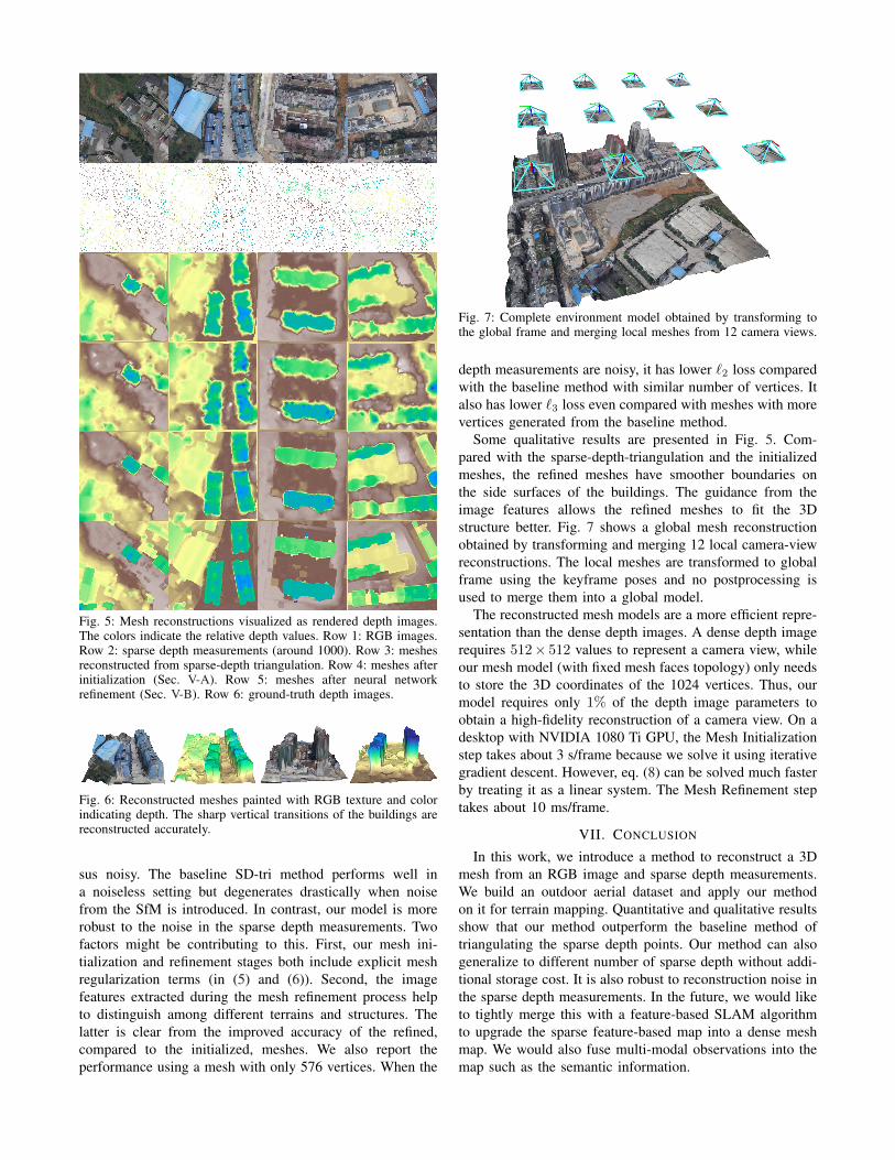
Fig. 5: Mesh reconstructions visualized as rendered depth images.The colors indicate the relative depth values. Row 1: RGB images.Row 2: sparse depth measurements (around 1000). Row 3: meshesreconstructed from sparse-depth triangulation. Row 4: meshes afterinitialization (Sec. V-A). Row 5: meshes after neural networkrefinement (Sec. V-B). Row 6: ground-truth depth images.

Fig. 6: Reconstructed meshes painted with RGB texture and colorindicating depth. The sharp vertical transitions of the buildings arereconstructed accurately.

sus noisy. The baseline SD-tri method performs well ina noiseless setting but degenerates drastically when noisefrom the SfM is introduced. In contrast, our model is morerobust to the noise in the sparse depth measurements. Twofactors might be contributing to this. First, our mesh ini-tialization and refinement stages both include explicit meshregularization terms (in (5) and (6)). Second, the imagefeatures extracted during the mesh refinement process helpto distinguish among different terrains and structures. Thelatter is clear from the improved accuracy of the refined,compared to the initialized, meshes. We also report theperformance using a mesh with only 576 vertices. When the

Fig. 7: Complete environment model obtained by transforming tothe global frame and merging local meshes from 12 camera views.

depth measurements are noisy, it has lower `2 loss comparedwith the baseline method with similar number of vertices. Italso has lower `3 loss even compared with meshes with morevertices generated from the baseline method.

Some qualitative results are presented in Fig. 5. Com-pared with the sparse-depth-triangulation and the initializedmeshes, the refined meshes have smoother boundaries onthe side surfaces of the buildings. The guidance from theimage features allows the refined meshes to fit the 3Dstructure better. Fig. 7 shows a global mesh reconstructionobtained by transforming and merging 12 local camera-viewreconstructions. The local meshes are transformed to globalframe using the keyframe poses and no postprocessing isused to merge them into a global model.

The reconstructed mesh models are a more efficient repre-sentation than the dense depth images. A dense depth imagerequires 512× 512 values to represent a camera view, whileour mesh model (with fixed mesh faces topology) only needsto store the 3D coordinates of the 1024 vertices. Thus, ourmodel requires only 1% of the depth image parameters toobtain a high-fidelity reconstruction of a camera view. On adesktop with NVIDIA 1080 Ti GPU, the Mesh Initializationstep takes about 3 s/frame because we solve it using iterativegradient descent. However, eq. (8) can be solved much fasterby treating it as a linear system. The Mesh Refinement steptakes about 10 ms/frame.

VII. CONCLUSION

In this work, we introduce a method to reconstruct a 3Dmesh from an RGB image and sparse depth measurements.We build an outdoor aerial dataset and apply our methodon it for terrain mapping. Quantitative and qualitative resultsshow that our method outperform the baseline method oftriangulating the sparse depth points. Our method can alsogeneralize to different number of sparse depth without addi-tional storage cost. It is also robust to reconstruction noise inthe sparse depth measurements. In the future, we would liketo tightly merge this with a feature-based SLAM algorithmto upgrade the sparse feature-based map into a dense meshmap. We would also fuse multi-modal observations into themap such as the semantic information.

REFERENCES

[1] T. Qin, P. Li, and S. Shen, “VINS-Mono: A Robust and VersatileMonocular Visual-Inertial State Estimator,” IEEE Transactions onRobotics, vol. 34, no. 4, pp. 1004–1020, 2018.

[2] C. Cadena, L. Carlone, H. Carrillo, Y. Latif, D. Scaramuzza, J. Neira,I. Reid, and J. J. Leonard, “Past, Present, and Future of SimultaneousLocalization and Mapping: Toward the Robust-Perception Age,” IEEETransactions on Robotics, vol. 32, no. 6, pp. 1309–1332, 2016.

[3] F. Ma and S. Karaman, “Sparse-to-Dense: Depth Prediction fromSparse Depth Samples and a Single Image,” in IEEE InternationalConference on Robotics and Automation (ICRA), 2018, pp. 4796–4803.

[4] Y. Chen, B. Yang, M. Liang, and R. Urtasun, “Learning Joint 2D-3D Representations for Depth Completion,” in 2019 IEEE/CVF Inter-national Conference on Computer Vision (ICCV), 2019, pp. 10 022–10 031.

[5] J. Sturm, N. Engelhard, F. Endres, W. Burgard, and D. Cremers, “Abenchmark for the evaluation of RGB-D SLAM systems,” in IEEE/RSJInternational Conference on Intelligent Robots and Systems, 2012, pp.573–580.

[6] A. Geiger, P. Lenz, C. Stiller, and R. Urtasun, “Vision meets robotics:The KITTI dataset,” The International Journal of Robotics Research,vol. 32, no. 11, pp. 1231–1237, 2013.

[7] J. Liu and S. Ji, “A Novel Recurrent Encoder-Decoder Structure forLarge-Scale Multi-View Stereo Reconstruction From an Open AerialDataset,” in IEEE/CVF Conference on Computer Vision and PatternRecognition (CVPR), 2020, pp. 6049–6058.

[8] C. Godard, O. M. Aodha, M. Firman, and G. Brostow, “DiggingInto Self-Supervised Monocular Depth Estimation,” in IEEE/CVFInternational Conference on Computer Vision (ICCV), 2019, pp. 3827–3837.

[9] A. Gordon, H. Li, R. Jonschkowski, and A. Angelova, “Depth FromVideos in the Wild: Unsupervised Monocular Depth Learning FromUnknown Cameras,” in IEEE/CVF International Conference on Com-puter Vision (ICCV), 2019, pp. 8976–8985.

[10] Z. Chen, V. Badrinarayanan, G. Drozdov, and A. Rabinovich, “Esti-mating Depth from RGB and Sparse Sensing,” in Computer Vision –ECCV, 2018, pp. 176–192.

[11] F. Ma, G. V. Cavalheiro, and S. Karaman, “Self-Supervised Sparse-to-Dense: Self-Supervised Depth Completion from LiDAR and Monocu-

lar Camera,” in International Conference on Robotics and Automation(ICRA), 2019, pp. 3288–3295.

[12] W. N. Greene and N. Roy, “FLaME: Fast Lightweight Mesh Esti-mation Using Variational Smoothing on Delaunay Graphs,” in IEEEInternational Conference on Computer Vision (ICCV), 2017, pp. 4696–4704.

[13] W. Wang, Y. Zhao, P. Han, P. Zhao, and S. Bu, “TerrainFusion:Real-time Digital Surface Model Reconstruction based on MonocularSLAM,” in IEEE/RSJ International Conference on Intelligent Robotsand Systems (IROS), 2019, pp. 7895–7902.

[14] N. Wang, Y. Zhang, Z. Li, Y. Fu, W. Liu, and Y.-G. Jiang,“Pixel2Mesh: Generating 3D Mesh Models from Single RGB Images,”in Computer Vision – ECCV, 2018, pp. 55–71.

[15] T. N. Kipf and M. Welling, “Semi-Supervised Classification withGraph Convolutional Networks,” in International Conference onLearning Representations (ICLR), 2017.

[16] G. Gkioxari, J. Johnson, and J. Malik, “Mesh R-CNN,” in IEEE/CVFInternational Conference on Computer Vision (ICCV), 2019, pp. 9784–9794.

[17] Y. Yu, K. Zhou, D. Xu, X. Shi, H. Bao, B. Guo, and H.-Y. Shum,“Mesh editing with poisson-based gradient field manipulation,” ACMTrans. Graph., vol. 23, no. 3, p. 644–651, Aug. 2004.

[18] S. Liu, T. Li, W. Chen, and H. Li, “A General Differentiable MeshRenderer for Image-based 3D Reasoning,” IEEE Transactions onPattern Analysis and Machine Intelligence, pp. 1–1, 2020.

[19] N. Ravi, J. Reizenstein, D. Novotny, T. Gordon, W.-Y. Lo, J. Johnson,and G. Gkioxari, “Accelerating 3D Deep Learning with PyTorch3D,”arXiv:2007.08501, 2020.

[20] F. Nie, H. Huang, X. Cai, and C. H. Ding, “Efficient and robust featureselection via joint `2,1-norms minimization,” in Advances in NeuralInformation Processing Systems 23, 2010, pp. 1813–1821.

[21] O. Sorkine, D. Cohen-Or, Y. Lipman, M. Alexa, C. Rossl, and H.-P. Seidel, “Laplacian Surface Editing,” in Proceedings of the 2004Eurographics/ACM SIGGRAPH Symposium on Geometry Processing,2004, p. 175–184.

[22] K. He, X. Zhang, S. Ren, and J. Sun, “Deep Residual Learning forImage Recognition,” in IEEE Conference on Computer Vision andPattern Recognition (CVPR), 2016, pp. 770–778.

[23] “OpenSfM,” https://github.com/mapillary/OpenSfM.[24] D. P. Kingma and J. Ba, “Adam: A method for stochastic opti-

mization,” in International Conference on Learning Representations(ICLR), 2014.