Ocean Dynamics (2012) 62:1217–1228DOI 10.1007/s10236-012-0559-z

Mesh generation in archipelagos

Arjen Douwe Terwisscha van Scheltinga ·Paul Glen Myers · Julie D. Pietrzak

Received: 12 December 2011 / Accepted: 1 June 2012 / Published online: 30 June 2012© Springer-Verlag 2012

Abstract A new mesh size field is presented that isspecifically designed for efficient meshing of highlyirregular oceanic domains: archipelagos. The new ap-proach is based on the standard mesh size field thatuses the proximity to the nearest coastline. Here, theproximities to the two nearest coastlines are used tocalculate the distance between two islands or the widthof a strait through an archipelago. The local value ofthe mesh size field is taken as the width (or distancebetween two islands) divided by the number of requiredelements across the strait (or between the islands). Thisnew mesh size fields are illustrated for three examples:(1) the Aegean Sea, (2) the Indonesian Archipelago,and (3) the Canadian Arctic Archipelago.

Keywords Unstructured meshes · Mesh generation ·Multi-scale modeling · Oceanography

Responsible Editor: Mohamed Iskandarani

This article is part of the Topical Collection on Multi-scalemodelling of coastal, shelf and global ocean dynamics

A. D. Terwisscha van Scheltinga · P. G. MyersDepartment of Atmospheric and Earth Sciences,University of Alberta, Edmonton, Alberta, Canada

J. D. PietrzakFaculteit CTIG, Technische Universiteit Delft,Delft, The Netherlands

Present Address:A. D. Terwisscha van Scheltinga (B)School of Earth Sciences, University of Bristol, Bristol, UKe-mail: gladtvs@bristol.ac.uk

1 Introduction

The world’s oceans are bounded by continents andisland coastlines, resulting in complex and irregulargeometry on many spatial scales. There are large oceanbasins bordered by the continents which have islandsin their interior. There are archipelagos, separating theocean basin and lesser bodies of water, which allowfor interbasin transports of water masses. For exam-ple, the Indonesian throughflow transports water fromthe Pacific to the Indian Ocean through the Indone-sian Archipelago and is an important component ofthe global overturning circulation (Godfrey 1996; Leeet al. 2002) and global climate system (Schneider 1998).Another example is the Canadian Arctic Archipelago(CAA). Freshwater is transported from the ArcticOcean through the CAA to the Labrador Sea and thusto the Atlantic Ocean.

For many applications, well-represented coastlinesare an essential component of ocean modeling. Tradi-tionally, ocean models are based on finite differenceschemes on structured grids (Griffies et al. 2000).The disadvantage of this approach is that representingcoastlines and geometric features like narrow straitsand small island is not straightforward. A sufficientresolution in these narrow straits, or near these small is-lands, can only be achieved by increasing the resolutionof the structured grid, greatly increasing the computa-tional overhead. The alternative, sufficient resolutionfor most of the domain and not representing smallislands or narrow straits, is computationally cheaper butdoes not represent the small-scale dynamics that mightbe important.

An unstructured mesh approach circumvents thisissue, since it has the advantage of accurately repre-

1218 Ocean Dynamics (2012) 62:1217–1228

senting complex and irregular coastlines. In addition,it allows for a spatially varying mesh resolution (e.g.,Adcroft and Marshall 1998; Legrand et al. 2006). Oneapproach to unstructured meshes is the finite elementmethod, which has been used for several decades inengineering. In the past two decades, geometrical do-mains that are used for design and finite elementsare built using computer-aided design (CAD). Mostcomplex features like machine parts or assemblies canbe easily and efficiently be dealt with by CAD. Finiteelements and unstructured meshes have been used inocean modeling (e.g., Danilov et al. 2005; Piggott et al.2007; White et al. 2008).

In generating the unstructured mesh for ocean mod-eling, first a suitable boundary has to be defined, i.e.,the boundary representation (BRep): shorelines in thehorizontal direction and bathymetry in the verticaldirection. Inadequate representation of the shorelinemay lead to problems (Pain et al. 2005; Adcroft andMarshall 1998), such as spurious stresses in case of stair-case shorelines present in structured meshes. Gormanet al. (2007) proposed a method to approximate theshorelines with polygons and polylines. Gorman et al.(2006) described an automatic procedure that builds aBRep of the geometry of the world ocean within pre-scribed accuracy. Both use the high resolution shorelinedata bases and bathymetry data.

Using mesh generation algorithms, a mesh is pro-duced from the BRep. At first, these algorithms wereadapted from classical engineering tools. The meshgeneration software of Henry and Waters (1993) wasused by Le Provost et al. (1994) to generate a meshof the world ocean used for tidal modeling. The samekind of meshes at a higher resolution was used by Lyardet al. (1994). On regional scales, Legrand et al. (2006)produced high-resolution meshes of the Great BarrierReef. For generation of meshes in coastal regions,Hagen et al. (2001) developed two algorithms, whichwere used for tidal modeling in the Gulf of Mexico.Specific algorithms were designed for the world oceanby Legrand et al. (2000), Gorman et al. (2007).

These algorithms use definitions of a local meshsize field to control the size and shape of the ele-ments. Definitions that can be used are proximity to thenearest shore, bathymetry, or various error estimates.Depending on the geometry, several fields can be usedsimultaneously. Usually, the minimum over all thesefields is taken. For example, for each coast (or groupof coastlines), a mesh size field can be defined basedon the proximity to this coastline (or group of coast-lines). For most applications, defining a small numberof these fields is sufficient. However, when dealing witharchipelagos, this becomes more difficult. Archipelagos

generally consist of a large number of islands withirregular coastlines and with a wide range of sizes. Theislands are separated by straits of different lengths andvarying widths. To obtain a mesh of sufficient resolu-tion using mesh size fields based on the proximity tothe nearest shoreline is difficult since one would needa lot of different mesh size fields in order to obtain asufficient resolution in each strait. This is computation-ally expensive and fine-tuning all these fields is laborintensive, even when only the most important straits arerefined.

Here, we propose an algorithm that automatesthe meshing generation of irregular geometries ofarchipelagos. The algorithm is designed such that itgenerates a mesh in selected areas in the archipelagowith a desired resolution. It only needs a collectionof coastlines, and no additional fine-tuning for eachshoreline in this collection is necessary, since the meshsize fields based on the proximity to the shorelinesin this collection has been replaced by a new singlemesh size field. This field only depends on the desiredresolution and the proximity to the nearest shoreline inthis collection. In addition, this field converges asymp-totically to any given background mesh field.

The paper is divided into three section. First, weoutline the procedure for constructing a boundary rep-resentation and generating a mesh. In the second sec-tion, we describe the new algorithm. In the last section,we show some examples of meshes produced by thisalgorithm.

2 Mesh generation on a sphere

In this section, we will give an overview of the proce-dures for building geometrical models of the ocean andmesh generation. A more thorough discussion is pre-sented in Lambrechts et al. (2008). The discussion hereis limited only to those topics needed for discussion inlater sections.

2.1 Geometric model

Before a mesh can be generated, a geometric model ofthe ocean must be defined. This geometric model of theocean, 2D or 3D, can be represented by its boundaryrepresentation. A curve is bounded by two points, asurface by curves and a volume by surfaces. Therefore,the model consists of model entities: 2D model surfaces,1D model edges, and 0D model vertices. Usually, aparametrization of these shapes is available and oftenis mappings.

Ocean Dynamics (2012) 62:1217–1228 1219

In this geometric model, a coastline is usually definedas a periodic curve. Though several approaches areavailable, like using a piecewise linear interpolation,here we use cubic B-splines. This allows for moreflexibility. The control points for the B-splines aretaken from the Global Self-consistent HierarchicalHigh-resolution Shorelines database (GSHHS, Wesseland Smith 1996). This is the most accurate shorelinedatabase, and is guaranteed to be self-consistent, i.e.,in this database, coastlines do not intersect. A size fieldγ (x) can be defined that gives the desired accuracy ofthe geometrical model at any point x. The GSHHS dataare coarsened by collapsing every successive point at xthat is closer than γ (x).

The are several choices for parameterizing a sphere.In oceanography, most of the time geographic or spher-ical coordinates are used. The mapping of the coor-dinate system might have some particular problems:(1) a singular point might exist, (2) one of the coordi-nates might be periodic, (3) shorelines might cross aperiodic edge, and (4) the mapping does not con-serve angles, i.e., the mapping is not conformal. Asa result, this leads to complexity in the definition ofthe geometric model. Though a conformal mappingis preferred since it conserves angles, there might beapplications where a parametrization is not conformaland anisotropic mesh has to be constructed in the para-metric plane to obtain an isotropic mesh in real space.

2.2 Local mesh size

After the boundaries have been represented by B-splines, finite element meshes can be generated on thesurfaces. Usually, the mesh generator builds elements,by adapting the mesh size field to control their size andshape. This mesh size field is a scalar function δ(x) thatdefines the optimal size of an edge at position x. For theworld oceans, some choices for the δ exist (Lambrechtset al. 2008).

The bathymetry H(x) can be taken into account byforcing the mesh to capture its variations. Since thebathymetry is usually interpolated piecewise linearly atthe mesh vertices, the first term in its error is depen-dent on the absolute maximum eigenvalue λmax of theHessian

H(x) = ∇2(

H(x)

Href

), (1)

where Href is a reference bathymetry. This leads to acriterion field f1(x) = 1/

√λmax.

In addition, the mesh can be forced to capture fora reference depth the wavelength of the gravity waves,which travel at speed

√gH, with g being acceleration

due to gravity. The length scale of a gravity waves λ isproportional to O(1/

√H). If one wave with a minimum

wavelength λmin is to be captured by N mesh sizes fora given reference bathymetry Href, a criterion functionf2(x) can be designed as

f2(x) = λmin

N

√Href

H(x). (2)

Coastlines need to be resolved well, in order tocapture small-scale phenomena. The mesh size shoulddecrease towards the coastline. As such, the functionf3(x) can be defined that measures the proximity to thenearest coastline:

f3(x) = d(x), (3)

where d(x) is the distance to the nearest shoreline.It is possible to add other size fields, such as error

estimates dependent on the finite element solution.Also, to produce a mesh in parametric space with rightsizing in real space, suitable mesh size fields should bedefined in parametric space.

The mesh size field δi(x) is now computed from thecriterion field fi(x) by assuming δi(x) to be a linearfunction of fi(x) within a refinement zone. Define thedesired small and large mesh sizes δ small

i and δlargei and

the zone of refinement defined by the criterion fieldvalues f min

i and f maxi . The linear function αi(x) in the

zone of refinement is given by

αi(x) =

⎧⎪⎪⎪⎪⎨⎪⎪⎪⎪⎩

0 if fi(x) ≤ f mini

fi(x) − f mini

f maxi − f min

i

if f mini < fi(x) < f max

i

1 if fi(x) ≥ f maxi

(4)

The mesh size field δi(x) follows from

δi(x) = δ smalli + αi(x)

(δ

largei − δ small

i

). (5)

The final mesh size field is taken to be the minimumof all size fields: δ(x) = min(δ1(x), δ2(x), · · · ). In thispaper, we will focus on defining a criterion functionf and mesh size function δ that refines the mesh innarrow straits. As such, we will not take into accountbathymetry, though it can be taken into account by in-cluding a mesh size field based on the bathymetry to theminimum operator. Before discussing this refinement,a few words are needed on generating a meshing usingthe definition of the local mesh size.

2.3 1D and 2D mesh generation

For the meshes produced in this paper, we used Gmsh(Geuzaine and Remacle 2009), which includes the

1220 Ocean Dynamics (2012) 62:1217–1228

definitions of criterion and mesh size functions above,as well as built-in pre- and postprocessing capabilities.Since the code is an open source, its source is availableand can be extended and adapted.

For meshing a curve u = [u1, u2], it is parametrizedby a parameter t : u(t) : [0, 1] → R2. Define the num-ber of subdivisions N in the 1D mesh as

N =∫ 1

0

√(∂tu1)2 + (∂tu2)2

δ(u(t))dt. (6)

The coordinates of the N + 1 mesh points are t0, t1, · · · ,where ti is given by

i =∫ ti

t0

√(∂tu1)2 + (∂tu2)2

δ(u(t))dt. (7)

Since the coastlines are represented by piecewise B-splines, an adaptive trapeze rule must be applied toevaluate these integrals. Even when the geometricalrepresentation of the coastlines is nonintersecting, thisalgorithm does not guarantee that the 1D mesh is like-wise nonintersecting. For example, two islands closetogether might result in a 1D mesh intersecting withitself. Given a large number of islands, resolving thisissue by hand is not an option. A procedure to recoverintersecting 1D meshes is available (see Lambrechtset al. 2008), which uses a divide-and-conquer algorithmto construct a Delaunay mesh. Missing edges are recov-ered using edge swaps and intersecting edges are split intwo, after which a new Delaunay mesh is constructed.If necessary, this is repeated.

For 2D mesh generation, Gmsh provides severalalternatives: (1) the del2d algorithm (George and Frey2000), (2) the frontal algorithm (Rebay 1993), and(3) the meshadapt algorithm (Li et al. 2005). Thesemethods start by forming an initial 1D Delaunay mesh,and vertices are iteratively inserted inside the domain.Though the del2d algorithm is the fastest, the frontalalgorithm results in a high-quality mesh. Here, we havechosen to use the latter.

3 Refinement in narrow straits

3.1 Sketch of the problem

Archipelagos are groups of islands of different sizes,and usually, their coastlines are highly irregular. Asa result, they have many straits of varying length,and most straits have varying width. In such areas,meshing is not a straightforward exercise. If small-scaleprocesses are to be studied, the mesh should be ofsufficient resolution to resolve these processes. Whenthe archipelago is embedded in a large region, at a

minimum, the straits that provided a large part of thethrough flow should have a resolution that captures anyflux accurately.

How to obtain a mesh with sufficient resolution thattakes in account these criteria? A straightforward ap-proach is using the shore proximity function to refinethe mesh where necessary. This has one limitation:one has to manually adjust the values δ small, δ large,f min, and f max for each coastline (island) in the strait.Given the possible large numbers of straits and theirdifferent widths, this might prove to be an inefficientand labor-intensive approach. Adding to the difficultyis that refinement in a strait might lead to refinementfor the entire coastline, not just the relevant coast-lines, of the islands in this strait if the coastline isrepresented by B-splines. This can be circumvented bysplitting the B-spline in segments, each with differentrefinement. In addition, if an island is separating twostraits and different resolutions are required, likewise,the B-spline needs to be split.

Rather, one would like a more systematic andefficient approach, where no manual editing of thecoastline representation is needed. Here, we have cho-sen to use as our definition for the mesh size fieldthe minimum of two functions: (1) f0, based on theproximity of the coastline and (2) f1, based on the widthof the a strait. The former is a “background” mesh thatis defined over the domain, with the latter refining theformer where needed.

3.2 Proximity to coastline

Let � = {ui|i = 1, · · · , L} be the collection of L coast-lines, where ui(t) is the ith parameterized coastline. Inthis context, �, or any subset, is a collection of pointsbelonging to the member coastlines. In the remainder,coastlines are assumed to be discretized coastlines, witha finite number of points. The function f0 is defined asthe shortest distance to any shoreline:

f0(x) = d(x) = minu∈�

‖x − u‖. (8)

The mesh size field δ(x)is evaluated using Eqs. 4 and 5.Figure 1 shows a simple example of a strait. In thisfigure, three points are shown that are closest to x.Using this criterion, u would have the shortest distanceto x.

3.3 Refinement in straits

To refine the above criterion in selected narrow straits,we need to define what a strait is in geometrical terms.The definition used here is based on the fact that

Ocean Dynamics (2012) 62:1217–1228 1221

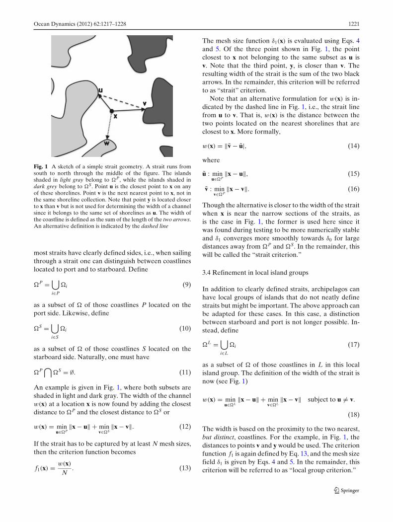
Fig. 1 A sketch of a simple strait geometry. A strait runs fromsouth to north through the middle of the figure. The islandsshaded in light gray belong to �P, while the islands shaded indark grey belong to �S. Point u is the closest point to x on anyof these shorelines. Point v is the next nearest point to x, not inthe same shoreline collection. Note that point y is located closerto x than v but is not used for determining the width of a channelsince it belongs to the same set of shorelines as u. The width ofthe coastline is defined as the sum of the length of the two arrows.An alternative definition is indicated by the dashed line

most straits have clearly defined sides, i.e., when sailingthrough a strait one can distinguish between coastlineslocated to port and to starboard. Define

�P =⋃i∈P

�i (9)

as a subset of � of those coastlines P located on theport side. Likewise, define

�S =⋃i∈S

�i (10)

as a subset of � of those coastlines S located on thestarboard side. Naturally, one must have

�P⋂

�S = ∅. (11)

An example is given in Fig. 1, where both subsets areshaded in light and dark gray. The width of the channelw(x) at a location x is now found by adding the closestdistance to �P and the closest distance to �S or

w(x) = minu∈�P

‖x − u‖ + minv∈�S

‖x − v‖. (12)

If the strait has to be captured by at least N mesh sizes,then the criterion function becomes

f1(x) = w(x)

N. (13)

The mesh size function δ1(x) is evaluated using Eqs. 4and 5. Of the three point shown in Fig. 1, the pointclosest to x not belonging to the same subset as u isv. Note that the third point, y, is closer than v. Theresulting width of the strait is the sum of the two blackarrows. In the remainder, this criterion will be referredto as “strait” criterion.

Note that an alternative formulation for w(x) is in-dicated by the dashed line in Fig. 1, i.e., the strait linefrom u to v. That is, w(x) is the distance between thetwo points located on the nearest shorelines that areclosest to x. More formally,

w(x) = ‖v − u|, (14)

where

u : minu∈�P

‖x − u‖, (15)

v : minv∈�P

‖x − v‖. (16)

Though the alternative is closer to the width of the straitwhen x is near the narrow sections of the straits, asis the case in Fig. 1, the former is used here since itwas found during testing to be more numerically stableand δ1 converges more smoothly towards δ0 for largedistances away from �P and �S. In the remainder, thiswill be called the “strait criterion.”

3.4 Refinement in local island groups

In addition to clearly defined straits, archipelagos canhave local groups of islands that do not neatly definestraits but might be important. The above approach canbe adapted for these cases. In this case, a distinctionbetween starboard and port is not longer possible. In-stead, define

�L =⋃i∈L

�i (17)

as a subset of � of those coastlines in L in this localisland group. The definition of the width of the strait isnow (see Fig. 1)

w(x) = minu∈�L

‖x − u‖ + minv∈�L

‖x − v‖ subject to u = v.

(18)

The width is based on the proximity to the two nearest,but distinct, coastlines. For the example, in Fig. 1, thedistances to points v and y would be used. The criterionfunction f1 is again defined by Eq. 13, and the mesh sizefield δ1 is given by Eqs. 4 and 5. In the remainder, thiscriterion will be referred to as “local group criterion.”

1222 Ocean Dynamics (2012) 62:1217–1228

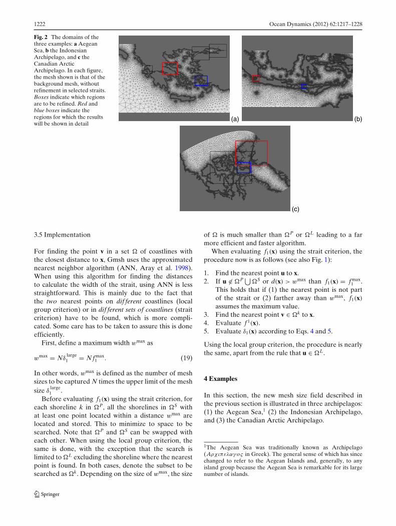
Fig. 2 The domains of thethree examples: a AegeanSea, b the IndonesianArchipelago, and c theCanadian ArcticArchipelago. In each figure,the mesh shown is that of thebackground mesh, withoutrefinement in selected straits.Boxes indicate which regionsare to be refined. Red andblue boxes indicate theregions for which the resultswill be shown in detail

(a) (b)

(c)

3.5 Implementation

For finding the point v in a set � of coastlines withthe closest distance to x, Gmsh uses the approximatednearest neighbor algorithm (ANN, Aray et al. 1998).When using this algorithm for finding the distancesto calculate the width of the strait, using ANN is lessstraightforward. This is mainly due to the fact thatthe two nearest points on dif ferent coastlines (localgroup criterion) or in dif ferent sets of coastlines (straitcriterion) have to be found, which is more compli-cated. Some care has to be taken to assure this is doneefficiently.

First, define a maximum width wmax as

wmax = Nδlarge1 = N f max

1 . (19)

In other words, wmax is defined as the number of meshsizes to be captured N times the upper limit of the meshsize δ

large1 .

Before evaluating f1(x) using the strait criterion, foreach shoreline k in �P, all the shorelines in �S withat least one point located within a distance wmax arelocated and stored. This to minimize to space to besearched. Note that �P and �S can be swapped witheach other. When using the local group criterion, thesame is done, with the exception that the search islimited to �L excluding the shoreline where the nearestpoint is found. In both cases, denote the subset to besearched as �k. Depending on the size of wmax, the size

of � is much smaller than �P or �L leading to a farmore efficient and faster algorithm.

When evaluating f1(x) using the strait criterion, theprocedure now is as follows (see also Fig. 1):

1. Find the nearest point u to x.2. If u ∈ �P ⋃

�S or d(x) > wmax than f1(x) = f max1 .

This holds that if (1) the nearest point is not partof the strait or (2) farther away than wmax, f1(x)

assumes the maximum value.3. Find the nearest point v ∈ �k to x.4. Evaluate f 1(x).5. Evaluate δ1(x) according to Eqs. 4 and 5.

Using the local group criterion, the procedure is nearlythe same, apart from the rule that u ∈ �L.

4 Examples

In this section, the new mesh size field described inthe previous section is illustrated in three archipelagos:(1) the Aegean Sea,1 (2) the Indonesian Archipelago,and (3) the Canadian Arctic Archipelago.

1The Aegean Sea was traditionally known as Archipelago(Aρχιπελαγ oς in Greek). The general sense of which has sincechanged to refer to the Aegean Islands and, generally, to anyisland group because the Aegean Sea is remarkable for its largenumber of islands.

Ocean Dynamics (2012) 62:1217–1228 1223

Table 1 Parameters used for producing the example meshes

Parameter Aegean Indonesian Canadian ArcticSea Archipelago Archipelago

f small0 0.025 0.025 5.0

f large0 25.000 25.000 250.0

δmin0 0.025 0.025 5.0

δmax0 5.000 5.000 50.0

f small1 0.000 0.000 0.0

f large1 25.000 25.000 250.0

δmin1 0.000 0.000 0.0

δmax1 5.000 5.000 50.0

Subscript 0 refers to the criterion function based on the prox-imity to the coastline (see Eq. 8) and subscript 1 refers to therefinement in narrow straits and island groups (see Eq. 13).The parameters refer to those used in Eq. 4 to evaluate thecorresponding mesh size functions

Figure 2 shows the spatial extent of each domain.In addition, the background mesh, without refinement,is shown. This mesh is produced based only on theproximity to the coastline (Eq. 8), using the top four(those with subscript 0) in Table 1. Since this is theunrefined mesh, in the remainder of the text, N = 0for this mesh. Note that depending on the width ofthe strait, the background mesh might have at somelocations only one element across.

The background mesh is further refined by using themesh size field (Eq. 13) above for several values of thedesired resolution N. The parameters used for meshingthe domains are shown in Table 1.

These examples, as well as the areas of refinement,have been chosen to illustrate the mesh size field de-scribed above. We do not intend to make statementsabout whether those resolutions are necessary to re-solve the physical processes that might be important inthose areas.

4.1 Aegean Sea

The domain that covers theAegean Sea and surround-ing areas is shown Fig. 2a. It includes the Bosporus andSea of Marmara, which connects the Aegean Sea withthe Black Sea to the northeast (not shown). Parts of theeastern Mediterranean are also included.

Regions that will be refined are indicated by the box-es in Fig. 2a. The results of the meshing refinement areonly shown for the red and blue boxes: (1) the EuboicGulf between the Greek mainland and the Island ofEuboea (located within the red box) and (2) the IcarianSea (located within the blue box). The results are shownin Figs. 3 and 4, respectively. In these figures, as well asthe next few, each triangular element is colored withrespect to the log10 of the radius of the circumcircle of

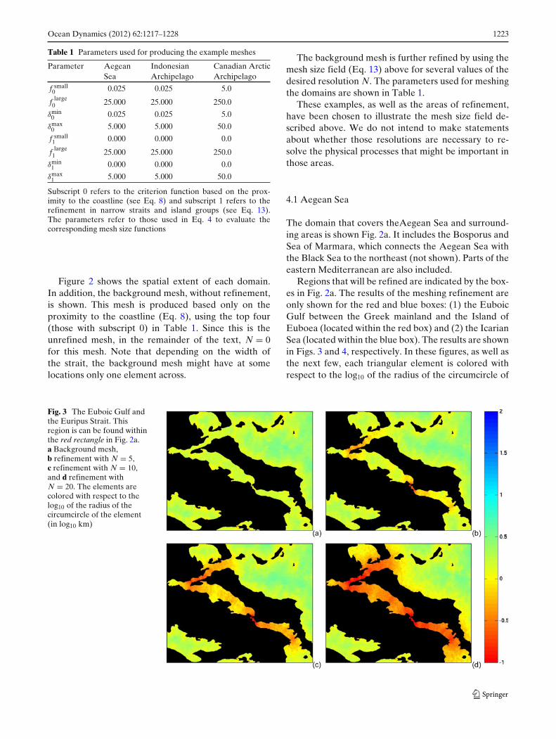
Fig. 3 The Euboic Gulf andthe Euripus Strait. Thisregion is can be found withinthe red rectangle in Fig. 2a.a Background mesh,b refinement with N = 5,c refinement with N = 10,and d refinement withN = 20. The elements arecolored with respect to thelog10 of the radius of thecircumcircle of the element(in log10 km)

1224 Ocean Dynamics (2012) 62:1217–1228

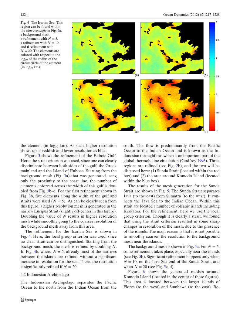
Fig. 4 The Icarian Sea. Thisregion can be found withinthe blue rectangle in Fig. 2a.a background mesh,b refinement with N = 5,c refinement with N = 10,and d refinement withN = 20. The elements arecolored with respect to thelog10 of the radius of thecircumcircle of the element(in log10 km)

the element (in log10 km). As such, higher resolutionshows up as reddish and lower resolution as blue.

Figure 3 shows the refinement of the Euboic Gulf.Here, the strait criterion was used, since one can clearlydiscriminate between both sides of the gulf: the Greekmainland and the Island of Euboea. Starting from thebackground mesh (Fig. 3a) that was generated usingonly the proximity to the coast line, the number ofelements enforced across the width of this gulf is dou-bled from Fig. 3b–d. For the first refinement shown inFig. 3b, five elements along the width of the gulf andstraits were used (N = 5). As can be clearly seen fromthis figure, a higher resolution mesh is generated in thenarrow Euripus Strait (slightly off-center in this figure).Doubling the value of N results in higher resolutionmesh while smoothly going to the coarser resolution ofthe background mesh away from this area.

The refinement for the Icarian Sea is shown inFig. 4. Here, the local group criterion was used, sinceno clear strait can be distinguished. Starting from thebackground mesh, the mesh is refined by doubling N.In Fig. 4b, where N = 5, already most of the narrowsbetween the islands are refined, without a significantincrease in resolution for the sea. There, the resolutionis significantly refined if N = 20.

4.2 Indonesian Archipelago

The Indonesian Archipelago separates the PacificOcean to the north from the Indian Ocean from the

south. The flow is predominantly from the PacificOcean to the Indian Ocean and is known as the In-donesian throughflow, which is an important part of theglobal thermohaline circulation (Godfrey 1996). Threeregions are refined (see Fig. 2b), and the two will bediscussed here: (1) Sunda Strait (located within the redbox) and (2) the area around Komodo Island (locatedwithin the blue box).

The results of the mesh generation for the SundaStrait are shown in Fig. 5. The Sunda Strait separatesJava (to the east) from Sumatra (to the west). It con-nects the Java Sea to the Indian Ocean. Within thisstrait are located a number of volcanic islands includingKrakatoa. For the refinement, here we use the localgroup criterion. Though it is clearly a strait, we foundthat using the strait criterion resulted in some sharpchanges in resolution of the mesh, due to the presenceof the islands. The main reason is that it is not possibleto smoothly coarsen the resolution to the backgroundmesh near the islands.

The background mesh is shown in Fig. 5a. For N = 5,some refinement takes place, especially near the islands(see Fig. 5b). Significant refinement happens only whenN = 10, on the Java Sea end of the Sunda Strait, andwhen N = 20 (see Fig. 5c ,d).

Figure 6 shows the generated meshes aroundKomodo Island (located in the center of these figures).This area is located between the larger islands ofFlores (to the west) and Sumbawa (to the east). Be-

Ocean Dynamics (2012) 62:1217–1228 1225

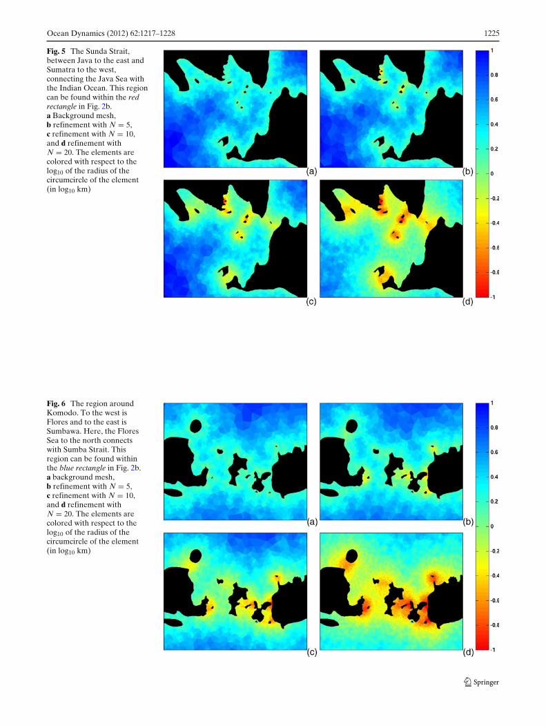
Fig. 5 The Sunda Strait,between Java to the east andSumatra to the west,connecting the Java Sea withthe Indian Ocean. This regioncan be found within the redrectangle in Fig. 2b.a Background mesh,b refinement with N = 5,c refinement with N = 10,and d refinement withN = 20. The elements arecolored with respect to thelog10 of the radius of thecircumcircle of the element(in log10 km)

Fig. 6 The region aroundKomodo. To the west isFlores and to the east isSumbawa. Here, the FloresSea to the north connectswith Sumba Strait. Thisregion can be found withinthe blue rectangle in Fig. 2b.a background mesh,b refinement with N = 5,c refinement with N = 10,and d refinement withN = 20. The elements arecolored with respect to thelog10 of the radius of thecircumcircle of the element(in log10 km)

1226 Ocean Dynamics (2012) 62:1217–1228

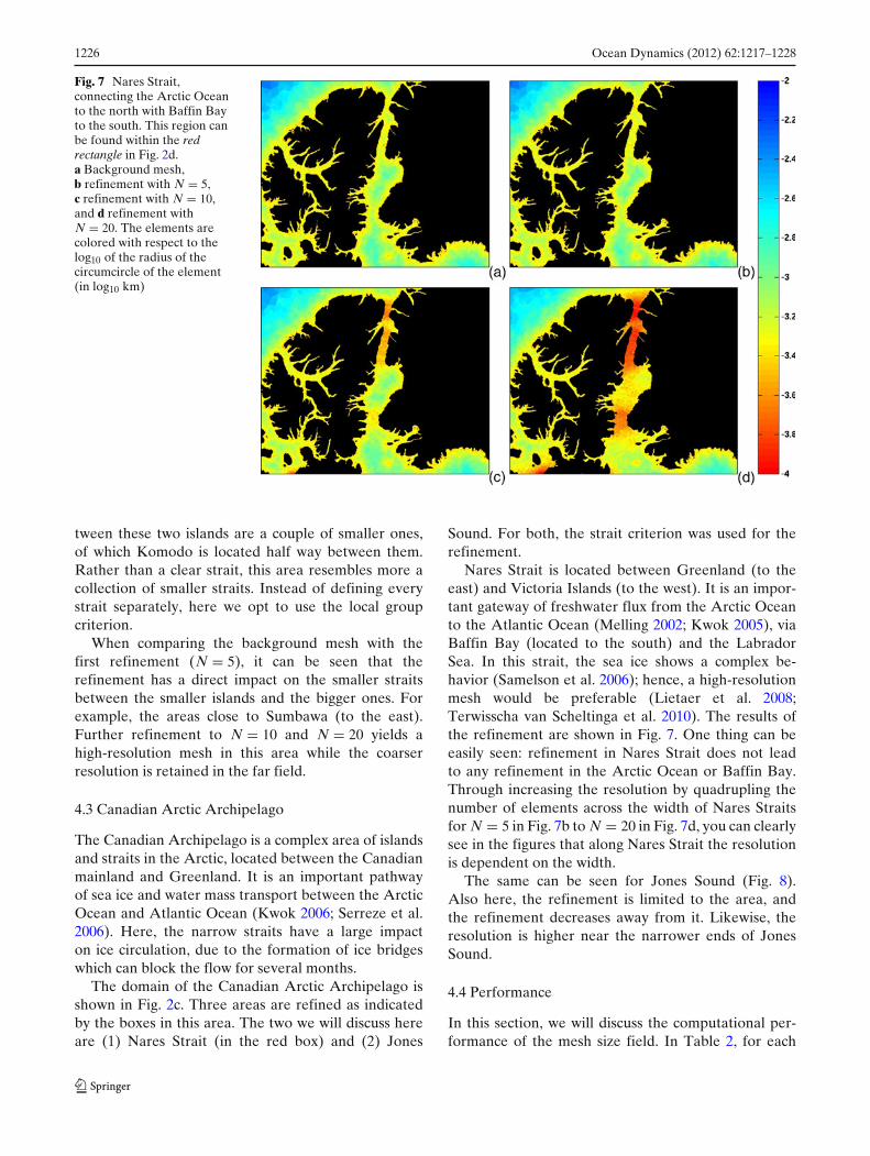
Fig. 7 Nares Strait,connecting the Arctic Oceanto the north with Baffin Bayto the south. This region canbe found within the redrectangle in Fig. 2d.a Background mesh,b refinement with N = 5,c refinement with N = 10,and d refinement withN = 20. The elements arecolored with respect to thelog10 of the radius of thecircumcircle of the element(in log10 km)

tween these two islands are a couple of smaller ones,of which Komodo is located half way between them.Rather than a clear strait, this area resembles more acollection of smaller straits. Instead of defining everystrait separately, here we opt to use the local groupcriterion.

When comparing the background mesh with thefirst refinement (N = 5), it can be seen that therefinement has a direct impact on the smaller straitsbetween the smaller islands and the bigger ones. Forexample, the areas close to Sumbawa (to the east).Further refinement to N = 10 and N = 20 yields ahigh-resolution mesh in this area while the coarserresolution is retained in the far field.

4.3 Canadian Arctic Archipelago

The Canadian Archipelago is a complex area of islandsand straits in the Arctic, located between the Canadianmainland and Greenland. It is an important pathwayof sea ice and water mass transport between the ArcticOcean and Atlantic Ocean (Kwok 2006; Serreze et al.2006). Here, the narrow straits have a large impacton ice circulation, due to the formation of ice bridgeswhich can block the flow for several months.

The domain of the Canadian Arctic Archipelago isshown in Fig. 2c. Three areas are refined as indicatedby the boxes in this area. The two we will discuss hereare (1) Nares Strait (in the red box) and (2) Jones

Sound. For both, the strait criterion was used for therefinement.

Nares Strait is located between Greenland (to theeast) and Victoria Islands (to the west). It is an impor-tant gateway of freshwater flux from the Arctic Oceanto the Atlantic Ocean (Melling 2002; Kwok 2005), viaBaffin Bay (located to the south) and the LabradorSea. In this strait, the sea ice shows a complex be-havior (Samelson et al. 2006); hence, a high-resolutionmesh would be preferable (Lietaer et al. 2008;Terwisscha van Scheltinga et al. 2010). The results ofthe refinement are shown in Fig. 7. One thing can beeasily seen: refinement in Nares Strait does not leadto any refinement in the Arctic Ocean or Baffin Bay.Through increasing the resolution by quadrupling thenumber of elements across the width of Nares Straitsfor N = 5 in Fig. 7b to N = 20 in Fig. 7d, you can clearlysee in the figures that along Nares Strait the resolutionis dependent on the width.

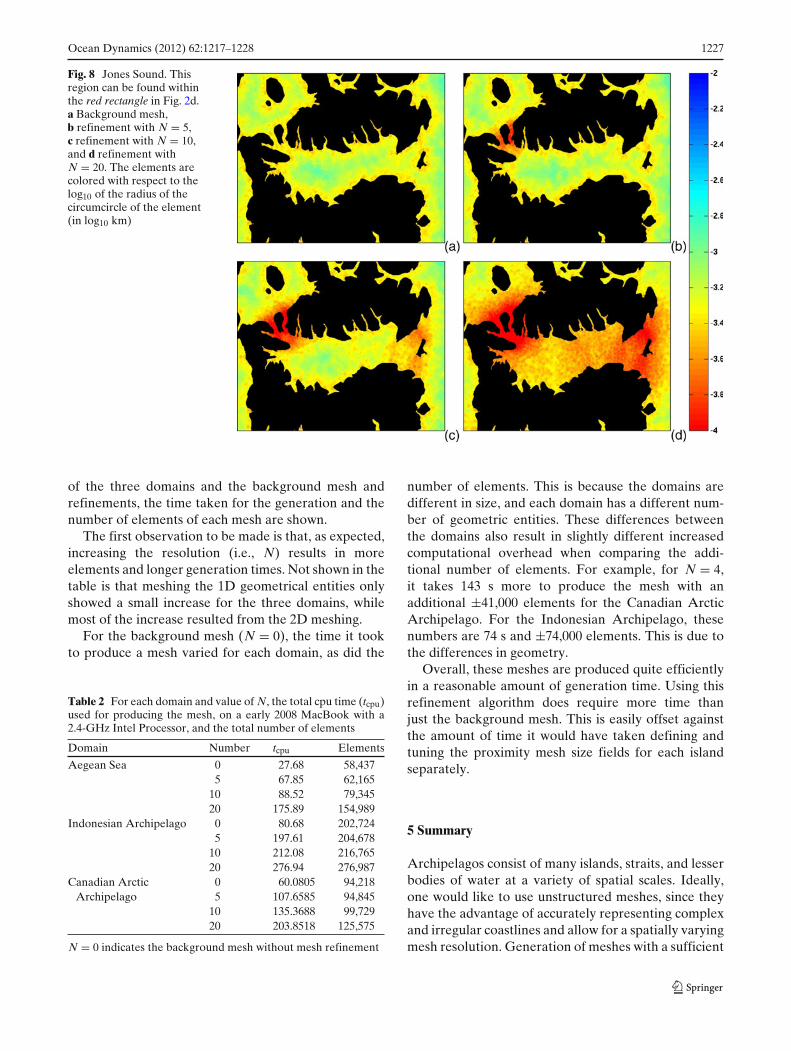
The same can be seen for Jones Sound (Fig. 8).Also here, the refinement is limited to the area, andthe refinement decreases away from it. Likewise, theresolution is higher near the narrower ends of JonesSound.

4.4 Performance

In this section, we will discuss the computational per-formance of the mesh size field. In Table 2, for each

Ocean Dynamics (2012) 62:1217–1228 1227

Fig. 8 Jones Sound. Thisregion can be found withinthe red rectangle in Fig. 2d.a Background mesh,b refinement with N = 5,c refinement with N = 10,and d refinement withN = 20. The elements arecolored with respect to thelog10 of the radius of thecircumcircle of the element(in log10 km)

of the three domains and the background mesh andrefinements, the time taken for the generation and thenumber of elements of each mesh are shown.

The first observation to be made is that, as expected,increasing the resolution (i.e., N) results in moreelements and longer generation times. Not shown in thetable is that meshing the 1D geometrical entities onlyshowed a small increase for the three domains, whilemost of the increase resulted from the 2D meshing.

For the background mesh (N = 0), the time it tookto produce a mesh varied for each domain, as did the

Table 2 For each domain and value of N, the total cpu time (tcpu)used for producing the mesh, on a early 2008 MacBook with a2.4-GHz Intel Processor, and the total number of elements

Domain Number tcpu Elements

Aegean Sea 0 27.68 58,4375 67.85 62,165

10 88.52 79,34520 175.89 154,989

Indonesian Archipelago 0 80.68 202,7245 197.61 204,678

10 212.08 216,76520 276.94 276,987

Canadian Arctic 0 60.0805 94,218Archipelago 5 107.6585 94,845

10 135.3688 99,72920 203.8518 125,575

N = 0 indicates the background mesh without mesh refinement

number of elements. This is because the domains aredifferent in size, and each domain has a different num-ber of geometric entities. These differences betweenthe domains also result in slightly different increasedcomputational overhead when comparing the addi-tional number of elements. For example, for N = 4,it takes 143 s more to produce the mesh with anadditional ±41,000 elements for the Canadian ArcticArchipelago. For the Indonesian Archipelago, thesenumbers are 74 s and ±74,000 elements. This is due tothe differences in geometry.

Overall, these meshes are produced quite efficientlyin a reasonable amount of generation time. Using thisrefinement algorithm does require more time thanjust the background mesh. This is easily offset againstthe amount of time it would have taken defining andtuning the proximity mesh size fields for each islandseparately.

5 Summary

Archipelagos consist of many islands, straits, and lesserbodies of water at a variety of spatial scales. Ideally,one would like to use unstructured meshes, since theyhave the advantage of accurately representing complexand irregular coastlines and allow for a spatially varyingmesh resolution. Generation of meshes with a sufficient

1228 Ocean Dynamics (2012) 62:1217–1228

resolution in archipelagos is not a straightforward task.To produce a mesh, see Lambrechts et al. (2008) for aprocedure on how one would need to define a mesh sizefield that defines the resolution at every spatial point. Apopular choice of such a field is based on the proximityto the nearest coastline. For archipelagos, one wouldhave to define and tune for every coastline such a meshsize field in order to get the required resolution in therelevant straits of the archipelago. This is an inefficientand labor-intensive approach.

Here, we have introduced an extension of the meshsize field that is based on the proximity. We use theproximity to the two nearest coastlines to determine thewidth of a strait or separation between two islands. Thisis then used to determine the mesh size field by dividingthis length by the number of required elements. Thisnew mesh size field is illustrated for three examples ofarchipelagos: (1) the Aegean Sea, (2) the IndonesionArchipelago, and (3) the Canadian Arctic Archipelago.

Acknowledgement This study received funding support fromArcticnet.

References

Adcroft A, Marshall D (1998) How slippery are piecewise-constant coastlines in numerical ocean models? Tellus50A:95–108

Aray S, Mount D, Netanyahu N, Silverman R, Wu A (1998) Anoptimal algorithm for approximate nearest neighbor search-ing. J ACM 45:891–923

Danilov S, Kivman G, Schröter J (2005) Evaluation of aneddy-permitting finite element model in the North Atlantic.Ocean Model 10:35–49

George PL, Frey P (2000) Mesh generation. Hermes, LyonGeuzaine C, Remacle JF (2009) Gmsh: a three-dimensional

finite element mesh generator with built-in pre- and post-processing facilities. Int J Numer Methods Eng 79:1309–1331

Godfrey J (1996) The effect of the Indonesian throughflow onocean circulation and heat exchange with the atmosphere: areview. J Geophys Res 101:C12,217

Gorman G, Piggott M, Pain C, de Oliveira C, Umpleby A,Goddard A (2006) Optimization based bathymetry approx-imation through constrained unstructured mesh adaptivity.Ocean Model 12:436–452

Gorman G, Piggott M, Pain C (2007) Shoreline approximationfor unstructured mesh generation. Comput Geosci 33:666–667

Griffies S, Böning F, Chassignet E, Gerdes R, Hasumi H, Hisrt A,Treguier AM, Webb D (2000) Developments in ocean cli-mate modeling. Ocean Model 2:123–192

Hagen S, Westerink J, Kolar R, Horstmann O (2001) Two-dimensional, unstructured mesh generation for tidal models.Int J Numer Methods Fluids 35:669–686

Henry R, Waters R (1993) Geometrically based, automatic gen-erator for irregular triangular networks. Commun NumerMethods Eng 9:555–566

Kwok R (2005) Variability of Nares Strait ice flux. Geophys ResLett 32:L24,502

Kwok R (2006) Exchange of sea ice between the Arctic Oceanand the Canadian Arctic Arcipelago. Geophys Res Lett33:L16,501

Lambrechts J, Comblen R, Legat V, Geuzaine C, Remacle JF(2008) Multiscale mesh generation on the sphere. OceanDyn 58:461–473

Le Provost C, Genco ML, F Lyard, Vinvent P, Canceil P (1994)Spectroscopy of the world ocean tides from a finite elementhydrodynamic model. J Geophys Res 99:777–797

Lee T, Fukumori I, Menemenlis D, Xing Z, Fu LL (2002) Effectsof the Indonesian throughflow on the Pacific and IndianOceans. J Phys Ocean 32:1404–1429

Legrand S, Legat V, Deleersnijder E (2000) Delaunay mesh gen-eration for an unstructured-grid ocean circulation model.Ocean Model 2:17–28

Legrand S, Deleersnijder E, Hanert E, Legat V, Wolaski E(2006) High-resolution, unstructured meshes for hydrody-namic models of the Great Barrier Reef, Australia. EstuarCoast Shelf Sci 68:36–46

Li X, Shephard M, Beall M (2005) 3d anisotropic mesh adap-tation by mesh modification. Comput Methods Appl MechEng 194:4915–4950

Lietaer O, Fichefet T, Legat V (2008) The effects of resolvingthe Canadian Arctic Archipelago in a finite element sea icemodel. Ocean Model 24:114–152

Lyard F, Lefevre F, Letellier T, Francis O (1994) Modelling theglobal ocean tides: modern insights from fes2004. OceanDyn 56:394–415

Melling H (2002) Sea ice cover in the northern Canadian ArcticArchipelago. J Geophys Res 107:3181

Pain C, Piggott M, Goddard A, Fang F, Gorman G, Marshall D,Eaton M, Power P, de Oliveira C (2005) Three-dimensionalunstructured mesh ocean modelling. Ocean Model 10:5–33

Piggott M, Gorman G, Pain C (2007) Multi-scale ocean modellingwith adaptive unstructured grids. CLIVAR Exch OceanModel Dev Assess 12:21–23

Rebay S (1993) Efficient unstructured mesh generation by meansof delaunay triangulation and Bowyer–Watson algorithm.Comput Phys 106:25–138

Samelson R, Agnew T, Melling H, Munchow A (2006) Evidencefor atmospheric control of sea-ice motion through naresstrait. Geo Rev Let 33:L02,506

Schneider N (1998) The Indonesian throughflow and the globalclimate system. J Climate 11:676–689

Serreze M, Barrett A, Slater A, Woodgate RA, Aagaard K, Lam-mers R, Steele M, Moritz R, Meredith M, Lee C (2006) Thelarge-scale freshwater cycle of the Arctic. J Geophys Res111:C11,010

Terwisscha van Scheltinga A, Myers P, Pietrzak J (2010) A finiteelement sea ice model of the Canadian Arctic Archipelago.Ocean Dyn 60:1539–1558

Wessel P, Smith W (1996) A global, self-consistent, hierar-chical, high-resolution shoreline database. J Geophys Res101:8741–8743

White L, Deleersnijder E, Legat V (2008) A three-dimensionalunstructured mesh finite element method shallow-watermodel, with application to the flows around an island andin a wind-driven, elongated basin. Ocean Model 22:26–47