melissa ann kershner
TRANSCRIPT
Thermoforming Plastic Cups and Cones
by
MELISSA ANN KERSHNER
A thesis submitted in partial fulfillment of the requirement for the degree of
MASTER OF SCIENCE
in Mechanical Engineering
at the
UNIVERSITY OF WISCONSIN-MADISON
2007

Approved
___________________________________
A. Jeffrey Giacomin
Professor of Mechanical Engineering
Date____________
iii
Table of Contents
Part I: Thermoforming Cones
Abstract
I. Introduction
II. Thermoforming Mechanics
III. Free Forming Geometry
IV. Free Forming Results
V. Constrained Forming Geometry
VI. Constrained Forming Results
VII. Plug Assist
VIII. Worked Examples
A. Process speed and melt stress
B. Pressure difference and part height
C. Cone sharpness
D. Plug assist
IX. Conclusion
X. Acknowledgement
Appendix : Thin Film Approximation
Part II: Thermoforming Cups
Abstract
I. Introduction
II. Finite Element Procedures
1
1
7
10
11
14
17
19
22
22
24
24
25
26
26
27
28
29
31

iv
A. Cup Specifications
B. Plug Assisted Model
C. Viscoelastic Models
1. Nonlinear Function
2. Linear Function
D. Material Characterization
1. Discrete Relaxation Spectrum
2. Single Relaxation Time Calculation
E. Plug Heat Transfer
F. Simulation Variation
III. Experimental Procedures
A. Plant and Laboratory Data
B. Method for Comparison of Simulation and Data
IV. Results
V. Discussion
VI. Conclusion
VII. Acknowledgement
References
32
33
36
37
39
39
39
40
41
41
42
42
43
43
50
52
52
53

v
ACKNOWLEDGEMENT
I am deeply grateful to my advisor Professor Giacomin, whose knowledge and insight I
could not have finished without. I would especially like to thank him and the other
committee members Professor Osswald and Professor Turng for their support and
guidance. Also, through their courses I have gained valuable knowledge that I will use
for the rest of my career.
Thank you to Dr. Jaydeep Kulkarni of Fluent Corporation for guidance with the Finite
Element software. I am also indebted to the Fluent Corporation for generously extending
an academic license to the Rheology Research Center of the University of Wisconsin for
the POLYFLOW finite element simulation software.
Also, I am grateful to Dr. Zhongbao Chen of the University of Wisconsin and Dr. Martin
Stephenson for their technical advice. I also wish to acknowledge Professor R. Byron
Bird of the University of Wisconsin for his help with the thin film approximation.
I would also like to extend a special thanks to the students of the Polymer Engineering
Society and in my lab. They have given me very helpful direction during my research. I
have thoroughly enjoyed working with them.
Last but not least, thank you to all the members of the Industrial Consortium of the
Center for Advanced Polymer for financial support, especially the Placon Corporation of
Madison, Wisconsin and Plastics Ingenuity Inc. of Cross Plains, Wisconsin.

vi
DEDICATION
To my family and future husband Andrew Ju for all their love and support.

vii
List of Figures
Part I: Thermoforming Cones
Figure 1 : Thin sphere transitioning
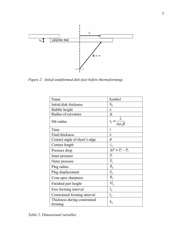
Figure 2: Initial undeformed disk (just before thermoforming).
Figure 5: Dimensional schematic of transitioning cone
Figure 3: Dimensionless radius of curvature as a function of dimensionlesstime
Figure 4: Dimensionless stress versus dimensionless radius of curvature
Figure 6: Plug assist
Part II: Thermoforming Cups
Figure 7: Cup with labeled axis
Figure 8: Simulated Cup
Figure 9: Initial position of polymer sheet, plug and mold before any contactoccurs
Figure 10: Plug stretching the polymer sheet. The sheet has not yet touchedthe mold
Figure 11: Screenshot taken as the sheet is inflated. It is no longer touchingthe plug and just beginning to touch the mold at the top. The total plugcontact time is 1.02 s.
Figure 12: Final sheet position just after the after it freezes into position inthe mold. The total mold contact time is 0.02 s.
Figure 13: Simulation comparison with data for discrete spectrum and singlerelaxation time fluid.
Figure 14: Effect of plug temperature.
Figure 15: Effect of draw depth ratio
4
5
12
14
16
20
32
33
34
35
35
36
44
46
47

viii
Figure 17: Simulation results from the values for nonlinear viscoelastic
Figure 16: Effect of for viscoelastic cases: nonlinear versus linear
48
49

1
Part I: Thermoforming Cones Abstract This new analysis for thermoforming cones focuses on the manufacturing process speed.
Specifically, this work distinguishes between what happens before and after (free versus
constrained forming) the melt touches the conical mold. Analytical solutions are derived
for the time required for both cases, and sum them to get the total forming time. This
analysis is restricted to the Newtonian fabrication of cones, the simplest relevant problem
in commercial thermoforming.
I. Introduction Thermoforming is the mass production of thin non-hollow products from uniformly thick
flat sheets. We divide modern commercial thermoforming into four phases. Firstly, in
free forming (φ ), a thin untouched sheet deforms under an applied air pressure. In plug
assisted forming (π ), a carefully designed solid shape then touches and stretches some
of the sheet to reshape it. The parts touching the plug do not stretch. Once released from
this plug, the reshaped sheet again deforms freely till it contacts the mold. The material
not yet touching the mold then continues to stretch till the mold is covered and we call
this constrained forming (κ ). Sometimes, thermoforming is done without the plug
assist and this paper attacks this special case. Tadmor and Gogos [1] call this straight
thermoforming. We solve for both the mold covering speed and the product thickness
profile. Table 1 compares this paper with previous work.

2
We begin by modeling free forming, where a uniformly thin polymeric film is formed
from a thin flat disk inflated through a round hole into a growing thin sphere. Williams
[4] confirmed this spherical shape experimentally. These thin spheres transition from
lenticular, through hemispherical, to bulbous as illustrated in Figure 1. Figure 2
illustrates the initial condition, a flat disk of thickness 0h , and thus of infinite radius of
curvature, R .
We restrict this analysis to Newtonian liquids, so we expect this work will apply
accurately to low molecular weight systems such as polyester which is commonly used to
thermoform stiff clear packaging. Our analytical solutions also provide benchmarks for
numerical analysts to test their code accuracy. We further restrict our analysis to the
fabrication of cones, the simplest product shape in commercial thermoforming.
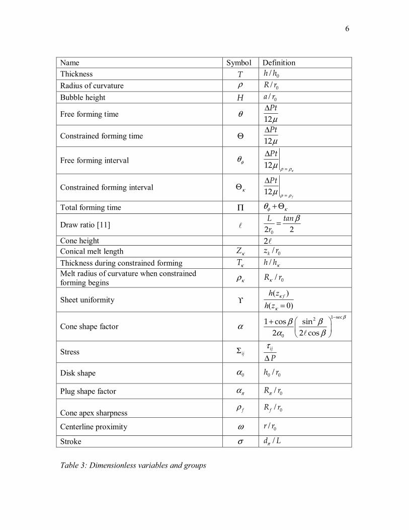
Table 2 summarizes these and other dimensional variables. Furthermore, Table 3 defines
the corresponding dimensionless variables, including thickness (T), radius of curvature
( ρ ) and height (H ) of the free forming bubble.

3
Cyl
inde
r
Con
e
Trun
cate
d C
one
Wed
ge
Trun
cate
d W
edge
Phas
es
Tens
ile S
tress
es
Geo
met
ry
Con
stitu
tive
Beh
avio
r
Uni
form
Thi
ckne
ss
Spee
d
Ref
eren
ce
Hart-Smith and Crisp (1967)
φ X X σ [2]
Sheryshev et al. (1969) X κ X X [3]
Williams (1970) X X ,φ π X X σ X [4]
Williams (1970) X X ,κ π X X σ [4]
Tadmor and Gogos (1979)
X κ X X [1]
Rosenzweig et al. (1979) X X κ X X [5]
Throne (1979) X ,κ π X σ X [6]
Pearson (1985) X X X κ X X σ X [7]
Allard et al. (1986) X X ,φ κ X X λ X [8]
Baird and Collias (1998)
X κ X λ X [9]
Osswald and Hernández –Ortiz (2006)
X κ X X [10]
This Paper X X , ,φ π κ X X λ X X
Table 1: Previous work [free forming (φ ), plug assisted forming (π ), constrained forming (κ ); liquid ( λ ), solid (σ )]

4
Figure 1 : Thin sphere transitioning
5
Figure 2: Initial undeformed disk (just before thermoforming).
Name Symbol Initial disk thickness 0h Bubble height a Radius of curvature R
Slit radius β≡0
Lrtan
Time t Final thickness h Contact angle of sheet’s edge φ Contact length kz Pressure drop ∆ ≡ −i oP P P Inner pressure iP Outer pressure oP Plug radius πR Plug displacement πd
Cone apex sharpness fR
Finished part height pH
Free forming interval φt
Constrained forming interval κt Thickness during constrained forming κh
Table 2: Dimensional variables
6
Name Symbol Definition Thickness T 0h / h Radius of curvature ρ 0R/ r Bubble height H 0a / r
Free forming time θ µ∆12Pt
Constrained forming time Θ µ∆12Pt
Free forming interval φθ κρ ρµ =
∆12Pt
Constrained forming interval κΘ ρ ρµ =
∆12
f
Pt
Total forming time Π φ κθ + Θ
Draw ratio [11] l β=
02 2L tanr
Cone height l2 Conical melt length κZ 0kz / r Thickness during constrained forming κT h / hκ Melt radius of curvature when constrained forming begins κρ 0R / rκ
Sheet uniformity ϒ ( )
( 0)fh z
h zκ
κ =
Cone shape factor α ββ β
α β
− + l
1 sec2
0
1 cos sin2 2 cos
Stress Σ ij τ∆ij
P
Disk shape α0 0 0h / r
Plug shape factor πα 0R / rπ Cone apex sharpness
ρ f 0fR / r
Centerline proximity ω 0r / r
Stroke σ d / Lπ Table 3: Dimensionless variables and groups

7
II. Thermoforming Mechanics For the mechanics of the stretching sheet, we follow the thin membrane approach for
bubble inflation of Baird and Collias [9]. We employ moving spherical coordinates
centered in the bubble. Figure 1 defines r. Assuming constant density, the continuity
equation becomes
( )2 0rr vr
∂ =∂
(1)
Integrating gives:
= 2( )
rA tvr
(2)
where ( )A t is a function of time. On the inside surface (at r R= ) the fluid velocity is
= − &( )rv R R (3) for a lenticular film, and for a bulbous one:
= &( )rv R R (4) hence
= & 2( )A t R R (5) and from continuity
=& 2
2r
R Rv
r (6)
Neglecting fluid inertia, the r-component of the equation of motion reduces to
( )22
10 θθ φφτ ττ
+−∂ ∂= − +∂ ∂ rrp rr r r r
(7)
8
where ijτ is the component of the extra stress tensor corresponding to the flux of jx
momentum in the positive ix direction. Hence, φφτ and θθτ are negative in tension.
Rewriting (7):
2θθ φφτ τ τπ + −∂ =∂
rrrr
r r (8)
where the rr component of the total and extra stress tensors are related by π τ= +rr rr p (9) where at the inside surface π = −rr (R) P(R) (10) and outside, π + = − +rr (R h) P(R h) (11) Integrating, the equation of motion [(7)] gives
θθ φφτ τ τ+ + − ∆ = ∫2R h rr
RP dr
r (12)
For thin films, that is, when:
<<0
1hh
(13)
Bird et al. [12] proposed that the argument for the integral in (12), ( )θθ φφτ τ τ+ − 2 /rr r
will be nearly constant. This is because, for a thin film, neither the stresses
( )θθ φφτ τ τ+ − 2 rr , nor the radial position r , will vary much through the film thickness.
Thus, (12) becomes:
( )θθ φφτ τ τ∆ = + − 2 rrhPR
(14)

9
We call this the thin film approximation, and Appendix A further explores its importance.
We can thus further simplify (14), by specifically evaluating the stresses at r R= :
( )θθ φφτ τ τ∆ = + − 2 rr R
hPR
(15)
For a Newtonian fluid:
θθ φφ
µτ τ µ
−= = − =
&2
3
22 r
R Rvr r
(16)
and
2
3
42
µτ µ ∂= − =
∂
&r
rr
R Rvr r
(17)
Thus the tensile stress inside the stretching film:
3
22
2 R
RRirri
&µττ θθ
−=
−= (18)
exceeds the stress outside:
( )3
22
2 hR
RRorro
+
−=−=
&µττ θθ (19)
by the factor:
3
1
+==
Rh
irr
orr
i
o
ττ
ττ
θθ
θθ (20)
Eliminating the stresses in (15) gives
µ∆ =
&
2
12 R hP
R (21)
which reduces to
ρ ρµ α
∆ =2
012P dT dt
(22)
which has been adimensionalized using Table 3. Hence,

10
ρ ρθ α
=2
0
dd T
(23)
which describes how a thin disk’s shape evolves during thermoforming.1 III. Free Forming Geometry The lenticular spherical cap thickness depends on its radius of curvature as
21;
2
12
≥−+
= TTρ
ρρ (24)
so that
2
1 122 1
dT ;Tdρ ρ ρ
= >−
(25)
and for the bulbous spherical cap
21;
2
12
≤−−
= TTρ
ρρ (26)
so that
2
1 122 1
dT ;Tdρ ρ ρ
−= <−
(27)
The following discontinuity thus occurs
12
14ρ ±→
= ±T
dTd
(28)
We obtain the contact angle of the sheet’s edge (defined in Figure 1) from the bubble’s
slope evaluated at 0r :
1 By definition, the dimensionless radius of curvature, ρ , never falls below unity.
11
0 2
12 1
x r a tanπφρ
=
−= +−
(29)
With difficulty, practitioners can sometimes observe the free forming bubble and measure
its height (defined as a in Figure 1). The dimensionless bubble height depends on its
radius of curvature for the lenticular shape as
2 1 ; 1H Hρ ρ= − − ≥ (30)
and for the bulbous shape
ρ ρ= + − ≤2 1 1H ;H (31)
IV. Free Forming Results Substituting (22) into (21) for T , for a lenticular cap we get
( )ρ ρθ α ρ ρ
=+ −
3
20
2
1
dd
(32)
Integrating gives
α ρθρ ρ ρ
−= − − +
20
41 1 2
4arcsin (33)
for bulbous cap growth, and for lenticular cap growth, we substitute (24) into (21)for T ,
and integrate
( )ρ ρθ α ρ ρ
=− −
3
20
2
1
dd
(34)
to get

12
α ρθ πρ ρ ρ
−= + − − +
20
41 1 2 4
4arcsin (35)
Eqs. (33) and (35) are universal, and central to this paper. From these we see that the
shape switch from lenticular to bulbous always occurs at the same dimensionless time
when,
( )ραθ π= > −0
1 48
(36)
where.
1
0dd ρ
ρθ =
= (37)
Figure 3 illustrates this shape switch.
Figure 3: Dimensionless radius of curvature as a function of dimensionless time.
13
Adimensionalizing (18) gives the dimensionless hoop stress inside the stretching film:
16
ddφφ
ρρ θ
−Σ = (38)
For the lenticular melt,
( )2
023 1
φφρα
ρ ρ
−Σ =+ −
(39)
which is negative and peaks at
32=ρ (40)
where
04 3 0 25727φφα −Σ = ≅ − . (41)
and for the bulbous melt
( )2
023 1
φφρα
ρ ρ
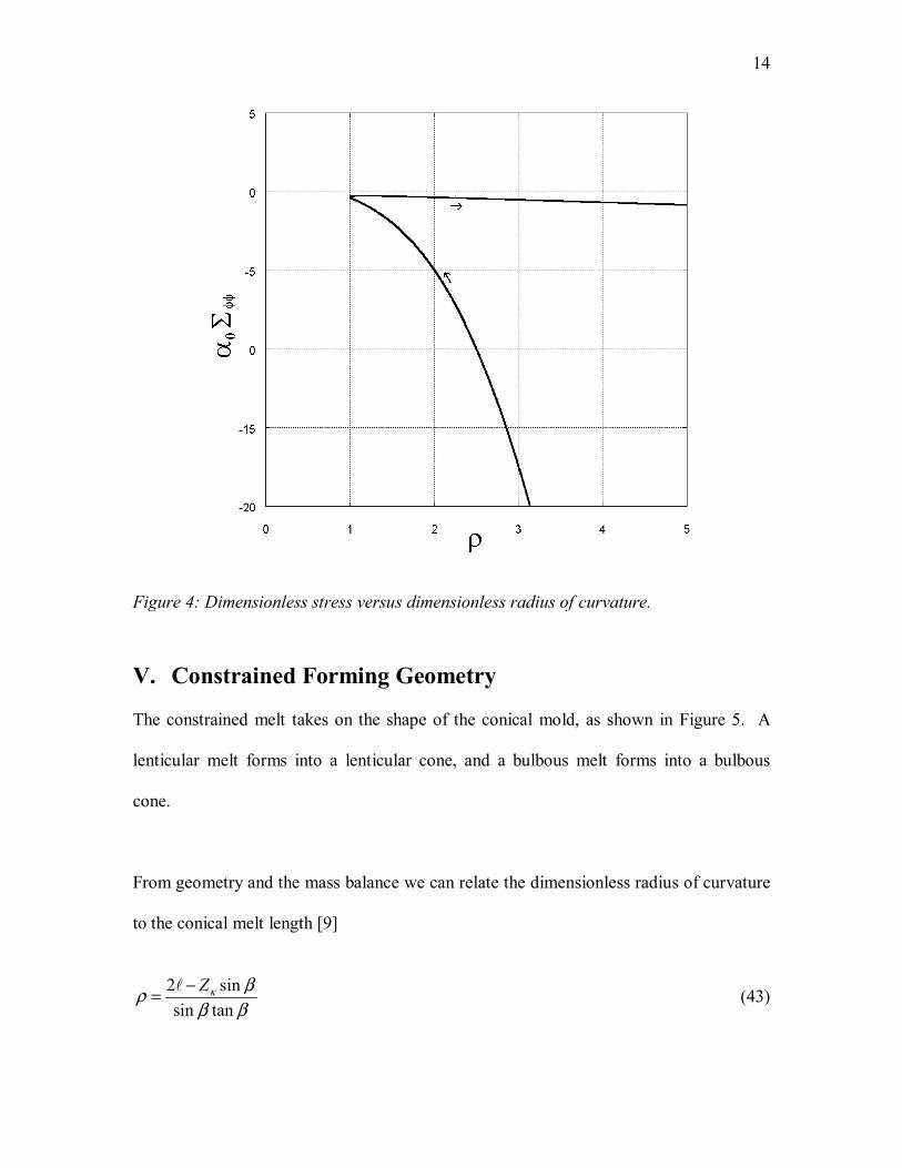
−Σ =− −
(42)
Figure 4 illustrates this. So both the radius of curvature and the magnitude of the tensile
stress, φφΣ , are initially infinite. In practice, there is always a little sag [13, 14], so the
initial radius of curvature is always finite. Furthermore, unlike a rubber, φφΣ is initially
increasing.
14
Figure 4: Dimensionless stress versus dimensionless radius of curvature.
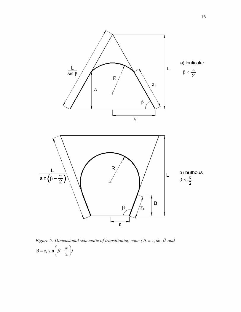
V. Constrained Forming Geometry The constrained melt takes on the shape of the conical mold, as shown in Figure 5. A
lenticular melt forms into a lenticular cone, and a bulbous melt forms into a bulbous
cone.
From geometry and the mass balance we can relate the dimensionless radius of curvature
to the conical melt length [9]
2 sinsin tan
κ βρβ β
−= l Z (43)
15
Now free-forming ends when melt first touches the cone, that is, when 0kZ = . Hence,
2sin tanκρ
β β= l (44)
Substituting into (33) and (35) gives the free-forming intervals, φθ , for the bulbous melt:
κφ
κ κ κ
ραθρ ρ ρ
− = − − +
20
4
11 24
arcsin (45)
and for the lenticular melt:
κφ
κ κ κ
ραθ πρ ρ ρ
− = + − − +
20
4
11 2 44arcsin (46)
respectively. We can also relate the constrained melt thickness t , to the contact length
[1]
βκ
κ β−
= − l
1
12
secZT T sin (47)
From geometry, we can relate the thickness during constrained forming, κh to the initial
disk thickness
2 20
21
4 2L h L ( cos )h
sinκπ π β
β−= (48)
which adimensionalizes to
( )κ β= +0 12TT cos (49)
or
( )κ β= +1 12
T cos (50)
.
16
Figure 5: Dimensional schematic of transitioning cone ( sinA kz β≡ and
sin2
B kz πβ ≡ −
)

17
To get the thickness profile, we substitute (50) into (47):
since 0 1T ≡
( )sec 11 1 cos 1 sin
2 2ZT
βκβ β
− = + − l
(51)
combining (43) and (51)
( )sec 121 sin1 cos
2 2 cosT
ββββ
−
= + l
(52)
When β exceeds 2π , the constrained melt’s shape changes from lenticular to bulbous [1,
4,5,9]. VI. Constrained Forming Results Substituting (52) into (23)
βρ αρθ
−= 3 secdd
(53)
where the cone shape factor is
ββ βαα β
− +≡ l
1 sec2
0
1 cos sin2 2 cos
(54)
where Table 3 defines the dimensionless cone height, l2 (Figure 5 defines the cone
height, L ). When 2πβ < , a lenticular cap progresses down the cone. Hence,
βρ παρ β−= <Θ
3
2secd ;
d (55)
Integrating gives
( )βρ π πβ
α β
−
Θ = > ≠−
2
2 2 3
sec
;sec (56)
18
and
ρ πβα
Θ =log( )=
3; (57)
For thermoforming with 2πβ > , a bulbous cap progresses down the cone. Hence,
βρ παρ β−= − >
Θ3
2secd ;
d (58)
and integrating gives
( )βρ π πβ
α β
−−Θ = > ≠−
sec 2 42 2 3;
sec (59)
and
log( ) 4= 3
ρ πβα
−Θ =; (60)
Linearizing (56) gives
( )( )( )α β πρ β
β β−
= Θ + ≠ − −
212 2 3
ln secln ln ;
sec sec (61)
and linearizing (59):
( )( )( )α β πρ β
β β−
= Θ + ≠ − −
21 4sec 2 sec 2 3
ln secln ln ; (62)
Hence, zero radius of curvature takes an infinite period of constrained forming. In other
words, the melt will never reach the cone apex, and Zκ never reaches 1. Thus, Eqn. (61)
and (62) explain why sharp corners are difficult to thermoform. The thermoforming of
sharp edges or corners is called detailing.
Letting fρ be the desired dimensionless apex sharpness, we then get:

19
( ) ( )κρ ρΘ = Θ − Θf f (63)
for the required constrained forming interval. Thus, the total manufacturing time is
( ) ( )φ
φ κ
θ θ
θ ρ ρ
= + Θ
= + Θ − ΘT f
f (64)
For the melt, the stress is
1 sec
;6 2
β
φφαρ πβ
−−Σ = < (65)
which linearizes to
( ) 1ln 1 sec ln ln6
φφ β ρα
Σ − = − +
(66)
and
1 sec
;6 2
β
φφαρ πβ
−
Σ = > (67)
which linearizes to
( ) 1ln 1 sec ln ln6
φφ β ρα
Σ = − +
(68)
VII. Plug Assist
In thermoforming, plug assist is often used to even out wall thickness profiles. Figure 6
illustrates the variables for plug-assisted thermoforming.

20
Figure 6: Plug assist
Our work focused on unassisted thermoforming, and thus derives the worst case for wall
thickness variation. We define the final wall thickness uniformity as:
( ) ( )
( 0) ( 0)κ κ
κ κ
ϒ ≡ == =
f fh z T Zh z T Z
(69)
where fzκ is the final contact length, corresponding to the final desired radius at the cone tip:
βρβκ tan
sin2
ffZ −= l (70)
Combining (51) with (69) gives:
1
12
secfZ sin β
κ β −
ϒ ≡ − l
(71)
and substituting (70) into this yields:
1
2
secf sin tan βρ β β −
ϒ ≡
l (72)
and in the limit, for an infinitely sharp cone tip, we get:

21
1112
sec
sinβ
β−
ϒ ≡ − l
(73)
which is the worst case for the cone thickness uniformity. Equations (71) and (72)
dictate just how much plug assist is required to even out the cone wall thickness
distribution. Equation (73) gives the upper bound for this plug assist requirement.
From the geometry of the deformation, and in cylindrical coordinates, Williams derived
the following for the thickness profile caused by plug assist
2
0
1
1π
π
≡ +
Tdrr lnR
(74)
and verified this experimentally. This adimensionalizes to
2
121 1
π
ωσ α
≡ + l
T
ln
(75)
where σ is the dimensionless plug displacement (normally called stroke), πα is the plug
shape factor and ω is the center line proximity. So during plug assist, the deforming
melt’s thinnest part is near the plug’s edge where:
2
121 1π
π
ασ α
= + l
minT
ln
(76)
and its thickest, near the mold rim, where:
22
2
121 1 1
πσ α
= + l
maxT
ln
(77)
In principle, we would like to match the severity of the cone thickness problem, ϒ , with
the amount of plug assistance near the rim, maxT . In practice, however, the plug normally
runs into the cone before this amount of plug assistance can be realized. To prevent this,
the stroke must satisfy this geometric inequality:
( )0
0
11
2πα βασα
− < −
l
tan (78)
For a right cylinder, where 2πβ = , the plug can never run into the mold; Throne has
outlined an approach for this special case [6].
VIII. Worked Examples A. Process speed and melt stress A plastics engineer wants to manufacture a safety cone with β = °75 5. and = 31cmL
from a disk of uniform thickness =0 1 51 mmh . and from a nearly Newtonian melt with
µ = × ⋅63 11 10 Pa s. . She desires a blunt cone of apex radius, = 25 4 mmfR . . She
employs an external gage pressure of 91 3 psi. and a vacuum of 14 1 psi. . Calculate the
total forming time, and estimate the stress frozen into the safety cone, both near its rim
and into its blunt tip.
23
Using Table 3, we calculate ( )β≡ =l 2 1 93tan / . . Substituting into (44) gives a
dimensionless radius of curvature of 1.03κρ = when constrained forming begins.
Substituting this and 0 0 0/ 0.0188α ≡ =h r (from Table 3) into (45) then gives a
dimensionless free forming time of 31 85 10φθ −= ×. . Combining ρ ≡ 0R / r from Table 3
with β≡0r L / tan from Table 3 gives the dimensionless radius of curvature of the blunt
cone tip 0 0 312ρ ≡ =f fR / r . . Substituting φθ , κρ , 0 0 312ρ ≡ =f fR / r . and
( ) βα β α β β β
−≡ − =l
1 sec2 20(sin / 2 (1 cos )) sin / 2 cos 36.4 into (64) gives a total
dimensionless forming time of 0 015θ =T . .
Summing the vacuum and the applied air pressures gives ∆ = 105 4 psiP . . Using this and
Table 3, we find the total-forming time of 12 0.770 sµ= Θ ∆ =T Tt / P . We then
substitute κρ , and α = 36.4 , into (65) to obtain the dimensionless stress near the rim of
6.65rimφφΣ = − , which is tensile. We expect most of this to freeze into the rim. Using
Table 3, we find that this corresponds to a tensile stress at the rim of
5.53 MParim rim
Pφφ φφτΣ ∆ = = − , which is also tensile.
Substituting fρ , and α into (65) gives the dimensionless stress near the blunt tip of
253.7tipφφΣ = − , which is tensile. We expect most of this to freeze into the tip. Using
Table 3 we find that this corresponds to a tensile stress at the rim of
211 MPatip tip
Pφφ φφτΣ ∆ = = − .

24
B. Pressure difference and part height
A plastics engineer wants to process the same safety cone as in Example A, but his
process economics require a forming time to fall below 1.2 seconds. Find the required
∆P , finished part height, and estimate the stress frozen into the safety cone, both near its
rim and into its blunt tip.
Using 0 015θ =T . from Example A, for the required applied pressure difference we find
µ∆ = Θ =12 67 7 psiTP / t . . From the cone geometry, for the finished part height we get:
β ββ β
= − − +
f
p f f
RLH sin R tan Rsin tan
(79)
which gives 0.24 m. C. Cone sharpness A plastics engineer wants to manufacture a pointy cone ( )1ρ f with β = °75 5. and
= 0 31mL . from a disk of nearly Newtonian melt with µ = × ⋅63 11 10 Pa s. and uniform
thickness =0 1 51 mmh . . She employs an external gage pressure of 91 3 psi. and a
vacuum of 14 1psi. . Her mold has an infinitely sharp cone tip, and she employs a long
forming time, = 10sTt . Calculate the resulting apex radius.
Summing the vacuum and the applied air pressures gives ∆ = 105 4 psiP . . Using this and
Table 3, we find the total-dimensionless forming time of µΘ = ∆ =12 0 194T TPt / . .
Using Table 3, we calculate ( )β≡ =l 2 1 93tan / . , and substituting into (44) gives a
dimensionless radius of curvature when constrained forming begins of 1.03κρ = .

25
Substituting this and 0 0 0/ 0.0188α ≡ =h r (from Table 3) into (45) then gives a
dimensionless free forming time of 31 85 10φθ −= ×. . Combining κρ , ΘT and φθ into (64)
, and solving for the dimensionless apex radius gives:
( )( )( )β βφ κρ α β θ θ ρ − −= − − +
12 22 sec sec
f Tsec (80)
Using this and Table 3 we get ρ = 3 89f . and thus find the cone tip sharpness to be
0 31 2 cmρ= =f fR r . .
D. Plug assist A plastics engineer wants to process the same safety cone as in Example A, but in this
case, she wants a more uniform wall thickness distribution. For this she employs plug
assist, specifically using a right cylindrical plug with 0 2 4 01 cmπ = =R r / . with a plug
displacement of 13.8 cm. Estimate the improvement in wall thickness uniformity.
Combining ρ ≡ 0R / r from Table 3 with β≡0r L / tan from Table 3 gives the
dimensionless radius of curvature of the blunt cone tip ( )ρ β≡ = 0 312f fR tan / L . . Since
0 2π =R r / , the dimensionless cone shape factor is 0 1 2π πα ≡ =R / r / . Using Table 3, we
calculate ( )β≡ =l 2 1 93tan / . , and substituting this and ρ f into (72) gives the sheet
uniformity, 0 0279.ϒ = . This is the uniformity that would be obtained without plug
assist.
Using Table 3 , we calculate a stroke of 0.446πσ ≡ =d / L . Substituting into (77) gives
0 373=maxT . . This means that the melt cone’s rim will begin free forming at a thickness

26
that is 62.7% of the disk’s initial thickness. We thus expect the plug assist to improve the
uniformity to:
0.0748maxTπϒϒ ≅ = (81)
which corresponds to roughly a three-fold improvement in cone wall thickness
uniformity.
IX. Conclusion This new analysis for thermoforming cones focuses on the manufacturing process speed.
Specifically, we’ve distinguished between what happens before (free forming) and after
(constrained forming) the melt touches the conical mold. We derive the time required for
both cases, and sum them to get the total forming time. We’ve restricted our analysis to
the Newtonian case and adimensionalized our results at every step. For free forming, one
dimensionless geometric shape factor arises ( )0α , and for constrained, two arise (α and
sec β ). We also calculate the stresses in the deforming melt, since these govern the
residual stresses in the thermoformed part. We then derive an expression for wall
uniformity; we find that it just depends on the mold geometry. Finally, we attack the
problem of plug assist, deriving an expression for the improvement in wall uniformity
achieved through plug assist.
X. Acknowledgement The authors are indebted to Dr. Zhongbao Chen of the University of Wisconsin and to
Dr. Martin J. Stephenson of the Placon Corporation for their invaluable advice. We
further acknowledge Professor R. Byron Bird for his help with the thin film

27
approximation. We thank the Placon Corporation of Madison, Wisconsin and Plastic
Ingenuity, Inc. of Cross Plains, Wisconsin for their financial support through their
memberships in the Industrial Consortium of the Center for Advanced Polymer and
Composite Engineering at the University of Wisconsin. The Placon Corporation is also
recognized for its sustaining sponsorship of the Rheology Research Center.
Appenix : Thin Film Approximation
Here we explore the virtue of the thin film approximation. Eliminating the stresses in
equation (15) gives
µ µ µ µ+ − −
∆ = =∫ ∫& & & &2 2 2 2
4 4
2 2 8 4R R R R R R R RP dr dr
r r (82)
Thus,
( )µ µ
+ ∆ = − = −
+ ∫& &2 2
34 31 14 12
R h
R
drP R R R Rr RR h
(83)
Using Table 3, this adimensionalizes to:
( )( )ρ ρ αρ
θ ρ α ρ
+=
− + +
30
3 30
Tdd T
(84)
Though this is more accurate than (23), neither substituting (24) or (26) into (84) for free
forming, nor (52) into (84) for constrained forming, leads to differential equations having
analytical solutions. This is why thermoforming analysis relies so heavily on the thin
film approximation.

28
Part II: Thermoforming Cups
Abstract
Although research has been conducted for more than twenty years on finite element
simulations of the thermoforming process, most developments only concentrate on
vacuum forming. In addition, most studies model the simulated polymers as elastic
solids that remember their original state, and return to it if reheated after initial forming.
In reality, they are actually viscoelastic fluids that do not retain a memory of their
original shape. Furthermore, the use of plug assist has not been deeply explored. This
work focuses on using POLYFLOW finite element simulation software to accurately
predict the material thickness of plug assisted vacuum formed polypropylene copolymer
cups for an existing manufacturing process. The simulation inputs accurately model the
current process, duplicating processing conditions and the material rheological
parameters as a viscoelastic fluid. The processing conditions considered include the plug
and mold shapes, pressure, temperature and plug draw depth. The rheology is obtained
from a previous characterization of this polypropylene [25]. The simulation accuracy is
determined by comparing predicted thicknesses with measured values from the
manufacturing operation and lab. Once the model is accurately simulated, changes are
made to processing conditions to improve thickness uniformity and increase minimum
thickness in order to prevent hole formation in the plastic. The results show that a
simplified material characterization is the most accurate processing simulation.
Furthermore, the process is improved with a deeper draw depth.

29
I. Introduction A vacuum formed thermoforming process consists of a thermoplastic heated above its
glass transition temperature and formed into a mold with the application of a pressure
vacuum. This process is widely used to manufacture many of the plastic products we use
today. Some common examples are rigid plastic food containers and consumer product
packaging. There are limits to the depth of a thermoplastic container with vacuum
forming alone, therefore a plug assist is used to increase the product depth, or draw ratio.
Plug assist is used to prestretch the material before vacuum pressure is applied to
complete the thermoforming process. Depending on the amount the plug stretches the
melt, or draw depth, different wall thickness distributions are obtained.
Analytical solutions for wall thickness have been developed for constrained
thermoforming by Rozenzweig [15], considering the polymer as an elastic solid. Finite
element, analytical and experimental results were compared by Charrier [16] with the
polymer as an elastic solid in free and constrained thermoforming. Basic shapes
considered were tubes, plates and cones. Throne [17] and Williams [4] also developed
analytical wall thickness solutions for constrained thermoforming, as well as for plug
assisted thermoforming into cones. These solutions considered the polymer as an elastic
solid. Williams compared his analytical solution for truncated cones with experimental
work with polymethylmethacrylate (PMMA) and found good agreement. These
experimental results were used by Song [18] to compare with a finite element program
for plug assisted thermoforming of cones, simulating the polymer as an elastic solid.
Song also calculated thickness profiles with a finite element program for a truncated cone
30
of PMMA. DeLorenzi [19] compared thickness profiles calculated using a finite element
program with experimental results for high impact polystyrene (HIPS). An elastic
approach was used for constrained forming into a rectangular and cylindrical mold. The
rectangular mold used both straight thermoforming2 and plug-assisted thermoforming. A
non-isothermal temperature model was found to be most accurate for the cylindrical
mold. Nied [20] developed a finite element program for straight thermoforming of
Acrylonitrile butadiene styrene (ABS), and compared the calculated thicknesses with
experimental results. Erchiqui (2004) [21] developed a finite element program for ABS
using an elastic solid approach to free inflation, calculating stress and bubble height. He
also used an elastic approach to develop a program for a straight thermoformed rectangle.
These calculations were compared with a linear viscoelastic model, using the Lodge-
Maxwell equation.
Most of the focus for finite element simulations of thermoforming has been on elastic
solid material behavior. However, Erchiqui 2005 [22] developed a viscoelastic finite
element program for straight thermoforming of high density polyetheylene (HDPE) using
the Wagner model for a nonlinear model, and the Lodge-Maxwell equation for the linear
model. Temperature dependence of viscosity was governed by the WLF equation.
Stretch, strain and thickness were calculated for a rectangular mold and compared with
experimental results. Lee [23] calculated thickness for a complex mold with a
viscoelastic finite element program and compared the results with experiments.
Prestretching was applied with an initial vacuum pressure, before pressure was applied in
the reverse direction. The simulation used the Wagner equation as a nonlinear model,
2 Also known as vacuum forming.
31
and explored the effect of elongational and extensional parameters in the Wagner
equation for polymer forming into a tube. The thickness distribution changed with sheet
temperature and mold temperature, Bubble shape was effected by variation of the
elongational and deformation resistance terms of the nonlinear model.
There is a gap in the research for viscoelastic simulations of polypropylene for both
straight and plug assisted thermoforming. Therefore, this work is significant to the field
as the first comparison between experimental and calculated thickness results for plug
assisted simulations for polypropylene copolymer. The simple shape of a truncated cone
is used to study the accuracy of the linear model using the Lodge-Maxwell equation, and
the nonlinear model using the Wagner equation. Furthermore, the effect of α and β
parameters from the Wagner equation, as well as plug temperature variations will be
studied. Previous research has also never investigated the effect of the amount of
prestretching, accomplished with plug assist and increased with draw depth, on the final
part thickness. Therefore, this work will be the first to explore variations in
prestretching.
II. Finite Element Procedures The purpose of this analysis is to model the actual processing conditions and validate the
use of this finite element program to accurately predict final thickness distributions.
Once an accurate model is established, the primary purpose is to investigate the effects of
variations in material characterization, sheet prestretching, sheet temperature, and shear

32
behavior. These investigations can be used to improve an existing process by increasing
both thickness uniformity along the cup sides, and to engineer the minimum thickness.
For the simulations, the polymer is assumed to be incompressible, isotropic and a non-
isothermal thin film. Furthermore, the plug and mold are both isothermal. The
POLYFLOW finite element simulation software version used was 3.10.4 .
A. Cup Specifications
Our cup is manufactured from polypropylene and is made by a plug assisted vacuum
formed thermoforming operation. Because of the cylindrical shape it is symmetric along
its centerline.
Figure 7: Cup with labeled axis
Axis of Symmetry
X
33
B. Plug Assisted Model The simulation takes advantage of the cylindrical symmetry about the cup centerline. We
simulate the plug assisted thermoforming of one quarter of the total volume, as shown in
Figure 8.
Figure 8: Simulated Cup
The process begins with a thin, flat polymer sheet of uniform thickness resting on a
flat mold surface (Figure 9). A fine mesh is used to provide sufficient details of the cup
shape as it forms into the tight edges in the mold corners. A cylindrical plug with a
rounded tip pushes down on the sheet center; this prestretches the material before any
vacuum pressure is applied (Figure 10). With the exception of the material contacting the
plug and top flat mold surfaces, the sheet thins. The simulation maintains the initial sheet
thickness at the flat mold surface, where the cup edge rests, for the entire process. After
sufficient prestretching, vacuum pressures is applied to inflate the sheet into the unheated
mold (Figure 11). As the sheet touches the mold’s sides, its shape freezes immediately
34
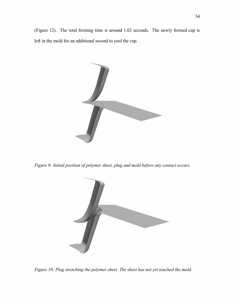
(Figure 12). The total forming time is around 1.02 seconds. The newly formed cup is
left in the mold for an additional second to cool the cup.
Figure 9: Initial position of polymer sheet, plug and mold before any contact occurs.
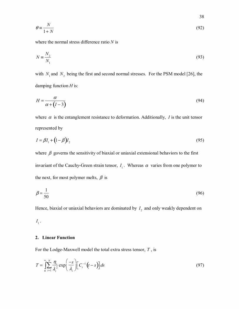
Figure 10: Plug stretching the polymer sheet. The sheet has not yet touched the mold.

35
Figure 11: Screenshot taken as the sheet is inflated. It is no longer touching the plug and just beginning to touch the mold at the top. The total plug contact time is 1.02 s.
Figure 12: Final sheet position just after the after it freezes into position in the mold. The total mold contact time is 0.02 s.

36
The process described above for the simulation matches the manufacturing operation.
The real mold contains several cups thermoformed at once, much like a cupcake pan.
After the thermoforming process is completed with this multi cup mold, the edges must
be cut to create individual cups in a trimming operation. This process is not simulated by
the program, and consists of a die compressing the cup edge at the flat mold surface as it
cuts the circular edge. Figure 7 shows this. Because the edge is compressed, the
measured edge thickness subceeds the simulation’s calculated edge thickness.
C. Viscoelastic Models The nonlinear viscoelastic results use the irreversible Wagner model, which accounts for
the net disentanglement of polymer chains during flow. This induces nonlinearity in the
shear and elongational polymer behaviors. The irreversible Wagner model accurately
describes these behaviors. Linear viscoelastic results are obtained with the special case
called the Lodge-Maxwell model, where no net disentanglement occurs.
1. Nonlinear Function For the Wagner model the viscoelastic component of the total extra stress tensor
component, T , is
T =
11− θ
ηi
λi2
i=1
N
∑0
∞
∫ exp−sλi
H (I1, I2 ) Ct
−1 t − s( )+ θCt t − s( ) ds (85)

37
where i indicates which relaxation modes, with ηi and λi as its corresponding viscosity
and relaxation time; ηi ,λi( ) is called the discrete relaxation spectrum, where λi varies
with temperature, T , as:
λi = aT λid (86) where λid is the discrete relaxation time of the i th mode. Td is the temperature at which
the spectrum was measured [25]. For our polypropylene:
Td = 463K (87)
aT is calculated from the WLF equation, given by
ln aT =
C1 Tr − Td( )C2 + Tr − Td
−C1 T − Td( )C2 + T − Td
(88)
where C1 and C2 are universal WLF constants
C1 = 8.86 KC2 = 101.6 KTr ≡ Tg + 50K
(89)
corresponding to the reference temperature:
Tr ≡ Tg + 50K (90) where
Tg is the glass transition temperature. For polypropylene [25]:
Tg = 263K (91) Furthermore, in Eq. (85) the current time is t and the interval since past time ′t with
respect to t is s . Lastly, Ct is the Cauchy-Green strain tensor, H , the damping function
described below, and θ is a normal stress scalar, defined as
38
θ ≡
N1+ N
(92)
where the normal stress difference ratio N is
N ≡
N2
N1
(93)
with N1 and N2 being the first and second normal stresses. For the PSM model [26], the
damping function H is:
H =
αα + I − 3( ) (94)
where α is the entanglement resistance to deformation. Additionally, I is the unit tensor
represented by
I = β I1 + 1− β( )I2 (95) where β governs the sensitivity of biaxial or uniaxial extensional behaviors to the first
invariant of the Cauchy-Green strain tensor, I1 . Whereas α varies from one polymer to
the next, for most polymer melts, β is
β =
150
(96)
Hence, biaxial or uniaxial behaviors are dominated by I2 and only weakly dependent on
I1 .
2. Linear Function For the Lodge-Maxwell model the total extra stress tensor, T , is
T =
ηi
λi2
i=1
N
∑0
∞
∫ exp−sλi
Ct
−1 t − s( ) ds (97)

39
which is just the Wagner model [(85)] with: H = 1 ; θ = 0 . (98) D. Material Characterization
1. Discrete Relaxation Spectrum The discrete spectrum is composed of five previously measured values Hade and
Giacomin [24] obtained from their rheological measurements at 463 K :
Mode ηi (Pa-s) λi (s) Gi (Pa) 1 216.7 0.000788 275,000 2 1136 0.03792 29,960 3 1549.3 0.1657 9,350 4 1566.5 0.6468 2,422 5 10928.2 6.234 1,753 Table 4: Discrete Spectrum
2. Single Relaxation Time Calculation Letting
Gi ≡
ηi
λi
(99)
define the relaxation modulus of the i th mode, we now let:
G ≡ xi∑ Gi (100) define our average relaxation modulus, where
xi ≡
Gi
G∑ i
≡Gi
GT
(101)
40
so that
G =
Gi2∑
GT
. (102)
We then want η0 for both our single and multiple relaxation time fluids to match. For a Maxwell fluid:
η0 = Gi∑ λi (103) and for our single relaxation time fluid:
η0 = Gλ (104) Combining [(103)] and [(104)] we find the following for our average relaxation time
λ =
Gi∑ λi
G (105)
Combining this with [(102)], we get:
λ =
GT Gi∑ λi
Gi2∑
(106)
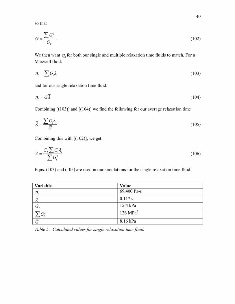
Eqns. (103) and (105) are used in our simulations for the single relaxation time fluid. Variable Value
η0 69,400 Pa-s
λ 0.117 s
GT 15.4 kPa
Gi2∑ 126 MPa2
G 8.16 kPa
Table 5: Calculated values for single relaxation time fluid.
41
E. Plug Heat Transfer Heat transfer to the mold solidifies the part, without affecting its wall thickness
distribution. However, heat transfer to the plug can reshape the part. Plug heat transfer is
implemented by varying the plug temperature, without changing the melt temperature.
The dimensionless temperature difference,θ is
θ ≡
Ts − Tp
Ts − Tm
(107)
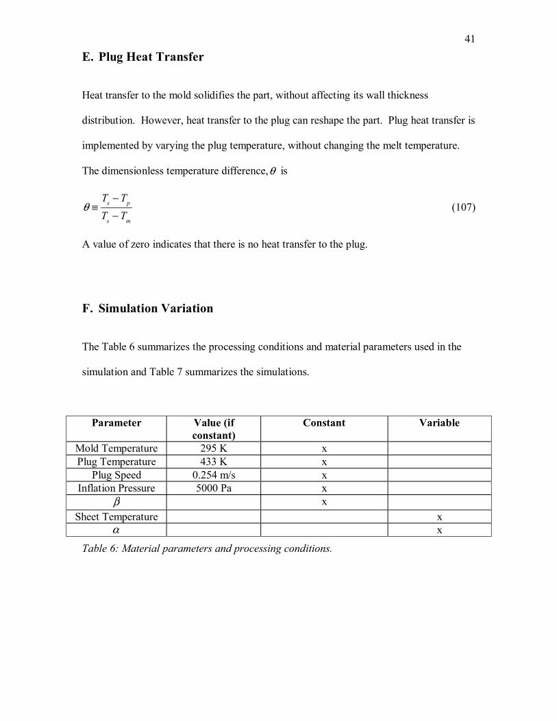
A value of zero indicates that there is no heat transfer to the plug. F. Simulation Variation The Table 6 summarizes the processing conditions and material parameters used in the
simulation and Table 7 summarizes the simulations.
Parameter Value (if constant)
Constant Variable
Mold Temperature 295 K x Plug Temperature 433 K x
Plug Speed 0.254 m/s x Inflation Pressure 5000 Pa x
β x Sheet Temperature x
α x
Table 6: Material parameters and processing conditions.
42
Sim
ulat
ion
#
M
ultip
le
R
elax
atio
n
Sing
le
Rel
axat
ion
Lin
ear
Vis
coel
astic
N
onlin
ear
Vis
coel
astic
α
Plug
T
empe
ratu
re
(K)
θ
β
Plug
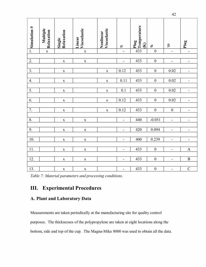
1. x x - 433 0 - - 2. x x - 433 0 - - 3. x x 0.12 433 0 0.02 - 4. x x 0.11 433 0 0.02 - 5. x x 0.1 433 0 0.02 - 6. x x 0.12 433 0 0.02 - 7. x x 0.12 433 0 0 - 8. x x - 440 -0.051 - - 9. x x - 420 0.094 - - 10. x x - 400 0.239 - - 11. x x - 433 0 - A 12. x x - 433 0 - B 13. x x - 433 0 - C
Table 7: Material parameters and processing conditions. III. Experimental Procedures A. Plant and Laboratory Data Measurements are taken periodically at the manufacturing site for quality control
purposes. The thicknesses of the polypropylene are taken at eight locations along the
bottom, side and top of the cup. The Magna-Mike 8000 was used to obtain all the data.

43
A calibration using the Magna-Mike calibration apparatus was performed before each
new measurement for maximum accuracy. In the laboratory additional measurements
were taken along the cup contour with a Magna-Mike 8000. The calibration apparatus
was also used before each new measurement.
B. Method for Comparison of Simulation and Data Because of the cup’s symmetry, only one half of the cup was used for comparison. A
contour was calculated from coordinate locations on the cup for both the simulation and
data. The contour begins at the bottom center of the cup and extends along the centerline
up the wall to the top edge.
IV. Results Figure 13 shows the simulation results using both the single and multiple relaxation
times, as discussed in the methods. These results are compared with process data and lab
measurements, both shown with points.
Figure 13: Simulation comparison with data for discrete spectrum and single relaxation time fluid.
44
The cup center, corner and edge locations are indicated on Figure 8. Along the bottom,
between the center and corner, neither simulation shows a close fit with lab
measurements. The main area of concern is the thinnest area, due to the possibility of
rupture. For thermoformed cups, the thinnest part is the corner. Here both simulations
are accurate. Along the sidewall both simulations over estimate thickness, however the
single relaxation time fluid is the closest to data. Edge thickness for the simulations and
process data disagrees by as much as 21 percent of the simulation edge thickness. This is
due to the cutting operation, which compresses the initial material thickness and is not
simulated with our finite element program. Overall, the single relaxation fluid fits the
data at more points than the spectrum. Because the single relaxation time fluid is the most
accurate we will use it to improve the existing process to obtain a larger minimum
thickness and improve thickness uniformity along the cup bottom.
The accuracy of the single relaxation time fluid simulation is exciting. Whereas the
spectrum consumed 8011.6 sec of CPU time, the single relaxation time computation
consumed only 7166.1 sec. For more complicated shapes, bigger savings in computation
time are expected. Furthermore, the use of single relaxation time fluids allows us to
easily adimensionalize simulation results. Defining the Deborah and Weissenberg
numbers, for example, is straightforward.
To improve the simulation’s thickness uniformity at the bottom and sidewall areas, as
well as to increase the minimum thickness, we have modified plug temperature, plug
draw depth, and polymer entanglement resistance. Left to its own devices, the plug
temperature will eventually reach a steady state, matching the melt temperature. If we
45
control the plug temperature, then raising it will transfer heat to the melt during plug
assist. The heat transfer between the mold and sheet will always be insignificant because
the polymer sheet freezes into place immediately upon contact with the mold. For this
analysis the single relaxation time simulation was modified, because it had the best fit
from Figure 13. Furthermore, the original single relaxation time simulation is displayed
to detect any differences for new simulations. θ is the heat transfer value as described in
the Methods section.
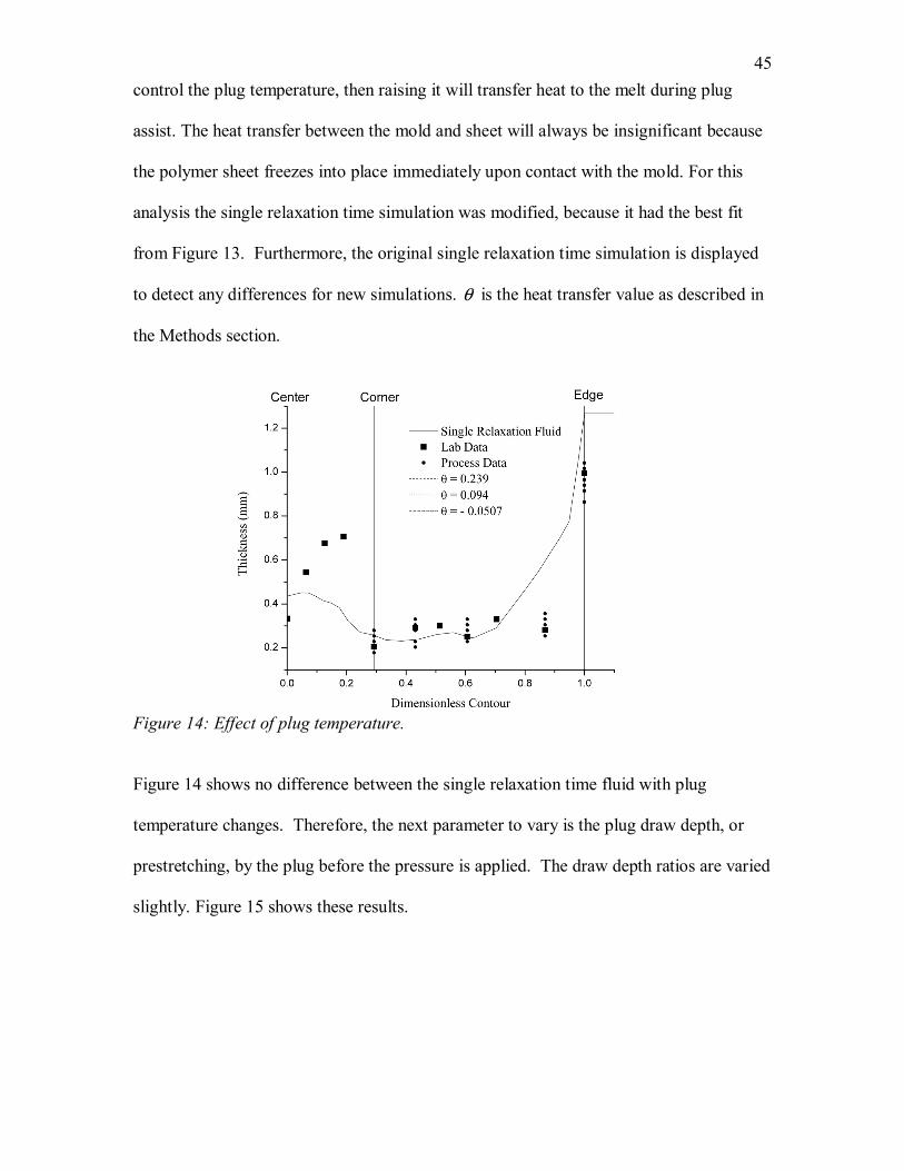
Figure 14: Effect of plug temperature.
Figure 14 shows no difference between the single relaxation time fluid with plug
temperature changes. Therefore, the next parameter to vary is the plug draw depth, or
prestretching, by the plug before the pressure is applied. The draw depth ratios are varied
slightly. Figure 15 shows these results.

46
Figure 15: Effect of draw depth ratio.
As the draw depth increases from Plug A to Plug C, the sidewall area between the corner
and edge decreases in thickness. The extra sheet material is pushed to the bottom
between the center and corner. Also, the minimum thickness is increased as the draw
depth increases.
The previous simulations have concentrated on the linear viscoelastic behavior. It is also
necessary to explore the nonlinear viscoelastic behavior. This introduces a more
complicated model, as described in the Methods. Figure 16 allows the exploration of
changing the α to change the network strand’s ability to resist deformation. A larger α
value indicates an increased resistance.
Single Relaxation Fluid

47
Figure 16: Effect of α for viscoelastic cases: nonlinear versus linear.
Overall, additional deformation resistance decreases the simulation accuracy. The linear
model of the single relaxation time fluid is still the most accurate. This is especially
evident at the sidewall between the corner and edge, and the bottom between the center
and corner. As α decreases , the sidewall thickness and minimum thickness value
decreases. Furthermore, edge thickness for the simulations and process data disagrees by
as much as 21 percent. This is likely due to the difference between the processing
simulation and the actual thermoforming process.
Figure 17 allows the exploration of changing the β to change the material’s extensional
behavior to I1 . A larger β value increases I1 .

48
Figure 17: Simulation results from the β values for nonlinear viscoelastic.
Overall, the addition of extensional behavior to I1 decreases the simulation accuracy.
The linear model of the single relaxation time fluid is still the most accurate. This is
especially evident at the sidewall between the corner and edge, and the bottom between
the center and corner. As β decreases , the sidewall thickness and minimum thickness
value decreases. Furthermore, edge thickness for the simulations subceeds the process
data by as much as 21%.
V. Discussion Because Figure 13 uses the actual processing conditions from the manufacturing
environment, these results are used to validate the capability of this finite element
program as method to predict the thickness distributions. Overall, the simulation follows
the general pattern of the measured values and shows a desirable fit to measured values
of the data points. This result validates the use of this finite element program to predict
49
the outcome of this specific cup thermoforming process. The literature also shows that
finite element simulation provide good approximations to measured thicknesses for
similar vacuum formed cross sections.
The simplified model of the single relaxation time fluid has a better fit to the data for a
majority of the points, especially at the sidewall, corner and edge. Therefore, this is the
best method characterize the polypropylene. This type of analysis has not been
investigated in the literature. Previous literature has only analyzed the effect of
processing conditions such as sheet temperature, mold temperature and the duration of
pressure application.
Figure 13 also indicates that processing conditions used in the initial simulation are
correct. Therefore, the rest of the simulations concentrate on improving upon the initial
process by altering processing parameters. Therefore, because the initial material
characterization and processing conditions are validated, any improvements shown by the
simulations are accurate.
The variation of plug temperature has no effect on the thickness distribution of the linear
material model. Results of previous by Lee [23] of reverse vacuum prestretching found
that sheet thickness distribution changed with mold temperature for the nonlinear
material model. These results showed that small variations in sheet temperature, on the
order of 20ºC, altered the thickness throughout the entire cross section. The largest
alterations occurred at the corners and throughout the bottom. It is possible that the plug
negates any effects of sheet temperature. It would be interesting to investigate this
possibility in further studies.
50
Increasing draw depth changes the location along the contour of the thinnest point and
increases the minimum thickness value. As a result the sheet thickness uniformity
improves with increasing draw depth, resulting in fewer stress concentrations because of
smaller variations in thickness. Additionally, the possibility of the sheet to develop holes
decreases. Increases in draw depth also push more material to the bottom while thinning
the sidewall. This shows the importance of draw depth for modifying the thermoforming
operation to control the amount of thinning on the sidewall. The result matches the
accepted theory of plug assist very closely [4]. The most accurate simulation to the
process and lab data is the single relaxation time fluid with the deepest draw depth.
VI. Conclusion The evidence suggests that a single time fluid should be used to characterize the
polypropylene in simulations. Furthermore, altering the processing conditions to include
a deeper draw depth will improve cup thickness uniformity and minimum sheet
thickness. Lastly because, heat transfer between the plug and the sheet has no effect on
the thickness distribution, there is no concern for unstable processing conditions due to
temperature changes in the sheet or plug. Therefore, the process can be characterized as
reliable and consistent.
VII. Acknowledgement
The authors are indebted to Dr. Jaydeep Kulkarni of Fluent Corporation for his technical
guidance with the finite element software, and to Dr. Martin Stephenson of the Placon
Corporation for his technical advice. We thank the Placon Corporation of Madison,

51
Wisconsin and Plastic Ingenuity, Inc. of Cross Plains, Wisconsin for their financial
support through their memberships in the Industrial Consortium of the Center for
Advanced Polymer and Composite Engineering at the University of Wisconsin. The
Placon Corporation is also recognized for its sustaining sponsorship of the Rheology
Research Center of the University of Wisconsin. Kershner is also indebted to the Society
of Plastics Engineers for a scholarship awarded by the Thermoforming Division.

52
References [1] Tadmor, Z. and Gogos, G.G., Principles of Polymer Processing, John Wiley & Sons, Inc., New York (1979). [2] Hart-Smith, L.J. and Crisp, J.D.C., Int. J. Eng. Sci., 5, 1(1967). [3] Sheryshev, M.A., Zhogolev, I.V. and Salazkin, K.A., Soviet Plast. , 11, 30 (1969). [4] Williams, J.G., J. Strain Analysis, 5, 49 (1970). [5] Rosenzweig, N., Narkis, M. and Tadmor, Z., Polymer Engineering and Science, 19, 946 (1979). [6] Throne, J.L., Plastics Process Engineering, Marcel Dekker, New York (1979). [7] Pearson, J.R.A., Mechanics of Polymer Processing, Elsevier Applied Science Publishers Ltd., London (1985). [8] Allard, R., Charrier, J.-M., Ghosh ,A., Marangou, M., Ryan, M.E., Shrivastava, S. and Wu, R., J. Polym. Eng., 6, 363 (1986). [9] Baird, D.G. and Collias, D.I., Polymer Processing Principles and Design, Butterworth-Heinemann, Boston (1995); Wiley & Sons, New York (1998). [10] Osswald, T.A. and Hernández-Ortiz, J.P., Polymer Processing - Modeling and Simulation, Hanser Publishers, Munich (2006). [11] Strong, A.B., Plastics Materials and Processing, 3rd ed., Prentice Hall, Upper Saddle River, New Jersey (2006). [12] Bird, R.B., Armstrong, R.C. and Hassager, O. , Dynamics of Polymeric Liquids, Vol. 1: Fluid Mechanics, 2nd ed., Wiley & Sons, New York (1987); see Eq. (8.4-15). [13] Stephenson, M.J., Dargush, G.F. and Ryan, M.E., Polymer Engineering and Science, 39, 2199 (1999). [14] Stephenson, M.J., An Experimental and Theoretical Study of Sheet Sag in the Thermoforming Process, PhD Thesis, State University of New York, Buffalo, NY (August 1997).

53
[15] Rosenzweig, N., Narkis, M., Tadmor, Z., “Wall Thickness Distribution in Thermoforming”, Polymer Engineering and Science, 19, 946-951(1979) [16] Charrier, J.-M., Shrivastava, S. “Free and Constrained Inflation of Elastic Membranes in Relation to Thermoforming-Non-Axisymetric Problems”, Journal of Strain Analysis, 24, 35-72 (1979) [17] Throne, J.L.“Modelling Plug-assisted Thermoforming”, Advances in Polymer Technology, 9, 309-320 (1989) [18 ] Song, W.N., Mirza, F.A., Vlachopoulous, J., “Finite Element Simulation of Plug-assist Forming”, International Polymer Processing, 7, 248-256 (1992) [19] DeLorenzi, H.G., Nied, H.F., Taylor, C.A., “A Numerical/Experimental Approach to Software Development for Thermoforming Simulations”, Journal of Pressure Vessel Technology, 113, 102-114 (1991) [20] Nied, H.F., Taylor, C.A., DeLorenzi, H.G., “Three-Dimensional Finite Element Simulation of Thermoforming”, Polymer Engineering and Science, 30, 1314-1322 (1990) [21] Erchiqui, F., Gakwaya, A., Rachik, M., “Dynamic Finite Element Analysis of Nonlinear Isotropic Hyperelastic and Viscoelastic Materials for Thermoforming Applications”, 45, 125-134 (2006) [22] Erchiqui, F., Thermodynamic Approach of Inflation Process of K-BKZ Polymer Sheet With Respect to Thermoforming”, Polymer Engineering and Science, 45.1319-1335 (2005) [23] Lee, J.K., Virkler, T.L., Scott, C.E., “Effects of Rheological Properties and Processing Parameters on ABS Thermoforming”, Polymer Engineering and Science, 41, 240-261 (2001) [24] Hade, A.J., Giacomin, A. Jeffrey, “Characterization of Thermoforming Resins Using Exponential Shear”, Proc. XIVth Int. Congr. On Rheology, 1-3 (2004) [25] Osswald, T., Menges, G., “Materials science of polymers for engineers”, Hanser Publishers , Munich (2003) [26] Dealy, J., Wissbrun, K., “ Melt rheology and its role in plastics processing: theory and applications”, Van Nostrand Reinhold, New York (1990)