mee#ng&of&the&steering&group&on&simula#on&(sgs ... action/gge_ldv... ·...

Mee#ng of the Steering Group on Simula#on (SGS)

Sensi#vity analysis of the Cruise model Methods, Tools and Boundaries

Brussels, 02 April 2014

B. Ciuffo , G. Fontaras, S. Tsiakmakis, A. Maro7a

Objective

2

•  A model is usually based on several (dozens to hundreds) inputs and parameters.

•  Their effect on the different outputs can be very different and only a few have usually a significant effect on a specific one.

•  The WLTP/NEDC correlation function needs to be based on the most important input parameters

•  A proper parameter selection is crucial. •  The approach proposed for this selection is based

on the Sensitivity Analysis of the Cruise model

Family of theories and techniques aimed at defining how “the uncertainty in the model outputs can be apportioned to

the different sources of uncertainties in the model inputs”

Important to:

•  uncover technical errors in the model

•  identify critical regions in the inputs domain

•  simplify models

Additional advantage

•  Possibility to foresee the inaccuracy due to parameters not allowed to vary (e.g. engine maps, etc.)

Global sensitivity analysis

3

4

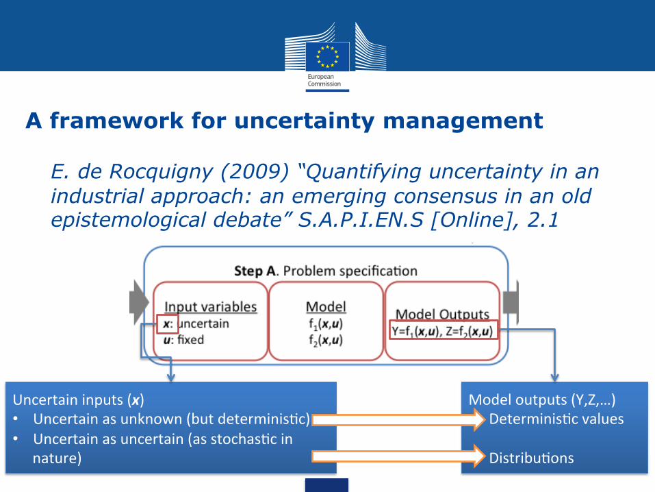
A framework for uncertainty management

E. de Rocquigny (2009) “Quantifying uncertainty in an industrial approach: an emerging consensus in an old epistemological debate” S.A.P.I.EN.S [Online], 2.1

4

Uncertain inputs (x) •  Uncertain as unknown (but determinisBc) •  Uncertain as uncertain (as stochasBc in

nature)

Model outputs (Y,Z,…) •  DeterminisBc values

•  DistribuBons

5

Uncertainty management

The process of identification/quantification/reduction of model uncertainties (different from accuracy)

Variance-based approach to GSA

6

•  Output variance as a proxy of output uncertainty •  Variance decomposition formulas as sensitivity analysis

tools •  Pros:

•  Very Accurate for analytic models (analytic evaluation of the variances) or for computationally inexpensive models (to allow huge numbers of model evaluations)

•  Cons: •  Accuracy connected to the number of simulations allowed for

computationally expensive models •  Need an accurate definition of the problem settings (careful

identification of input ranges, distributions and correlation structure of the model)

Variance-based methods (Cukier, 1973; Sobol, 1990; Homma and Saltelli, 2000)

7

Y Y

X2 X1

Y=f(X1,X2)

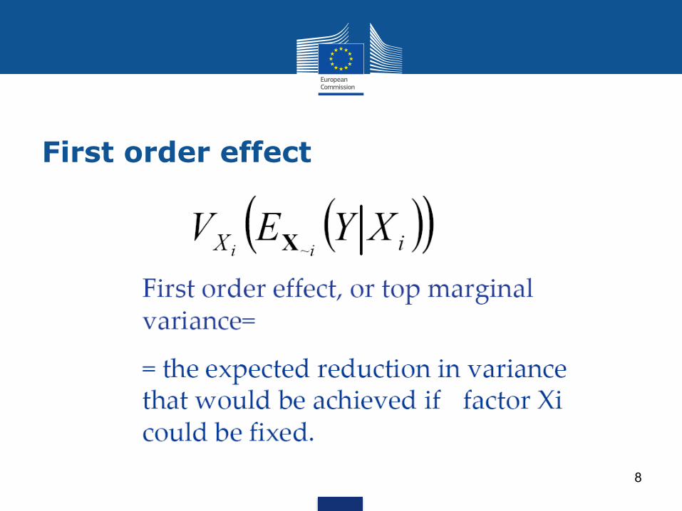
First order effect

8

Variance decomposition

9

Sobol sensitivity indices

10

An efficient (numerical) evaluation of Sobol indices requires the application of techniques based on QMC methods (Saltelli et al. 2012)

Evaluation of variances requires the calculation of multi-dimensional integrals Since the analytical formulation of Cruise is not available, a Monte-Carlo-based numerical approach can be used

Quasi-Monte Carlo Simulation Plan

11

Monte Carlo framework using Sobol quasi-random sequences: “Quasi Monte Carlo” methods

If the sequence of random numbers keeps “low-discrepancy” whatever the number of dimensions, the size of the Monte Carlo experiment decreases Discrepancy: a measure of deviation from uniformity Prof. I.M.Sobol has devoted big part of his life in studying LDS properties

Some properties of Sobol sequences (1)

12

Some properties of Sobol sequences (2)

13

In integral calculation, error ε: Sobol sequence (for N=2k) Other LDS

Random numbers

Sensitivity analysis of Cruise

14

1.  Select a vehicle configuration 2.  Identify the relevant Cruise parameters 3.  Define ranges of variability for each parameter and the

correlations among them 4.  Design a simulation plan for the evaluation of the

sensitivity indices 5.  Perform the simulations 6.  Check for unfeasible combinations 7.  Evaluate the sensitivity indices 8.   Rank parameters on the basis of their effect 9.   Define influential vs. non-influential threshold

Steps of the Cruise SA - 1

15

•  Selection of a baseline vehicle configuration: •  Gasoline conventional vehicle •  Manual transmission •  Start-stop system the only additional technology


16

•  Selection of vehicle parameters: •  For the time-being Cruise “calibration” parameters

not taken into account (e.g. cold-start effect) •  Difficult to define ranges and correlations for them

•  No electrical components considered •  Parameters correlations derived from available

information

17

Steps of the Cruise SA – 3. Overview


•  The boundaries are connected to the specific sampling strategy •  A first sample is made from the range reported using Sobol quasi

random numbers and assuming uniform distribution

Parameter Abbreviation LB UB IntegerDisplacement5param. cc 0 1 NoPower5param. P 0 1 NoRated5RPM5param. rRPM 0 1 NoIdle5RPM iRPM 650 1250 YesMass5in5running5order5(NEDC)5param. Mn 0.6 1.4 NoRandom5factor5for5WLTP5mass N1 0 1 NoEngine5inertia5param. eI 0.8 1.2 NoCd*A5in5aerodynamic5resistance aR 0 1 NoFR05in5rolling5resistance5param. fR0 0 1 NoRandom5factor5for5WLTP5rolling5resistance N2 0 1 NoRandom5factor5for5WLTP5aerodynamic5resistance N3 0 1 NoMax5speed5param. maxV <15 15 NoStartLstop sS 1 1 YesEngine5map5(w5or5w/o5turbo) eM 0 1 YesGear5box5sample5parameter gB 1 50 YesFR15in5rolling5resistance5param. fR1 0 1 No

0.00#

0.10#

0.20#

0.30#

0.40#

0.50#

0.60#

0.70#

0.80#

0.90#

1.00#

0# 1000# 2000# 3000# 4000# 5000# 6000# 7000# 8000# 9000#Displacement,(cc),

Displacement,cdf,

The sampling strategy

19

•  Consistently with the fleet segmentation criteria used in the project, key independent variable in the sampling is the engine displacement

•  The corresponding parameter “cc” is uniformly sampled in the range [0,1]

•  The displacement to use in the simulation is then derived inverting the cdf (EEA, 2013)

cc

2. Engine power

20

Middle&line&:&y&=&0.0699x&0&13.282&R²&=&0.8532&

0&

50&

100&

150&

200&

250&

300&

350&

700& 1200& 1700& 2200& 2700&

Engine

&Pow

er&(k

W)&

Capacity&(cc)&

Engine&type&&A&(low&P&per&CC&eg&non&turbo)&Engine&type&&B&(high&eng&P&per&CC&eg&turbo)&

variaKon&

limits&

•  Engine power is derived from displacement (EEA, 2013). From the joint distribution 2 types of engines are considered*: with and without turbo

•  The parameter eM {0,1} is used to choose the type •  The parameter P [0,1] is used to find the correct

engine power to use in simulation

* The 2 regions have been defined using the regression line as basis. Additional data are required to perform a more appropriate differentiation

Displacement

eM

P

3. Rated RPM

21

•  Rated RPM is sampled from a triangular* distribution having the following coeff. a=4500 b=9000 c=5000 Values of rated RPM in the range [4900-5500] have the highest probability to be selected

•  The parameter rRPM [0,1] is used for the sampling

* We choose a triangular distribution being the simplest skewed distribution. Other options can be used (e.g. Normal skewed, etc.)

rRPM

4. Idle RPM

22

•  The value for idle RPM is directly taken from the parameter iRPM which has been sampled from a uniform distribution based on the range [650,1250]

5. NEDC mass

23

•  Vehicle mass is connected to displacement with the data available from EEA (2013)

•  The mass dispersion identified by the parameter Mn [0.6,1.4] is applied to the value achieved

•  The NEDC mass is then used for the inertia class determination

y"="626.84ln(x)"."3253.1"R²"="0.67281"

0"500"1000"1500"2000"2500"3000"3500"4000"4500"5000"

0" 1000" 2000" 3000" 4000" 5000" 6000" 7000" 8000"

Mass$(kg)$

Capacity$(cc)$

varia:on"limits"

Displacement

Mn

6. Test mass WLTP

24

•  Simplified approach here: from the available data it has been estimated that the coefficient between NEDC and WLTP masses (α) follows a N(1.15,0.03) distribution*

•  The value sampled for the parameter N1 [0,1] is used to evaluate the mass coefficient by inverting the Normal distribution

•  WLTP mass is obtained accordingly •  MWLTP=αMNEDC

* Also in this case, other approaches can be used and will be tested

7. Engine Inertia

25

•  From the available data it has been found that engine inertia is linearly correlated with engine displacement by the following relationship*: •  Inertia=0.27Displacement(l)+0.31

•  A 20% variation is considered and is derived from the parameter eI [0.8,1.2] •  Inertia=(0.27Displacement(l)+0.31)eI

* This relationship has been taken from the HDV sector. Its suitability to the LDVs must be verified

8. Max Vehicle Speed

26

•  The maximum vehicle speed is obtained from the data made available by Heinz Steve

•  MaxSpeed=46.34�Power0.319

•  A ±15km/h variability is added using the parameter mV [-15,15]

y"="46.339x0.319"R²"="0.88509"

0"

50"

100"

150"

200"

250"

300"

350"

400"

0" 100" 200" 300" 400" 500" 600"

V"max"(k

m/h)"

Power"(kW)"

cars,"Petrol"

KBA statistics 2009 (source Heinz Steven) "

Outliers"not"considered"(speed"limiCng"effect)"

Power

mS

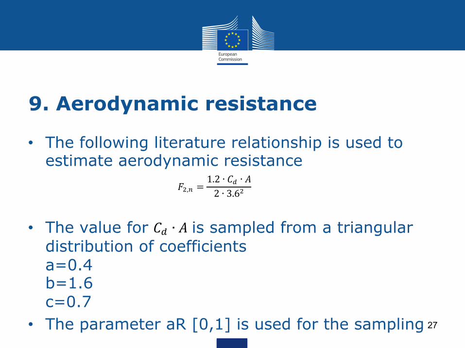
9. Aerodynamic resistance

27

•  The following literature relationship is used to estimate aerodynamic resistance

•  The value for is sampled from a triangular distribution of coefficients a=0.4 b=1.6 c=0.7

•  The parameter aR [0,1] is used for the sampling

!!,! =1.2 ∙ !! ∙ !2 ∙ 3.6!

!! ∙ !

10. Rolling resistance (F0)

28

•  The following literature relationship is used to estimate rolling resistance (F0)

•  The value for fR0 is sampled from a Normal distribution N(0.0081,0.002)

•  The value of the parameter fR0 [0,1] is used for the sampling

!!!,! = !!! ∙ ! ∙!!"#$

11. Rolling resistance (F1)

29

•  The following literature relationship is used to estimate rolling resistance (F0)

•  The value for fR1 is sampled from a Normal distribution N(0.00006,0.000015)

•  The value of the parameter fR1 [0,1] is used for the sampling

!!!,! =!!! ∙ ! ∙!!"#$

3.6

12. WLTP RLs

30

•  In order to take into account the variability in the RLs, from the available data, it was estimated that the correlation between WLTP and NEDC RLs follow the following distributions: N(1.4,0.1) (for F0 and F1) N(1.05,0.01) (for F2)

•  The parameters N2 and N3 [0,1] are used for the sampling

13. Gear-box definition (Draft)

31

•  Since the correlation between gear-box parameters and the other parameters was of difficult estimation, the following approach is considered

•  A range for each input to the GB-tool (JRC) was assigned.

•  A set of rules was defined to see if a combination of inputs could lead to a realistic or not realistic gear-box


32

•  Using Sobol numbers, 106 input combinations were defined

•  Among those, around 150.000 resulted plausible •  These 150.000 were used as input for the SA

Parameter Abbreviation LB UBGearbox2size gS 4 7Gear2ratio21st2gear gR1 3 5Gear2ratio2last2gear2no2overdrive2considered gRl 0.3 2Final2drive fD 2 6Overdrive2(02or21) ov 0 1Overdrive2ratio ovR 0.4 1Rated2RPM rRPM 3000 10000Idle2RPM iRPM 6200 200RPM2@Vmax vRPM 61000 1000Top2Speed tS 120 250R2dyn R 0.2 0.4P2max P 25 200Fuel2(02or21) F 0 1Max2Laden2Mass mLm 1000 3000F0 F0 0 200F1 F1 0 1F2 F2 0 0.1Max2slope2for2start mSs 20 50Max2torque mT 20 100f2 f2 0.5 1.5f2tunning fT 60.25 0.25Parameter2to2fix212between2gRl,2tS,2and2R2to20 c 1 3

Parameters common to gear-box and vehicle simulation

Relations used for input sampling

34

ConstraintsfT=fT+0.7*f2+0.45F2=min(F2,0.263:0.00093*tS)iRPM=iRPM+2.9*fD^3:60*fD^2+460*fD:200gRl=max(gRl,gR1/8,2:2*fT)ifIc==1,IgRl=0ifIc==2,ItS=0ifIc==3,IR=0vRPM=vRPM+rRPM


35

•  8 parameters are common to the two simulation plans: {P,rRPM,iRPM,maxV,M,F0,F1,F2}

•  Per each of their combination in the simulation plan for the SA, the distance with respect to any of the 150.000 combinations among the plausible gear-boxes was evaluated:

•  The 50 closest “plausible gear-boxes” are selected

Dj =Pi,V −Pi,GB, j

Pi,V

"

#$$

%

&''

2

i=1

8

∑


36

•  The gear-box to be used in simulation is that sampled from the sub-set of the 50 closest gear-boxes using the variable gB [1,50]

•  Although somehow “elaborate”, this approach would allow examine the variability of gear-box/vehicle combinations in details

•  To see if really necessary. Possible alternatives under discussions.

•  Inputs from SGS?

14. Start-stop

37

•  The simple SS system implemented in CRUISE is activated depending on the value of the variable sS {0,1}

Capacity and RPM rescaling: Willan fitting approach

38

•  Literature based simplified model:

Pme = [ea (Cm) – eb(Cm) x Pma] x Pma – Pmloss (Cm)

•  Which can be expanded as follows:

ea (Cm) = ea1 + ea2 x Cm + ea3 Cm^2

eb (Cm) = eb1 + eb2 x Cm

Pmloss (Cm) = Pme0 (0) + Pme01 x Cm^2

•  Least squares fitting leads to the description of the map with 7 parameters: (ea1, ea2, ea3, eb1, eb2, Pme0(0), Pme01)

•  Rescaling of the engine map is now direct as it becomes a function of mean piston speed (thus capacity and rpm are considered) - For more details check JRC’s specific presentation

Simulations-Next steps

39

•  A first run of simulations was carried out to check the results

•  Some issues still need to be addressed (especially on the gear-box)

•  A first SA will be run also basing on the outcomes of the meeting (and on the support by OEMs)

•  Other vehicle simulation inputs will be considered as well as additional technology packages as more element will be available

Conclusions

40

•  A first plan for the SA of Cruise has been developed.

•  The sampling strategy adopted tried to consider the highest possible variation in the space of the model inputs, though trying to limit the analysis to meaningful combinations

•  Inputs from OEMs in providing input data for the analysis is very important!

mee#ng&of&the&steering&group&on&simula#on&(sgs ... action/gge_ldv... ·...

Documents