mechanistic investigation of catalytic organometallic
TRANSCRIPT

Mechanistic investigation of catalytic organometallic reactions using ESI MS
by
Jingwei Luo
M.Sc., Queen’s University, 2009
M.Sc., Minzu University of China, 2007
B.Sc., Minzu University of China, 2004
A Dissertation Submitted in Partial Fulfillment
of the Requirements for the Degree of
DOCTOR OF PHILOSOPHY
in the Department of Chemistry
© Jingwei Luo, 2014
University of Victoria
All rights reserved. This dissertation may not be reproduced in whole or in part, by photocopy or
other means, without the permission of the author.

ii
Supervisory Committee
Mechanistic investigation of catalytic organometallic reactions using ESI MS
by
Jingwei Luo
M.Sc., Queen’s University, 2009
M.Sc., Minzu University of China, 2007
B.Sc., Minzu University of China, 2004
Supervisory Committee
Dr. J. Scott McIndoe, Department of Chemistry
Supervisor
Dr. Lisa Rosenberg, Department of Chemistry
Departmental Member
Dr. Frank van Veggel, Department of Chemistry
Department Member
Dr. Laurence Coogan, Department of Earth and Ocean Science
Outside Member

iii
Abstract
Supervisory Committee
Dr. J. Scott McIndoe, Department of Chemistry
Supervisor
Dr. Lisa Rosenberg, Department of Chemistry
Departmental Member
Dr. Frank van Veggel, Department of Chemistry
Department Member
Dr. Laurence Coogan, Department of Earth and Ocean Science
Outside Member
Electrospray ionization mass spectrometry (ESI-MS) has been applied to the real time study of
air-sensitive homogenous organometallic catalytic reactions due to its soft ionization properties.
Therefore, fragile molecules and complexes in these reactions were characterized. The kinetic
studies of these reactions have also been done by following the relative abundance of different
species including starting material(s), products, by-product(s) as well as intermediates. Based on
the results, reaction pathways and mechanisms were proposed and numerical models were built
to accurately mimic the reactions under specific condition.
In order to make the reactions detectable by ESI-MS, many charged ESI-MS friendly substrates
were synthesized as tracking tags, including 1-allyl-1-(prop-2-yn-1-yl)piperidin-1-ium
hexafluorophosphate(V), 1-allyl-1-(prop-2-yn-1-yl)pyrrolidin-1-ium hexafluorophosphate(V),
(4-ethynylbenzyl)triphenylphosphonium hexafluorophosphate(V), hex-5-yn-1-
yltriphenylphosphonium hexafluorophosphate(V) etc. The method for continuously monitoring
water- and oxygen-sensitive reactions in real time named pressurized sample infusion (PSI) was
developed, optimized and applied throughout all the projects in the thesis.
These techniques were applied to detailed studies of the intramolecular Pauson-Khand reaction
(PKR) with Co2CO8 under different temperatures. The kinetic study results gave the entropy and

iv
enthalpy of the reaction and evidence suggested that the ligand dissociation step was the rate-
determining step of the reaction.
Hydrogenation of alkynes with Wilkinson’s catalyst and Weller’s catalyst were also studied
using PSI. The behaviour of starting materials and products were tracked, then various reactions
were carried out by using different temperatures and concentrations. Furthermore, competition
reaction and kinetic isotope effect study, mechanisms were proposed based on experimental
results, numerical models were built, and rate constants for each step were estimated.
Different Si-H activation reactions were studied including hydrolysis of silanes, hydrosilation,
dehydrocoupling of silanes, alcoholysis of silane and silane redistribution by using (3-
(methylsilyl)propyl)triphenylphosphonium hexafluorophosphate(V). A variety of collaborative
projects were also carried out including hydroacylation, fast-activating Pd catalyst precursor,
catalyst analysis for Cu-mediated fluorination, CdSe - NiDHLA analysis, Ru catalyzed
propargylic amination reaction, Zn catalyzed lactide polymerization, and Fe4S4 clusters.
v
Table of Contents
Supervisory Committee .................................................................................................................. ii Abstract .......................................................................................................................................... iii Table of Contents ............................................................................................................................ v
List of Tables ................................................................................................................................ vii List of Schemes ............................................................................................................................ viii List of Figures ................................................................................................................................ ix List of Abbreviations ................................................................................................................... xvi List of Structures ........................................................................................................................ xviii
Acknowledgments....................................................................................................................... xxii Dedication .................................................................................................................................. xxiii
1. Literature Review........................................................................................................................ 1
1.1 Organometallic catalysis ................................................................................................. 1 1.2 Traditional methods for analysis of organometallic reactions ........................................ 4
1.2.1 NMR Spectroscopy ..................................................................................................... 5 1.2.2 UV/Vis Spectroscopy................................................................................................ 11
1.2.3 IR Spectroscopy ........................................................................................................ 13 1.2.4 Mass Spectrometry.................................................................................................... 16
2. Techniques and methodologies ................................................................................................. 25 2.1 Introduction ................................................................................................................... 25 2.2 Electrospray Ionization Mass Spectrometry ................................................................. 26
2.3 Quadrupole –Time of Flight (Q-TOF) .......................................................................... 29 2.4 Continuous reaction monitoring with ESI-MS ............................................................. 33
3. Methodological innovations...................................................................................................... 37
3.1 Numerical modeling...................................................................................................... 37
3.2 Powersim model design ................................................................................................ 41 3.3 Handling air and moisture sensitive reactions .............................................................. 46
3.4 PSI-ESI-MS optimization ............................................................................................. 48 3.4.1 PSI-ESI-MS filter...................................................................................................... 48 3.4.2 PSI-ESI-MS dilution system ..................................................................................... 50
3.4.3 PSI glassware ............................................................................................................ 51 4. The Pauson-Khand Reaction ..................................................................................................... 54
4.1 Introduction ................................................................................................................... 54
4.2 Selected studies ............................................................................................................. 56 4.3 Challenges of ESI-MS for Pauson-Khand studies ........................................................ 57 4.4 Advantages of ESI-MS for the Pauson-Khand Reaction studies .................................. 58
4.5 Results and Discussion ................................................................................................. 59 4.5.1 Design of charged substrate ...................................................................................... 59 4.5.2 Synthesis of cobalt complexes .................................................................................. 60 4.5.3 Previous gas phase reaction ...................................................................................... 62
4.5.4 Intramolecular Pauson-Khand reaction ..................................................................... 63 4.6 Conclusion .................................................................................................................... 68
4.7 Experimental ................................................................................................................. 68 5. Detailed kinetic analysis of rhodium-catalyzed alkyne hydrogenation .................................... 75
5.1 Hydrogenation of olefins by Rh (PPh3)3Cl ................................................................... 75
vi
5.1.1 Introduction ................................................................................................................... 75 5.1.2 Previous investigation with ESI-MS ......................................................................... 78
5.1.3 Results and Discussion ............................................................................................. 80 5.1.4 Conclusion ................................................................................................................ 92
5.2 Hydrogenation of olefins by Weller’s catalyst ............................................................. 93 5.2.1 Introduction ............................................................................................................... 93 5.2.2 Results and Discussion ............................................................................................. 94
5.2.3 Conclusion .............................................................................................................. 109 5.3 Experimental ............................................................................................................... 109
6. The use of charged substrates to investigate Si-H activation by ESI MS ............................... 113 6.1 Current research in the area of Si-H activation ........................................................... 113
6.1.1 Dehydrocoupling of silane ...................................................................................... 113
6.1.2 Hydrolysis of silanes ............................................................................................... 118
6.1.3 Hydrosilation........................................................................................................... 120
6.2 Results and Discussion ............................................................................................... 122 6.3 Future work ................................................................................................................. 132
6.4 Experimental ............................................................................................................... 133 7. Collaborative studies ............................................................................................................... 135
7.1 CdSe-DHLA for H2 production .................................................................................. 135 7.2 Fe4S4 clusters .............................................................................................................. 137 7.3 Lactide polymerization by cationic zinc complexes ................................................... 140
7.4 Copper-Mediated Fluorination of Arylboronate Esters. Identification of a Copper(III)
Fluoride Complex ................................................................................................................... 142
7.5 Ti, Hf and Zr complexes ............................................................................................. 143 7.6 Unusually Effective Catalyst Precursor for Suzuki−Miyaura Cross-Coupling Reactions
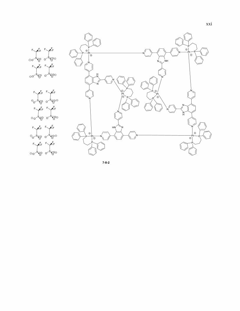
…...………...……..……...………………………….....……………………………..145 7.7 Rhodium complexes catalyzed hydroacylation reaction............................................. 148 7.8 CryoSpray MS (CSI-MS) ........................................................................................... 152
8. Conclusion .............................................................................................................................. 155 References ................................................................................................................................... 157
Appendix A: Intermediate data for Pauson-Khand reaction ....................................................... 165
Appendix B: Numerical modeling, rate constants and ESI-MS data for hydrogenation reactions
..................................................................................................................................................... 166
Appendix C: Crystal data and structure refinement for PPh3P(CH2)4CCH .............................. 170 Appendix D: Crystal data and structure refinement for PPh3P(CH2)5CH3. ................................ 178 Appendix E: Crystal data and structure refinement for (4-ethynylbenzyl)triphenylphosphonium
hexafluorophosphate(V). ............................................................................................................ 188 Appendix F: Supporting data for Weller’s hydrogenation ......................................................... 205
Appendix G: Crystal data and structure refinement for PPh3P(CH2)5CH3. ................................ 209 Appendix H: Data for collaboration projects .............................................................................. 217
vii
List of Tables
Table 1: Ferrocenyl polyphosphanes structures and decoupled proton 31
P NMR data19
. Reprinted
with permission from “Congested Ferrocenyl Polyphosphanes Bearing Electron-Donating or
Electron-Withdrawing Phosphanyl Groups: Assessment of Metallocene Conformation from
NMR Spin Couplings and Use in Palladium-Catalyzed Chloroarenes Activation” S. Mom, M.
Beaupérin, D. Roy, S. Royer, R. Amardeil, H. Cattey, H. Doucet and J. C. Hierso, Inorganic
Chemistry, 2011, 50, 11592-11603. Copyright © 2011 American Chemical Society ................... 8
Table 2: Filter performance table .................................................................................................. 50
Table 3: Aggregates and species in the reaction solution: ............................................................ 72
Table 4: Rate constants for the numerically modelled reaction at 23°C....................................... 90
Table 5: Estimated rate constants by different COPASI methods. First order rate constants are in
units of min-1
and second order rate constants in units of min-1
mmol-1
L. ................................ 106
Table 6: Samples for CdSe-DHLA for H2 production ................................................................ 137
Table 7: Samples with Ni and DHLA only ................................................................................. 137
Table 8 Assignment of peaks in the spectrum ............................................................................ 224

viii
List of Schemes
Scheme 1: Chauvin’s mechanism for alkene metathesis ................................................................ 2
Scheme 2: Proposed catalytic cycle for the intermolecular Pauson-Khand reaction.................... 55
Scheme 3: Five different ways of ionizing neutral metal complexes. .......................................... 57
Scheme 4: Synthetic strategy applied to the charged acetylene substrates. .................................. 60
Scheme 5: Synthetic strategy for ionizing neutral metal complexes. ........................................... 60
Scheme 6: Mechanism of alkene hydrogenation using Wilkinson’s catalyst, adapted from
Halpern. 156
.................................................................................................................................... 77
Scheme 7 Mechanism of alkene hydrogenation using Wilkinson’s catalyst with dimerization and
off-cycle processes. Reprinted with permission from “Mono-alkylated bisphosphines as dopants
for ESI-MS analysis of catalyticreactions” D. M. Chisholm, A. G. Oliver and J. S. McIndoe,
Dalton Transactions, 2010, 39, 364-373. Copyright © 2010 Royal Society of Chemistry ......... 78
Scheme 8: Synthesis route of (5-2) ............................................................................................... 81
Scheme 9: Synthesize route of (5-3) ............................................................................................. 82
Scheme 10: Synthesis route of (5-4) ............................................................................................. 83
Scheme 11: Hydrogenation of alkyne to alkene and then to alkane. ............................................ 85
Scheme 12: Exclusive terminal hydrosilation product. .............................................................. 120
Scheme 13 Oxidative addition of Si-H into metal center occurs with retention of configuration at
Si. ................................................................................................................................................ 121
Scheme 14: Attempted routes for making charged silane substrates. ......................................... 123
Scheme 15: Silane alcoholysis between 6-5 and MeOD. ........................................................... 130
Scheme 16: Copper-Mediated Fluorination of Arylboronate Esters. Reprinted with permission
from “Copper-Mediated Fluorination of Arylboronate Esters. Identification of a Copper(III)
Fluoride Complex” P. S. Fier, J. Luo and J. F. Hartwig, Journal of the American Chemical
Society, 2013, 135, 2552-2559. Copyright © 2013 American Chemical Society ...................... 142
Scheme 17: Widely accepted Suzuki reaction catalytic cycle. ................................................... 146
Scheme 18: Rhodium complexes catalyzed hydroacylation reaction. ........................................ 149
Scheme 19: Hydroacylation reactions by different Rh catalysts. ............................................... 150

ix
List of Figures
Figure 1: (1) First asymmetric Schrock catalyst; (2) 1st Generation Grubbs' Catalyst; (3) 2nd
Generation Grubbs' Catalyst ........................................................................................................... 3
Figure 2: Catalytic cycle for Heck reaction .................................................................................... 3
Figure 3: Catalytic cycle for Negishi reaction (E = ZnX) and Suzuki reaction (E = B(OR)2). ...... 4
Figure 4: Para-hydrogen enhanced NMR is used to detect signals of H on different species in the
reaction, detected H is in red color.17
Reprinted with permission from “An NMR study of cobalt-
catalyzed hydroformylation using para-hydrogen induced polarisation” C. Godard, S. B. Duckett,
S. Polas, R. Tooze and A. C. Whitwood, Dalton Transactions, 2009, 2496-2509. Copyright ©
2009 The Royal Society of Chemistry ............................................................................................ 6
Figure 5: 1H NOESY spectrum of oxidative degradation product of [Cp*Ir(bzpy)(NO3)]
18
Reprinted with permission from “An NMR Study of the Oxidative Degradation of Cp*Ir
Catalysts for Water Oxidation: Evidence for a Preliminary Attack on the Quaternary Carbon
Atom of the –C–CH3 Moiety” C. Zuccaccia, G. Bellachioma, S. Bolaño, L. Rocchigiani, A.
Savini and A. Macchioni, European Journal of Inorganic Chemistry, 2012, 2012, 1462-1468.
Copyright © 2012 Wiley-VCH Verlag GmbH & Co. KGaA, Weinheim ...................................... 7
Figure 6: 1H-
31P HMQC spectrum indicates the existence of a key intermediate during the
reaction. 20
Reprinted with permission from “A parahydrogen based NMR study of Pt catalysed
alkyne hydrogenation” M. Boutain, S. B. Duckett, J. P. Dunne, C. Godard, J. M. Hernandez, A.
J. Holmes, I. G. Khazal and J. Lopez-Serrano, Dalton Transactions, 2010, 39, 3495-3500. © The
Royal Society of Chemistry 2010 ................................................................................................... 9
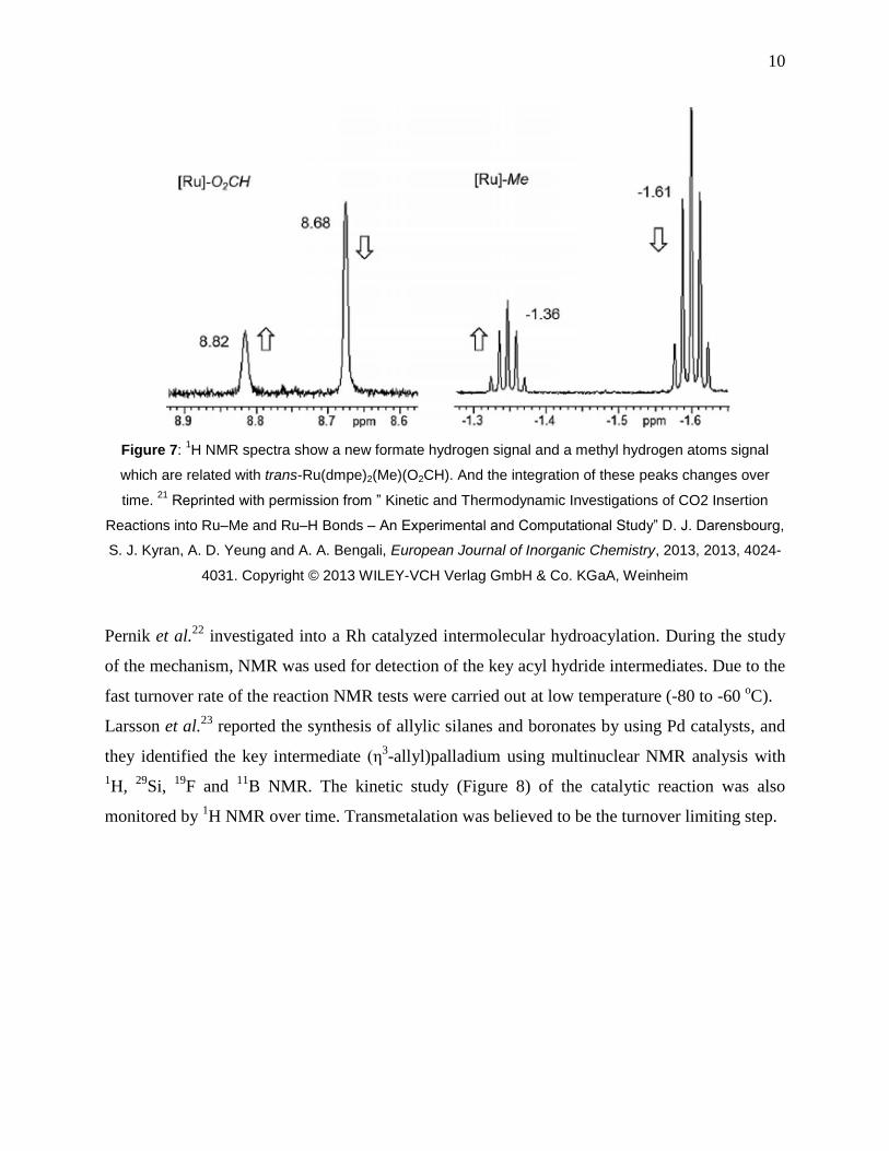
Figure 7: 1H NMR spectra show a new formate hydrogen signal and a methyl hydrogen atoms
signal which are related with trans-Ru(dmpe)2(Me)(O2CH). And the integration of these peaks
changes over time. 21
Reprinted with permission from ” Kinetic and Thermodynamic
Investigations of CO2 Insertion Reactions into Ru–Me and Ru–H Bonds – An Experimental and
Computational Study” D. J. Darensbourg, S. J. Kyran, A. D. Yeung and A. A. Bengali, European
Journal of Inorganic Chemistry, 2013, 2013, 4024-4031. Copyright © 2013 WILEY-VCH
Verlag GmbH & Co. KGaA, Weinheim ....................................................................................... 10
Figure 8: Synthesis of allylic silanes and boronates by using Pd catalysts reaction was monitored
by 1H NMR over 12 hours. Different species were tracked.
23 The concentration of each species
correspond to the NMR signal integration. Reprinted with permission from “Mechanistic
Investigation of the Palladium-Catalyzed Synthesis of Allylic Silanes and Boronates from Allylic
Alcohols” J. M. Larsson and K. J. Szabó, Journal of the American Chemical Society, 2012, 135,
443-455. Copyright © 2012 American Chemical Society ............................................................ 11
Figure 9: Generation of the solvate complex [Rh(Me-DuPHOS)(MeOH)2]BF4. cod=
cyclooctadiene; coe = cyclooctene25
............................................................................................ 12
Figure 10: Reaction data for the stoichiometric hydrogenation of 0.01 mmol [Rh(Me-
DuPHOS)(cod)]BF4 in 15 mL MeOH at 25 oC and 1 bar overall pressure (cycle time 3 min, layer
thickness 0.5 cm).25
Reprinted with permission from “Kinetic and mechanistic investigations in
homogeneous catalysis using operando UV/vis spectroscopy” C. Fischer, T. Beweries, A. Preetz,
H.-J. Drexler, W. Baumann, S. Peitz, U. Rosenthal and D. Heller, Catalysis Today, 2010, 155,
282-288. Copyright © 2009 Elsevier B.V. ................................................................................... 12
Figure 11: Extinction diagram (left) and comparison of spectroscopic values (points) and values
fitted as pseudo-first order (solid line) for several wavelengths.25
Reprinted with permission from
x
“Kinetic and mechanistic investigations in homogeneous catalysis using operando UV/vis
spectroscopy” C. Fischer, T. Beweries, A. Preetz, H.-J. Drexler, W. Baumann, S. Peitz, U.
Rosenthal and D. Heller, Catalysis Today, 2010, 155, 282-288. Copyright © 2009 Elsevier B.V.
....................................................................................................................................................... 12
Figure 12: Attenuated Total Reflectance (ATR). ......................................................................... 14
Figure 13: Latest version of React-IR, the ReactIR™ 45m.36
...................................................... 14
Figure 14: ReactIR spectrum of lithiation of N-Boc pyrrolidine compound.37
Reprinted with
permission from “Enantioselective, Palladium-Catalyzed α-Arylation of N-Boc Pyrrolidine: In
Situ React IR Spectroscopic Monitoring, Scope, and Synthetic Applications” G. Barker, J. L.
McGrath, A. Klapars, D. Stead, G. Zhou, K. R. Campos and P. O’Brien, The Journal of Organic
Chemistry, 2011, 76, 5936-5953. Copyright © 2011 American Chemical Society ..................... 15
Figure 15: Overlay of different spectra including starting reagents, product and putative imine
intermediate.38
Reprinted with permission from “Mannich-like three-component synthesis of α-
branched amines involving organozinc compounds: ReactIR monitoring and mechanistic
aspects” E. Le Gall, S. Sengmany, C. Hauréna, E. Léonel and T. Martens, Journal of
Organometallic Chemistry, 2013, 736, 27-35. Copyright © 2013 Elsevier B.V. ........................ 16
Figure 16: MALDI (left) and ESI sources.41, 42
Reprinted with permission from “Electrospray
and MALDI Mass Spectrometry: Fundamentals, Instrumentation, Practicalities, and Biological
Applications, Second Edition” R. B. Cole, Electrospray and MALDI Mass Spectrometry:
Fundamentals, Instrumentation, Practicalities, and Biological Applications, John Wiley & Sons,
2009. Copyright © 2010 John Wiley & Sons, Inc. ....................................................................... 17
Figure 17: ESI-MS study of the mechanism of a Baylis-Hillman reaction catalyzed by
DABCO.58
..................................................................................................................................... 18
Figure 18: Charged intermediates were detected during the DKR of amines reaction, each
intermediate can be represented by a characteristic peak.60
Reprinted with permission from
“Shvo's catalyst in chemoenzymatic dynamic kinetic resolution of amines – inner or outer sphere
mechanism?” B. G. Vaz, C. D. F. Milagre, M. N. Eberlin and H. M. S. Milagre, Organic &
Biomolecular Chemistry, 2013, 11, 6695-6698. Copyright © The Royal Society of Chemistry
2013............................................................................................................................................... 19
Figure 19: Shvo’s catalyst catalysed amine racemization mechanism revealed by ESI-MS.60
Reprinted with permission from “Shvo's catalyst in chemoenzymatic dynamic kinetic resolution
of amines – inner or outer sphere mechanism?” B. G. Vaz, C. D. F. Milagre, M. N. Eberlin and
H. M. S. Milagre, Organic & Biomolecular Chemistry, 2013, 11, 6695-6698. Copyright © The
Royal Society of Chemistry 2013 ................................................................................................. 20
Figure 20: Collision-induced fragmentation of cationic species.61
Reprinted with permission
from “C–H Activation at a Ruthenium(II) Complex – The Key Step for a Base-Free Catalytic
Transfer Hydrogenation?” L. Taghizadeh Ghoochany, C. Kerner, S. Farsadpour, F. Menges, Y.
Sun, G. Niedner-Schatteburg and W. R. Thiel, European Journal of Inorganic Chemistry, 2013,
2013, 4305-4317. Copyright © 2013 WILEY-VCH Verlag GmbH & Co. KGaA, Weinheim .... 21
Figure 21: ESI-MS of dba-free arylpalladium species.62
Reprinted with permission from ““Dba-
free” palladium intermediates of the Heck–Matsuda reaction. A. H. L. Machado, H. M. S.
Milagre, L. S. Eberlin, A. A. Sabino, C. R. D. Correia and M. N. Eberlin, Organic &
Biomolecular Chemistry, 2013, 11, 3277-3281. Copyright © The Royal Society of Chemistry . 22
Figure 22: MS/MS of MAO anion m/z 1881.63
Ten losses of 72 Da from the parent ion are
indicated by red arrows with a second series of fragment ions occurring at −16 Da, between m/z
1075 and 1507, depicted by blue arrows.Reprinted with permission from “Mass Spectrometric

xi
Characterization of Methylaluminoxane” T. K. Trefz, M. A. Henderson, M. Y. Wang, S. Collins
and J. S. McIndoe, Organometallics, 2013, 32, 3149-3152. Copyright © 2013 American
Chemical Society .......................................................................................................................... 23
Figure 23: CID (collision induced dissociation) mass spectrum of the ion at m/z=1000.3, a Rh(I)
intermediate.64
Reprinted with permission from “Direct Detection of Key Intermediates in
Rhodium(I)-Catalyzed [2+2+2] Cycloadditions of Alkynes by ESI-MS” M. Parera, A. Dachs, M.
Solà, A. Pla-Quintana and A. Roglans, Chemistry – A European Journal, 2012, 18, 13097-
13107. Copyright © 2012 WILEY-VCH Verlag GmbH & Co. KGaA, Weinheim ..................... 24
Figure 24: The desolvation process in electrospray ionization. Modified with permission of the
author from Henderson, W., McIndoe J. S., Mass Spectrometry of Inorganic and Organometallic
Compounds. John Wiley & Sons, Ltd. West Sussex: 2005, p. 92. ............................................... 27
Figure 25: (a) IEM: Small ion ejection from a charged nanodroplet. (b) CRM: Release of a
globular protein into the gas phase.86
Reprinted with permission from “Unraveling the
Mechanism of Electrospray Ionization” L. Konermann, E. Ahadi, A. D. Rodriguez and S.
Vahidi, Analytical Chemistry, 2012, 85, 2-9. Copyright © 2012 American Chemical Society ... 28
Figure 26: Electrospray source with QTOF-Micro scheme.87
Reprinted with permission from
“Micromass Q-TOF micro Mass Spectrometer Operator’s Guide” Copyright © 2012 Waters
Corporation ................................................................................................................................... 29
Figure 27: The Ion Optical System of the Q-TOF micro.87
Reprinted with permission from
“Micromass Q-TOF micro Mass Spectrometer Operator’s Guide” Copyright © 2012 Waters
Corporation ................................................................................................................................... 30
Figure 28: The Prefilter and Main Analyzer of the Q-TOF micro87
Reprinted with permission
from “Micromass Q-TOF micro Mass Spectrometer Operator’s Guide” Copyright © 2012
Waters Corporation ....................................................................................................................... 31
Figure 29 Positive-ion energy-dependent ESI-MS of a representative example.X axis is the m/z,
Y axis is collision energy in voltage, the red and blue dots are the detected signal of a certain
species at the applied voltage.88
Reprinted with permission from “Synthesis and characterization
of a new class of anti-angiogenic agents based on ruthenium clusters” A. A. Nazarov, M. Baquié,
P. Nowak-Sliwinska, O. Zava, J. R. van Beijnum, M. Groessl, D. M. Chisholm, Z. Ahmadi, J. S.
McIndoe, A. W. Griffioen, H. van den Bergh and P. J. Dyson, Sci. Rep., 2013, 3. Copyright ©
2013 Macmillan Publishers Limited ............................................................................................. 32
Figure 30 Time of Flight analyzer87
Reprinted with permission from “Micromass Q-TOF micro
Mass Spectrometer Operator’s Guide” Copyright © 2012 Waters Corporation .......................... 33
Figure 31 Pressurized sample infusion system setup. ................................................................... 35
Figure 32: Normalized intensity vs. time trace for a charged silane (m/z 349) and appearance of
the product of redistribution (m/z 425).72
...................................................................................... 36
Figure 33: Proposed mechanism for hydrogenation of alkyne by Wilkinson’s catalyst.95
........... 37
Figure 34: Powersim Numerical model95
, this figure represents a Wilkinson’s hydrogenation
reaction. ......................................................................................................................................... 38
Figure 35: COPASI interface ........................................................................................................ 39
Figure 36: COPASI model for reversible reaction ....................................................................... 40
Figure 37: simulation method of COPASI.................................................................................... 41
Figure 38: Powersim model for irreversible first order reaction. ................................................. 41
Figure 39: Reductive elimination.................................................................................................. 42
Figure 40: Dimer splits into two monomers ................................................................................. 43
Figure 41: Oxidative addition ....................................................................................................... 44
xii
Figure 42: Reversible reductive elimination ................................................................................. 45
Figure 43: Powersim model for second order reversible reaction. ............................................... 46
Figure 44: Glovebox next to MS .................................................................................................. 47
Figure 45: Online monitoring with blocked PEEK tubing ........................................................... 48
Figure 46: Eight generations of filter ............................................................................................ 49
Figure 47: The new online dilution system................................................................................... 51
Figure 48: Photo of online dilution system. .................................................................................. 51
Figure 49: PSI NMR tube ............................................................................................................. 52
Figure 50: PSI sample vial. In a glovebox, small amounts of solid sample can be introduced into
a vial capped with a septum, then taken out of the glovebox and solvent injected into it. Two
PEEK tubes pierce through a septum into the vial. The yellow PEEK tube is connected to a
pressure supply (e.g. Ar or N2), and the red PEEK tube is dipped into the solution and the other
end is connected to the ESI-MS. If the sample is not soluble enough, a filter must be installed on
the red PEEK tube and the septum fitted before the vial is capped. ............................................. 53
Figure 51: Energetics of the PK reaction. Reprinted with permission from “Density Functional
Studies on the Pauson−Khand Reaction” M. Yamanaka and E. Nakamura, Journal of the
American Chemical Society, 2001, 123, 1703-1708. Copyright © 2001 American Chemical
Society........................................................................................................................................... 56
Figure 52: Functionalized pyrrolidinium and piperidinium salts. X– = Br
–, PF6
–, BPh4
–, Tf2N
–. . 59
Figure 53: Positive-ion ESI-MS in dichloromethane [Co2(CO)6(4-3)][PF6] (top) and
[Co2(CO)6(4-1)][PF6] (bottom). In both cases, the single peak corresponds to the intact cation. 61
Figure 54: Single crystal X-ray structure of the cationic part of [Co2(CO)6(4-1)]+ [BPh4]
–. The
tetraphenylborate anion is not shown for the sake of clarity. Key bond lengths: Co1-Co2 2.461
Å; C7-C8 1.334 Å; C8-C9 1.488 Å; 1.311 0.01 Å; Co-C 1.96 0.01 Å; C-O 1.13 0.01 Å; Co-
CO 1.81 0.02 Å; C-N 1.52 0.02 Å. Key bond angles: C6-C7-C8 146.2°; Co-Co-C 51 1°,
Co-C-Co 77.5 0.3°. .................................................................................................................... 62
Figure 55: Gas phase reactions of [Co2(CO)6(4-1)]+ with three different alkenes at a cone voltage
of 20 V. In each case, one CO ligand is removed and the alkene adds to [Co2(CO)5(1)]+. The
alkene does not add to the fully saturated ion. .............................................................................. 62
Figure 56: Abundance vs. time data for [4-3]+ (starting material), [Co2(CO)6(4-3)]
+
(intermediate) and [4-3 + CO]+ (product). Data collected using positive ion PSI-ESI-MS in
chlorobenzene, online dilution with acetone, Schlenk flask saturated and pressurized with CO.
Data has been normalized to the total ion current. Scan time of 10 seconds per spectrum.
Approximately 20% of the total ion current at the end of the reaction consisted of numerous low
abundance by-products, none of which exceeded 5% of the total. ............................................... 65
Figure 57: During the PSI-ESI-MS, the collision voltage was set to 2 V. The breakdown graph
shows [Co2(CO)6(4-3)]+ is a stable species at this voltage and it can only be fragmented when the
collision voltage reaches 8 V. ....................................................................................................... 66
Figure 58: Intensity vs. time data for [Co2(CO)6(4-3)]+ (starting material) and [4-3 + CO]
+
(product), collected at three different temperatures. Inset: Eyring plot for the three different
temperatures. ................................................................................................................................. 67
Figure 59: Positive ions of ionized Wilkinson’s catalyst, where 5-1+ is [Ph2P(CH2)4PPh2Bn]
+.
Reprinted with permission from “Mono-alkylated bisphosphines as dopants for ESI-MS analysis
of catalytic reactions” D. M. Chisholm, A. G. Oliver and J. S. McIndoe, Dalton Transactions,
2010, 39, 364-373. Copyright © 2010 Royal Society of Chemistry ............................................ 79
xiii
Figure 60: X-ray crystal structure of [Ph3P(CH2)4C2H]+ I
–. Key structural parameters: C5-C6
1.118 A; C4-C5-C6 177.51°. ........................................................................................................ 82
Figure 61:. X-ray crystal structure of [Ph3P(CH2)4C2H]+ I
– (the precursor to 5-4). Key structural
parameters: C5-C6 1.118 A; C4-C5-C6 177.51°. ......................................................................... 84
Figure 62: Positive-ion ESI-MS in fluorobenzene, [PPh3P(CH2)4CCH]PF6 (bottom) is the starting
material. [PPh3P(CH2)5CH3]PF6 (top) is the final product. ........................................................... 86
Figure 63 Relative intensity vs time traces for alkyne (5-4), alkene (5-5) and alkane (5-6). ....... 86
Figure 64: Traces for disappearance of alkyne (top), appearance and disappearance of alkene
(middle), and appearance of alkane (bottom) at temperatures of 0°C, 23°C and 58°C. ............... 88
Figure 65: Catalytic cycle for hydrogenation of alkyne to alkane, where the two hydrogenations
compete with one another. ............................................................................................................ 89
Figure 66: Match between simulated and experimental reaction progress curves. The thin black
lines are the experimental curves; the thick transparent lines are the calculated curves. ............. 90
Figure 67: Experimental traces for hydrogenation of 5-4 using Wilkinson’s catalyst (5 mol%) at
91°C in the presence of (a) no added PPh3, (b) one equivalent of PPh3, and (c) two equivalents of
PPh3. The right-hand column shows the corresponding traces calculated by the numerical model,
wherein only the starting concentration of PPh3 has been altered. ............................................... 92
Figure 68: Alkane hydrogenation product. Key bond lengths and angles: C5-C6 1.500 A; C4-C5-
C6 113.83°. ................................................................................................................................... 95
Figure 69: Hydrogenation of [Ph3P(CH2)4CH=CH2][PF6] under 3 psi of H2, with 13.3% of
[Rh(PR3)2(FPh)]+[BAr
F4]
– as catalyst at room temperature with FPh as solvent. Inset: relative
intensity vs time plot exhibiting behavior of [Rh(PR3)2(FPh)]+ (5-7) and [Rh(PR3)2]
+ (5-8). ..... 96
Figure 70: Top: disappearance of alkyne 5-4 at 0, 23, 38 and 49°C (fast at all temperatures).
Middle: appearance and consumption of alkene 3. Bottom: appearance of alkane 5-6. .............. 97
Figure 71: Reaction rate as a function of catalyst loading, illustrating that the reaction is first
order in the concentration of [RhP2(FPh)]+[BAr
F4]
– used. ........................................................... 98
Figure 72: Selective hydrogenation of the charge-tagged alkyne in the presence of 1.1
equivalents of H2. Inset: ln[x] vs time plot exhibiting 1st order behavior. ................................... 98
Figure 73: Comparison of hydrogenation with excess hydrogen and one equivalent of hydrogen.
....................................................................................................................................................... 99
Figure 74: Reaction profiles for the reduction of alkyne to alkane using H2 (blue/yellow) vs. D2
(green/red). .................................................................................................................................... 99
Figure 75: Precatalyst signal before hydrogenation started: mostly [RhP2(PhF)]+. ................... 100
Figure 76: Precatalyst signal after hydrogenation started: a mix of [RhP2]+ and [RhP2(PhF)]
+. 101
Figure 77: Mass spectrum of [Rh(PR3)2(octyne)n]+ (n = 1, left, and n = 2, right). Experimental
data shown by line, calculated isotope pattern shown by columns............................................. 101
Figure 78: Pathways for alkene hydrogenation, after Schrock and Osborn. .............................. 102
Figure 79: The effect of NEt3 on the rate and selectivity of hydrogenation. .............................. 103
Figure 80: Addition of NEt3 leads to the disappearance of [RhP2]+ and the appearance of
[HNEt3]+. ..................................................................................................................................... 104
Figure 81: The mechanism of alkyne/alkene hydrogenation. P = P(cyclopropyl)3. ................... 105
Figure 82: Direct comparison between simulated (coloured lines) and experimental results
(black). The simulation is for the genetic algorithm, but similarly good matches were obtained
for the other methods. ................................................................................................................. 107
Figure 83: Competition reaction: reduction of alkyne vs. alkene. Note that the alkenes remain
essentially untouched until the alkyne is completely consumed. Reduction of the two alkenes

xiv
proceed at similar pace, though the hydrogenation of [Ph3P(CH2)3CH=CH2]+ was slightly faster
than that of [Ph3P(CH2)4CH=CH2]+. ........................................................................................... 108
Figure 84: Dehydrocoupling of silanes for early transition metal complexes, following the σ
bond metathesis mechanism. ...................................................................................................... 114
Figure 85: Dehydrocoupling of silanes for late transition metal complexes, following the
oxidative addition/reductive elimination mechanism. ................................................................ 115
Figure 86: 1,2 silyl migration (or silylene insertion) mechanism for dehydrocoupling of silanes
by late transition metal complexes. ............................................................................................. 115
Figure 87: Proposed dehydrocoupling of silane mechanism based on observation. .................. 116
Figure 88: Charged phosphine ligand benzyl(4-(diphenylphosphino)butyl)diphenylphosphonium
hexafluorophosphate(V). ............................................................................................................ 117
Figure 89: Red species should be visible in ESI-MS by using a charged silane substrate. ........ 117
Figure 90: Hydrolysis of diclorosilane ....................................................................................... 118
Figure 91: Hydrolysis and condensation of hydrosilanes. .......................................................... 118
Figure 92: Cationic oxorhenium catalyst for hydrolysis of silane. ............................................. 119
Figure 93: A ruthenium complex catalyzed hydrolysis of silane mechanism proposed by Lee et
al.215
............................................................................................................................................. 119
Figure 94: Fe complex for hydrosilation .................................................................................... 120
Figure 95: The Chalk-Harrod mechanism. ................................................................................. 121
Figure 96: Proposed Ru–silylene-based catalytic cycle.............................................................. 122
Figure 97: X-ray crystal structure of compound 6-5. ................................................................. 123
Figure 98: Dehydrocoupling of silanes catalyzed by Wilkinson’s catalyst, RhCl(PPh3)3. ......... 124
Figure 99: Hydrolysis of silanes catalyzed by Wilkinson’s catalyst, RhCl(PPh3)3. ................... 124
Figure 100: PSI-ESI-MS online monitoring result of hydrolysis of silane. Left: whole reaction
process over 130 minutes. Reaction started when RhCl(PPh3)3 was introduced into reaction
system around the 8th minute. Right: enlarged graph of converting part. The whole reaction
finished in 3 minutes. .................................................................................................................. 125
Figure 101: PSI-ESI-MS online monitoring result of hydrolysis of silane. Whole reaction process
was over 210 minutes. Reaction started when RhCl(PPh3)3 was introduced into reaction system
around the 10th minute. .............................................................................................................. 126
Figure 102: Hydrolysis of silanes, even longer oligomer products were detected. .................... 127
Figure 103: PSI-ESI-MS online monitor of hydrolysis of silane by [Cp*Ru(MeCN)3][PF6]. The
data quality is poor because the PEEK tubing was partially blocked by large molecular weight
oligomer products. Target product %P485 is stable with water, no hydrolysis of silane. .......... 128
Figure 104: Silane alcoholysis between 6.5 and MeOH under 51 oC. ........................................ 129
Figure 105: Silane alcoholysis between 6-5 and MeOD under 51 oC. ....................................... 130
Figure 106: Relative intensity vs time for Wilkinson’s catalyst fragment [Rh(PPh3)3]+ at
m/z=889.7. .................................................................................................................................. 131
Figure 107: A potential intermediate of alcoholysis of silane by Wilkinson’s catalyst. ............ 131
Figure 108: Mixture of potential intermediates, mixture of two potential intermediate with
formular [(PPh3)2RhCl+MeSi(CH2)3PPh3+H]+ (blue peaks) and
[(PPh3)2RhCl+MeSi(CH2)3PPh3+D]+(gray peaks) at ratio 1:2. .................................................. 132
Figure 109: CdSe-DHLA for H2 production. .............................................................................. 136
Figure 110: Difference between adding and not adding Ni in the hydrogen production system.
..................................................................................................................................................... 136
Figure 111: FeS cluster samples ................................................................................................. 138
xv
Figure 112: MS of the Fe4S4(Cy3)4 cluster, the blue bar is the calculated isotope pattern, the line
is the experimental data. ............................................................................................................. 138
Figure 113: MS/MS of the 7.2-1. We can see many fragments of the mother ion-1472.9, the
daughter ions: 1192.6, 912.0, 631.9 and 351.7 are due to lose of PCy3. .................................... 139
Figure 114: MS/MS of the 7.2-2, 623.7 is [7.2-2 + Et4N]+, 493.5 is 7.2-2, 458.5 is [7.2-2 – Cl]
+.
..................................................................................................................................................... 139
Figure 115: MS/MS of 7.2-3, 838.0 is [7.2-2 + Et4N]+, 618.8 is [7.2-2 - SBu]
+, 383.6 is [7.2-2 –
3*SBu]+ ....................................................................................................................................... 140
Figure 116: Structure of the cationic zinc complex. ................................................................... 141
Figure 117: MS data of the Zn complex and the calculated isotope pattern (blue bars). ........... 141
Figure 118: MS of intermediate in copper-mediated fluorination Reprinted with permission from
“Copper-Mediated Fluorination of Arylboronate Esters. Identification of a Copper(III) Fluoride
Complex” P. S. Fier, J. Luo and J. F. Hartwig, Journal of the American Chemical Society, 2013,
135, 2552-2559. Copyright © 2013 American Chemical Society .............................................. 143
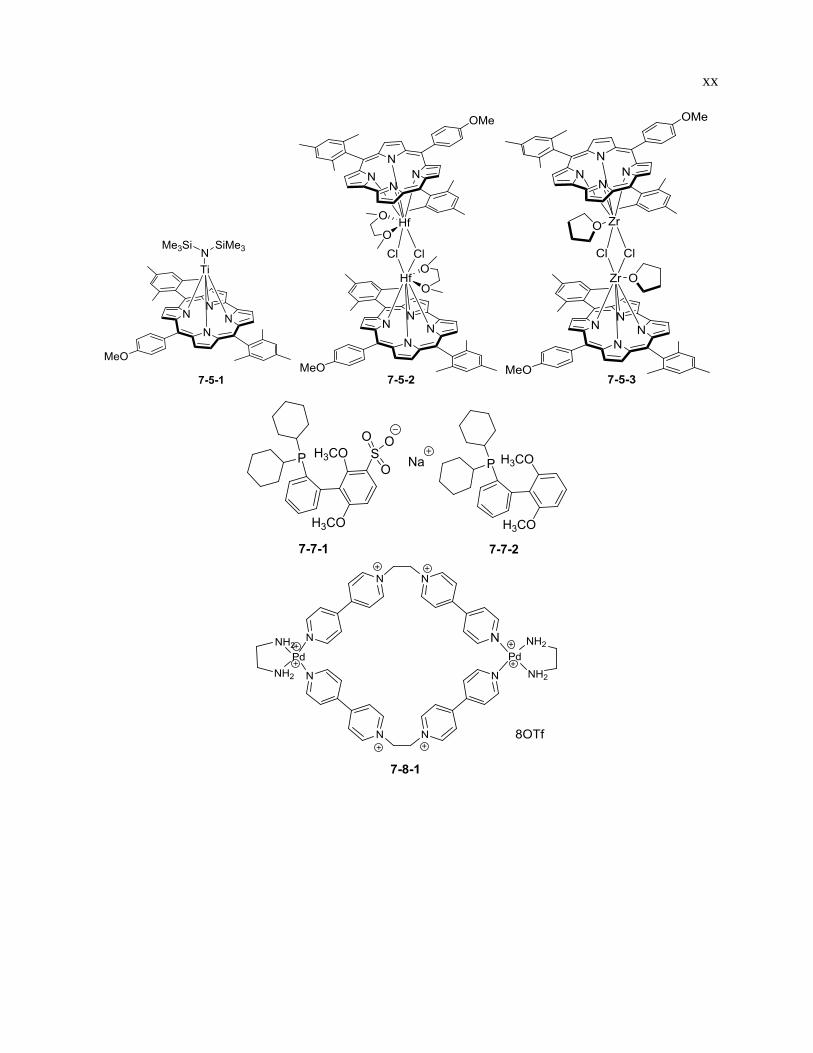
Figure 119: Ti, Hf and Zr complexes.......................................................................................... 144
Figure 120: MS experimental data shows as [M+Na-H]+ of 7-5-1, calculated isotope pattern of
[M+Na-H]+ .................................................................................................................................. 145
Figure 121: Ligands for Pd(η3-1-PhC3H4)(η
5-C5H5) activation. ................................................. 146
Figure 122: Negative mode, ESI-MS. Addition of Pd(η3-1-Ph-C3H4)(η
5-C5H5) to charged ligand
7-7-1 makes ligand disappear over the course of about 20 minutes. .......................................... 147
Figure 123: (7.7.1)2Pd species is the main Pd containing peak in the reaction, however the
calculated isotope pattern (blue bars) shows a extra H is present. .............................................. 147
Figure 124: In positive mode of ESI-MS. Reaction with 7-7-2 as ligand. The blue species is
[PhC3H4+7.7.2]+, the red species is [η
3-1-PhC3H4+Pd+7-7-2]
+ ................................................. 148
Figure 125: Proposed mechanism for hydroacylation by rhodium complexes........................... 149
Figure 126: Hydroacylation catalytic cycle with reaction online monitoring results. ................ 151
Figure 127: Weak bonding supramolecular complexes characterized by CSI. .......................... 153
Figure 128: Experiment data of 7-8-1 (2+) and calculated isotope pattern (blue bars) .............. 153
Figure 129: Experimental data of 7-8-2 (4+) and calculated isotope pattern (blue bars) ........... 154
xvi
List of Abbreviations
[X]– anion
[X]+ cation
Ar aryl
b.p
Boc
boiling point
tert-Butyl carbamates
bpy tbucope
2,2’-bipyridyl
(C8H14)PC6H4CH2P(tBu)2
cat catalyst
CI chemical ionization
CID collision induced dissociation
COD cyclooctadiene
Col V collision voltage
CSI CryoSpray Ionization
Cp cyclopentadienyl ligand
Cp* pentamethylcyclopentadienyl ligand
CV cone voltage
Da DABCO
Dalton
1,4-diazabicyclo[2.2.2]octane
DFT
DHLA
dppp
density functional theory
Dihydrolipoic acid
1,3-Bis(diphenylphosphino)propane
EDESI energy-dependent electrospray ionization
EDG electron donating group
EI electron impact
EPR electron paramagnetic resonance
ESI electrospray ionization
ESI(-)-MS negative-ion electrospray ionization mass
spectrometry
ESI(+)-MS positive-ion electrospray ionization mass
spectrometry
FT-ICR Fourier transform ion cyclotron
resonance
GC gas chromatography
GPC
Hex
gel permeation chromatography
hexyl group
HPLC high performance liquid chromatography
ID inner diameter
iPr isopropyl
IR infrared
IS internal standard
KE kinetic energy
KIE kinetic isotope effect
L ligand
xvii
m meta
m.p. melting point
m/z mass-to-charge ratio
MALDI matrix-assisted laser desorption
ionization
MAO methylaluminoxane
MCP microchannel plate
Me methyl
MS mass spectrometry/ mass spectrometer/
mass spectrum
MS/MS tandem mass spectrometry
NMR nuclear magnetic resonance
OA oxidative addition
OAc acetate
OTf trifluoromethanesulfonate
p
PcPr3
PCy3
para
tricyclopropylphosphane
Tricyclohexylphosphine
PEEK polyetheretherketone
[PF6]– hexafluorophosphate
Ph phenyl
ppm parts per million
PSI pressurized sample infusion
Q-TOF quadrupole-time-of-flight
RE reductive elimination
RF radio frequency
RSD
SBu
relative standard deviation
-S-[(CH2]3CH3]
SPS Solvent Purification System
tBu tertiary butyl
THF tetrahydrofuran
TIC total ion current
TOF time-of-flight
UV ultraviolet
UV/Vis ultraviolet/visible

xviii
List of Structures

xix
xx
xxi

xxii
Acknowledgments
Firstly I would like to thank my supervisor Professor Scott McIndoe for his teaching, supporting,
encouraging and inspiring in my five years’ Ph.D study. My thanks to him for teaching me how
to manage my time instead of hurrying me up when I was slow on research. I feel so lucky to be
in such a great research team.
Thank you to all past and present members of the McIndoe group (Ali, Matt, Danielle, Mike,
Jenny, Tyler, Krista, Cara, Miles, Jessamyn, Lars, Eric, Rhonda and Zohrab) and my fellow past
and present graduate students across the department of University of Victoria and University of
Montreal, for sharing your help and great stories to make every day enjoyable. Especial thanks to
Dr. Zohrab Ahmadi for working together with me and sharing knowledge and experience with
me for four years, and Rhonda Stoddard for helping me and understand me. Especial thanks to
Peter Lee as a labmate and roommate who shared his chemistry knowledge, optimistic attitude
and same house with me for two and half years..
I also really appreciate Professor Lisa Rosenberg and Professor Garry Hanan for their help on
my research. I want to thank UVic faculty and staff for all their technical support and expertise. I
am also most grateful to Dr. Ori Granot for helping me with all MS instrument issues, Dr. Allen
Oliver for providing the X-ray crystallography and Christopher Barr for NMR services.
The bottom of this appreciation letter is also from the bottom of my heart, I will never make
these achievements without the love and selfless support of my mom Xiaohua Wang and my dad
Shimin Luo. They are great parents who sacrifice their life to raise me and support me, whenever
I fall down; they help me to stand up. They both did not have a chance to go to university, but
they deserve to have their name printed in a doctor’s thesis. I love you forever.

xxiii
Dedication
To Mom and Dad

1
1. Literature Review
1.1 Organometallic catalysis
Synthetic chemicals are an essential part of our daily life. Countless chemicals are synthesized
efficiently by optimising the production process to reduce reaction time, waste and expense. This
cannot happen without catalysis. The function of a catalyst is to make the reaction faster and/or
more selective for the target molecule, and theoretically catalysts can be recycled 100 percent as
they are not consumed in the reaction. Ideally, they allow atom-economical reactions (which
avoid protecting groups and minimize waste). Traditional stoichiometric strategies are gradually
being replaced by this new “greener” chemistry and this is an inevitable trend for the future of
chemistry.1
Catalysts do not appear in the overall reaction equation nor do they influence the
thermodynamics of a reaction, however they change the reaction pathway and lower the
activation energy, and can also boost the selectivity of one product over another (especially
important in enantioselective reactions). Organometallic catalysis involves the activation of
organic molecules and their transformation by metals from the main group, transition metals,
lanthanides and actinides.2, 3
Transition metal catalysts especially have been applied in many
industrial applications due to their ability to achieve sufficient yields of pure target products, in
which some of these products cannot be synthesized without using catalysts (e.g. olefin
metathesis, crosscoupling, hydrogen fuel cells). One of the major differences between transition
metal and main group elements is the presence of d electrons in the valence shell.4 This property
gives transition metals great potential for catalytic reactions: (1) the transition metal can have
different coordination numbers, so the binding geometry is variable; (2) they can easily gain or
lose electrons in redox processes, during which their oxidation state will also change
accordingly; (3) transition metals can form both σ bonds and π bonds with other molecules; (4)
transition metals can form chemical bonds with a variety of different ligands, and the presence of
ligands can help the metal with steric targeting and can influence the electron distribution at the
metal center.5

2
Catalysts can also be classified as homogeneous and heterogeneous based on their physical state.
Most industrial catalysts are heterogeneous (i.e. they are in the solid state whereas the reactants
are in the gas or sometimes solution phase), but in this thesis, we mainly focus on homogeneous
catalysis reactions (in which all components are in solution). Homogeneous reactions are
inherently easier to study, and the mechanistic insights so gained are often transferable to
heterogeneous systems.
Some notable examples of modern organometallic chemistry are contained in the 2005 and 2010
Nobel Prizes in Chemistry. In 2005, Yves Chauvin, Robert H. Grubbs and Richard R. Schrock
won the prize “for the development of the metathesis method in organic synthesis”.6
Equation 1: Metathesis of alkenes
However, catalyzed metathesis was discovered a long time before the catalyst’s role in the
reaction was understood. In 1970, Yves Chauvin published a paper proposing the catalyst is a
metal alkylidene, and later he used experimental results to explain the mechanism,7 and now this
mechanism is well accepted.
Scheme 1: Chauvin’s mechanism for alkene metathesis

3
Grubbs and Schrock did a lot of the mechanistic work proving Chauvin’s theory, especially
Grubbs. They developed independent and highly complementary catalytic systems, and
nowadays, they are extremely useful in the synthesis of pharmaceuticals, agrochemicals,
materials etc.8 Grubbs’ catalysts are based on ruthenium whereas Schrock’s on molybdenum
(Figure 1).
Figure 1: (1) First asymmetric Schrock catalyst; (2) 1st Generation Grubbs' Catalyst; (3) 2nd Generation
Grubbs' Catalyst
In 2010, Richard F. Heck, Ei-ichi Negishi and Akira Suzuki won the Nobel prize for “palladium-
catalyzed cross couplings in organic synthesis”. These catalysts are efficient for activating
various organic compounds and catalyzing the formation of new carbon-carbon bonds, and have
become an essential methodology for total synthesis of new drugs and materials.9
The Heck reaction is between an organohalide compound and an alkene to form a substituted
alkene (Figure 2).10-12
Figure 2: Catalytic cycle for Heck reaction
4
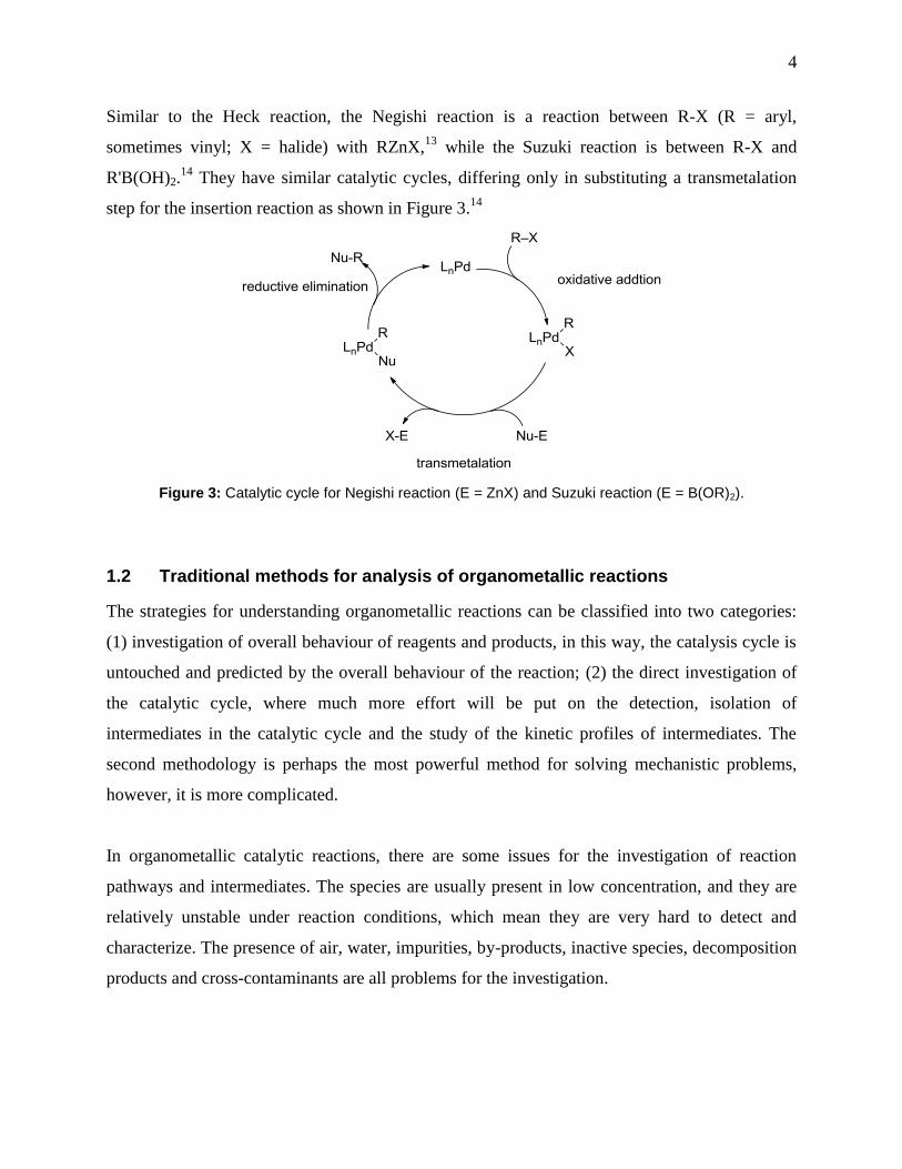
Similar to the Heck reaction, the Negishi reaction is a reaction between R-X (R = aryl,
sometimes vinyl; X = halide) with RZnX,13
while the Suzuki reaction is between R-X and
R'B(OH)2.14
They have similar catalytic cycles, differing only in substituting a transmetalation
step for the insertion reaction as shown in Figure 3.14
Figure 3: Catalytic cycle for Negishi reaction (E = ZnX) and Suzuki reaction (E = B(OR)2).
1.2 Traditional methods for analysis of organometallic reactions
The strategies for understanding organometallic reactions can be classified into two categories:
(1) investigation of overall behaviour of reagents and products, in this way, the catalysis cycle is
untouched and predicted by the overall behaviour of the reaction; (2) the direct investigation of
the catalytic cycle, where much more effort will be put on the detection, isolation of
intermediates in the catalytic cycle and the study of the kinetic profiles of intermediates. The
second methodology is perhaps the most powerful method for solving mechanistic problems,
however, it is more complicated.
In organometallic catalytic reactions, there are some issues for the investigation of reaction
pathways and intermediates. The species are usually present in low concentration, and they are
relatively unstable under reaction conditions, which mean they are very hard to detect and
characterize. The presence of air, water, impurities, by-products, inactive species, decomposition
products and cross-contaminants are all problems for the investigation.
5
With these issues in mind, and considering current techniques and methodologies, this chapter
will discuss some of the many techniques that are currently used in this research field.
1.2.1 NMR Spectroscopy
Nuclear magnetic resonance (NMR) spectroscopy provides detailed information about the
physical and chemical properties of molecules.15
It is the most important method for the
structural determination of molecules. Based on coupling constants, chemical shift, relaxation
times, exchange lifetimes and intensities, the chemical environment of a certain atom (1H,
13C,
19F,
31P etc.) can be well explained. Furthermore, a variety of two dimensional and three
dimensional NMR experiments can provide data of through-bond and through-space interactions.
This is especially useful for metal elements in the organometallic compounds. For example, the
Rosenberg group investigated the mechanism of dehydrocoupling of silanes catalyzed by
Wilkinson’s catalyst. A number of NMR experiments were carried out, including 1H,
31P.
Different intermediates can be identified including the oxidative addition intermediate
Rh(PPh3)2(Cl)(H)(Si{nHex}2-H), hydrido complexes HRh(PPh3)3, H2Rh(PPh3)3Cl and
HRh(PR3)4.16
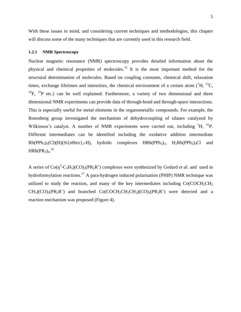
A series of Co(ƞ3-C3H5)(CO)2(PR2R’) complexes were synthesized by Godard et al. and used in
hydroformylation reactions.17
A para-hydrogen induced polarisation (PHIP) NMR technique was
utilized to study the reaction, and many of the key intermediates including Co(COCH2CH2
CH3)(CO)3(PR2R’) and branched Co(COCH2CH2CH3)(CO)3(PR2R’) were detected and a
reaction mechanism was proposed (Figure 4).

6
Figure 4: Para-hydrogen enhanced NMR is used to detect signals of H on different species in the
reaction, detected H is in red color.17
Reprinted with permission from “An NMR study of cobalt-catalyzed
hydroformylation using para-hydrogen induced polarisation” C. Godard, S. B. Duckett, S. Polas, R. Tooze
and A. C. Whitwood, Dalton Transactions, 2009, 2496-2509. Copyright © 2009 The Royal Society of
Chemistry

7
Multidimensional NMR is a powerful technique for characterizing chemical structures.
Zuccaccia et al. investigated the degradation process of two Ir oxidation catalysts,18
[Cp*Ir(H2O)3][NO3]2 (Cp* = pentamethylcyclopentadienyl) and [Cp*Ir(bzpy)(NO3)] (bzpy = 2-
benzoylpyridine). Their goal was to determine whether or not the degradation is initiated by
functionalization of Carbon atom (C-attack) or by hydrogen abstraction (H-attack) by using
NMR. Using a series of 2D 1H NMR experiments, the functionalization of the Cp* ligand could
be assigned (Figure 5). The two resulting intermediates where found to degrade via the C-attack
pathway.
Figure 5: 1H NOESY spectrum of oxidative degradation product of [Cp*Ir(bzpy)(NO3)]
18 Reprinted with
permission from “An NMR Study of the Oxidative Degradation of Cp*Ir Catalysts for Water Oxidation:
Evidence for a Preliminary Attack on the Quaternary Carbon Atom of the –C–CH3 Moiety” C. Zuccaccia,

8
G. Bellachioma, S. Bolaño, L. Rocchigiani, A. Savini and A. Macchioni, European Journal of Inorganic
Chemistry, 2012, 2012, 1462-1468. Copyright © 2012 Wiley-VCH Verlag GmbH & Co. KGaA, Weinheim
Mom et al. reported a series of ferrocenyl polyphosphane molecules,19
the structures of which
were studied by NMR and X-ray crystallography. 31
P NMR was heavily used in the research,
with coupling constants of interactions among long distance P atoms being used to give strong
support for the final confirmation of structures of these molecules in solution phase as shown in
Table 1.
Table 1: Ferrocenyl polyphosphanes structures and decoupled proton 31
P NMR data19
. Reprinted with
permission from “Congested Ferrocenyl Polyphosphanes Bearing Electron-Donating or Electron-
Withdrawing Phosphanyl Groups: Assessment of Metallocene Conformation from NMR Spin Couplings
and Use in Palladium-Catalyzed Chloroarenes Activation” S. Mom, M. Beaupérin, D. Roy, S. Royer, R.
Amardeil, H. Cattey, H. Doucet and J. C. Hierso, Inorganic Chemistry, 2011, 50, 11592-11603. Copyright
© 2011 American Chemical Society
Boutain et al.20
reported a parahydrogen based NMR study of an alkyne hydrogenation reaction
catalyzed by platinum(II) bis-phosphine triflate complexes. Key intermediates
[Pt(tbucope)(CHPhCH2Ph)][OTf] where
tbucope is (C8H14)PC6H4CH2P(tBu)2,
[Pt(dppp)(CHPhCH2Ph)][OTf] (where dppp is 1,3-Bis(diphenylphosphino)propane) and

9
[Pt(dppp)(CHPhCH-(OMe)Ph)][OTf] were observed based on a variety of 2D NMR experiments
including 1H-
31P (Figure 6) ,
1H-
195Pt,
1H-
13C as well as deuterium labelling reactions. A
hydrogenation mechanism was also proposed.
Figure 6: 1H-
31P HMQC spectrum indicates the existence of a key intermediate during the reaction.
20
Reprinted with permission from “A parahydrogen based NMR study of Pt catalysed alkyne hydrogenation”
M. Boutain, S. B. Duckett, J. P. Dunne, C. Godard, J. M. Hernandez, A. J. Holmes, I. G. Khazal and J.
Lopez-Serrano, Dalton Transactions, 2010, 39, 3495-3500. © The Royal Society of Chemistry 2010
Darensbourg et al.21
reported a kinetic study of a CO2 insertion reaction into Ru-Me and Ru-H
bonds of trans-Ru(dmpe)2(Me)H and trans-Ru(dmpe)2(Me)2 by 1H NMR (Figure 7) and IR
experiments. Their results showed that the insertion of CO2 into Ru-H required less activation
energy than into the Ru-Me bond.
10
Figure 7: 1H NMR spectra show a new formate hydrogen signal and a methyl hydrogen atoms signal
which are related with trans-Ru(dmpe)2(Me)(O2CH). And the integration of these peaks changes over
time. 21
Reprinted with permission from ” Kinetic and Thermodynamic Investigations of CO2 Insertion
Reactions into Ru–Me and Ru–H Bonds – An Experimental and Computational Study” D. J. Darensbourg,
S. J. Kyran, A. D. Yeung and A. A. Bengali, European Journal of Inorganic Chemistry, 2013, 2013, 4024-
4031. Copyright © 2013 WILEY-VCH Verlag GmbH & Co. KGaA, Weinheim
Pernik et al.22
investigated into a Rh catalyzed intermolecular hydroacylation. During the study
of the mechanism, NMR was used for detection of the key acyl hydride intermediates. Due to the
fast turnover rate of the reaction NMR tests were carried out at low temperature (-80 to -60 oC).
Larsson et al.23
reported the synthesis of allylic silanes and boronates by using Pd catalysts, and
they identified the key intermediate (η3-allyl)palladium using multinuclear NMR analysis with
1H,
29Si,
19F and
11B NMR. The kinetic study (Figure 8) of the catalytic reaction was also
monitored by 1H NMR over time. Transmetalation was believed to be the turnover limiting step.

11
Figure 8: Synthesis of allylic silanes and boronates by using Pd catalysts reaction was monitored by 1H
NMR over 12 hours. The concentration of each species correspond to the NMR signal integration.23
Reprinted with permission from “Mechanistic Investigation of the Palladium-Catalyzed Synthesis of Allylic
Silanes and Boronates from Allylic Alcohols” J. M. Larsson and K. J. Szabó, Journal of the American
Chemical Society, 2012, 135, 443-455. Copyright © 2012 American Chemical Society
1.2.2 UV/Vis Spectroscopy
When UV/visible light passes through a sample (liquid, gas or solid), molecules will absorb
electromagnetic radiation and electrons will transit from the ground state to an excited state.24
Absorption is directly related with the concentration of the molecule, according to Beer’s Law.
Based on this, a UV/Vis spectrophotometer can be used to obtain dynamic concentration
information on species with appropriate chromophores.
For organometallic catalytic reactions, UV/Vis can be used for characterization of compounds as
well as for kinetic studies. For example, Fischer et al. investigated the stoichiometric
hydrogenation of diolefin by [Rh(Me-DuPHOS)(cyclooctadiene)][BF4] in MeOH (Figure 9). In
the hydrogenation reaction, the UV/Vis-derived pseudo-rate constants are influenced by
experimental factors including diphosphine ligand, diolefin, solvent, temperature and hydrogen
pressure, the UV/Vis spectra were recorded every three minutes (Figure 10, Figure 11).25

12
Figure 9: Generation of the solvate complex [Rh(Me-DuPHOS)(MeOH)2]BF4.
cod= cyclooctadiene; coe = cyclooctene25
Figure 10: Reaction data for the stoichiometric hydrogenation of 0.01 mmol [Rh(Me-DuPHOS)(cod)]BF4
in 15 mL MeOH at 25 oC and 1 bar overall pressure (cycle time 3 min, layer thickness 0.5 cm).
25
Reprinted with permission from “Kinetic and mechanistic investigations in homogeneous catalysis using
operando UV/vis spectroscopy” C. Fischer, T. Beweries, A. Preetz, H.-J. Drexler, W. Baumann, S. Peitz,
U. Rosenthal and D. Heller, Catalysis Today, 2010, 155, 282-288. Copyright © 2009 Elsevier B.V.
Figure 11: Extinction diagram (left) and comparison of spectroscopic values (points) and values fitted as
pseudo-first order (solid line) for several wavelengths.25
Reprinted with permission from “Kinetic and
mechanistic investigations in homogeneous catalysis using operando UV/vis spectroscopy” C. Fischer, T.
Beweries, A. Preetz, H.-J. Drexler, W. Baumann, S. Peitz, U. Rosenthal and D. Heller, Catalysis Today,
2010, 155, 282-288. Copyright © 2009 Elsevier B.V.
13
Gao et al.26
reported the analysis of (µ4-ƞ2-alkyne)Rh4(CO)8(µ-CO)2 by using in situ UV/Vis
spectroscopy together with band-target entropy minimization (BTEM) to reconstruct the pure
spectra of the compound. Results show the combination of these two techniques is a good way to
study organometallic species in solution that are air and water sensitive and hard to isolate.
Jaska et al27
reported mechanistic studies of Rh-catalyzed amine-borane and phosphine-borane
dehydrocoupling reactions. Results they obtained from UV/Vis were compared with those
obtained from well-defined Rh colloids Rhcolloid/[Oct4N]Cl. A broad absorption was obtained by
using Me2NH•BH3, but there is no such absorption with Ph2PH•BH3. This suggests the former
solution contains Rh colloids while the latter doesn’t.
Other organometallic studies using UV/Vis to examine catalytically-relevant reactions include
Michael addition reactions,28
hydrogenation,29
oxidative addition 30
and electrochemical
oxidation.31
1.2.3 IR Spectroscopy
IR spectroscopy is also an important analysis technique in organometallic catalysis research. For
example, the IR spectrum of metal carbonyl complexes, Mn(CO)m, can be different based on the
coordination mode, coordination number and geometry of the complex. Binding with the metal
weakens the CO bond through back-bonding, and the CO stretching frequency moves to lower
wavenumbers. The IR absorption of the CO stretching vibration is around 1700-2100 cm-1
and
this region is usually without interference from other vibrations.4
Conventionally, IR spectroscopy involves a sample preparation step. It can be achieved by taking
an aliquot sample from the reaction or by flowing the reaction solution through a sampling cell.
The cell must be very thin in order to avoid excessive absorption. This step can make IR
spectroscopy inconvenient for organometallic catalysis, especially for intermediates
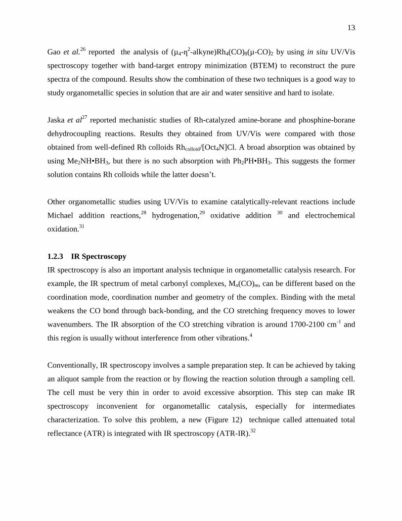
characterization. To solve this problem, a new (Figure 12) technique called attenuated total
reflectance (ATR) is integrated with IR spectroscopy (ATR-IR).32
14
ATR-IR is based on a mechanism that when the infrared beam reaches the solution surface, part
of the light will go into the solution and reflect back. The reflected IR beam contains IR
information of the solution that can be used for characterization of the solution. This technique
allows in situ IR tests directly in the reaction solution without the need to take a sample.
Figure 12: Attenuated Total Reflectance (ATR).
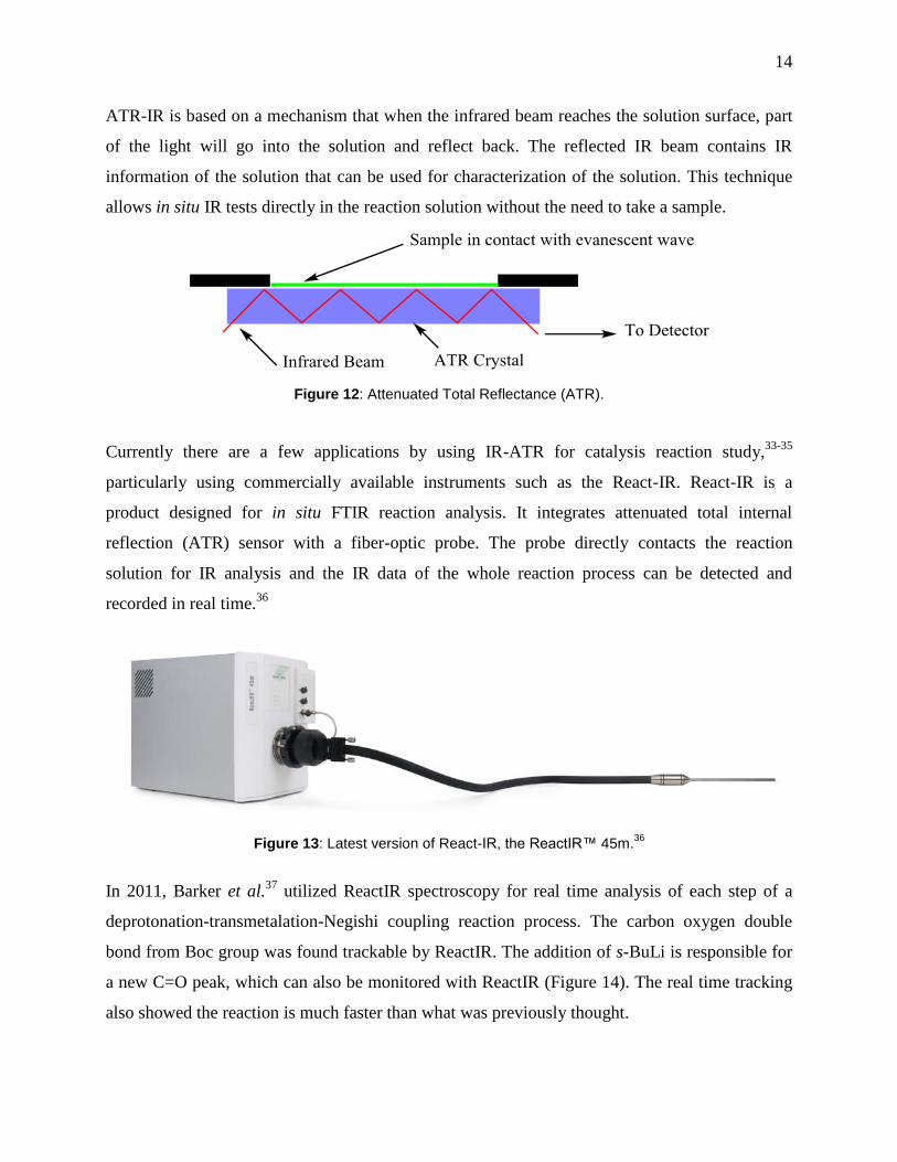
Currently there are a few applications by using IR-ATR for catalysis reaction study,33-35
particularly using commercially available instruments such as the React-IR. React-IR is a
product designed for in situ FTIR reaction analysis. It integrates attenuated total internal
reflection (ATR) sensor with a fiber-optic probe. The probe directly contacts the reaction
solution for IR analysis and the IR data of the whole reaction process can be detected and
recorded in real time.36
Figure 13: Latest version of React-IR, the ReactIR™ 45m.
36
In 2011, Barker et al.37
utilized ReactIR spectroscopy for real time analysis of each step of a
deprotonation-transmetalation-Negishi coupling reaction process. The carbon oxygen double
bond from Boc group was found trackable by ReactIR. The addition of s-BuLi is responsible for
a new C=O peak, which can also be monitored with ReactIR (Figure 14). The real time tracking
also showed the reaction is much faster than what was previously thought.

15
Figure 14: ReactIR spectrum of lithiation of N-Boc pyrrolidine compound.37
Reprinted with permission
from “Enantioselective, Palladium-Catalyzed α-Arylation of N-Boc Pyrrolidine: In Situ React IR
Spectroscopic Monitoring, Scope, and Synthetic Applications” G. Barker, J. L. McGrath, A. Klapars, D.
Stead, G. Zhou, K. R. Campos and P. O’Brien, The Journal of Organic Chemistry, 2011, 76, 5936-5953.
Copyright © 2011 American Chemical Society
In 2013, Gall et al.38
reported using in situ infrared spectroscopy tracking of a Mannich-like
reaction between amines, aldehydes and organozinc reagents by using ReactIR (Figure 15). In
order to track different starting materials, products and intermediates, most of these species were
first characterized individually. The authors managed to obtain enough information from
spectroscopic data to propose two different pathways for the reaction, however, the key
intermediate species are hard to identify due to stability issues.

16
Figure 15: Overlay of different spectra including starting reagents, product and putative imine
intermediate.38
Reprinted with permission from “Mannich-like three-component synthesis of α-branched
amines involving organozinc compounds: ReactIR monitoring and mechanistic aspects” E. Le Gall, S.
Sengmany, C. Hauréna, E. Léonel and T. Martens, Journal of Organometallic Chemistry, 2013, 736, 27-
35. Copyright © 2013 Elsevier B.V.
1.2.4 Mass Spectrometry
A mass spectrometer converts a sample into gas phase ions, and electric (and sometimes
magnetic) fields are applied to separate the ions by their mass-to-charge ratio.39 Mass
spectrometry is an outstanding analytical technique due to its high sensitivity (low detection
limit),40
high accuracy and the low amount of analyte it requires. With modern soft ionization
techniques, MALDI (Matrix Assisted Laser Desorption Ionisation) –left side of Figure 16 and,
ESI (Electrospray Ionisation) –right side of Figure 16 41, 42
little or even no fragmentation occurs
during ionisation process, thus allowing the intact target molecule to be characterized.

17
Figure 16: MALDI (left) and ESI sources.41, 42
Reprinted with permission from “Electrospray and MALDI
Mass Spectrometry: Fundamentals, Instrumentation, Practicalities, and Biological Applications, Second
Edition” R. B. Cole, Electrospray and MALDI Mass Spectrometry: Fundamentals, Instrumentation,
Practicalities, and Biological Applications, John Wiley & Sons, 2009. Copyright © 2010 John Wiley &
Sons, Inc.
ESI-MS has become an increasingly popular tool for mechanistic studies of organometallic
catalysis, especially in the area of short-lived reactive intermediates.43
The reaction solution can
be directly introduced into the instrument without pre-treatment. A more important advantage is
that ESI-MS can quantitatively detect short life time, low concentration, and air-sensitive
intermediates. However, in order to be detectable by MS, the species must be intrinsically
charged such as a positive or negative ion. The synthetic introduction of charged tags into the
target molecule is one of the best ways to achieve this goal. Currently ESI-MS has been
successfully used in the study of catalytic oxidation,44-46
palladium cross-coupling,47-49
the
Pauson-Khand reaction,50
and many other reactions.51-57
Santos et al.58
reported a mechanistic investigation of a Lewis base-catalyzed Baylis-Hillman
reaction by using ESI-MS. The reason to use ESI-MS for this reaction is that the key
intermediates in the proposed Baylis-Hillman reaction catalytic cycle (Figure 17) are
monocations. The reaction intermediates as shown in Figure 17 can be transformed into gas
phase and characterized by ESI-MS. The final results of Santos et al. confirmed this proposal.

18
Figure 17: ESI-MS study of the mechanism of a Baylis-Hillman reaction catalyzed by DABCO.58
Shvo’s catalyst59
is a ruthenium complex reported as capable of achieving chemo-enzymatic
dynamic kinetic resolution (DKR) of amines. Evidence of an intermediate from the proposed
mechanism was characterized by NMR and IR, however, many key intermediates had not been
detected, and there were two different pathways proposed. In order to find out the correct
pathway, Vaz et al.60
investigated this reaction by using ESI-MS and ESI-MS/MS. Many
intermediates were captured and characterized (Figure 18), and the reaction process was
continuously monitored. Results show evidence to support an inner-sphere H-transfer
mechanism (Figure 19).

19
Figure 18: Charged intermediates were detected during the DKR of amines reaction, each intermediate
can be represented by a characteristic peak.60
Reprinted with permission from “Shvo's catalyst in
chemoenzymatic dynamic kinetic resolution of amines – inner or outer sphere mechanism?” B. G. Vaz, C.
D. F. Milagre, M. N. Eberlin and H. M. S. Milagre, Organic & Biomolecular Chemistry, 2013, 11, 6695-
6698. Copyright © The Royal Society of Chemistry 2013
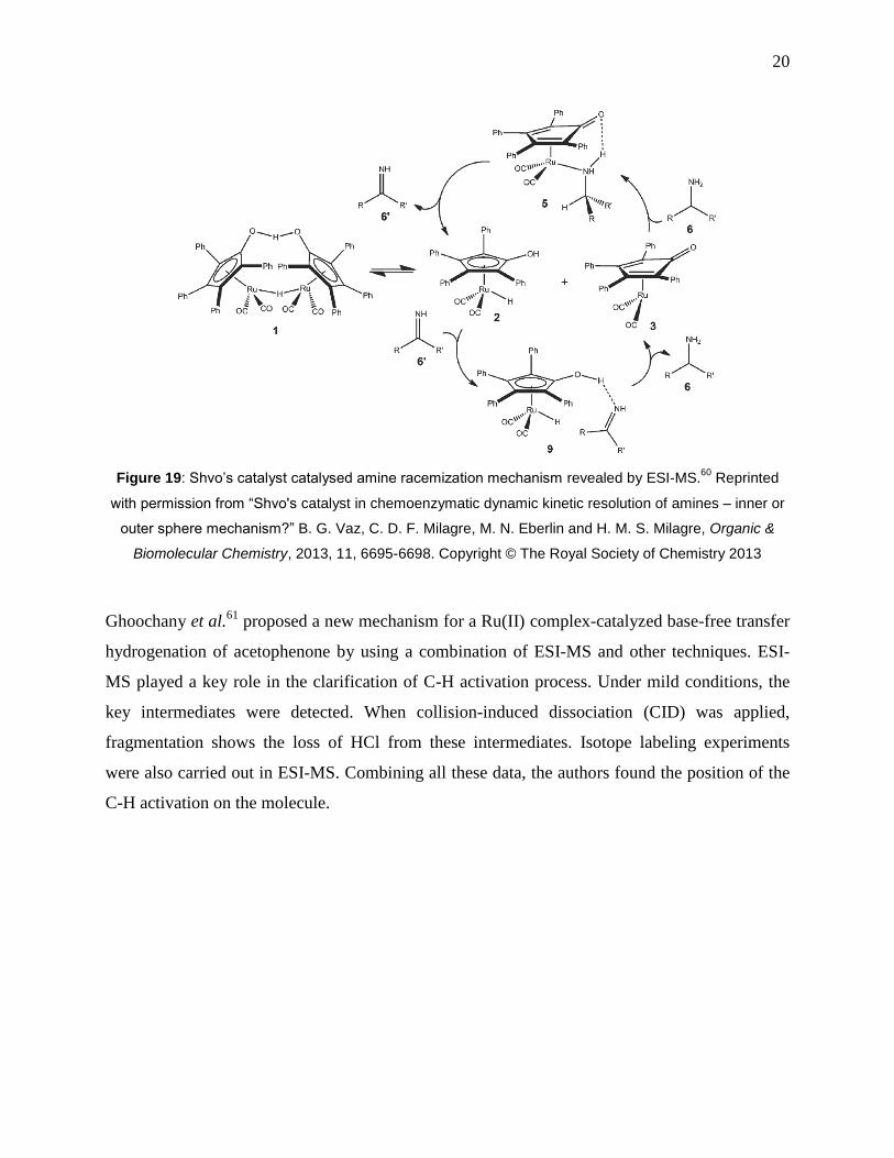
20
Figure 19: Shvo’s catalyst catalysed amine racemization mechanism revealed by ESI-MS.60
Reprinted
with permission from “Shvo's catalyst in chemoenzymatic dynamic kinetic resolution of amines – inner or
outer sphere mechanism?” B. G. Vaz, C. D. F. Milagre, M. N. Eberlin and H. M. S. Milagre, Organic &
Biomolecular Chemistry, 2013, 11, 6695-6698. Copyright © The Royal Society of Chemistry 2013
Ghoochany et al.61
proposed a new mechanism for a Ru(II) complex-catalyzed base-free transfer
hydrogenation of acetophenone by using a combination of ESI-MS and other techniques. ESI-
MS played a key role in the clarification of C-H activation process. Under mild conditions, the
key intermediates were detected. When collision-induced dissociation (CID) was applied,
fragmentation shows the loss of HCl from these intermediates. Isotope labeling experiments
were also carried out in ESI-MS. Combining all these data, the authors found the position of the
C-H activation on the molecule.
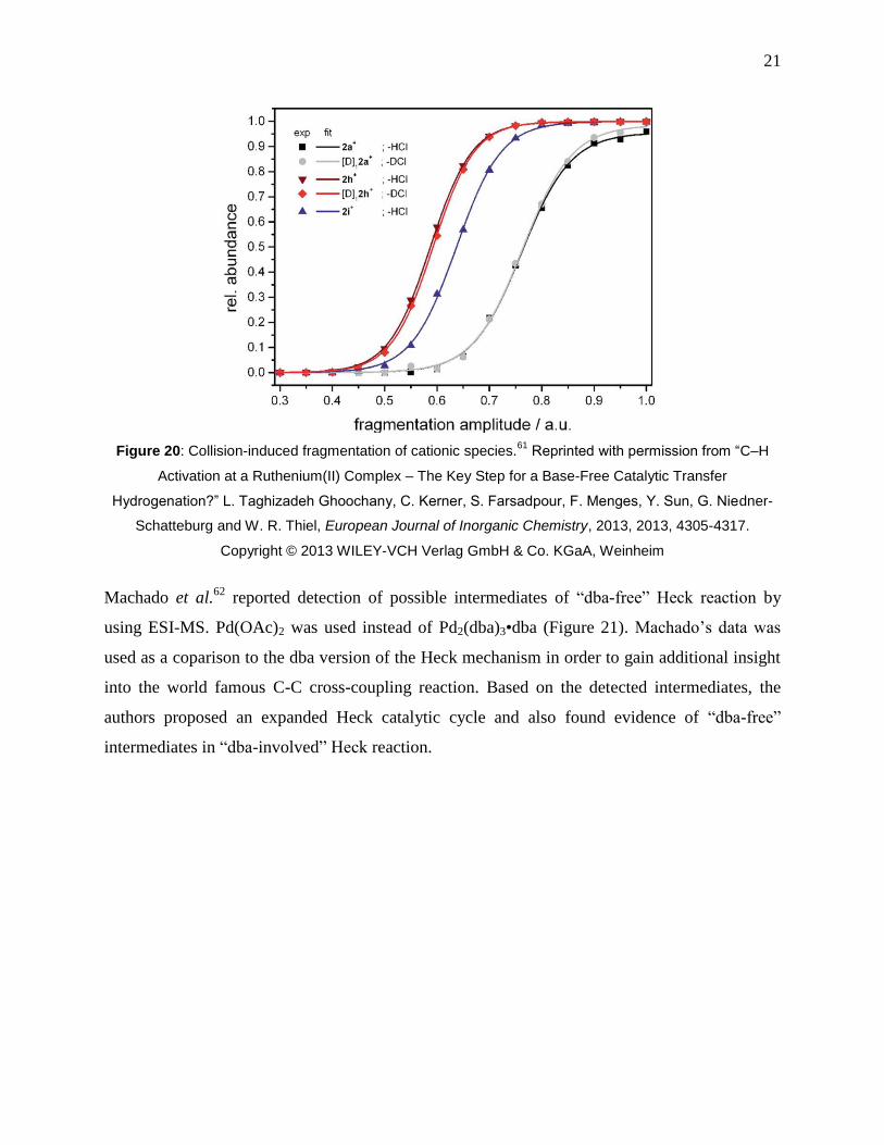
21
Figure 20: Collision-induced fragmentation of cationic species.61
Reprinted with permission from “C–H
Activation at a Ruthenium(II) Complex – The Key Step for a Base-Free Catalytic Transfer
Hydrogenation?” L. Taghizadeh Ghoochany, C. Kerner, S. Farsadpour, F. Menges, Y. Sun, G. Niedner-
Schatteburg and W. R. Thiel, European Journal of Inorganic Chemistry, 2013, 2013, 4305-4317.
Copyright © 2013 WILEY-VCH Verlag GmbH & Co. KGaA, Weinheim
Machado et al.62
reported detection of possible intermediates of “dba-free” Heck reaction by
using ESI-MS. Pd(OAc)2 was used instead of Pd2(dba)3•dba (Figure 21). Machado’s data was
used as a coparison to the dba version of the Heck mechanism in order to gain additional insight
into the world famous C-C cross-coupling reaction. Based on the detected intermediates, the
authors proposed an expanded Heck catalytic cycle and also found evidence of “dba-free”
intermediates in “dba-involved” Heck reaction.
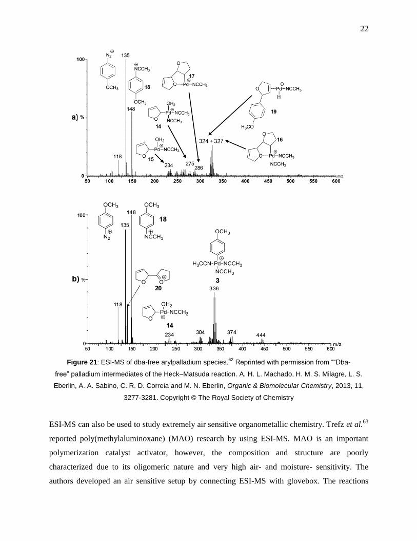
22
Figure 21: ESI-MS of dba-free arylpalladium species.62
Reprinted with permission from ““Dba-
free” palladium intermediates of the Heck–Matsuda reaction. A. H. L. Machado, H. M. S. Milagre, L. S.
Eberlin, A. A. Sabino, C. R. D. Correia and M. N. Eberlin, Organic & Biomolecular Chemistry, 2013, 11,
3277-3281. Copyright © The Royal Society of Chemistry
ESI-MS can also be used to study extremely air sensitive organometallic chemistry. Trefz et al.63
reported poly(methylaluminoxane) (MAO) research by using ESI-MS. MAO is an important
polymerization catalyst activator, however, the composition and structure are poorly
characterized due to its oligomeric nature and very high air- and moisture- sensitivity. The
authors developed an air sensitive setup by connecting ESI-MS with glovebox. The reactions
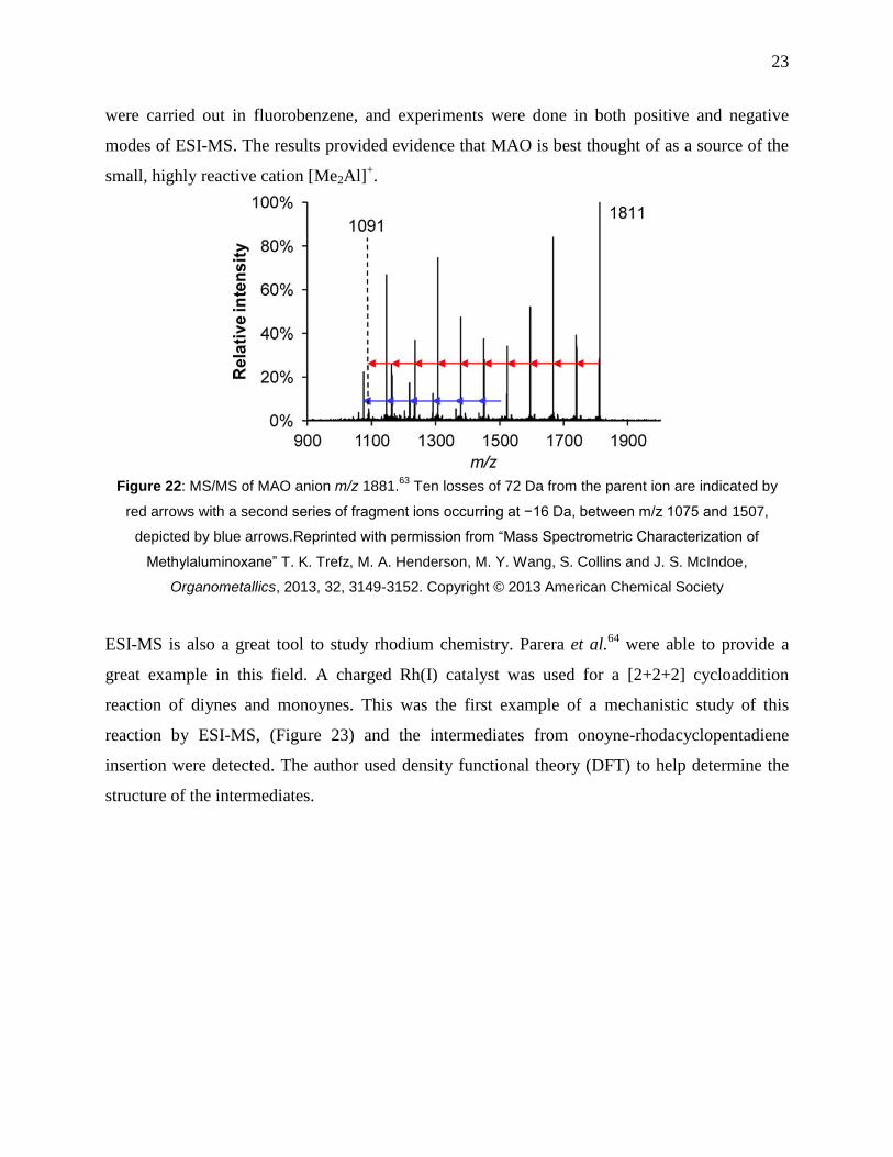
23
were carried out in fluorobenzene, and experiments were done in both positive and negative
modes of ESI-MS. The results provided evidence that MAO is best thought of as a source of the
small, highly reactive cation [Me2Al]+.
Figure 22: MS/MS of MAO anion m/z 1881.63
Ten losses of 72 Da from the parent ion are indicated by
red arrows with a second series of fragment ions occurring at −16 Da, between m/z 1075 and 1507,
depicted by blue arrows.Reprinted with permission from “Mass Spectrometric Characterization of
Methylaluminoxane” T. K. Trefz, M. A. Henderson, M. Y. Wang, S. Collins and J. S. McIndoe,
Organometallics, 2013, 32, 3149-3152. Copyright © 2013 American Chemical Society
ESI-MS is also a great tool to study rhodium chemistry. Parera et al.64
were able to provide a
great example in this field. A charged Rh(I) catalyst was used for a [2+2+2] cycloaddition
reaction of diynes and monoynes. This was the first example of a mechanistic study of this
reaction by ESI-MS, (Figure 23) and the intermediates from onoyne-rhodacyclopentadiene
insertion were detected. The author used density functional theory (DFT) to help determine the
structure of the intermediates.
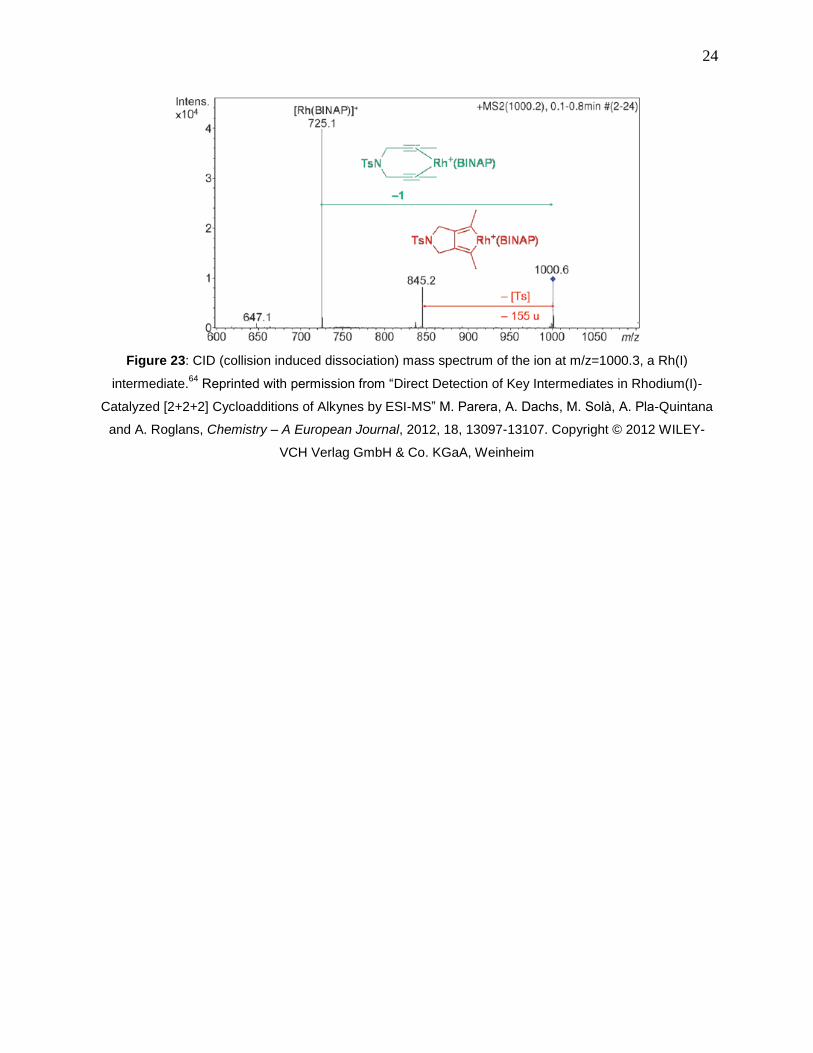
24
Figure 23: CID (collision induced dissociation) mass spectrum of the ion at m/z=1000.3, a Rh(I)
intermediate.64
Reprinted with permission from “Direct Detection of Key Intermediates in Rhodium(I)-
Catalyzed [2+2+2] Cycloadditions of Alkynes by ESI-MS” M. Parera, A. Dachs, M. Solà, A. Pla-Quintana
and A. Roglans, Chemistry – A European Journal, 2012, 18, 13097-13107. Copyright © 2012 WILEY-
VCH Verlag GmbH & Co. KGaA, Weinheim

25
2. Techniques and methodologies
2.1 Introduction
Mass spectrometry is a classic technique in analytical chemistry. It has three main components:
1, the ion source where sample molecules get ionized and converted into gas phase charged
particles; 2, the mass analyzer where ions are sorted and separated based on their mass-to-charge
ratio (m/z); 3, the detector, where the sorted ions are counted to get the ion intensity.
Mass spectrometry is originated from the field of physics; in the early 1900’s the research of J.J
Thomson on cathode rays established the foundation of MS field. Together with Francis Aston,
he built the world’s first mass spectrometer for atom mass measurement.65
Since then, different
types of mass spectrometer were created. All the three components of MS have been constantly
innovated over the past 110 years.
The first ionization source was electron ionization (EI) developed by Dempster.66
In the EI
source, when vaporized sample molecules pass through a beam of high energy electrons, an
electron of the analyte molecule is forced out of its orbital due to the powerful external electron
beam. This leads to the production of the molecular ion [M]•+
. This ionization process is so
energetic that only a very small portion of intact sample molecules can survive and the spectrum
contains mainly fragments of the parent ion.
Since this method only gives limited information on the parent molecule, “soft” ionization
methods were developed. Chemical ionization (CI)67, 68
utilizes a reagent gas as a bridge between
a highly energized electron beam and sample molecules, so the charge transfer is not directly
between electron beam and sample which is the case of EI. In CI at first the electron beam hits
the reagent gas (e.g. CH4) to ionize it, which then charge transfered to the adjacent analyte. As
there is no direct contact between beam and sample, the fragmentation of the analyte is decreased
significantly; more parent ion data can be obtained, but CI still has limited ability to detect large
molecules because, like EI, it is limited by sample volatility.
Many other ionization methods were developed as well, such as Field Desorption (FD)69
, Fast
Atom Bombardment (FAB)70, 71
, and Atmospheric Pressure Chemical Ionization (APCI)72
etc.
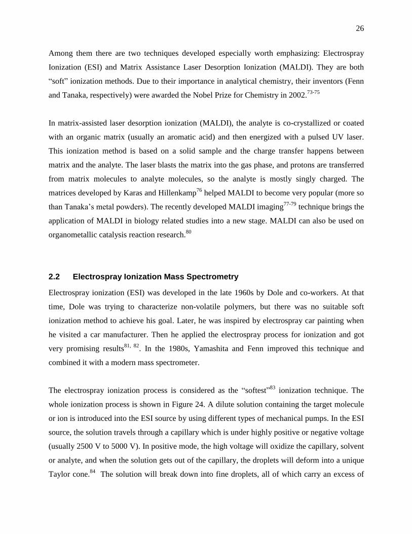
26
Among them there are two techniques developed especially worth emphasizing: Electrospray
Ionization (ESI) and Matrix Assistance Laser Desorption Ionization (MALDI). They are both
“soft” ionization methods. Due to their importance in analytical chemistry, their inventors (Fenn
and Tanaka, respectively) were awarded the Nobel Prize for Chemistry in 2002.73-75
In matrix-assisted laser desorption ionization (MALDI), the analyte is co-crystallized or coated
with an organic matrix (usually an aromatic acid) and then energized with a pulsed UV laser.
This ionization method is based on a solid sample and the charge transfer happens between
matrix and the analyte. The laser blasts the matrix into the gas phase, and protons are transferred
from matrix molecules to analyte molecules, so the analyte is mostly singly charged. The
matrices developed by Karas and Hillenkamp76
helped MALDI to become very popular (more so
than Tanaka’s metal powders). The recently developed MALDI imaging77-79
technique brings the
application of MALDI in biology related studies into a new stage. MALDI can also be used on
organometallic catalysis reaction research.80
2.2 Electrospray Ionization Mass Spectrometry
Electrospray ionization (ESI) was developed in the late 1960s by Dole and co-workers. At that
time, Dole was trying to characterize non-volatile polymers, but there was no suitable soft
ionization method to achieve his goal. Later, he was inspired by electrospray car painting when
he visited a car manufacturer. Then he applied the electrospray process for ionization and got
very promising results81, 82
. In the 1980s, Yamashita and Fenn improved this technique and
combined it with a modern mass spectrometer.
The electrospray ionization process is considered as the “softest”83
ionization technique. The
whole ionization process is shown in Figure 24. A dilute solution containing the target molecule
or ion is introduced into the ESI source by using different types of mechanical pumps. In the ESI
source, the solution travels through a capillary which is under highly positive or negative voltage
(usually 2500 V to 5000 V). In positive mode, the high voltage will oxidize the capillary, solvent
or analyte, and when the solution gets out of the capillary, the droplets will deform into a unique
Taylor cone.84
The solution will break down into fine droplets, all of which carry an excess of

27
positive charge. As the charges repel each other, they will all relocate on the surface of the fine
droplet. During the flying of the droplets, they are surrounded by a warm drying gas which will
help solvent molecules evaporate. This evaporation will cause the charge density of the droplet
to increase and once the charge density reaches a Coulomb explosion threshold, the droplet split
into smaller droplets with lower charge density, this splitting process will repeatedly occur in a
very short time frame.85
Eventually, all the solvent molecules evaporate and the positive charges
stay with sample molecule ions in gas phase and enter into the MS analyzer.
Figure 24: The desolvation process in electrospray ionization. Modified with permission of the author from
Henderson, W., McIndoe J. S., Mass Spectrometry of Inorganic and Organometallic Compounds. John
Wiley & Sons, Ltd. West Sussex: 2005, p. 92.
When the target molecules are separated from the rest of solvent molecules, there are two models
to explain this final stage of ionization. The Ion Evaporation Model (IEM) and Charged Residue
Model (CRM).86
Small ions (<5000 Da) tend to transfer into the gas phase by evaporating from
the surface of droplet, while large ions are likely to stay inside the droplet until all the
surrounding solvent molecules evaporate(Figure 25). The whole process of ESI enables the
target molecule to stay intact rather than generate many fragments. So information of the intact
molecule can be captured.
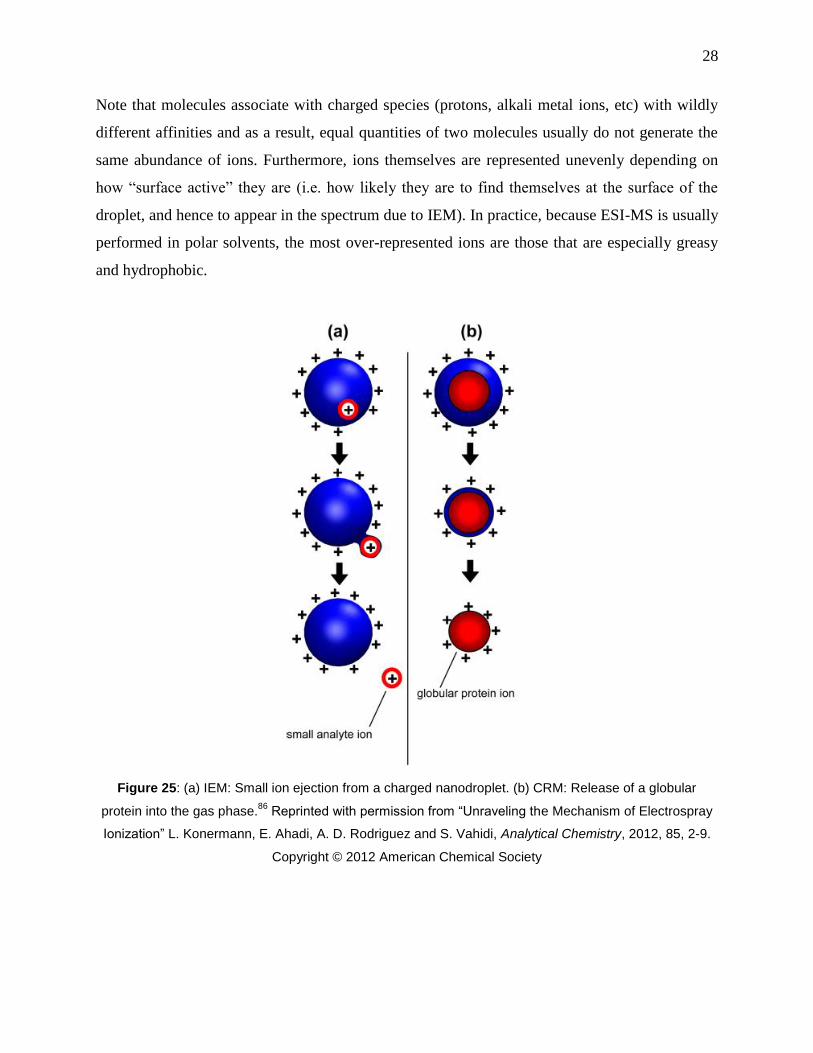
28
Note that molecules associate with charged species (protons, alkali metal ions, etc) with wildly
different affinities and as a result, equal quantities of two molecules usually do not generate the
same abundance of ions. Furthermore, ions themselves are represented unevenly depending on
how “surface active” they are (i.e. how likely they are to find themselves at the surface of the
droplet, and hence to appear in the spectrum due to IEM). In practice, because ESI-MS is usually
performed in polar solvents, the most over-represented ions are those that are especially greasy
and hydrophobic.
Figure 25: (a) IEM: Small ion ejection from a charged nanodroplet. (b) CRM: Release of a globular
protein into the gas phase.86
Reprinted with permission from “Unraveling the Mechanism of Electrospray
Ionization” L. Konermann, E. Ahadi, A. D. Rodriguez and S. Vahidi, Analytical Chemistry, 2012, 85, 2-9.
Copyright © 2012 American Chemical Society

29
2.3 Quadrupole –Time of Flight (Q-TOF)
The ESI instrument used in this work was a Waters Q-TOF-Micro tandem mass spectrometer.
Once gas phase ions are generated from the ESI source, they will be drawn into the sample cone
due to the pressure difference as shown in Figure 26. The ESI source chamber is under slightly
higher than atmospheric pressure, but the pressure inside of the sample cone is much lower. As
from this part, the MS machine is under vacuum. Voltage difference is another driving force for
the ion traveling process. However, not all of the ions get into the sample cone; a large
proportion hits the cleanable baffle. If small droplets get into the sample cone, remaining solvent
will be evaporated and pumped away. After that, ions traverse a right angle turn and enter the
extraction cone which leads to an RF hexapole. RF lens chamber and analyzer part is under high
vacuum (2 × 10⁻⁷
mbar). This setup is to make sure there is a minimum amount of neutral
molecules get into the analyzer.
Figure 26: Electrospray source with QTOF-Micro scheme.87
Reprinted with permission from “Micromass
Q-TOF micro Mass Spectrometer Operator’s Guide” Copyright © 2012 Waters Corporation
As shown in Figure 27,87
ions pass through a hexapole RF lens, in this part, ions will be confined
into a narrow beam. In the next step, ions will enter into pre-filter, to get rid of low mass
molecules before they enter the main quadrupole analyser as shown in Figure 28.87
30
Figure 27: The Ion Optical System of the Q-TOF micro.87
Reprinted with permission from “Micromass Q-
TOF micro Mass Spectrometer Operator’s Guide” Copyright © 2012 Waters Corporation

31
Figure 28: The Prefilter and Main Analyzer of the Q-TOF micro87
Reprinted with permission from
“Micromass Q-TOF micro Mass Spectrometer Operator’s Guide” Copyright © 2012 Waters Corporation
The quadrupole analyzer has two functions. First, it can be used to focus on a specific m/z range,
for example, from m/z 50 to 2000. Second, it can be used to focus on a target m/z value, this is
useful for MS/MS analysis, in other word, analyze the product ions by using collision induced
dissociation (CID) to break the precursor ions apart.
Before ions enter the Time Of Flight analyzer, they will pass through collision gas cell, which
contains Ar gas. Collision Induced Dissociation (CID) happens in this cell. In MS mode, this gas
cell just works as a hexapole RF lens to help ions pass through to the second analyzer, but in
MS/MS mode, the collision voltage can be set to higher value and this will lead to higher
collision energy, and the ions will start generating fragments as the ions hit the collision gas and
break apart. And the fragments will provide important structural information of the parent ions.
CID can also provide bond strength information; there are different types of bonds inside a
molecule, the bond strength information can be detected by CID. Stronger bonds take higher
collision energy to break. Energy dependent ESI (EDESI) is an important type of reaction that
can be achieved by CID. EDESI is shown as contour map, on this map, the m/z of a give ion will
be shown as well as the stability of each fragment at a certain collision voltage (Figure 29).88 It
provides information about bonding strength of ligands for a target molecule.

32
Figure 29 Positive-ion energy-dependent ESI-MS of a representative example. X axis is the m/z, Y axis is
collision energy in voltage, the red and blue dots are the detected signal of a certain species at the
applied voltage.88
Reprinted with permission from “Synthesis and characterization of a new class of anti-
angiogenic agents based on ruthenium clusters” A. A. Nazarov, M. Baquié, P. Nowak-Sliwinska, O. Zava,
J. R. van Beijnum, M. Groessl, D. M. Chisholm, Z. Ahmadi, J. S. McIndoe, A. W. Griffioen, H. van den
Bergh and P. J. Dyson, Sci. Rep., 2013, 3. Copyright © 2013 Macmillan Publishers Limited
In the next step, ions will enter into an orthogonal time-of-flight analyzer. When ions reach a
device called the pusher, they are pulsed down a flight tube in a perpendicular direction.
However, same mass-to-charge ratio ions within each group may contain different kinetic energy
and their moving directions are also different, these must be corrected before they hit detector,
otherwise the mass accuracy will suffer. The reflectron is the device to correct this; it works like
an ion mirror, repelling ions back down the flight tube, as shown in Figure 30. Ions with higher
kinetic energy will travel deeper into the reflectron than those with lower kinetic energy. After
the reflection, the ions with same m/z will all hit the ion detector at the same time.

33
Figure 30 Time of Flight analyzer87
Reprinted with permission from “Micromass Q-TOF micro Mass
Spectrometer Operator’s Guide” Copyright © 2012 Waters Corporation
The microchannel plate detector (MCP) is the final destination for the ions. It contains thousands
of electron multipliers. When an ion hits the MCP, it will trigger an electron multiplier to
generate a current. The strength of the current depends on the number of ions that arrives at
MCP. Ions arrive at the same time have the same m/z. The more ions that arrive at the same time,
the stronger the current will be, and it will be converted into computer data for future processing.
The output signal will be transferred into Waters’ analysis software MassLynx where ion
intensity and m/z is displayed in a Microsoft Windows system.
2.4 Continuous reaction monitoring with ESI-MS
ESI-MS cannot only detect the m/z of a target analyte, it can also detect the quantity of it in a
given reaction because the MCP can detect both ion mass-to-charge ratio and ion intensity. The
ion intensity represents the number of analytes which reach the MCP and this number is
proportional to the concentration of the analyte in solution. When analyte concentration changes,
34
ion intensity also changes, it makes ESI-MS a perfect instrument for tracking target species in a
dynamic reaction.
All the analytical techniques introduced in Chapter 1 can be used to track the whole process of a
reaction. However, ESI-MS has unique advantages over all the other instruments in
organometallic catalytic reactions. Any catalytic reaction can be a complicated mixture; it
contains starting materials, catalysts, different intermediates, products and by-products as well as
decomposed compounds. Usually the catalyst has low concentration, all of the compounds are in
a dynamic environment which changes every second. It requires instrument with ability to detect,
identify and track all the individual species in real time with very short interval time between
each sampling (per second). In some cases, the reactions are air and moisture sensitive and the
sample has to be protected under inert atmosphere. Mass spectrometry is an appropriate
technique to achieve all of these goals.
Continuous reaction monitoring can be carried out using a technique called pressurized sample
infusion (PSI) which was invented and developed by our previous group member Dr. Krista
Vikse89, 90
. The setup is shown in Figure 31. PSI is a cannula system that transfers a small
amount of continuously flowing reaction solution from a slightly pressurized (1-10 psi) Schlenk
flask to ESI-MS through PEEK tubing.
The pressure source of the system can be different depend on what the type of reaction to be
monitored. For air and moisture sensitive reactions, the gas can be N2 or Ar; for hydrogenation
reaction H2 will be used. Other examples include O2, CO, condensed air, CO2, C2H4 etc. The
flow rate based on the flask pressure and tube length and diameter was calculated based on the
Hagen-Poiseuille equation, and tested under practical conditions.72
The ideal pressure is 3 psi
which is calculated based on Hagen–Poiseuille equation,91
this pressure allows us to obtain a
flowrate 30 to 60µL per minute. The pressure can be also set from 1 to 10 psi based on different
reaction purposes.
The Schlenk flask is the reaction container, so for reactions that require high temperature, a
condenser is necessary for cooling. The Schlenk flask has to be well sealed if the reaction is air

35
sensitive. Rubber septa and Teflon tape are commonly used. Grease can also be used but with
caution as it can dissolve in certain solvent to interfere with reactions.
Figure 31 Pressurized sample infusion system setup.
A short length of PEEK tubing (0.4 m) is used for cannula transfer. If the concentration of the
reaction solution is too high, it can saturate the MS detector. In such cases, an online dilution
system can be installed by using a T-piece. Diluting solvent can decrease the concentration to 1%
of the original concentration. If the dilution solvent is different from reaction solvent or same
solvent but with different temperature, it will help to quench the reaction, so the reaction will be
stopped at the T-piece but the flow will keep going.
Once the system is set up, the reaction solution will be pushed into ESI-MS by the slight over
pressure. Sampling time is set to 1 second per spectrum in most cases. The absolute intensity of
each species in the reaction will be normalized against total ion current. An example of standard
PSI-ESI-MS continuous reaction monitoring result is shown in Figure 32.72
In this example, we

36
can see a silane redistribution reaction. When the catalyst is added; the starting material is
converted into product over time.
Figure 32: Normalized intensity vs. time trace for a charged silane (m/z 349) and appearance of the
product of redistribution (m/z 425).72

37
3. Methodological innovations
3.1 Numerical modeling
In order to simulate the proposed catalytic reaction mechanism and match the simulation with
experimental result, we used different computer programs: Powersim92
and COPASI93
.
Powersim is system dynamic software originally used for financial and business simulation. But
we chemists found a way to run reaction related simulations with it(Figure 33) 94-96
. The reasons
that chemists can use financial software for chemistry kinetic studies is because Powersim
simulation pathway design is based on graphic symbols and arrows rather than lines of codes as
in Maple (Maplesoft Inc). And Powersim models can be built based on pure methametical
equations, chemical reaction process can be converted into these equations as elemental steps.
This saves a lot of time not having to learn a programming language. With a few hours’ design,
a Powersim numerical model can be built (Figure 34) based on a proposed mechanism (Figure
33).
Figure 33: Proposed mechanism for hydrogenation of alkyne by Wilkinson’s catalyst.95

38
Figure 34: Powersim Numerical model
95, this figure represents a Wilkinson’s hydrogenation reaction.
After a Powersim model is built, the next step is rate constants estimation. This is the most
difficult part for establishing a good model. For a proposed mechanism, the reasonable way to
estimate a rate constant is to do literature research on related reactions and specific studies on a
specific step of the whole reaction, and for rest of the steps, manual optimization is required. By
appearance of simulated results, the rate constants will be revised to make it fit better into the
experiment results.
Another numerical modeling software that we are using is called COPASI93
. It stands for
COmplex PAthway SImulator. COPASI is open-source software which can be downloaded from
the authors’ website. COPASI has a simple interface and it is designed for biology and chemistry
related simulations.

39
Figure 35: COPASI interface
For the same reversible reaction:
all you need to do is to type in a few characters, in this example, the model is A + B = C + D, the
symbol “=” means it is a reversible reaction. If it is irreversible, we can use “->” instead of “=”.

40
Figure 36: COPASI model for reversible reaction
COPASI allows users to import real reaction data and do automatic matching calculations based
on different mathematical methods (Figure 37) to find the rate constants that best fit the reaction.
The software will do 30-100 calculations per second. Based on the complexity of the model, the
whole calculation process may last from a few seconds to hours. This function is very important
for rate constants optimization and it can speed up the whole model building process greatly.
While does not have the graphical user interface of Powersim overall it is a much more powerful
tool for building numerical models for catalytic mechanisms.
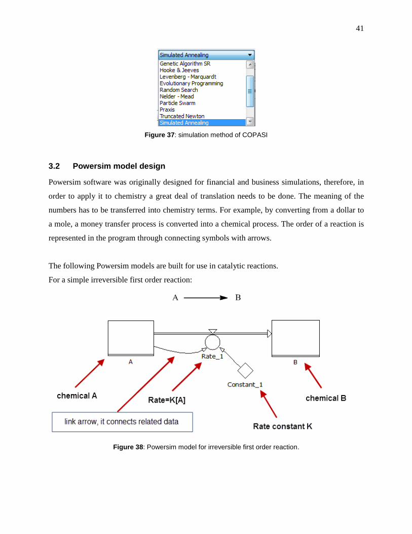
41
Figure 37: simulation method of COPASI
3.2 Powersim model design
Powersim software was originally designed for financial and business simulations, therefore, in
order to apply it to chemistry a great deal of translation needs to be done. The meaning of the
numbers has to be transferred into chemistry terms. For example, by converting from a dollar to
a mole, a money transfer process is converted into a chemical process. The order of a reaction is
represented in the program through connecting symbols with arrows.
The following Powersim models are built for use in catalytic reactions.
For a simple irreversible first order reaction:
Figure 38: Powersim model for irreversible first order reaction.
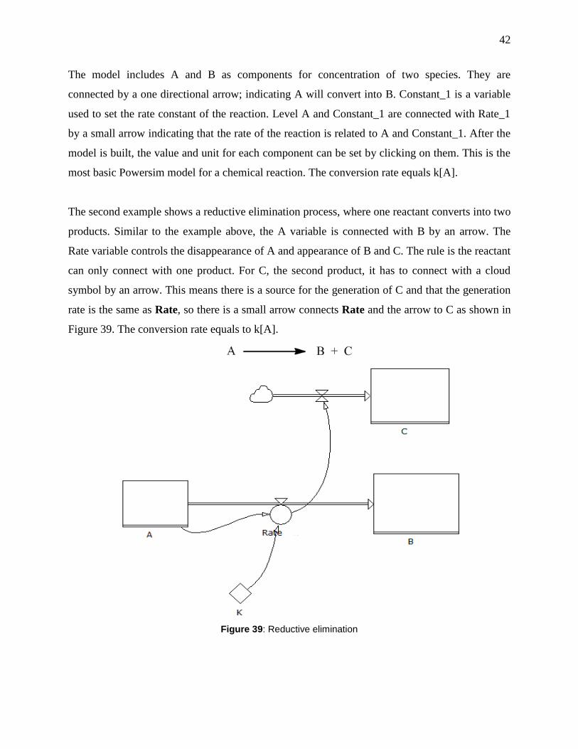
42
The model includes A and B as components for concentration of two species. They are
connected by a one directional arrow; indicating A will convert into B. Constant_1 is a variable
used to set the rate constant of the reaction. Level A and Constant_1 are connected with Rate_1
by a small arrow indicating that the rate of the reaction is related to A and Constant_1. After the
model is built, the value and unit for each component can be set by clicking on them. This is the
most basic Powersim model for a chemical reaction. The conversion rate equals k[A].
The second example shows a reductive elimination process, where one reactant converts into two
products. Similar to the example above, the A variable is connected with B by an arrow. The
Rate variable controls the disappearance of A and appearance of B and C. The rule is the reactant
can only connect with one product. For C, the second product, it has to connect with a cloud
symbol by an arrow. This means there is a source for the generation of C and that the generation
rate is the same as Rate, so there is a small arrow connects Rate and the arrow to C as shown in
Figure 39. The conversion rate equals to k[A].
Figure 39: Reductive elimination
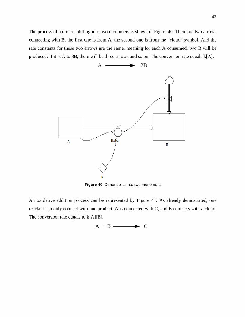
43
The process of a dimer splitting into two monomers is shown in Figure 40. There are two arrows
connecting with B, the first one is from A, the second one is from the “cloud” symbol. And the
rate constants for these two arrows are the same, meaning for each A consumed, two B will be
produced. If it is A to 3B, there will be three arrows and so on. The conversion rate equals k[A].
Figure 40: Dimer splits into two monomers
An oxidative addition process can be represented by Figure 41. As already demostrated, one
reactant can only connect with one product. A is connected with C, and B connects with a cloud.
The conversion rate equals to k[A][B].
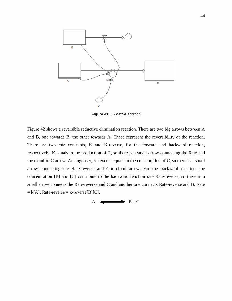
44
Figure 41: Oxidative addition
Figure 42 shows a reversible reductive elimination reaction. There are two big arrows between A
and B, one towards B, the other towards A. These represent the reversibility of the reaction.
There are two rate constants, K and K-reverse, for the forward and backward reaction,
respectively. K equals to the production of C, so there is a small arrow connecting the Rate and
the cloud-to-C arrow. Analogously, K-reverse equals to the consumption of C, so there is a small
arrow connecting the Rate-reverse and C-to-cloud arrow. For the backward reaction, the
concentration [B] and [C] contribute to the backward reaction rate Rate-reverse, so there is a
small arrow connects the Rate-reverse and C and another one connects Rate-reverse and B. Rate
= k[A], Rate-reverse = k-reverse[B][C].

45
Figure 42: Reversible reductive elimination
For the following reaction:

46
Figure 43: Powersim model for second order reversible reaction.
In this second order reversible reaction, we have two reactants and two products. When we try to
build this model, the first step is to connect one reactant with one product. In this example, A
connects with C, and B connects with D. There are 2 big arrows between A and C in two
directions, which means A can convert into C and C can convert back into A. B is involved in
the A-C conversion, so A, B and rate constant k are all connected with Rate. The Rate controls
the decrease of A and B and increase of C and D. For the reverse reaction, it is the same method.
Rate=k[A][B], Rate-reverse=k-reverse[C][D].
For a complicated catalytic mechanism, these six elementary reactions make up the building
blocks of the catalytic cycle.
3.3 Handling air and moisture sensitive reactions
When investigating air and moisture sensitive catalytic reactions using ESI-MS, there is a high
chance the sample will be exposed to air. The analyser and detector are under vacuum, but the
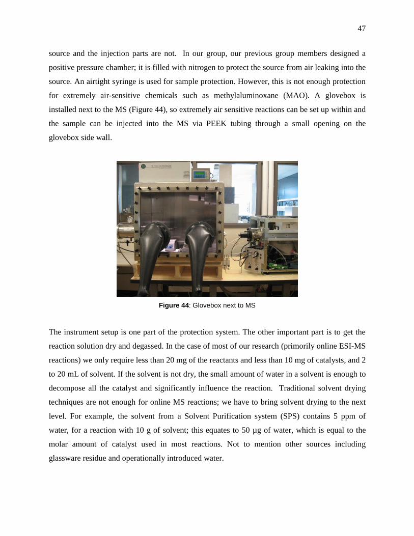
47
source and the injection parts are not. In our group, our previous group members designed a
positive pressure chamber; it is filled with nitrogen to protect the source from air leaking into the
source. An airtight syringe is used for sample protection. However, this is not enough protection
for extremely air-sensitive chemicals such as methylaluminoxane (MAO). A glovebox is
installed next to the MS (Figure 44), so extremely air sensitive reactions can be set up within and
the sample can be injected into the MS via PEEK tubing through a small opening on the
glovebox side wall.
Figure 44: Glovebox next to MS
The instrument setup is one part of the protection system. The other important part is to get the
reaction solution dry and degassed. In the case of most of our research (primorily online ESI-MS
reactions) we only require less than 20 mg of the reactants and less than 10 mg of catalysts, and 2
to 20 mL of solvent. If the solvent is not dry, the small amount of water in a solvent is enough to
decompose all the catalyst and significantly influence the reaction. Traditional solvent drying
techniques are not enough for online MS reactions; we have to bring solvent drying to the next
level. For example, the solvent from a Solvent Purification system (SPS) contains 5 ppm of
water, for a reaction with 10 g of solvent; this equates to 50 µg of water, which is equal to the
molar amount of catalyst used in most reactions. Not to mention other sources including
glassware residue and operationally introduced water.
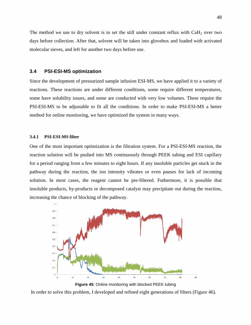
48
The method we use to dry solvent is to set the still under constant reflux with CaH2 over two
days before collection. After that, solvent will be taken into glovebox and loaded with activated
molecular sieves, and left for another two days before use.
3.4 PSI-ESI-MS optimization
Since the development of pressurized sample infusion ESI-MS, we have applied it to a variety of
reactions. These reactions are under different conditions, some require different temperatures,
some have solubility issues, and some are conducted with very low volumes. These require the
PSI-ESI-MS to be adjustable to fit all the conditions. In order to make PSI-ESI-MS a better
method for online monitoring, we have optimized the system in many ways.
3.4.1 PSI-ESI-MS filter
One of the most important optimization is the filtration system. For a PSI-ESI-MS reaction, the
reaction solution will be pushed into MS continuously through PEEK tubing and ESI capillary
for a period ranging from a few minutes to eight hours. If any insoluble particles get stuck in the
pathway during the reaction, the ion intensity vibrates or even pauses for lack of incoming
solution. In most cases, the reagent cannot be pre-filtered. Futhermore, it is possible that
insoluble products, by-products or decomposed catalyst may precipitate out during the reaction,
increasing the chance of blocking of the pathway.
Figure 45: Online monitoring with blocked PEEK tubing
In order to solve this problem, I developed and refined eight generations of filters (Figure 46).
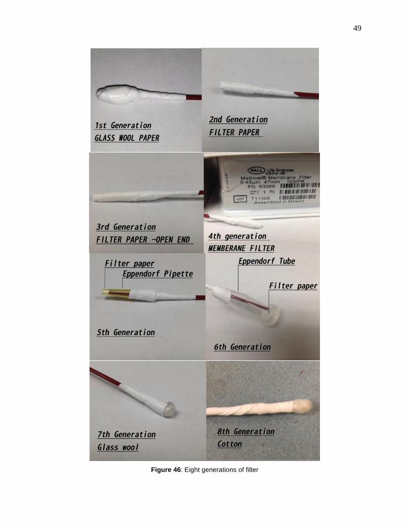
49
Figure 46: Eight generations of filter

50
Filters are made by connecting a material with PEEK tubing by Teflon tape. The ideal filter
needs to meet a few requirements. It should filter off insoluble particles, it should not
appreciably influence the flow rate or in other words increase the retention time. It should not
create an area with different concentration, and it also should not interfere with the reaction.
Based on these criteria, we can see the performance of these 8 types of filter. After years of tests,
the cotton filter was found to be the best, as different solvent can go through it quickly and the
filtration efficiency is excellent. However, cotton is still not the perfect material for all reaction
purpose, as the main component is cellulose, which contains many OH bonds and can therefore
interfere with a reactive compound such as MAO. Also, it is impossible to dry cotton in an oven
so it has to be dried by other methods. The best filter for a given scenario can be chosen by
consulting Table 2, the measurements for the performance are based on MS experimental results.
Table 2: Filter performance table
1 2 3 4 5 6 7 8
Filtration efficiency OK Bad Bad Great Great OK Great Great
Retention time Bad Great Great Great Bad Bad Bad Great
Concentration interference Ok Great Great Great OK Bad Great Great
Reaction interference No No No Yes No No No No
3.4.2 PSI-ESI-MS dilution system
A dilution system designed for a highly concentrated catalysis reaction has been designed and
tested. The detection limit of ESI-MS makes it difficult to conduct mechanistic investigations in
such concentrated solution. Our previous group members have already designed a dilution
system as shown in Figure 31, in which up to 1:100 dilution ratio can be achieved.90
However,
the problem here is that the more dilute the solution is, the more solution will pass through ESI
capillary and reach the source. This is acceptable for a short experiment but for a long reaction, it

51
will increase the degree of contamination of the instrument. In order to solve this problem and
boost the dilution efficiency, I designed a new setup (Figure 47 and Figure 48).
Figure 47: The new online dilution system.
Figure 48: Photo of online dilution system.
The adjustable splitter can be set to any ratio between the two output PEEK tubes, it is important
to protect the ESI-MS from signal overloading. With 1:100 diluted solution and a small portion
of flow, PSI-ESI-MS was tested with up to 2 M reaction solution and the test results were good
(i.e. minimal source contamination, no overloading of the detector). The larger portion of the
flow can go to collection, waste, or it can be used for other online monitoring technique
including UV and flow IR etc.
3.4.3 PSI glassware
For an air-sensitive catalytic reaction, the most-used PSI glassware is a Schlenk flask. It is
usually used for reactions with volume 2 to 50 mL. For a smaller scale reaction, it is not

52
convenient. For example, an NMR tube reaction may only contain 0.7 mL of solution and
enough solution is required to remain at the end of the reaction to allow NMR spectra to be
obtained. In order to follow the same NMR tube reaction by NMR and MS, a new PSI NMR tube
was designed. Two PEEK tubes can be plugged into a rubber NMR septum as shown in Figure
49. When low pressure is applied, the solution in the NMR tube can be infused into the mass
spectrometer. Testing results show 1 psi pressure can push 0.1 mL solution per hour. This flow
rate will not influence NMR tests so NMR and MS data can be obtained under near-identical
conditions.
Figure 49: PSI NMR tube
Air-sensitive small volume sample tests can also be done by another setup that we designed. It is
called PSI vial. The samples (trace amount to 1 mg) can be prepared in a glovebox and sealed
with septum, similar to a PSI NMR tube, and the septum is good enough to hold 3 psi pressure.

53
Figure 50: PSI sample vial. In a glovebox, small amounts of solid sample can be introduced into a vial
capped with a septum, then taken out of the glovebox and solvent injected into it. Two PEEK tubes pierce
through a septum into the vial. The yellow PEEK tube is connected to a pressure supply (e.g. Ar or N2),
and the red PEEK tube is dipped into the solution and the other end is connected to the ESI-MS. If the
sample is not soluble enough, a filter must be installed on the red PEEK tube and the septum fitted before
the vial is capped.
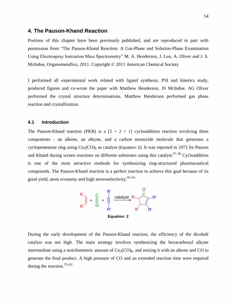
54
4. The Pauson-Khand Reaction
Portions of this chapter have been previously published, and are reproduced in part with
permission from “The Pauson-Khand Reaction: A Gas-Phase and Solution-Phase Examination
Using Electrospray Ionization Mass Spectrometry” M. A. Henderson, J. Luo, A. Oliver and J. S.
McIndoe, Organometallics, 2011. Copyright © 2011 American Chemical Society
I performed all experimental work related with ligand synthesis, PSI and kinetics study,
produced figures and co-wrote the paper with Matthew Henderson, JS McIndoe. AG Oliver
performed the crystal structure determinations. Matthew Henderson performed gas phase
reaction and crystallization.
4.1 Introduction
The Pauson-Khand reaction (PKR) is a [2 + 2 + 1] cycloaddition reaction involving three
components - an alkene, an alkyne, and a carbon monoxide molecule that generates a
cyclopentenone ring using Co2(CO)8 as catalyst (Equation: 2). It was reported in 1971 by Pauson
and Khand during screen reactions on different substrates using this catalyst.97, 98
Cycloaddition
is one of the most attractive methods for synthesizing ring-structured pharmaceutical
compounds. The Pauson-Khand reaction is a perfect reaction to achieve this goal because of its
good yield, atom economy and high stereoselectivity.99-101
R
R
C
O
R'
R'
+ +
C
O
R'
R'
R
Rcatalyst
Equation: 2
During the early development of the Pauson-Khand reaction, the efficiency of the dicobalt
catalyst was not high. The main strategy involves synthesizing the hexacarbonyl alkyne
intermediate using a stoichiometric amount of Co2(CO)8, and mixing it with an alkene and CO to
generate the final product. A high pressure of CO and an extended reaction time were required
during the reaction.79,102
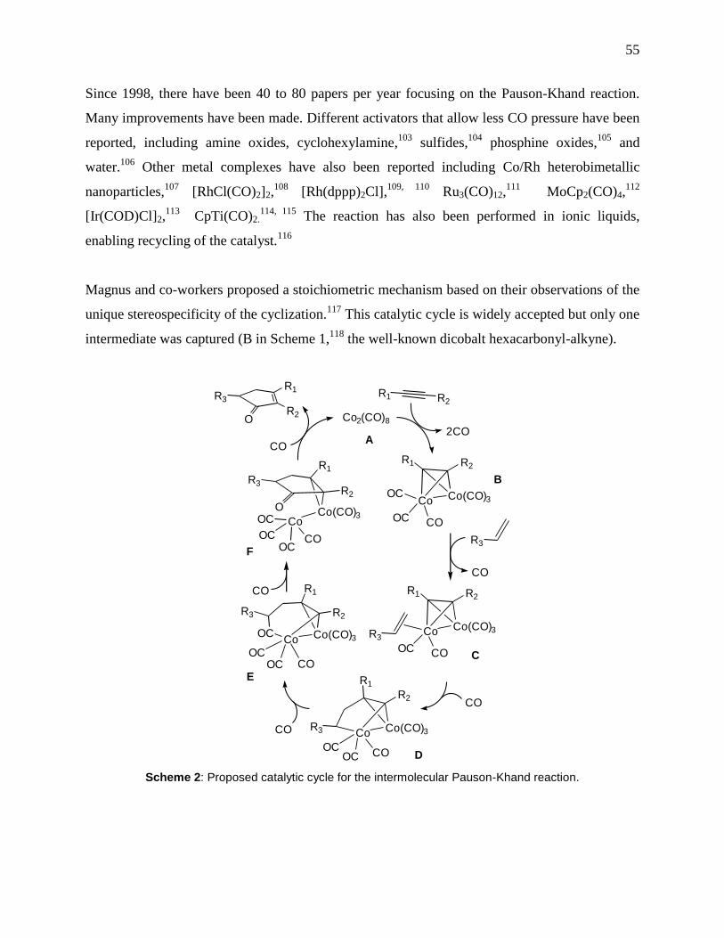
55
Since 1998, there have been 40 to 80 papers per year focusing on the Pauson-Khand reaction.
Many improvements have been made. Different activators that allow less CO pressure have been
reported, including amine oxides, cyclohexylamine,103
sulfides,104
phosphine oxides,105
and
water.106
Other metal complexes have also been reported including Co/Rh heterobimetallic
nanoparticles,107
[RhCl(CO)2]2,108
[Rh(dppp)2Cl],109, 110
Ru3(CO)12,111
MoCp2(CO)4,112
[Ir(COD)Cl]2,113
CpTi(CO)2.114, 115
The reaction has also been performed in ionic liquids,
enabling recycling of the catalyst.116
Magnus and co-workers proposed a stoichiometric mechanism based on their observations of the
unique stereospecificity of the cyclization.117
This catalytic cycle is widely accepted but only one
intermediate was captured (B in Scheme 1,118
the well-known dicobalt hexacarbonyl-alkyne).
Co(CO)3
2CO
Co2(CO)8
Co
R2R1
COOC
OC
Co(CO)3Co
R2R1
COOC
R2R1
R3
Co(CO)3Co
R2
R1
COOC
R3
OC
Co(CO)3Co
R2
R1
OCOC
R3
OC
CO
Co(CO)3Co
R2
R1
OCOC
R3
CO
O
R2
R1R3
O
CO
R3
OC
CO
CO
CO
COA
B
C
D
E
F
Scheme 2: Proposed catalytic cycle for the intermolecular Pauson-Khand reaction.
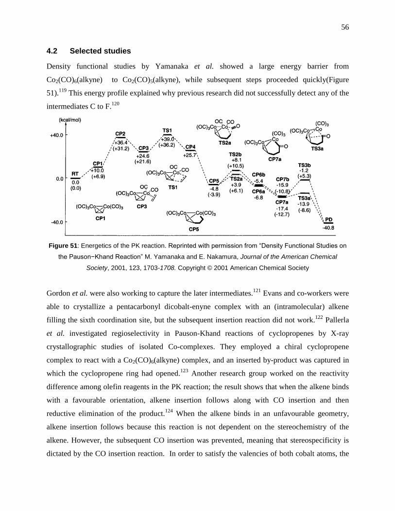
56
4.2 Selected studies
Density functional studies by Yamanaka et al. showed a large energy barrier from
Co2(CO)6(alkyne) to Co2(CO)5(alkyne), while subsequent steps proceeded quickly(Figure
51).119
This energy profile explained why previous research did not successfully detect any of the
intermediates C to F.120
Figure 51: Energetics of the PK reaction. Reprinted with permission from “Density Functional Studies on
the Pauson−Khand Reaction” M. Yamanaka and E. Nakamura, Journal of the American Chemical
Society, 2001, 123, 1703-1708. Copyright © 2001 American Chemical Society
Gordon et al. were also working to capture the later intermediates.121
Evans and co-workers were
able to crystallize a pentacarbonyl dicobalt-enyne complex with an (intramolecular) alkene
filling the sixth coordination site, but the subsequent insertion reaction did not work.122
Pallerla
et al. investigated regioselectivity in Pauson-Khand reactions of cyclopropenes by X-ray
crystallographic studies of isolated Co-complexes. They employed a chiral cyclopropene
complex to react with a Co2(CO)6(alkyne) complex, and an inserted by-product was captured in
which the cyclopropene ring had opened.123
Another research group worked on the reactivity
difference among olefin reagents in the PK reaction; the result shows that when the alkene binds
with a favourable orientation, alkene insertion follows along with CO insertion and then
reductive elimination of the product.124
When the alkene binds in an unfavourable geometry,
alkene insertion follows because this reaction is not dependent on the stereochemistry of the
alkene. However, the subsequent CO insertion was prevented, meaning that stereospecificity is
dictated by the CO insertion reaction. In order to satisfy the valencies of both cobalt atoms, the
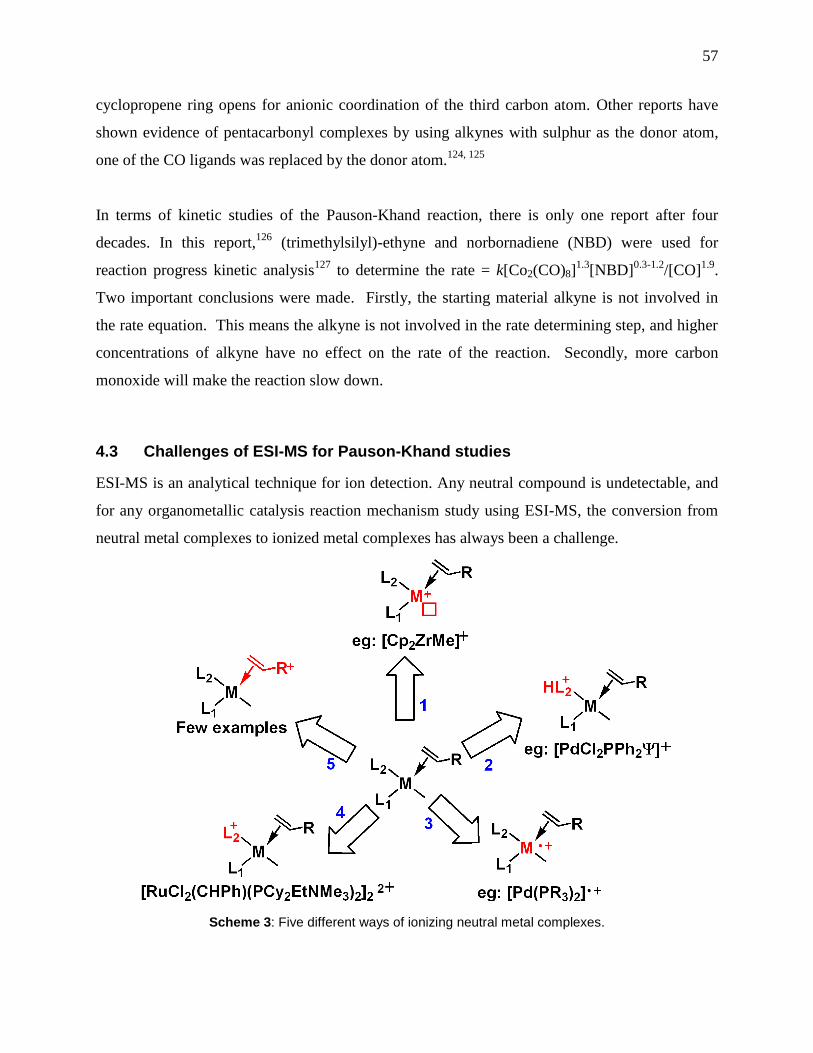
57
cyclopropene ring opens for anionic coordination of the third carbon atom. Other reports have
shown evidence of pentacarbonyl complexes by using alkynes with sulphur as the donor atom,
one of the CO ligands was replaced by the donor atom.124, 125
In terms of kinetic studies of the Pauson-Khand reaction, there is only one report after four
decades. In this report,126
(trimethylsilyl)-ethyne and norbornadiene (NBD) were used for
reaction progress kinetic analysis127
to determine the rate = k[Co2(CO)8]1.3
[NBD]0.3-1.2
/[CO]1.9
.
Two important conclusions were made. Firstly, the starting material alkyne is not involved in
the rate equation. This means the alkyne is not involved in the rate determining step, and higher
concentrations of alkyne have no effect on the rate of the reaction. Secondly, more carbon
monoxide will make the reaction slow down.
4.3 Challenges of ESI-MS for Pauson-Khand studies
ESI-MS is an analytical technique for ion detection. Any neutral compound is undetectable, and
for any organometallic catalysis reaction mechanism study using ESI-MS, the conversion from
neutral metal complexes to ionized metal complexes has always been a challenge.
Scheme 3: Five different ways of ionizing neutral metal complexes.

58
As shown in Scheme 3,128
there are a variety of different ways to charge a neutral metal
complex. (1) loss (or gain) of an anionic ligand such as X– to become an inherently charged
complex;129
(2) a ligand with donor atoms that can form adducts with ions such as H+,130, 131
Na+,132
or Ag+ ;
133 (3) an electron rich oxidizable ligand that can lose an electron in reaction
solution.134
(4) a charged ancillary ligand, most often a phosphine;135
(5) a charged substrate, in
which case the metal complexes can only be detected when the substrate is bound to the
metal.136, 137
In order to use ESI-MS for the study of the Pauson-Khand reaction, the reaction system requires
positive or negative ions in solution phase. The catalyst Co2(CO)8 is a neutral compound and
cannot be detected in mass spectrometry. It has only one ligand that can be ionized, and its
reactivity will be changed if one of the CO ligands is replaced by an ionisable ligand. One of the
substrates, carbon monoxide, is in the gas phase and has no charge, so the alkyne or alkene will
be the only option.
The metal complexes will fall into the fifth category – the charged substrate –as we can syntheze
alkynes or alkenes with a charged tag.
4.4 Advantages of ESI-MS for the Pauson-Khand Reaction studies
There are two advantages in using ESI-MS in the study of this reaction. First, even though
Co2(CO)8 and one of the substrates CO cannot be ionized, the alkyne and alkene functional
group can be easily integrated into a charged tag system. The charged tag can be far away from
the reaction center, so the catalysis reactivity will not be influenced by the ion, and the result will
represent the reaction under real conditions. When the charged alkene and alkyne react with
Co2(CO)8, the intermediates will have a charged tag on them. This allows ESI-MS to detect main
intermediates and short-lived intermediates. Second, a previous study using ESI-MS provided
valuable information and proved this charged tag method is valid. Gimbert and coworkers have
employed a bis(diphenylphosphino)methane (dppm) ligand and a phenylacetylene to make
Co2(CO)4(DPPM)(μ2-HC2C6H5).
138 Under ESI conditions, the dppm ligand deprotonates to
generate a [M-H]– anionic species which is detectable by MS. However, charging the ligand

59
gives only information on the catalyst, not on the overall progress of the reaction. Charging the
substrate does both.
4.5 Results and Discussion
4.5.1 Design of charged substrate
In this project strategy (5) was used to prepare a series of charged pyrrolidinium and
piperidinium salts with alkyne and/or alkene functionality.
Figure 52: Functionalized pyrrolidinium and piperidinium salts. X– = Br
–, PF6
–, BPh4
–, Tf2N
–.
These salts were prepared by me with good yields starting from secondary or tertiary amines.
The synthesis of these salts contains three steps as shown in Scheme 4. In the first step, two
equivalents of secondary amine reacted with one equivalent of 3-bromopropene in a nucleophilic
substitution reaction to generate one equivalent of pyrrolidinium bromide salt and one equivalent
of 1-allylpyrrolidine. This reaction was done in ether at room temperature. The pyrrolidinium
bromide salt by-product was insoluble in ether, so it was easy to filter out. The filtrate was
forwarded to the second step where one equivalent of propargyl bromide was introduced at room
temperature. The bis-functionalized product was insoluble in ether.
After simple filtration, the solid compound was obtained and ready for the next and final step –
the salt metathesis with sodium hexafluorophosphate, sodium tetraphenylborate or sodium
trifluoromethanesulfonimide. All of the metatheses were performed open to the atmosphere in
water.

60
Scheme 4: Synthetic strategy applied to the charged acetylene substrates.
4.5.2 Synthesis of cobalt complexes
In order to obtain detailed structural information of intermediate cobalt complexes, the
synthesized charged salts were introduced to one equivalent of Co2(CO)8 in dichloromethane at
room temperature to form the corresponding Co2(CO)6(μ-alkyne) complex. The synthetic
strategy is exemplified in Scheme 5 for the preparation of [Co2(CO)6(4-3)][PF6]. High quality
ESI-MS spectra were obtained for of [Co2(CO)6(4-3)][PF6] and the rest of the complexes where
the observed peak corresponded to the expected ionic product of Scheme 5.
Scheme 5: Synthetic strategy for ionizing neutral metal complexes.

61
Figure 53: Positive-ion ESI-MS in dichloromethane [Co2(CO)6(4-3)][PF6] (top) and [Co2(CO)6(4-1)][PF6]
(bottom). In both cases, the single peak corresponds to the intact cation.
4-1+ has a single alkyne functional group. As the hexafluorophosphate or tetraphenylborate salt,
it reacted well with Co2(CO)8 to form [Co2(CO)6(4-1)][X], and a single-crystal X-ray structure
was obtained for [Co2(CO)6(4-1)][BPh4] (Figure 54).50

62
Co1Co2
C8
C9
C10
C13N1
C14
O2
O4
O3
O6
O1
O5
C7
Figure 54: Single crystal X-ray structure of the cationic part of [Co2(CO)6(4-1)]+ [BPh4]
–. The
tetraphenylborate anion is not shown for the sake of clarity. Key bond lengths: Co1-Co2 2.461 Å; C7-C8
1.334 Å; C8-C9 1.488 Å; 1.311 0.01 Å; Co-C 1.96 0.01 Å; C-O 1.13 0.01 Å; Co-CO 1.81 0.02 Å;
C-N 1.52 0.02 Å. Key bond angles: C6-C7-C8 146.2°; Co-Co-C 51 1°, Co-C-Co 77.5 0.3°.
4.5.3 Previous gas phase reaction
Previous gas phase studies on probing intermediates, showed [Co2(CO)6(4-1)]+ can undergo an
intermolecular Pauson-Khand reaction in the gas phase with different alkene gases.128
Figure 55: Gas phase reactions of [Co2(CO)6(4-1)]+ with three different alkenes at a cone voltage of 20 V.
In each case, one CO ligand is removed and the alkene adds to [Co2(CO)5(1)]+. The alkene does not add
to the fully saturated ion.

63
The intermediates that were captured in these reactions are [Co2(CO)5(4-1)(alkene)]+. In order to
convert into this species, one CO ligand has to dissociate from the starting material [Co2(CO)6(4-
1)]+. A second conclusion from Figure 55 is that different in bond strains or electronic effects of
alkenes does not influence the reactivity of this coordination process because the results show all
three alkenes have similar reactivity. In other words, alkene coordination is independent of the
subsequent insertion reaction.
The following MS/MS reactions on [Co2(CO)5(4-1)](alkene)+ showed the loss of an alkene as the
first fragment in all three cases. This suggests the alkene is weakly bonded, the bond is weaker
than that of CO to low oxidation state Co, and the insertion is trapped with additional CO.
Therefore, the fact that a complete gas-phase Pauson-Khand transformation could not be
observed was unsurprising, as was the ready loss of alkene upon reactivation using CID.
4.5.4 Intramolecular Pauson-Khand reaction
Charged salts (4-2) and (4-3) have both alkyne and alkene functional groups. This can help to
keep the weakly bonded alkene close to the reaction center to complete the Pauson-Khand
reaction in a simple solution phase analysis.
With the pressurized sample infusion (PSI) online monitoring system, we designed a series of
reactions that were constantly monitored under “real” conditions using ESI-MS. For this
experiment, we used CO as the pressurizing gas. All the chemicals and glassware were initially
protected under N2 and then flushed with CO.
Many experiments were performed before reproducibly good results were obtained. Solubility
differences among starting material, catalyst, by-product and intermediates were the main issues
in these tests. The charged salts have good solubility in polar solvents such as dichloromethane,
methanol, ethanol, acetone, and acetonitrile but they cannot dissolve in nonpolar solvents; the
Co2(CO)8 catalyst can be dissolved easily in apolar solvents such as benzene and toluene, but
many polar solvents will decompose it or replace the CO ligands. All the solvents mentioned
above were tested, and none of them met our experimental requirements.
Fluorobenzene showed better stability for both starting materials and catalyst, and the
intermediates had good solubility in it. Also, fluorobenzene has a high boiling point, enabling
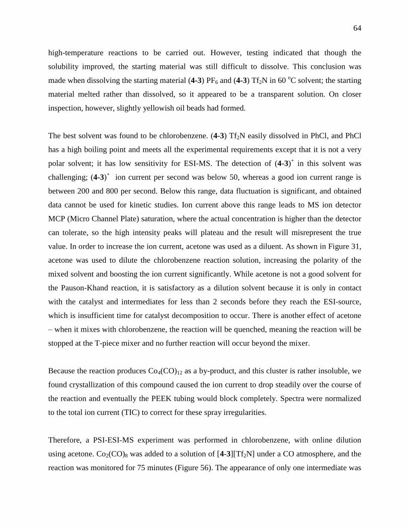
64
high-temperature reactions to be carried out. However, testing indicated that though the
solubility improved, the starting material was still difficult to dissolve. This conclusion was
made when dissolving the starting material (4-3) PF6 and (4-3) Tf2N in 60 oC solvent; the starting
material melted rather than dissolved, so it appeared to be a transparent solution. On closer
inspection, however, slightly yellowish oil beads had formed.
The best solvent was found to be chlorobenzene. (4-3) Tf2N easily dissolved in PhCl, and PhCl
has a high boiling point and meets all the experimental requirements except that it is not a very
polar solvent; it has low sensitivity for ESI-MS. The detection of (4-3)+ in this solvent was
challenging; (4-3)+ ion current per second was below 50, whereas a good ion current range is
between 200 and 800 per second. Below this range, data fluctuation is significant, and obtained
data cannot be used for kinetic studies. Ion current above this range leads to MS ion detector
MCP (Micro Channel Plate) saturation, where the actual concentration is higher than the detector
can tolerate, so the high intensity peaks will plateau and the result will misrepresent the true
value. In order to increase the ion current, acetone was used as a diluent. As shown in Figure 31,
acetone was used to dilute the chlorobenzene reaction solution, increasing the polarity of the
mixed solvent and boosting the ion current significantly. While acetone is not a good solvent for
the Pauson-Khand reaction, it is satisfactory as a dilution solvent because it is only in contact
with the catalyst and intermediates for less than 2 seconds before they reach the ESI-source,
which is insufficient time for catalyst decomposition to occur. There is another effect of acetone
– when it mixes with chlorobenzene, the reaction will be quenched, meaning the reaction will be
stopped at the T-piece mixer and no further reaction will occur beyond the mixer.
Because the reaction produces Co4(CO)12 as a by-product, and this cluster is rather insoluble, we
found crystallization of this compound caused the ion current to drop steadily over the course of
the reaction and eventually the PEEK tubing would block completely. Spectra were normalized
to the total ion current (TIC) to correct for these spray irregularities.
Therefore, a PSI-ESI-MS experiment was performed in chlorobenzene, with online dilution
using acetone. Co2(CO)8 was added to a solution of [4-3][Tf2N] under a CO atmosphere, and the
reaction was monitored for 75 minutes (Figure 56). The appearance of only one intermediate was

65
observed, the expected [Co2(CO)6(4-3)]+. It in turn was consumed, with the appearance of the
product, [4-3 + CO]+. No intermediates were observed in the reaction (i.e. species with more or
less CO ligands than six, collision voltage was also taken into consideration as shown in Figure
57), again consistent with the ligand dissociation step being rate-determining.
Figure 56: Abundance vs. time data for [4-3]+ (starting material), [Co2(CO)6(4-3)]
+ (intermediate) and [4-3
+ CO]+ (product). Data collected using positive ion PSI-ESI-MS in chlorobenzene, online dilution with
acetone, Schlenk flask saturated and pressurized with CO. Data has been normalized to the total ion
current. Scan time of 10 seconds per spectrum. Approximately 20% of the total ion current at the end of
the reaction consisted of numerous low abundance by-products, none of which exceeded 5% of the total.

66
Figure 57: During the PSI-ESI-MS, the collision voltage was set to 2 V. The breakdown graph shows
[Co2(CO)6(4-3)]+ is a stable species at this voltage and it can only be fragmented when the collision
voltage reaches 8 V.
The reaction was repeated at different temperatures, this time starting with the pre-prepared
complex [Co2(CO)6(4-3)][Tf2N], which was injected directly into a hot, CO-saturated solution.
The reaction was conducted at 65.0, 70.0, and 75.0 °C. The temperature was well controlled
within a ± 0.2oC range. Speciation was complicated due to the appearance of aggregates and
solvent adducts, but these signals could be combined to obtain traces of reaction progress (Figure
58). The rate increases with temperature; the first 20% of the reaction is slow, but after that point
each trace follows (pseudo) first-order kinetics. Plotting the natural log of the concentration of
[Co2(CO)8(4-3)]+ vs. time for each experiment produced a plot which was initially curved but
that had a straight line region in the middle (covering conversions from 25% to at least 80% -
reactions were stopped when the total ion current dropped too low to obtain good data), with kobs
= 0.050, 0.099, and 0.245 s-1
at 65, 70, and 75°C respectively.

67
Figure 58: Intensity vs. time data for [Co2(CO)6(4-3)]+ (starting material) and [4-3 + CO]
+ (product),
collected at three different temperatures. Inset: Eyring plot for the three different temperatures.
Enthalpy and entropy of activation were determined using an Eyring plot (Figure 58), which
provided the activation parameters: H‡ = 160 ± 10 kJ mol
-1 and S
‡ = 130 ± 30 J mol
-1 K
-1.
These relatively large values are consistent with the rate-determining step being ligand
dissociation. They compare with values of H‡ = 123.6 ± 11.0 kJ mol
-1 and S
‡ = 72.4 ± 37.3 J
mol-1
K-1
for the rate of reaction of Rh4(CO)12 with an alkyne, another reaction thought to be
limited by dissociation of a CO ligand.139
A positive delta H‡ indicates an endothermic reaction,
and a positive delta S‡ indicates entropy increases. Both of these are consistent with a rate-
determining step of ligand dissociation.
[Co2(CO)6(L)]+ --> [Co2(CO)5(L)]
+ + CO
It is also possible that the species we see as [Co2(CO)6(4-3)]+ actually corresponds to
intermediate D in the cycle (see Scheme 2) because in the intramolecular Pauson-Khand reaction
this species has the same mass as the starting material, intermediate B. This may account for the
initial slower rate of reaction (as it takes time for the process B C D). However, buildup of
D would suggest that the next step, insertion of a CO ligand into a Co-C bond, is slow, and that
this step is unlikely to have a large positive entropy of activation.
68
4.6 Conclusion
The investigations support the prediction that the rate-determining step of the intramolecular
Pauson-Khand reaction is CO dissociation. Gas-phase studies by Matt Henderson on the early
steps in the reaction scheme showed that CO dissociation and alkene coordination can both be
readily achieved, and that the coordination of an alkene is influenced by the nature of the alkene.
This suggests that the effect of the nature of the alkene operates on some later step in the
reaction. Turning to the solution phase, the intramolecular reaction could be monitored using
PSI-ESI-MS, and no intermediates apart from the dicobalt hexacarbonyl ion were observed,
suggesting that the later steps in the reaction are relatively fast. Positive values of H‡ and S
‡
suggest that the rate-determining step is ligand dissociation, consistent with early loss of CO that
allows the alkene to coordinate and the rest of the reaction to proceed.
4.7 Experimental
All solvents were dispensed from an MBraun solvent purification system and used within
minutes. Inert atmosphere techniques were used for all syntheses involving Co2(CO)8. Methyl
pyrrolidine, pyrrolidine, piperidine, allyl bromide, propargyl bromide, sodium
hexafluorophosphate, sodium tetraphenylborate, sodium hydride, sodium chloride, sodium
hydroxide, and dicobalt octacarbonyl were purchased from Aldrich and used without subsequent
purification. NMR spectra were obtained on a Bruker AC 300 spectrometer (1H and 13C).
All mass spectra were collected by using a Micromass Q-TOF micro mass spectrometer in
positive ion mode using pneumatically assisted electrospray ionization: capillary voltage, 2900
V; extraction voltage, 0.5 V; source temperature, 80 °C; desolvation temperature, 150 °C; cone
gas flow, 100 L/h; desolvation gas flow, 100 L/h; collision voltage, 2 V (for MS experiments);
collision voltage, 2–40 V (for MS/MS experiments); low and high mass resolution, 10.0; MCP
voltage, 2700 V. Gas-phase ion–molecule reactions were carried out by a published method.140
4-1 Br. Methyl pyrrolidine (3.8 g, 45.1 mmol) and diethyl ether (30.0 mL) were cooled to 0C in
a 100.0 mL round bottom flask. Propargyl bromide (5.0 mL of an 80% solution in toluene, 6.9 g,
57.5 mmol) in ether (25.0 mL) was added dropwise. The mixture was subsequently allowed to
warm to room temperature and stirred overnight. The solvent was then evaporated and the white
product dried under vacuum for 24 hours. (9.0 g, 44.0 mmol, 97%) M.P.: 62-68C. 1H NMR

69
(CD3OD): (ppm) 4.50 (d, 2H, 3.63Hz); 3.75 (m, 4H); 3.52 (m, 1H); 3.29 (s, 3H); 2.31 (m, 4H).
13C NMR (CD3OD): (ppm) 81.96; 73.33 (f); 65.25; 54.50; 50.44; 23.20.
4-1 PF6. An aqueous solution (20.0 mL H2O) of 1.Br (1.4 g, 7.0 mmol) and sodium
hexafluorophosphate (1.2 g, 7.1 mmol) was prepared. The mixture was heated to facilitate
dissolution, and cooled to room temperature. The white crystals were filtered with a cold water
wash and dried overnight under vacuum. (0.6 g, 2.3 mmol, 33%) M.P.: 146-147C. 1H NMR
(CD3OD): (ppm) 4.33 (d, 2H, 3.63 Hz); 3.67 (m, 4H); 3.45 (m, 1H); 3.22 (s, 3H); 2.28 (m,
4H). 13
C NMR (CD3OD): (ppm) 81.78; 73.05; 65.15; 54.27; 50.24; 23.08. 31
P NMR
(CD3OD): (ppm) -143.22 (septet for PF6–).
Allyl pyrrolidine.141
Allyl bromide (6.0 mL, 8.4 g, 69.4 mmol) in diethyl ether (20.0 mL) was
added dropwise to pyrrolidine (5.1 g, 71.7 mmol) in ether (20.0 mL) at 0C over 30 minutes.
The solution was then allowed to warm to room temperature and stir overnight before
performing a potassium hydroxide extraction (3 × 25.0 mL of a 3.0M solution). The subsequent
aqueous phase was then extracted with dichloromethane and all organic portions were combined,
dried with anhydrous magnesium sulfate, and filtered. The solvent was removed on the rotary
evaporator, and the orange liquid was distilled (fraction that boiled at 120 C was retained) to
give a colorless product. (3.5 g, 31.5 mmol, 45.0 %) 1H NMR (CDCl3): (ppm) 5.88 (m, 1H);
5.21 (m, 2H); 3.02 (d of t, 2H, 6.66Hz, 1.26Hz); 2.43 (m, 4H); 1.71 (m, 4H) 13
C NMR (CDCl3):
(ppm) 136.23, 116.53, 59.22, 53.96, 23.40.
4-2 Br. Allyl pyrrolidine (0.67 g, 6.0 mmol) and propargyl bromide (0.80mL, 1.1 g, 7.2 mmol)
were stirred in ether (30.0 mL) overnight. The white product was filtered and collected (0.45 g,
1.7 mmol, 31.0%). M.P.: 140-146C. 1H NMR (CD3OD): (ppm) 6.11 (m, 1H); 5.76 (m, 2H);
4.30 (s, 2H); 4.16 (d, 2H, 7.29Hz); 3.68 (m, 4H); 3.49 (t, 1H); 2.28 (m, 4H). 13
C NMR
(CD3OD): (ppm) 129.40; 126.55; 82.03; 73.04; 64.55; 63.10; 51.25; 23.22.
4-2 PF6. An aqueous solution of 2.Br (0.27 g, 1.2 mmol, 20.0 mL H2O) was added to an aqueous
solution of sodium hexafluorophosphate (0.21 g, 1.2 mmol, 10.0 mL H2O). The mixture was
70
reduced to a volume of 10.0 mL and left overnight in the fridge at 5 C. The white crystals were
filtered with a water wash and the filtrate was then reduced again to a smaller volume and
transferred back into the fridge for further crystallization. The combined yield of both aliquots
was 0.09 g, 0.31 mmol, 27%. M.P.: 78-80 C. 1H NMR (CD3OD): (ppm) 5.96 (m, 1H); 5.70
(m, 2H); 4.15 (s, 2H); 4.01 (d, 2H, 7.26Hz); 3.55 (m, 4H); 3.36 (t, 1H); 2.16 (m, 4H). 13
C NMR
(CD3OD): (ppm) 129.37; 126.43; 81.96; 72.95; 64.53; 63.03; 51.10; 23.13. 31
P NMR
(CD3OD): (ppm) -143.2 (septet).
Allyl piperidine. Allyl bromide (15.6 g, 128.9 mmol), piperidine (10.5 g, 123.3 mmol), and
sodium hydride (3.3g, 145.9 mmol) were combined as described in the literature to yield allyl
piperidine (11.9 g, 95.0 mmol, 77.0 %) after a partial dynamic vacuum distillation. 1H NMR
(CDCl3): (ppm) 5.82 (m, 1H); 5.05 (m, 2H); 2.89 (d of t, 2H, 6.75Hz, 1.2Hz); 2.30 (s, 4H);
1.52 (m, 4H); 1.37 (m, 2H). 13
C NMR (CDCl3): (ppm) 135.5, 117.33, 62.56, 54.37, 25.86,
24.26.
4-3 Br. Propargyl bromide (2.4 g of 80.0% solution in toluene, 16.2 mmol) in toluene (20.0 mL)
was added to allyl piperidine (1.9 g, 15.5 mmol) in toluene (20.0 mL). The mixture was stirred
at room temperature for 48 hours, and the resulting white product was vacuum filtered, and dried
by vacuum overnight. (2.5 g, 10.1 mmol, 67.0%) M.P.: 154-156C 1H NMR (CD3CN):
(ppm) 5.99-5.70 (m, 3H); 4.43 (s, 2H); 4.15 (d, 2H, 7.32Hz); 3.53 (m, 4H); 3.27 (q, 1H,
1.70Hz); 1.91 (m, 4H); 1.69 (m, 2H). 13
C NMR (CD3CN): (ppm) 129.88; 125.01; 82.68;
71.77; 62.33; 59.23; 50.38; 21.39; 20.31.
4-3 PF6. To 30.0 mL of water was added 3.Br (0.45 g, 1.9 mmol) and sodium
hexafluorophosphate (0.37 g, 2.2 mmol). The mixture was stirred for fifteen minutes and the
white product was filtered (0.22 g). The filtrate was boiled to reduce the volume down to 15.0
mL and transferred to the freezer (-10 C) for four hours. These crystals were then filtered (0.17
g) to give a combined yield of 0.39 g, 1.3 mmol, 68%. M.P.: 85-86C. 1H NMR (CD2Cl2):
(ppm) 5.76 (m, 3H); 3.99 (s, 2H); 3.95 (d, 2H, 7.32Hz); 3.36 (m, 4H); 2.85 (t, 1H); 1.86 (m, 4H);
71
1.70 (q, 2H). 13
C NMR (CD2Cl2): (ppm) 131.46; 122.74; 82.22; 70.17; 62.73; 59.22; 49.45;
20.90; 20.15. 31
P NMR (CD2Cl2): (ppm) -143.82 (septet).
Propargyl piperidine. Piperidine (7.5 mL, 6.5 g, 75.9 mmol) in tetrahydrofuran (50.0 mL) was
added to a slurry of sodium hydride (2.1 g, 85.5 mmol) in tetrahydrofuran (75.0 mL) over 1
hour. The mixture was allowed to stir at room temperature for another hour. A mixture of
propargyl bromide (9.9 g of an 80.0% toluene solution, 66.2 mmol) in tetrahydrofuran was then
added dropwise over an hour and the mixture was left to stir overnight. The mixture was
quenched with a sodium chloride solution (1.0 mol L-1
) and the organic phase separated. The
aqueous phase was then extracted with ethyl acetate (3 × 50.0 mL) followed by tetrahydrofuran
(2 × 50.0 mL) and combined with the original organic fraction. After drying with anhydrous
magnesium sulfate, and filtering with a THF wash, the solvent was removed on a rotary
evaporator and the orange product distilled to give a light yellow liquid (5.4 g, 43.9 mmol,
66.0%). 1H NMR (CDCl3) (ppm): 4.24 (m, 1H); 3.16 (d, 2H, 2.28Hz); 2.39 (m, 4H); 1.51 (m,
4H); 1.34 (m, 2H). 13
C (CDCl3) (ppm): 72.80, 68.36, 52.98, 47.43, 25.73, 23.74.
4-4 Br. Propargyl piperidine (1.0 g, 8.1 mmol) was added to propargyl bromide (1.4 g of an
80.0% toluene solution, 9.2 mmol) along with toluene (30.0 mL) and allowed to stir at room
temperature for 24 hours. The solution was then refluxed for 1 hour, and the brown product was
vacuum filtered with a toluene wash and dried under vacuum overnight. (0.84 g, 3.5 mmol, 43.0
%) M.P.: 200 C (dec.). 1H NMR (CD3OD): (ppm) 4.50 (d, 4H, 2.37Hz); 3.62 (t, 4H,
5.67Hz); 3.55 (t, 2H, 2.49Hz); 1.95(m, 4H); 1.72(m, 2H). 13
C (CD3CN): (ppm) 83.00; 71.09;
59.45; 51.01; 21.19; 20.29.
4-4 PF6. As for 1.PF6 with the following amounts of reagents and solvents: 4.Br (0.17 g, 0.69
mmol), sodium hexafluorophosphate (0.18 g, 1.1 mmol), water (30.0 mL), isolated product
(0.080 g, 0.26 mmol, 38.0 %). M.P.: 160-161. 1H NMR (CD3OD): (ppm) 4.46 (s, 4H); 3.62
(t, 4H, 5.73Hz); 3.53 (t, 2H, 3.27Hz); 1.97 (m, 4H); 1.74 (m, 2H). 13
C NMR (CD3OD): (ppm)
83.39; 71.33; 59.90; 51.05; 21.81; 20.68. 31
P (CD3OD): (ppm) -143.24 (septet).
[Co2(CO)6(4-3)][PF6]. Dicobalt octacarbonyl (0.15 g, 0.44 mmol) and 3b (0.087 g, 0.28 mmol)
were added to a Schlenk flask as solids against a dry nitrogen atmosphere. Dry dichloromethane

72
(10.0 mL) was then added and the mixture was allowed to react for two hours. The solvent was
then evaporated, and the red solid was washed with ether (3 x 8.0 mL) and then dried under
vacuum for 2 hours. The dark red product (0.13 g, 0.22 mmol, 78.0%) was collected and X-ray
quality crystals were grown by dichloromethane and ether solvent diffusion in the freezer, with a
small layer of 1-butanol between them. M.P. 90 C (dec.). 1H NMR (CD2Cl2): (ppm) 6.38 (s,
1H); 5.74 (m, 3H); 4.70 (s, 2H); 4.00 (d, 2H); 3.42 (m, 4H); 1.88 (m, 4H); 1.72 (m, 2H). 13
C
NMR (CD2Cl2): (ppm) 130.91, 122.91, 75.25, 74.03, 62.69, 62.10, 58.86, 20.96, 20.32. 31
P
NMR (CD2Cl2) (ppm) -143.79 (septet). IR (cm-1
, CH2Cl2): 2105 (st), 2066 (vs), 2045 (vs).
UV-Vis: 356 nm, 364 nm, 421 nm.
Table 3: Aggregates and species in the reaction solution:
Species Mass
C8H16N
125.5
3+ C11H18N
164.2
Product C12H18NO
192.1

73
+ + C12H18NO C8H16N C2F6NO4S2
598.2
+ + C12H18NO x 2 + C2F6NO4S2
664.2
+ + + C11H18N + C8H16N+ C2F6NO4S2 + Co2(CO)6
856.0
+ + + C11H18N x2 + Co2(CO)6 + C2F6NO4S2
894.1
+ + + C11H18N + Co2(CO)6 + C12H18NO + C2F6NO4S2
922.1

74
+ + + + C11H18N x2 + Co2(CO)6 x2 + C2F6NO4S2
1180.1
75
5. Detailed kinetic analysis of rhodium-catalyzed alkyne
hydrogenation
Portions of this chapter have been previously published, and are reproduced in part with
permission from “A detailed kinetic analysis of rhodium-catalyzed alkyne hydrogenation” J.
Luo, A. G. Oliver and J. Scott McIndoe, Dalton Transactions, 2013, 42, 11312-11318. Copyright
© The Royal Society of Chemistry 2013
I performed all experimental work, produced all figures and co-wrote the paper with JS
McIndoe. AG Oliver performed the crystal structure determinations. The wilkinson’s
hydrogenation part was published, the Weller’s hydrogenation part is in preparation.
Hydrogenation of alkynes and alkenes mediated by rhodium complexes is a classic catalytic
organometallic reaction.142
The mechanism of these reactions has been studied extensively by
different methods. In this chapter, a variety of hydrogenation reactions were performed and
analyzed using PSI-ESI-MS.
5.1 Hydrogenation of olefins by Rh (PPh3)3Cl
5.1.1 Introduction
Homogeneous hydrogenation of olefins was first introduced by Wilkinson.143
Since the reports
of the now well-known catalyst Rh(PPh3)3Cl in 1965,143-145
Wilkinson and others have studied its
catalytic capabilities in the hydrogenation of unsaturated substrates. Since then, this catalyst has
been widely used due to its high efficiency and high sensitivity as well its ability to function
under virtually unrestricted conditions. It has become one of the most famous catalysts in the
world, and is known as “Wilkinson’s catalyst”.
The mechanism of the reaction has been studied by a wide range of different methods and it has
become the most well-understood organometallic catalytic reaction. Every step of the catalytic
cycle has been reported. Halpern et al. reported a detailed kinetic study and investigated the
76
mechanism of oxidative addition of Rh(PPh3)3Cl with H2 and cyclohexene. NMR and UV/Vis
spectroscopy were used for acquiring experimental data, and a number of rate constants were
obtained. The authors also indicated the rate determining step involved Rh-H bond breakage by
measuring kinetic isotope effect through replacing RhH2(PPh3)3Clwith RhD2(PPh3)3Cl.146
In a
recent study, Cabrera and co-workers used experimental data to build kinetic models of this
hydrogenation by using avermectins B1a and B1b as substrates and Rh(PPh3)3Cl as catalyst. The
kinetic model includes a proposed catalytic cycle and all the rate constants of all the steps of the
reaction.147
In another study, the electronic and steric effects on nucleophilic addition to the alkene double
bond were investigated to help reveal the reasons behind the selectivity towards different types
of π bonds during the hydrogenation reaction.148
Bowker et al. used temperature programmed desorption to compare homogeneous Wilkinson’s
hydrogenation with heterogeneous hydrogenation on compound Rh(III). They concluded that the
homogeneous and heterogeneous hydrogenation mechanisms have certain similarities.149
Koga et al. reported the first energy profile study of the whole catalytic cycle of Wilkinson’s
hydrogenation in 1986.150
Wink and Ford performed a flash photolysis investigation on the key
intermediate Rh(PPh3)2Cl and its reaction with CO, C2H4,PPh3 and H2; various important
equilibrium constants were acquired.151, 152
Para-hydrogen induced polarisation NMR techniques
provided important information on probing previously unobserved intermediates, especially
dihydride species in the dynamic reaction system.153-155
All the techniques that were mentioned above, when combined together gave us a clear picture of
the Wilkinson’s hydrogenation catalytic cycle. The generally accepted main cycle is shown in
Scheme 6. 156
The PPh3 ligand dissociation to generate intermediate Rh(PPh3)2Cl is the first step
of catalysis. The intermediate with a vacant site is more reactive, it is ready to undergo oxidative
addition with H2 followed by ligand association of the olefin. After 1,2 insertion of the olefin,
there is a reductive elimination to finish the catalytic cycle. The product alkane is released to the
medium and the catalyst is converted back into the Rh(PPh3)2Cl species.
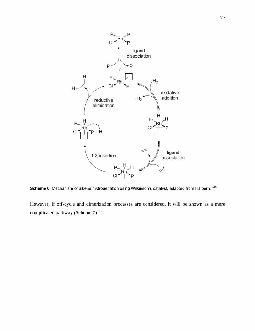
77
Scheme 6: Mechanism of alkene hydrogenation using Wilkinson’s catalyst, adapted from Halpern. 156
However, if off-cycle and dimerization processes are considered, it will be shown as a more
complicated pathway (Scheme 7).135
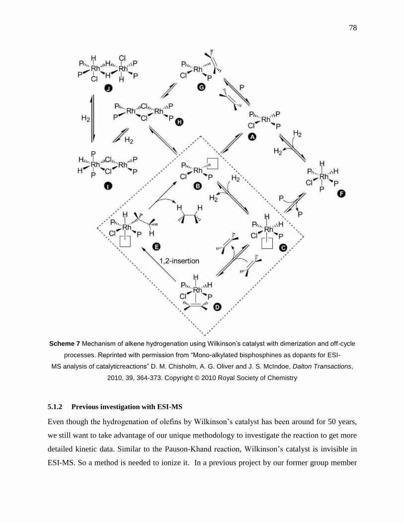
78
Scheme 7 Mechanism of alkene hydrogenation using Wilkinson’s catalyst with dimerization and off-cycle
processes. Reprinted with permission from “Mono-alkylated bisphosphines as dopants for ESI-
MS analysis of catalyticreactions” D. M. Chisholm, A. G. Oliver and J. S. McIndoe, Dalton Transactions,
2010, 39, 364-373. Copyright © 2010 Royal Society of Chemistry
5.1.2 Previous investigation with ESI-MS
Even though the hydrogenation of olefins by Wilkinson’s catalyst has been around for 50 years,
we still want to take advantage of our unique methodology to investigate the reaction to get more
detailed kinetic data. Similar to the Pauson-Khand reaction, Wilkinson’s catalyst is invisible in
ESI-MS. So a method is needed to ionize it. In a previous project by our former group member

79
Dr. Danielle Chisholm, sub-stoichiometric quantities of a charged phosphine ligand
[Ph2P(CH2)4PPh2Bn]+ [PF6]
– were added into the reaction.
157 The introduction of this charged
phosphine ligand substituted one of the PPh3 ligands to generate a charged version of
Wilkinson’s catalyst (Equation 3). Hydrogenation was performed in chlorobenzene, and various
rhodium complexes were observed consistent with the known speciation of this reaction
mixture(Figure 59).135
Equation 3
Figure 59: Positive ions of ionized Wilkinson’s catalyst, where 5-1+ is [Ph2P(CH2)4PPh2Bn]
+. Reprinted
with permission from “Mono-alkylated bisphosphines as dopants for ESI-MS analysis of catalytic
reactions” D. M. Chisholm, A. G. Oliver and J. S. McIndoe, Dalton Transactions, 2010, 39, 364-373.
Copyright © 2010 Royal Society of Chemistry
However, because ESI-MS operates only on ions, only catalyst-containing species are observed,
so the overall progress of the reaction was not tracked and therefore the concentration of
intermediates cannot be matched to activity. It is unable to decide if the observed species are
truly reactive intermediates, resting states or decomposition products. Although the system can

80
be combined with other techniques to get correlated data, the methodology should be modified to
make it an independent standalone analysis technique to measure intermediates and track
reaction progress. Based on the Pauson-Khand reaction, we have found that if the substrate is
charged, we can achieve this goal. So here we have used a charge-tagged alkyne to enable us to
track the progress of the reaction as well as detect any appreciable quantities of intermediates
that include the charged tag.
5.1.3 Results and Discussion
5.1.3.1 Design of charged substrate
There are many strategies to integrate a charged tag with an alkyne. For an ideal charged alkyne
that has conveyed amenability for ESI-MS analysis, it must meet the following requirements: 1)
the charged tag itself should not be involved in the reaction or influence reactivity of the catalyst
or the alkyne or any other functional groups; 2) it should be easy to prepare, ideally, the
synthesis route should be under four steps, the less the better. Even though the reaction only
takes a very small quantity of the substrate, it has to be simple. It should represent a widely used
olefin substrate in other Wilkinson’s hydrogenation research; 3) it should be easy to purify, and
the purity has to be high after purification, so the final product should be a single peak in ESI-
MS spectrum; 4) It should be high in mass (higher than m/z 200) and have high surface activity,
so it will dominate spectral intensity and providing very similar response factors for all ions
involving that tag; 5) It should have a relatively non-coordinating anion, to maximally reduce the
extent of ion pairing, improving sensitivity and minimizing the appearance of complicating
aggregate ions.
Initially, a triphenylphosphonium salt in which the alkyne was remote from the charge,
[Ph3P(CH2)(C6H4)C2H]+[PF6]
– (5-2), was tried (Scheme 8). The synthesis is straightforward, in
order to get pure product, we chose to convert the starting material into charged salt in the first
step. The second step is a Sonogashira coupling reaction with CuI as co-catalyst. In the third
step, K2CO3 was used to remove TMS, however, the reaction time must be controlled accurately,
in our case, the reaction took 70 minutes. Over 70 minutes, the dimerized byproduct will form
and we found if this happens, the following purification step is very hard. The reaction was
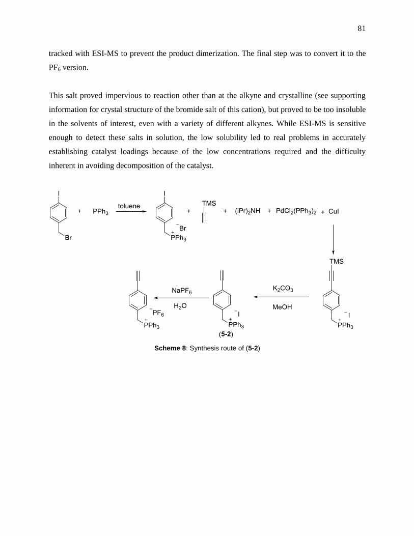
81
tracked with ESI-MS to prevent the product dimerization. The final step was to convert it to the
PF6 version.
This salt proved impervious to reaction other than at the alkyne and crystalline (see supporting
information for crystal structure of the bromide salt of this cation), but proved to be too insoluble
in the solvents of interest, even with a variety of different alkynes. While ESI-MS is sensitive
enough to detect these salts in solution, the low solubility led to real problems in accurately
establishing catalyst loadings because of the low concentrations required and the difficulty
inherent in avoiding decomposition of the catalyst.
Scheme 8: Synthesis route of (5-2)
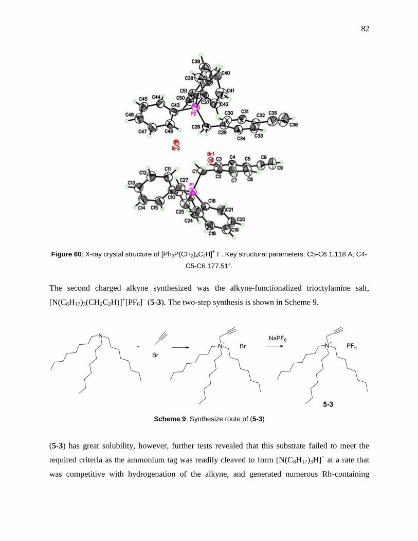
82
Figure 60: X-ray crystal structure of [Ph3P(CH2)4C2H]+ I
–. Key structural parameters: C5-C6 1.118 A; C4-
C5-C6 177.51°.
The second charged alkyne synthesized was the alkyne-functionalized trioctylamine salt,
[N(C8H17)3(CH2C2H)]+[PF6]
– (5-3). The two-step synthesis is shown in Scheme 9.
Scheme 9: Synthesize route of (5-3)
(5-3) has great solubility, however, further tests revealed that this substrate failed to meet the
required criteria as the ammonium tag was readily cleaved to form [N(C8H17)3H]+ at a rate that
was competitive with hydrogenation of the alkyne, and generated numerous Rh-containing

83
catalyst decomposition products. 5-3 also produced significant amounts of aggregates of the
form [(cation)n + (anion)n-1]+,158
making the analysis complicated.
Another charged alkyne [Ph3P(CH2)4C2H]+[PF6]
– (5-4) was readily prepared from 6-
bromohexyne and triphenylphosphine, followed by salt metathesis with Na[PF6].
Scheme 10: Synthesis route of (5-4)
5-4 had no problems related to solubility, reactivity or aggregation as the [PF6]– salt, and all
experiments described used this phosphonium-tagged terminal alkyne as the substrate.
Crystals of [Ph3P(CH2)4C2H]+I– (the alkyne starting material, before metathesis of the iodide salt
for [PF6]– to make 5-4) were obtained and used to acquire an X-ray crystal structure (Figure 61).
Structural parameters are entirely ordinary, in keeping with the idea that there is nothing
exceptional about the alkyne functional group - it is remote enough from the charged tag that its
chemistry is unaffected by the distant modification.
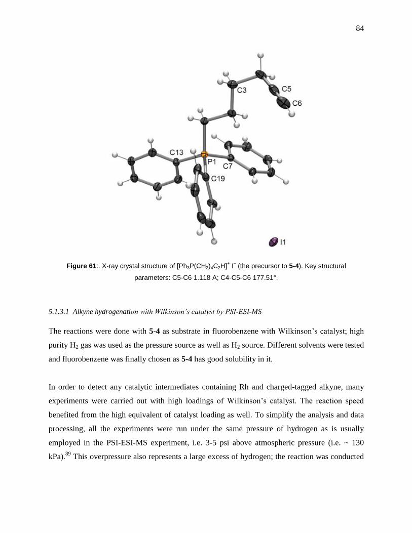
84
Figure 61:. X-ray crystal structure of [Ph3P(CH2)4C2H]+ I
– (the precursor to 5-4). Key structural
parameters: C5-C6 1.118 A; C4-C5-C6 177.51°.
5.1.3.1 Alkyne hydrogenation with Wilkinson’s catalyst by PSI-ESI-MS
The reactions were done with 5-4 as substrate in fluorobenzene with Wilkinson’s catalyst; high
purity H2 gas was used as the pressure source as well as H2 source. Different solvents were tested
and fluorobenzene was finally chosen as 5-4 has good solubility in it.
In order to detect any catalytic intermediates containing Rh and charged-tagged alkyne, many
experiments were carried out with high loadings of Wilkinson’s catalyst. The reaction speed
benefited from the high equivalent of catalyst loading as well. To simplify the analysis and data
processing, all the experiments were run under the same pressure of hydrogen as is usually
employed in the PSI-ESI-MS experiment, i.e. 3-5 psi above atmospheric pressure (i.e. ~ 130
kPa).89
This overpressure also represents a large excess of hydrogen; the reaction was conducted
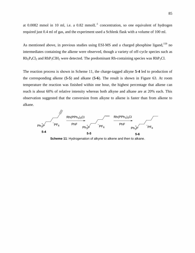
85
at 0.0082 mmol in 10 ml, i.e. a 0.82 mmolL-1
concentration, so one equivalent of hydrogen
required just 0.4 ml of gas, and the experiment used a Schlenk flask with a volume of 100 ml.
As mentioned above, in previous studies using ESI-MS and a charged phosphine ligand,159
no
intermediates containing the alkene were observed, though a variety of off-cycle species such as
Rh2P4Cl2 and RhP3ClH2 were detected. The predominant Rh-containing species was RhP3Cl.
The reaction process is shown in Scheme 11, the charge-tagged alkyne 5-4 led to production of
the corresponding alkene (5-5) and alkane (5-6). The result is shown in Figure 63. At room
temperature the reaction was finished within one hour, the highest percentage that alkene can
reach is about 60% of relative intensity whereas both alkyne and alkane are at 20% each. This
observation suggested that the conversion from alkyne to alkene is faster than from alkene to
alkane.
Scheme 11: Hydrogenation of alkyne to alkene and then to alkane.

86
Figure 62: Positive-ion ESI-MS in fluorobenzene, [PPh3P(CH2)4CCH]PF6 (bottom) is the starting material.
[PPh3P(CH2)5CH3]PF6 (top) is the final product.
Figure 63 Relative intensity vs time traces for alkyne (5-4), alkene (5-5) and alkane (5-6).
This reaction was run at room temperature with a high catalyst loading to maximize the chances
of observing a rhodium-containing intermediate that included the charged tag, different cone

87
voltages were tested as well as cone gas flow rate and other ESI and TOF parameters. But no
such intermediates were observed. The results are similar to a previous ESI study. This negative
result tells us that the 1,2-insertion and the reductive elimination are not turnover limiting steps
as we would expect the intermediates prior to each of these steps should have a fairly high and
detectable intensity. It does not tell us whether the phosphine dissociation, oxidative addition of
dihydrogen, or alkyne/alkene binding are turnover-limiting steps, because the tagged ligand is
not involved in any of these steps.
The experiment was conducted at different temperatures in order to exclude the possibility that
the reactivity observed is some sort of fact of the electrospray process itself or a gas-phase
phenomenon. Cooks noted that certain reactions are greatly accelerated during supersonic
expansion in the ESI process (by several orders of magnitude in one example).160
However, if
that were the case in these reactions, we would expect to see similar reactivity regardless of the
reaction flask temperature. However, this is not the case; the reaction is very fast at high flask
temperatures, and very slow at cold flask temperatures, and both were collected under ESI source
conditions that were identical. This observation is strong evidence for the data representing
solution rather than gas-phase conditions. The three temperatures examined were 0.0 °C, 23.0 °C
(ambient) and 58.2 °C. The temperature of the solution was not controlled when it goes through
the PEEK tubing between flask and ESI source, so in each case, there was a brief period (on the
order of a few seconds) in which the reaction temperature was altered.
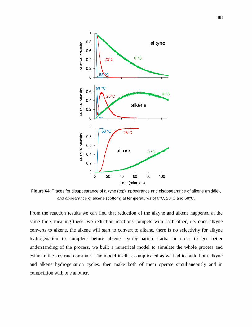
88
Figure 64: Traces for disappearance of alkyne (top), appearance and disappearance of alkene (middle),
and appearance of alkane (bottom) at temperatures of 0°C, 23°C and 58°C.
From the reaction results we can find that reduction of the alkyne and alkene happened at the
same time, meaning these two reduction reactions compete with each other, i.e. once alkyne
converts to alkene, the alkene will start to convert to alkane, there is no selectivity for alkyne
hydrogenation to complete before alkene hydrogenation starts. In order to get better
understanding of the process, we built a numerical model to simulate the whole process and
estimate the key rate constants. The model itself is complicated as we had to build both alkyne
and alkene hydrogenation cycles, then make both of them operate simultaneously and in
competition with one another.

89
Figure 65: Catalytic cycle for hydrogenation of alkyne to alkane, where the two hydrogenations compete
with one another.
The program PowerSim 161
was used to model each of the steps and published references were
consulted to find rate constants as a starting point for as many steps as possible.146, 162, 163
For all
the other parameters, manual adjustment was done. Manual adjustments were time consuming,
and later on with the acquisition of COPASI, models could be constructed in much less time. For
the reaction at 23 °C and 17% catalyst loading, the modelled rates that provided the best match
with experimental data are listed in Table 4. During the estimation process, the large number of
independent parameters have to be tested and the numbers need to be treated with some
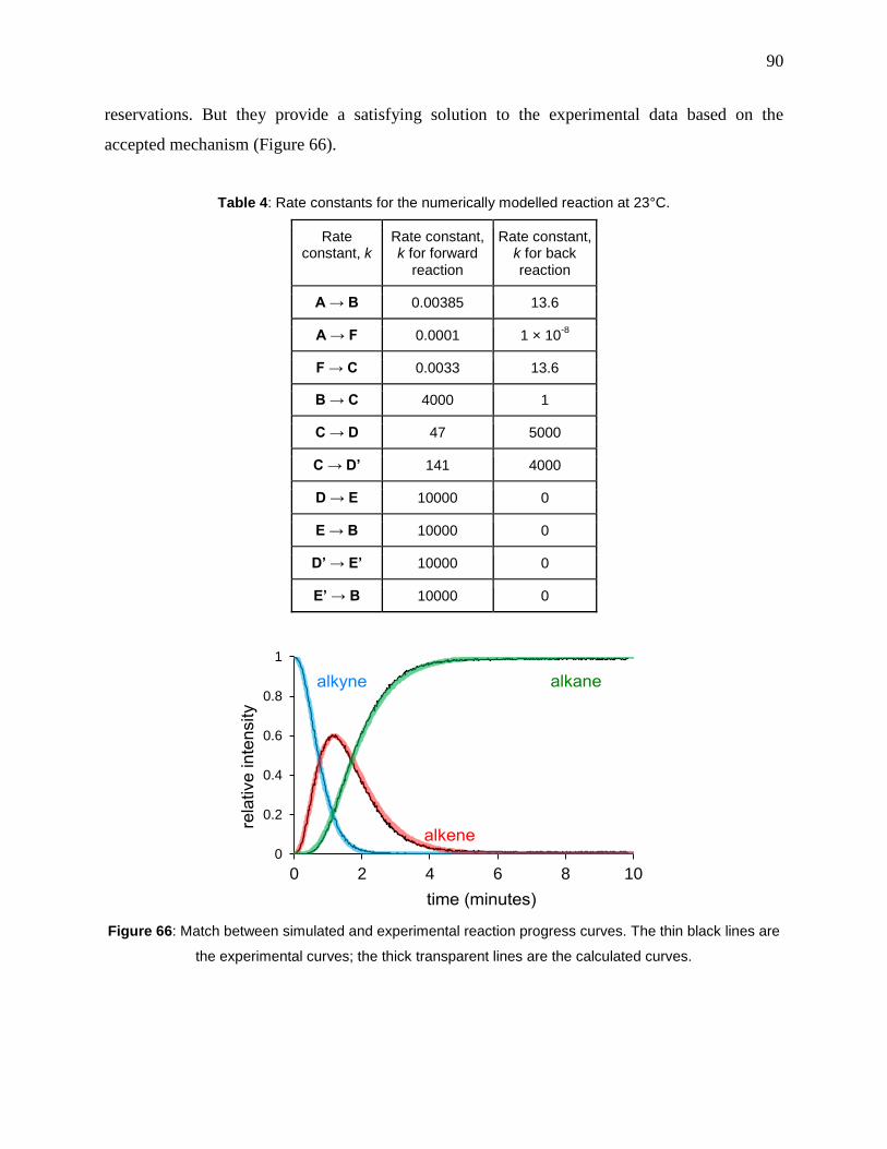
90
reservations. But they provide a satisfying solution to the experimental data based on the
accepted mechanism (Figure 66).
Table 4: Rate constants for the numerically modelled reaction at 23°C.
Rate constant, k
Rate constant, k for forward
reaction
Rate constant, k for back reaction
A → B 0.00385 13.6
A → F 0.0001 1 × 10⁻⁸
F → C 0.0033 13.6
B → C 4000 1
C → D 47 5000
C → D’ 141 4000
D → E 10000 0
E → B 10000 0
D’ → E’ 10000 0
E’ → B 10000 0
0
0.2
0.4
0.6
0.8
1
0 2 4 6 8 10
Figure 66: Match between simulated and experimental reaction progress curves. The thin black lines are
the experimental curves; the thick transparent lines are the calculated curves.
91
From the estimated parameter we can find out that the initial ligand dissociation from A to B is
slow as the rate constant for the back reaction is much larger than the forward reaction. To match
accurately to the rest of the reaction, the final steps of the reaction proved to be fast (modelled as
irreversible reactions with rates of 10000 units, but the model is essentially insensitive to
changes in these rates once they are faster than the earlier reactions in the cycle). The slowest
steps of the productive part of the cycle are ligand association of alkene or alkyne with the
unsaturated 16e RhIII
complex, P2Rh(H)2Cl, C. That a ligand association should be slow is
somewhat counterintuitive unless the fact that a solvent molecule needs to be displaced first is
taken into account (solvent involvement was not explicitly modelled). The model predicts that
the ligand association reaction lies a long way towards the unsaturated (= solvent coordinated)
complex, and that the forward reaction is approximately three times faster for the alkyne over the
alkene (the back reactions are much faster and both of similar magnitude). This low level of
selectivity means that partial hydrogenation164-167
is not feasible with Wilkinson’s catalyst, at
least without the addition of modifying agents.168
Because the key rate constant is the ligand dissociation step to generate the unsaturated 14
electron RhP2Cl from RhP3Cl, we would expect the reaction to be inhibited by the addition of
PPh3 (the mechanism predicts a reaction rate that is inversely first order in triphenylphosphine
concentration). That proves to be true; the reaction slows substantially with added PPh3. The
experiments were conducted with 5% catalyst at 91.0 °C, in order to expedite the analyses. Extra
PPh3 was loaded before the catalyst solution was added, with 0 eq, 1 eq to catalyst and 2 eq to
catalyst. The changes in reaction rate were predicted well by our numerical model when we
altered only the initial concentration of PPh3 (Figure 67), adding confidence to its accuracy.
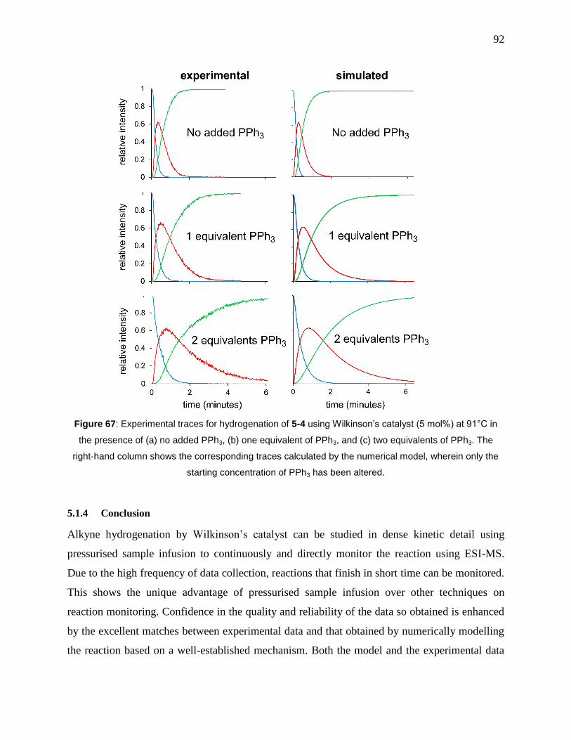
92
Figure 67: Experimental traces for hydrogenation of 5-4 using Wilkinson’s catalyst (5 mol%) at 91°C in
the presence of (a) no added PPh3, (b) one equivalent of PPh3, and (c) two equivalents of PPh3. The
right-hand column shows the corresponding traces calculated by the numerical model, wherein only the
starting concentration of PPh3 has been altered.
5.1.4 Conclusion
Alkyne hydrogenation by Wilkinson’s catalyst can be studied in dense kinetic detail using
pressurised sample infusion to continuously and directly monitor the reaction using ESI-MS.
Due to the high frequency of data collection, reactions that finish in short time can be monitored.
This shows the unique advantage of pressurised sample infusion over other techniques on
reaction monitoring. Confidence in the quality and reliability of the data so obtained is enhanced
by the excellent matches between experimental data and that obtained by numerically modelling
the reaction based on a well-established mechanism. Both the model and the experimental data

93
responded in the same way to perturbations to the concentration of free phosphine, which
predictably slows the reaction given that the turnover-limiting step involves dissociation of the
phosphine from Wilkinson’s catalyst to generate the unsaturated, 14-electron complex that
rapidly oxidatively adds hydrogen.
5.2 Hydrogenation of olefins by Weller’s catalyst
5.2.1 Introduction
In the first part of the chapter, Wilkinson’s catalyst was used for the study of alkyne
hydrogenation where it was confirmed that the turnover-limiting step was ligand dissociation
from the precatalyst to generate the unsaturated, 14-electron species Rh(PPh3)2Cl. We also used
the charged alkyne to make the whole reaction detectable in mass spectrometry; however, we
saw no metal-containing intermediates during the reaction. We went looking for a charged
catalyst that would perform the same transformation, and decided on a cationic rhodium
complex. A cationic rhodium complex will give us a chance to detect any charged Rh peak in
MS. These are well known to be excellent selective hydrogenators of alkynes, from the classic
work of Schrock and Osborn from the 1970s.169
Finally the cationic catalyst,
[Rh(PCpr3)2(PhF)]+[B[3,5-(CF3)2C6H3]4]
– (P
Cpr3 = triscyclopropylphosphine, PhF =
fluorobenzene) was chosen.170
Because the catalyst was firstly synthesized and provided by
Professor Andrew Weller from University of Oxford, here we call this catalyst, “Weller’s
catalyst”.
Cationic rhodium complexes of the type [Rh(diene)(PR3)2]PF6 are known for hydrogenation of
alkynes from Schrock and Osborn’s work,169
and since then these type of complexes have
served as precursors in various studies of homogeneous catalysis. Bis(ditertiaryphosphine)
chelate complexes of rhodium(I) were studied as catalytic hydrogenators of methylene succinic
acid, and cationic and hydrido versions of the complex were found to be more active than
corresponding chloro versions with activity increasing with increasing chain length of the
diphosphine.171
Additionally the complex [Rh(NBD)(PPh3)2][BF4] (NBD = 2,5-norbornadiene)
was found to selectively catalyze phenylacetylene to styrene without reduction of the diolefin of
the catalyst, proof that the active species is diolefin coordinated instead of dihydrido and
monohydrido derivatives.172
Semihydrogenation of internal alkenes such as diphenylacetylene
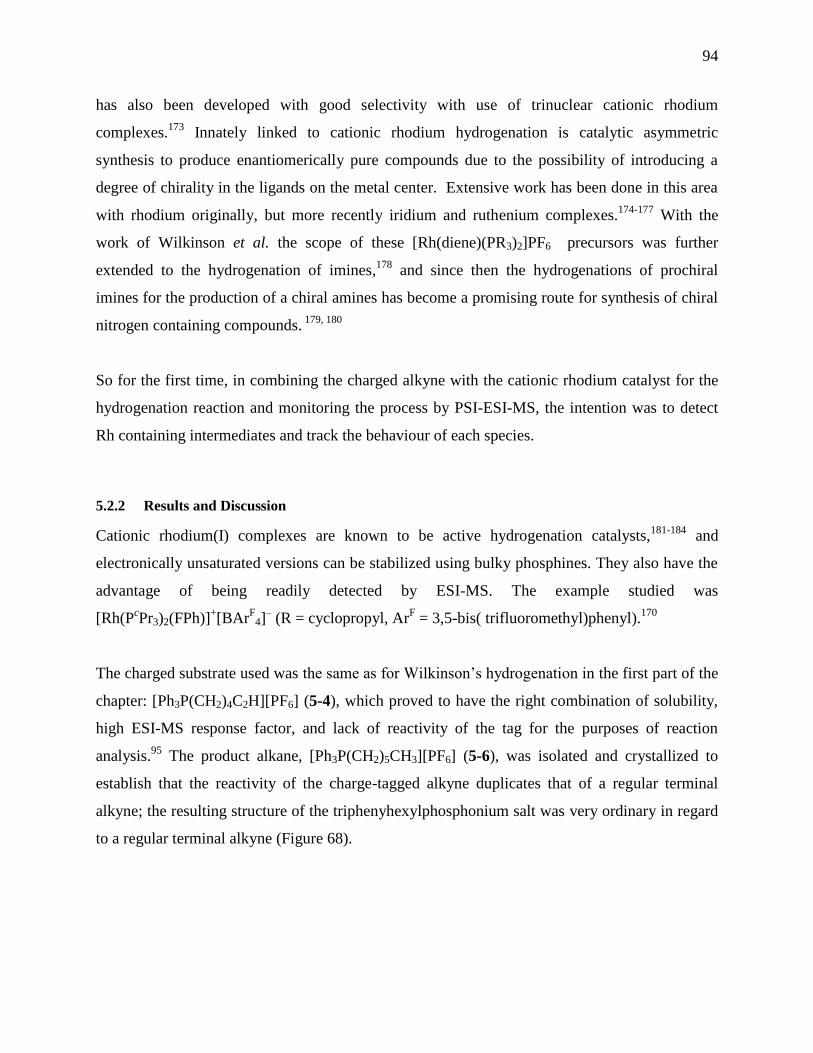
94
has also been developed with good selectivity with use of trinuclear cationic rhodium
complexes.173
Innately linked to cationic rhodium hydrogenation is catalytic asymmetric
synthesis to produce enantiomerically pure compounds due to the possibility of introducing a
degree of chirality in the ligands on the metal center. Extensive work has been done in this area
with rhodium originally, but more recently iridium and ruthenium complexes.174-177
With the
work of Wilkinson et al. the scope of these [Rh(diene)(PR3)2]PF6 precursors was further
extended to the hydrogenation of imines,178
and since then the hydrogenations of prochiral
imines for the production of a chiral amines has become a promising route for synthesis of chiral
nitrogen containing compounds. 179, 180
So for the first time, in combining the charged alkyne with the cationic rhodium catalyst for the
hydrogenation reaction and monitoring the process by PSI-ESI-MS, the intention was to detect
Rh containing intermediates and track the behaviour of each species.
5.2.2 Results and Discussion
Cationic rhodium(I) complexes are known to be active hydrogenation catalysts,181-184
and
electronically unsaturated versions can be stabilized using bulky phosphines. They also have the
advantage of being readily detected by ESI-MS. The example studied was
[Rh(PcPr3)2(FPh)]
+[BAr
F4]
– (R = cyclopropyl, Ar
F = 3,5-bis( trifluoromethyl)phenyl).
170
The charged substrate used was the same as for Wilkinson’s hydrogenation in the first part of the
chapter: [Ph3P(CH2)4C2H][PF6] (5-4), which proved to have the right combination of solubility,
high ESI-MS response factor, and lack of reactivity of the tag for the purposes of reaction
analysis.95
The product alkane, [Ph3P(CH2)5CH3][PF6] (5-6), was isolated and crystallized to
establish that the reactivity of the charge-tagged alkyne duplicates that of a regular terminal
alkyne; the resulting structure of the triphenyhexylphosphonium salt was very ordinary in regard
to a regular terminal alkyne (Figure 68).
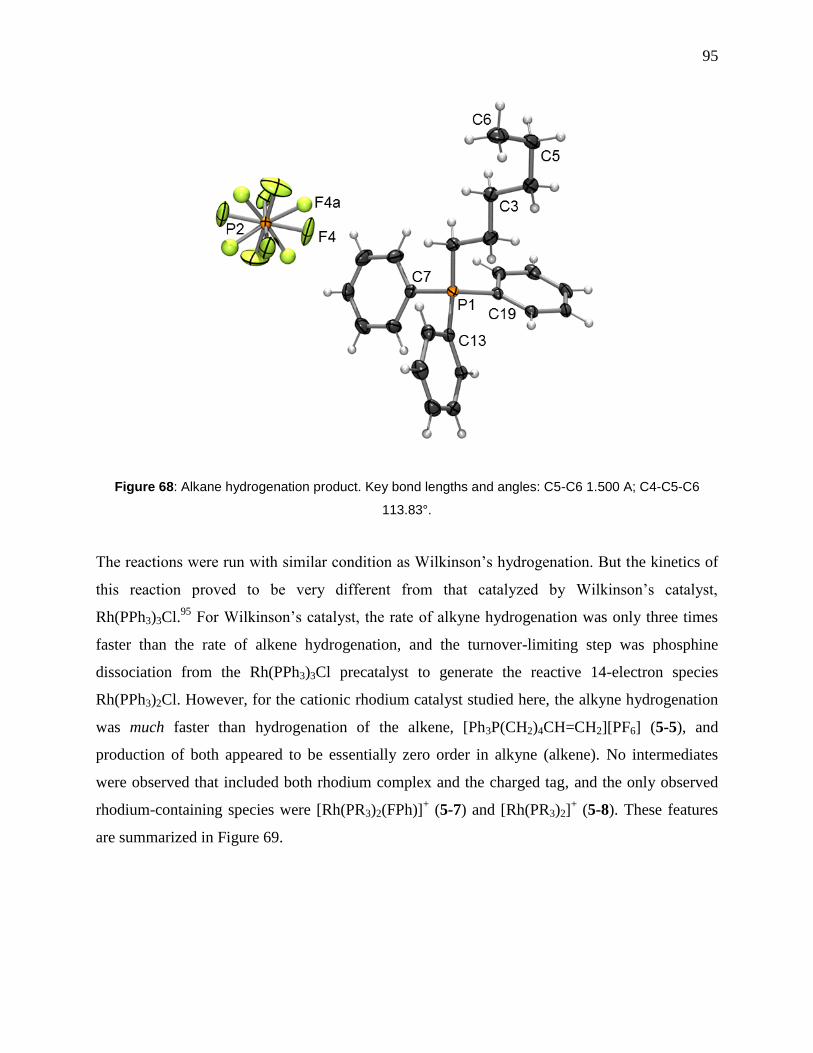
95
Figure 68: Alkane hydrogenation product. Key bond lengths and angles: C5-C6 1.500 A; C4-C5-C6
113.83°.
The reactions were run with similar condition as Wilkinson’s hydrogenation. But the kinetics of
this reaction proved to be very different from that catalyzed by Wilkinson’s catalyst,
Rh(PPh3)3Cl.95
For Wilkinson’s catalyst, the rate of alkyne hydrogenation was only three times
faster than the rate of alkene hydrogenation, and the turnover-limiting step was phosphine
dissociation from the Rh(PPh3)3Cl precatalyst to generate the reactive 14-electron species
Rh(PPh3)2Cl. However, for the cationic rhodium catalyst studied here, the alkyne hydrogenation
was much faster than hydrogenation of the alkene, [Ph3P(CH2)4CH=CH2][PF6] (5-5), and
production of both appeared to be essentially zero order in alkyne (alkene). No intermediates
were observed that included both rhodium complex and the charged tag, and the only observed
rhodium-containing species were [Rh(PR3)2(FPh)]+ (5-7) and [Rh(PR3)2]
+ (5-8). These features
are summarized in Figure 69.
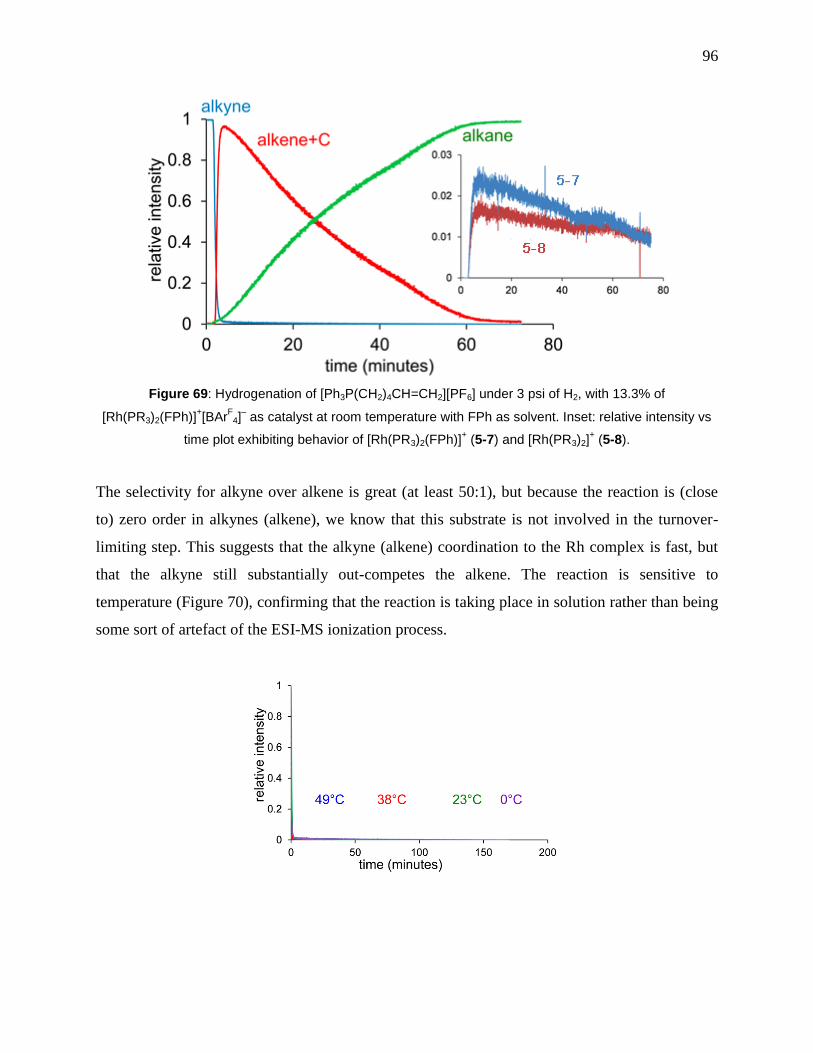
96
Figure 69: Hydrogenation of [Ph3P(CH2)4CH=CH2][PF6] under 3 psi of H2, with 13.3% of
[Rh(PR3)2(FPh)]+[BAr
F4]
– as catalyst at room temperature with FPh as solvent. Inset: relative intensity vs
time plot exhibiting behavior of [Rh(PR3)2(FPh)]+ (5-7) and [Rh(PR3)2]
+ (5-8).
The selectivity for alkyne over alkene is great (at least 50:1), but because the reaction is (close
to) zero order in alkynes (alkene), we know that this substrate is not involved in the turnover-
limiting step. This suggests that the alkyne (alkene) coordination to the Rh complex is fast, but
that the alkyne still substantially out-competes the alkene. The reaction is sensitive to
temperature (Figure 70), confirming that the reaction is taking place in solution rather than being
some sort of artefact of the ESI-MS ionization process.

97
Figure 70: Top: disappearance of alkyne 5-4 at 0, 23, 38 and 49°C (fast at all temperatures). Middle:
appearance and consumption of alkene 3. Bottom: appearance of alkane 5-6.
The reaction is first order in catalyst concentration (Figure 71), suggesting that the reaction
involves a mononuclear rhodium species as catalyst. Hydrogen was present in large excess
during the preliminary catalytic runs, so another experiment was carried out to establish the order
of this compound.
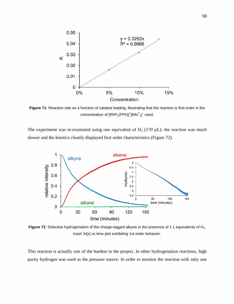
98
Figure 71: Reaction rate as a function of catalyst loading, illustrating that the reaction is first order in the
concentration of [RhP2(FPh)]+[BAr
F4]
– used.
The experiment was re-examined using one equivalent of H2 (170 µL): the reaction was much
slower and the kinetics cleanly displayed first order characteristics (Figure 72).
Figure 72: Selective hydrogenation of the charge-tagged alkyne in the presence of 1.1 equivalents of H2.
Inset: ln[x] vs time plot exhibiting 1st order behavior.
This reaction is actually one of the hardest in the project. In other hydrogenation reactions, high
purity hydrogen was used as the pressure source. In order to monitor the reaction with only one
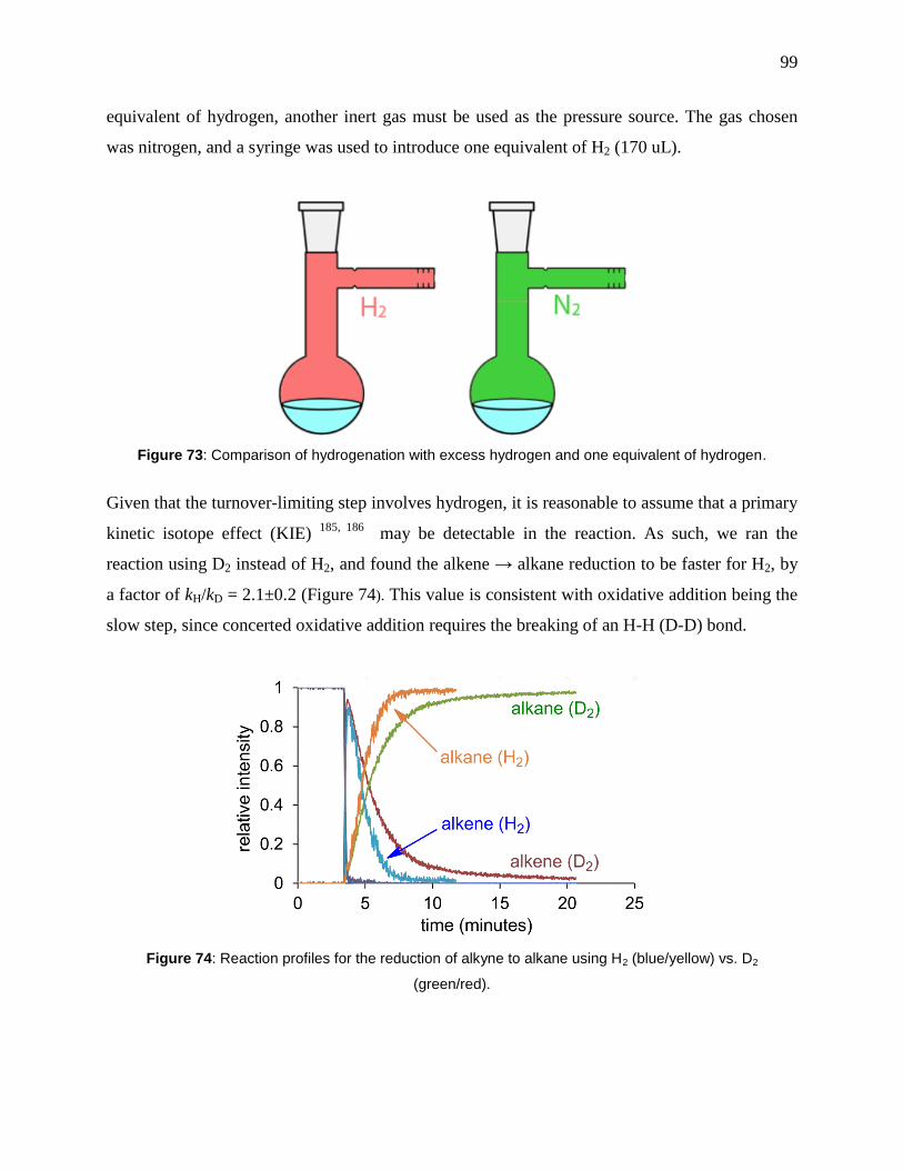
99
equivalent of hydrogen, another inert gas must be used as the pressure source. The gas chosen
was nitrogen, and a syringe was used to introduce one equivalent of H2 (170 uL).
Figure 73: Comparison of hydrogenation with excess hydrogen and one equivalent of hydrogen.
Given that the turnover-limiting step involves hydrogen, it is reasonable to assume that a primary
kinetic isotope effect (KIE) 185, 186
may be detectable in the reaction. As such, we ran the
reaction using D2 instead of H2, and found the alkene → alkane reduction to be faster for H2, by
a factor of kH/kD = 2.1±0.2 (Figure 74). This value is consistent with oxidative addition being the
slow step, since concerted oxidative addition requires the breaking of an H-H (D-D) bond.
Figure 74: Reaction profiles for the reduction of alkyne to alkane using H2 (blue/yellow) vs. D2
(green/red).
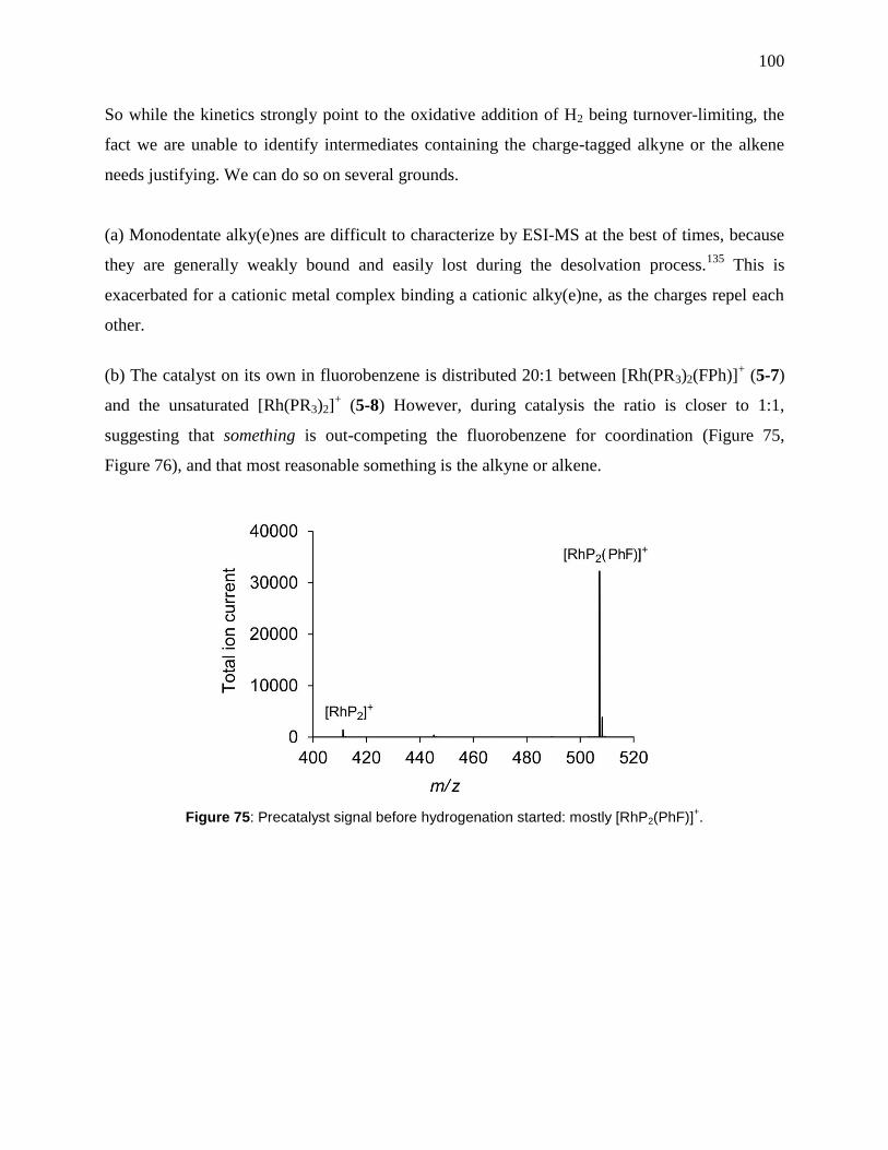
100
So while the kinetics strongly point to the oxidative addition of H2 being turnover-limiting, the
fact we are unable to identify intermediates containing the charge-tagged alkyne or the alkene
needs justifying. We can do so on several grounds.
(a) Monodentate alky(e)nes are difficult to characterize by ESI-MS at the best of times, because
they are generally weakly bound and easily lost during the desolvation process.135
This is
exacerbated for a cationic metal complex binding a cationic alky(e)ne, as the charges repel each
other.
(b) The catalyst on its own in fluorobenzene is distributed 20:1 between [Rh(PR3)2(FPh)]+ (5-7)
and the unsaturated [Rh(PR3)2]+ (5-8) However, during catalysis the ratio is closer to 1:1,
suggesting that something is out-competing the fluorobenzene for coordination (Figure 75,
Figure 76), and that most reasonable something is the alkyne or alkene.
Figure 75: Precatalyst signal before hydrogenation started: mostly [RhP2(PhF)]+.

101
Figure 76: Precatalyst signal after hydrogenation started: a mix of [RhP2]+ and [RhP2(PhF)]
+.
(c) Addition of octyne to [Rh(PR3)2(FPh)]+ displaces the fluorobenzene and produces the ions
[Rh(PR3)2(octyne)n]+ (n = 1 or 2, see Figure 77). This observation suggests that fluorobenzene is
a relatively weakly bound ligand and is easily displaced by alkynes. Interestingly, with different,
chelating ligands and CH2Cl2 as solvent, PhF dissociation is slow.187
Figure 77: Mass spectrum of [Rh(PR3)2(octyne)n]+ (n = 1, left, and n = 2, right). Experimental data shown
by line, calculated isotope pattern shown by columns.
(d) Mechanisms involving the alkyne (alkene) spending hardly any time coordinated to rhodium
(i.e. when the equilibria B ↔ C and B ↔ C’ lie a long way towards B) do not fit the observed
kinetics.
(e) Ions of the form [Rh(P2)H2]+ were never observed in the mass spectrometer in the presence of
H2, suggesting that addition of H2 to the catalyst is either slow or lies a long way in the wrong
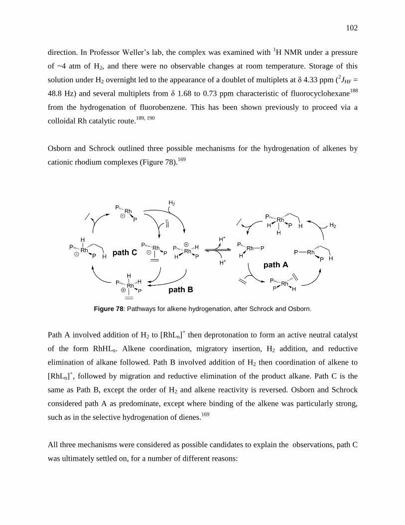
102
direction. In Professor Weller’s lab, the complex was examined with 1H NMR under a pressure
of ~4 atm of H2, and there were no observable changes at room temperature. Storage of this
solution under H2 overnight led to the appearance of a doublet of multiplets at δ 4.33 ppm (2JHF =
48.8 Hz) and several multiplets from δ 1.68 to 0.73 ppm characteristic of fluorocyclohexane188
from the hydrogenation of fluorobenzene. This has been shown previously to proceed via a
colloidal Rh catalytic route.189, 190
Osborn and Schrock outlined three possible mechanisms for the hydrogenation of alkenes by
cationic rhodium complexes (Figure 78).169
Figure 78: Pathways for alkene hydrogenation, after Schrock and Osborn.
Path A involved addition of H2 to [RhLn]+ then deprotonation to form an active neutral catalyst
of the form RhHLn. Alkene coordination, migratory insertion, H2 addition, and reductive
elimination of alkane followed. Path B involved addition of H2 then coordination of alkene to
[RhLn]+, followed by migration and reductive elimination of the product alkane. Path C is the
same as Path B, except the order of H2 and alkene reactivity is reversed. Osborn and Schrock
considered path A as predominate, except where binding of the alkene was particularly strong,
such as in the selective hydrogenation of dienes.169
All three mechanisms were considered as possible candidates to explain the observations, path C
was ultimately settled on, for a number of different reasons:

103
(a) Neither RhHLn (path A) nor [RhH2Ln]+ (path B) could be detected by
1H NMR when
examining [RhP2(fluorobenzene)]+ in the presence of H2.
(b) If Path A was operative, any of the intermediates RhHP2(alkene), RhRP2 and RhH2RP2 would
be observable as monocations using ESI-MS, thanks to the charged tag. None of these species
were in fact observed. If this path was operative, at least one should be (the one whose
consumption is turnover-limiting).
(c) Addition of bases such as NEt3 ought to accelerate reactions proceeding via Path A, thanks to
the deprotonation equilibrium being perturbed in the direction of RhHP2. However, no such
acceleration was observed. Indeed, the reaction was considerably slowed in the presence of NEt3
(Figure 79), and the reaction became much less selective for the alkyne. The reaction reached a
maximum of 50% in alkene only, similar to the degree of selectivity exhibited by Wilkinson’s
catalyst.95
Figure 79: The effect of NEt3 on the rate and selectivity of hydrogenation.
Note that addition of NEt3 to [RhP2]+ in the presence of H2 resulted in disappearance of [RhP2]
+
and the appearance of [HNEt3]+ (Figure 80), suggesting the formation of neutral RhHP2.
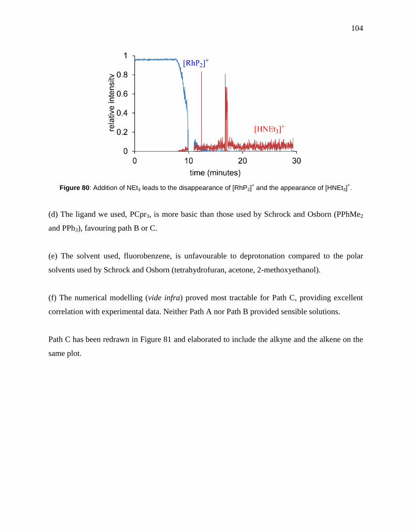
104
Figure 80: Addition of NEt3 leads to the disappearance of [RhP2]+ and the appearance of [HNEt3]
+.
(d) The ligand we used, PCpr3, is more basic than those used by Schrock and Osborn (PPhMe2
and PPh3), favouring path B or C.
(e) The solvent used, fluorobenzene, is unfavourable to deprotonation compared to the polar
solvents used by Schrock and Osborn (tetrahydrofuran, acetone, 2-methoxyethanol).
(f) The numerical modelling (vide infra) proved most tractable for Path C, providing excellent
correlation with experimental data. Neither Path A nor Path B provided sensible solutions.
Path C has been redrawn in Figure 81 and elaborated to include the alkyne and the alkene on the
same plot.
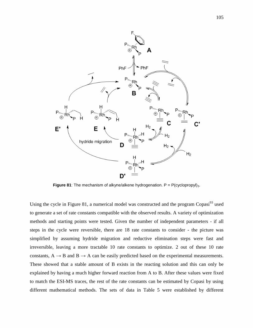
105
Figure 81: The mechanism of alkyne/alkene hydrogenation. P = P(cyclopropyl)3.
Using the cycle in Figure 81, a numerical model was constructed and the program Copasi93
used
to generate a set of rate constants compatible with the observed results. A variety of optimization
methods and starting points were tested. Given the number of independent parameters - if all
steps in the cycle were reversible, there are 18 rate constants to consider - the picture was
simplified by assuming hydride migration and reductive elimination steps were fast and
irreversible, leaving a more tractable 10 rate constants to optimize. 2 out of these 10 rate
constants, A → B and B → A can be easily predicted based on the experimental measurements.
These showed that a stable amount of B exists in the reacting solution and this can only be
explained by having a much higher forward reaction from A to B. After these values were fixed
to match the ESI-MS traces, the rest of the rate constants can be estimated by Copasi by using
different mathematical methods. The sets of data in Table 5 were established by different

106
methods: two different genetic algorithms, simulated annealing, differential evolution, and
evolutionary programming. For the computational methods, different starting points were
randomly chosen in order to ensure a local minimum hadn’t been found. All these methods
mentioned above generated very similar rate constants and they all provided a good match for
the experimental data.
Table 5: Estimated rate constants by different COPASI methods. First order rate constants are in units of
min-1
and second order rate constants in units of min-1
mmol-1
L.
Genetic
Algorithm
Genetic
Algorithm
SR
Simulated
Annealing
Differential
Evolution
Evolutionary
Programming
B → C 122 118 118 101 116
C → B 0.00364 0.122 1.175 × 10⁻⁵
0 4.37 × 10⁻⁶
B → C’ 4.79 4.43 4.67 3.39 4.56
C’ → B 0.0475 0.0412 0.0427 0 0.0404
C’ → D’ 1.92 2.01 1.95 2.06 2.13
D’ → C’ 2.00 329 2.72 0 925
C → D 0.0407 0.0408 0.0435 0.0410 0.0441
D → C 206 103 877 0 997
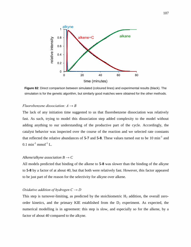
107
Figure 82: Direct comparison between simulated (coloured lines) and experimental results (black). The
simulation is for the genetic algorithm, but similarly good matches were obtained for the other methods.
Fluorobenzene dissociation: A → B
The lack of any initiation time suggested to us that fluorobenzene dissociation was relatively
fast. As such, trying to model this dissociation step added complexity to the model without
adding anything to our understanding of the productive part of the cycle. Accordingly, the
catalyst behavior was inspected over the course of the reaction and we selected rate constants
that reflected the relative abundances of 5-7 and 5-8. These values turned out to be 10 min-1
and
0.1 min-1
mmol-1
L.
Alkene/alkyne association B → C
All models predicted that binding of the alkene to 5-8 was slower than the binding of the alkyne
to 5-8 by a factor of at about 40, but that both were relatively fast. However, this factor appeared
to be just part of the reason for the selectivity for alkyne over alkene.
Oxidative addition of hydrogen C → D
This step is turnover-limiting, as predicted by the stoichiometric H2 addition, the overall zero-
order kinetics, and the primary KIE established from the D2 experiment. As expected, the
numerical modelling is in agreement: this step is slow, and especially so for the alkene, by a
factor of about 40 compared to the alkyne.

108
Migration and reductive elimination D → E and E -> B
No attempt was made to model these steps, since they must be relatively fast from all the other
evidence (most notably the observation of intermediates).
Further confirmation of the mechanism came through competition experiments. The charge-
tagged alkyne [Ph3P(CH2)4CCH]+ and a similar charge-tagged alkene, [Ph3P(CH2)3CH=CH2]
+
were combined and an excess H2 reduction was conducted competitively. Neither alkene reacted
until practically all of the alkyne was consumed, at which point the observed rates of alkene
consumption were fairly similar (Figure 83).
Figure 83: Competition reaction: reduction of alkyne vs. alkene. Note that the alkenes remain essentially
untouched until the alkyne is completely consumed. Reduction of the two alkenes proceed at similar
pace, though the hydrogenation of [Ph3P(CH2)3CH=CH2]+ was slightly faster than that of
[Ph3P(CH2)4CH=CH2]+.
The rate of reaction of the two alkenes are 3.2 × 10⁻⁴
mol L-1
min-1
for [Ph3P(CH2)3CH=CH2]+
and 2.5 × 10⁻⁴
mol L-1
min-1
for [Ph3P(CH2)4CH=CH2]+. The fractionally faster rate for
[Ph3P(CH2)3CH=CH2]+ is perhaps due to a small electronic effect due to the greater proximity of
the charged tag.
Examination of catalyst behavior showed that the ratio of 5-7 to 5-8 stayed fairly constant and
fairly similar in intensity throughout the reaction (see supporting information). The absolute
109
intensity reached a maximum soon after catalyst addition, and the intensity drops as the reaction
proceeds, stabilizing at the completion of the reaction. This behavior was attributed to a
competitive catalyst decomposition pathway stemming from a reaction intermediate (if the
decomposition was from a catalyst precursor, the decomposition ought to continue after the
cessation of the reaction). No charged rhodium-containing species were identified that could
account for the disappearance of signal, suggesting that the decomposition product is neutral.
RhP2H is one such possibility; there was no colour change that might indicate the formation of
metallic rhodium.
5.2.3 Conclusion
Analysis of alkyne hydrogenation using a charge-tagged alkyne and a cationic rhodium catalyst
revealed the catalyst to be a highly efficient partial hydrogenator, with a rate of alkyne
hydrogenation in excess of 50 times faster than alkene hydrogenation. The mechanism was
shown by a combination of ESI-MS, NMR, isotope effects and numerical modelling methods to
have a turnover-limiting step of oxidative addition of hydrogen following alkyne binding. Using
a stoichiometric amount of hydrogen was shown to be an effective means of enabling selective
hydrogenation to the alkene.
5.3 Experimental
Fluorobenzene was freshly distilled from P2O5 before use. All other solvents were dispensed
from an MBraun solvent purification system (SPS) immediately before use. All reactions were
under nitrogen or argon atmosphere. Chemicals and solvents were purchased from Aldrich and
used without subsequent purification. All mass spectra were collected by using a Micromass Q-
TOF micro mass spectrometer in positive ion mode using pneumatically assisted electrospray
ionization: capillary voltage, 3000 V; extraction voltage, 0.5 V; source temperature, 90°C;
desolvation temperature, 180°C; cone gas flow, 100 L/h; desolvation gas flow, 100 L/h;
collision voltage, 2 V (for MS experiments); collision voltage, 2-80 V (for MS/MS experiments);
MCP voltage, 2700 V.

110
ESI-MS reaction monitoring using pressurized sample infusion. A Schlenk flask was used
for these experiments, as described in Charpter 3.89, 90
A solution of [5-4][PF6] (10-20 mg,
0.021-0.042 mmol) was monitored using the PSI-ESI-MS setup. The Schlenk flask was
pressurized to 3 psi using 99.999% purity hydrogen gas or D2 gas. Wilkinson’s catalyst,
Rh(PPh3)3Cl (1.0-4.0 mg, 0.0011-0.0043 mmol) or [Rh(PCpr3)2(FPh)]+[BAr
F4]
– (1.0-6.0 mg,
0.75-4.5 µmol, 1.0-20.0% catalyst loading) was dissolved in 1.0 mL of fluorobenzene and
injected into the PSI flask via a septum. The solution end of PEEK tubing was protected with a
cannula filter system to avoid the tube being blocked by any insoluble by-products. Data were
processed by normalizing the abundance of each species to the total ion count of all species
identified as containing the tag. No smoothing of the data was performed.
5-2.Br. (4-ethynylbenzyl)triphenylphosphonium bromide. Triphenylphosphine (5.1 g, 19.6
mmol) and 4-iodobenzyl bromide (2.6 g, 8.7 mmol) were added to 10.0 mL toluene in a Schlenk
flask and the mixture was stirred for 72 hours. The solid product was dried under high vacuum
for 48 hours (4.9 g, 8.7 mmol, 99%). A portion of the product (0.30 g, 0.54 mmol) was mixed
with diisopropylamine (0.55 g 5.4 mmol), PdCl2(PPh3)2 (0.0019 g, 0.027 mmol), CuI (0.0010 g,
0.0054 mmol) and Me3SiC2H (0.11 g, 1.1 mmol) in a 12:5 mixture of MeOH and toluene and
allowed to react for 2 hours. Silica flash column was applied for purification, and the desired
product was isolated and dried to a brown powder (0.13 g, 0.28 mmol, 5.0%). Crystals for X-ray
crystallographic analysis were grown by vapour diffusion of hexane into a chloroform solution.
ESI-MS(+) m/z 377.1, (–) m/z 78.9.
5-2.PF6. (4-ethynylbenzyl)triphenylphosphonium hexafluorophosphate(V). Sodium
hexafluorophosphate (0.10 g, 0.60 mmol) was dissolved in 2.0 mL of water, and a 1 mL
methanol/water solution of 5-4.Br (0.030 g 0.065 mmol) was added with stirring. The product
was filtered and washed with water and dried under high vacuum for a week. The final product
was a white powder (0.028 g, 0.054 mmol, 83%). 1H NMR (CDCl3): δ (ppm) 7.82 (m, 3H); 7.68
(m, 7H); 7.55 (m, 7H); 6.89 (m, 2H); 4.61, (d, 2H, 14.4Hz); 3.10 (s, 1H). 31P NMR (CDCl3): δ
(ppm) 23.38 (singlet); -143.61 (septet). ESI-MS(+) m/z 377.1, (–) m/z 145.0.

111
5-3.Br. N,N-dioctyl-N-(prop-2-yn-1-yl)octan-1-aminium bromide. Trioctylamine (15.9 g,
45.1 mmol) and diethyl ether (10.0 mL) were introduced into an aluminium foil-wrapped
Schlenk flask at room temperature. Propargyl bromide (5.0 mL of an 80.0% solution in toluene)
was added, and the mixture stirred for 72 hours. The solvent was evaporated and the light brown
liquid dried under vacuum for 10 h. The final product was a light brown solid (19.8 g, 41.8
mmol, 93.0%). ESI-MS(+) m/z 392.6, (–) m/z 78.9.
5-3.PF6. N,N-dioctyl-N-(prop-2-yn-1-yl)octan-1-aminium hexafluorophosphate(V). A
methanol solution (10.0 ml) of 2.Br (5.3 g, 11.2 mmol) and sodium hexafluorophosphate (2.8 g,
16.7 mmol) was prepared. The mixture was added dropwise into 500.0 mL of distilled water and
stirred for 1 h. The yellow oily product was washed twice with 100.0 mL of distilled water under
sonication and dried under vacuum. Final product was a yellowish white powder (5.2 g, 9.7
mmol, 86.0%). 1H NMR (CDCl3): δ (ppm) 4.08 (d, 2H, 2.45Hz); 3.26 (m, 6H); 2.78 (m, 1H);
1.66 (m, 6H); 1.27, (m, 33H); 0.88 (m, 6H). ESI-MS(+) m/z 392.6, (–) m/z 145.0.
5-4.I. Hex-5-yn-1-yltriphenylphosphonium iodide. Triphenylphosphine (5.0 g, 19.0 mmol)
was dissolved into 10.0 mL of toluene in a Schlenk flask at 75oC, and 6-iodo-1-hexyne (1.0 g,
4.8 mmol) added dropwise over 10 minutes. The mixture was stirred for 72 hours, before the
product was filtered off, washed with toluene and dried under high vacuum. Final product was a
white powder (2.2 g, 4.7 mmol, 98.0%). Crystals for X-ray crystallographic analysis were grown
by vapour diffusion of hexane into a chloroform solution. ESI-MS(+) m/z 343.1, (–) m/z 126.9.
5-4.PF6. Hex-5-yn-1-yltriphenylphosphonium hexafluorophosphate(V). Sodium
hexafluorophosphate (0.56 g, 2.1 mmol) was dissolved in 5.0 mL of water, and 5.0 mL of a
methanol/water mixed solution of [Ph3P(CH2)4C2H]+[I]
– (0.50 g 1.1 mmol) was added dropwise
with stirring. The product was filtered and washed with water and dried under high vacuum for a
week. Final product was a white powder (0.55 g, 1.1 mmol, 53%). 1H NMR (CDCl3): δ (ppm)
7.81 (m, 3H); 7.70 (m, 12H); 3.22 (m, 2H); 2.29 (m, 2H); 1.86, (t, 1H, 2.64Hz); 1.81 (m, 3H);
1.26 (s, 1H). ESI-MS(+) m/z 343.1, (–) m/z 145.0.
112
5-9.Br. Pent-4-en-1-yltriphenylphosphonium bromide. Triphenylphosphine (5.5 g, 20.1
mmol) was dissolved into 10.0 mL of toluene in a Schlenk flask at 75oC, and 5-bromo-1-pentene
(2.1 g, 13.4 mmol) added dropwise over 10 minutes. The mixture was stirred for 72 hours, before
the product was filtered off, washed with toluene and dried under high vacuum. Final product
was a white powder (0.50 g, 1.2 mmol, 9.1%). ESI-MS(+) m/z 331.1, ESI-MS(–) m/z 78.9.
5-9.PF6. Pent-4-en-1-yltriphenylphosphonium hexafluorophosphate(V). Sodium
hexafluorophosphate (0.50 g, 3.0 mmol) was dissolved in 5.0 mL of water, and 5.0 mL of water
solution of [Ph3P(CH2)3C2H3]+[I]
– (0.50 g, 1.2 mmol,) was added dropwise with stirring. The
product was filtered and washed with water and dried under high vacuum for a week. Final
product was a white powder (0.5 g, 1.1 mmol, 91.0%). 1H NMR (CDCl3): δ (ppm) 7.80 (m, 3H);
7.68 (m, 12H); 5.68 (m, 1H); 5.05 (m, 2H); 3.13 (m, 2H); 2.30 (m, 2H); 1.71 (m, 2H). ESI-
MS(+) m/z 331.1, ESI-MS(–) m/z 145.0.

113
6. The use of charged substrates to investigate Si-H activation by ESI MS
I performed all experimental work, produced all figures and co-wrote the paper with JS
McIndoe. AG Oliver performed the crystal structure determinations, publication under
preparation.
Catalytic organosilicon chemistry has rapidly developed in recent years, especially Si-H
activation reactions. Catalytic Si-H activation is the process of coordination of Si-H σ bonds with
transition metals, followed by formation of a new Si-element bond, including dehydrocoupling
of silanes to make Si-Si bonds, hydrosilation to make Si-C bonds, silane hydrolysis and
alcoholysis to make Si-O bonds and so on. These reactions can be used to make functionalized
silicon compounds that have potential industrial applications such as silicone oil, rubber and
resin. However, structural control over the synthesis of the desired molecules remains limited by
relatively basic understanding of the mechanisms. The success of catalytic carbon reactions
cannot be directly copied into silicon because there are obvious differences in their electronic
structures.191
This chapter involves the preliminary investigation of catalytic reactions involving
Si-H bonds using the methods and strategies developed earlier in the thesis.
6.1 Current research in the area of Si-H activation
6.1.1 Dehydrocoupling of silane
Dehydrogenative coupling of silanes is a reaction involving breaking of Si-H bonds and
formation of a Si-Si bond, accompanied by the elimination of hydrogen gas. The product usually
involves the formation of oligo or polysilanes.192
Dehydrocoupling of silanes is an important
reaction because the products polysilanes have unusual thermal, photochemical, optical and
electronic properties which arise from the delocalization of sigma (σ) bonds in the backbone of
the oligomer, and this leads to the absorption of specific UV wavelengths by the Si-Si chain.193
Dehydrocoupling of silanes was first reported by Harrod when he investigated the
polymerization of organosilanes catalyzed by group IV complexes.194, 195
The advantages of
dehydrocoupling of silanes include easy purification (the main by-product is H2), the ability to
add functional groups, and control over stereochemistry and chain length. Dehydrocoupling of
silanes remains an active area of research, and catalysts used include early196,197
and late198-202
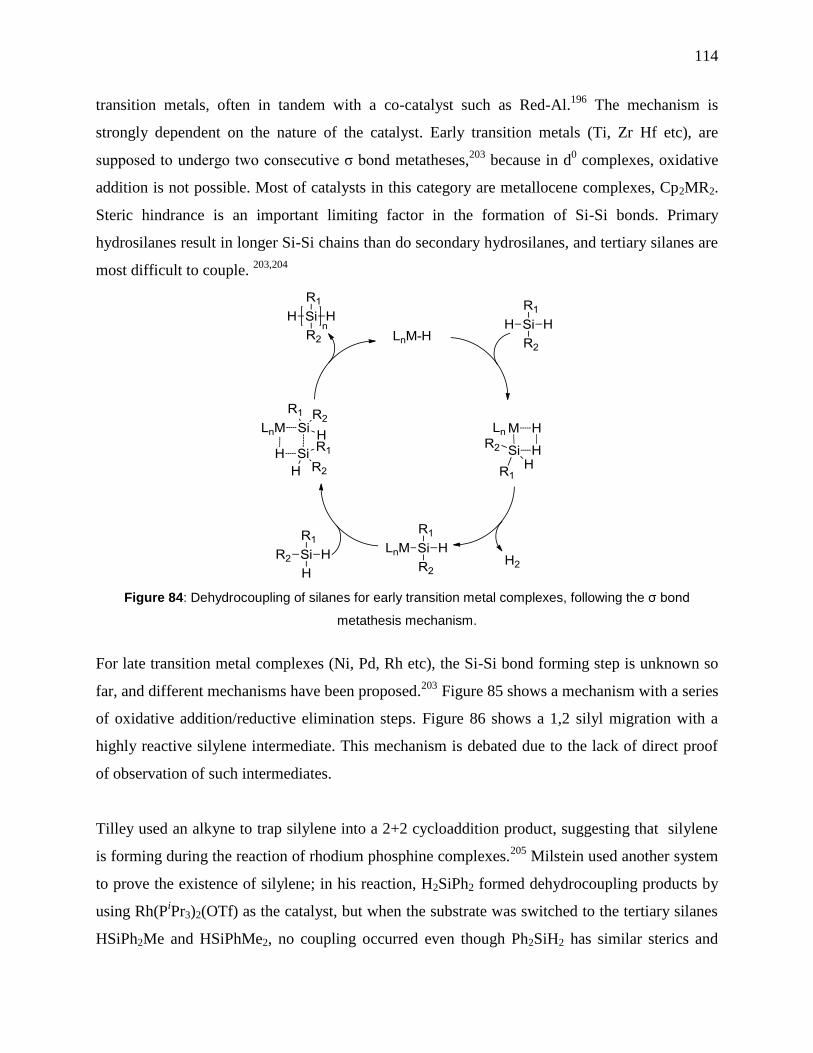
114
transition metals, often in tandem with a co-catalyst such as Red-Al.196
The mechanism is
strongly dependent on the nature of the catalyst. Early transition metals (Ti, Zr Hf etc), are
supposed to undergo two consecutive σ bond metatheses,203
because in d0 complexes, oxidative
addition is not possible. Most of catalysts in this category are metallocene complexes, Cp2MR2.
Steric hindrance is an important limiting factor in the formation of Si-Si bonds. Primary
hydrosilanes result in longer Si-Si chains than do secondary hydrosilanes, and tertiary silanes are
most difficult to couple. 203,204
Figure 84: Dehydrocoupling of silanes for early transition metal complexes, following the σ bond
metathesis mechanism.
For late transition metal complexes (Ni, Pd, Rh etc), the Si-Si bond forming step is unknown so
far, and different mechanisms have been proposed.203
Figure 85 shows a mechanism with a series
of oxidative addition/reductive elimination steps. Figure 86 shows a 1,2 silyl migration with a
highly reactive silylene intermediate. This mechanism is debated due to the lack of direct proof
of observation of such intermediates.
Tilley used an alkyne to trap silylene into a 2+2 cycloaddition product, suggesting that silylene
is forming during the reaction of rhodium phosphine complexes.205
Milstein used another system
to prove the existence of silylene; in his reaction, H2SiPh2 formed dehydrocoupling products by
using Rh(PiPr3)2(OTf) as the catalyst, but when the substrate was switched to the tertiary silanes
HSiPh2Me and HSiPhMe2, no coupling occurred even though Ph2SiH2 has similar sterics and
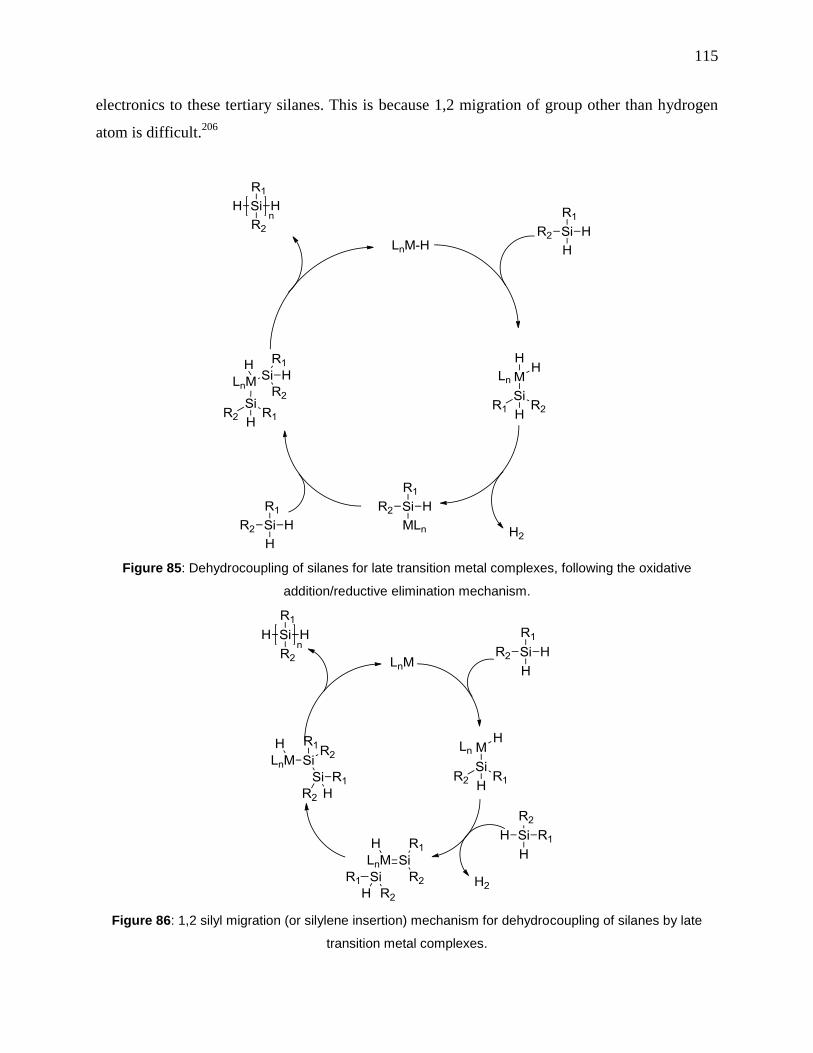
115
electronics to these tertiary silanes. This is because 1,2 migration of group other than hydrogen
atom is difficult.206
Figure 85: Dehydrocoupling of silanes for late transition metal complexes, following the oxidative
addition/reductive elimination mechanism.
Figure 86: 1,2 silyl migration (or silylene insertion) mechanism for dehydrocoupling of silanes by late
transition metal complexes.
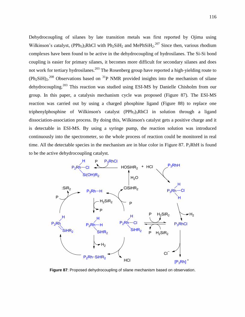
116
Dehydrocoupling of silanes by late transition metals was first reported by Ojima using
Wilkinson’s catalyst, (PPh3)3RhCl with Ph2SiH2 and MePhSiH2.207
Since then, various rhodium
complexes have been found to be active in the dehydrocoupling of hydrosilanes. The Si-Si bond
coupling is easier for primary silanes, it becomes more difficult for secondary silanes and does
not work for tertiary hydrosilanes.203
The Rosenberg group have reported a high-yielding route to
(Ph2SiH)2.208
Observations based on 31
P NMR provided insights into the mechanism of silane
dehydrocoupling.203
This reaction was studied using ESI-MS by Danielle Chisholm from our
group. In this paper, a catalysis mechanism cycle was proposed (Figure 87). The ESI-MS
reaction was carried out by using a charged phosphine ligand (Figure 88) to replace one
triphenylphosphine of Wilkinson's catalyst (PPh3)3RhCl in solution through a ligand
dissociation-association process. By doing this, Wilkinson's catalyst gets a positive charge and it
is detectable in ESI-MS. By using a syringe pump, the reaction solution was introduced
continuously into the spectrometer, so the whole process of reaction could be monitored in real
time. All the detectable species in the mechanism are in blue color in Figure 87. P2RhH is found
to be the active dehydrocoupling catalyst.
Figure 87: Proposed dehydrocoupling of silane mechanism based on observation.
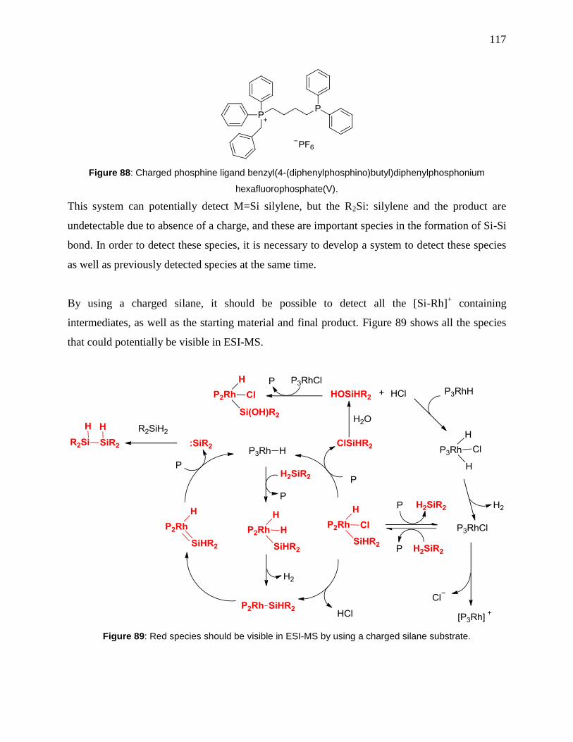
117
Figure 88: Charged phosphine ligand benzyl(4-(diphenylphosphino)butyl)diphenylphosphonium
hexafluorophosphate(V).
This system can potentially detect M=Si silylene, but the R2Si: silylene and the product are
undetectable due to absence of a charge, and these are important species in the formation of Si-Si
bond. In order to detect these species, it is necessary to develop a system to detect these species
as well as previously detected species at the same time.
By using a charged silane, it should be possible to detect all the [Si-Rh]+ containing
intermediates, as well as the starting material and final product. Figure 89 shows all the species
that could potentially be visible in ESI-MS.
Figure 89: Red species should be visible in ESI-MS by using a charged silane substrate.

118
6.1.2 Hydrolysis of silanes
Siloxanes and polysiloxanes are valuable building blocks for silicon-based polymeric materials
in industry.209
Global demand for siloxanes and polysiloxanes was about 13.5 billion dollars in
2010210
. Usually the synthesis involves the strongly exothermic hydrolysis of chlorosilanes by
water to generate silanediols, which condense into polysiloxanes.211
Corrosive HCl gas is
released during the reaction (Figure 90).
Figure 90: Hydrolysis of diclorosilane
Another method to make these materials is by hydrolysis of hydrosilanes with water. This
method will not generate HCl and the only by-product is hydrogen gas, so it is environmentally
friendly and has high atom economy. However, even though there is huge bond energy
difference between Si-H and Si-O bond, the conversion of Si-H into Si-O bond by water is quite
slow in neutral conditions. Base and strong acid are commonly used as catalysts,211
however
metal catalysts become more popular because their highly efficient behaviour and mild reaction
conditions.
Hydrolysis of silane with water by organometallic catalysts has become a hot topic in the last
decade.209, 212-220
By using different equivalents of water and various types of catalysts,
hydrosilanes will react with water to generate siloxanes, polysiloxanes and hydrogen gas, and
condensation reaction between siloxanes will generate polysiloxanes and water (Figure 91).221
Figure 91: Hydrolysis and condensation of hydrosilanes.
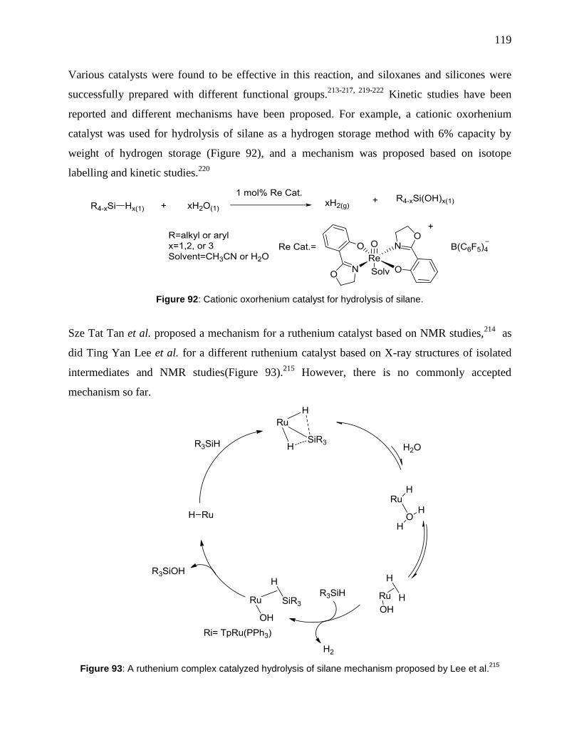
119
Various catalysts were found to be effective in this reaction, and siloxanes and silicones were
successfully prepared with different functional groups.213-217, 219-222
Kinetic studies have been
reported and different mechanisms have been proposed. For example, a cationic oxorhenium
catalyst was used for hydrolysis of silane as a hydrogen storage method with 6% capacity by
weight of hydrogen storage (Figure 92), and a mechanism was proposed based on isotope
labelling and kinetic studies.220
Figure 92: Cationic oxorhenium catalyst for hydrolysis of silane.
Sze Tat Tan et al. proposed a mechanism for a ruthenium catalyst based on NMR studies,214
as
did Ting Yan Lee et al. for a different ruthenium catalyst based on X-ray structures of isolated
intermediates and NMR studies(Figure 93).215
However, there is no commonly accepted
mechanism so far.
Figure 93: A ruthenium complex catalyzed hydrolysis of silane mechanism proposed by Lee et al.215

120
6.1.3 Hydrosilation
Hydrosilation is one of the most important techniques for making an Si-C bond as well as other
silicon-heteroelement bonds by addition of Si-H to a π bond (C=C, C≡C etc).211, 223
It can
introduce functionalized silanes or alkylsilanes into organic molecules (Si-Cl, Si-OR etc.).
Hydrosilation can be mediated by radicals and transition metal catalysts.4 In this thesis, transition
metal catalyzed hydrosilation will be focused on.
Bart reported a new Fe(0) complex (Figure 94) that is efficient and regiospecific for
hydrosilation of terminal alkenes with PhSiH3 and Ph2SiH2. After hydrosilation, styrene will only
go to the terminal hydrosilation product (Scheme 12). This research showed how new ligands
can be helpful for modulating metal activity, and how non-precious metals can effectively
catalyze hydrosilation.224
Scheme 12: Exclusive terminal hydrosilation product.
Figure 94: Fe complex for hydrosilation
Platinum catalysts, such Karstedt's catalyst, are very efficient in hydrosilation reactions.225-228
[Cp*Ru(MeCN)3][PF6] is very efficient for the hydrosilation of alkynes, with mainly α-addition
products.229-233
Many other transition metals can also be used in hydrosilation, including Pt,234
Fe,224
Ru,235, 236
Os,237
Rh,238, 239
Ir,240, 241
and Ni.242
However, for such a widely used reaction,
there are still problems with hydrosilation catalyst design, especially in terms of stereoselectivity,
partly because it is hard to isolate and characterize the extremely reactive intermediates. The
commonly accepted mechanism for the hydrosilation was proposed by Chalk and Harrod, who
made an analogy between isolated Ir complexes and their proposed reactive Pt catalyst species
(Figure 95). 223
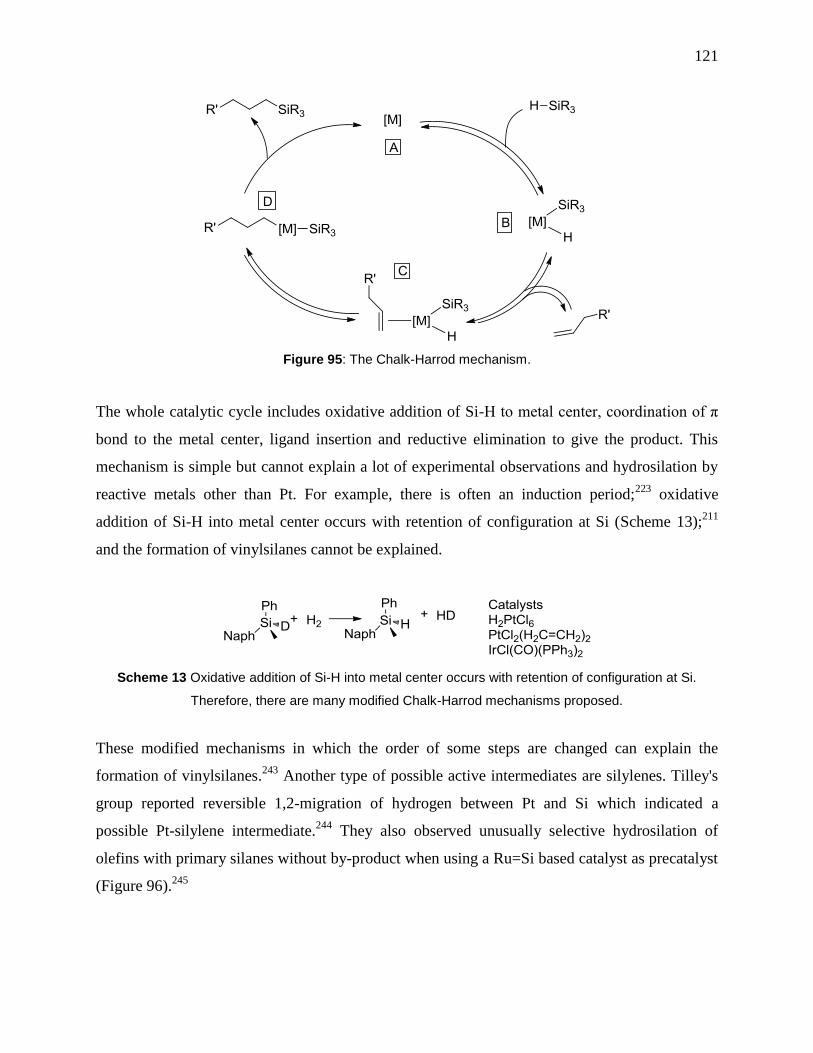
121
Figure 95: The Chalk-Harrod mechanism.
The whole catalytic cycle includes oxidative addition of Si-H to metal center, coordination of π
bond to the metal center, ligand insertion and reductive elimination to give the product. This
mechanism is simple but cannot explain a lot of experimental observations and hydrosilation by
reactive metals other than Pt. For example, there is often an induction period;223
oxidative
addition of Si-H into metal center occurs with retention of configuration at Si (Scheme 13);211
and the formation of vinylsilanes cannot be explained.
Scheme 13 Oxidative addition of Si-H into metal center occurs with retention of configuration at Si.
Therefore, there are many modified Chalk-Harrod mechanisms proposed.
These modified mechanisms in which the order of some steps are changed can explain the
formation of vinylsilanes.243
Another type of possible active intermediates are silylenes. Tilley's
group reported reversible 1,2-migration of hydrogen between Pt and Si which indicated a
possible Pt-silylene intermediate.244
They also observed unusually selective hydrosilation of
olefins with primary silanes without by-product when using a Ru=Si based catalyst as precatalyst
(Figure 96).245

122
Figure 96: Proposed Ru–silylene-based catalytic cycle.
These are just a very small part of the whole mechanism investigation of hydrosilation research,
and many new research results were published recently. However there are still many problems
unexplainable so far, the understanding of catalytic cycle based on currently scientific
methodology has been very slow and design of a good asymmetric catalyst is still largely
dependent on “a mixture of luck, intuition and perseverance”.246
It is necessary to get new
techniques involved in the area.
6.2 Results and Discussion
For synthesizing charged hydrosilanes, different synthetic routes were attempted. (Scheme 14)
Compound 6-4 and 6-5 are stable and easy to prepare, and Figure 97 shows the X-ray crystal
structure of 6-5.

123
Scheme 14: Attempted routes for making charged silane substrates.
Figure 97: X-ray crystal structure of compound 6-5.
With the synthesized charged substrate 6-5, PSI-ESI-MS89
was used as sampling method.
Comparing with syringe pump sampling method, PSI-ESI-MS gives much better results, and it
can monitor the whole reaction from the very beginning. Figure 98 shows the reaction
investigated. By adding 10 equivalents of di-n-hexylsilane, the chance of double charged species
is decreased, the Si-Si chain can grow longer, and the concentration of the charged species is
kept reasonably low.
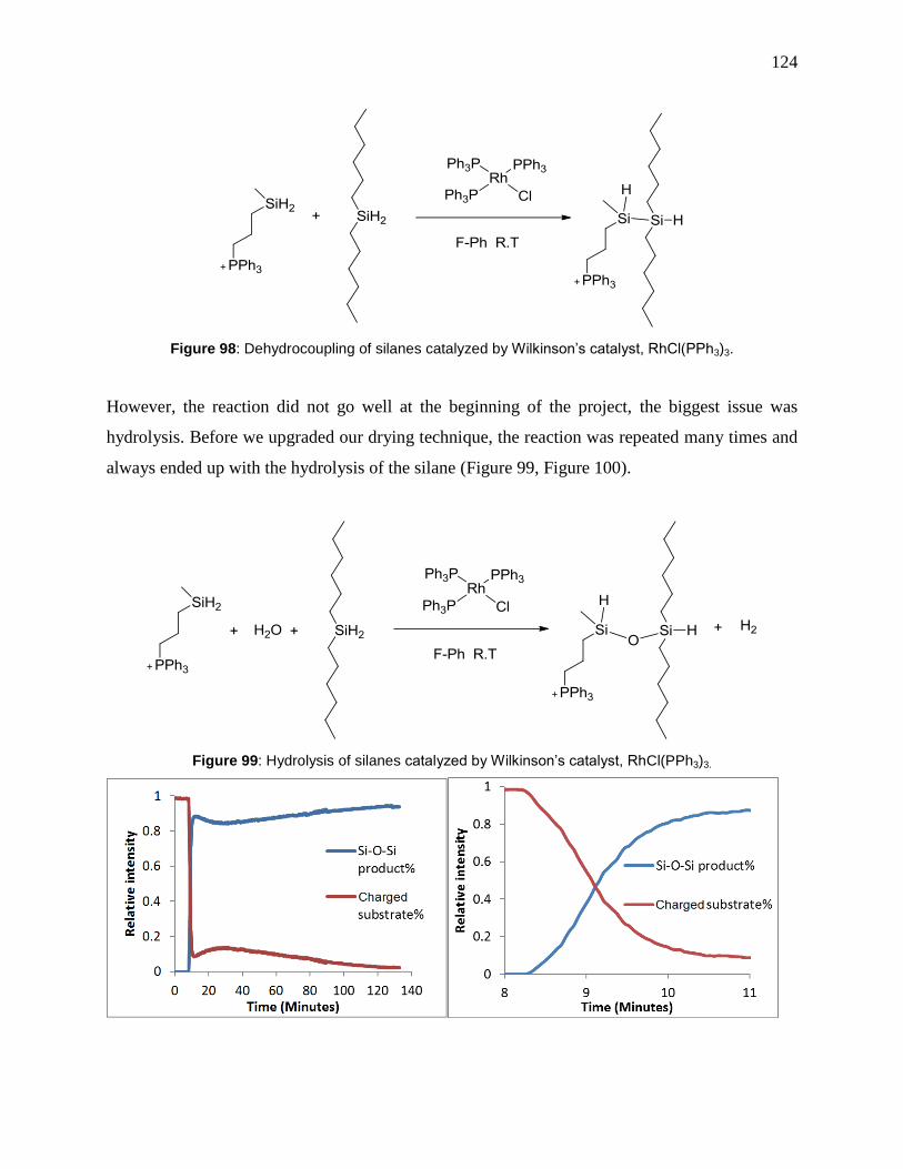
124
Figure 98: Dehydrocoupling of silanes catalyzed by Wilkinson’s catalyst, RhCl(PPh3)3.
However, the reaction did not go well at the beginning of the project, the biggest issue was
hydrolysis. Before we upgraded our drying technique, the reaction was repeated many times and
always ended up with the hydrolysis of the silane (Figure 99, Figure 100).
Figure 99: Hydrolysis of silanes catalyzed by Wilkinson’s catalyst, RhCl(PPh3)3.
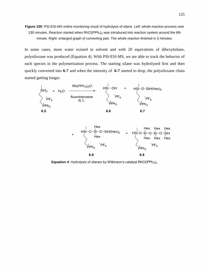
125
Figure 100: PSI-ESI-MS online monitoring result of hydrolysis of silane. Left: whole reaction process over
130 minutes. Reaction started when RhCl(PPh3)3 was introduced into reaction system around the 8th
minute. Right: enlarged graph of converting part. The whole reaction finished in 3 minutes.
In some cases, more water existed in solvent and with 20 equivalents of dihexylsilane,
polysiloxane was produced (Equation 4). With PSI-ESI-MS, we are able to track the behavior of
each species in the polymerization process. The starting silane was hydrolyzed first and then
quickly converted into 6-7 and when the intensity of 6-7 started to drop, the polysiloxane chain
started getting longer.
Equation 4: Hydrolysis of silanes by Wilkinson’s catalyst RhCl(PPh3)3.

126
Figure 101: PSI-ESI-MS online monitoring result of hydrolysis of silane. Whole reaction process was over
210 minutes. Reaction started when RhCl(PPh3)3 was introduced into reaction system around the 10th
minute.
During the investigation of alkyne hydrosilation, a similar hydrolysis reaction was recorded
(Figure 102, Figure 103). The oligomerization reaction kept going on as long as water was
present.
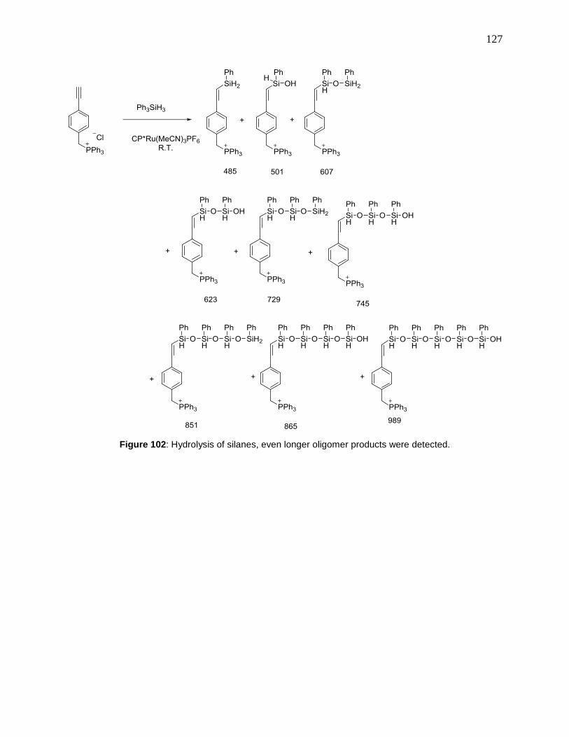
127
Figure 102: Hydrolysis of silanes, even longer oligomer products were detected.
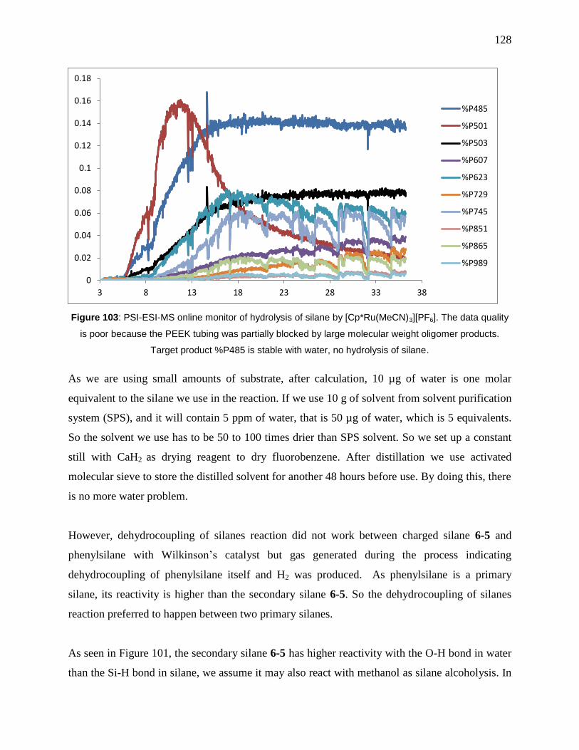
128
Figure 103: PSI-ESI-MS online monitor of hydrolysis of silane by [Cp*Ru(MeCN)3][PF6]. The data quality
is poor because the PEEK tubing was partially blocked by large molecular weight oligomer products.
Target product %P485 is stable with water, no hydrolysis of silane.
As we are using small amounts of substrate, after calculation, 10 µg of water is one molar
equivalent to the silane we use in the reaction. If we use 10 g of solvent from solvent purification
system (SPS), and it will contain 5 ppm of water, that is 50 µg of water, which is 5 equivalents.
So the solvent we use has to be 50 to 100 times drier than SPS solvent. So we set up a constant
still with CaH2 as drying reagent to dry fluorobenzene. After distillation we use activated
molecular sieve to store the distilled solvent for another 48 hours before use. By doing this, there
is no more water problem.
However, dehydrocoupling of silanes reaction did not work between charged silane 6-5 and
phenylsilane with Wilkinson’s catalyst but gas generated during the process indicating
dehydrocoupling of phenylsilane itself and H2 was produced. As phenylsilane is a primary
silane, its reactivity is higher than the secondary silane 6-5. So the dehydrocoupling of silanes
reaction preferred to happen between two primary silanes.
As seen in Figure 101, the secondary silane 6-5 has higher reactivity with the O-H bond in water
than the Si-H bond in silane, we assume it may also react with methanol as silane alcoholysis. In
0
0.02
0.04
0.06
0.08
0.1
0.12
0.14
0.16
0.18
3 8 13 18 23 28 33 38
%P485
%P501
%P503
%P607
%P623
%P729
%P745
%P851
%P865
%P989
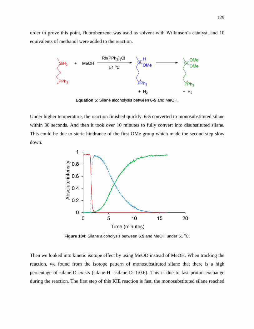
129
order to prove this point, fluorobenzene was used as solvent with Wilkinson’s catalyst, and 10
equivalents of methanol were added to the reaction.
Equation 5: Silane alcoholysis between 6-5 and MeOH.
Under higher temperature, the reaction finished quickly. 6-5 converted to monosubstituted silane
within 30 seconds. And then it took over 10 minutes to fully convert into disubstituted silane.
This could be due to steric hindrance of the first OMe group which made the second step slow
down.
Figure 104: Silane alcoholysis between 6.5 and MeOH under 51 oC.
Then we looked into kinetic isotope effect by using MeOD instead of MeOH. When tracking the
reaction, we found from the isotope pattern of monosubstituted silane that there is a high
percentage of silane-D exists (silane-H : silane-D=1:0.6). This is due to fast proton exchange
during the reaction. The first step of this KIE reaction is fast, the monosubstituted silane reached
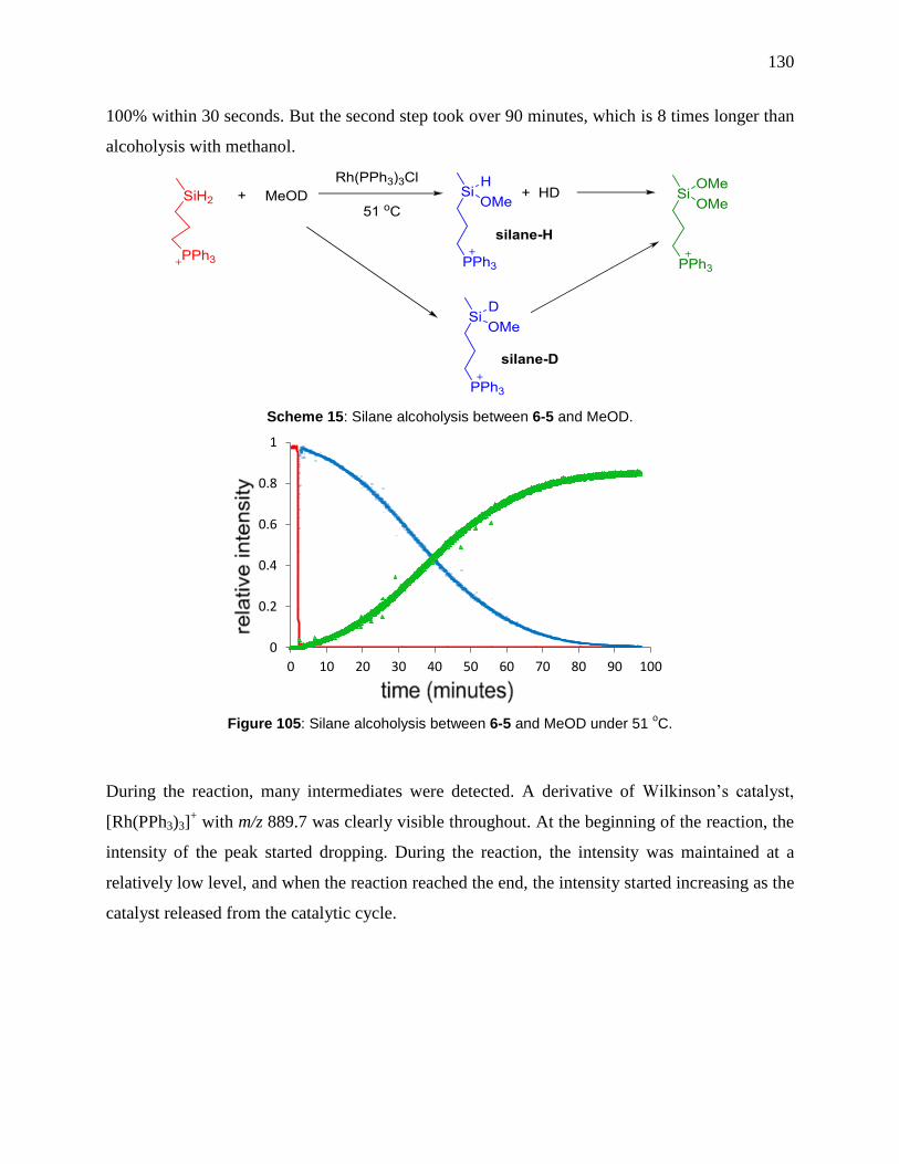
130
100% within 30 seconds. But the second step took over 90 minutes, which is 8 times longer than
alcoholysis with methanol.
Scheme 15: Silane alcoholysis between 6-5 and MeOD.
Figure 105: Silane alcoholysis between 6-5 and MeOD under 51 oC.
During the reaction, many intermediates were detected. A derivative of Wilkinson’s catalyst,
[Rh(PPh3)3]+ with m/z 889.7 was clearly visible throughout. At the beginning of the reaction, the
intensity of the peak started dropping. During the reaction, the intensity was maintained at a
relatively low level, and when the reaction reached the end, the intensity started increasing as the
catalyst released from the catalytic cycle.
0
0.2
0.4
0.6
0.8
1
0 10 20 30 40 50 60 70 80 90 100
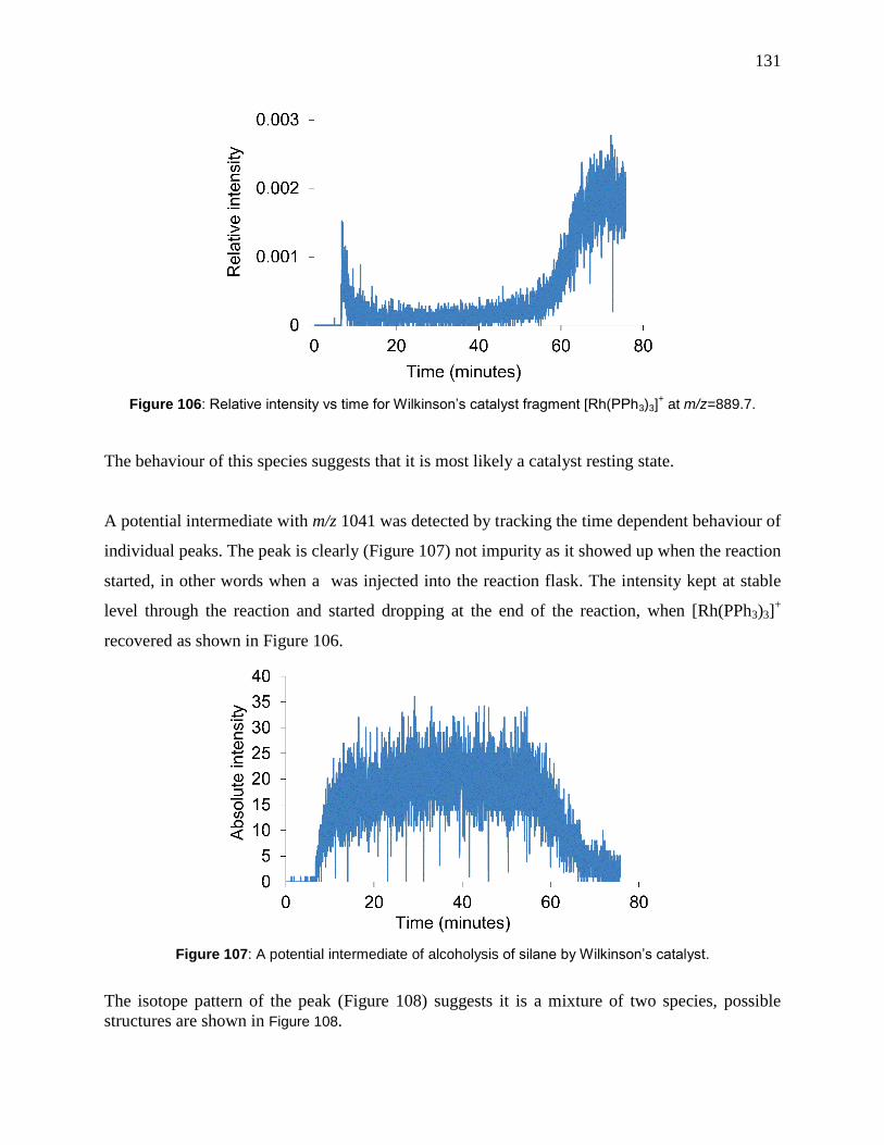
131
Figure 106: Relative intensity vs time for Wilkinson’s catalyst fragment [Rh(PPh3)3]+ at m/z=889.7.
The behaviour of this species suggests that it is most likely a catalyst resting state.
A potential intermediate with m/z 1041 was detected by tracking the time dependent behaviour of
individual peaks. The peak is clearly (Figure 107) not impurity as it showed up when the reaction
started, in other words when a was injected into the reaction flask. The intensity kept at stable
level through the reaction and started dropping at the end of the reaction, when [Rh(PPh3)3]+
recovered as shown in Figure 106.
Figure 107: A potential intermediate of alcoholysis of silane by Wilkinson’s catalyst.
The isotope pattern of the peak (Figure 108) suggests it is a mixture of two species, possible
structures are shown in Figure 108.
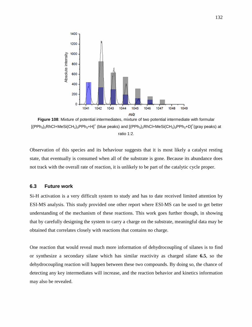
132
Figure 108: Mixture of potential intermediates, mixture of two potential intermediate with formular
[(PPh3)2RhCl+MeSi(CH2)3PPh3+H]+ (blue peaks) and [(PPh3)2RhCl+MeSi(CH2)3PPh3+D]
+(gray peaks) at
ratio 1:2.
Observation of this species and its behaviour suggests that it is most likely a catalyst resting
state, that eventually is consumed when all of the substrate is gone. Because its abundance does
not track with the overall rate of reaction, it is unlikely to be part of the catalytic cycle proper.
6.3 Future work
Si-H activation is a very difficult system to study and has to date received limited attention by
ESI-MS analysis. This study provided one other report where ESI-MS can be used to get better
understanding of the mechanism of these reactions. This work goes further though, in showing
that by carefully designing the system to carry a charge on the substrate, meaningful data may be
obtained that correlates closely with reactions that contains no charge.
One reaction that would reveal much more information of dehydrocoupling of silanes is to find
or synthesize a secondary silane which has similar reactivity as charged silane 6.5, so the
dehydrocoupling reaction will happen between these two compounds. By doing so, the chance of
detecting any key intermediates will increase, and the reaction behavior and kinetics information
may also be revealed.

133
The silane alcoholysis reaction also has great potential for studying the mechanism,
characterizing different intermediates and build numerical models. Different temperature and
different alcohols can be used to see the influence of functional groups. CD3OD and other
deuterated alcohol can be used for study of the kinetic isotope effect.
6.4 Experimental
Fluorobenzene was freshly distilled from CaH2 and stored over molecualr sievesbefore use. All
other solvents were dispensed from an MBraun solvent purification system (SPS) immediately
before use. All reactions were under nitrogen or argon atmosphere. Chemicals and solvents were
purchased from Aldrich and used without subsequent purification. All mass spectra were
collected by using a Micromass Q-TOF micro mass spectrometer in positive ion mode using
pneumatically assisted electrospray ionization: capillary voltage, 3000 V; extraction voltage, 0.5
V; source temperature, 90°C; desolvation temperature, 180°C; cone gas flow, 100 L/h;
desolvation gas flow, 100 L/h; collision voltage, 2 V (for MS experiments); collision voltage, 2-
80 V (for MS/MS experiments); MCP voltage, 2700 V.
ESI-MS reaction monitoring using pressurized sample infusion. A Schlenk flask was used
for these experiments, as described elsewhere.89, 90
A solution of [6.5][PF6] (5-10 mg, 0.010-
0.020 mmol) was monitored using the PSI-ESI-MS setup. The Schlenk flask was pressurized to 3
psi using 99.999% purity N2 gas or Ar gas. Wilkinson’s catalyst, Rh(PPh3)3Cl (1-4 mg, 0.0011-
0.0043 mmol) was dissolved in 1 mL of fluorobenzene and injected into the PSI flask via a
septum. The solution end of PEEK tubing was protected with a cannula filter system to avoid the
tube being blocked by any insoluble by-products. Data were processed by normalizing the
abundance of each species to the total ion count of all species identified as containing the tag. No
smoothing of the data was performed.
Dihexylsilane. LiAlH4 (6.2 g, 163.0 mmol) and 200.0 ml of tetraglyme were introduced into a
three neck round bottom flask. Di-n-hexyldichlorosilane (25.0 ml, 81.5 mmol) was introduced
into the same flask dropwise over 30 minutes in ice bath. The reaction was stirred at room
temperature overnight. The mixture was vacuum distilled and the product fraction collected at
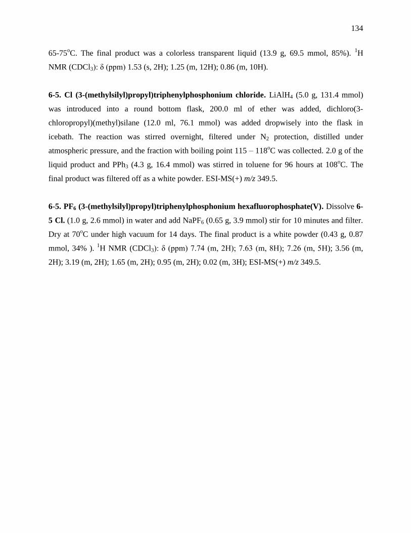
134
65-75oC. The final product was a colorless transparent liquid (13.9 g, 69.5 mmol, 85%).
1H
NMR (CDCl3): δ (ppm) 1.53 (s, 2H); 1.25 (m, 12H); 0.86 (m, 10H).
6-5. Cl (3-(methylsilyl)propyl)triphenylphosphonium chloride. LiAlH4 (5.0 g, 131.4 mmol)
was introduced into a round bottom flask, 200.0 ml of ether was added, dichloro(3-
chloropropyl)(methyl)silane (12.0 ml, 76.1 mmol) was added dropwisely into the flask in
icebath. The reaction was stirred overnight, filtered under N2 protection, distilled under
atmospheric pressure, and the fraction with boiling point 115 – 118oC was collected. 2.0 g of the
liquid product and PPh3 (4.3 g, 16.4 mmol) was stirred in toluene for 96 hours at 108oC. The
final product was filtered off as a white powder. ESI-MS(+) m/z 349.5.
6-5. PF6 (3-(methylsilyl)propyl)triphenylphosphonium hexafluorophosphate(V). Dissolve 6-
5 Cl. (1.0 g, 2.6 mmol) in water and add NaPF6 (0.65 g, 3.9 mmol) stir for 10 minutes and filter.
Dry at 70oC under high vacuum for 14 days. The final product is a white powder (0.43 g, 0.87
mmol, 34% ). 1H NMR (CDCl3): δ (ppm) 7.74 (m, 2H); 7.63 (m, 8H); 7.26 (m, 5H); 3.56 (m,
2H); 3.19 (m, 2H); 1.65 (m, 2H); 0.95 (m, 2H); 0.02 (m, 3H); ESI-MS(+) m/z 349.5.

135
7. Collaborative studies
Portions of this chapter have been previously published, and are reproduced in part with
permission from “Copper-Mediated Fluorination of Arylboronate Esters. Identification of a
Copper(III) Fluoride Complex” P. S. Fier, J. Luo and J. F. Hartwig, Journal of the American
Chemical Society, 2013, 135, 2552-2559. Copyright © 2013 American Chemical Society
I performed all experimental work, produced all figures and co-wrote the paper with JS McIndoe
and collaborators. Publications are under preparation.
As the importance of organometallic compounds increase every day, more and more air and
moisture sensitive catalysts and molecules are synthesised. Scientists are seeking new ways to
understand the behaviour and reactivity of their systems, and ESI-MS can often provide new and
complementary information. Follow-up analyses may include MS/MS experiments that can
provide further characterization of species of interest. However, many groups lack the
infrastructure and expertise to conduct the necessary experiments, and seek to collaborate with us
to provide unique insights. This chapter provides brief accounts of some of these collaborations;
so far one paper has been published247
and more are on the way.
7.1 CdSe-DHLA for H2 production
Professor Patrick Holland and Professor Richard Eisenberg from the University of Rochester
have been working on hydrogen production system by using water as solvent at pH 4.5, ascorbic
acid (AA) (0.5-1 M) as the sacrificial donor, CdSe quantum dot (4.0 µM) capped with
dihydrolipoic acid (DHLA ~400 µM) as the photosensitizer, and Ni(NO3)2 (4.0 µM) as the pre-
catalyst. Lots of work had been done to prove that the Ni was not attached to the CdSe. The
hypothesis was that the Ni2+
forms a complex with DHLA, which has been shown to be able to
detach from CdSe under photolysis, but it was not known how much DHLA came off the CdSe
surface and how it coordinated to the Ni2+
.
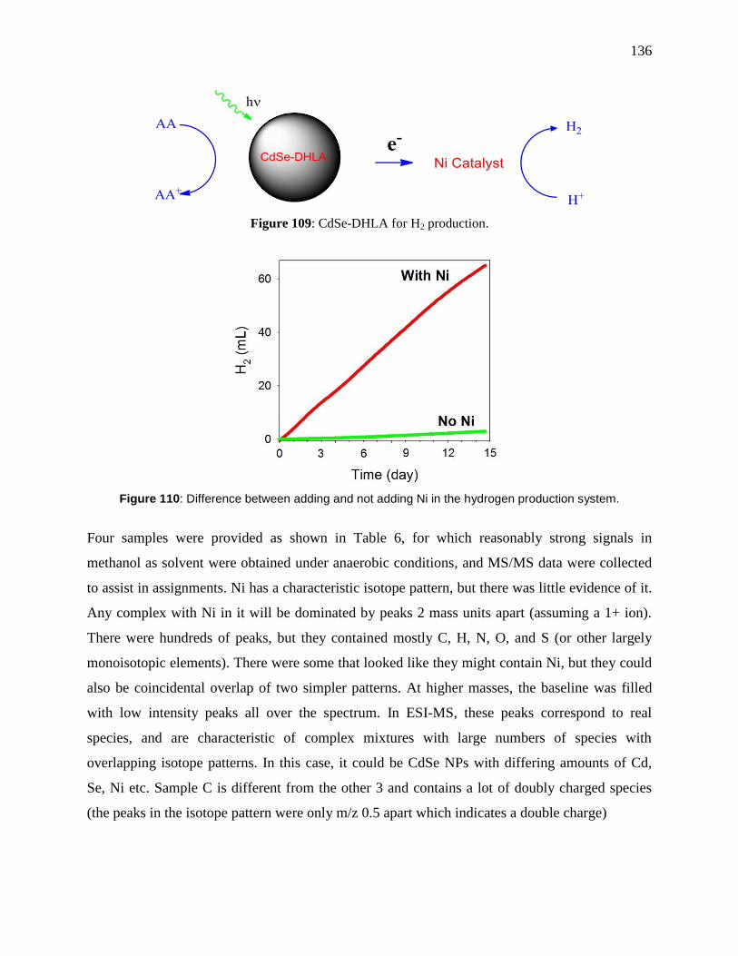
136
Figure 109: CdSe-DHLA for H2 production.
Figure 110: Difference between adding and not adding Ni in the hydrogen production system.
Four samples were provided as shown in Table 6, for which reasonably strong signals in
methanol as solvent were obtained under anaerobic conditions, and MS/MS data were collected
to assist in assignments. Ni has a characteristic isotope pattern, but there was little evidence of it.
Any complex with Ni in it will be dominated by peaks 2 mass units apart (assuming a 1+ ion).
There were hundreds of peaks, but they contained mostly C, H, N, O, and S (or other largely
monoisotopic elements). There were some that looked like they might contain Ni, but they could
also be coincidental overlap of two simpler patterns. At higher masses, the baseline was filled
with low intensity peaks all over the spectrum. In ESI-MS, these peaks correspond to real
species, and are characteristic of complex mixtures with large numbers of species with
overlapping isotope patterns. In this case, it could be CdSe NPs with differing amounts of Cd,
Se, Ni etc. Sample C is different from the other 3 and contains a lot of doubly charged species
(the peaks in the isotope pattern were only m/z 0.5 apart which indicates a double charge)

137
Table 6: Samples for CdSe-DHLA for H2 production
Ascorbic Acid CdSe-DHLA Ni(NO3)2 pH Reaction Time
(hv > 450 nm)
Sample A 16 µM 4 µM 4 µM 4.5 1 hour
Sample B 16 µM 4 µM 4 µM 4.5 5 hour
Sample C 0.3 M 4 µM 4 µM 4.5 5 hour
Sample D 16 µM 20 µM DHLA 4 µM 4.5 N/A
After the disappointing results, samples contain only Ni and DHLA were tested (Table 7). A
strong signal for the disulfide rather than for the dithiol was observed, suggesting that oxidation
to the disulfide had occurred, precluding observation of DHLA/Ni complexes.
Table 7: Samples with Ni and DHLA only
Ascorbic Acid DHLA Ni(NO3)2 solvent pH
Sample A 200µM 100µM 20µM 1:1 EtOH/H2O 5
Sample B 200µM 100µM 20µM 1:1 EtOH/H2O 6
Sample C 200µM 100µM 0 1:1 EtOH/H2O 5
Sample D 0 0 20µM 1:1 EtOH/H2O 5
After preparation of fresh samples in our lab, no Ni-containing species could be observed, but
only an insoluble orange suspension was formed. The lack of Ni-containing species suggested
that it was locked up in the precipitate. The conclusion was that the nickel present in the
hydrogen production system was not free in solution, but instead was intimately involved with
the CdSe nanoparticles. Our negative results meant that our work did not appear in the final
paper ,248
but the referees were convinced that all possible attempts had been made to identify the
key species by ESI-MS.
7.2 Fe4S4 clusters
Professor Patrick Holland and coworkers from the University of Rochester (now Yale) have been
working on synthetic FeS clusters. These clusters had been stored in a glovebox over four years
until they crystallized. Since most of these compounds do not have any proton, have broad UV-
vis spectra, and are air and moisture sensitive, ESI-MS is a good candidate for characterizing
them.
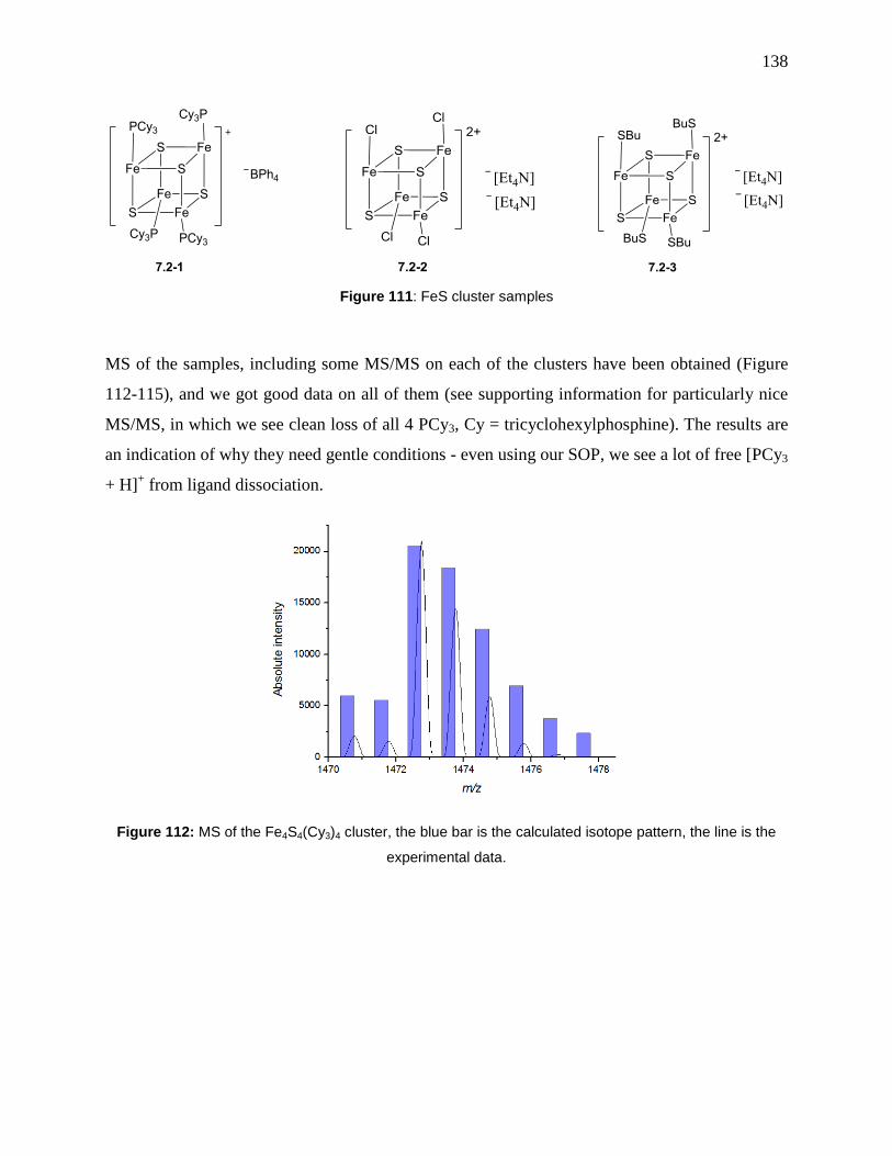
138
Figure 111: FeS cluster samples
MS of the samples, including some MS/MS on each of the clusters have been obtained (Figure
112-115), and we got good data on all of them (see supporting information for particularly nice
MS/MS, in which we see clean loss of all 4 PCy3, Cy = tricyclohexylphosphine). The results are
an indication of why they need gentle conditions - even using our SOP, we see a lot of free [PCy3
+ H]+ from ligand dissociation.
Figure 112: MS of the Fe4S4(Cy3)4 cluster, the blue bar is the calculated isotope pattern, the line is the
experimental data.

139
Figure 113: MS/MS of the 7.2-1. We can see many fragments of the mother ion-1472.9, the daughter
ions: 1192.6, 912.0, 631.9 and 351.7 are due to lose of PCy3.
Figure 114: MS/MS of the 7.2-2, 623.7 is [7.2-2 + Et4N]+, 493.5 is 7.2-2, 458.5 is [7.2-2 – Cl]
+.

140
Figure 115: MS/MS of 7.2-3, 838.0 is [7.2-2 + Et4N]
+, 618.8 is [7.2-2 - SBu]
+, 383.6 is [7.2-2 – 3*SBu]
+
The [Fe4(SBu)4]2-
dianions have more complicated spectra than the cation, because ionization
can proceed in different ways, i.e. X- loss to form [M-X]
- monoanions, and aggregation with a
cation to form [M + cation]- monoanions, as well as just the [M]
2- dianions. MS/MS were done
of the highest m/z species only. The only puzzling aspect was the appearance of additional ions
at 24 Da above the main species for the [Fe4(SBu)4]2-
cluster. This is an unusual increment, and it
probably does not mean addition of a small molecule, but rather a substitution (i.e. exchange of
SBu for something 24 Da heavier than SBu). This species remained unassigned as an unknown
impurity. This work has not yet been published.
7.3 Lactide polymerization by cationic zinc complexes
Professor Paul Hayes and coworkers from University of Lethbridge have been investigating
lactide polymerization by cationic zinc complexes.249
The air and moisture sensitive nature of
their catalysts makes it hard to identify intermediates during the polymerization process.
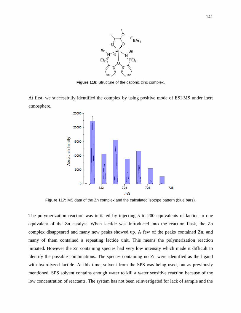
141
Figure 116: Structure of the cationic zinc complex.
At first, we successfully identified the complex by using positive mode of ESI-MS under inert
atmosphere.
Figure 117: MS data of the Zn complex and the calculated isotope pattern (blue bars).
The polymerization reaction was initiated by injecting 5 to 200 equivalents of lactide to one
equivalent of the Zn catalyst. When lactide was introduced into the reaction flask, the Zn
complex disappeared and many new peaks showed up. A few of the peaks contained Zn, and
many of them contained a repeating lactide unit. This means the polymerization reaction
initiated. However the Zn containing species had very low intensity which made it difficult to
identify the possible combinations. The species containing no Zn were identified as the ligand
with hydrolyzed lactide. At this time, solvent from the SPS was being used, but as previously
mentioned, SPS solvent contains enough water to kill a water sensitive reaction because of the
low concentration of reactants. The system has not been reinvestigated for lack of sample and the
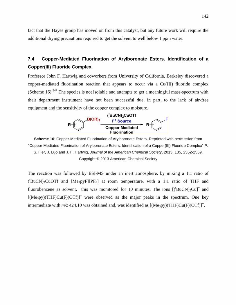
142
fact that the Hayes group has moved on from this catalyst, but any future work will require the
additional drying precautions required to get the solvent to well below 1 ppm water.
7.4 Copper-Mediated Fluorination of Arylboronate Esters. Identification of a
Copper(III) Fluoride Complex
Professor John F. Hartwig and coworkers from University of California, Berkeley discovered a
copper-mediated fluorination reaction that appears to occur via a Cu(III) fluoride complex
(Scheme 16).247
The species is not isolable and attempts to get a meaningful mass-spectrum with
their department instrument have not been successful due, in part, to the lack of air-free
equipment and the sensitivity of the copper complex to moisture.
Scheme 16: Copper-Mediated Fluorination of Arylboronate Esters. Reprinted with permission from
“Copper-Mediated Fluorination of Arylboronate Esters. Identification of a Copper(III) Fluoride Complex” P.
S. Fier, J. Luo and J. F. Hartwig, Journal of the American Chemical Society, 2013, 135, 2552-2559.
Copyright © 2013 American Chemical Society
The reaction was followed by ESI-MS under an inert atmosphere, by mixing a 1:1 ratio of
(tBuCN)2CuOTf and [Me3pyF][PF6] at room temperature, with a 1:1 ratio of THF and
fluorobenzene as solvent, this was monitored for 10 minutes. The ions [(tBuCN)2Cu]
+ and
[(Me3py)(THF)Cu(F)(OTf)]+ were observed as the major peaks in the spectrum. One key
intermediate with m/z 424.10 was obtained and, was identified as [(Me3py)(THF)Cu(F)(OTf)]+.
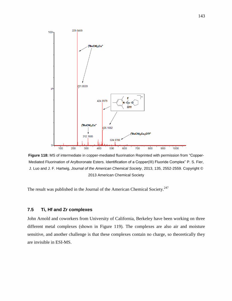
143
Figure 118: MS of intermediate in copper-mediated fluorination Reprinted with permission from “Copper-
Mediated Fluorination of Arylboronate Esters. Identification of a Copper(III) Fluoride Complex” P. S. Fier,
J. Luo and J. F. Hartwig, Journal of the American Chemical Society, 2013, 135, 2552-2559. Copyright ©
2013 American Chemical Society
The result was published in the Journal of the American Chemical Society.247
7.5 Ti, Hf and Zr complexes
John Arnold and coworkers from University of California, Berkeley have been working on three
different metal complexes (shown in Figure 119). The complexes are also air and moisture
sensitive, and another challenge is that these complexes contain no charge, so theoretically they
are invisible in ESI-MS.

144
Figure 119: Ti, Hf and Zr complexes
In order to characterize these compounds, inert atmosphere ESI-MS was used with Na[BArF
4]
with the intention that these complexes would associate with Na+ via the methoxy functionality.
By using pressurized sample vials, large Schlenk flasks could be avoided for these samples, and
these vials are disposable, eliminating cross contamination.
ESI-MS of 7-5-1 in positive mode generated a peak at m/z 867.2, 1 off from the expected m/z
868.3 for [M+Na]+ (Figure 120). For complexes 7-5-2 and 7-5-3, only the monomer was
observed instead of the dimer, suggesting that the dimer could not survive the ESI process or that
the solution did not contain dimer. The Arnold group is still comprehanding these results.
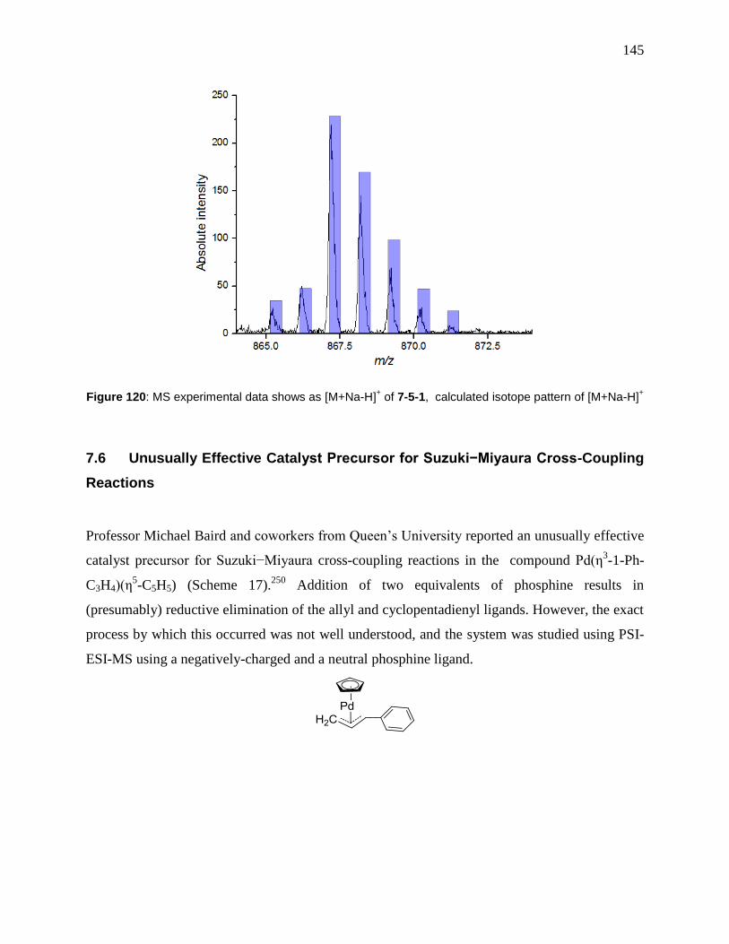
145
Figure 120: MS experimental data shows as [M+Na-H]+ of 7-5-1, calculated isotope pattern of [M+Na-H]
+
7.6 Unusually Effective Catalyst Precursor for Suzuki−Miyaura Cross-Coupling
Reactions
Professor Michael Baird and coworkers from Queen’s University reported an unusually effective
catalyst precursor for Suzuki−Miyaura cross-coupling reactions in the compound Pd(η3-1-Ph-
C3H4)(η5-C5H5) (Scheme 17).
250 Addition of two equivalents of phosphine results in
(presumably) reductive elimination of the allyl and cyclopentadienyl ligands. However, the exact
process by which this occurred was not well understood, and the system was studied using PSI-
ESI-MS using a negatively-charged and a neutral phosphine ligand.
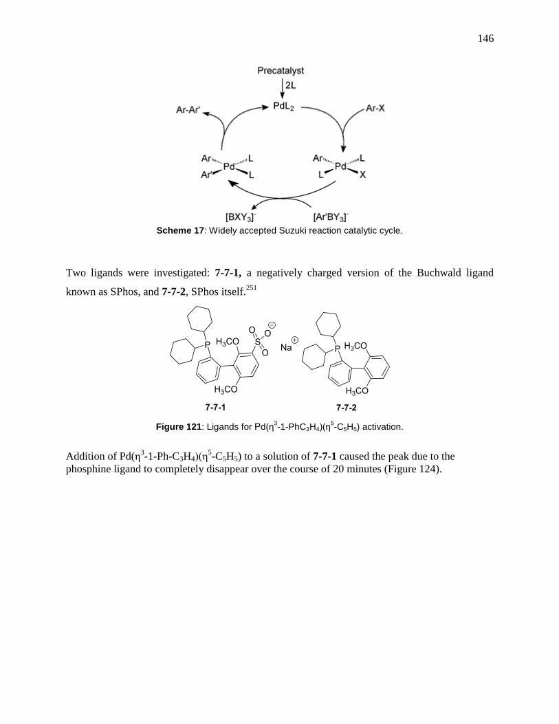
146
Scheme 17: Widely accepted Suzuki reaction catalytic cycle.
Two ligands were investigated: 7-7-1, a negatively charged version of the Buchwald ligand
known as SPhos, and 7-7-2, SPhos itself.251
Figure 121: Ligands for Pd(η3-1-PhC3H4)(η
5-C5H5) activation.
Addition of Pd(η3-1-Ph-C3H4)(η
5-C5H5) to a solution of 7-7-1 caused the peak due to the
phosphine ligand to completely disappear over the course of 20 minutes (Figure 124).

147
Figure 122: Negative mode, ESI-MS. Addition of Pd(η3-1-Ph-C3H4)(η
5-C5H5) to charged ligand 7-7-1
makes ligand disappear over the course of about 20 minutes.
The most abundant species to appear was the expected Pd(0) catalyst, [Pd(7-7-1)2]2–
(Figure
123), but its abundance was only a tiny fraction of that of the original ligand. This sort of
disappearance of charged species suggests some sort of neutralization event. Therefore the
reaction was studied again, this time with neutral Sphos, 7-7-2.
Figure 123: (7.7.1)2Pd species is the main Pd containing peak in the reaction, however the calculated
isotope pattern (blue bars) shows a extra H is present.
Addition of the neutral catalyst precursor to the neutral ligand did in fact generate charged
species: one containing Pd, the cationic allyl complex [Pd(η3-1-Ph-C3H4)(7-7-2)]
+, and the other
the allyl phosphonium compound [(C3H4)Ph (7-7-2)]+ .

148
Figure 124: In positive mode of ESI-MS. Reaction with 7-7-2 as ligand. The blue species is
[PhC3H4+7.7.2]+, the red species is [η
3-1-PhC3H4+Pd+7-7-2]
+
Formation of these complexes explains the disappearance of the anionic ligand, since both Pd(η3-
1-PhC3H4)(7-7-1) and (C3H4)Ph(7-7-1) would be zwitterionic and hence invisible to ESI-MS.
These results leave some unanswered questions: What happens to the cyclopentadienyl ligand? Is
the allyl phosphonium compound generated by reductive elimination from the Pd complex?
More work is required on this system, and we await word from Queens on the complementary
NMR experiments being conducted there. However, the initial PSI-ESI-MS results have
provided some promising insights.
7.7 Rhodium complexes catalyzed hydroacylation reaction
Professor Andrew Weller and coworkers from University of Oxford have been investigating
hydroacylation reaction catalyzed by rhodium complexes.22
By using different chelating
diphosphine ligands, the Rh complexes are efficient for reactions shown in Scheme 18. NMR
studies provided evidence of the existence of some key intermediates; however, the detailed
mechanism and the kinetic behavior studies of the reaction are still important for fully
understanding this reaction.
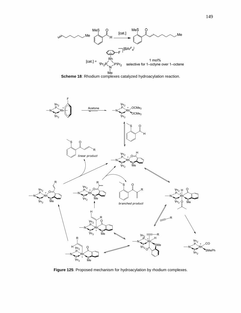
149
Scheme 18: Rhodium complexes catalyzed hydroacylation reaction.
Figure 125: Proposed mechanism for hydroacylation by rhodium complexes.
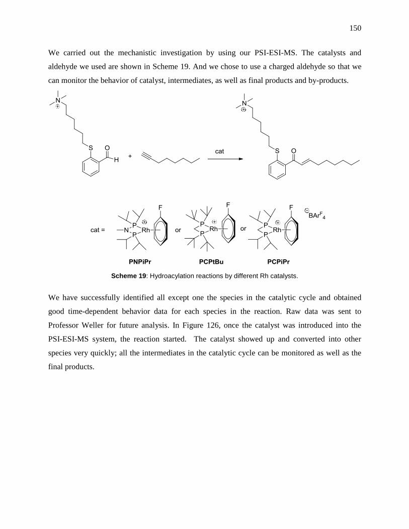
150
We carried out the mechanistic investigation by using our PSI-ESI-MS. The catalysts and
aldehyde we used are shown in Scheme 19. And we chose to use a charged aldehyde so that we
can monitor the behavior of catalyst, intermediates, as well as final products and by-products.
Scheme 19: Hydroacylation reactions by different Rh catalysts.
We have successfully identified all except one the species in the catalytic cycle and obtained
good time-dependent behavior data for each species in the reaction. Raw data was sent to
Professor Weller for future analysis. In Figure 126, once the catalyst was introduced into the
PSI-ESI-MS system, the reaction started. The catalyst showed up and converted into other
species very quickly; all the intermediates in the catalytic cycle can be monitored as well as the
final products.

151
0
0.05
0.1
0.15
0.2
0.25
0.3
0.35
0.4
0 60 120 180
0
0.05
0.1
0.15
0.2
0.25
0.3
0.35
0 60 120 180
0
0.02
0.04
0.06
0.08
0.1
0 60 120 180
0
0.02
0.04
0.06
0.08
0.1
0.12
0.14
0.16
0.18
0 60 120 180
0
0.01
0.02
0.03
0.04
0.05
0.06
0 20 40 600
0.05
0.1
0.15
0.2
0.25
0.3
0 60 120 180
Figure 126: Hydroacylation catalytic cycle with reaction online monitoring results.
All except one on cycle species in the hydroacylation catalytic cycle were identified and kinetics
data were obtained. In this figure, PCPtBu was used as catalyst, once the catalyst was introduced
in the solution, reaction started processing. The time dependent behavior of each species has
been portrayed in different colors, the color corresponds to the compounds of the same color.

152
7.8 CryoSpray MS (CSI-MS)
I was honored to win a Quebec research fellowship for 6 months of study and research in
Professor Garry Hanan’s lab at University of Montreal. There, we mainly used Bruker
MicrOTOF high resolution MS for MS related studies; recently Hanan’s group acquired the first
CryoSpray ionization (CSI) source in Canada. Coldspray Ionization was first developed by
Kentaro Yamaguchi in 2000.252
The general technique is very similar to electrospray ionization,
they have a similar ESI probe and desolvation chamber. CSI is a very soft ionization technique;
it is even “softer” than ESI. It can solve the problem of decomposition of fragile compounds
induced by high temperature during the ESI desolvation process. By using low temperature spray
cone gas and drying gas, CSI can cool the source and desolvation chamber to reduce
decomposition.
CSI-MS is a good technique for studying weak-interaction chemistry such as multiple charged
and highly solvated ions; labile organic and organometallic complexes, DNA di-/tri-/quadru-
plexs, and hyper-stranded DNAs.253
With CSI, we have successfully characterized over 80 weak non-covalent bonding
supramolecular complexes, examples are shown below.
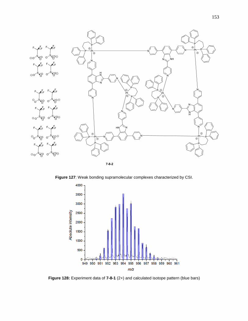
153
Figure 127: Weak bonding supramolecular complexes characterized by CSI.
Figure 128: Experiment data of 7-8-1 (2+) and calculated isotope pattern (blue bars)
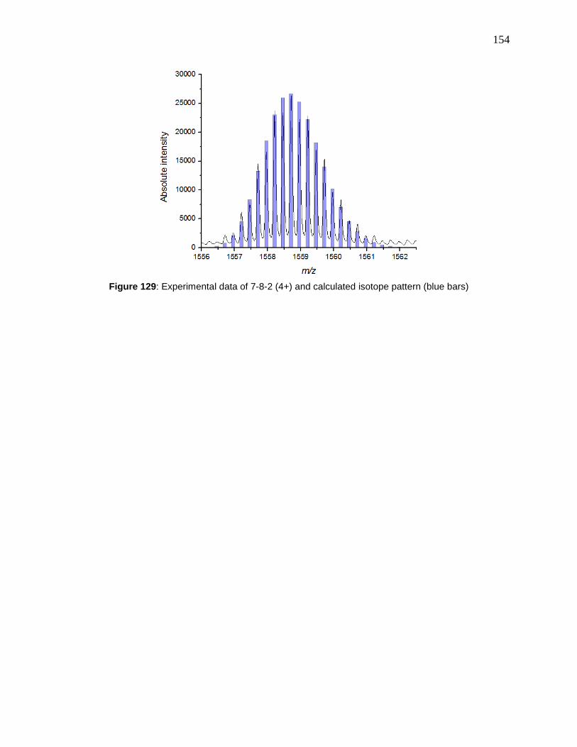
154
Figure 129: Experimental data of 7-8-2 (4+) and calculated isotope pattern (blue bars)

155
8. Conclusion
The work presented here describes the ongoing development and application of pressurized
sample infusion (PSI) in catalysis reaction studies. Since the invention of the PSI-ESI-MS, the
technique has been used on various projects.
Chapter one and two serve as an introduction to ESI-MS and organometallic catalysis. In chapter
three, the optimization of pressurized sample infusion was discussed. In chapter four, we applied
PSI to an intramolecular Pauson-Khand reaction; it is the first PSI-ESI-MS experiment to have
been done with a reactive gas (CO) rather than protective gas such as N2 and Ar. We overcame
solubility problems by using a second solvent as a dilution solvent. This reaction was also the
first time PSI-ESI-MS has been used for entropy and enthalpy calculations. We have
demonstrated that PSI-ESI-MS is a powerful technique to study the Pauson-Khand reaction. A
CO dissociation was confirmed as rate limiting step in the catalytic cycle.
In chapter five, we used H2 gas for Rh-catalyzed hydrogenation kinetic studies. Conventional
Wilkinson’s catalyst was used and, for comparison, the more reactive Rh-based “Weller’s
catalyst” was also used. The two catalysts behave very differently in terms of hydrogenation.
“Weller’s catalyst” is capable of semi-hydrogenation as concluded from the PSI-ESI-MS results.
Numerical modeling was integrated with PSI-ESI-MS, and calculated data matches the
experimental data perfectly. In chapter six, where PSI was used for catalytic Si-H activation
reaction studies, we were able to gain a deeper understanding of reactions such as
dehydrocoupling of silanes and alcoholization of silane. However, since these are such
complicated reactions, more work should be done in future including the use of lower reactivity
secondary silanes for the dehydrocoupling of silanes and the use of different alcohols and
reaction conditions for alcoholization of silanes.
Finally, in the past five years, over ten collaborative projects from different research institutes
and industries have been carried out by using PSI technique. Good results were obtained, and
many optimizations have been added to the PSI technique.
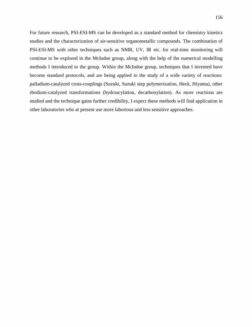
156
For future research, PSI-ESI-MS can be developed as a standard method for chemistry kinetics
studies and the characterization of air-sensitive organometallic compounds. The combination of
PSI-ESI-MS with other techniques such as NMR, UV, IR etc. for real-time monitoring will
continue to be explored in the McIndoe group, along with the help of the numerical modelling
methods I introduced to the group. Within the McIndoe group, techniques that I invented have
become standard protocols, and are being applied in the study of a wide variety of reactions:
palladium-catalyzed cross-couplings (Suzuki, Suzuki step polymerization, Heck, Hiyama), other
rhodium-catalyzed transformations (hydroacylation, decarbonylation). As more reactions are
studied and the technique gains further credibility, I expect these methods will find application in
other laboratories who at present use more laborious and less sensitive approaches.
157
References
1. P. T. Anastas and J. C. Warner, Green Chemistry: Theory and Practice, Oxford University Press,
Incorporated, 1998. 2. M. Schlosser and L. S. Hegedus, Organometallics in synthesis : a manual, J. Wiley, Chichester;
New York [etc.], 1994. 3. D. Astruc, Organometallic chemistry and catalysis, Springer, Berlin ; New York, 2007. 4. R. H. Crabtree, The organometallic chemistry of the transition metals, John Wiley, 2001. 5. E. V. Gusevskaya, Quim. Nova, 2003, 26, 242-248. 6. http://www.nobelprize.org/nobel_prizes/chemistry/laureates/2005/, Accessed April 23, 2014. 7. P. Jean-Louis Hérisson and Y. Chauvin, Die Makromolekulare Chemie, 1971, 141, 161-176. 8. http://www.nobelprize.org/nobel_prizes/chemistry/laureates/2005/advanced.html, Accessed
Dec 5, 2013. 9. http://www.nobelprize.org/nobel_prizes/chemistry/laureates/2010/, Accessed April 23, 2014. 10. R. F. Heck, J. Am. Chem. Soc., 1969, 91, 6707-6714. 11. M. Bradshaw, J. Zou, L. Byrne, K. Swaminathan Iyer, S. G. Stewart and C. L. Raston, Chem.
Commun. (Cambridge, U. K.), 2011, 47, 12292-12294. 12. F. Ozawa, A. Kubo and T. Hayashi, Chem. Lett., 1992, 21, 2177-2180. 13. A. O. King, N. Okukado and E.-i. Negishi, J. Chem. Soc., Chem. Commun., 1977, 683-684. 14. N. Miyaura, K. Yamada and A. Suzuki, Tetrahedron Lett., 1979, 20, 3437-3440. 15. http://en.wikipedia.org/wiki/Nuclear_magnetic_resonance_spectroscopy, Accessed May 15,
2014. 16. S. M. Jackson, D. M. Chisholm, J. S. McIndoe and L. Rosenberg, Eur. J. Inorg. Chem., 2011, 2011,
327-330. 17. C. Godard, S. B. Duckett, S. Polas, R. Tooze and A. C. Whitwood, Dalton Trans., 2009, 2496-2509. 18. C. Zuccaccia, G. Bellachioma, S. Bolaño, L. Rocchigiani, A. Savini and A. Macchioni, Eur. J. Inorg.
Chem., 2012, 2012, 1462-1468. 19. S. Mom, M. Beaupérin, D. Roy, S. Royer, R. Amardeil, H. Cattey, H. Doucet and J. C. Hierso, Inorg.
Chem., 2011, 50, 11592-11603. 20. M. Boutain, S. B. Duckett, J. P. Dunne, C. Godard, J. M. Hernandez, A. J. Holmes, I. G. Khazal and
J. Lopez-Serrano, Dalton Trans., 2010, 39, 3495-3500. 21. D. J. Darensbourg, S. J. Kyran, A. D. Yeung and A. A. Bengali, Eur. J. Inorg. Chem., 2013, 2013,
4024-4031. 22. I. Pernik, J. F. Hooper, A. B. Chaplin, A. S. Weller and M. C. Willis, ACS Catalysis, 2012, 2, 2779-
2786. 23. J. M. Larsson and K. J. Szabó, J. Am. Chem. Soc., 2012, 135, 443-455. 24. D. A. Skoog, F. J. Holler and S. R. Crouch, Principles of instrumental analysis, Thomson
Brooks/Cole, 2007. 25. C. Fischer, T. Beweries, A. Preetz, H.-J. Drexler, W. Baumann, S. Peitz, U. Rosenthal and D. Heller,
Catal. Today, 2010, 155, 282-288. 26. F. Gao, M. B. Sullivan, G. M. Kuramshina, L. Guo and M. Garland, ChemPhysChem, 2012, 13,
3139-3145. 27. C. A. Jaska and I. Manners, J. Am. Chem. Soc., 2004, 126, 9776-9785. 28. M. Bauer, T. Kauf, J. Christoffers and H. Bertagnolli, Phys. Chem. Chem. Phys., 2005, 7, 2664-
2670. 29. M. V. Joshi, S. Vaidya, R. Pandey and D. Mukesh, J. Catal., 1999, 183, 102-106.
158
30. C. Amatore and A. Jutand, J. Organomet. Chem., 1999, 576, 254-278. 31. N. Matyasovszky, M. Tian and A. Chen, The Journal of Physical Chemistry A, 2009, 113, 9348-
9353. 32. H. Maskill, The Investigation of Organic Reactions and Their Mechanisms, Wiley, 2008. 33. S. Sarkar, S. Niyogi, E. Bekyarova and R. C. Haddon, Chemical Science, 2011, 2, 1326-1333. 34. T. Zhang, W. Li and J.-P. Croue, Environ. Sci. Technol., 2011. 35. L. Bini, E. J. E. Houben, E. A. Pidko, C. Müller and D. Vogt, Catal. Today, 2010, 155, 271-278. 36. http://us.mt.com/us/en/home/products/L1_AutochemProducts/L2_in-situSpectrocopy.html,
Accessed Oct 26, 2011. 37. G. Barker, J. L. McGrath, A. Klapars, D. Stead, G. Zhou, K. R. Campos and P. O’Brien, The Journal
of Organic Chemistry, 2011, 76, 5936-5953. 38. E. Le Gall, S. Sengmany, C. Hauréna, E. Léonel and T. Martens, J. Organomet. Chem., 2013, 736,
27-35. 39. W. Henderson and J. S. McIndoe, Mass spectrometry of inorganic and organometallic
compounds, J. Wiley, 2005. 40. M. N. Eberlin, Eur. J. Mass Spectrom., 2007, 13, 19-28. 41. R. B. Cole, Electrospray and MALDI Mass Spectrometry: Fundamentals, Instrumentation,
Practicalities, and Biological Applications, John Wiley & Sons, 2009. 42. http://www.magnet.fsu.edu/education/tutorials/tools/ionization_esi.html, Accessed Oct 07,
2011. 43. L. S. Santos, Reactive Intermediates: MS Investigations in Solution, Wiley-VCH, 2010. 44. M. Bonchio, G. Licini, G. Modena, O. Bortolini, S. Moro and W. A. Nugent, J. Am. Chem. Soc.,
1999, 121, 6258-6268. 45. Z. Li, Z. H. Tang, X. X. Hu and C. G. Xia, Chemistry – A European Journal, 2005, 11, 1210-1216. 46. B. C. Gilbert, J. R. Lindsay Smith, A. Mairata i Payeras, J. Oakes and R. Pons i Prats, J. Mol. Catal.
A: Chem., 2004, 219, 265-272. 47. K. L. Vikse, Z. Ahmadi, C. C. Manning, D. A. Harrington and J. S. McIndoe, Angewandte Chemie
International Edition, 2011, 50, 8304-8306. 48. F. Wu, S. R. Foley, C. T. Burns and R. F. Jordan, J. Am. Chem. Soc., 2005, 127, 1841-1853. 49. L. S. Santos, Eur. J. Org. Chem., 2008, 2008, 235-253. 50. M. A. Henderson, J. Luo, A. Oliver and J. S. McIndoe, Organometallics, 2011. 51. C. Adlhart and P. Chen, Helv. Chim. Acta, 2003, 86, 941-949. 52. Y.-M. Kim and P. Chen, Int. J. Mass Spectrom., 1999, 185–187, 871-881. 53. C. Hinderling, C. Adlhart and P. Chen, Angewandte Chemie International Edition, 1998, 37, 2685-
2689. 54. D. Feichtinger, D. A. Plattner and P. Chen, J. Am. Chem. Soc., 1998, 120, 7125-7126. 55. P. Chen, Angewandte Chemie International Edition, 2003, 42, 2832-2847. 56. M. Eberlin, Eur. J. Mass Spectrom., 2007, 13, 19-28. 57. J. A. Lessa, A. Horn, É. S. Bull, M. R. Rocha, M. Benassi, R. R. Catharino, M. N. Eberlin, A.
Casellato, C. J. Noble, G. R. Hanson, G. Schenk, G. C. Silva, O. A. C. Antunes and C. Fernandes, Inorg. Chem., 2009, 48, 4569-4579.
58. L. S. Santos, C. H. Pavam, W. P. Almeida, F. Coelho and M. N. Eberlin, Angewandte Chemie International Edition, 2004, 43, 4330-4333.
59. Y. Blum, D. Czarkie, Y. Rahamim and Y. Shvo, Organometallics, 1985, 4, 1459-1461. 60. B. G. Vaz, C. D. F. Milagre, M. N. Eberlin and H. M. S. Milagre, Org. Biomol. Chem., 2013, 11,
6695-6698. 61. L. Taghizadeh Ghoochany, C. Kerner, S. Farsadpour, F. Menges, Y. Sun, G. Niedner-Schatteburg
and W. R. Thiel, Eur. J. Inorg. Chem., 2013, 2013, 4305-4317.

159
62. A. H. L. Machado, H. M. S. Milagre, L. S. Eberlin, A. A. Sabino, C. R. D. Correia and M. N. Eberlin, Org. Biomol. Chem., 2013, 11, 3277-3281.
63. T. K. Trefz, M. A. Henderson, M. Y. Wang, S. Collins and J. S. McIndoe, Organometallics, 2013, 32, 3149-3152.
64. M. Parera, A. Dachs, M. Solà, A. Pla-Quintana and A. Roglans, Chemistry – A European Journal, 2012, 18, 13097-13107.
65. J. Griffiths, Anal. Chem., 2008, 80, 5678-5683. 66. A. Dempster, Philosophical magazine (London, England : 1945), 1916, 31, 438. 67. M. S. B. Munson and F. H. Field, J. Am. Chem. Soc., 1966, 88, 2621-2630. 68. A. G. Harrison, Chemical Ionization Mass Spectrometry, Second Edition, Taylor & Francis, 1992. 69. H. D. Beckey, International Journal of Mass Spectrometry and Ion Physics, 1969, 2, 500-502. 70. H. R. Morris, M. Panico, M. Barber, R. S. Bordoli, R. D. Sedgwick and A. Tyler, Biochem. Biophys.
Res. Commun., 1981, 101, 623-631. 71. M. Barber, R. S. Bordoli, R. D. Sedgwick and A. N. Tyler, J. Chem. Soc., Chem. Commun., 1981,
325-327. 72. D. I. Carroll, I. Dzidic, R. N. Stillwell, K. D. Haegele and E. C. Horning, Anal. Chem., 1975, 47, 2369-
2373. 73. M. Yamashita and J. B. Fenn, The Journal of Physical Chemistry, 1984, 88, 4451-4459. 74. J. B. Fenn, M. Mann, M. Chin-kai, W. Shek-fu and C. M. Whitehouse, Science, 1989, 246, 64. 75. K. Tanaka, H. Waki, Y. Ido, S. Akita, Y. Yoshida, T. Yoshida and T. Matsuo, Rapid Commun. Mass
Spectrom., 1988, 2, 151-153. 76. F. Hillenkamp and M. Karas, Int. J. Mass Spectrom., 2000, 200, 71-77. 77. L. A. McDonnell and R. M. A. Heeren, Mass Spectrom. Rev., 2007, 26, 606-643. 78. P. Chaurand, J. L. Norris, D. S. Cornett, J. A. Mobley and R. M. Caprioli, J. Proteome Res., 2006, 5,
2889-2900. 79. R. M. Caprioli, T. B. Farmer and J. Gile, Anal. Chem., 1997, 69, 4751-4760. 80. M. D. Eelman, J. M. Blacquiere, M. M. Moriarty and D. E. Fogg, Angewandte Chemie
International Edition, 2008, 47, 303-306. 81. M. Dole, L. L. Mack, R. L. Hines, R. C. Mobley, L. D. Ferguson and M. B. Alice, The Journal of
Chemical Physics, 1968, 49, 2240-2249. 82. International Journal of Analytical Chemistry, 2012, 2012. 83. R. B. Cole, J. Mass Spectrom., 2000, 35, 763-772. 84. G. Taylor, Proceedings of the Royal Society of London. Series A. Mathematical and Physical
Sciences, 1964, 280, 383-397. 85. D. C. Taflin, T. L. Ward and E. J. Davis, Langmuir, 1989, 5, 376-384. 86. L. Konermann, E. Ahadi, A. D. Rodriguez and S. Vahidi, Anal. Chem., 2012, 85, 2-9. 87. W. Corporation, Micromass Q-Tof micro Mass Spectrometer Operator’s Guide, Milford, MA, USA,
2002. 88. A. A. Nazarov, M. Baquié, P. Nowak-Sliwinska, O. Zava, J. R. van Beijnum, M. Groessl, D. M.
Chisholm, Z. Ahmadi, J. S. McIndoe, A. W. Griffioen, H. van den Bergh and P. J. Dyson, Sci. Rep., 2013, 3.
89. K. L. Vikse, M. P. Woods and J. S. McIndoe, Organometallics, 2010, 29, 6615-6618. 90. K. L. Vikse, Z. Ahmadi, J. Luo, N. van der Wal, K. Daze, N. Taylor and J. S. McIndoe, Int. J. Mass
Spectrom., 2012, 323–324, 8-13. 91. S. P. Sutera and R. Skalak, Annual Review of Fluid Mechanics, 1993, 25, 1-19. 92. P. S. Academic, Powersim Software AS, Bergen, Norway, 9 edn., 2012. 93. S. Hoops, S. Sahle, R. Gauges, C. Lee, J. Pahle, N. Simus, M. Singhal, L. Xu, P. Mendes and U.
Kummer, Bioinformatics, 2006, 22, 3067-3074.

160
94. R. Hartmann and P. Chen, Adv. Synth. Catal., 2003, 345, 1353-1359. 95. J. Luo, A. G. Oliver and J. Scott McIndoe, Dalton Trans., 2013, 42, 11312-11318. 96. Z. Ahmadi and J. S. McIndoe, Chem. Commun. (Cambridge, U. K.), 2013, 49, 11488-11490. 97. I. U. Khand, G. R. Knox, P. L. Pauson and W. E. Watts, Journal of the Chemical Society D: Chemical
Communications, 1971, 36a-36a. 98. I. U. Khand, G. R. Knox, P. L. Pauson and W. E. Watts, Journal of the Chemical Society, Perkin
Transactions 1, 1973, 975-977. 99. P. Magnus, L. M. Principe and M. J. Slater, The Journal of Organic Chemistry, 1987, 52, 1483-
1486. 100. J. Blanco-Urgoiti, L. Anorbe, L. Perez-Serrano, G. Dominguez and J. Perez-Castells, Chem. Soc.
Rev., 2004, 33, 32-42. 101. A. J. Fletcher and S. D. R. Christie, Journal of the Chemical Society, Perkin Transactions 1, 2000,
1657-1668. 102. O. Geis and H.-G. Schmalz, Angewandte Chemie International Edition, 1998, 37, 911-914. 103. T. Sugihara, M. Yamada, H. Ban, M. Yamaguchi and C. Kaneko, Angewandte Chemie International
Edition in English, 1997, 36, 2801-2804. 104. T. Sugihara, M. Yamada, M. Yamaguchi and M. Nishizawa, Synlett, 1999, 6, 771-773. 105. D. C. Billington, I. Malcolm Helps, P. L. Pauson, W. Thomson and D. Willison, J. Organomet.
Chem., 1988, 354, 233-242. 106. T. Sugihara and M. Yamaguchi, Synlett, 1998, 1998, 1384-1386. 107. K. H. Park, I. G. Jung and Y. K. Chung, Org. Lett., 2004, 6, 1183-1186. 108. N. Jeong, B. K. Sung and Y. K. Choi, J. Am. Chem. Soc., 2000, 122, 6771-6772. 109. T. Shibata, N. Toshida and K. Takagi, Org. Lett., 2002, 4, 1619-1621. 110. T. Morimoto, K. Fuji, K. Tsutsumi and K. Kakiuchi, J. Am. Chem. Soc., 2002, 124, 3806-3807. 111. K. H. Park, S. U. Son and Y. K. Chung, Chem. Commun. (Cambridge, U. K.), 2003, 1898-1899. 112. C. Mukai, M. Uchiyama and M. Hanaoka, J. Chem. Soc., Chem. Commun., 1992, 1014-1015. 113. T. Shibata and K. Takagi, J. Am. Chem. Soc., 2000, 122, 9852-9853. 114. F. A. Hicks, N. M. Kablaoui and S. L. Buchwald, J. Am. Chem. Soc., 1996, 118, 9450-9451. 115. F. A. Hicks, N. M. Kablaoui and S. L. Buchwald, J. Am. Chem. Soc., 1999, 121, 5881-5898. 116. P. Mastrorilli, C. F. Nobile, R. Paolillo and G. P. Suranna, J. Mol. Catal. A: Chem., 2004, 214, 103-
106. 117. P. Magnus, C. Exon and P. Albaugh-Robertson, Tetrahedron, 1985, 41, 5861-5869. 118. V. Rautenstrauch, P. Mégard, J. Conesa and W. Küster, Angewandte Chemie International Edition
in English, 1990, 29, 1413-1416. 119. M. Yamanaka and E. Nakamura, J. Am. Chem. Soc., 2001, 123, 1703-1708. 120. M. A. Bennett and P. B. Donaldson, Inorg. Chem., 1978, 17, 1995-2000. 121. C. M. Gordon, M. Kiszka, I. R. Dunkin, W. J. Kerr, J. S. Scott and J. Gebicki, J. Organomet. Chem.,
1998, 554, 147-154. 122. E. V. Banide, H. Müller-Bunz, A. R. Manning, P. Evans and M. J. McGlinchey, Angewandte Chemie
International Edition, 2007, 46, 2907-2910. 123. M. K. Pallerla, G. P. A. Yap and J. M. Fox, The Journal of Organic Chemistry, 2008, 73, 6137-6141. 124. T. J. M. de Bruin, A. Milet, A. E. Greene and Y. Gimbert, The Journal of Organic Chemistry, 2004,
69, 1075-1080. 125. X. Verdaguer, J. Vázquez, G. Fuster, V. Bernardes-Génisson, A. E. Greene, A. Moyano, M. A.
Pericàs and A. Riera, The Journal of Organic Chemistry, 1998, 63, 7037-7052. 126. R. Cabot, A. Lledó, M. Revés, A. Riera and X. Verdaguer, Organometallics, 2007, 26, 1134-1142. 127. D. G. Blackmond, Angewandte Chemie International Edition, 2005, 44, 4302-4320. 128. M. A. Henderson, Ph.D., Univerisity of Victoria, 2009.
161
129. W. Henderson and C. Evans, Inorg. Chim. Acta, 1999, 294, 183-192. 130. C. Decker, W. Henderson and B. K. Nicholson, Journal of the Chemical Society, Dalton
Transactions, 1999, 3507-3513. 131. N. J. Farrer, R. McDonald and J. S. McIndoe, Dalton Trans., 2006, 4570-4579. 132. N. J. Farrer, R. McDonald, T. Piga and J. S. McIndoe, Polyhedron, 2010, 29, 254-261. 133. W. Henderson and B. K. Nicholson, J. Chem. Soc., Chem. Commun., 1995, 2531-2532. 134. L. S. Santos, G. B. Rosso, R. A. Pilli and M. N. Eberlin, The Journal of Organic Chemistry, 2007, 72,
5809-5812. 135. D. M. Chisholm, A. G. Oliver and J. S. McIndoe, Dalton Trans., 2010, 39, 364-373. 136. C. Adlhart and P. Chen, Helv. Chim. Acta, 2000, 83, 2192-2196. 137. E. Crawford, T. Lohr, E. M. Leitao, S. Kwok and J. S. McIndoe, Dalton Trans., 2009, 9110-9112. 138. Y. Gimbert, D. Lesage, A. Milet, F. Fournier, A. E. Greene and J.-C. Tabet, Org. Lett., 2003, 5,
4073-4075. 139. A. D. Allian, M. Tjahjono and M. Garland, Organometallics, 2006, 25, 2182-2188. 140. M. Henderson, S. Kwok and J. S. McIndoe, J. Am. Soc. Mass Spectrom., 2009, 20, 658-666. 141. V. De Vynck and E. J. Goethals, Macromol. Rapid Commun., 1997, 18, 149-156. 142. B. R. James, Homogeneous Hydrogenation, Wiley, 1973. 143. J. F. Young, J. A. Osborn, F. H. Jardine and G. Wilkinson, Chemical Communications (London),
1965, 131-132. 144. M. A. L. Bennett, P. A., Chem. Ind. (London), 1965, 846. 145. Coffey R.S.; British Patent No.1121642, 1965. 146. J. Halpern, T. Okamoto and A. Zakhariev, J. Mol. Catal., 1977, 2, 65-68. 147. M. I. Cabrera, P. D. Zgolicz and R. J. Grau, Applied Catalysis A: General, 2008, 334, 291-303. 148. D. J. Nelson, R. Li and C. Brammer, The Journal of Organic Chemistry, 2004, 70, 761-767. 149. M. Bowker, J. Gland, R. Joyner, Y. Li, M. Slin'ko and R. Whyman, Catal. Lett., 1994, 25, 293-308. 150. N. Koga, C. Daniel, J. Han, X. Y. Fu and K. Morokuma, J. Am. Chem. Soc., 1987, 109, 3455-3456. 151. D. Wink and P. C. Ford, J. Am. Chem. Soc., 1985, 107, 1794-1796. 152. D. A. Wink and P. C. Ford, J. Am. Chem. Soc., 1987, 109, 436-442. 153. S. B. Duckett, C. L. Newell and R. Eisenberg, J. Am. Chem. Soc., 1993, 115, 1156-1157. 154. S. B. Duckett, C. L. Newell and R. Eisenberg, J. Am. Chem. Soc., 1994, 116, 10548-10556. 155. I. V. Koptyug, K. V. Kovtunov, S. R. Burt, M. S. Anwar, C. Hilty, S.-I. Han, A. Pines and R. Z.
Sagdeev, J. Am. Chem. Soc., 2007, 129, 5580-5586. 156. J. Halpern, Inorg. Chim. Acta, 1981, 50, 11-19. 157. D. Chisholm, Ph.D., Univerisity of Victoria, 2010. 158. P. J. Dyson, J. S. McIndoe and D. Zhao, Chem. Commun. (Cambridge, U. K.), 2003, 508-509. 159. D. M. Chisholm and J. Scott McIndoe, Dalton Trans., 2008, 3933-3945. 160. T. Müller, A. Badu-Tawiah and R. G. Cooks, Angewandte Chemie International Edition, 2012, 51,
11832-11835. 161. Powersim Software AS, Bergen, Norway, 9 edn., 2012. 162. C. A. Tolman, P. Z. Meakin, D. I. Lindner and J. P. Jesson, J. Am. Chem. Soc., 1974, 96, 2762-2774. 163. P. Meakin, J. P. Jesson and C. A. Tolman, J. Am. Chem. Soc., 1972, 94, 3240-3242. 164. M. Armbrüster, M. Behrens, F. Cinquini, K. Föttinger, Y. Grin, A. Haghofer, B. Klötzer, A. Knop-
Gericke, H. Lorenz, A. Ota, S. Penner, J. Prinz, C. Rameshan, Z. Révay, D. Rosenthal, G. Rupprechter, P. Sautet, R. Schlögl, L. Shao, L. Szentmiklósi, D. Teschner, D. Torres, R. Wagner, R. Widmer and G. Wowsnick, ChemCatChem, 2012, 4, 1048-1063.
165. M. P. R. Spee, J. Boersma, M. D. Meijer, M. Q. Slagt, G. van Koten and J. W. Geus, The Journal of Organic Chemistry, 2001, 66, 1647-1656.
166. I. N. Michaelides and D. J. Dixon, Angewandte Chemie International Edition, 2013, 52, 806-808.

162
167. M. Yan, T. Jin, Y. Ishikawa, T. Minato, T. Fujita, L.-Y. Chen, M. Bao, N. Asao, M.-W. Chen and Y. Yamamoto, J. Am. Chem. Soc., 2012, 134, 17536-17542.
168. K. Urabe, Y. Tanaka and Y. Izumi, Chem. Lett., 1985, 14, 1595-1596. 169. R. R. Schrock and J. A. Osborn, J. Am. Chem. Soc., 1976, 98, 2143-2147. 170. L. J. Sewell, G. C. Lloyd-Jones and A. S. Weller, J. Am. Chem. Soc., 2012, 134, 3598-3610. 171. B. R. James and D. Mahajan, Can. J. Chem., 1979, 57, 180-187. 172. M. A. Esteruelas, I. González, J. Herrero and L. A. Oro, J. Organomet. Chem., 1998, 551, 49-53. 173. C. Kohrt, G. Wienhöfer, C. Pribbenow, M. Beller and D. Heller, ChemCatChem, 2013, 5, 2818-
2821. 174. B. R. James and D. K. W. Wang, Can. J. Chem., 1980, 58, 245-250. 175. W. S. Knowles, Adv. Synth. Catal., 2003, 345, 3-13. 176. J. Cipot, R. McDonald, M. J. Ferguson, G. Schatte and M. Stradiotto, Organometallics, 2007, 26,
594-608. 177. S. Bell, B. Wüstenberg, S. Kaiser, F. Menges, T. Netscher and A. Pfaltz, Science, 2006, 311, 642-
644. 178. C. J. Longley, T. J. Goodwin and G. Wilkinson, Polyhedron, 1986, 5, 1625-1628. 179. B. R. James, Catal. Today, 1997, 37, 209-221. 180. S. Kobayashi and H. Ishitani, Chem. Rev. (Washington, DC, U. S.), 1999, 99, 1069-1094. 181. S. Doran, T. Achard, A. Riera and X. Verdaguer, J. Organomet. Chem., 2012, 717, 135-140. 182. V. Cadierno, J. Díez, S. E. García-Garrido, J. Gimeno and A. Pizzano, Polyhedron, 2010, 29, 3380-
3386. 183. M. Ahlquist, M. Gustafsson, M. Karlsson, M. Thaning, O. Axelsson and O. F. Wendt, Inorg. Chim.
Acta, 2007, 360, 1621-1627. 184. M. J. Burk, T. G. P. Harper, J. R. Lee and C. Kalberg, Tetrahedron Lett., 1994, 35, 4963-4966. 185. W. H. Bernskoetter, E. Lobkovsky and P. J. Chirik, J. Am. Chem. Soc., 2005, 127, 14051-14061. 186. K. E. Janak and G. Parkin, J. Am. Chem. Soc., 2003, 125, 13219-13224. 187. J. F. Hooper, R. D. Young, A. S. Weller and M. C. Willis, Chemistry – A European Journal, 2013, 19,
3125-3130. 188. J. B. Lambert and L. G. Greifenstein, J. Am. Chem. Soc., 1974, 96, 5120-5124. 189. H. Yang, H. Gao and R. J. Angelici, Organometallics, 1999, 18, 2285-2287. 190. J. Blum, A. Rosenfeld, F. Gelman, H. Schumann and D. Avnir, J. Mol. Catal. A: Chem., 1999, 146,
117-122. 191. M. S. Hill, ChemInform, 2011, 42, no-no. 192. D. J. Harrison, D. R. Edwards, R. McDonald and L. Rosenberg, Dalton Transactions, 2008, 3401-
3411. 193. R. D. Miller and J. Michl, Chemical Reviews, 1989, 89, 1359-1410. 194. J. F. Harrod and S. S. Yun, Organometallics, 1987, 6, 1381-1387. 195. C. Aitken, J. F. Harrod and E. Samuel, Journal of Organometallic Chemistry, 1985, 279, C11-C13. 196. B.-H. Kim, H.-G. Woo, W. Kim and H. Li, Journal of Chemical Technology & Biotechnology, 2006,
81, 782-788. 197. H. G. Woo, J. F. Walzer and T. D. Tilley, Journal of the American Chemical Society, 1992, 114,
7047-7055. 198. J. J. Chruściel, Canadian Journal of Chemistry, 2005, 83, 508-516. 199. P. Diversi, F. Marchetti, V. Ermini and S. Matteoni, Journal of Organometallic Chemistry, 2000,
593-594, 154-160. 200. M. Itazaki, K. Ueda and H. Nakazawa, Angewandte Chemie International Edition, 2009, 48, 3313-
3316. 201. E. E. Smith, G. Du, P. E. Fanwick and M. M. Abu-Omar, Organometallics, 2010, 29, 6527-6533.
163
202. S. M. Jackson, C. E. Hughes, S. Monfette and L. Rosenberg, Inorganica Chimica Acta, 2006, 359, 2966-2972.
203. S. M. Jackson, University of Victoria Dept of Chemistry University of Victoria, 2007. 204. D. M. Hester, J. Sun, A. W. Harper and G. K. Yang, Journal of the American Chemical Society,
1992, 114, 5234-5240. 205. G. P. Mitchell and T. D. Tilley, Organometallics, 1996, 15, 3477-3479. 206. G. P. Mitchell and T. D. Tilley, Organometallics, 1998, 17, 2912-2916. 207. I. Ojima, S.-I. Inaba, T. Kogure and Y. Nagai, Journal of Organometallic Chemistry, 1973, 55, C7-
C8. 208. L. Rosenberg, C. W. Davis and J. Yao, Journal of the American Chemical Society, 2001, 123, 5120-
5121. 209. K. Mori, M. Tano, T. Mizugaki, K. Ebitani and K. Kaneda, New Journal of Chemistry, 2002, 26,
1536-1538. 210. http://www.acmite.com/market-reports/chemicals/world-silicone-market.html, Accessed
March 5, 2014. 211. M. A. Brook, Silicon in organic, organometallic, and polymer chemistry, J. Wiley, 2000. 212. N. Asao, Y. Ishikawa, N. Hatakeyama, Menggenbateer, Y. Yamamoto, M. Chen, W. Zhang and A.
Inoue, Angewandte Chemie International Edition, 2010, 49, 10093-10095. 213. M. Lee, S. Ko and S. Chang, J. Am. Chem. Soc., 2000, 122, 12011-12012. 214. S. T. Tan, J. W. Kee and W. Y. Fan, Organometallics, 2011, 30, 4008-4013. 215. T. Y. Lee, L. Dang, Z. Zhou, C. H. Yeung, Z. Lin and C. P. Lau, Eur. J. Inorg. Chem., 2010, 2010,
5675-5684. 216. B. P. S. Chauhan, A. Sarkar, M. Chauhan and A. Roka, Appl. Organomet. Chem., 2009, 23, 385-
390. 217. T. Mitsudome, S. Arita, H. Mori, T. Mizugaki, K. Jitsukawa and K. Kaneda, Angewandte Chemie
International Edition, 2008, 47, 7938-7940. 218. T. Mitsudome, A. Noujima, T. Mizugaki, K. Jitsukawa and K. Kaneda, Chemical Communications,
2009, 5302-5304. 219. R. A. Corbin, E. A. Ison and M. M. Abu-Omar, Dalton Trans., 2009, 2850-2855. 220. E. A. Ison, R. A. Corbin and M. M. Abu-Omar, J. Am. Chem. Soc., 2005, 127, 11938-11939. 221. Y. Lee, D. Seomoon, S. Kim, H. Han, S. Chang and P. H. Lee, The Journal of Organic Chemistry,
2004, 69, 1741-1743. 222. T. Mitsudome, A. Noujima, T. Mizugaki, K. Jitsukawa and K. Kaneda, Chem. Commun.
(Cambridge, U. K.), 2009, 5302-5304. 223. R. Aroop K, in Advances in Organometallic Chemistry, eds. A. F. H. Robert West and J. F. Mark,
Academic Press, 2007, vol. Volume 55, pp. 1-59. 224. S. C. Bart, E. Lobkovsky and P. J. Chirik, Journal of the American Chemical Society, 2004, 126,
13794-13807. 225. J. Stein, L. N. Lewis, Y. Gao and R. A. Scott, J. Am. Chem. Soc., 1999, 121, 3693-3703. 226. B. Marciniec, in Hydrosilylation, ed. B. Marciniec, Springer Netherlands, 2009, vol. 1, ch. 1, pp. 3-
51. 227. S. E. Denmark and Z. Wang, Org. Lett., 2001, 3, 1073-1076. 228. K. Itami, K. Mitsudo, A. Nishino and J.-i. Yoshida, The Journal of Organic Chemistry, 2002, 67,
2645-2652. 229. L. W. Chung, Y.-D. Wu, B. M. Trost and Z. T. Ball, Journal of the American Chemical Society, 2003,
125, 11578-11582. 230. B. M. Trost and Z. T. Ball, Journal of the American Chemical Society, 2005, 127, 17644-17655.
164
231. B. M. Trost, Z. T. Ball and K. M. Laemmerhold, Journal of the American Chemical Society, 2005, 127, 10028-10038.
232. D. V. Gutsulyak, S. F. Vyboishchikov and G. I. Nikonov, Journal of the American Chemical Society, 2010, 132, 5950-5951.
233. S. V. Maifeld, M. N. Tran and D. Lee, Tetrahedron Letters, 2005, 46, 105-108. 234. N. Sabourault, G. Mignani, A. Wagner and C. Mioskowski, Organic Letters, 2002, 4, 2117-2119. 235. Y. Na and S. Chang, Organic Letters, 2000, 2, 1887-1889. 236. B. M. Trost, M. R. Machacek and Z. T. Ball, Organic Letters, 2003, 5, 1895-1898. 237. M. A. Esteruelas, L. A. Oro and C. Valero, Organometallics, 1991, 10, 462-466. 238. R. Takeuchi and I. Ebata, Organometallics, 1997, 16, 3707-3710. 239. T. A. Betley and J. C. Peters, Angewandte Chemie International Edition, 2003, 42, 2385-2389. 240. R. S. Tanke and R. H. Crabtree, Journal of the American Chemical Society, 1990, 112, 7984-7989. 241. S. Doherty, J. G. Knight, T. H. Scanlan, M. R. J. Elsegood and W. Clegg, Journal of Organometallic
Chemistry, 2002, 650, 231-248. 242. A. Tillack, S. Pulst, W. Baumann, H. Baudisch, K. Kortus and U. Rosenthal, Journal of
Organometallic Chemistry, 1997, 532, 117-123. 243. R. C. Larock, K. Oertle and G. F. Potter, Journal of the American Chemical Society, 1980, 102, 190-
197. 244. G. P. Mitchell and T. D. Tilley, Journal of the American Chemical Society, 1998, 120, 7635-7636. 245. P. B. Glaser and T. D. Tilley, Journal of the American Chemical Society, 2003, 125, 13640-13641. 246. B. Bosnich, Accounts of Chemical Research, 1998, 31, 667-674. 247. P. S. Fier, J. Luo and J. F. Hartwig, J. Am. Chem. Soc., 2013, 135, 2552-2559. 248. Z. Han, F. Qiu, R. Eisenberg, P. L. Holland and T. D. Krauss, Science, 2012, 338, 1321-1324. 249. C. A. Wheaton and P. G. Hayes, Chem. Commun. (Cambridge, U. K.), 2010, 46, 8404-8406. 250. A. W. Fraser, J. E. Besaw, L. E. Hull and M. C. Baird, Organometallics, 2012, 31, 2470-2475. 251. T. E. Barder, S. D. Walker, J. R. Martinelli and S. L. Buchwald, J. Am. Chem. Soc., 2005, 127, 4685-
4696. 252. S. Sakamoto, M. Fujita, K. Kim and K. Yamaguchi, Tetrahedron, 2000, 56, 955-964. 253. K. Yamaguchi, Mass Spectrometry, 2013, 2, S0012-S0012.

165
Appendix A: Intermediate data for Pauson-Khand reaction
Figure SI1: Positive-ion ESI-MS in dichloromethane [Co2(CO)6(3)][PF6] (top) and [Co2(CO)6(1)][PF6] (bottom). In both cases, the single peak corresponds to the intact cation.

166
Appendix B: Numerical modeling, rate constants and ESI-MS data for hydrogenation reactions
Figure S|1: Powersim diagram of Wilkinson’s hydrogenation mechanism.
Rate constant setting for the reaction at different temperatures
Table S|1. Rate constants for the reaction at 23oC
Rate constant, k Rate constant, k for
forward reaction
Rate constant, k for
back reaction
A → B 0.015 42
A → F 4 0.0001

167
F → C 0.0033 32
B → C 4000 1
C → D 47 5000
C → D’ 141 4000
D → E 10000 0
E → B 10000 0
D’ → E’ 10000 0
E’ → B 10000 0
Table S|2. Rate constants for the reaction at 58oC
Rate constant, k Rate constant, k for
forward reaction
Rate constant, k for
back reaction
A → B 0.2 20
A → F 4 0.0001
F → C 0.155 15
B → C 4000 1
C → D 51 5000
C → D’ 153 4000
D → E 10000 0
E → B 10000 0

168
D’ → E’ 10000 0
E’ → B 10000 0
Table S|3. Rate constants for the reaction at 91oC
Rate constant, k Rate constant, k for
forward reaction
Rate constant, k for
back reaction
A → B 3 120
A → F 6 0.002
F → C 2 100
B → C 8000 1
C → D 90 5000
C → D’ 250 4000
D → E 10000 0
E → B 10000 0
D’ → E’ 10000 0
E’ → B 10000 0

169
Figure S|2 Positive-ion ESI-MS in Fluorobenzene, [PPh3P(CH2)4CCH]PF6(bottom) is the starting material.
[PPh3P(CH2)5CH3]PF6 (top) is the final product.
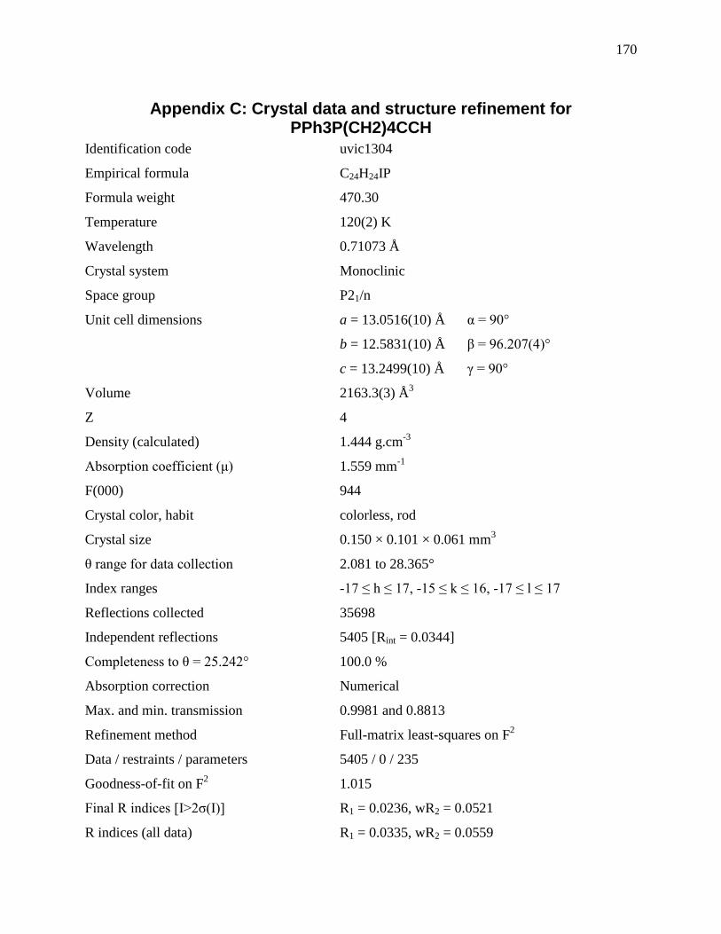
170
Appendix C: Crystal data and structure refinement for PPh3P(CH2)4CCH
Identification code uvic1304
Empirical formula C24H24IP
Formula weight 470.30
Temperature 120(2) K
Wavelength 0.71073 Å
Crystal system Monoclinic
Space group P21/n
Unit cell dimensions a = 13.0516(10) Å α = 90°
b = 12.5831(10) Å β = 96.207(4)°
c = 13.2499(10) Å γ = 90°
Volume 2163.3(3) Å3
Z 4
Density (calculated) 1.444 g.cm-3
Absorption coefficient (μ) 1.559 mm-1
F(000) 944
Crystal color, habit colorless, rod
Crystal size 0.150 × 0.101 × 0.061 mm3
θ range for data collection 2.081 to 28.365°
Index ranges -17 ≤ h ≤ 17, -15 ≤ k ≤ 16, -17 ≤ l ≤ 17
Reflections collected 35698
Independent reflections 5405 [Rint = 0.0344]
Completeness to θ = 25.242° 100.0 %
Absorption correction Numerical
Max. and min. transmission 0.9981 and 0.8813
Refinement method Full-matrix least-squares on F2
Data / restraints / parameters 5405 / 0 / 235
Goodness-of-fit on F2 1.015
Final R indices [I>2σ(I)] R1 = 0.0236, wR2 = 0.0521
R indices (all data) R1 = 0.0335, wR2 = 0.0559

171
Extinction coefficient n/a
Largest diff. peak and hole 0.656 and -0.310 e–.Å
-3
Table 2. Atomic coordinates and equivalent isotropic displacement parameters (Å2)
for uvic1304_x. U(eq) is defined as one third of the trace of the orthogonalized Uij tensor.
x y z U(eq)
P(1) 0.59437(4) 0.35145(4) 0.77633(4) 0.015(1)
C(1) 0.58625(15) 0.34134(15) 0.91035(15) 0.019(1)
C(2) 0.65005(16) 0.24609(16) 0.95519(15) 0.022(1)
C(3) 0.64279(18) 0.23386(18) 1.06805(16) 0.028(1)
C(4) 0.71426(18) 0.14714(18) 1.11623(17) 0.031(1)
C(5) 0.69245(18) 0.0405(2) 1.07102(18) 0.035(1)
C(6) 0.67377(19) -0.0383(2) 1.03465(18) 0.035(1)
C(7) 0.72855(14) 0.35328(14) 0.75839(14) 0.016(1)
C(8) 0.78310(15) 0.44387(16) 0.79383(16) 0.023(1)
C(9) 0.88741(16) 0.45062(17) 0.78475(17) 0.028(1)
C(10) 0.93784(16) 0.36803(18) 0.74190(17) 0.028(1)
C(11) 0.88443(16) 0.27791(17) 0.70810(17) 0.026(1)
C(12) 0.77930(15) 0.27011(15) 0.71609(15) 0.020(1)
C(13) 0.53804(14) 0.47189(14) 0.72400(14) 0.017(1)
C(14) 0.44746(14) 0.51100(15) 0.75743(15) 0.020(1)
C(15) 0.39882(15) 0.59753(16) 0.70789(15) 0.022(1)
C(16) 0.43910(16) 0.64432(16) 0.62686(16) 0.023(1)
C(17) 0.52931(16) 0.60550(16) 0.59386(16) 0.025(1)
C(18) 0.57886(15) 0.51915(16) 0.64136(15) 0.022(1)
C(19) 0.52645(14) 0.24431(14) 0.70879(14) 0.017(1)
C(20) 0.54421(15) 0.22521(15) 0.60839(15) 0.021(1)
C(21) 0.48296(18) 0.15309(16) 0.55023(17) 0.026(1)
C(22) 0.40499(15) 0.09917(16) 0.59120(17) 0.026(1)
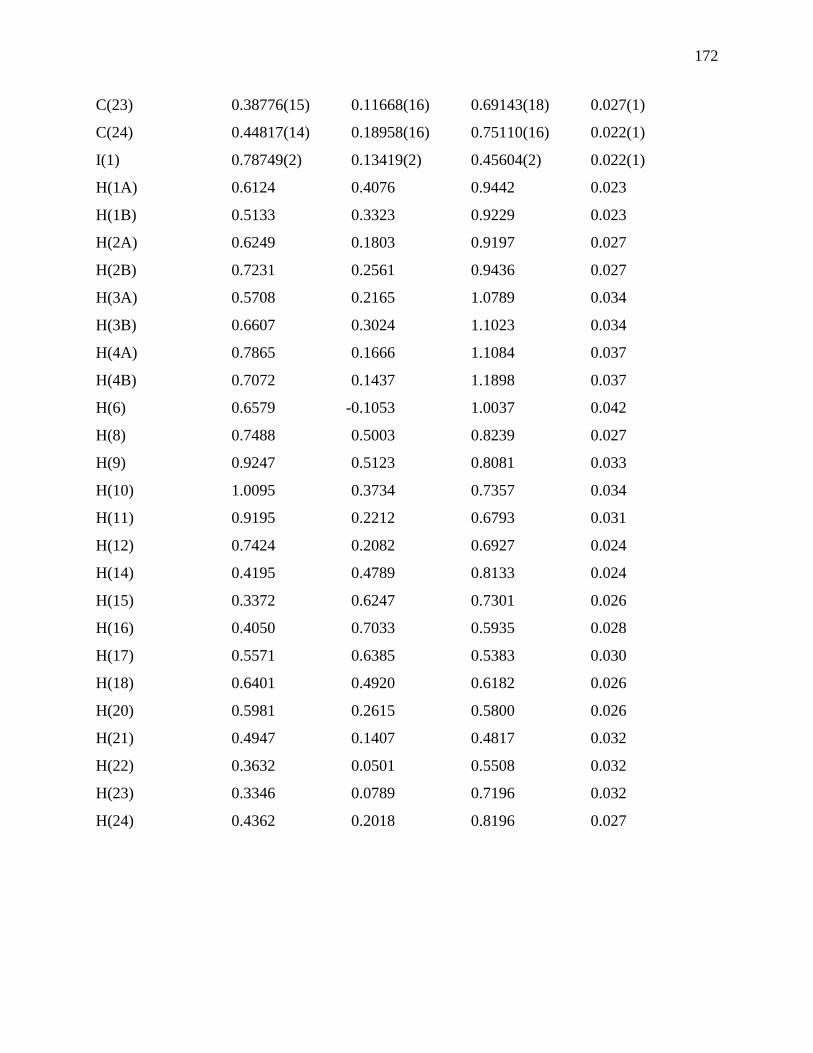
172
C(23) 0.38776(15) 0.11668(16) 0.69143(18) 0.027(1)
C(24) 0.44817(14) 0.18958(16) 0.75110(16) 0.022(1)
I(1) 0.78749(2) 0.13419(2) 0.45604(2) 0.022(1)
H(1A) 0.6124 0.4076 0.9442 0.023
H(1B) 0.5133 0.3323 0.9229 0.023
H(2A) 0.6249 0.1803 0.9197 0.027
H(2B) 0.7231 0.2561 0.9436 0.027
H(3A) 0.5708 0.2165 1.0789 0.034
H(3B) 0.6607 0.3024 1.1023 0.034
H(4A) 0.7865 0.1666 1.1084 0.037
H(4B) 0.7072 0.1437 1.1898 0.037
H(6) 0.6579 -0.1053 1.0037 0.042
H(8) 0.7488 0.5003 0.8239 0.027
H(9) 0.9247 0.5123 0.8081 0.033
H(10) 1.0095 0.3734 0.7357 0.034
H(11) 0.9195 0.2212 0.6793 0.031
H(12) 0.7424 0.2082 0.6927 0.024
H(14) 0.4195 0.4789 0.8133 0.024
H(15) 0.3372 0.6247 0.7301 0.026
H(16) 0.4050 0.7033 0.5935 0.028
H(17) 0.5571 0.6385 0.5383 0.030
H(18) 0.6401 0.4920 0.6182 0.026
H(20) 0.5981 0.2615 0.5800 0.026
H(21) 0.4947 0.1407 0.4817 0.032
H(22) 0.3632 0.0501 0.5508 0.032
H(23) 0.3346 0.0789 0.7196 0.032
H(24) 0.4362 0.2018 0.8196 0.027

173
Table 3. Anisotropic displacement parameters (Å2) for uvic1304_x.
The anisotropic displacement factor exponent takes the form:
-2π2[h
2a*
2U11 + ... + 2hka*b*U12]
U11 U22 U33 U23 U13 U12
P(1) 0.0150(2) 0.0133(2) 0.0165(2) 0.0010(2) 0.0023(2) 0.0000(2)
C(1) 0.0210(9) 0.0210(9) 0.0165(9) 0.0014(7) 0.0043(7) 0.0017(7)
C(2) 0.0242(10) 0.0256(10) 0.0179(10) 0.0034(8) 0.0039(8) 0.0046(8)
C(3) 0.0340(12) 0.0317(11) 0.0191(10) 0.0019(9) 0.0034(9) 0.0039(9)
C(4) 0.0361(12) 0.0358(13) 0.0199(10) 0.0072(9) -0.0042(9) 0.0023(10)
C(5) 0.0318(12) 0.0425(14) 0.0300(12) 0.0176(11) -0.0017(10) 0.0068(11)
C(6) 0.0385(13) 0.0339(13) 0.0309(13) 0.0076(10) -0.0079(10) -0.0082(11)
C(7) 0.0139(8) 0.0172(9) 0.0164(9) 0.0002(7) 0.0011(7) -0.0010(7)
C(8) 0.0226(10) 0.0191(9) 0.0267(11) -0.0056(8) 0.0018(8) -0.0001(8)
C(9) 0.0233(10) 0.0249(10) 0.0342(12) -0.0044(9) 0.0001(9) -0.0084(8)
C(10) 0.0149(9) 0.0399(12) 0.0301(11) -0.0018(10) 0.0037(8) -0.0028(9)
C(11) 0.0217(10) 0.0266(11) 0.0290(11) -0.0045(9) 0.0034(8) 0.0047(8)
C(12) 0.0200(9) 0.0186(9) 0.0217(10) -0.0034(7) 0.0011(8) -0.0001(7)
C(13) 0.0170(9) 0.0135(8) 0.0189(9) -0.0001(7) 0.0006(7) 0.0002(7)
C(14) 0.0195(9) 0.0199(9) 0.0220(10) 0.0020(8) 0.0048(8) -0.0005(8)
C(15) 0.0193(9) 0.0225(9) 0.0243(10) -0.0007(8) 0.0029(8) 0.0036(8)
C(16) 0.0260(10) 0.0191(10) 0.0241(10) 0.0024(8) -0.0013(8) 0.0049(8)
C(17) 0.0302(11) 0.0227(10) 0.0224(10) 0.0054(8) 0.0069(8) 0.0035(8)
C(18) 0.0220(10) 0.0215(10) 0.0225(10) 0.0009(8) 0.0058(8) 0.0031(8)
C(19) 0.0159(9) 0.0137(8) 0.0216(10) 0.0007(7) -0.0012(7) 0.0002(7)
C(20) 0.0247(10) 0.0181(9) 0.0202(10) 0.0029(7) -0.0012(8) -0.0053(8)
C(21) 0.0354(12) 0.0191(10) 0.0230(11) 0.0023(8) -0.0062(9) -0.0023(8)
C(22) 0.0206(10) 0.0175(9) 0.0381(12) -0.0006(9) -0.0085(9) -0.0006(8)
C(23) 0.0146(9) 0.0181(10) 0.0476(14) 0.0015(9) 0.0053(9) -0.0015(7)
C(24) 0.0166(9) 0.0195(10) 0.0321(11) -0.0003(8) 0.0068(8) 0.0016(8)

174
I(1) 0.0215(1) 0.0197(1) 0.0271(1) -0.0048(1) 0.0098(1) -0.0027(1)
Table 4. Bond lengths [Å] for uvic1304_x.
atom-atom distance atom-atom distance
P(1)-C(13) 1.7911(19) P(1)-C(7) 1.7927(19)
P(1)-C(1) 1.795(2) P(1)-C(19) 1.7979(19)
C(1)-C(2) 1.541(3) C(2)-C(3) 1.516(3)
C(3)-C(4) 1.530(3) C(4)-C(5) 1.484(4)
C(5)-C(6) 1.118(3) C(7)-C(12) 1.389(3)
C(7)-C(8) 1.398(3) C(8)-C(9) 1.382(3)
C(9)-C(10) 1.384(3) C(10)-C(11) 1.380(3)
C(11)-C(12) 1.391(3) C(13)-C(14) 1.396(3)
C(13)-C(18) 1.401(3) C(14)-C(15) 1.389(3)
C(15)-C(16) 1.378(3) C(16)-C(17) 1.388(3)
C(17)-C(18) 1.381(3) C(19)-C(20) 1.396(3)
C(19)-C(24) 1.399(3) C(20)-C(21) 1.387(3)
C(21)-C(22) 1.382(3) C(22)-C(23) 1.388(3)
C(23)-C(24) 1.398(3) C(1)-H(1A) 0.9900
C(1)-H(1B) 0.9900 C(2)-H(2A) 0.9900
C(2)-H(2B) 0.9900 C(3)-H(3A) 0.9900
C(3)-H(3B) 0.9900 C(4)-H(4A) 0.9900
C(4)-H(4B) 0.9900 C(6)-H(6) 0.9500
C(8)-H(8) 0.9500 C(9)-H(9) 0.9500
C(10)-H(10) 0.9500 C(11)-H(11) 0.9500
C(12)-H(12) 0.9500 C(14)-H(14) 0.9500
C(15)-H(15) 0.9500 C(16)-H(16) 0.9500
C(17)-H(17) 0.9500 C(18)-H(18) 0.9500
C(20)-H(20) 0.9500 C(21)-H(21) 0.9500
C(22)-H(22) 0.9500 C(23)-H(23) 0.9500

175
C(24)-H(24) 0.9500
Symmetry transformations used to generate equivalent atoms:
Table 5. Bond angles [°] for uvic1304_x.
atom-atom-atom angle atom-atom-atom angle
C(13)-P(1)-C(7) 107.69(9) C(13)-P(1)-C(1) 112.16(9)
C(7)-P(1)-C(1) 107.16(9) C(13)-P(1)-C(19) 106.39(9)
C(7)-P(1)-C(19) 112.32(9) C(1)-P(1)-C(19) 111.14(9)
C(2)-C(1)-P(1) 110.44(13) C(3)-C(2)-C(1) 111.73(17)
C(2)-C(3)-C(4) 112.57(18) C(5)-C(4)-C(3) 113.24(19)
C(6)-C(5)-C(4) 177.7(3) C(12)-C(7)-C(8) 120.15(17)
C(12)-C(7)-P(1) 124.00(14) C(8)-C(7)-P(1) 115.80(14)
C(9)-C(8)-C(7) 119.44(18) C(8)-C(9)-C(10) 120.39(19)
C(11)-C(10)-C(9) 120.27(19) C(10)-C(11)-C(12) 120.07(19)
C(7)-C(12)-C(11) 119.67(18) C(14)-C(13)-C(18) 120.33(17)
C(14)-C(13)-P(1) 120.11(14) C(18)-C(13)-P(1) 119.13(14)
C(15)-C(14)-C(13) 119.06(18) C(16)-C(15)-C(14) 120.66(18)
C(15)-C(16)-C(17) 120.21(18) C(18)-C(17)-C(16) 120.31(19)
C(17)-C(18)-C(13) 119.42(18) C(20)-C(19)-C(24) 120.07(17)
C(20)-C(19)-P(1) 118.67(14) C(24)-C(19)-P(1) 120.80(15)
C(21)-C(20)-C(19) 119.81(19) C(22)-C(21)-C(20) 120.5(2)
C(21)-C(22)-C(23) 120.01(19) C(22)-C(23)-C(24) 120.36(19)
C(23)-C(24)-C(19) 119.23(19) C(2)-C(1)-H(1A) 109.6
P(1)-C(1)-H(1A) 109.6 C(2)-C(1)-H(1B) 109.6
P(1)-C(1)-H(1B) 109.6 H(1A)-C(1)-H(1B) 108.1
C(3)-C(2)-H(2A) 109.3 C(1)-C(2)-H(2A) 109.3
C(3)-C(2)-H(2B) 109.3 C(1)-C(2)-H(2B) 109.3
H(2A)-C(2)-H(2B) 107.9 C(2)-C(3)-H(3A) 109.1
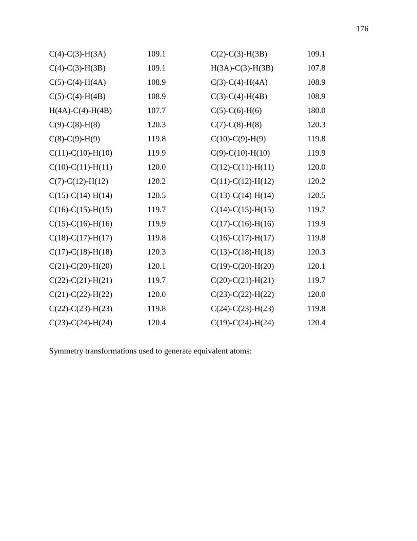
176
C(4)-C(3)-H(3A) 109.1 C(2)-C(3)-H(3B) 109.1
C(4)-C(3)-H(3B) 109.1 H(3A)-C(3)-H(3B) 107.8
C(5)-C(4)-H(4A) 108.9 C(3)-C(4)-H(4A) 108.9
C(5)-C(4)-H(4B) 108.9 C(3)-C(4)-H(4B) 108.9
H(4A)-C(4)-H(4B) 107.7 C(5)-C(6)-H(6) 180.0
C(9)-C(8)-H(8) 120.3 C(7)-C(8)-H(8) 120.3
C(8)-C(9)-H(9) 119.8 C(10)-C(9)-H(9) 119.8
C(11)-C(10)-H(10) 119.9 C(9)-C(10)-H(10) 119.9
C(10)-C(11)-H(11) 120.0 C(12)-C(11)-H(11) 120.0
C(7)-C(12)-H(12) 120.2 C(11)-C(12)-H(12) 120.2
C(15)-C(14)-H(14) 120.5 C(13)-C(14)-H(14) 120.5
C(16)-C(15)-H(15) 119.7 C(14)-C(15)-H(15) 119.7
C(15)-C(16)-H(16) 119.9 C(17)-C(16)-H(16) 119.9
C(18)-C(17)-H(17) 119.8 C(16)-C(17)-H(17) 119.8
C(17)-C(18)-H(18) 120.3 C(13)-C(18)-H(18) 120.3
C(21)-C(20)-H(20) 120.1 C(19)-C(20)-H(20) 120.1
C(22)-C(21)-H(21) 119.7 C(20)-C(21)-H(21) 119.7
C(21)-C(22)-H(22) 120.0 C(23)-C(22)-H(22) 120.0
C(22)-C(23)-H(23) 119.8 C(24)-C(23)-H(23) 119.8
C(23)-C(24)-H(24) 120.4 C(19)-C(24)-H(24) 120.4
Symmetry transformations used to generate equivalent atoms:
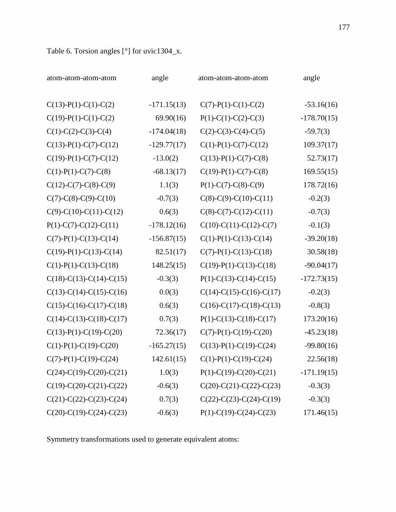
177
Table 6. Torsion angles [°] for uvic1304_x.
atom-atom-atom-atom angle atom-atom-atom-atom angle
C(13)-P(1)-C(1)-C(2) -171.15(13) C(7)-P(1)-C(1)-C(2) -53.16(16)
C(19)-P(1)-C(1)-C(2) 69.90(16) P(1)-C(1)-C(2)-C(3) -178.70(15)
C(1)-C(2)-C(3)-C(4) -174.04(18) C(2)-C(3)-C(4)-C(5) -59.7(3)
C(13)-P(1)-C(7)-C(12) -129.77(17) C(1)-P(1)-C(7)-C(12) 109.37(17)
C(19)-P(1)-C(7)-C(12) -13.0(2) C(13)-P(1)-C(7)-C(8) 52.73(17)
C(1)-P(1)-C(7)-C(8) -68.13(17) C(19)-P(1)-C(7)-C(8) 169.55(15)
C(12)-C(7)-C(8)-C(9) 1.1(3) P(1)-C(7)-C(8)-C(9) 178.72(16)
C(7)-C(8)-C(9)-C(10) -0.7(3) C(8)-C(9)-C(10)-C(11) -0.2(3)
C(9)-C(10)-C(11)-C(12) 0.6(3) C(8)-C(7)-C(12)-C(11) -0.7(3)
P(1)-C(7)-C(12)-C(11) -178.12(16) C(10)-C(11)-C(12)-C(7) -0.1(3)
C(7)-P(1)-C(13)-C(14) -156.87(15) C(1)-P(1)-C(13)-C(14) -39.20(18)
C(19)-P(1)-C(13)-C(14) 82.51(17) C(7)-P(1)-C(13)-C(18) 30.58(18)
C(1)-P(1)-C(13)-C(18) 148.25(15) C(19)-P(1)-C(13)-C(18) -90.04(17)
C(18)-C(13)-C(14)-C(15) -0.3(3) P(1)-C(13)-C(14)-C(15) -172.73(15)
C(13)-C(14)-C(15)-C(16) 0.0(3) C(14)-C(15)-C(16)-C(17) -0.2(3)
C(15)-C(16)-C(17)-C(18) 0.6(3) C(16)-C(17)-C(18)-C(13) -0.8(3)
C(14)-C(13)-C(18)-C(17) 0.7(3) P(1)-C(13)-C(18)-C(17) 173.20(16)
C(13)-P(1)-C(19)-C(20) 72.36(17) C(7)-P(1)-C(19)-C(20) -45.23(18)
C(1)-P(1)-C(19)-C(20) -165.27(15) C(13)-P(1)-C(19)-C(24) -99.80(16)
C(7)-P(1)-C(19)-C(24) 142.61(15) C(1)-P(1)-C(19)-C(24) 22.56(18)
C(24)-C(19)-C(20)-C(21) 1.0(3) P(1)-C(19)-C(20)-C(21) -171.19(15)
C(19)-C(20)-C(21)-C(22) -0.6(3) C(20)-C(21)-C(22)-C(23) -0.3(3)
C(21)-C(22)-C(23)-C(24) 0.7(3) C(22)-C(23)-C(24)-C(19) -0.3(3)
C(20)-C(19)-C(24)-C(23) -0.6(3) P(1)-C(19)-C(24)-C(23) 171.46(15)
Symmetry transformations used to generate equivalent atoms:
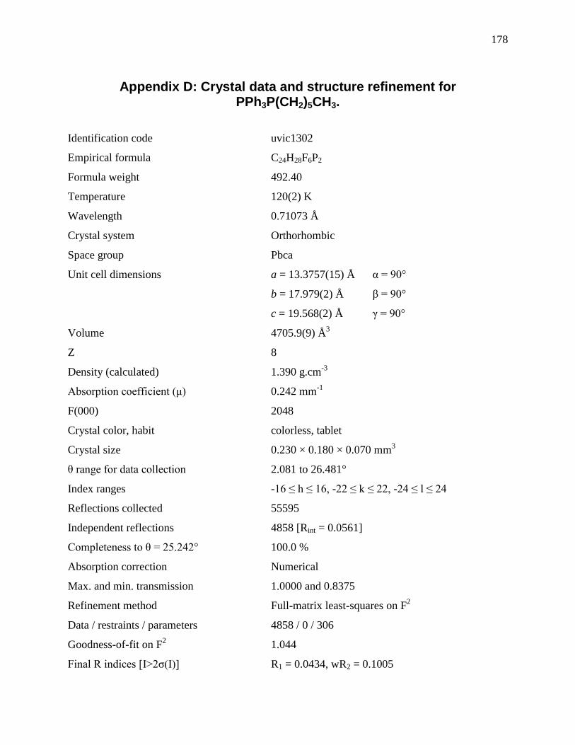
178
Appendix D: Crystal data and structure refinement for PPh3P(CH2)5CH3.
Identification code uvic1302
Empirical formula C24H28F6P2
Formula weight 492.40
Temperature 120(2) K
Wavelength 0.71073 Å
Crystal system Orthorhombic
Space group Pbca
Unit cell dimensions a = 13.3757(15) Å α = 90°
b = 17.979(2) Å β = 90°
c = 19.568(2) Å γ = 90°
Volume 4705.9(9) Å3
Z 8
Density (calculated) 1.390 g.cm-3
Absorption coefficient (μ) 0.242 mm-1
F(000) 2048
Crystal color, habit colorless, tablet
Crystal size 0.230 × 0.180 × 0.070 mm3
θ range for data collection 2.081 to 26.481°
Index ranges -16 ≤ h ≤ 16, -22 ≤ k ≤ 22, -24 ≤ l ≤ 24
Reflections collected 55595
Independent reflections 4858 [Rint = 0.0561]
Completeness to θ = 25.242° 100.0 %
Absorption correction Numerical
Max. and min. transmission 1.0000 and 0.8375
Refinement method Full-matrix least-squares on F2
Data / restraints / parameters 4858 / 0 / 306
Goodness-of-fit on F2 1.044
Final R indices [I>2σ(I)] R1 = 0.0434, wR2 = 0.1005
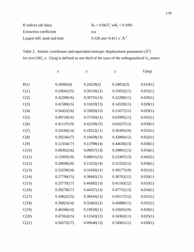
179
R indices (all data) R1 = 0.0637, wR2 = 0.1091
Extinction coefficient n/a
Largest diff. peak and hole 0.528 and -0.451 e–.Å
-3
Table 2. Atomic coordinates and equivalent isotropic displacement parameters (Å2)
for uvic1302_x. U(eq) is defined as one third of the trace of the orthogonalized Uij tensor.
x y z U(eq)
P(1) 0.34382(4) 0.24259(3) 0.34052(3) 0.019(1)
C(1) 0.33641(15) 0.26159(12) 0.25052(11) 0.025(1)
C(2) 0.42290(16) 0.30731(13) 0.22289(11) 0.029(1)
C(3) 0.41580(15) 0.31619(13) 0.14559(11) 0.028(1)
C(4) 0.50425(16) 0.35820(13) 0.11677(11) 0.029(1)
C(5) 0.49729(16) 0.37350(12) 0.03995(11) 0.031(1)
C(6) 0.41137(19) 0.42259(15) 0.02027(12) 0.039(1)
C(7) 0.24166(14) 0.18222(11) 0.36305(10) 0.023(1)
C(8) 0.20236(17) 0.18428(13) 0.42860(12) 0.032(1)
C(9) 0.12354(17) 0.13798(14) 0.44630(13) 0.038(1)
C(10) 0.08302(16) 0.09057(13) 0.39891(13) 0.034(1)
C(11) 0.12095(19) 0.08831(15) 0.33387(13) 0.042(1)
C(12) 0.20049(18) 0.13332(14) 0.31552(12) 0.036(1)
C(13) 0.33259(14) 0.32456(11) 0.39177(10) 0.021(1)
C(14) 0.27700(15) 0.38445(12) 0.36762(11) 0.026(1)
C(15) 0.25770(17) 0.44382(13) 0.41103(12) 0.033(1)
C(16) 0.29278(17) 0.44357(13) 0.47731(13) 0.034(1)
C(17) 0.34822(15) 0.38416(13) 0.50117(12) 0.031(1)
C(18) 0.36825(14) 0.32465(12) 0.45880(11) 0.025(1)
C(19) 0.46246(14) 0.19939(11) 0.35605(10) 0.020(1)
C(20) 0.47263(15) 0.12343(12) 0.34363(11) 0.025(1)
C(21) 0.56572(17) 0.09040(13) 0.34961(11) 0.030(1)
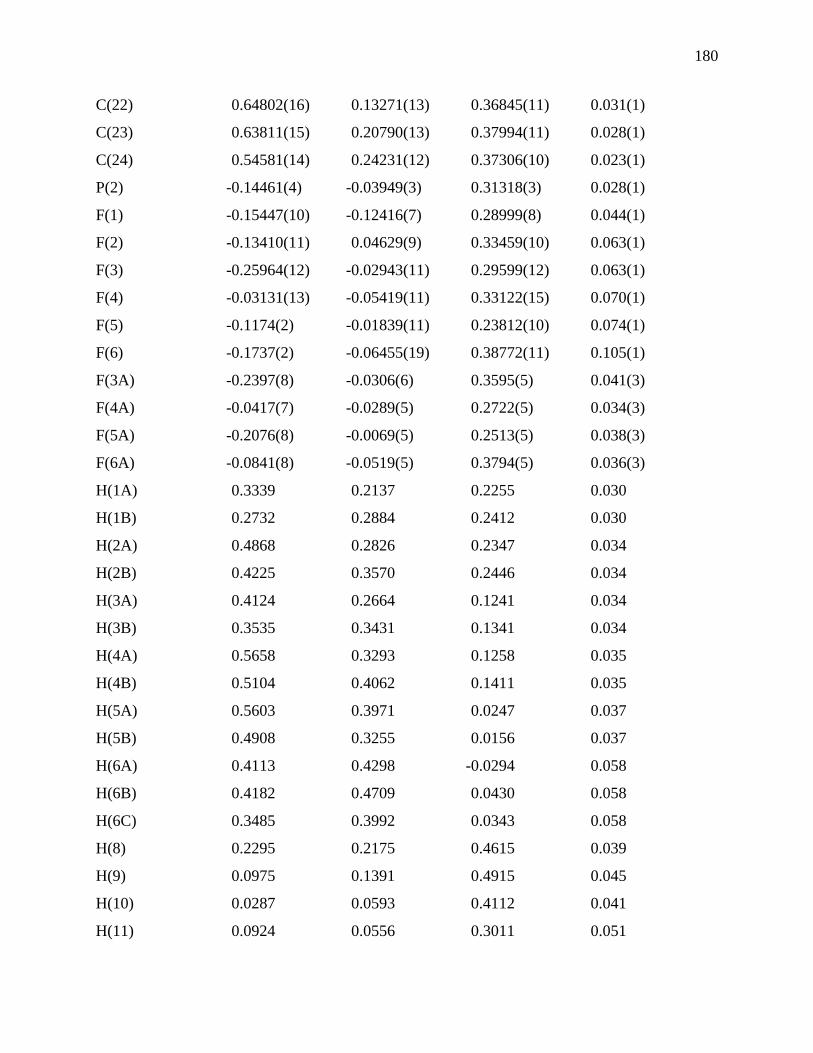
180
C(22) 0.64802(16) 0.13271(13) 0.36845(11) 0.031(1)
C(23) 0.63811(15) 0.20790(13) 0.37994(11) 0.028(1)
C(24) 0.54581(14) 0.24231(12) 0.37306(10) 0.023(1)
P(2) -0.14461(4) -0.03949(3) 0.31318(3) 0.028(1)
F(1) -0.15447(10) -0.12416(7) 0.28999(8) 0.044(1)
F(2) -0.13410(11) 0.04629(9) 0.33459(10) 0.063(1)
F(3) -0.25964(12) -0.02943(11) 0.29599(12) 0.063(1)
F(4) -0.03131(13) -0.05419(11) 0.33122(15) 0.070(1)
F(5) -0.1174(2) -0.01839(11) 0.23812(10) 0.074(1)
F(6) -0.1737(2) -0.06455(19) 0.38772(11) 0.105(1)
F(3A) -0.2397(8) -0.0306(6) 0.3595(5) 0.041(3)
F(4A) -0.0417(7) -0.0289(5) 0.2722(5) 0.034(3)
F(5A) -0.2076(8) -0.0069(5) 0.2513(5) 0.038(3)
F(6A) -0.0841(8) -0.0519(5) 0.3794(5) 0.036(3)
H(1A) 0.3339 0.2137 0.2255 0.030
H(1B) 0.2732 0.2884 0.2412 0.030
H(2A) 0.4868 0.2826 0.2347 0.034
H(2B) 0.4225 0.3570 0.2446 0.034
H(3A) 0.4124 0.2664 0.1241 0.034
H(3B) 0.3535 0.3431 0.1341 0.034
H(4A) 0.5658 0.3293 0.1258 0.035
H(4B) 0.5104 0.4062 0.1411 0.035
H(5A) 0.5603 0.3971 0.0247 0.037
H(5B) 0.4908 0.3255 0.0156 0.037
H(6A) 0.4113 0.4298 -0.0294 0.058
H(6B) 0.4182 0.4709 0.0430 0.058
H(6C) 0.3485 0.3992 0.0343 0.058
H(8) 0.2295 0.2175 0.4615 0.039
H(9) 0.0975 0.1391 0.4915 0.045
H(10) 0.0287 0.0593 0.4112 0.041
H(11) 0.0924 0.0556 0.3011 0.051
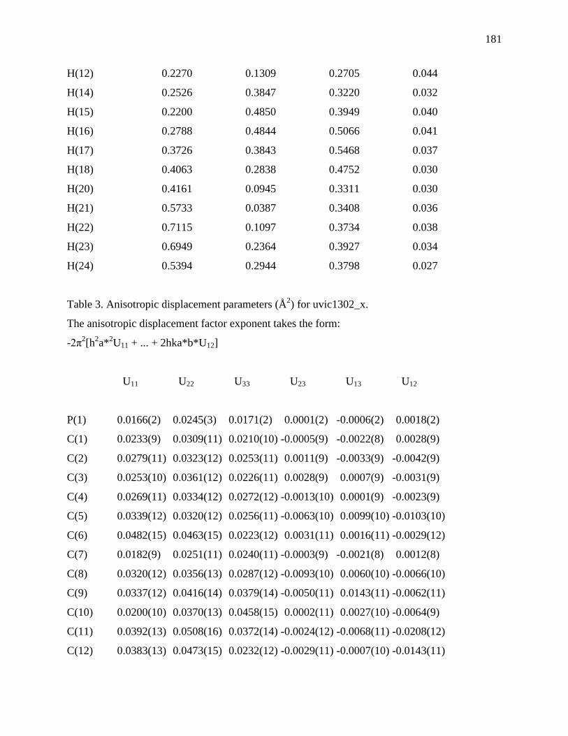
181
H(12) 0.2270 0.1309 0.2705 0.044
H(14) 0.2526 0.3847 0.3220 0.032
H(15) 0.2200 0.4850 0.3949 0.040
H(16) 0.2788 0.4844 0.5066 0.041
H(17) 0.3726 0.3843 0.5468 0.037
H(18) 0.4063 0.2838 0.4752 0.030
H(20) 0.4161 0.0945 0.3311 0.030
H(21) 0.5733 0.0387 0.3408 0.036
H(22) 0.7115 0.1097 0.3734 0.038
H(23) 0.6949 0.2364 0.3927 0.034
H(24) 0.5394 0.2944 0.3798 0.027
Table 3. Anisotropic displacement parameters (Å2) for uvic1302_x.
The anisotropic displacement factor exponent takes the form:
-2π2[h
2a*
2U11 + ... + 2hka*b*U12]
U11 U22 U33 U23 U13 U12
P(1) 0.0166(2) 0.0245(3) 0.0171(2) 0.0001(2) -0.0006(2) 0.0018(2)
C(1) 0.0233(9) 0.0309(11) 0.0210(10) -0.0005(9) -0.0022(8) 0.0028(9)
C(2) 0.0279(11) 0.0323(12) 0.0253(11) 0.0011(9) -0.0033(9) -0.0042(9)
C(3) 0.0253(10) 0.0361(12) 0.0226(11) 0.0028(9) 0.0007(9) -0.0031(9)
C(4) 0.0269(11) 0.0334(12) 0.0272(12) -0.0013(10) 0.0001(9) -0.0023(9)
C(5) 0.0339(12) 0.0320(12) 0.0256(11) -0.0063(10) 0.0099(10) -0.0103(10)
C(6) 0.0482(15) 0.0463(15) 0.0223(12) 0.0031(11) 0.0016(11) -0.0029(12)
C(7) 0.0182(9) 0.0251(11) 0.0240(11) -0.0003(9) -0.0021(8) 0.0012(8)
C(8) 0.0320(12) 0.0356(13) 0.0287(12) -0.0093(10) 0.0060(10) -0.0066(10)
C(9) 0.0337(12) 0.0416(14) 0.0379(14) -0.0050(11) 0.0143(11) -0.0062(11)
C(10) 0.0200(10) 0.0370(13) 0.0458(15) 0.0002(11) 0.0027(10) -0.0064(9)
C(11) 0.0392(13) 0.0508(16) 0.0372(14) -0.0024(12) -0.0068(11) -0.0208(12)
C(12) 0.0383(13) 0.0473(15) 0.0232(12) -0.0029(11) -0.0007(10) -0.0143(11)
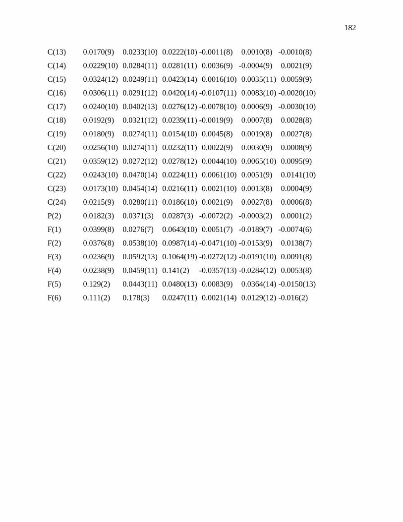
182
C(13) 0.0170(9) 0.0233(10) 0.0222(10) -0.0011(8) 0.0010(8) -0.0010(8)
C(14) 0.0229(10) 0.0284(11) 0.0281(11) 0.0036(9) -0.0004(9) 0.0021(9)
C(15) 0.0324(12) 0.0249(11) 0.0423(14) 0.0016(10) 0.0035(11) 0.0059(9)
C(16) 0.0306(11) 0.0291(12) 0.0420(14) -0.0107(11) 0.0083(10) -0.0020(10)
C(17) 0.0240(10) 0.0402(13) 0.0276(12) -0.0078(10) 0.0006(9) -0.0030(10)
C(18) 0.0192(9) 0.0321(12) 0.0239(11) -0.0019(9) 0.0007(8) 0.0028(8)
C(19) 0.0180(9) 0.0274(11) 0.0154(10) 0.0045(8) 0.0019(8) 0.0027(8)
C(20) 0.0256(10) 0.0274(11) 0.0232(11) 0.0022(9) 0.0030(9) 0.0008(9)
C(21) 0.0359(12) 0.0272(12) 0.0278(12) 0.0044(10) 0.0065(10) 0.0095(9)
C(22) 0.0243(10) 0.0470(14) 0.0224(11) 0.0061(10) 0.0051(9) 0.0141(10)
C(23) 0.0173(10) 0.0454(14) 0.0216(11) 0.0021(10) 0.0013(8) 0.0004(9)
C(24) 0.0215(9) 0.0280(11) 0.0186(10) 0.0021(9) 0.0027(8) 0.0006(8)
P(2) 0.0182(3) 0.0371(3) 0.0287(3) -0.0072(2) -0.0003(2) 0.0001(2)
F(1) 0.0399(8) 0.0276(7) 0.0643(10) 0.0051(7) -0.0189(7) -0.0074(6)
F(2) 0.0376(8) 0.0538(10) 0.0987(14) -0.0471(10) -0.0153(9) 0.0138(7)
F(3) 0.0236(9) 0.0592(13) 0.1064(19) -0.0272(12) -0.0191(10) 0.0091(8)
F(4) 0.0238(9) 0.0459(11) 0.141(2) -0.0357(13) -0.0284(12) 0.0053(8)
F(5) 0.129(2) 0.0443(11) 0.0480(13) 0.0083(9) 0.0364(14) -0.0150(13)
F(6) 0.111(2) 0.178(3) 0.0247(11) 0.0021(14) 0.0129(12) -0.016(2)

183
Table 4. Bond lengths [Å] for uvic1302_x.
atom-atom distance atom-atom distance
P(1)-C(13) 1.789(2) P(1)-C(19) 1.793(2)
P(1)-C(1) 1.797(2) P(1)-C(7) 1.800(2)
C(1)-C(2) 1.519(3) C(2)-C(3) 1.524(3)
C(3)-C(4) 1.513(3) C(4)-C(5) 1.531(3)
C(5)-C(6) 1.499(3) C(7)-C(8) 1.387(3)
C(7)-C(12) 1.393(3) C(8)-C(9) 1.387(3)
C(9)-C(10) 1.371(3) C(10)-C(11) 1.371(3)
C(11)-C(12) 1.384(3) C(13)-C(14) 1.391(3)
C(13)-C(18) 1.396(3) C(14)-C(15) 1.388(3)
C(15)-C(16) 1.379(3) C(16)-C(17) 1.382(3)
C(17)-C(18) 1.380(3) C(19)-C(20) 1.394(3)
C(19)-C(24) 1.396(3) C(20)-C(21) 1.385(3)
C(21)-C(22) 1.388(3) C(22)-C(23) 1.377(3)
C(23)-C(24) 1.388(3) P(2)-F(6A) 1.545(9)
P(2)-F(5) 1.560(2) P(2)-F(3A) 1.569(10)
P(2)-F(6) 1.575(2) P(2)-F(4) 1.5783(17)
P(2)-F(3) 1.5853(17) P(2)-F(5A) 1.588(9)
P(2)-F(1) 1.5939(15) P(2)-F(2) 1.6043(16)
P(2)-F(4A) 1.605(9) C(1)-H(1A) 0.9900
C(1)-H(1B) 0.9900 C(2)-H(2A) 0.9900
C(2)-H(2B) 0.9900 C(3)-H(3A) 0.9900
C(3)-H(3B) 0.9900 C(4)-H(4A) 0.9900
C(4)-H(4B) 0.9900 C(5)-H(5A) 0.9900
C(5)-H(5B) 0.9900 C(6)-H(6A) 0.9800
C(6)-H(6B) 0.9800 C(6)-H(6C) 0.9800
C(8)-H(8) 0.9500 C(9)-H(9) 0.9500
C(10)-H(10) 0.9500 C(11)-H(11) 0.9500
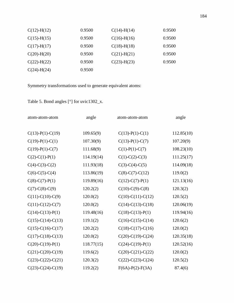
184
C(12)-H(12) 0.9500 C(14)-H(14) 0.9500
C(15)-H(15) 0.9500 C(16)-H(16) 0.9500
C(17)-H(17) 0.9500 C(18)-H(18) 0.9500
C(20)-H(20) 0.9500 C(21)-H(21) 0.9500
C(22)-H(22) 0.9500 C(23)-H(23) 0.9500
C(24)-H(24) 0.9500
Symmetry transformations used to generate equivalent atoms:
Table 5. Bond angles [°] for uvic1302_x.
atom-atom-atom angle atom-atom-atom angle
C(13)-P(1)-C(19) 109.65(9) C(13)-P(1)-C(1) 112.85(10)
C(19)-P(1)-C(1) 107.30(9) C(13)-P(1)-C(7) 107.20(9)
C(19)-P(1)-C(7) 111.68(9) C(1)-P(1)-C(7) 108.23(10)
C(2)-C(1)-P(1) 114.19(14) C(1)-C(2)-C(3) 111.25(17)
C(4)-C(3)-C(2) 111.93(18) C(3)-C(4)-C(5) 114.09(18)
C(6)-C(5)-C(4) 113.86(19) C(8)-C(7)-C(12) 119.0(2)
C(8)-C(7)-P(1) 119.89(16) C(12)-C(7)-P(1) 121.13(16)
C(7)-C(8)-C(9) 120.2(2) C(10)-C(9)-C(8) 120.3(2)
C(11)-C(10)-C(9) 120.0(2) C(10)-C(11)-C(12) 120.5(2)
C(11)-C(12)-C(7) 120.0(2) C(14)-C(13)-C(18) 120.06(19)
C(14)-C(13)-P(1) 119.48(16) C(18)-C(13)-P(1) 119.94(16)
C(15)-C(14)-C(13) 119.1(2) C(16)-C(15)-C(14) 120.6(2)
C(15)-C(16)-C(17) 120.2(2) C(18)-C(17)-C(16) 120.0(2)
C(17)-C(18)-C(13) 120.0(2) C(20)-C(19)-C(24) 120.35(18)
C(20)-C(19)-P(1) 118.77(15) C(24)-C(19)-P(1) 120.52(16)
C(21)-C(20)-C(19) 119.6(2) C(20)-C(21)-C(22) 120.0(2)
C(23)-C(22)-C(21) 120.3(2) C(22)-C(23)-C(24) 120.5(2)
C(23)-C(24)-C(19) 119.2(2) F(6A)-P(2)-F(3A) 87.4(6)

185
F(5)-P(2)-F(6) 177.28(14) F(5)-P(2)-F(4) 91.56(15)
F(6)-P(2)-F(4) 88.99(16) F(5)-P(2)-F(3) 89.94(14)
F(6)-P(2)-F(3) 89.39(15) F(4)-P(2)-F(3) 176.83(12)
F(6A)-P(2)-F(5A) 166.3(5) F(3A)-P(2)-F(5A) 88.5(6)
F(6A)-P(2)-F(1) 98.3(4) F(5)-P(2)-F(1) 89.05(10)
F(3A)-P(2)-F(1) 101.2(4) F(6)-P(2)-F(1) 88.28(14)
F(4)-P(2)-F(1) 89.04(8) F(3)-P(2)-F(1) 88.18(9)
F(5A)-P(2)-F(1) 95.2(3) F(6A)-P(2)-F(2) 82.7(4)
F(5)-P(2)-F(2) 89.51(11) F(3A)-P(2)-F(2) 79.8(4)
F(6)-P(2)-F(2) 93.14(14) F(4)-P(2)-F(2) 91.05(9)
F(3)-P(2)-F(2) 91.76(9) F(5A)-P(2)-F(2) 83.7(3)
F(1)-P(2)-F(2) 178.57(10) F(6A)-P(2)-F(4A) 89.2(5)
F(3A)-P(2)-F(4A) 166.3(5) F(5A)-P(2)-F(4A) 91.7(6)
F(1)-P(2)-F(4A) 92.4(3) F(2)-P(2)-F(4A) 86.6(3)
C(2)-C(1)-H(1A) 108.7 P(1)-C(1)-H(1A) 108.7
C(2)-C(1)-H(1B) 108.7 P(1)-C(1)-H(1B) 108.7
H(1A)-C(1)-H(1B) 107.6 C(1)-C(2)-H(2A) 109.4
C(3)-C(2)-H(2A) 109.4 C(1)-C(2)-H(2B) 109.4
C(3)-C(2)-H(2B) 109.4 H(2A)-C(2)-H(2B) 108.0
C(4)-C(3)-H(3A) 109.2 C(2)-C(3)-H(3A) 109.2
C(4)-C(3)-H(3B) 109.2 C(2)-C(3)-H(3B) 109.2
H(3A)-C(3)-H(3B) 107.9 C(3)-C(4)-H(4A) 108.7
C(5)-C(4)-H(4A) 108.7 C(3)-C(4)-H(4B) 108.7
C(5)-C(4)-H(4B) 108.7 H(4A)-C(4)-H(4B) 107.6
C(6)-C(5)-H(5A) 108.8 C(4)-C(5)-H(5A) 108.8
C(6)-C(5)-H(5B) 108.8 C(4)-C(5)-H(5B) 108.8
H(5A)-C(5)-H(5B) 107.7 C(5)-C(6)-H(6A) 109.5
C(5)-C(6)-H(6B) 109.5 H(6A)-C(6)-H(6B) 109.5
C(5)-C(6)-H(6C) 109.5 H(6A)-C(6)-H(6C) 109.5
H(6B)-C(6)-H(6C) 109.5 C(7)-C(8)-H(8) 119.9
C(9)-C(8)-H(8) 119.9 C(10)-C(9)-H(9) 119.8
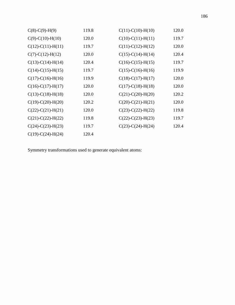
186
C(8)-C(9)-H(9) 119.8 C(11)-C(10)-H(10) 120.0
C(9)-C(10)-H(10) 120.0 C(10)-C(11)-H(11) 119.7
C(12)-C(11)-H(11) 119.7 C(11)-C(12)-H(12) 120.0
C(7)-C(12)-H(12) 120.0 C(15)-C(14)-H(14) 120.4
C(13)-C(14)-H(14) 120.4 C(16)-C(15)-H(15) 119.7
C(14)-C(15)-H(15) 119.7 C(15)-C(16)-H(16) 119.9
C(17)-C(16)-H(16) 119.9 C(18)-C(17)-H(17) 120.0
C(16)-C(17)-H(17) 120.0 C(17)-C(18)-H(18) 120.0
C(13)-C(18)-H(18) 120.0 C(21)-C(20)-H(20) 120.2
C(19)-C(20)-H(20) 120.2 C(20)-C(21)-H(21) 120.0
C(22)-C(21)-H(21) 120.0 C(23)-C(22)-H(22) 119.8
C(21)-C(22)-H(22) 119.8 C(22)-C(23)-H(23) 119.7
C(24)-C(23)-H(23) 119.7 C(23)-C(24)-H(24) 120.4
C(19)-C(24)-H(24) 120.4
Symmetry transformations used to generate equivalent atoms:

187
Table 6. Torsion angles [°] for uvic1302_x.
atom-atom-atom-atom angle atom-atom-atom-atom angle
C(13)-P(1)-C(1)-C(2) 66.03(18) C(19)-P(1)-C(1)-C(2) -54.85(18)
C(7)-P(1)-C(1)-C(2) -175.51(15) P(1)-C(1)-C(2)-C(3) 175.67(15)
C(1)-C(2)-C(3)-C(4) -177.04(18) C(2)-C(3)-C(4)-C(5) -175.91(19)
C(3)-C(4)-C(5)-C(6) 63.3(3) C(13)-P(1)-C(7)-C(8) -29.7(2)
C(19)-P(1)-C(7)-C(8) 90.44(19) C(1)-P(1)-C(7)-C(8) -151.67(17)
C(13)-P(1)-C(7)-C(12) 149.98(18) C(19)-P(1)-C(7)-C(12) -89.9(2)
C(1)-P(1)-C(7)-C(12) 28.0(2) C(12)-C(7)-C(8)-C(9) 0.2(3)
P(1)-C(7)-C(8)-C(9) 179.92(19) C(7)-C(8)-C(9)-C(10) -0.9(4)
C(8)-C(9)-C(10)-C(11) 0.6(4) C(9)-C(10)-C(11)-C(12) 0.3(4)
C(10)-C(11)-C(12)-C(7) -1.0(4) C(8)-C(7)-C(12)-C(11) 0.6(4)
P(1)-C(7)-C(12)-C(11) -179.0(2) C(19)-P(1)-C(13)-C(14) 148.69(16)
C(1)-P(1)-C(13)-C(14) 29.16(19) C(7)-P(1)-C(13)-C(14) -89.91(18)
C(19)-P(1)-C(13)-C(18) -39.57(18) C(1)-P(1)-C(13)-C(18) -159.10(15)
C(7)-P(1)-C(13)-C(18) 81.83(17) C(18)-C(13)-C(14)-C(15) 0.0(3)
P(1)-C(13)-C(14)-C(15) 171.68(16) C(13)-C(14)-C(15)-C(16) -0.2(3)
C(14)-C(15)-C(16)-C(17) 0.4(3) C(15)-C(16)-C(17)-C(18) -0.3(3)
C(16)-C(17)-C(18)-C(13) 0.1(3) C(14)-C(13)-C(18)-C(17) 0.1(3)
P(1)-C(13)-C(18)-C(17) -171.60(16) C(13)-P(1)-C(19)-C(20) 155.52(16)
C(1)-P(1)-C(19)-C(20) -81.60(17) C(7)-P(1)-C(19)-C(20) 36.85(19)
C(13)-P(1)-C(19)-C(24) -31.37(19) C(1)-P(1)-C(19)-C(24) 91.51(17)
C(7)-P(1)-C(19)-C(24) -150.04(16) C(24)-C(19)-C(20)-C(21) 1.3(3)
P(1)-C(19)-C(20)-C(21) 174.41(16) C(19)-C(20)-C(21)-C(22) 0.6(3)
C(20)-C(21)-C(22)-C(23) -1.3(3) C(21)-C(22)-C(23)-C(24) 0.2(3)
C(22)-C(23)-C(24)-C(19) 1.7(3) C(20)-C(19)-C(24)-C(23) -2.4(3)
P(1)-C(19)-C(24)-C(23) -175.39(15)
Symmetry transformations used to generate equivalent atoms:
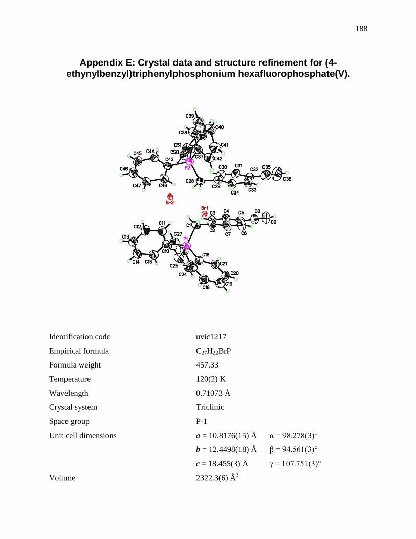
188
Appendix E: Crystal data and structure refinement for (4-ethynylbenzyl)triphenylphosphonium hexafluorophosphate(V).
Identification code uvic1217
Empirical formula C27H22BrP
Formula weight 457.33
Temperature 120(2) K
Wavelength 0.71073 Å
Crystal system Triclinic
Space group P-1
Unit cell dimensions a = 10.8176(15) Å α = 98.278(3)°
b = 12.4498(18) Å β = 94.561(3)°
c = 18.455(3) Å γ = 107.751(3)°
Volume 2322.3(6) Å3
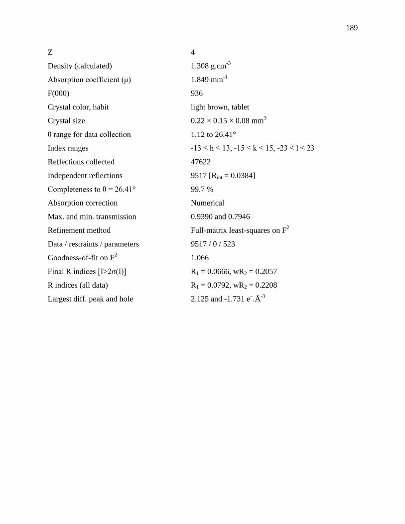
189
Z 4
Density (calculated) 1.308 g.cm-3
Absorption coefficient (μ) 1.849 mm-1
F(000) 936
Crystal color, habit light brown, tablet
Crystal size 0.22 × 0.15 × 0.08 mm3
θ range for data collection 1.12 to 26.41°
Index ranges -13 ≤ h ≤ 13, -15 ≤ k ≤ 15, -23 ≤ l ≤ 23
Reflections collected 47622
Independent reflections 9517 [Rint = 0.0384]
Completeness to θ = 26.41° 99.7 %
Absorption correction Numerical
Max. and min. transmission 0.9390 and 0.7946
Refinement method Full-matrix least-squares on F2
Data / restraints / parameters 9517 / 0 / 523
Goodness-of-fit on F2 1.066
Final R indices [I>2σ(I)] R1 = 0.0666, wR2 = 0.2057
R indices (all data) R1 = 0.0792, wR2 = 0.2208
Largest diff. peak and hole 2.125 and -1.731 e–.Å
-3

190
Table 2. Atomic coordinates and equivalent isotropic displacement parameters (Å2)
for uvic1217. U(eq) is defined as one third of the trace of the orthogonalized Uij tensor.
x y z U(eq)
Br(1) 0.77064(4) -0.00819(4) 0.13317(2) 0.016(1)
Br(2) 0.54519(5) 0.42038(4) 0.26878(3) 0.027(1)
P(1) 0.88338(17) 0.39375(14) 0.12470(10) 0.039(1)
C(1) 0.8298(7) 0.3242(6) 0.2018(4) 0.046(2)
C(2) 0.9266(7) 0.3632(6) 0.2713(4) 0.044(2)
C(3) 0.9253(7) 0.4538(6) 0.3238(4) 0.045(2)
C(4) 1.0120(7) 0.4873(6) 0.3887(4) 0.047(2)
C(5) 1.1034(8) 0.4337(6) 0.4019(4) 0.049(2)
C(6) 1.1048(10) 0.3411(8) 0.3492(5) 0.064(2)
C(7) 1.0144(9) 0.3062(7) 0.2851(4) 0.058(2)
C(8) 1.1943(8) 0.4687(7) 0.4686(4) 0.056(2)
C(9) 1.2666(10) 0.4967(8) 0.5252(5) 0.068(2)
C(10) 0.7475(7) 0.3482(6) 0.0529(4) 0.042(2)
C(11) 0.6497(7) 0.2417(6) 0.0490(4) 0.051(2)
C(12) 0.5472(8) 0.2075(6) -0.0086(5) 0.055(2)
C(13) 0.5379(8) 0.2765(7) -0.0588(5) 0.056(2)
C(14) 0.6313(9) 0.3817(8) -0.0538(5) 0.067(2)
C(15) 0.7377(8) 0.4165(7) 0.0011(5) 0.058(2)
C(16) 1.0192(7) 0.3546(6) 0.0933(4) 0.045(2)
C(17) 1.0006(7) 0.2812(6) 0.0254(4) 0.045(2)
C(18) 1.1030(8) 0.2457(7) 0.0031(5) 0.054(2)
C(19) 1.2229(9) 0.2812(8) 0.0484(5) 0.060(2)
C(20) 1.2411(8) 0.3524(7) 0.1148(5) 0.058(2)
C(21) 1.1389(7) 0.3889(7) 0.1391(5) 0.052(2)
C(22) 0.9239(7) 0.5465(6) 0.1508(4) 0.043(2)
C(23) 1.0471(8) 0.6234(6) 0.1488(4) 0.050(2)
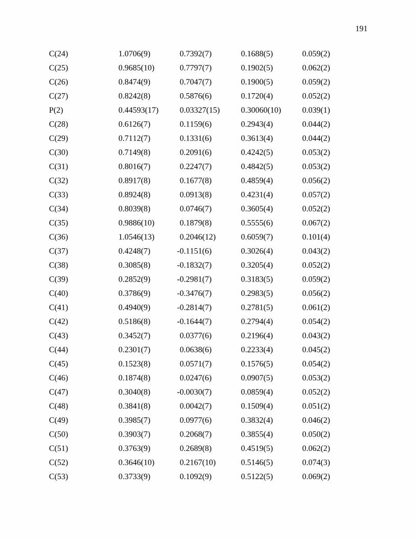
191
C(24) 1.0706(9) 0.7392(7) 0.1688(5) 0.059(2)
C(25) 0.9685(10) 0.7797(7) 0.1902(5) 0.062(2)
C(26) 0.8474(9) 0.7047(7) 0.1900(5) 0.059(2)
C(27) 0.8242(8) 0.5876(6) 0.1720(4) 0.052(2)
P(2) 0.44593(17) 0.03327(15) 0.30060(10) 0.039(1)
C(28) 0.6126(7) 0.1159(6) 0.2943(4) 0.044(2)
C(29) 0.7112(7) 0.1331(6) 0.3613(4) 0.044(2)
C(30) 0.7149(8) 0.2091(6) 0.4242(5) 0.053(2)
C(31) 0.8016(7) 0.2247(7) 0.4842(5) 0.053(2)
C(32) 0.8917(8) 0.1677(8) 0.4859(4) 0.056(2)
C(33) 0.8924(8) 0.0913(8) 0.4231(4) 0.057(2)
C(34) 0.8039(8) 0.0746(7) 0.3605(4) 0.052(2)
C(35) 0.9886(10) 0.1879(8) 0.5555(6) 0.067(2)
C(36) 1.0546(13) 0.2046(12) 0.6059(7) 0.101(4)
C(37) 0.4248(7) -0.1151(6) 0.3026(4) 0.043(2)
C(38) 0.3085(8) -0.1832(7) 0.3205(4) 0.052(2)
C(39) 0.2852(9) -0.2981(7) 0.3183(5) 0.059(2)
C(40) 0.3786(9) -0.3476(7) 0.2983(5) 0.056(2)
C(41) 0.4940(9) -0.2814(7) 0.2781(5) 0.061(2)
C(42) 0.5186(8) -0.1644(7) 0.2794(4) 0.054(2)
C(43) 0.3452(7) 0.0377(6) 0.2196(4) 0.043(2)
C(44) 0.2301(7) 0.0638(6) 0.2233(4) 0.045(2)
C(45) 0.1523(8) 0.0571(7) 0.1576(5) 0.054(2)
C(46) 0.1874(8) 0.0247(6) 0.0907(5) 0.053(2)
C(47) 0.3040(8) -0.0030(7) 0.0859(4) 0.052(2)
C(48) 0.3841(8) 0.0042(7) 0.1509(4) 0.051(2)
C(49) 0.3985(7) 0.0977(6) 0.3832(4) 0.046(2)
C(50) 0.3903(7) 0.2068(7) 0.3855(4) 0.050(2)
C(51) 0.3763(9) 0.2689(8) 0.4519(5) 0.062(2)
C(52) 0.3646(10) 0.2167(10) 0.5146(5) 0.074(3)
C(53) 0.3733(9) 0.1092(9) 0.5122(5) 0.069(2)

192
C(54) 0.3895(8) 0.0473(7) 0.4457(4) 0.053(2)
H(1A) 0.7474 0.3378 0.2133 0.055
H(1B) 0.8099 0.2406 0.1864 0.055
H(3) 0.8646 0.4934 0.3154 0.054
H(4) 1.0082 0.5485 0.4248 0.056
H(6) 1.1667 0.3024 0.3570 0.077
H(7) 1.0135 0.2417 0.2503 0.069
H(9) 1.3242 0.5190 0.5703 0.081
H(11) 0.6537 0.1946 0.0847 0.061
H(12) 0.4822 0.1347 -0.0132 0.066
H(13) 0.4665 0.2514 -0.0974 0.067
H(14) 0.6230 0.4304 -0.0878 0.081
H(15) 0.8044 0.4877 0.0032 0.070
H(17) 0.9185 0.2561 -0.0049 0.054
H(18) 1.0917 0.1971 -0.0433 0.065
H(19) 1.2924 0.2557 0.0330 0.072
H(20) 1.3237 0.3772 0.1446 0.070
H(21) 1.1506 0.4363 0.1860 0.062
H(23) 1.1153 0.5956 0.1336 0.060
H(24) 1.1552 0.7916 0.1680 0.071
H(25) 0.9844 0.8596 0.2049 0.075
H(26) 0.7778 0.7327 0.2024 0.071
H(27) 0.7401 0.5355 0.1741 0.063
H(28A) 0.6417 0.0777 0.2512 0.053
H(28B) 0.6135 0.1923 0.2845 0.053
H(30) 0.6550 0.2513 0.4252 0.063
H(31) 0.8004 0.2769 0.5269 0.064
H(33) 0.9536 0.0504 0.4230 0.068
H(34) 0.8059 0.0238 0.3173 0.062
H(36) 1.1127 0.2193 0.6502 0.122
H(38) 0.2438 -0.1499 0.3344 0.062
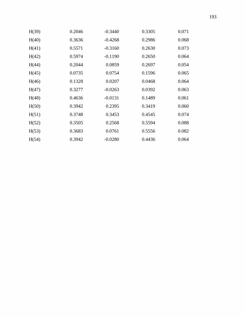
193
H(39) 0.2046 -0.3440 0.3305 0.071
H(40) 0.3636 -0.4268 0.2986 0.068
H(41) 0.5571 -0.3160 0.2630 0.073
H(42) 0.5974 -0.1190 0.2650 0.064
H(44) 0.2044 0.0859 0.2697 0.054
H(45) 0.0735 0.0754 0.1596 0.065
H(46) 0.1328 0.0207 0.0468 0.064
H(47) 0.3277 -0.0263 0.0392 0.063
H(48) 0.4636 -0.0131 0.1489 0.061
H(50) 0.3942 0.2395 0.3419 0.060
H(51) 0.3748 0.3453 0.4545 0.074
H(52) 0.3505 0.2568 0.5594 0.088
H(53) 0.3683 0.0761 0.5556 0.082
H(54) 0.3942 -0.0280 0.4436 0.064

194
Table 3. Anisotropic displacement parameters (Å2) for uvic1217.
The anisotropic displacement factor exponent takes the form:
-2π2[h
2a*
2U11 + ... + 2hka*b*U12]
U11 U22 U33 U23 U13 U12
Br(1) 0.0158(2) 0.0150(2) 0.0170(2) -0.0009(2) 0.0019(2) 0.0043(2)
Br(2) 0.0285(3) 0.0280(3) 0.0295(3) 0.0119(2) 0.0028(2) 0.0120(2)
P(1) 0.0417(9) 0.0315(8) 0.0380(9) 0.0056(7) 0.0037(7) 0.0058(7)
C(1) 0.057(4) 0.031(3) 0.048(4) 0.010(3) 0.010(3) 0.010(3)
C(2) 0.058(4) 0.032(3) 0.039(3) 0.008(3) 0.007(3) 0.010(3)
C(3) 0.050(4) 0.042(4) 0.045(4) 0.008(3) 0.007(3) 0.017(3)
C(4) 0.056(4) 0.044(4) 0.040(4) 0.002(3) 0.009(3) 0.019(3)
C(5) 0.066(5) 0.046(4) 0.041(4) 0.009(3) 0.011(3) 0.023(4)
C(6) 0.088(6) 0.062(5) 0.050(4) 0.000(4) -0.004(4) 0.042(5)
C(7) 0.088(6) 0.051(4) 0.041(4) 0.004(3) -0.001(4) 0.037(4)
C(8) 0.066(5) 0.058(5) 0.047(4) 0.004(4) 0.005(4) 0.030(4)
C(9) 0.080(6) 0.072(6) 0.055(5) -0.008(4) -0.010(4) 0.044(5)
C(10) 0.042(4) 0.042(4) 0.041(3) 0.006(3) 0.005(3) 0.013(3)
C(11) 0.051(4) 0.039(4) 0.058(4) 0.012(3) -0.002(3) 0.006(3)
C(12) 0.049(4) 0.041(4) 0.062(5) 0.005(3) -0.005(4) 0.003(3)
C(13) 0.045(4) 0.055(5) 0.057(5) 0.010(4) -0.002(3) 0.004(3)
C(14) 0.064(5) 0.063(5) 0.062(5) 0.028(4) -0.011(4) 0.000(4)
C(15) 0.055(5) 0.047(4) 0.058(5) 0.017(4) 0.000(4) -0.006(3)
C(16) 0.041(4) 0.040(4) 0.050(4) 0.013(3) 0.003(3) 0.004(3)
C(17) 0.045(4) 0.043(4) 0.049(4) 0.011(3) 0.006(3) 0.013(3)
C(18) 0.061(5) 0.053(4) 0.056(5) 0.019(4) 0.016(4) 0.023(4)
C(19) 0.057(5) 0.063(5) 0.071(6) 0.027(4) 0.016(4) 0.027(4)
C(20) 0.042(4) 0.060(5) 0.077(6) 0.030(4) 0.002(4) 0.016(4)
C(21) 0.048(4) 0.050(4) 0.054(4) 0.010(3) -0.002(3) 0.012(3)
C(22) 0.056(4) 0.032(3) 0.037(3) 0.005(3) 0.004(3) 0.009(3)

195
C(23) 0.054(4) 0.044(4) 0.043(4) 0.008(3) 0.000(3) 0.005(3)
C(24) 0.069(5) 0.039(4) 0.057(5) 0.013(3) -0.001(4) 0.001(4)
C(25) 0.086(6) 0.039(4) 0.060(5) 0.008(4) 0.011(4) 0.016(4)
C(26) 0.078(6) 0.040(4) 0.061(5) 0.012(4) 0.016(4) 0.018(4)
C(27) 0.058(4) 0.041(4) 0.058(4) 0.011(3) 0.012(4) 0.013(3)
P(2) 0.0425(9) 0.0395(9) 0.0400(9) 0.0115(7) 0.0103(7) 0.0153(7)
C(28) 0.049(4) 0.043(4) 0.044(4) 0.014(3) 0.014(3) 0.015(3)
C(29) 0.043(4) 0.042(4) 0.046(4) 0.012(3) 0.010(3) 0.010(3)
C(30) 0.048(4) 0.044(4) 0.062(5) -0.001(3) 0.007(4) 0.013(3)
C(31) 0.043(4) 0.060(5) 0.052(4) -0.001(4) 0.004(3) 0.015(3)
C(32) 0.048(4) 0.065(5) 0.049(4) 0.011(4) 0.002(3) 0.009(4)
C(33) 0.061(5) 0.070(5) 0.051(4) 0.009(4) 0.010(4) 0.036(4)
C(34) 0.056(4) 0.059(5) 0.047(4) 0.008(3) 0.009(3) 0.027(4)
C(35) 0.065(5) 0.068(6) 0.065(6) 0.003(4) 0.012(5) 0.019(4)
C(36) 0.093(8) 0.139(12) 0.064(7) -0.014(7) -0.010(6) 0.047(8)
C(37) 0.047(4) 0.040(3) 0.045(4) 0.013(3) 0.006(3) 0.015(3)
C(38) 0.051(4) 0.049(4) 0.056(4) 0.017(3) 0.008(3) 0.014(3)
C(39) 0.065(5) 0.045(4) 0.061(5) 0.015(4) 0.010(4) 0.007(4)
C(40) 0.074(5) 0.037(4) 0.059(5) 0.014(3) 0.006(4) 0.019(4)
C(41) 0.075(6) 0.046(4) 0.069(5) 0.013(4) 0.022(4) 0.027(4)
C(42) 0.062(5) 0.048(4) 0.056(4) 0.012(3) 0.016(4) 0.021(4)
C(43) 0.046(4) 0.043(4) 0.041(4) 0.013(3) 0.009(3) 0.012(3)
C(44) 0.041(4) 0.043(4) 0.051(4) 0.009(3) 0.005(3) 0.013(3)
C(45) 0.043(4) 0.046(4) 0.075(6) 0.012(4) 0.002(4) 0.016(3)
C(46) 0.054(4) 0.045(4) 0.055(4) 0.009(3) -0.004(4) 0.010(3)
C(47) 0.058(4) 0.054(4) 0.042(4) 0.014(3) 0.004(3) 0.013(4)
C(48) 0.053(4) 0.059(5) 0.044(4) 0.015(3) 0.007(3) 0.020(4)
C(49) 0.044(4) 0.053(4) 0.042(4) 0.011(3) 0.011(3) 0.015(3)
C(50) 0.053(4) 0.053(4) 0.049(4) 0.008(3) 0.008(3) 0.026(3)
C(51) 0.071(5) 0.068(5) 0.055(5) 0.004(4) 0.009(4) 0.036(5)
C(52) 0.086(7) 0.105(8) 0.047(5) 0.006(5) 0.021(4) 0.056(6)

196
C(53) 0.071(6) 0.090(7) 0.052(5) 0.020(5) 0.020(4) 0.031(5)
C(54) 0.058(5) 0.061(5) 0.046(4) 0.016(3) 0.016(3) 0.022(4)

197
Table 4. Bond lengths [Å] for uvic1217.
atom-atom distance atom-atom distance
P(1)-C(10) 1.790(7) P(1)-C(16) 1.795(8)
P(1)-C(22) 1.799(7) P(1)-C(1) 1.814(7)
C(1)-C(2) 1.508(10) C(2)-C(7) 1.377(11)
C(2)-C(3) 1.381(10) C(3)-C(4) 1.389(10)
C(4)-C(5) 1.375(10) C(5)-C(6) 1.401(11)
C(5)-C(8) 1.436(11) C(6)-C(7) 1.398(11)
C(8)-C(9) 1.194(12) C(10)-C(15) 1.386(10)
C(10)-C(11) 1.410(10) C(11)-C(12) 1.391(10)
C(12)-C(13) 1.368(11) C(13)-C(14) 1.375(11)
C(14)-C(15) 1.387(11) C(16)-C(21) 1.400(10)
C(16)-C(17) 1.401(10) C(17)-C(18) 1.382(10)
C(18)-C(19) 1.396(12) C(19)-C(20) 1.366(13)
C(20)-C(21) 1.399(11) C(22)-C(27) 1.387(11)
C(22)-C(23) 1.390(10) C(23)-C(24) 1.374(11)
C(24)-C(25) 1.409(13) C(25)-C(26) 1.357(12)
C(26)-C(27) 1.388(10) P(2)-C(43) 1.796(7)
P(2)-C(37) 1.797(7) P(2)-C(49) 1.803(7)
P(2)-C(28) 1.805(7) C(28)-C(29) 1.513(10)
C(29)-C(30) 1.378(10) C(29)-C(34) 1.407(10)
C(30)-C(31) 1.344(11) C(31)-C(32) 1.371(11)
C(32)-C(33) 1.391(11) C(32)-C(35) 1.531(13)
C(33)-C(34) 1.389(11) C(35)-C(36) 1.078(14)
C(37)-C(38) 1.381(10) C(37)-C(42) 1.401(10)
C(38)-C(39) 1.368(11) C(39)-C(40) 1.382(12)
C(40)-C(41) 1.383(12) C(41)-C(42) 1.395(11)
C(43)-C(44) 1.384(10) C(43)-C(48) 1.414(10)
C(44)-C(45) 1.396(11) C(45)-C(46) 1.363(12)

198
C(46)-C(47) 1.411(11) C(47)-C(48) 1.397(10)
C(49)-C(50) 1.383(10) C(49)-C(54) 1.386(10)
C(50)-C(51) 1.397(11) C(51)-C(52) 1.403(13)
C(52)-C(53) 1.365(14) C(53)-C(54) 1.406(12)
C(1)-H(1A) 0.9900 C(1)-H(1B) 0.9900
C(3)-H(3) 0.9500 C(4)-H(4) 0.9500
C(6)-H(6) 0.9500 C(7)-H(7) 0.9500
C(9)-H(9) 0.9500 C(11)-H(11) 0.9500
C(12)-H(12) 0.9500 C(13)-H(13) 0.9500
C(14)-H(14) 0.9500 C(15)-H(15) 0.9500
C(17)-H(17) 0.9500 C(18)-H(18) 0.9500
C(19)-H(19) 0.9500 C(20)-H(20) 0.9500
C(21)-H(21) 0.9500 C(23)-H(23) 0.9500
C(24)-H(24) 0.9500 C(25)-H(25) 0.9500
C(26)-H(26) 0.9500 C(27)-H(27) 0.9500
C(28)-H(28A) 0.9900 C(28)-H(28B) 0.9900
C(30)-H(30) 0.9500 C(31)-H(31) 0.9500
C(33)-H(33) 0.9500 C(34)-H(34) 0.9500
C(36)-H(36) 0.9500 C(38)-H(38) 0.9500
C(39)-H(39) 0.9500 C(40)-H(40) 0.9500
C(41)-H(41) 0.9500 C(42)-H(42) 0.9500
C(44)-H(44) 0.9500 C(45)-H(45) 0.9500
C(46)-H(46) 0.9500 C(47)-H(47) 0.9500
C(48)-H(48) 0.9500 C(50)-H(50) 0.9500
C(51)-H(51) 0.9500 C(52)-H(52) 0.9500
C(53)-H(53) 0.9500 C(54)-H(54) 0.9500
Symmetry transformations used to generate equivalent atoms:
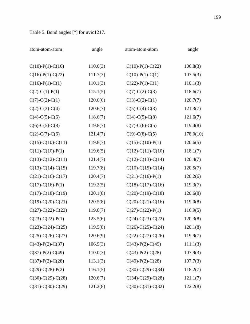
199
Table 5. Bond angles [°] for uvic1217.
atom-atom-atom angle atom-atom-atom angle
C(10)-P(1)-C(16) 110.6(3) C(10)-P(1)-C(22) 106.8(3)
C(16)-P(1)-C(22) 111.7(3) C(10)-P(1)-C(1) 107.5(3)
C(16)-P(1)-C(1) 110.1(3) C(22)-P(1)-C(1) 110.1(3)
C(2)-C(1)-P(1) 115.1(5) C(7)-C(2)-C(3) 118.6(7)
C(7)-C(2)-C(1) 120.6(6) C(3)-C(2)-C(1) 120.7(7)
C(2)-C(3)-C(4) 120.6(7) C(5)-C(4)-C(3) 121.3(7)
C(4)-C(5)-C(6) 118.6(7) C(4)-C(5)-C(8) 121.6(7)
C(6)-C(5)-C(8) 119.8(7) C(7)-C(6)-C(5) 119.4(8)
C(2)-C(7)-C(6) 121.4(7) C(9)-C(8)-C(5) 178.0(10)
C(15)-C(10)-C(11) 119.8(7) C(15)-C(10)-P(1) 120.6(5)
C(11)-C(10)-P(1) 119.6(5) C(12)-C(11)-C(10) 118.1(7)
C(13)-C(12)-C(11) 121.4(7) C(12)-C(13)-C(14) 120.4(7)
C(13)-C(14)-C(15) 119.7(8) C(10)-C(15)-C(14) 120.5(7)
C(21)-C(16)-C(17) 120.4(7) C(21)-C(16)-P(1) 120.2(6)
C(17)-C(16)-P(1) 119.2(5) C(18)-C(17)-C(16) 119.3(7)
C(17)-C(18)-C(19) 120.1(8) C(20)-C(19)-C(18) 120.6(8)
C(19)-C(20)-C(21) 120.5(8) C(20)-C(21)-C(16) 119.0(8)
C(27)-C(22)-C(23) 119.6(7) C(27)-C(22)-P(1) 116.9(5)
C(23)-C(22)-P(1) 123.5(6) C(24)-C(23)-C(22) 120.3(8)
C(23)-C(24)-C(25) 119.5(8) C(26)-C(25)-C(24) 120.1(8)
C(25)-C(26)-C(27) 120.6(9) C(22)-C(27)-C(26) 119.9(7)
C(43)-P(2)-C(37) 106.9(3) C(43)-P(2)-C(49) 111.1(3)
C(37)-P(2)-C(49) 110.0(3) C(43)-P(2)-C(28) 107.9(3)
C(37)-P(2)-C(28) 113.1(3) C(49)-P(2)-C(28) 107.7(3)
C(29)-C(28)-P(2) 116.1(5) C(30)-C(29)-C(34) 118.2(7)
C(30)-C(29)-C(28) 120.6(7) C(34)-C(29)-C(28) 121.1(7)
C(31)-C(30)-C(29) 121.2(8) C(30)-C(31)-C(32) 122.2(8)

200
C(31)-C(32)-C(33) 118.4(7) C(31)-C(32)-C(35) 120.4(8)
C(33)-C(32)-C(35) 121.2(8) C(34)-C(33)-C(32) 120.2(8)
C(33)-C(34)-C(29) 119.8(7) C(36)-C(35)-C(32) 177.4(12)
C(38)-C(37)-C(42) 119.9(7) C(38)-C(37)-P(2) 118.9(6)
C(42)-C(37)-P(2) 120.9(6) C(39)-C(38)-C(37) 120.8(8)
C(38)-C(39)-C(40) 120.2(8) C(39)-C(40)-C(41) 119.8(7)
C(40)-C(41)-C(42) 120.6(8) C(41)-C(42)-C(37) 118.6(7)
C(44)-C(43)-C(48) 121.1(7) C(44)-C(43)-P(2) 122.3(5)
C(48)-C(43)-P(2) 116.4(6) C(43)-C(44)-C(45) 118.8(7)
C(46)-C(45)-C(44) 121.3(7) C(45)-C(46)-C(47) 120.7(7)
C(48)-C(47)-C(46) 119.1(7) C(47)-C(48)-C(43) 119.0(7)
C(50)-C(49)-C(54) 120.9(7) C(50)-C(49)-P(2) 117.3(5)
C(54)-C(49)-P(2) 121.2(6) C(49)-C(50)-C(51) 119.9(8)
C(50)-C(51)-C(52) 118.9(8) C(53)-C(52)-C(51) 120.9(8)
C(52)-C(53)-C(54) 120.2(8) C(49)-C(54)-C(53) 119.1(8)
C(2)-C(1)-H(1A) 108.5 P(1)-C(1)-H(1A) 108.5
C(2)-C(1)-H(1B) 108.5 P(1)-C(1)-H(1B) 108.5
H(1A)-C(1)-H(1B) 107.5 C(2)-C(3)-H(3) 119.7
C(4)-C(3)-H(3) 119.7 C(5)-C(4)-H(4) 119.4
C(3)-C(4)-H(4) 119.4 C(7)-C(6)-H(6) 120.3
C(5)-C(6)-H(6) 120.3 C(2)-C(7)-H(7) 119.3
C(6)-C(7)-H(7) 119.3 C(8)-C(9)-H(9) 180.0
C(12)-C(11)-H(11) 120.9 C(10)-C(11)-H(11) 120.9
C(13)-C(12)-H(12) 119.3 C(11)-C(12)-H(12) 119.3
C(12)-C(13)-H(13) 119.8 C(14)-C(13)-H(13) 119.8
C(13)-C(14)-H(14) 120.2 C(15)-C(14)-H(14) 120.2
C(10)-C(15)-H(15) 119.8 C(14)-C(15)-H(15) 119.8
C(18)-C(17)-H(17) 120.3 C(16)-C(17)-H(17) 120.3
C(17)-C(18)-H(18) 119.9 C(19)-C(18)-H(18) 119.9
C(20)-C(19)-H(19) 119.7 C(18)-C(19)-H(19) 119.7
C(19)-C(20)-H(20) 119.8 C(21)-C(20)-H(20) 119.8
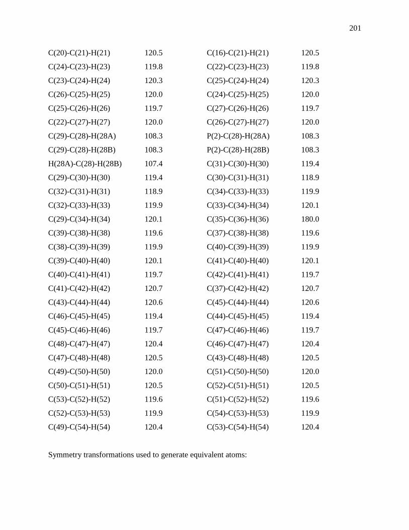
201
C(20)-C(21)-H(21) 120.5 C(16)-C(21)-H(21) 120.5
C(24)-C(23)-H(23) 119.8 C(22)-C(23)-H(23) 119.8
C(23)-C(24)-H(24) 120.3 C(25)-C(24)-H(24) 120.3
C(26)-C(25)-H(25) 120.0 C(24)-C(25)-H(25) 120.0
C(25)-C(26)-H(26) 119.7 C(27)-C(26)-H(26) 119.7
C(22)-C(27)-H(27) 120.0 C(26)-C(27)-H(27) 120.0
C(29)-C(28)-H(28A) 108.3 P(2)-C(28)-H(28A) 108.3
C(29)-C(28)-H(28B) 108.3 P(2)-C(28)-H(28B) 108.3
H(28A)-C(28)-H(28B) 107.4 C(31)-C(30)-H(30) 119.4
C(29)-C(30)-H(30) 119.4 C(30)-C(31)-H(31) 118.9
C(32)-C(31)-H(31) 118.9 C(34)-C(33)-H(33) 119.9
C(32)-C(33)-H(33) 119.9 C(33)-C(34)-H(34) 120.1
C(29)-C(34)-H(34) 120.1 C(35)-C(36)-H(36) 180.0
C(39)-C(38)-H(38) 119.6 C(37)-C(38)-H(38) 119.6
C(38)-C(39)-H(39) 119.9 C(40)-C(39)-H(39) 119.9
C(39)-C(40)-H(40) 120.1 C(41)-C(40)-H(40) 120.1
C(40)-C(41)-H(41) 119.7 C(42)-C(41)-H(41) 119.7
C(41)-C(42)-H(42) 120.7 C(37)-C(42)-H(42) 120.7
C(43)-C(44)-H(44) 120.6 C(45)-C(44)-H(44) 120.6
C(46)-C(45)-H(45) 119.4 C(44)-C(45)-H(45) 119.4
C(45)-C(46)-H(46) 119.7 C(47)-C(46)-H(46) 119.7
C(48)-C(47)-H(47) 120.4 C(46)-C(47)-H(47) 120.4
C(47)-C(48)-H(48) 120.5 C(43)-C(48)-H(48) 120.5
C(49)-C(50)-H(50) 120.0 C(51)-C(50)-H(50) 120.0
C(50)-C(51)-H(51) 120.5 C(52)-C(51)-H(51) 120.5
C(53)-C(52)-H(52) 119.6 C(51)-C(52)-H(52) 119.6
C(52)-C(53)-H(53) 119.9 C(54)-C(53)-H(53) 119.9
C(49)-C(54)-H(54) 120.4 C(53)-C(54)-H(54) 120.4
Symmetry transformations used to generate equivalent atoms:
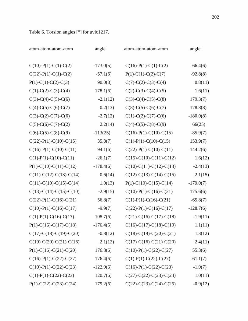
202
Table 6. Torsion angles [°] for uvic1217.
atom-atom-atom-atom angle atom-atom-atom-atom angle
C(10)-P(1)-C(1)-C(2) -173.0(5) C(16)-P(1)-C(1)-C(2) 66.4(6)
C(22)-P(1)-C(1)-C(2) -57.1(6) P(1)-C(1)-C(2)-C(7) -92.8(8)
P(1)-C(1)-C(2)-C(3) 90.0(8) C(7)-C(2)-C(3)-C(4) 0.8(11)
C(1)-C(2)-C(3)-C(4) 178.1(6) C(2)-C(3)-C(4)-C(5) 1.6(11)
C(3)-C(4)-C(5)-C(6) -2.1(12) C(3)-C(4)-C(5)-C(8) 179.3(7)
C(4)-C(5)-C(6)-C(7) 0.2(13) C(8)-C(5)-C(6)-C(7) 178.8(8)
C(3)-C(2)-C(7)-C(6) -2.7(12) C(1)-C(2)-C(7)-C(6) -180.0(8)
C(5)-C(6)-C(7)-C(2) 2.2(14) C(4)-C(5)-C(8)-C(9) 66(25)
C(6)-C(5)-C(8)-C(9) -113(25) C(16)-P(1)-C(10)-C(15) -85.9(7)
C(22)-P(1)-C(10)-C(15) 35.8(7) C(1)-P(1)-C(10)-C(15) 153.9(7)
C(16)-P(1)-C(10)-C(11) 94.1(6) C(22)-P(1)-C(10)-C(11) -144.2(6)
C(1)-P(1)-C(10)-C(11) -26.1(7) C(15)-C(10)-C(11)-C(12) 1.6(12)
P(1)-C(10)-C(11)-C(12) -178.4(6) C(10)-C(11)-C(12)-C(13) -2.4(13)
C(11)-C(12)-C(13)-C(14) 0.6(14) C(12)-C(13)-C(14)-C(15) 2.1(15)
C(11)-C(10)-C(15)-C(14) 1.0(13) P(1)-C(10)-C(15)-C(14) -179.0(7)
C(13)-C(14)-C(15)-C(10) -2.9(15) C(10)-P(1)-C(16)-C(21) 175.6(6)
C(22)-P(1)-C(16)-C(21) 56.8(7) C(1)-P(1)-C(16)-C(21) -65.8(7)
C(10)-P(1)-C(16)-C(17) -9.9(7) C(22)-P(1)-C(16)-C(17) -128.7(6)
C(1)-P(1)-C(16)-C(17) 108.7(6) C(21)-C(16)-C(17)-C(18) -1.9(11)
P(1)-C(16)-C(17)-C(18) -176.4(5) C(16)-C(17)-C(18)-C(19) 1.1(11)
C(17)-C(18)-C(19)-C(20) -0.8(12) C(18)-C(19)-C(20)-C(21) 1.3(12)
C(19)-C(20)-C(21)-C(16) -2.1(12) C(17)-C(16)-C(21)-C(20) 2.4(11)
P(1)-C(16)-C(21)-C(20) 176.8(6) C(10)-P(1)-C(22)-C(27) 55.3(6)
C(16)-P(1)-C(22)-C(27) 176.4(6) C(1)-P(1)-C(22)-C(27) -61.1(7)
C(10)-P(1)-C(22)-C(23) -122.9(6) C(16)-P(1)-C(22)-C(23) -1.9(7)
C(1)-P(1)-C(22)-C(23) 120.7(6) C(27)-C(22)-C(23)-C(24) 1.0(11)
P(1)-C(22)-C(23)-C(24) 179.2(6) C(22)-C(23)-C(24)-C(25) -0.9(12)
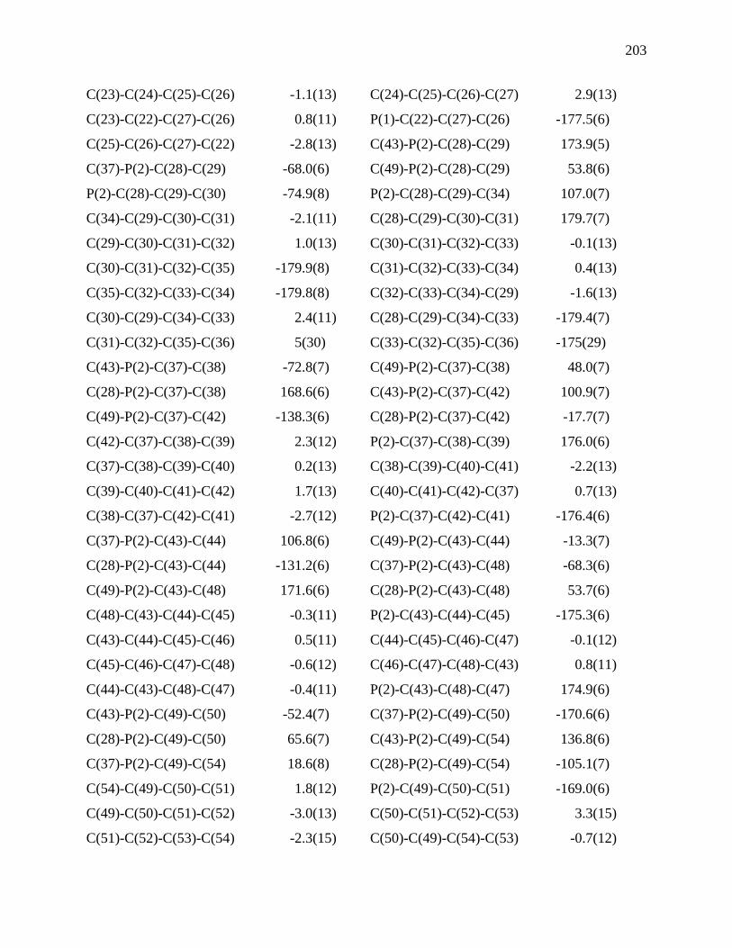
203
C(23)-C(24)-C(25)-C(26) -1.1(13) C(24)-C(25)-C(26)-C(27) 2.9(13)
C(23)-C(22)-C(27)-C(26) 0.8(11) P(1)-C(22)-C(27)-C(26) -177.5(6)
C(25)-C(26)-C(27)-C(22) -2.8(13) C(43)-P(2)-C(28)-C(29) 173.9(5)
C(37)-P(2)-C(28)-C(29) -68.0(6) C(49)-P(2)-C(28)-C(29) 53.8(6)
P(2)-C(28)-C(29)-C(30) -74.9(8) P(2)-C(28)-C(29)-C(34) 107.0(7)
C(34)-C(29)-C(30)-C(31) -2.1(11) C(28)-C(29)-C(30)-C(31) 179.7(7)
C(29)-C(30)-C(31)-C(32) 1.0(13) C(30)-C(31)-C(32)-C(33) -0.1(13)
C(30)-C(31)-C(32)-C(35) -179.9(8) C(31)-C(32)-C(33)-C(34) 0.4(13)
C(35)-C(32)-C(33)-C(34) -179.8(8) C(32)-C(33)-C(34)-C(29) -1.6(13)
C(30)-C(29)-C(34)-C(33) 2.4(11) C(28)-C(29)-C(34)-C(33) -179.4(7)
C(31)-C(32)-C(35)-C(36) 5(30) C(33)-C(32)-C(35)-C(36) -175(29)
C(43)-P(2)-C(37)-C(38) -72.8(7) C(49)-P(2)-C(37)-C(38) 48.0(7)
C(28)-P(2)-C(37)-C(38) 168.6(6) C(43)-P(2)-C(37)-C(42) 100.9(7)
C(49)-P(2)-C(37)-C(42) -138.3(6) C(28)-P(2)-C(37)-C(42) -17.7(7)
C(42)-C(37)-C(38)-C(39) 2.3(12) P(2)-C(37)-C(38)-C(39) 176.0(6)
C(37)-C(38)-C(39)-C(40) 0.2(13) C(38)-C(39)-C(40)-C(41) -2.2(13)
C(39)-C(40)-C(41)-C(42) 1.7(13) C(40)-C(41)-C(42)-C(37) 0.7(13)
C(38)-C(37)-C(42)-C(41) -2.7(12) P(2)-C(37)-C(42)-C(41) -176.4(6)
C(37)-P(2)-C(43)-C(44) 106.8(6) C(49)-P(2)-C(43)-C(44) -13.3(7)
C(28)-P(2)-C(43)-C(44) -131.2(6) C(37)-P(2)-C(43)-C(48) -68.3(6)
C(49)-P(2)-C(43)-C(48) 171.6(6) C(28)-P(2)-C(43)-C(48) 53.7(6)
C(48)-C(43)-C(44)-C(45) -0.3(11) P(2)-C(43)-C(44)-C(45) -175.3(6)
C(43)-C(44)-C(45)-C(46) 0.5(11) C(44)-C(45)-C(46)-C(47) -0.1(12)
C(45)-C(46)-C(47)-C(48) -0.6(12) C(46)-C(47)-C(48)-C(43) 0.8(11)
C(44)-C(43)-C(48)-C(47) -0.4(11) P(2)-C(43)-C(48)-C(47) 174.9(6)
C(43)-P(2)-C(49)-C(50) -52.4(7) C(37)-P(2)-C(49)-C(50) -170.6(6)
C(28)-P(2)-C(49)-C(50) 65.6(7) C(43)-P(2)-C(49)-C(54) 136.8(6)
C(37)-P(2)-C(49)-C(54) 18.6(8) C(28)-P(2)-C(49)-C(54) -105.1(7)
C(54)-C(49)-C(50)-C(51) 1.8(12) P(2)-C(49)-C(50)-C(51) -169.0(6)
C(49)-C(50)-C(51)-C(52) -3.0(13) C(50)-C(51)-C(52)-C(53) 3.3(15)
C(51)-C(52)-C(53)-C(54) -2.3(15) C(50)-C(49)-C(54)-C(53) -0.7(12)

204
P(2)-C(49)-C(54)-C(53) 169.7(7) C(52)-C(53)-C(54)-C(49) 1.0(14)
Symmetry transformations used to generate equivalent atoms:

205
Appendix F: Supporting data for Weller’s hydrogenation
Figure SI 1. ln[x] vs time plots for alkene hydrogenation by H2 (red) and D2 (blue). First order rate constants are kH = 0.9±0.1 s
-1 and kD = 0.44±0.01 s
-1.
Figure SI 2 Final product and a mix of [RhP2]+ and [RhP2(FPh)]
+ when hydrogenation in nearly finished.
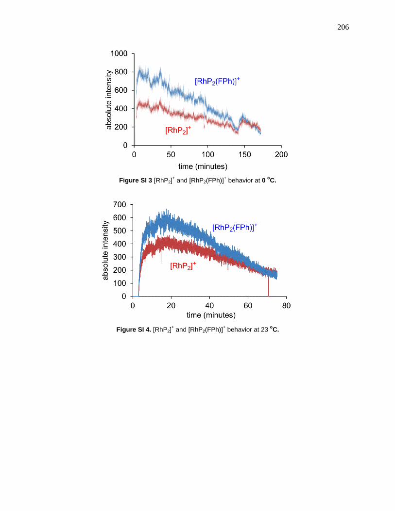
206
Figure SI 3 [RhP2]+ and [RhP2(FPh)]
+ behavior at 0
oC.
Figure SI 4. [RhP2]+ and [RhP2(FPh)]
+ behavior at 23
oC.
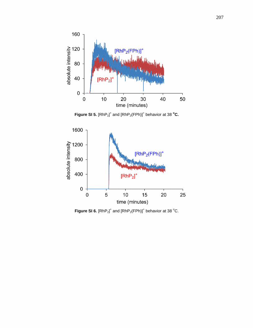
207
Figure SI 5. [RhP2]+ and [RhP2(FPh)]
+ behavior at 38
oC.
Figure SI 6. [RhP2]+ and [RhP2(FPh)]
+ behavior at 38
oC.

208
Figure SI 7 Addition of NEt3 leads to the disappearance of [RhP2]+ and the appearance of [HNEt3]
+
209
Appendix G: Crystal data and structure refinement for PPh3P(CH2)5CH3.
Identification code uvic1302
Empirical formula C24H28F6P2
Formula weight 492.40
Temperature 120(2) K
Wavelength 0.71073 Å
Crystal system Orthorhombic
Space group Pbca
Unit cell dimensions a = 13.3757(15) Å α = 90°
b = 17.979(2) Å β = 90°
c = 19.568(2) Å γ = 90°
Volume 4705.9(9) Å3
Z 8
Density (calculated) 1.390 g.cm-3
Absorption coefficient (μ) 0.242 mm-1
F(000) 2048
Crystal color, habit colorless, tablet
Crystal size 0.230 × 0.180 × 0.070 mm3
θ range for data collection 2.081 to 26.481°
Index ranges -16 ≤ h ≤ 16, -22 ≤ k ≤ 22, -24 ≤ l ≤ 24
Reflections collected 55595
Independent reflections 4858 [Rint = 0.0561]
Completeness to θ = 25.242° 100.0 %
Absorption correction Numerical
Max. and min. transmission 1.0000 and 0.8375
Refinement method Full-matrix least-squares on F2
Data / restraints / parameters 4858 / 0 / 306
Goodness-of-fit on F2 1.044
Final R indices [I>2σ(I)] R1 = 0.0434, wR2 = 0.1005
R indices (all data) R1 = 0.0637, wR2 = 0.1091
Extinction coefficient n/a
Largest diff. peak and hole 0.528 and -0.451 e–.Å
-3

210
Table S 2. Atomic coordinates and equivalent isotropic displacement parameters (Å2)
for uvic1302_x. U(eq) is defined as one third of the trace of the orthogonalized Uij tensor.
x y z U(eq)
P(1) 0.34382(4) 0.24259(3) 0.34052(3) 0.019(1)
C(1) 0.33641(15) 0.26159(12) 0.25052(11) 0.025(1)
C(2) 0.42290(16) 0.30731(13) 0.22289(11) 0.029(1)
C(3) 0.41580(15) 0.31619(13) 0.14559(11) 0.028(1)
C(4) 0.50425(16) 0.35820(13) 0.11677(11) 0.029(1)
C(5) 0.49729(16) 0.37350(12) 0.03995(11) 0.031(1)
C(6) 0.41137(19) 0.42259(15) 0.02027(12) 0.039(1)
C(7) 0.24166(14) 0.18222(11) 0.36305(10) 0.023(1)
C(8) 0.20236(17) 0.18428(13) 0.42860(12) 0.032(1)
C(9) 0.12354(17) 0.13798(14) 0.44630(13) 0.038(1)
C(10) 0.08302(16) 0.09057(13) 0.39891(13) 0.034(1)
C(11) 0.12095(19) 0.08831(15) 0.33387(13) 0.042(1)
C(12) 0.20049(18) 0.13332(14) 0.31552(12) 0.036(1)
C(13) 0.33259(14) 0.32456(11) 0.39177(10) 0.021(1)
C(14) 0.27700(15) 0.38445(12) 0.36762(11) 0.026(1)
C(15) 0.25770(17) 0.44382(13) 0.41103(12) 0.033(1)
C(16) 0.29278(17) 0.44357(13) 0.47731(13) 0.034(1)
C(17) 0.34822(15) 0.38416(13) 0.50117(12) 0.031(1)
C(18) 0.36825(14) 0.32465(12) 0.45880(11) 0.025(1)
C(19) 0.46246(14) 0.19939(11) 0.35605(10) 0.020(1)
C(20) 0.47263(15) 0.12343(12) 0.34363(11) 0.025(1)
C(21) 0.56572(17) 0.09040(13) 0.34961(11) 0.030(1)
C(22) 0.64802(16) 0.13271(13) 0.36845(11) 0.031(1)
C(23) 0.63811(15) 0.20790(13) 0.37994(11) 0.028(1)
C(24) 0.54581(14) 0.24231(12) 0.37306(10) 0.023(1)
P(2) -0.14461(4) -0.03949(3) 0.31318(3) 0.028(1)
F(1) -0.15447(10) -0.12416(7) 0.28999(8) 0.044(1)
F(2) -0.13410(11) 0.04629(9) 0.33459(10) 0.063(1)
F(3) -0.25964(12) -0.02943(11) 0.29599(12) 0.063(1)
F(4) -0.03131(13) -0.05419(11) 0.33122(15) 0.070(1)
F(5) -0.1174(2) -0.01839(11) 0.23812(10) 0.074(1)
F(6) -0.1737(2) -0.06455(19) 0.38772(11) 0.105(1)
F(3A) -0.2397(8) -0.0306(6) 0.3595(5) 0.041(3)
F(4A) -0.0417(7) -0.0289(5) 0.2722(5) 0.034(3)
F(5A) -0.2076(8) -0.0069(5) 0.2513(5) 0.038(3)
F(6A) -0.0841(8) -0.0519(5) 0.3794(5) 0.036(3)
H(1A) 0.3339 0.2137 0.2255 0.030
H(1B) 0.2732 0.2884 0.2412 0.030
H(2A) 0.4868 0.2826 0.2347 0.034
H(2B) 0.4225 0.3570 0.2446 0.034
H(3A) 0.4124 0.2664 0.1241 0.034
H(3B) 0.3535 0.3431 0.1341 0.034

211
H(4A) 0.5658 0.3293 0.1258 0.035
H(4B) 0.5104 0.4062 0.1411 0.035
H(5A) 0.5603 0.3971 0.0247 0.037
H(5B) 0.4908 0.3255 0.0156 0.037
H(6A) 0.4113 0.4298 -0.0294 0.058
H(6B) 0.4182 0.4709 0.0430 0.058
H(6C) 0.3485 0.3992 0.0343 0.058
H(8) 0.2295 0.2175 0.4615 0.039
H(9) 0.0975 0.1391 0.4915 0.045
H(10) 0.0287 0.0593 0.4112 0.041
H(11) 0.0924 0.0556 0.3011 0.051
H(12) 0.2270 0.1309 0.2705 0.044
H(14) 0.2526 0.3847 0.3220 0.032
H(15) 0.2200 0.4850 0.3949 0.040
H(16) 0.2788 0.4844 0.5066 0.041
H(17) 0.3726 0.3843 0.5468 0.037
H(18) 0.4063 0.2838 0.4752 0.030
H(20) 0.4161 0.0945 0.3311 0.030
H(21) 0.5733 0.0387 0.3408 0.036
H(22) 0.7115 0.1097 0.3734 0.038
H(23) 0.6949 0.2364 0.3927 0.034
H(24) 0.5394 0.2944 0.3798 0.027

212
Table S 3. Anisotropic displacement parameters (Å2) for uvic1302_x.
The anisotropic displacement factor exponent takes the form:
-2π2[h
2a*
2U11 + ... + 2hka*b*U12]
U11 U22 U33 U23 U13 U12
P(1) 0.0166(2) 0.0245(3) 0.0171(2) 0.0001(2) -0.0006(2) 0.0018(2)
C(1) 0.0233(9) 0.0309(11) 0.0210(10) -0.0005(9) -0.0022(8) 0.0028(9)
C(2) 0.0279(11) 0.0323(12) 0.0253(11) 0.0011(9) -0.0033(9) -0.0042(9)
C(3) 0.0253(10) 0.0361(12) 0.0226(11) 0.0028(9) 0.0007(9) -0.0031(9)
C(4) 0.0269(11) 0.0334(12) 0.0272(12) -0.0013(10) 0.0001(9) -0.0023(9)
C(5) 0.0339(12) 0.0320(12) 0.0256(11) -0.0063(10) 0.0099(10) -0.0103(10)
C(6) 0.0482(15) 0.0463(15) 0.0223(12) 0.0031(11) 0.0016(11) -0.0029(12)
C(7) 0.0182(9) 0.0251(11) 0.0240(11) -0.0003(9) -0.0021(8) 0.0012(8)
C(8) 0.0320(12) 0.0356(13) 0.0287(12) -0.0093(10) 0.0060(10) -0.0066(10)
C(9) 0.0337(12) 0.0416(14) 0.0379(14) -0.0050(11) 0.0143(11) -0.0062(11)
C(10) 0.0200(10) 0.0370(13) 0.0458(15) 0.0002(11) 0.0027(10) -0.0064(9)
C(11) 0.0392(13) 0.0508(16) 0.0372(14) -0.0024(12) -0.0068(11) -0.0208(12)
C(12) 0.0383(13) 0.0473(15) 0.0232(12) -0.0029(11) -0.0007(10) -0.0143(11)
C(13) 0.0170(9) 0.0233(10) 0.0222(10) -0.0011(8) 0.0010(8) -0.0010(8)
C(14) 0.0229(10) 0.0284(11) 0.0281(11) 0.0036(9) -0.0004(9) 0.0021(9)
C(15) 0.0324(12) 0.0249(11) 0.0423(14) 0.0016(10) 0.0035(11) 0.0059(9)
C(16) 0.0306(11) 0.0291(12) 0.0420(14) -0.0107(11) 0.0083(10) -0.0020(10)
C(17) 0.0240(10) 0.0402(13) 0.0276(12) -0.0078(10) 0.0006(9) -0.0030(10)
C(18) 0.0192(9) 0.0321(12) 0.0239(11) -0.0019(9) 0.0007(8) 0.0028(8)
C(19) 0.0180(9) 0.0274(11) 0.0154(10) 0.0045(8) 0.0019(8) 0.0027(8)
C(20) 0.0256(10) 0.0274(11) 0.0232(11) 0.0022(9) 0.0030(9) 0.0008(9)
C(21) 0.0359(12) 0.0272(12) 0.0278(12) 0.0044(10) 0.0065(10) 0.0095(9)
C(22) 0.0243(10) 0.0470(14) 0.0224(11) 0.0061(10) 0.0051(9) 0.0141(10)
C(23) 0.0173(10) 0.0454(14) 0.0216(11) 0.0021(10) 0.0013(8) 0.0004(9)
C(24) 0.0215(9) 0.0280(11) 0.0186(10) 0.0021(9) 0.0027(8) 0.0006(8)
P(2) 0.0182(3) 0.0371(3) 0.0287(3) -0.0072(2) -0.0003(2) 0.0001(2)
F(1) 0.0399(8) 0.0276(7) 0.0643(10) 0.0051(7) -0.0189(7) -0.0074(6)
F(2) 0.0376(8) 0.0538(10) 0.0987(14) -0.0471(10) -0.0153(9) 0.0138(7)
F(3) 0.0236(9) 0.0592(13) 0.1064(19) -0.0272(12) -0.0191(10) 0.0091(8)
F(4) 0.0238(9) 0.0459(11) 0.141(2) -0.0357(13) -0.0284(12) 0.0053(8)
F(5) 0.129(2) 0.0443(11) 0.0480(13) 0.0083(9) 0.0364(14) -0.0150(13)
F(6) 0.111(2) 0.178(3) 0.0247(11) 0.0021(14) 0.0129(12) -0.016(2)
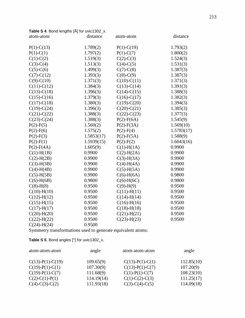
213
Table S 4. Bond lengths [Å] for uvic1302_x.
atom-atom distance atom-atom distance
P(1)-C(13) 1.789(2) P(1)-C(19) 1.793(2)
P(1)-C(1) 1.797(2) P(1)-C(7) 1.800(2)
C(1)-C(2) 1.519(3) C(2)-C(3) 1.524(3)
C(3)-C(4) 1.513(3) C(4)-C(5) 1.531(3)
C(5)-C(6) 1.499(3) C(7)-C(8) 1.387(3)
C(7)-C(12) 1.393(3) C(8)-C(9) 1.387(3)
C(9)-C(10) 1.371(3) C(10)-C(11) 1.371(3)
C(11)-C(12) 1.384(3) C(13)-C(14) 1.391(3)
C(13)-C(18) 1.396(3) C(14)-C(15) 1.388(3)
C(15)-C(16) 1.379(3) C(16)-C(17) 1.382(3)
C(17)-C(18) 1.380(3) C(19)-C(20) 1.394(3)
C(19)-C(24) 1.396(3) C(20)-C(21) 1.385(3)
C(21)-C(22) 1.388(3) C(22)-C(23) 1.377(3)
C(23)-C(24) 1.388(3) P(2)-F(6A) 1.545(9)
P(2)-F(5) 1.560(2) P(2)-F(3A) 1.569(10)
P(2)-F(6) 1.575(2) P(2)-F(4) 1.5783(17)
P(2)-F(3) 1.5853(17) P(2)-F(5A) 1.588(9)
P(2)-F(1) 1.5939(15) P(2)-F(2) 1.6043(16)
P(2)-F(4A) 1.605(9) C(1)-H(1A) 0.9900
C(1)-H(1B) 0.9900 C(2)-H(2A) 0.9900
C(2)-H(2B) 0.9900 C(3)-H(3A) 0.9900
C(3)-H(3B) 0.9900 C(4)-H(4A) 0.9900
C(4)-H(4B) 0.9900 C(5)-H(5A) 0.9900
C(5)-H(5B) 0.9900 C(6)-H(6A) 0.9800
C(6)-H(6B) 0.9800 C(6)-H(6C) 0.9800
C(8)-H(8) 0.9500 C(9)-H(9) 0.9500
C(10)-H(10) 0.9500 C(11)-H(11) 0.9500
C(12)-H(12) 0.9500 C(14)-H(14) 0.9500
C(15)-H(15) 0.9500 C(16)-H(16) 0.9500
C(17)-H(17) 0.9500 C(18)-H(18) 0.9500
C(20)-H(20) 0.9500 C(21)-H(21) 0.9500
C(22)-H(22) 0.9500 C(23)-H(23) 0.9500
C(24)-H(24) 0.9500
Symmetry transformations used to generate equivalent atoms: Table S 5. Bond angles [°] for uvic1302_x.
atom-atom-atom angle atom-atom-atom angle
C(13)-P(1)-C(19) 109.65(9) C(13)-P(1)-C(1) 112.85(10)
C(19)-P(1)-C(1) 107.30(9) C(13)-P(1)-C(7) 107.20(9)
C(19)-P(1)-C(7) 111.68(9) C(1)-P(1)-C(7) 108.23(10)
C(2)-C(1)-P(1) 114.19(14) C(1)-C(2)-C(3) 111.25(17)
C(4)-C(3)-C(2) 111.93(18) C(3)-C(4)-C(5) 114.09(18)

214
C(6)-C(5)-C(4) 113.86(19) C(8)-C(7)-C(12) 119.0(2)
C(8)-C(7)-P(1) 119.89(16) C(12)-C(7)-P(1) 121.13(16)
C(7)-C(8)-C(9) 120.2(2) C(10)-C(9)-C(8) 120.3(2)
C(11)-C(10)-C(9) 120.0(2) C(10)-C(11)-C(12) 120.5(2)
C(11)-C(12)-C(7) 120.0(2) C(14)-C(13)-C(18) 120.06(19)
C(14)-C(13)-P(1) 119.48(16) C(18)-C(13)-P(1) 119.94(16)
C(15)-C(14)-C(13) 119.1(2) C(16)-C(15)-C(14) 120.6(2)
C(15)-C(16)-C(17) 120.2(2) C(18)-C(17)-C(16) 120.0(2)
C(17)-C(18)-C(13) 120.0(2) C(20)-C(19)-C(24) 120.35(18)
C(20)-C(19)-P(1) 118.77(15) C(24)-C(19)-P(1) 120.52(16)
C(21)-C(20)-C(19) 119.6(2) C(20)-C(21)-C(22) 120.0(2)
C(23)-C(22)-C(21) 120.3(2) C(22)-C(23)-C(24) 120.5(2)
C(23)-C(24)-C(19) 119.2(2) F(6A)-P(2)-F(3A) 87.4(6)
F(5)-P(2)-F(6) 177.28(14) F(5)-P(2)-F(4) 91.56(15)
F(6)-P(2)-F(4) 88.99(16) F(5)-P(2)-F(3) 89.94(14)
F(6)-P(2)-F(3) 89.39(15) F(4)-P(2)-F(3) 176.83(12)
F(6A)-P(2)-F(5A) 166.3(5) F(3A)-P(2)-F(5A) 88.5(6)
F(6A)-P(2)-F(1) 98.3(4) F(5)-P(2)-F(1) 89.05(10)
F(3A)-P(2)-F(1) 101.2(4) F(6)-P(2)-F(1) 88.28(14)
F(4)-P(2)-F(1) 89.04(8) F(3)-P(2)-F(1) 88.18(9)
F(5A)-P(2)-F(1) 95.2(3) F(6A)-P(2)-F(2) 82.7(4)
F(5)-P(2)-F(2) 89.51(11) F(3A)-P(2)-F(2) 79.8(4)
F(6)-P(2)-F(2) 93.14(14) F(4)-P(2)-F(2) 91.05(9)
F(3)-P(2)-F(2) 91.76(9) F(5A)-P(2)-F(2) 83.7(3)
F(1)-P(2)-F(2) 178.57(10) F(6A)-P(2)-F(4A) 89.2(5)
F(3A)-P(2)-F(4A) 166.3(5) F(5A)-P(2)-F(4A) 91.7(6)
F(1)-P(2)-F(4A) 92.4(3) F(2)-P(2)-F(4A) 86.6(3)
C(2)-C(1)-H(1A) 108.7 P(1)-C(1)-H(1A) 108.7
C(2)-C(1)-H(1B) 108.7 P(1)-C(1)-H(1B) 108.7
H(1A)-C(1)-H(1B) 107.6 C(1)-C(2)-H(2A) 109.4
C(3)-C(2)-H(2A) 109.4 C(1)-C(2)-H(2B) 109.4
C(3)-C(2)-H(2B) 109.4 H(2A)-C(2)-H(2B) 108.0
C(4)-C(3)-H(3A) 109.2 C(2)-C(3)-H(3A) 109.2
C(4)-C(3)-H(3B) 109.2 C(2)-C(3)-H(3B) 109.2
H(3A)-C(3)-H(3B) 107.9 C(3)-C(4)-H(4A) 108.7
C(5)-C(4)-H(4A) 108.7 C(3)-C(4)-H(4B) 108.7
C(5)-C(4)-H(4B) 108.7 H(4A)-C(4)-H(4B) 107.6
C(6)-C(5)-H(5A) 108.8 C(4)-C(5)-H(5A) 108.8
C(6)-C(5)-H(5B) 108.8 C(4)-C(5)-H(5B) 108.8
H(5A)-C(5)-H(5B) 107.7 C(5)-C(6)-H(6A) 109.5
C(5)-C(6)-H(6B) 109.5 H(6A)-C(6)-H(6B) 109.5
C(5)-C(6)-H(6C) 109.5 H(6A)-C(6)-H(6C) 109.5
H(6B)-C(6)-H(6C) 109.5 C(7)-C(8)-H(8) 119.9
C(9)-C(8)-H(8) 119.9 C(10)-C(9)-H(9) 119.8
C(8)-C(9)-H(9) 119.8 C(11)-C(10)-H(10) 120.0
C(9)-C(10)-H(10) 120.0 C(10)-C(11)-H(11) 119.7

215
C(12)-C(11)-H(11) 119.7 C(11)-C(12)-H(12) 120.0
C(7)-C(12)-H(12) 120.0 C(15)-C(14)-H(14) 120.4
C(13)-C(14)-H(14) 120.4 C(16)-C(15)-H(15) 119.7
C(14)-C(15)-H(15) 119.7 C(15)-C(16)-H(16) 119.9
C(17)-C(16)-H(16) 119.9 C(18)-C(17)-H(17) 120.0
C(16)-C(17)-H(17) 120.0 C(17)-C(18)-H(18) 120.0
C(13)-C(18)-H(18) 120.0 C(21)-C(20)-H(20) 120.2
C(19)-C(20)-H(20) 120.2 C(20)-C(21)-H(21) 120.0
C(22)-C(21)-H(21) 120.0 C(23)-C(22)-H(22) 119.8
C(21)-C(22)-H(22) 119.8 C(22)-C(23)-H(23) 119.7
C(24)-C(23)-H(23) 119.7 C(23)-C(24)-H(24) 120.4
C(19)-C(24)-H(24) 120.4
Symmetry transformations used to generate equivalent atoms:

216
Table S 6. Torsion angles [°] for uvic1302_x.
atom-atom-atom-atom angle atom-atom-atom-atom angle
C(13)-P(1)-C(1)-C(2) 66.03(18) C(19)-P(1)-C(1)-C(2) -54.85(18)
C(7)-P(1)-C(1)-C(2) -175.51(15) P(1)-C(1)-C(2)-C(3) 175.67(15)
C(1)-C(2)-C(3)-C(4) -177.04(18) C(2)-C(3)-C(4)-C(5) -175.91(19)
C(3)-C(4)-C(5)-C(6) 63.3(3) C(13)-P(1)-C(7)-C(8) -29.7(2)
C(19)-P(1)-C(7)-C(8) 90.44(19) C(1)-P(1)-C(7)-C(8) -151.67(17)
C(13)-P(1)-C(7)-C(12) 149.98(18) C(19)-P(1)-C(7)-C(12) -89.9(2)
C(1)-P(1)-C(7)-C(12) 28.0(2) C(12)-C(7)-C(8)-C(9) 0.2(3)
P(1)-C(7)-C(8)-C(9) 179.92(19) C(7)-C(8)-C(9)-C(10) -0.9(4)
C(8)-C(9)-C(10)-C(11) 0.6(4) C(9)-C(10)-C(11)-C(12) 0.3(4)
C(10)-C(11)-C(12)-C(7) -1.0(4) C(8)-C(7)-C(12)-C(11) 0.6(4)
P(1)-C(7)-C(12)-C(11) -179.0(2) C(19)-P(1)-C(13)-C(14) 148.69(16)
C(1)-P(1)-C(13)-C(14) 29.16(19) C(7)-P(1)-C(13)-C(14) -89.91(18)
C(19)-P(1)-C(13)-C(18) -39.57(18) C(1)-P(1)-C(13)-C(18) -159.10(15)
C(7)-P(1)-C(13)-C(18) 81.83(17) C(18)-C(13)-C(14)-C(15) 0.0(3)
P(1)-C(13)-C(14)-C(15) 171.68(16) C(13)-C(14)-C(15)-C(16) -0.2(3)
C(14)-C(15)-C(16)-C(17) 0.4(3) C(15)-C(16)-C(17)-C(18) -0.3(3)
C(16)-C(17)-C(18)-C(13) 0.1(3) C(14)-C(13)-C(18)-C(17) 0.1(3)
P(1)-C(13)-C(18)-C(17) -171.60(16) C(13)-P(1)-C(19)-C(20) 155.52(16)
C(1)-P(1)-C(19)-C(20) -81.60(17) C(7)-P(1)-C(19)-C(20) 36.85(19)
C(13)-P(1)-C(19)-C(24) -31.37(19) C(1)-P(1)-C(19)-C(24) 91.51(17)
C(7)-P(1)-C(19)-C(24) -150.04(16) C(24)-C(19)-C(20)-C(21) 1.3(3)
P(1)-C(19)-C(20)-C(21) 174.41(16) C(19)-C(20)-C(21)-C(22) 0.6(3)
C(20)-C(21)-C(22)-C(23) -1.3(3) C(21)-C(22)-C(23)-C(24) 0.2(3)
C(22)-C(23)-C(24)-C(19) 1.7(3) C(20)-C(19)-C(24)-C(23) -2.4(3)
P(1)-C(19)-C(24)-C(23) -175.39(15)
Symmetry transformations used to generate equivalent atoms:
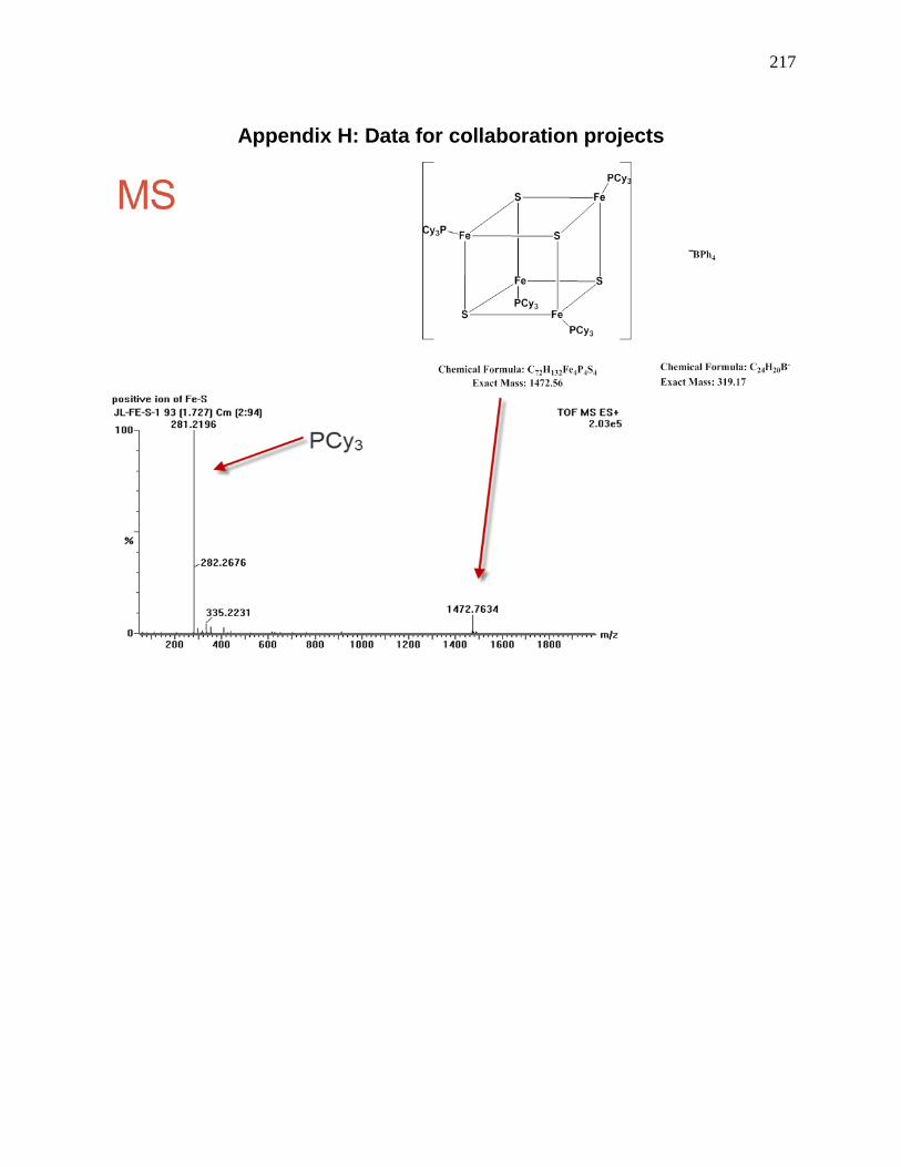
217
Appendix H: Data for collaboration projects
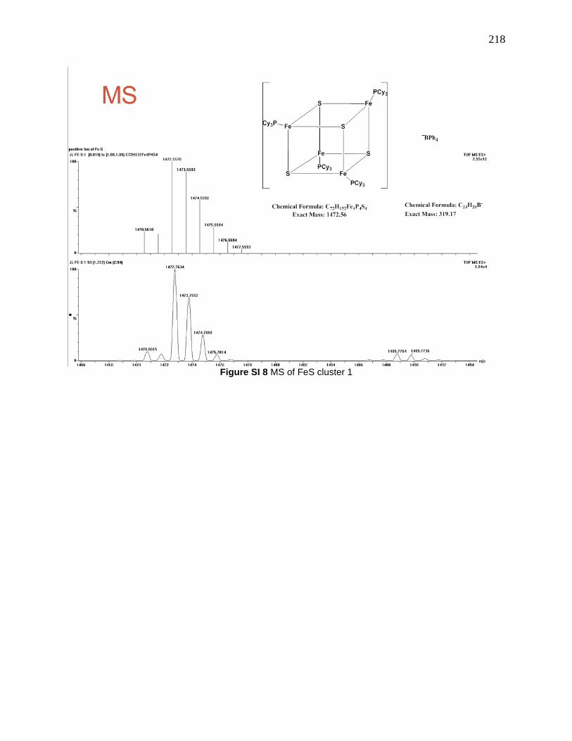
218
Figure SI 8 MS of FeS cluster 1

219
Figure SI 9 MS/MS of FeS cluster 1
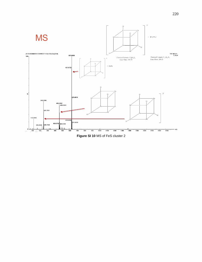
220
Figure SI 10 MS of FeS cluster 2
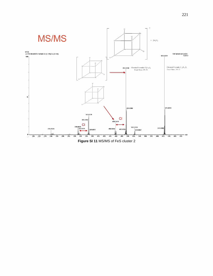
221
Figure SI 11 MS/MS of FeS cluster 2

222
Figure SI 12 MS of FeS cluster 3
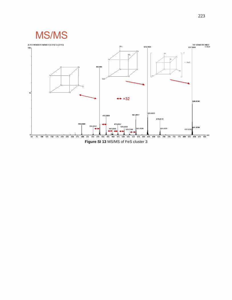
223
Figure SI 13 MS/MS of FeS cluster 3

224
Figure SI 14 Initial MS of catalyst only for Zn polymerization project
Table 8 Assignment of peaks in the spectrum
C23H25NOP 362.1
7
catalyst loss one
arm
C27H34NOP2 450.2
1
catalyst loss N-Bn
C27H34NO2P2 466.2
1
not very sure of
the structure,
C34H41N2OP2 555.2
7
this is the ligand
drop from catalyst
C38H47N2O4P2
Zn
721.2
3
this is the catalyst
charge is on Zn
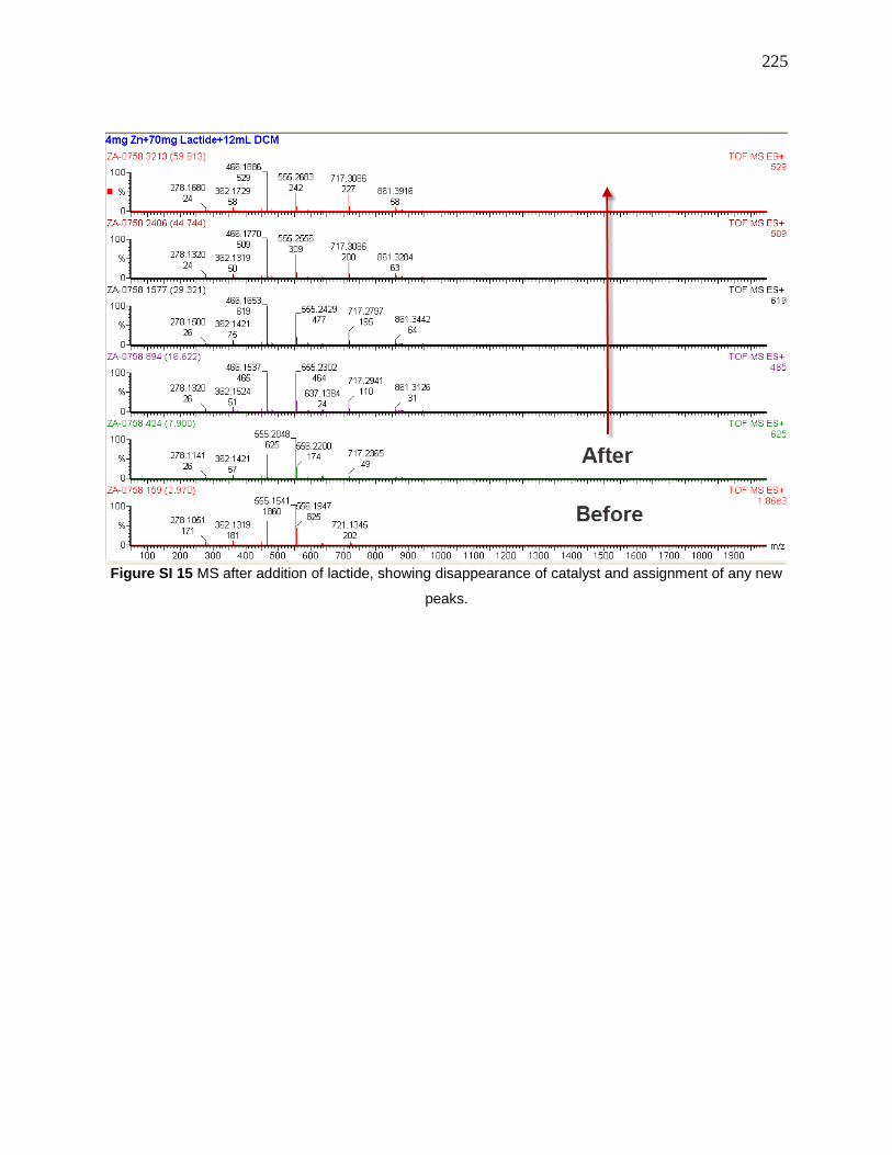
225
Figure SI 15 MS after addition of lactide, showing disappearance of catalyst and assignment of any new
peaks.
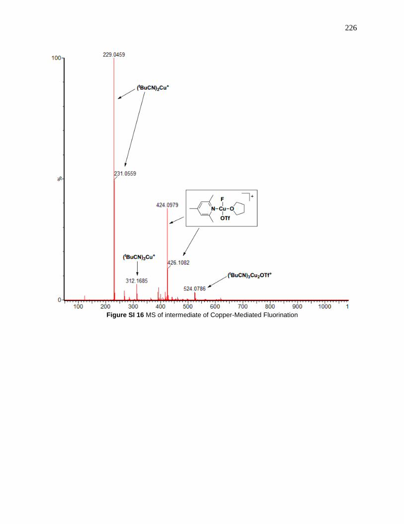
226
Figure SI 16 MS of intermediate of Copper-Mediated Fluorination
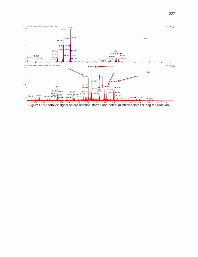
227
Figure SI 17 catalyst signal before reaction started and potential intermediates during the reaction.

228
Figure SI 18 Potential activated version of Pd(η
3-1-PhC3H4)(η
5-C5H5).