mechanisms of sedimentation inferred from …

MECHANISMS OF SEDIMENTATION INFERRED FROM QUANTITATIVE

CHARACTERISTICS OF HEAVY AND LIGHT MINERALS SORTING AND

ABUNDANCE

A Dissertation

by

KANNIPA MOTANATED

Submitted to the Office of Graduate and Professional Studies of

Texas A&M University

in partial fulfillment of the requirements for the degree of

DOCTOR OF PHILOSOPHY

Chair of Committee, Michael M. Tice

Committee Members, Thomas D. Olszewski

David Sparks

Scott A. Socolofsky

Head of Department, John R. Giardino

August 2014

Major Subject: Geology

Copyright 2014 Kannipa Motanated

ii

ABSTRACT

Hydraulic behaviors of particles with contrasting sizes and densities and flow

structure of hyperconcentrated suspensions were empirically studied in a thin vessel by

using particle-image-velocimetry techniques. Particle volumetric concentration, , of

the suspensions were mainly affected by the majority particle species, silica ballotini.

The minority population was aluminum ballotini (hydraulically fine). At high ,

aluminum particles were less retarded and settled as if they were hydraulically coarser.

This was because particles moved in a cluster-like motion. Terminal settling velocities of

both particles converged at 25%, and particle sorting was diminished.

Spatial and size distributions of mineral grains with contrasting densities in

massive sandstones of turbidites from the Middle Permian Brushy Canyon Formation

were used to estimate suspended sediment concentrations and interpret hydraulic

evolution of the turbidity currents. Semi-quantitative elemental distributions were

estimated by x-ray fluorescence analytical microscopy, µXRF. Within the structureless

sandstone, zircon grains (hydraulically fine) fined upward while feldspar grain

(hydraulically coarse) sizes did not change. Both grains had hydraulically equivalent

settling velocities in overlying siltstone layers. These suggest that these sandstone

divisions were deposited from hyperconcentrated suspensions where particle segregation

was diminished and hydraulically fine grains were entrained with hydraulically coarse

particles. While structureless sandstones were deposited, increased through distance

iii

and time because hydraulically fine particles were fining upward. This evolution likely

be resulted from volumetric collapse of the turbidity currents.

Geochemical concentrations and properties of Zr- and Ti-rich particles were used

to qualitatively estimate erosional event sizes of hemipelagic thinly laminated siltstone.

Zircon and rutilated quartz particle sizes, Zr/Ti fluorescence ratio, and lamination

thickness were determined by µXRF. Zircon grains were finer than rutilated quartz

grains. Their grain sizes were systematically correlated but neither was correlated with

Zr/Ti ratio. Instead, Zr/Ti ratio covaried with lamination thickness. Since zircon grains

are smaller but heavier than rutilated quartz grains, zircon has lower susceptibility to

erosion, particularly by wind. Thus, fluctuations of Zr/Ti fluorescence ratio in Brushy

canyon Formation siltstones most likely result from variations in the intensity of

erosional events at the particle source or sources, with high Zr/Ti ratios reflecting

periods of intense erosion.

iv

ACKNOWLEDGEMENTS

I would like to thank my committee chair, Dr. Michael M. Tice, for his advice,

constructive comments, and support. I would also like to thank my committee members,

Dr. Thomas D. Olszewski, Dr. David Sparks, and Dr. Scott A. Socolofsky, for their

guidance and insightful knowledge throughout the course of this research. Thanks to

Amanda D. Kallus and Spencer B. Gunderson for their helps in the field. Thanks also go

to Jian Gong for his help on setting up the experiments. I would like to thank Prof. Dr.

Peter Vennemann for his help on JPIV software. I also want to extend my gratitude to

the National Parks Department for their cooperation.

Lastly, I would like to thank friends, colleagues, and the department faculty and

staff for making my time at Texas A&M University a great experience.

v

TABLE OF CONTENTS

Page

ABSTRACT .......................................................................................................................ii

ACKNOWLEDGEMENTS .............................................................................................. iv

TABLE OF CONTENTS ................................................................................................... v

LIST OF FIGURES ..........................................................................................................vii

LIST OF TABLES ............................................................................................................ xi

CHAPTER I INTRODUCTION ........................................................................................ 1

1.1 Organization ............................................................................................................. 3

1.2 Objective .................................................................................................................. 3

CHAPTER II EXPERIMENTAL CHARACTERIZATION OF HEAVY MINERAL

SORTING FROM DENSE SUSPENSIONS OF LIGHT MINERAL GRAINS ............... 5

2.1 Introduction .............................................................................................................. 5

2.2 Background .............................................................................................................. 6 2.3 Methods of Study ..................................................................................................... 8

2.3.1 Experimental Setup ........................................................................................... 8

2.3.2 Particle-Imaging Technique ............................................................................ 10 2.4 Results .................................................................................................................... 12

2.4.1 Terminal Settling Velocities ............................................................................ 12

2.4.2 Settling Flow Structures .................................................................................. 13 2.5 Analysis and Discussion ........................................................................................ 26

2.5.1 Terminal Settling Velocities ............................................................................ 26 2.5.2 Settling Flow Structures .................................................................................. 28

2.6 Conclusions ............................................................................................................ 30

CHAPTER III HYDRAULIC EVOLUTION OF TURBIDITY CURRENTS FROM

HIGH TO LOW DENSITIES .......................................................................................... 32

3.1 Introduction and Background ................................................................................. 32 3.2 Methods of Study ................................................................................................... 34

3.3 Results .................................................................................................................... 35 3.3.1 Zircon Abundance Trends ............................................................................... 35

vi

3.3.2 Grain Sorting and Grading .............................................................................. 36 3.4 Analysis and Discussion ........................................................................................ 41

CHAPTER IV SILTSTONE ELEMENTAL COMPOSITIONS: A PROXY FOR

EROSIONAL EVENT SIZES, BRUSHY CANYON FORMATION, WEST TEXAS

AND SOUTH NEW MEXICO ........................................................................................ 44

4.1 Introduction and Background ................................................................................. 44 4.2 Methods of Study ................................................................................................... 48 4.3 Results .................................................................................................................... 50

4.3.1 Zircon and Rutilated Quartz Concentrations and Distributions ...................... 50

4.3.2 Lamination Thickness ..................................................................................... 54

4.4 Analysis and Discussion ........................................................................................ 58

4.4.1 Sources of Zr/Ti Ratio Variation ..................................................................... 58 4.5 Conclusions ............................................................................................................ 59

REFERENCES ................................................................................................................. 60

vii

LIST OF FIGURES

Page

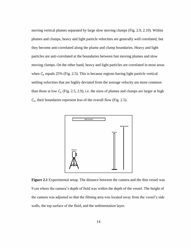
Figure 2.1 Experimental setup. The distance between the camera and the thin vessel

was 9 cm where the camera’s depth of field was within the depth of the

vessel. The height of the camera was adjusted so that the filming area was

located away from the vessel’s side walls, the top surface of the fluid, and

the sedimentation layer. .................................................................................... 14

Figure 2.2 Example image pre-processing steps by ImageJ. Each image is 19 mm x

12 mm. A) An image at initial time, , extracted from a video file at =

25%. B) An image at time = s. C) and D) Light particle

images derived from A) and B), respectively. E) and F) Heavy particle

images derived from A) and B), respectively. .................................................. 15

Figure 2.3 Example vector image processing steps by JPIV. A) A vector map of light

particles processed from Fig. 2.2 C) and D). B) A vector map of light

particles from A) subtracted by the average velocity of light particles,

. Areas where light particles move relatively slower than the

average velocity have low values, vice versa. C) A vector map of heavy

particles processed from Fig. 2.2 E) and F). D) A vector map of heavy

particles from C) subtracted by the average velocity of light particles,

. ........................................................................................................... 16

Figure 2.4 Example vector and vector contour maps processed by MATLAB. Each

image is 18 mm x 11 mm. A) A velocity vector map of light particles from

Fig. 2.3 B) plotted by MATLAB. B) The velocity vector map from A)

overlaid by contour lines of normalized vertical velocity of light particles,

| |. Areas where particles moved relatively slower than

the average velocity have negative values, vice versa. C) A velocity vector

map of heavy particles from Fig. 2.3 D) plotted by MATLAB. D) The

velocity vector map from C) overlaid by contour lines of normalized

vertical velocity of heavy particles, | |. ........................... 17

Figure 2.5 A) Example correlation between vertical velocity of light and heavy

particles from Fig. 2.4 A) and C) is presented by the product of

| | and | |. Areas where both light and heavy

particles moved relatively faster or slower than the average vertical velocity

of the light particles, , have positive values, correlated. Areas where one

particle species moved relative slower than and the other particle

viii

species moved relatively faster than result in negative values, anti-

correlated. B) Fig. 2.4 A) overlaid by Fig. 2.5 A). All vectors are grouped

and colored according to the standard deviation, , of the normalized

velocity vector data into five groups (1) red: , (2) orange:

, (3) green: , (4) light blue:

, and (5) dark blue . .................................... 18

Figure 2.6 Example particle velocity (cm s-1

) with respect to time (s) at = 20%.

Velocity fluctuation decayed at time > 100 s. .................................................. 19

Figure 2.7 Terminal settling velocities of glass and aluminum beads at different

suspended sediment concentrations. Error bars are ± 1 standard error of the

mean for 3-5 experiments at > 0 or 13-31 experiments at = 0%. The

lower limit of the bulk rheology model is at = 5%. ( = glass beads in

bimodal suspension; = aluminum beads in bimodal suspension; =

Richardson-Zaki settling velocity for glass beads; = Richardson-Zaki

settling velocity for aluminum beads; . .

= bulk rheology model for glass

beads; --- = bulk rheology model for aluminum beads; = glass beads in

monodisperse suspension). ............................................................................... 20

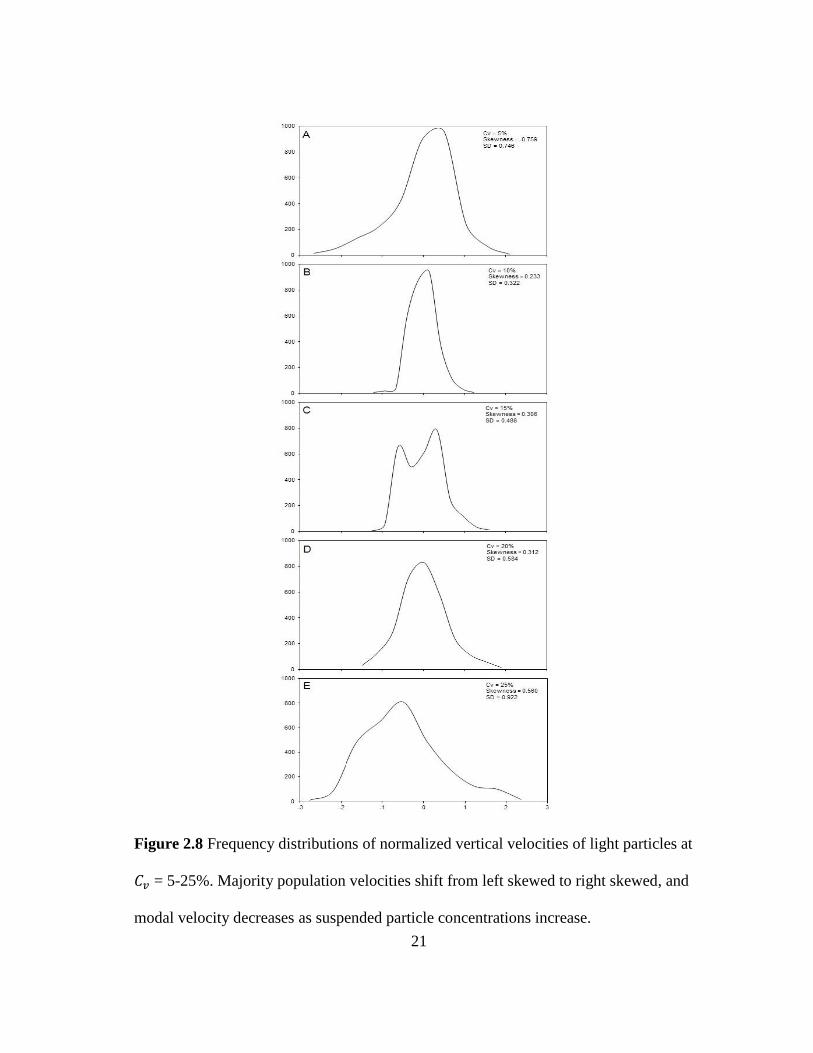
Figure 2.8 Frequency distributions of normalized vertical velocities of light particles

at = 5-25%. Majority population velocities shift from left skewed to right

skewed, and modal velocity decreases as suspended particle concentrations

increase. ............................................................................................................ 21

Figure 2.9 Normalized velocity vector map overlaid by contour map of light-heavy

vertical velocity correlation at = 5%. Vertical velocity vector component

of light particle species, , are normalized with respect to the average

vertical velocity component of the light particle, . All vectors are

grouped and colored according to the standard deviation, , of the

normalized velocity vector data into five groups (1) , (2)

, (3) , (4) ,

and (5) . ..................................................................................... 22


vertical velocity correlation at = 15%. Vertical velocity vector

component of light particle species, , are normalized with respect to the

average vertical velocity component of the light particle, . All vectors are



, (3) , (4) ,

and (5) . Example of elutriation effect can be observed at the

ix

horizontal distance of 14-15 mm. In these areas, heavy and light particles

are anti-correlated, and downward moving light particles caused relative

slower, than , moving heavy particles. ........................................................ 23


vertical velocity correlation at = 20%. Vertical velocity vector

component of light particle species, , are normalized with respect to the

average vertical velocity component of the light particle, . All vectors are



, (3) , (4) ,

and (5) . ..................................................................................... 24

Figure 2.12 Ratio of total area with negative light-heavy velocity correlation to

totalarea with positive light-heavy velocity correlation with respect to

particle volumetric concentration, . Decreasing ratio reflects organization

of the settling flow into increasingly large clumps. .......................................... 25

Figure 2.13 Average light-heavy correlation increases as increases above 10%. ....... 25

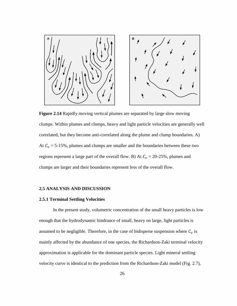
Figure 2.14 Rapidly moving vertical plumes are separated by large slow moving

clumps. Within plumes and clumps, heavy and light particle velocities are

generally well correlated, but they become anti-correlated along the plume

and clump boundaries. A) At = 5-15%, plumes and clumps are smaller

and the boundaries between these two regions represent a large part of the

overall flow. B) At = 20-25%, plumes and clumps are larger and their

boundaries represent less of the overall flow. .................................................. 26

Figure 3.1 A) Structureless sandstone sample bounded above by 1-cm-thick soft-

sediment-deformed black siltstone and below by 1-cm-thick thinly

laminated siltstones. B) and C) Normalized K fluorescence and Zr

fluorescence profiles, respectively, to represent feldspar and zircon

distributions with respect to height above the lower siltstone. Within the

structureless sandstone section, K fluorescence remains relatively constant

while that of Zr decreases upward.................................................................... 37

Figure 3.2 Normal probability plots of grain sizes (phi) and settling velocities at

infinite dilution for feldspar () and zircon () grains. A) and B) Normal

probability plots of light and heavy grain diameters (phi) of the massive

sandstone and the overlying black siltstone, respectively. C) and D) Stokes

setting velocities (cm s-1

) at infinite dilution of light and heavy particles in

the massive sandstone and the overlying black siltstone, respectively. Heavy

and light populations in siltstone are hydraulically equivalent while those of

sandstones are not, referred to panels D and C, respectively. .......................... 38

x

Figure 4.1 A prominent structureless sandstone bed exposed on Salt Flat Bench

(vertically exaggerated outcrop photo to show different deposits). The

measured sections came from thinly laminated siltstone outcrops (Gray

Siltstone) overlying this late-stage channel filling structureless sandstone.

The sampling location’s GPS coordinates: N 31.871, W 104.858. Modified

from Gunderson (2011).................................................................................... 49

Figure 4.2 Normal probability plots of rutilated quartz grain sizes from small scans

show that these grains are normally distributed (R2 = 0.988; p = 10

-33). .......... 51

Figure 4.3 Rutilated quartz grain size (phi) with respect to zircon grain size (phi) from

each 10 µm resolution scanning location is shown in . A line of 1:1 grain

size ratio is displayed in . Linear regression line (- - -) has a slope of 1.098

± 0.316 (95% confidence) and p-value of 10-8

. ................................................ 52

Figure 4.4 Zr/Ti fluorescence ratio with respect to Ti-rich mineral grain size (phi) (R2

= 0.016; p for the regressed slope 0.489).......................................................... 53

Figure 4.5 Zr/Ti fluorescence ratio with respect to Zr-rich mineral grain size (phi) (R2

= 0.014; p for the regressed slope = 0.472). ..................................................... 53

Figure 4.6 Fe-rich bands occur along black laminae. A) MBC 1-5 rock sample. B) Fe-

fluorescence of MBC 1-5 rock sample. ............................................................ 56

Figure 4.7 Correlation plots of lamination thickness and Zr/Ti fluorescence ratio. All

samples have positive correlation. .................................................................... 57

xi

LIST OF TABLES

Page

Table 3.1 Paired sample t-tests of Zr- and K-rich grain sizes. ......................................... 39

Table 3.2 Two-way repeated measures analysis of variance of grain size for zircon

and feldspar grain sizes. .................................................................................... 40

Table 4.1 Linear regression and correlation analysis between lamination thickness

and Zr/Ti ratio. Lamination thickness and Zr/Ti ratio are positively

correlated in every sample................................................................................ 55

1

CHAPTER I

INTRODUCTION

Beaubouef et al. (1999) estimated that at least 90% of the Brushy Canyon

Formation, Delaware Basin, west Texas and southeast New Mexico was deposited as

turbidites and the rest as debrites and hemipalegites. The structureless sandstones of the

Brushy Canyon Formation have been extensively researched and interpreted as fine-

grained sandstones deposited by rapid fallout from turbid suspensions (Beaubouef et al.,

1999). In the Upper Brushy Canyon Formation, structureless sandstones were deposited

as channel infill during a relatively low sea level. Since light and heavy minerals are

hydraulically sorted in sands, analysis of sediment sorting and distribution is commonly

used for interpreting flow properties, mechanisms of deposition and transportation, and

relative transport distance of sediments (e.g., Allen, 1991; Bowen et al., 1984; Komar,

1985; Middleton, 1976; Rubey, 1933; Slingerland and Smith, 1986; Slingerland, 1977;

Steidtmann, 1982; Van Tassell, 1981; Visher, 1969).

Sedimentation processes are commonly exploited in heavy mineral separation

processes in the chemical and mining industries. Theoretical and empirical studies of

mechanisms of sedimentation and liquid-solid fluidization have been extensively

researched and they are applicable to sedimentological problems, as well. Middleton and

Southard (1984) explained the differences in mechanisms of sediment movement in

infinitely dilute and concentrated suspensions. When a particle settled through a still

viscous fluid, it accelerated until the upward fluid drag force was equal to the

2

gravitational force. Then, the particle would fall at a constant velocity called the terminal

settling velocity. Russel et al. (1984) quantitatively studied fluid-solid and solid-solid

interactions in colloidal suspensions. The study revealed that in finite volumetric

sediment concentrations, terminal settling velocities were different and much more

complex from those in infinitely dilute suspensions. Interactions between particles had a

great influence on sedimentation. These particle interactions should be reflected in the

spatial distribution of suspension. Thus, the spatial distribution of suspension during

settling is critical for evaluating the relationship between sedimentation and particle

volumetric concentration of suspensions. Vector maps of particle movements are,

therefore, essential for understanding the sedimentation processes in highly concentrated

suspensions.

The central theme of this dissertation is the use of heavy minerals as probes of

depositional processes. Empirical study on settling velocities of particles with

contrasting sizes and densities in hyperconcentrated suspension leads to an insightful

understanding of flow structure and particle’s hydraulic behaviors. The results from this

chapter can be used to interpret flow evolution of turbidites. The last chapter uses the

relationship between particle sizes and abundances as qualitative proxies for the intensity

of erosional events of hemipelagic thinly laminated siltstone in the Brushy Canyon

Formation of west Texas and south New Mexico.

3

1.1 ORGANIZATION

This dissertation is organized into three main chapters. Chapter II presents an

experimental study of heavy mineral sorting in dense suspensions of light mineral grains,

where heavy particles are the minority and the light particles are the majority

populations. Chapter III analyzes hydraulic evolution of turbidity currents from high to

low densities based on heavy and light mineral sorting and distribution. Chapter IV

presents estimation of erosional event sizes of thinly laminated siltstone by using

geochemical properties as proxies.

1.2 OBJECTIVE

The objectives of the second dissertation chapter are to use grain settling

experiments conducted in a thin vessel and particle-image-velocimetry (PIV) techniques

(1) to study spatial distribution and sorting of light and heavy minerals at various

volumetric concentrations and (2) to analyze inter-particle and particle-fluid interactions

during hindered settling as a function of volumetric concentration.

The objectives of the third chapter are (1) to detect and characterize heavy and

light mineral (Zr- and K-bearing particles, respectively) sorting and distribution within

structureless sandstones from the Brushy Canyon Formation, Delaware Basin, southern

New Mexico and (2) to use grain size distributions of mineral grains with contrasting

densities and the results from Chapter II to quantitatively describe the turbidity flow’s

evolution.

4

The objectives of the fourth chapter are (1) to detect and characterize sorting and

distribution of heavy, Zr-bearing grains, and light, Ti-bearing grains, with in the thinly

laminated siltstones of the Brushy Canyon Formation, Delaware Basin, southern New

Mexico and (2) to use geochemical properties as proxies to qualitatively analyze sources

of Zr/Ti fluorescence ratio variation.

5

CHAPTER II

EXPERIMENTAL CHARACTERIZATION OF HEAVY MINERAL SORTING

FROM DENSE SUSPENSIONS OF LIGHT MINERAL GRAINS

2.1 INTRODUCTION

Particles’ transport and deposition processes depend on their size, shape, density,

and grain support mechanisms. Gross changes in sediment concentration can produce

diagnostic transitions between different types of deposits (e.g., Amy et al., 2006; Felix,

2002). Richardson and Meikle (1961) experimentally studied sedimentation and settling

velocity of mixtures of equal volumes of heavy glass ballotini and light polystyrene.

Amy et al. (2006) experimentally investigated sand-mud suspension settling behavior.

Their research results concluded that particle segregation depended on particle

volumetric concentration, . However, heavy mineral grains are commonly

hydraulically finer than light mineral grains in the same sediment source. The existing

literature is not clear on how mixtures of these grains will settle. This research

empirically studies flow structures and hydraulic behaviors of heavy particles that are

hydraulically finer than light particles, at various . The particle volumetric

concentration of small heavy particles is low enough that they are treated like the

minority particles, similar to what can be found in nature.

6

2.2 BACKGROUND

For particles in uniform suspensions with > 1%, the force resisting settling

results from the velocity gradient due to the upward movement of fluid displaced by the

downward movement of particles (e.g., Davis et al., 1988; Nicolai et al., 1995;

Richardson and Zaki, 1954). The settling velocity of a particle in concentrated

suspension is lower than its Stokes velocity because of viscosity enhancement by the

surrounding particles and fluid backflow generated by the motion of nearby particles; it

is well-described by Equation 2.1 (Richardson and Zaki, 1954):

( ) . (2.1)

Here, is the Richardson-Zaki particle settling velocity at volumetric concentration

. is the Stokes velocity and is a function of particle Reynolds number. For small

particle Reynolds number, 5 (Nicolai et al., 1995).

Alternatively, concentrated suspensions can behave as Bingham plastics with

effective yield strengths and dynamic viscosities that are functions of (Julien, 1998;

Julien and Lan, 1991). In this case, yield strength and dynamic viscosity of the fluid are

affected by suspended sediments due to cohesion between particles, internal friction

between fluid and sediment particles, turbulence, and particle-particle collisions.

Consequently, hyperconcentrated mixtures of homogeneous fine grains and fluid possess

an apparent yield strength, (Equation 2.2), beyond which the rate of deformation,

7

⁄ , is linearly proportional to the excess shear stress. Yield strength, , for a

mixture ( > 5%) and dynamic viscosity of a mixture, , and are given by

( ) ( ) (2.2)

and

( ( )) . (2.3)

Here, is the dynamic viscosity of the fluid at = 0. This mixture has an average

density of ( ), where is the density of the fluid and is the

density of the particle. The settling velocity of a particle in a Bingham plastic fluid, ,

can be expressed as a function of particle diameter, , and drag coefficient, ,

√

.

(2.4)

can be written as a function of particle Reynolds, , and Hedstrom number

This can be expressed as

. (2.5)

8

Julien’s particle settling velocity, , which is obtained from Equations (2.4) and (2.5), is

expressed as

{(

( )

)

} (2.6)

In the Richardson-Zaki model, particles that are hydraulically fine will always

settle slower than hydraulically coarse particles. As a result, particles that are

hydraulically different will not sort and deposit together. In Julien’s model, particles that

are hydraulically fine can have equal or greater settling velocities than hydraulically

coarse particles in fluid that is hyperconcentrated with fine grains. Particles with

contrasting sizes and densities could thus be sorted and deposited together. Heavy

particles are commonly smaller and have fewer abundance. This research is focused on

an empirical study of the hydraulic behaviors of particles with contrasting sizes and

densities at particle volumetric concentrations ranging from 5% to 25%. The results from

this study could be used to analyze deposits of concentrated suspensions such as high

density turbidity currents.

2.3 METHODS OF STUDY

2.3.1 Experimental Setup

This research project modifies the experimental approach of Segre et al. (2001)

to study the sorting mechanisms of bimodal suspensions—particles with contrasting

9

sizes and densities—at various particle volume fractions, . In this research,

sedimentation of solid particles at different volume fractions of particles in a fluid was

experimentally studied by dispersing spherical glass and aluminum particles within a

glycerol-water mixture in a clear rectangular vessel (Fig. 2.1). The calculated fluid

dynamic viscosity, , and the measured density, , of glycerol-water mixture

were 0.016 ± 0.002 Pa s (standard error from 44 measurements) and 1177 ± 3.31 kg m-3

(standard error from 4 measurements), respectively, at room temperature of 24 ± 2 oC.

The vessel was 6 cm wide, 0.5 cm thick, and 30 cm high (Fig. 2.1). Two spherical

particle species of lighter, larger silica and denser, smaller aluminum beads were used in

this research. Silica glass beads had diameters of 90-106 µm and a density of 2.45-2.50 g

cm-3

. Aluminum beads were originally manufactured in metallic white color, and had a

diameter of 70 µm and density of 3.75 g cm-3

. They were then dyed black with India ink

that consequently increased the aluminum beads’ diameters and decreased their

densities. Black aluminum beads had measured diameters of 73 ± 3 µm (standard errors

from 10 measurements) and a density of 2.78 ± 0.02 g cm-3

(calculated from their

settling velocities at infinitely dilute suspension; standard error from 31 measurements).

Silica and aluminum beads are hereafter referred to as light and heavy particles based on

their relative densities. Particle settling velocities at infinitely dilute suspension was

determined from dropping each particle grain into the glycerol-water mixture and

recorded its traveling distance and time. In an infinitely dilute suspension, silica and

aluminum particles had settling velocities of 0.57 ± 0.03 and 0.27 ± 0.03 mm s-1

,

respectively (standard errors derived from 13 and 31 measurements on silica and

10

aluminum particle species, respectively). Both particles’ Reynolds numbers were

approximately 10-4

. Settling experiments were divided into two parts. First,

monodisperse suspension of silica beads at particle volumetric concentrations, , of

5%, 10%, 15%, and 20% in order to test the validity of the experimental setup. Second,

binary mixtures of silica and aluminum beads had of 5%, 10%, 15%, 20%, and 25%.

In every bidisperse suspension, the concentration of aluminum particle in the total

concentration of solids was less than 1%. Therefore, the total particle volumetric

concentration of each bidisperse suspension was mainly controlled by the amount of

silica beads. Consequently, the hydraulic properties of small, dense aluminum beads in

concentrated suspension were dominated by the presence of the more abundant silica

beads.

Since the experiments were carried out in a confining container, the container

walls could potentially retard settling (Chhabra et al., 2003; Di Felice, 1996; Machac and

Lecjaks, 1995). In these experiments, the wall factor, , was dependent on the ratio of

particle diameter to effective container diameter because particle Reynolds number was

very low (Chhabra et al., 2003). of silica glass and aluminum particles, calculated by

using experimental results from Machac and Lecjaks (1995), equaled 0.980-0.983 and

0.985-0.986, respectively. Therefore, the effect of confining walls on both particle

species was negligible.

2.3.2 Particle-Imaging Technique

Particles were soaked in the glycerol-water mixture prior to the settling

experiment in order to prevent air bubbles and particle cohesion. The vessel was

11

vigorously agitated in order to thoroughly mix the beads with the surrounding fluid into

a homogeneous mixture. Images of particle movements at a frequency of 60 frames per

second were recorded by a charge-coupled device (CCD) using a depth of field of 0.5-

0.7 cm. ImageJ software was used for image processing procedures including

digitization, stacking, and background color correction of still-images of particle

positions (Fig. 2.2). Velocity vector maps representing magnitude and vector of grain

movement were calculated by using standard particle-image-velocimetry (PIV)

techniques (Fig. 2.3). Since the aluminum beads were opaque and dyed with black India

ink while the glass beads were white, they were visibly distinguishable (Fig. 2.2).

MATLAB was used to calculate and generate normalized velocity vector, velocity

contour, and particle correlation maps from particle velocity vectors derived by JPIV

(Fig. 2.4, 2.5).

Vector maps of grain movements were generated from image frames at a time

interval of 5/60 or 0.083 seconds via iterative JPIV software (Fig. 2.2, 2.3). The software

computed velocity vectors based on the cross-correlation of the intensity distributions

over the assigned areas within the flow. In this experiment, each study area was 18 mm x

11 mm or 19 mm x 12 mm. The interrogation window and search domain were set to be

32 pixels x 32 pixels (0.69 mm x 0.69 mm) and 8 pixels x 8 pixels (0.17 mm x 0.17

mm), respectively. Horizontal and vertical velocity vector components were computed

(horizontal and vertical vector spacing of 0.25 mm x 0.25 mm) at this step. Terminal

settling velocities were determined when the vertical velocity fluctuation of the light

particle had decayed (Fig. 2.6). Flow structures were visualized through magnitude and

12

direction of velocity vectors and correlation between the directions of the particles’

movement. The main objective of the experiments was to analyze the hindered settling

effects on heavy minerals as a function of volumetric concentration, . Thus, particle-

particle and fluid-particle interactions were the main focuses in this study.

2.4 RESULTS

2.4.1 Terminal Settling Velocities

Terminal settling velocity of glass beads from both monodisperse and bidisperse

suspensions are compared with the hindered settling model of Richardson and Zaki

(1954) in order to test the validity of this experiment (Fig. 2.7). Terminal settling

velocities of both glass and aluminum beads at of 5-25% are compared against the

existing formulas proposed by Richardson and Zaki (1954) and Julien (1998). Terminal

settling velocity of light particles in monodisperse and bidisperse suspensions are in

good agreement (within ± 1 standard error) with the predicted values from Richardson

and Zaki (1954). However, the terminal settling velocity of heavy particles (the minority

particle species) calculated from Richardson-Zaki is lower than the experimental data at

5%.

The terminal settling velocities of silica beads (the majority particle) are well

described by Richardson-Zaki (1954) with = 5.8 ± 0.9 (standard error for the slope of a

log-log regression of on ). The terminal settling velocities of aluminum beads

(the minority particle) has = 4.1 ± 0.5 (standard error for the slope of a log-log

regression of on ).

13

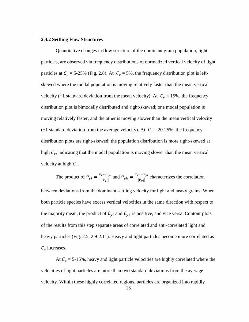
2.4.2 Settling Flow Structures

Quantitative changes in flow structure of the dominant grain population, light

particles, are observed via frequency distributions of normalized vertical velocity of light

particles at = 5-25% (Fig. 2.8). At = 5%, the frequency distribution plot is left-

skewed where the modal population is moving relatively faster than the mean vertical

velocity (+1 standard deviation from the mean velocity). At = 15%, the frequency

distribution plot is bimodally distributed and right-skewed; one modal population is

moving relatively faster, and the other is moving slower than the mean vertical velocity

(±1 standard deviation from the average velocity). At = 20-25%, the frequency

distribution plots are right-skewed; the population distribution is more right-skewed at

high , indicating that the modal population is moving slower than the mean vertical

velocity at high .

The product of

| | and

| | characterizes the correlation

between deviations from the dominant settling velocity for light and heavy grains. When

both particle species have excess vertical velocities in the same direction with respect to

the majority mean, the product of and is positive, and vice versa. Contour plots

of the results from this step separate areas of correlated and anti-correlated light and

heavy particles (Fig. 2.5, 2.9-2.11). Heavy and light particles become more correlated as

increases.

At = 5-15%, heavy and light particle velocities are highly correlated where the

velocities of light particles are more than two standard deviations from the average

velocity. Within these highly correlated regions, particles are organized into rapidly

14

moving vertical plumes separated by large slow moving clumps (Fig. 2.9, 2.10). Within

plumes and clumps, heavy and light particle velocities are generally well correlated, but

they become anti-correlated along the plume and clump boundaries. Heavy and light

particles are anti-correlated at the boundaries between fast moving plumes and slow

moving clumps. On the other hand, heavy and light particles are correlated in most areas

when equals 25% (Fig. 2.5). This is because regions having light particle vertical

settling velocities that are highly deviated from the average velocity are more common

than those at low (Fig. 2.5, 2.9), i.e. the sizes of plumes and clumps are larger at high

, their boundaries represent less of the overall flow (Fig. 2.5).

Figure 2.1 Experimental setup. The distance between the camera and the thin vessel was

9 cm where the camera’s depth of field was within the depth of the vessel. The height of

the camera was adjusted so that the filming area was located away from the vessel’s side

walls, the top surface of the fluid, and the sedimentation layer.

15

Figure 2.2 Example image pre-processing steps by ImageJ. Each image is 19 mm x 12

mm. A) An image at initial time, , extracted from a video file at = 25%. B) An

image at time = s. C) and D) Light particle images derived from A) and B),

respectively. E) and F) Heavy particle images derived from A) and B), respectively.

A B

C D

E F

16

Figure 2.3 Example vector image processing steps by JPIV. A) A vector map of light

particles processed from Fig. 2.2 C) and D). B) A vector map of light particles from A)

subtracted by the average velocity of light particles, . Areas where light particles

move relatively slower than the average velocity have low values, vice versa. C) A

vector map of heavy particles processed from Fig. 2.2 E) and F). D) A vector map of

heavy particles from C) subtracted by the average velocity of light particles, .

A B

C D

17

Figure 2.4 Example vector and vector contour maps processed by MATLAB. Each

image is 18 mm x 11 mm. A) A velocity vector map of light particles from Fig. 2.3 B)

plotted by MATLAB. B) The velocity vector map from A) overlaid by contour lines of

normalized vertical velocity of light particles, | |⁄ . Areas where

particles moved relatively slower than the average velocity have negative values, vice

versa. C) A velocity vector map of heavy particles from Fig. 2.3 D) plotted by

MATLAB. D) The velocity vector map from C) overlaid by contour lines of normalized

vertical velocity of heavy particles, | |⁄ .

A B

C D

18

Figure 2.5 A) Example correlation between vertical velocity of light and heavy particles

from Fig. 2.4 A) and C) is presented by the product of | |⁄ and

| |⁄ . Areas where both light and heavy particles moved relatively

faster or slower than the average vertical velocity of the light particles, , have positive

values, correlated. Areas where one particle species moved relative slower than and

the other particle species moved relatively faster than result in negative values, anti-

correlated. B) Fig. 2.4 A) overlaid by Fig. 2.5 A). All vectors are grouped and colored

according to the standard deviation, , of the normalized velocity vector data into five

groups (1) red: , (2) orange: , (3) green:

, (4) light blue: , and (5) dark blue .

A

B

19

Figure 2.6 Example particle velocity (cm s-1

) with respect to time (s) at = 20%.

Velocity fluctuation decayed at time > 100 s.

0

0.03

0.06

0.09

0.12

0.15

0 50 100 150 200 250

Part

icle

Velo

cit

y (

cm

/s)

Time (s)

20

Figure 2.7 Terminal settling velocities of glass and aluminum beads at different

suspended sediment concentrations. Error bars are ± 1 standard error of the mean for 3-5

experiments at > 0 or 13-31 experiments at = 0%. The lower limit of the bulk

rheology model is at = 5%. ( = glass beads in bimodal suspension; = aluminum

beads in bimodal suspension; = Richardson-Zaki settling velocity for glass beads;

= Richardson-Zaki settling velocity for aluminum beads; . .

= bulk rheology model for

glass beads; --- = bulk rheology model for aluminum beads; = glass beads in

monodisperse suspension).

0

0.01

0.02

0.03

0.04

0.05

0.06

0.07

0 0.05 0.1 0.15 0.2 0.25 0.3 0.35

Term

ina

l S

ett

lin

g V

elo

cit

y (

cm

/s)

Particle Volumetric Concentration (%)

21

Figure 2.8 Frequency distributions of normalized vertical velocities of light particles at

= 5-25%. Majority population velocities shift from left skewed to right skewed, and

modal velocity decreases as suspended particle concentrations increase.

22


vertical velocity correlation at = 5%. Vertical velocity vector component of light

particle species, , are normalized with respect to the average vertical velocity

component of the light particle, . All vectors are grouped and colored according to the

standard deviation, , of the normalized velocity vector data into five groups (1)

, (2) , (3) , (4)

, and (5) .

Horizontal Distance (mm)

Vert

ical D

ista

nc

e (

mm

)

23






, (2) , (3) , (4)

, and (5) . Example of elutriation effect can be observed at

the horizontal distance of 14-15 mm. In these areas, heavy and light particles are anti-

correlated, and downward moving light particles caused relative slower, than ,

moving heavy particles.


Vert

ical D

ista

nc

e (

mm

)

24






, (2) , (3) , (4)

, and (5) .


Vert

ical D

ista

nc

e (

mm

)

25

Figure 2.12 Ratio of total area with negative light-heavy velocity correlation to totalarea

with positive light-heavy velocity correlation with respect to particle volumetric

concentration, . Decreasing ratio reflects organization of the settling flow into

increasingly large clumps.

Figure 2.13 Average light-heavy correlation increases as increases above 10%.

0

0.1

0.2

0.3

0.4

0.5

0.6

0.7

0.8

0.9

0 5 10 15 20 25 30Neg

ati

ve/P

os

itiv

e s

cale

d v

ert

ical

velo

cit

y r

ati

o


0

1

1

2

2

3

0 5 10 15 20 25 30

Avera

ge

Vert

ical C

orr

ela

tio

n


26

Figure 2.14 Rapidly moving vertical plumes are separated by large slow moving

clumps. Within plumes and clumps, heavy and light particle velocities are generally well

correlated, but they become anti-correlated along the plume and clump boundaries. A)

At = 5-15%, plumes and clumps are smaller and the boundaries between these two

regions represent a large part of the overall flow. B) At = 20-25%, plumes and

clumps are larger and their boundaries represent less of the overall flow.

2.5 ANALYSIS AND DISCUSSION

2.5.1 Terminal Settling Velocities

In the present study, volumetric concentration of the small heavy particles is low

enough that the hydrodynamic hindrance of small, heavy on large, light particles is

assumed to be negligible. Therefore, in the case of bidisperse suspension where is

mainly affected by the abundance of one species, the Richardson-Zaki terminal velocity

approximation is applicable for the dominant particle species. Light mineral settling

velocity curve is identical to the prediction from the Richardson-Zaki model (Fig. 2.7),

A B

27

and = 5.82 ± 0.89 (95% confidence interval), which is similar to what has been

observed by other investigators, a Richardson-Zaki exponent of 5 (e.g., Nicolai et al.,

1995; Segre et al., 2001).

In contrast, heavy particle velocities in bidisperse suspensions are not well-fitted

by the prediction from Richardson-Zaki model. In particular, the heavy particle velocity

under infinite dilute conditions is low compared to the predicted value from the fitted

line (of heavy particle’s settling velocities in this study). To test the categorical effect

between heavy particle’s settling velocity at = 0 and at > 0 , a dummy variable

(qualitative explanatory variable), = 1 if = 0 and 0 otherwise, was added to the

regression. The regression coefficient of the dummy variable was significantly different

from 0 ( = 0.045). Also, this regression fit yielded an exponent of 4.84 ± 1.18 (95%

confidence interval) and an -squared value of 0.986. This evidence shows that heavy

grains behave coarser at even low and are not as hindered with increasing as the

Richardson-Zaki model predicts.

Settling velocities predicted from estimated bulk rheological properties (Julien

and Lan, 1991) are systematically lower than those observed in experiments. However,

the rheology model predicts that the settling velocities of light and heavy particles

converge at 20% < < 25%, and when is greater than 25%, the heavy particles settle

faster than the light particles. Convergence of velocities (within measurement error) is

observed in this study at 20% < < 25%. Observations do not extend beyond > 25%

because heavy particles were no longer distinguishable by the methods used here.

28

Therefore, where hydraulically fine settle faster than hydraulically coarse particles

were not observed in this study.

2.5.2 Settling Flow Structures

The ratio of anti-correlated to correlated light-heavy particles is dependent on

particle volumetric concentration, (Fig. 2.12). As particle volumetric concentration

increases, heavy and light particles become more correlated, and vice versa. The

normalized light-heavy correlation also increases when increases (Fig. 2.13). This is

because at low the mean distance between particles is high which results in a low

probability of particle-particle collision (Bagnold, 1962). Thus, particle-particle

interaction is not significant. As light particles form fast moving plumes and slow

moving clumps, heavy particles in both areas move relatively slower than light particles

because aluminum grains are hydraulically finer in an infinitely dilute suspension.

Additionally, when particle-particle interlocking is diminished, downward-moving

plumes of hydraulically coarse particles could cause relatively upward elutriation of

hydraulically fine particles (Davies, 1968) (Fig. 2.10). Therefore, at low , up to 40%

of light and heavy particles are anti-correlated, and terminal settling of heavy particles is

significantly slower than that of light particles.

Bagnold (1962) proposed that when 9%, the mean distance between

particles is equal or less than their diameter resulting in a significant probability of

particle collision. Thus, particle-particle interaction is dominant. In this study, at high ,

particles settle primarily in clumps and particle suspension microstructures are important

(Nicolai et al., 1995). Settling flow structures observed at 25% show that the majority

29

of light and heavy particles are correlated because they are interlocked (Fig. 2.5). The

difference in vertical velocity between the fast moving plumes and slow moving clumps

is not as high as those observed at low . Upward elutriations of hydraulically fine

particles are not observed which are similar to the empirical results of binary and tertiary

suspensions from Davies (1968). In that study, segregation of particles with equal

density but different sizes vanishes at concentrations higher than their critical

interlocking concentrations. Above these values, particle interlocking becomes dominant

and the upward elutriation of hydraulically fine particles is diminished. These limiting

values are dependent on particle size and shape and concentration of the total and each

species.

In this study, when particle volumetric concentration is high, both particle

species are interlocked and hydraulically fine aluminum particles are entrained with

hydraulically coarse silica particles. This behavior is similar to that observed by Hoyos

et al. (1994). In the suspension of noncolloidal bidisperse glass beads, large particles are

hindered while small particles are ‘dragged along’ due to the geometric limitations of

interlocking particles.

The settling velocity of the light particles (the majority population) is well-

predicted by the model from Richardson and Zaki (1954). However, this model

underestimates the terminal settling velocities of heavy particles (the minority

population) at high . This is because this model does not treat particles with

contrasting sizes and densities differently. As a result, settling velocities of heavy and

light particles never converge according to this model.

30

The rheology model from Julien (1998) underestimates the terminal settling

velocities of both particle species. However, this model predicts that the settling

velocities of heavy and light particles converge when 20% 25%, which is similar

to the results found in this research. Nevertheless, at 25%, the rheology model

predicts that heavy particles settle faster than light particles. If this is the case, in

hyperconcentrated suspension, heavy particles tend to accumulate at the bases of the

deposits and are overlaid by a mixture of heavy and light particles, assuming the overall

particle concentration of the flow is decreasing through time. Based on the results found

in this research, at high , the settling velocities of heavy and light particles converge

but are unlikely to crossover. This is because heavy particles are entrained by light

particles in clumps rather than settling between them.

2.6 CONCLUSIONS

This research demonstrated that at high particle volumetric concentration, 20%

25%, terminal settling velocities of hydraulically light and heavy particles

converge but are unlikely to crossover. At high , particle segregation was diminished

because particles settle in clumps and hydraulically fine particles (the minority species)

were trapped in locally dense clusters of hydraulically coarse particle (the majority

species). Within these clusters of fast moving plumes and slow moving clumps, both

particle species were moving coherently while they moved oppositely along the clusters’

boundaries. As increases, the difference in vertical velocity between the fast moving

plumes and slow moving clumps was not as high as those observed at low . Numbers

31

of clumps and jets were also decreasing and clumps’ sizes were increasing (Fig. 2.14).

Consequently, hydraulically different particles settled together at high , and particle

segregation was diminished. This result can be used to interpret volumetric

concentration and hydraulic evolution of turbidites where hydraulically different grains

coexist.

32

CHAPTER III

HYDRAULIC EVOLUTION OF TURBIDITY CURRENTS FROM HIGH TO LOW

DENSITIES

3.1 INTRODUCTION AND BACKGROUND

Transformations in sediment gravity flows as they move down slopes are critical

in determining the architectures of submarine depositional systems. These

transformations are driven by changing suspended sediment concentrations and

consequent changes in grain support mechanisms (e.g., Haughton et al., 2009; Mulder

and Alexander, 2001). As suspended sediment concentration increases from 1% to 9%,

the mean distance between suspended grains decreases from four particle diameters to

one particle diameter (Bagnold, 1962). As a result, particle-particle interactions become

more frequent and more important in maintaining particles in suspension. In low-

concentration turbidity currents, turbulence is the main particle support mechanism

(Haughton et al., 2009; Mulder and Alexander, 2001), and sediment support is

independent of particle concentration (Lowe, 1982). In high-concentration turbidity

currents, turbulence, grain-grain interactions, and fluid escape are the dominant support

mechanisms. Formation of bed forms is suppressed in such flow, resulting in deposits

without current structures such as Bouma Ta/ Lowe S3 divisions (Bouma, 1962; Lowe,

1982).

Because transport and deposition processes depend on grain support

mechanisms, gross changes in sediment concentration produce diagnostic transitions

33

between different types of deposits. In other words, turbidity currents are controlled by

suspended sediments (Felix, 2002) and their hydraulic properties are also recorded in

sediment deposits (e.g., Kneller and McCaffrey, 2003; Komar, 1985). However, changes

in concentration that do not result in changes in flow type are more difficult to diagnose

in deposits, making investigation of the mechanics of flow transformation challenging.

Naturally occurring heavy minerals can be used as tracer particles because

particles with contrasting sizes and densities settle differently under various volumetric

concentrations (Chap. 2). Since particles are hydraulically sorted according to their

transportability, which is a function of size, shape, and density, settling behavior of

bimodal suspensions has been a subject of continued interest (e.g., Amy et al., 2006;

Berthault, 1988; Steidtmann, 1982). Experimental investigation of settling behavior of

sand-mud suspension found five distinct deposits ranging from particle size segregation

to no size segregation (Amy et al., 2006). Each deposit is associated with different

settling regimes that result from changes in sediment concentration. A similar study of

bimodal mixtures between relatively dense ballotini and light polystyrene (equal Stokes

velocities and volumes) found that at particle volumetric concentration, , higher than

15%, light particles remained in suspension until heavy particles had completely settled.

At below 8%, there was no sediment segregation, both particles settled together

(Richardson and Meikle, 1961). However, a more universal threshold concentration

boundary is not clearly defined due to the complexity of factors such as particle sizes,

densities, and distributions (e.g., Mulder and Alexander, 2001).

34

This study uses zircon and feldspar grains as test particles to investigate changing

suspended sediment concentrations during deposition of Ta divisions of turbidites from

the Middle Permian Brushy Canyon Formation, Eddy County, southwest New Mexico.

More than 90% of the sandstones of the Brushy Canyon Formation were deposited as

turbidites (Beaubouef et al., 1999). Suspension deposits such as structureless beds,

climbing ripples, ripples, and plane parallel laminae settled from sandy turbidity

currents. The structureless sandstone samples were deposited so rapidly that bedload

structures were not existent. Thus, particle volumetric concentration of the flow at the

time of deposition was preserved in these sandstones.


Four slabbed rock samples were collected from Ta division sandstones as well as

overlying and underlying siltstones from a core sample from the Big Eddy Field, Eddy

County, New Mexico. In order to ensure analysis of complete beds, only structureless

sandstones bounded above and below by other deposits, usually finely laminated

siltstones representing Bouma Td or Ta divisions, were collected (Fig. 3.1). X-ray

fluorescence (XRF) microscopy (Horiba XGT-7000 X-ray Analytical Microscope) was

used to map elemental distributions and grain size distributions in both sandstone and

capping siltstone layers. Zircon and potassium feldspar grains were mapped by

integrated Zr and K fluorescence intensities. Fluorescence data were gathered from

100 m scanning resolution and 51.2 mm x 51.2 mm scanning areas. Several evenly

spaced 10 m scanning resolution and 5.12 mm x 5.12 mm scanning areas from the

35

bases to the tops of massive sandstone and siltstone samples were collected to measure

mineral particle sizes and distributions. XRF scanning results were analyzed using

ImageJ software.

Major and minor axes of zircon and feldspar grains were measured as the full

width at half maximum fluorescence intensity (background subtracted) measured across

grain transects. Grains were selected for measurement by digitally overlaying grids

having cell spacing twice the diameter of the largest grains and measuring the single

grain closest to each node. Since flat or elongate grains have significantly different fall

velocities than spherical grains of identical volume, grain shape was quantified by the

Riley Sphericity (Riley, 1941). Grains with r less than 0.69 were not included in

estimates of fall velocity distributions.

3.3 RESULTS

3.3.1 Zircon Abundance Trends

Sampled structureless sandstone layers had thicknesses of 5-10 cm (Fig. 3.1).

Traction carpets and bedload structures were absent in structureless sandstone samples.

Zr fluorescence gradually decreased in abundance from the bases to the tops of

structureless sandstone sections, dramatically decreasing, and then abruptly increasing

into soft-sediment-deformed black siltstone layers. Zircon abundance had its minimum

in the structureless sandstone layers at the contact between the top of the structureless

sandstone and the overlying siltstones while potassium feldspar abundance stayed

r

36

relatively constant in the structureless sandstone and increased upward in the overlying

black siltstone layer.

3.3.2 Grain Sorting and Grading

Both zircon and feldspar populations had log-normally distributed grain sizes

(Fig. 3.2). In all four samples, light minerals had grain diameters ranging from coarse

silt-sized to fine sand-sized and heavy mineral grain sizes ranged from medium silt-sized

to very fine sand-sized. In other words, within the structureless sandstone, light minerals

were roughly about twice the size of heavy minerals. Average zircon diameters from

Bass 6111.5 core slab in the overlying soft-sediment-deformed black siltstone (4.24 ±

0.25 ϕ, standard error derived from 38 grains) and the adjacent structureless sandstone

(4.29 ± 0.28 ϕ, standard error derived from 51 grains) were statistically indistinguishable

( (87) = 0.858; two-tail = 0.393). However, average grain sizes of potassium feldspar

in the siltstone layer (3.82 ± 0.41 ϕ, standard error derived from 88 grains) were

significantly smaller (two-tail = 0.001) than those in the structureless sandstone layer

(3.58 ± 0.58 ϕ, standard error derived from 97 grains). The structureless sandstone

section was well sorted and the average particle sizes within the soft-sediment-deformed

black siltstone were significantly smaller than the underlying sands.

37

Figure 3.1 A) Structureless sandstone sample bounded above by 1-cm-thick soft-

sediment-deformed black siltstone and below by 1-cm-thick thinly laminated siltstones.

B) and C) Normalized K fluorescence and Zr fluorescence profiles, respectively, to

represent feldspar and zircon distributions with respect to height above the lower

siltstone. Within the structureless sandstone section, K fluorescence remains relatively

constant while that of Zr decreases upward.

38

Figure 3.2 Normal probability plots of grain sizes (phi) and settling velocities at infinite

dilution for feldspar () and zircon () grains. A) and B) Normal probability plots of light

and heavy grain diameters (phi) of the massive sandstone and the overlying black

siltstone, respectively. C) and D) Stokes setting velocities (cm s-1

) at infinite dilution of

light and heavy particles in the massive sandstone and the overlying black siltstone,

respectively. Heavy and light populations in siltstone are hydraulically equivalent while

those of sandstones are not, referred to panels D and C, respectively.

0

1

2

3

4

5

-3 -2 -1 0 1 2 3

Normal Statistic Medians

Sandstone A

0

1

2

3

4

5

-3 -2 -1 0 1 2 3


Siltstone B

0

1

2

3

4

5

6

-3 -2 -1 0 1 2 3


C

0

1

2

3

4

5

6

-3 -2 -1 0 1 2 3


D

39

Table 3.1 Paired sample t-tests of Zr- and K-rich grain sizes.

Sample Minerals Grain Diameter (phi) Positions -value†

-value

Bass6100

Zr

Base: 4.30 ± 0.03 Base-Mid (116) = -0.504 0.615

Mid: 4.33 ± 0.04 Mid-Top (116) = -0.468 0.640

Top: 4.35 ± 0.03 Base-Top (116) = -1.346 0.181

K

Base: 3.32 ± 0.05 Base-Mid (116) = 1.544 0.125

Mid: 3.20 ± 0.05 Mid-Top (116) = 0.532 0.596

Top: 3.16 ± 0.05 Base-Top (116) = 2.260 0.026*

Bass6111 Section 1

Zr

Base: 4.38 ± 0.04 Base-Mid (69) = -1.166 0.248

Mid: 4.44 ± 0.05 Mid-Top (69) = -1.186 0.240

Top: 4.52 ± 0.05 Base-Top (69) = -2.204 0.031*

K

Base: 3.63 ± 0.06 Base-Mid (69) = 0.904 0.369

Mid: 3.57 ± 0.06 Mid-Top (69) = -1.082 0.283

Top: 3.66 ± 0.06 Base-Top (69) = -0.320 0.750

Bass6111 Section 2

Zr

Base: 4.25 ± 0.04 Base-Mid (75) = -3.854 0.000*

Mid: 4.46 ± 0.04 Mid-Top (75) = 0.714 0.477

Top: 4.42 ± 0.04 Base-Top (75) = -3.008 0.004*

K

Base: 3.62 ± 0.05 Base-Mid (75) = 1.909 0.060

Mid: 3.47 ± 0.05 Mid-Top (75) = -1.260 0.212

Top: 3.57 ± 0.07 Base-Top (75) = 0.493 0.624

Bass6111 Section 3

Zr Base: 3.19 ± 0.09

Top: 3.55 ± 0.08 Base-Top (113) = -3.719 0.003*

K Base: 2.76 ± 0.09

Top: 2.67 ± 0.07 Base-Top (113) = 0.810 0.433

*Sample pairs with grain populations having different average diameters at the 95%

confidence interval or greater shown in bold.

†The degrees of freedom are in parentheses.

40

Table 3.2 Two-way repeated measures analysis of variance of grain size for zircon and

feldspar grain sizes.

Sample Source p-value

Bass 6100

Mineral 0.000

Position 0.483

Mineral*Position 0.025*

Bass 6111 Section 1

Mineral 0.000

Position 0.304

Mineral*Position 0.325

Bass 6111 Section 2

Mineral 0.000

Position 0.524


Bass 6111 Section 3

Mineral 0.000

Position 0.118


*Samples with mineral type and sample height interaction at the 95% confidence interval

or greater shown in bold.

Zircon grains were normally graded while feldspar grains were normally graded

in three out of four sampled beds (Table 3.1). Additionally, feldspar grains were

inversely graded in the other sample. Two-way repeated measures analysis of variance

(ANOVA) for grain size with mineral type and sample height as independent factors

showed that three out of four samples had a statistically significant interaction between

mineral and position (Table 3.2). Thus, zircon and feldspar grains grade with respect to

41

each other within the sandstone beds, with zircon grains fining relative to the feldspar

grains.

Thus, within the structureless sandstones (1) both heavy and light minerals were

well-sorted, (2) potassium feldspar grain sizes did not vary significantly, and (3) zircon

grains were normally graded. Feldspar grains in siltstones were finer than those in

adjacent sandstones, and zircon grain sizes were not different. Additionally, within

overlying soft-sediment-deformed black siltstones, zircon and feldspar grains had equal

calculated terminal fall velocities at infinitely dilute suspension (Fig. 3.2D). Stokes

settling velocities of feldspar grains in the sandstones were approximately twice those of

co-occuring zircon grains, while calculated settling velocities of feldspar grains in

siltstones were about the same as those of zircon.


Because heavy and light minerals are hydraulically sorted and behave differently

under different flow conditions, it is possible to estimate a concentration in the

depositional region at which hydraulically fine heavy mineral grains settle with

hydraulically coarse light mineral grains in order to form these structureless sandstones.

In this study, settling velocities of light and heavy minerals estimated by models from

Richardson and Zaki (1954), Julien (1998), and Chapter II are compared against each

other. These estimates are further used to deduce volumetric concentration of turbidity

current at the time that the structureless sandstones were deposited.

42

Terminal settling velocities based on Richardson and Zaki’s model show that

potassium feldspar particles always have faster terminal velocities than zircon particles

at every . This is because, under Richardson and Zaki’s model, both heavy and light

particles are affected identically by increasing . Thus, Richardson and Zaki’s model is

not suitable for examining differential settling of particles with contrasting sizes and

densities. For Julien’s model, settling velocities of zircon grains identified in this study

are equal to or greater than those of potassium feldspar grains at 0.25. This

crossover is an effect of an apparent yield stress that increases with increasing . The

Bingham plastic model is more applicable to homogeneous suspensions of fine grains

(Julien, 1998) while this study is concentrated on settling characteristics of the finest

grains in a flow. Julien’s model was not purposely created for polydisperse suspension

of particles with contrasting sizes and densities. Nonetheless, Julien’s model suggests

that it is possible to have heavy fine particles settling with light large particles under

hyperconcentrated suspension, which agrees with recent settling experiments (Chap. 2)

where hydraulically finer heavy grains were entrained into settling clumps by majority

light grains. Moreover, the at which settling velocities converge is the same as that

observed in experiments (Chap. 2). It therefore seems likely that these structureless

sandstones were deposited when the particle volumetric concentration of the turbidity

currents was at least 20-25%.

Because zircon grains fined upward relative to feldspar grains, their settling

velocities at infinite dilution would have become increasingly disparate throughout

deposition of the Ta divisions. This suggests that they were deposited from a part of the

43

turbidity current that had increasing as the flow passed the study site. Thus, observed

grain size variations have implications for the temporal and lateral evolution of the

turbidity currents.

Lateral and/or temporal increase of in turbidity currents could be a result of

net erosion of underlying beds, collapse of the flow that was more rapid than

sedimentation, or a combination of both processes. Rip-up clasts were not present in

sandstones from the sampled core, siltstones showed minimal evidence of scour, and

there was no evidence of amalgamation within Ta divisions suggesting that erosion did

not contribute significantly to flow evolution at this location. These suggest that lateral

and/or temporal increases in in turbidity currents was a result of collapsing flow.

Also, particle sedimentation rate from the lower region of the flow to the bed must have

been slow relative to flow collapse.

Zircon and feldspar particles found in capping siltstones have similar Stokes

settling velocities. This suggests that the overlying siltstones were deposited when local

in the depositional region was low. This could be a consequence of lateral and

temporal density stratification within the flow. Variation of zircon and feldspar grain

sizes between the underlying structureless sandstones and the overlying siltstones

suggest that at later stage of the turbidity currents, decreased dramatically. Feldspar

grains in the overlying siltstone region were finer when compared to the underlying

sandstones. This suggests that zircon grains behave as hydraulically fine grains in this

region. Consequently, it can be inferred that, within this upper region, the particle

volumetric concentration was low.

44

CHAPTER IV

SILTSTONE ELEMENTAL COMPOSITIONS: A PROXY FOR EROSIONAL

EVENT SIZES, BRUSHY CANYON FORMATION, WEST TEXAS AND SOUTH

NEW MEXICO

4.1 INTRODUCTION AND BACKGROUND

Geochemical properties have long been used to reconstruct histories of eolian

sediments (e.g., Glaccum and Prospero, 1980; Jaenicke and Schütz, 1978; Schnetger et

al., 2000; Shaw et al., 1974; Ver Straeten et al., 2011). The chemical composition of

detrital sediments is mainly controlled by the mineralogy of the source rocks, the

weathering regime, and the reactivity of the weathering products during transport

(Mackenzie, 2005). In a study of late-Holocene sediments of Gormire Lake, UK,

cyclical peaks of lithogenic elements (Si, Ti, K, Rb, Sr, Zr) covaried with peaks in Zr/Ti

ratio (Oldfield et al., 2003). These results were interpreted as episodes of enhanced

eolian input due to erosion following deforestation. Roy et al. (2013) studied

hydrological changes in the Chihuahua Desert, Mexico and interpreted that the supply of

Ti-bearing minerals associated with periods of summer precipitation and the abundance

of Zr-bearing minerals reflected periods of eolian input. Zr/Ti ratio was then used as a

proxy for eolian intensity. Similar interpretations were found in a study of changes in

tropical African climate by Brown et al. (2007). Peaks in Zr/Ti ratio were interpreted as

abrupt shifts to windy conditions. A combination of inorganic geochemical composition

and varve thickness was used as a proxy for interpreting the depositional history of the

45

northeastern Arabian Sea, Pakistan (Lückge et al., 2001). Increased lamination thickness

and elevated Zr/Al and Ti/Al ratios were interpreted as evidence for increased eolian

event size. Similar interpretations of a relationship between eolian activity and varve

thickness and detrital flux were drawn in other studies (e.g., Dean et al., 2002; Hu et al.,

1999). All of these studies proposed similar models in which high Zr/Ti ratio and

lamination thickness are associated with periods of intense eolian activity.

In a study of volcanically derived dust in the deep sea, Shaw et al. (1974)

proposed a model relating volcanic dust particle size to distance from source. The

predicted traveled distance before deposition varied with particle size and height of the

eruptive cloud. Fine particles from high eruptive clouds tended to travel the furthest. Ver

Straeten et al. (2011) used grain sizes, elemental ratios, total organic content, and degree

of bioturbation as proxies for interpreting depositional sequences and system tracts of

black shales and limestones of the Oatka Creek Formation in the Devonian Appalachian

Basin. Al was commonly found in clay minerals and was used as a proxy for fine-

grained sediments. Si, Zr, and Ti were related to coarser sediments. Thus, high Si/Al,

Zr/Al and Ti/Al ratios reflected sand-sized sediment input. A decrease in any of these

elemental ratios was associated with deposition in distal and basinal environments. In

this model, heavy elements were size sorted along the travel path. Zr was enriched in silt

to fine sand and Ti was associated with clay (Oldfield et al., 2003). In other words, high

Zr/Ti ratio was related to coarsening sediment input. Thus, a combination of high Zr/Ti

ratio and coarse-grained particles indicated sedimentation in relatively proximal

depositional environments.

46

In summary, there are two different proposed models to explain fluctuations in

Zr/Ti ratio (1) high Zr/Ti ratio and lamination thickness are associated with periods of

intense eolian activity or (2) a combination of high Zr/Ti ratio and coarse-grained

particles indicated sedimentation in relatively proximal depositional environments. This

research focuses on the potential driving mechanisms for variations in Zr/Ti fluorescence

ratio and in laminated siltstones of the Brushy Canyon Formation.

The proposed transportational and depositional models of this rock unit are

divided into two groups—eolian dust and low-density turbidity currents. The differences

between fluvial and eolian deposits are not investigated in this study.

The unit chosen for study is the gray fine to medium grained thinly laminated

siltstones and sandy siltstones of the Brushy Canyon Formation in the Delaware

Mountain Group. Sedimentary rocks of the Delaware Mountain Group sediments have

been interpreted as deposits from dual density flows, where saline density currents

deposited sands and less-dense currents deposited detrital silt and organic materials

(Harms and Williamson, 1988). Light gray laminae were coarser and organic-poor

whereas darker gray laminae were finer and organic-rich (Fischer and Sarnthein, 1988;

Harms and Williamson, 1988; Williamson, 1980). Siltstone was deposited from

suspension without any influence from the bottom currents because the siltstone was (1)

draping as a laterally continuous and uniform blanket, (2) lacking current structures, (3)

rich in organic matter, and (4) each lamina was individually graded, increasing in

organic content upward (Harms and Williamson, 1988; Williamson, 1980). Silver and

Todd (1969) and Beaubouef et al. (1999) proposed a similar model that the Delaware

47

Mountain Group was deposited from turbidity currents during a period of low sea level.

Thus, abundant sediments were transported into the basin by sediment-gravity flows.

High-density turbidity currents generated channel filling sandstones while laminated

siltstones were deposited from dilute, low-density turbidity currents (Beaubouef et al.,

1999).

On the other hand, Fischer and Sarnthein (1988) proposed an eolo-marine or

wind-transported but water-laid model for the deposition of the Delaware Mountain

Group because (1) the paucity of clay found in the deposits suggested an eolian origin,

(2) fallout of windblown dust could create topographically draping beds of laminated

siltstones, and (3) these deposits were similar to Pleistocene paraglacial deposits of the

Sahara. In this model, sands were transported by eolian dunes and fine sand, silt, and

clay were transported as dust. Deposition of sand wedges at the shelf break during low

sea level generated turbidity currents and, consequently, channel filling sand bodies.

Fine sand and silt were deposited as hemipelagic laminated siltstones. Paleogeography

study proposed that during Permian time, the Delaware basin was located in the trade-

wind belt of the northern hemisphere (Fischer and Sarnthein, 1988). Fine sand, silt, and

clay were transported as wind-blown dust (Adams, 1936) by strong trade-wind periods

(Fischer and Sarnthein, 1988). Compositions of detrital feldspar suggest that the source

areas were the Rockies and other nearby uplifts (Hull, 1957).

Although Silver and Todd (1969), Williamson (1980), Fischer and Sarthein

(1988), Harms and Williamson (1988) and Beaubouef et al. (1999) proposed different

models of transportation of the Delaware Mountain Group sediments, their findings

48

unanimously agreed upon mode of deposition of the thinly laminated siltstones. This

lithology topographically draped preexisting layers and was deposited from suspension

with little or low disruption or alteration by bottom currents. The rock unit was deposited

from dilute suspensions as fine-grained turbidity currents, hemipelagites, or both.

Therefore, particles in these laminated siltstones were hydraulically equivalent at

infinitely dilute suspensions. This allows a detailed investigation on particle size and

density variation. Also, mineral distribution and sedimentary rock structures were not

affected by bottom currents allowing accurate measurement of lamina thickness.

Consequently, these thinly laminated siltstones form an ideal test unit for identifying

sources of variation in Zr/Ti ratio.


Fifteen thinly laminated siltstones hand samples were collected from three

measured sections from the Upper Brushy Canyon Formation, Guadalupe Mountains

National Park, west Texas. The measured sections came from thinly laminated siltstone

outcrops overlying a prominent structureless sandstone bed representing late-stage

channel fill in a large channel body exposed on Salt Flat Bench (Fig. 4.1). X-ray

fluorescence analytical microscopy, XRF, was used to map elemental distribution in

slabbed hand samples. Scans were conducted at 10 µm resolution to detect and

characterize individual grains; two to four 10 µm resolution scans were conducted from

the base to the top of each sample.

49

Figure 4.1 A prominent structureless sandstone bed exposed on Salt Flat Bench

(vertically exaggerated outcrop photo to show different deposits). The measured sections

came from thinly laminated siltstone outcrops (Gray Siltstone) overlying this late-stage

channel filling structureless sandstone. The sampling location’s GPS coordinates: N

31.871, W 104.858. Modified from Gunderson (2011).

El Capitain

N

50

4.3 RESULTS

4.3.1 Zircon and Rutilated Quartz Concentrations and Distributions

Zircon and rutilated quartz grain sizes were log-normally distributed (Fig. 4.2)

with sample standard deviation < 0.35 ϕ (very well-sorted). In every scanning location,

rutilated quartz grains were systematically larger than zircon grains (Fig. 4.3). Zircon

grains were silt-sized, and rutilated quartz grains were very fine sand-to coarse silt-sized.

Additionally, rutilated quartz grain sizes were positively correlated ( = 0.771) with

those of zircon grains (Fig. 4.3). This correlation is consistent with the hypothesis that

they were sorted together during deposition from suspension and that they are

hydraulically equivalent at the time of deposition. Consequently, the average density of

rutilated quartz can be estimated by balancing Stokes settling velocity of rutilated quartz

with that of zircon.

(

)

(4.1)

The above equation can be rewritten in the following linear form of

(

). (4.2)

Here, and represent zircon and rutilated quartz diameters. , , and are

densities of fluid, zircon, and rutilated quartz, respectively. and represent zircon

51

and rutilated quartz grain size in phi-scale. The regression line between quartz and

zircon grain sizes had a slope of 1.1 ± 0.3 (Fig. 4.3) but the slope’s interception 0.

Therefore, the densities of these minerals were not equal to each other. These minerals

were hydraulically equivalent, and the density of rutilated quartz was calculated by

equating settling velocity of zircon to that of quartz particle. Rutilated quartz grains had

an average estimated density of 3.34 ± 0.05 g cm-3

(standard error from 36

measurements), suggesting an average rutile content of 43% by volume.

There is no significant correlation between Zr/Ti fluorescence ratio and either

zircon or rutilated quartz grain sizes (Fig. 4.4, 4.5). In other words, variations in Zr/Ti

ratio were not caused by variations in mineral grain size.

Figure 4.2 Normal probability plots of rutilated quartz grain sizes from small scans

show that these grains are normally distributed (R2 = 0.988; p = 10

-33).

0

1

2

3

4

5

6

-3 -2 -1 0 1 2 3

Gra

in S

ize (

ph

i)


52

Figure 4.3 Rutilated quartz grain size (phi) with respect to zircon grain size (phi) from

each 10 µm resolution scanning location is shown in . A line of 1:1 grain size ratio is

displayed in . Linear regression line (- - -) has a slope of 1.098 ± 0.316 (95%

confidence) and p-value of 10-8

.

3.70

3.80

3.90

4.00

4.10

4.20

4.30

4.40

4.50

4.60

3.70 3.80 3.90 4.00 4.10 4.20 4.30 4.40 4.50 4.60

Ti-

Beari

ng

Gra

in S

ize (

ph

i)

Zr-Bearing Grain Size (phi)

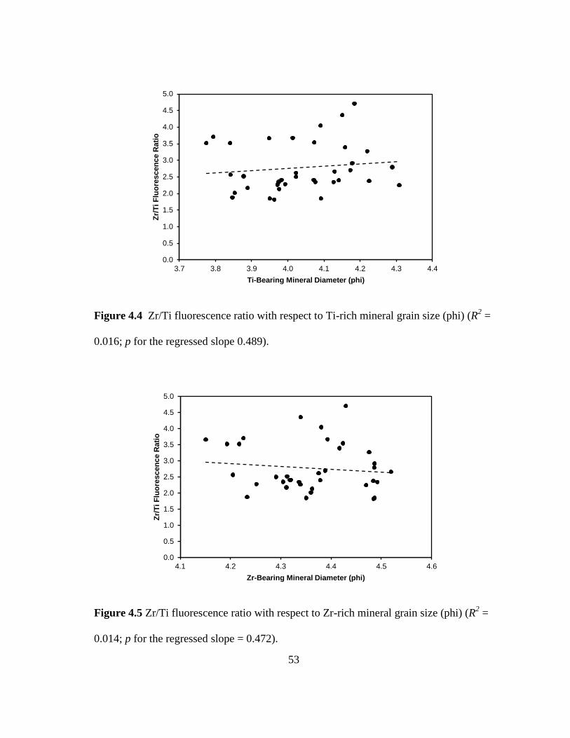
53

Figure 4.4 Zr/Ti fluorescence ratio with respect to Ti-rich mineral grain size (phi) (R2 =

0.016; p for the regressed slope 0.489).

Figure 4.5 Zr/Ti fluorescence ratio with respect to Zr-rich mineral grain size (phi) (R2 =

0.014; p for the regressed slope = 0.472).

0.0

0.5

1.0

1.5

2.0

2.5

3.0

3.5

4.0

4.5

5.0

3.7 3.8 3.9 4.0 4.1 4.2 4.3 4.4

Zr/

Ti F

luo

rescen

ce R

ati

o

Ti-Bearing Mineral Diameter (phi)

0.0

0.5

1.0

1.5

2.0

2.5

3.0

3.5

4.0

4.5

5.0

4.1 4.2 4.3 4.4 4.5 4.6

Zr/

Ti F

luo

rescen

ce R

ati

o

Zr-Bearing Mineral Diameter (phi)

54

4.3.2 Lamination Thickness

Alternating light gray laminae and darker gray/black laminae were horizontal and

parallel to each other. Black laminae were enriched in Fe (Fig. 4.6) allowing consistent

estimation of lamination thickness from 10 µm resolution XRF scans. All samples

showed positive correlations (positive -value; Table 4.1; Fig. 4.7), and nine of fifteen

samples had significant linear relationship between lamination thickness and Zr/Ti ratio

( < 0.05; Table 4.1). The remaining samples showed no significant relationship at the

95% confidence level; no negative correlations were observed.

Results from this research found that (1) both zircon and rutilated quartz grains

were well-sorted and normally distributed, (2) rutilated quartz grain sizes were

systematically correlated with zircon grain sizes, (3) neither zircon grain nor rutilated

quartz grain size correlated with Zr/Ti ratio, and (4) lamination thickness and Zr/Ti

fluorescence ratio had positive correlations.

55

Table 4.1 Linear regression and correlation analysis between lamination thickness and

Zr/Ti ratio. Lamination thickness and Zr/Ti ratio are positively correlated in every

sample.

Sample Slope -value of the Slope Correlation -value

1-3 0.152 0.007* 0.853

1-4 0.232 0.003* 0.863

1-5 0.087 0.273 0.402

1-6 0.223 0.018* 0.940

1-7 0.085 0.089 0.638

1-8 0.311 0.040* 0.831

1-9 0.081 0.310 0.338

2-1 0.095 0.012* 0.648

2-2 0.160 0.039* 0.626

2-3 0.107 0.320 0.443

3-1 0.065 0.185 0.485

3-2 0.119 0.050 0.754

3-3 0.126 0.017* 0.799

3-4 0.062 0.034* 0.670

3-5 0.214 0.002* 0.872

*Sample with linear regression between Zr/Ti fluorescence ratio and lamination

thickness at the 95% confidence interval or greater shown in bold.

56

Figure 4.6 Fe-rich bands occur along black laminae. A) MBC 1-5 rock sample. B) Fe-

fluorescence of MBC 1-5 rock sample.

1 cm

A B

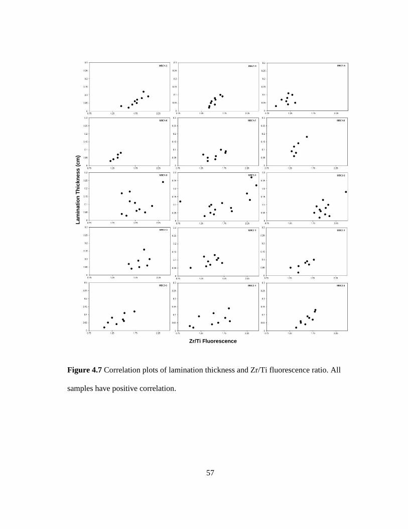
57

Figure 4.7 Correlation plots of lamination thickness and Zr/Ti fluorescence ratio. All

samples have positive correlation.

Zr/Ti Fluorescence

Ratio

La

min

ati

on

Th

ickn

ess (

cm

)

58


4.4.1 Sources of Zr/Ti Ratio Variation

Particles’ susceptibility to movement is highly influenced by grain size, shape,

packing, and sorting, and initial grain entrainment results from fluid drag and lift forces

on more exposed grains (Nickling, 1988). In a series of wind-tunnel experiments of dry

loose sand-sized sediments of a range of grain sizes, as wind velocity was slowly

increased, less exposed grains were moved by fluid drag force (Nickling, 1988). When

particle to fluid density ratio is low, the initial particle motion occurs at low fluid

velocity (Iversen et al., 1987). Thus, denser and smaller grains have lower susceptibility

to initial movement and require a relatively higher critical shear velocity to initiate

motion due to their lesser exposed surface area and higher particle to fluid density ratio.

Since zircon particles are smaller and denser than rutilated quartz particles (Fig.

4.3), zircon grains have lower susceptibility to particle movement. Variations in Zr/Ti

ratio are not correlated to grain size of either mineral (Fig. 4.4, 4.5). These observations

suggest that changes in Zr/Ti ratio did not result from varying in mineral grain sizes but

were likely from variations in mineral abundance. Consequently, high Zr/Ti ratios were

from increases in zircon abundance likely related to periods of enhanced erosion where

fluid speeds were high enough to move particles with lower susceptibility to movement.

Thicker lamination associated with high Zr/Ti ratio (Fig. 4.7); this is consistent to results

from Hu et al. (1999), Lückge et al. (2001), and Dean et al. (2002). Therefore, variations

in Zr/Ti ratio are, therefore, most likely derived from fluctuations in intensity of

erosional events.

59

4.5 CONCLUSIONS

Erosional event size during the deposition of thinly laminated siltstone in the

Brushy Canyon Formation was qualitatively analyzed from physical properties of zircon

and rutilated quartz. Zircon grains were systematically finer than rutilated quartz grains

but neither of these grain sizes was correlated with Zr/Ti fluorescence ratio. Also, Zr/Ti

fluorescence ratio and lamination thickness had positive correlations. Therefore,

fluctuations in Zr/Ti ratio were derived from changes in erosional intensity. The grain-

size distribution of these rock samples should be further analyzed in order to classify the

modes of transportation and deposition.

60

REFERENCES

Adams, J. E., 1936, Oil pool of open reservoir type: AAPG Bulletin, v. 20, no. 6, p. 780-

796.

Allen, J. R. L., 1991, The Bouma division A and the possible duration of turbidity

currents: Journal of Sedimentary Research, v. 61, no. 28, p. 291-295.

Amy, L. A., Talling, P. J., Edmonds, V. O., Sumner, E. J., and Lesueur, A., 2006, An

experimental investigation of sand-mud suspension settling behaviour:

implications for bimodal mud contents of submarine flow deposits:

Sedimentology, v. 53, no. 6, p. 1411-1434.

Bagnold, R. A., 1962, Auto-suspension of transported sediment: turbidity currents:

Proceedings of the Royal Society of London. Series A, Mathematical and

Physical Sciences, v. 265, no. 1322, p. 315-319.

Beaubouef, R. T., Rossen, C., Zelt, F. B., Sullivan, M. D., Mohrig, D. C., and Jennette,

D. C., 1999, Deep-water sandstones, Brushy Canyon Formation, west Texas,

AAPG Hedberg Field Research Conference.

Berthault, G., 1988, Experiments on lamination of sediments: EN Technology Journal, v.

3, p. 25-29.

Bouma, A. H., 1962, Sedimentology of some flysch deposits: a graphic approach to

facies interpretation, Amsterdam, Flsevier.

61

Bowen, A. J., Normark, W. R., and Piper, D. J. W., 1984, Modelling of turbidity currents

on Navy Submarine Fan, California Continental Borderland: Sedimentology, v.

31, no. 2, p. 169-185.

Brown, E. T., Johnson, T. C., Scholz, C. A., Cohen, A. S., and King, J. W., 2007, Abrupt

change in tropical African climate linked to the bipolar seesaw over the past

55,000 years: Geophysical Research Letters, v. 34, no. 20, p. L20702.

Chhabra, R. P., Agarwal, S., and Chaudhary, K., 2003, A note on wall effect on the

terminal falling velocity of a sphere in quiescent Newtonian media in cylindrical

tubes: Powder Technology, v. 129, no. 1, p. 53-58.

Davies, R., 1968, The experimental study of the differential settling of particles in

suspension at high concentrations: Powder Technology, v. 2, no. 1, p. 43-51.

Davis, H., R., Birdsell, and H., K., 1988, Hindered settling of semidilute monodisperse

and polydisperse suspensions, Hoboken, NJ, Wiley-Blackwell.

Dean, W. E., Forester, R. M., and Bradbury, J. P., 2002, Early Holocene change in

atmospheric circulation in the Northern Great Plains: an upstream view of the 8.2

ka cold event: Quaternary Science Reviews, v. 21, no. 16, p. 1763-1775.

Di Felice, R., 1996, A relationship for the wall effect on the settling velocity of a sphere

at any flow regime: International Journal of Multiphase Flow, v. 22, no. 3, p.

527-533.

Felix, M., 2002, Flow structure of turbidity currents: Sedimentology, v. 49, no. 3, p. 397-

419.

62

Fischer, A. G., and Sarnthein, M., 1988, Airborne silts and dune-derived sands in the

Permian of the Delaware Basin: Journal of Sedimentary Research, v. 58, no. 4, p.

637-643.

Glaccum, R. A., and Prospero, J. M., 1980, Saharan aerosols over the tropical North

Atlantic: mineralogy: Marine Geology, v. 37, no. 3, p. 295-321.

Gunderson, S., 2011, Early channel evolution in the Middle Permian Brushy Canyon

Formation, west Texas, USA. [Master] thesis, Texas A&M University, 35 p.

Harms, J. C., and Williamson, C. R., 1988, Deep-water density current deposits of

Delaware Mountain Group (Permian), Delaware Basin, Texas and New Mexico:

AAPG Bulletin, v. 72, no. 3, p. 299-317.

Haughton, P., Davis, C., McCaffrey, W., and Barker, S., 2009, Hybrid sediment gravity

flow deposits: classification, origin and significance: Marine and Petroleum

Geology, v. 26, no. 10, p. 1900-1918.

Hoyos, M., Bacri, J. C., Martin, J., and Salin, D., 1994, A study of the sedimentation of

noncolloidal bidisperse, concentrated suspensions by an acoustic technique:

Physics of Fluids, v. 6, no. 12, p. 3809-3817.

Hu, F., Slawinski, D., Wright, H., Ito, E., Johnson, R., Kelts, K., McEwan, R., and

Boedigheimer, A., 1999, Abrupt changes in North American climate during early

Holocene times: Nature, v. 400, no. 6743, p. 437-440.

Hull, J. P. D., 1957, Petrogenesis of Permian Delaware Mountain sandstone, Texas and

New Mexico: AAPG Bulletin, v. 41, no. 2, p. 278-307.

63

Iversen, J. D., Greeley, R., Marshall, J. R., and Pollack, J. B., 1987, Aeolian saltation

threshold: the effect of density ratio: Sedimentology, v. 34, no. 4, p. 699-706.

Jaenicke, R., and Schütz, L., 1978, Comprehensive study of physical and chemical

properties of the surface aerosols in the Cape Verde Islands region: Journal of

Geophysical Research: Oceans, v. 83, no. C7, p. 3585-3599.

Julien, P. Y., 1998, Erosion and Sedimentation, Cambridge, Cambridge University

Press.

Julien, P. Y., and Lan, Y., 1991, Rheology of hyperconcentrations: Journal of Hydraulic

Engineering, v. 117, no. 3, p. 346-353.

Kneller, B. C., and McCaffrey, W. D., 2003, The interpretation of vertical sequences in

turbidite beds: the influence of longitudinal flow structure: Journal of

Sedimentary Research, v. 73, no. 5, p. 706-713.

Komar, P. D., 1985, The hydraulic interpretation of turbidites from their grain sizes and

sedimentary structures: Sedimentology, v. 32, no. 3, p. 395-407.

Lowe, D. R., 1982, Sediment gravity flows II: depositional models with special

reference to the deposits of high-density turbidity currents: Journal of


Lückge, A., Doose-Rolinski, H., Khan, A. A., Schulz, H., and von Rad, U., 2001,

Monsoonal variability in the northeastern Arabian Sea during the past 5000

years: geochemical evidence from laminated sediments: Palaeogeography,

Palaeoclimatology, Palaeoecology, v. 167, no. 3, p. 273-286.

64

Machac , I., and ecjaks, Z., 1995, Wall effect for a sphere falling through a non-

Newtonian fluid in a rectangular duct: Chemical Engineering Science, v. 50, no.

1, p. 143-148.

Mackenzie, F. T., 2005, Sediments, diagenesis, and sedimentary rocks: treatise on

geochemistry, Elsevier Science.

Middleton, G. V., 1976, Hydraulic interpretation of sand size distributions: The Journal

of Geology, v. 84, no. 4, p. 405-426.

Middleton, G. V., and Southard, J. B., 1984, Mechanics of sediment movement.

Mulder, T., and Alexander, J., 2001, The physical character of subaqueous sedimentary

density flows and their deposits: Sedimentology, v. 48, no. 2, p. 269-299.

Nickling, W., 1988, The initiation of particle movement by wind: Sedimentology, v. 35,

no. 3, p. 499-511.

Nicolai, H., Herzhaft, B., Hinch, E. J., Oger, L., and Guazzelli, E., 1995, Particle

velocity fluctuations and hydrodynamic self‐diffusion of sedimenting non‐

Brownian spheres: Physics of Fluids, v. 7, no. 1, p. 12-23.

Oldfield, F., Wake, R., Boyle, J., Jones, R., Nolan, S., Gibbs, Z., Appleby, P., Fisher, E.,

and Wolff, G., 2003, The late-Holocene history of Gormire Lake (NE England)

and its catchment: a multiproxy reconstruction of past human impact: The

Holocene, v. 13, no. 5, p. 677-690.

Richardson, J. F., and Meikle, R. A., 1961, Sedimentation and fluidisation part III: the

sedimentation of uniform fine particles and of two-component mixtures of solids:

Transactions of the Institution of Chemical Engineers, v. 39, p. 348-356.

65

Richardson, J. F., and Zaki, W. N., 1954, Sedimentation and fluidisation: Part I:

Transactions of the Institution of Chemical Engineers, v. 32, p. S82-S100.

Riley, N. A., 1941, Projection sphericity: Journal of Sedimentary Research, v. 11, no. 28,

p. 94-95.

Roy, P. D., Rivero-Navarette, A., Lopez-Balbiaux, N., Pérez-Cruz, L. L., Metcalfe, S.

E., Sankar, G. M., and Sánchez-Zavala, J. L., 2013, A record of Holocene

summer-season palaeohydrological changes from the southern margin of

Chihuahua Desert (Mexico) and possible forcings: The Holocene, v. 23, no. 8, p.

1105-1114.

Rubey, W. W., 1933, The size distribution of heavy minerals within a water-laid

sandstone: Journal of Sedimentary Research, v. 3, no. 1, p. 3-29.

Schnetger, B., Brumsack, H. J., Schale, H., Hinrichs, J., and Dittert, L., 2000,

Geochemical characteristics of deep-sea sediments from the Arabian Sea: a high-

resolution study: Deep Sea Research Part II: Topical Studies in Oceanography, v.

47, no. 14, p. 2735-2768.

Segre, N., P., Liu, F., Umbanhowar, P., Weltz, and A., D., 2001, An effective

gravitational temperature for sedimentation: Nature, v. 409, no. 6820, p. 594-597.

Shaw, D. M., Watkins, N. D., and Huang, T. C., 1974, Atmospherically transported

volcanic glass in deep-sea sediments: theoretical considerations: Journal of

Geophysical Research, v. 79, no. 21, p. 3087-3094.

66

Silver, B. A., and Todd, R. G., 1969, Permian cyclic strata, northern Midland and

Delaware Basins, west Texas and southeastern New Mexico: AAPG Bulletin, v.

53, no. 11, p. 2223-2251.

Slingerland, R., and Smith, N. D., 1986, Occurrence and formation of water-laid placers:

Annual Review of Earth and Planetary Sciences, v. 14, no. 1, p. 113-147.

Slingerland, R. L., 1977, The effects of entrainment on the hydraulic equivalence

relationships of light and heavy minerals in sands: Journal of Sedimentary

Research, v. 47, no. 2, p. 753-770.

Steidtmann, J. R., 1982, Size-density sorting of sand-size spheres during deposition from

bedload transport and implications concerning hydraulic equivalence:

Sedimentology, v. 29, no. 6, p. 877-883.

Van Tassell, J., 1981, Silver abyssal plain carbonate turbidite: flow characteristics: The

Journal of Geology, v. 89, no. 3, p. 317-333.

Ver Straeten, C. A., Brett, C. E., and Sageman, B. B., 2011, Mudrock sequence

stratigraphy: a multi-proxy (sedimentological, paleobiological and geochemical)

approach, Devonian Appalachian Basin: Palaeogeography, Palaeoclimatology,

Palaeoecology, v. 304, no. 1, p. 54-73.

Visher, G. S., 1969, Grain size distributions and depositional processes: Journal of


Williamson, C. R., 1980, Sedimentology of Guadalupian deep-water clastic facies,

Delaware Basin, New Mexico and west Texas: New Mexico Geological Society

Guidebook, v. 31st Field Conference, p. 195-204.

mechanisms of sedimentation inferred from …

Documents