Mechanism and Machine Theory 118 (2017) 53–64

Contents lists available at ScienceDirect

Mechanism and Machine Theory

journal homepage: www.elsevier.com/locate/mechmachtheory

Research paper

Geometric analysis of coupler-link mobility and circuits for

planar four-bar linkages

Shaoping Bai

Department of Mechanical and Manufacturing Engineering, Aalborg University, Aalborg, Denmark

a r t i c l e i n f o

Article history:

Received 8 November 2016

Revised 25 May 2017

Accepted 29 July 2017

Keywords:

Four-bar linkage mobility analysis

Number of circuits

Range of rotation

Turning points

Constraint triangle

a b s t r a c t

The problem of mobility analysis of planar four-bar linkages is revisited. The mobility is

analyzed in terms of the range of coupler angle by a geometric approach, with a special

interest on its full rotatability when the linkage is driven by the coupler link. A constraint

triangle which characterizes the movement of the coupler link is constructed. By virtue of

the constraint triangle, a new formulation on the couple curve rotation is derived, upon

which the ranges of coupler angle are determined and the turning points are identified.

Moreover, with the range of coupler angle, the number of circuits is determined. Examples

are included to demonstrate the mobility analysis with the new approach.

© 2017 Elsevier Ltd. All rights reserved.

1. Introduction

The analysis and identification of the mobility, or more precisely, the intervals of rotation, of linkages is an important

aspect of the linkage design. As a classical problem in linkage design, mobility analysis was extensively addressed in lit-

eratures. In the reported works, the analyses were mostly conducted on the full mobility of a crank [1–3] . Basically, the

Grashof’s criterion can be used for the detection of a full rotatability. That means, for a planar four-bar linkage, the sum

of the shortest and longest link lengths cannot be greater than the sum of the remaining two link lengths if there is to be

continuous relative rotation between two members [4,5] . There are many other methods developed on the mobility analysis

to determine not only the full rotatability, but also the range of motion. Midha et al. [6] utilized the triangle inequality con-

cept to formulate the mobility conditions for planar four-bar linkages, and provided a graphical interpretation to mobility

determination. Angeles and Bernier proposed a unified method of mobility analysis based on the concept of linkage discrimi-

nant [7] . Most of these works addressed the mobility problem in terms of crank rotation, very few works are concerned with

the mobility of the coupler link.

The analysis of mobility of coupler link of planar linkages is important in both theory and applications. With the advances

of robotics, innovative designs of mechanisms are developed, where coupler-driven four-bar linkages are adopted [8–12] .

Coupler-driven linkages are also found their applications in novel transmission, energy converter etc [13,14] . An analysis

method focused on the mobility of the coupler link is needed for both design and analysis.

In this work, we address the mobility of the coupler-driven four-bar linkages. The constraint equations of four-bar link-

ages are reformulated and interpreted. A constraint triangle is constructed, which characterizes the movement of the coupler

link. By making use of the constraint triangle, a simple formulation is developed, with which the motion analysis is con-

ducted to determine the range of coupler rotation. Using the new formulation, the coupler’s full rotatability is re-evaluated.

E-mail addresses: shb@make.aau.dk , shb@m-tech.aau.dk

http://dx.doi.org/10.1016/j.mechmachtheory.2017.07.019

0094-114X/© 2017 Elsevier Ltd. All rights reserved.

54 S. Bai / Mechanism and Machine Theory 118 (2017) 53–64

Fig. 1. A coupler-driven four-bar linkage with revolute-revolute (RR) dyads, where φ is the coupler angle.

Fig. 2. Embodiments of coupler-driven four-bar linkages, (a) coupler-point driving with Revolute-Prismatic-Revolute (RPR) linkage, where the prismatic

joint is active, (b) coupler-angle driving with Prismatic-Prismatic-Revolute (PPR) linkage, where the revolute joint is active.

The problem of circuit number determination is studied. A method of tracing coupler curve with the coupler angle as pa-

rameter is also presented. The work in this paper extends the mobility analysis in [15] , with inclusion of circuit and branch

analysis, all being demonstrated with examples.

2. Coupler-driven four-bar linkage

A fully parametric four-bar linkage model is illustrated in Fig. 1 . Let the position vector of the coupler point P is r =[ x, y ] T , expressed in a frame F fixed to link BD . A local coordinate system X L –Y L , fixed to the coupler link with its origin at

point P , is also defined. The local coordinates of points A and C are given as a 0 = [ −m, −h ] T and c 0 = [ l 3 − m, −h ] T , where m

and h define the position of point P in the coupler link, and l 3 is the length of the coupler link. Two centers of the four-bar

linkage are B ( b 1 , b 2 ) and D ( d 1 , d 2 ), from which the length l 1 of the base link is calculated. The problem at hand is to find

the range of φ, the coupler angle in the literature [1] .

For the coupler-driven linkage, two driving methods are possible. One is that the coupler link is driven by an external

force, which pushes the coupler at a coupler point P and moves it following its coupler curve noted by �. An embodiment

of this type of actuation can be a RPR linkage, as shown in Fig. 2 a. The other one is that the coupler link is driven by an

external torque, which rotates the coupler following a prescribed function of coupler angle φ. An embodiment of this type

actuation can be a PPR linkage, as shown in Fig. 2 b. In this work, we consider the coupler angle as an input, which physically

S. Bai / Mechanism and Machine Theory 118 (2017) 53–64 55

corresponds to the PPR embodiment. In both embodiments, two links, AB and CD , each with one joint grounded, are driven

by the coupler link.

The mobility analysis of four-bar linkages is conventionally done with algebra approach, utilizing closure loop equations

of the linkage, as can be seen in the works on the crank rotatability [1] . When this approach is applied to the mobility

analysis of the coupler, however, the formulation is ended up with a very complicated function of the coupler rotation, as it

has to use an intermediate variable, normally the crank angle, which has to be eliminated finally. This makes it difficult to

find the range of rotation angle φ for a given set of linkage parameters. Alternatively, the four-bar linkage can be transformed

virtually into a new linkage in which the crank and the coupler swop, so the coupler mobility analysis problem is converted

into a problem of crank mobility analysis.

In this work, we attempt to analyze the coupler mobility directly with a new formulation, adopting a geometric approach

utilizing a constraint triangle, as described presently.

2.1. Constraint equations

We first formulate the constraint equations based on Burmester theory. Refer to Fig. 1 , the constraint equation for the

dyad BAP is

‖ (r + Qa 0 ) − b ‖

2 = l 2 2 (1)

where b is the position vector of point B in the fixed frame F . Moreover, Q denotes the rotation matrix carrying the coupler

link from its reference to its current orientation through an angle φ.

Eq. (1) implies that the trajectory of point A is a circle of radius l 2 , centered at point B . The equation can also be written

as

‖ r − (b − Qa 0 ) ‖

2 = l 2 2 (2)

which represents a circle centered at a point with position vector (b − Qa 0 ) , if Q is fixed. Similarly, the constraint equation

for the DCP dyad is

‖ r − (d − Qc 0 ) ‖

2 = l 2 4 (3)

where d is the position vector of point D in the fixed frame F . The equation represents a circle centered at a point with

position vector (d − Qc 0 ) , if Q is fixed.

Let

u = r − (b − Qa 0 ) , v = r − (d − Qc 0 ) (4)

which are two vectors parallel to AB and CD , with their lengths being equal to l 2 and l 4 , respectively. Subtracting Eq. (3) from

(2) yields

‖ u ‖

2 − ‖ v ‖

2 = l 2 2 − l 2 4 ; (5)

that is

(u + v ) · (u − v ) = l 2 2 − l 2 4 (6)

or

(2 r + Q (a 0 + c 0 ) − (b + d )) · (Q (a 0 − c 0 ) − (b − d )) = l 2 2 − l 2 4 (7)

which is a linear constraint of r . The geometric meanings are explained in next section.

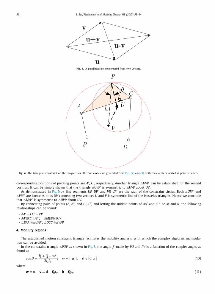
3. A triangle of motion constraint

Eq. (6) is a derived constraint from two basic link-length constraints (2) and (3) . The equation stands for a parallelogram

constructed with vectors u and v , for which u + v and u − v are exactly the diagonal vectors, as demonstrated in Fig. 3 .

The parallelogram leads to a vector triangle, constructed by u, v and u − v . An equivalent triangle is constructed with a

vertex at P , namely, � PUV , as shown in Fig. 4 .

It is clear that in the triangle the side lengths of PU and PV , which are the magnitudes of vectors u, v , are constant, equal

to l 2 and l 4 , respectively. We recall that the closure equation of the quadrilateral BACD can be expressed as

b + u + Q (c 0 − a 0 ) = d + v (8)

or

u − v = Q (a 0 − c 0 ) + d − b = (r + Qa 0 − b ) − (r + Qc 0 − d ) (9)

In other words, Eq. (4) defines the same geometric constraint as the closure loop equation. Thus the triangle � PUV charac-

terizes the movement of the coupler link.

For each given orientation of the coupler link, the coupler point of a four-bar linkage admits normally two solutions,

or two branches, which can be demonstrated in Fig. 5 (a). Let the other position of the coupler point P be noted by P ′ , the

56 S. Bai / Mechanism and Machine Theory 118 (2017) 53–64

Fig. 3. A parallelogram constructed from two vectors.

Fig. 4. The triangular constraint on the coupler link. The two circles are generated from Eqs. (2) and (3) , with their centers located at points U and V .

corresponding positions of pivoting points are A

′ , C ′ , respectively. Another triangle � UVP ′ can be established for the second

position. It can be simply shown that the triangle � UVP ′ is symmetric to � UVP about UV :

As demonstrated in Fig. 5 (b), line segments UP, UP ′ and VP, VP ′ are the radii of the constraint circles. Both � UPP ′ and

� VPP ′ are isosceles, thus UV connecting two vertices U and V is symmetric line of the isosceles triangles. Hence we conclude

that � UVP ′ is symmetric to � UVP about UV .

By connecting pairs of points ( A, A

′ ) and ( C, C ′ ) and letting the middle points of AA

′ and CC ′ be M and N , the following

relationships can be found:

• AA

′ = C C ′ = P P ′ • AA

′ ‖ CC ′ ‖ PP ′ ; BM ‖ DN ‖ UV

• � BAA

′ ∼=

� UPP ′ ; � DCC ′ ∼=

� VPP ′

4. Mobility regions

The established motion constraint triangle facilitates the mobility analysis, with which the complex algebraic manipula-

tion can be avoided.

In the constraint triangle � PUV as shown in Fig. 5 , the angle β made by PU and PV is a function of the coupler angle, as

found as

cos β =

l 2 2 + l 2 4 − w

2

2 l 2 l 4 ; w = || w || , β ∈ [0 , π ] (10)

where

w ≡ u − v = d + Qa 0 − b − Qc 0 (11)

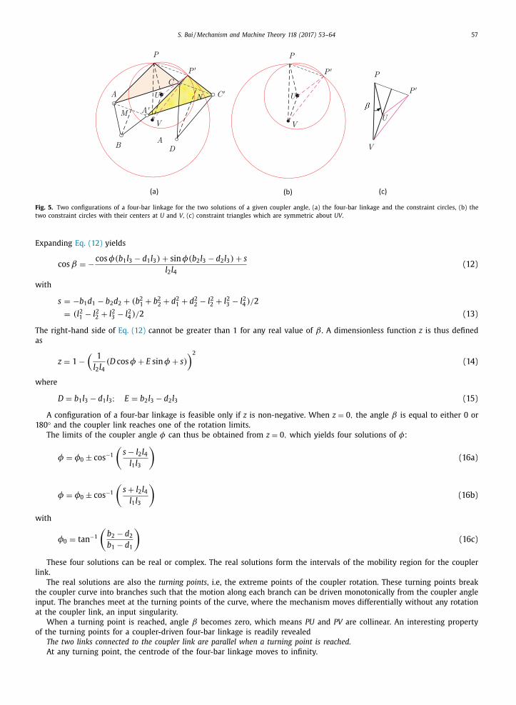
S. Bai / Mechanism and Machine Theory 118 (2017) 53–64 57

Fig. 5. Two configurations of a four-bar linkage for the two solutions of a given coupler angle, (a) the four-bar linkage and the constraint circles, (b) the

two constraint circles with their centers at U and V , (c) constraint triangles which are symmetric about UV .

Expanding Eq. (12) yields

cos β = −cos φ(b 1 l 3 − d 1 l 3 ) + sin φ(b 2 l 3 − d 2 l 3 ) + s

l 2 l 4 (12)

with

s = −b 1 d 1 − b 2 d 2 + (b 2 1 + b 2 2 + d 2 1 + d 2 2 − l 2 2 + l 2 3 − l 2 4 ) / 2

= (l 2 1 − l 2 2 + l 2 3 − l 2 4 ) / 2 (13)

The right-hand side of Eq. (12) cannot be greater than 1 for any real value of β . A dimensionless function z is thus defined

as

z = 1 −(

1

l 2 l 4 (D cos φ + E sin φ + s )

)2

(14)

where

D = b 1 l 3 − d 1 l 3 ; E = b 2 l 3 − d 2 l 3 (15)

A configuration of a four-bar linkage is feasible only if z is non-negative. When z = 0 , the angle β is equal to either 0 or

180 ° and the coupler link reaches one of the rotation limits.

The limits of the coupler angle φ can thus be obtained from z = 0 , which yields four solutions of φ:

φ = φ0 ± cos −1

(s − l 2 l 4

l 1 l 3

)(16a)

φ = φ0 ± cos −1

(s + l 2 l 4

l 1 l 3

)(16b)

with

φ0 = tan

−1

(b 2 − d 2 b 1 − d 1

)(16c)

These four solutions can be real or complex. The real solutions form the intervals of the mobility region for the coupler

link.

The real solutions are also the turning points , i.e, the extreme points of the coupler rotation. These turning points break

the coupler curve into branches such that the motion along each branch can be driven monotonically from the coupler angle

input. The branches meet at the turning points of the curve, where the mechanism moves differentially without any rotation

at the coupler link, an input singularity.

When a turning point is reached, angle β becomes zero, which means PU and PV are collinear. An interesting property

of the turning points for a coupler-driven four-bar linkage is readily revealed

The two links connected to the coupler link are parallel when a turning point is reached.

At any turning point, the centrode of the four-bar linkage moves to infinity.

58 S. Bai / Mechanism and Machine Theory 118 (2017) 53–64

5. Analysis of the mobility region

We will look into Eqs. (16a) and (16b) on different cases of solutions and to analyze further the mobility of a coupler

link. Depending on the linkage parameters, the equation can admit four, two or zero real solutions.

We first find conditions leading to real solutions. For inverse cosine functions, the argument has to be not great than 1,

which means

(s − l 2 l 4 ) 2 ≤ (l 1 l 3 )

2 or (s + l 2 l 4 ) 2 ≤ (l 1 l 3 )

2 (17)

The first inequality, upon considering the inequality of lengths of quadrilaterals, finally yields

l 1 + l 3 ≥ l 2 + l 4 (18)

The second inequality leads to

(l 1 − l 3 ) 2 ≤ (l 2 − l 4 )

2 (19)

Three cases are thus identified with respect to inequalities (18) and (19)

1. Case 1: both inequalities are satisfied. There are four real solutions, or four turning points. On the plot of z vs φ, there

are two intervals of feasible coupler angle.

2. Case 2: only one of the two inequalities is satisfied. There are two real solutions, or two turning points. On the plot of z

vs φ, there is only one interval of feasible coupler angle.

3. Case 3: none of the two inequalities are satisfied. There is no real solutions, or no turning points can be identified. On

the plot of z vs φ, the interval of feasible coupler angle is unbounded.

5.1. Condition for a full rotation of the coupler link

The condition for a linkage with a full rotation of the coupler link can be derived from Case 3. In Case 3, the limit

equation of coupler equation admits no real solutions, which means no limits exist for the coupler link rotation, and thus

the linkage can make a full, or unbounded rotation of the coupler link. Moreover, in a special condition of Case 2, when the

mobility range is found exactly as 2 π , the mechanism admits also a full coupler rotation.

5.1.1. Case 3

In this case, the conditions admitting no real solutions are

(l 1 − l 3 ) 2 > (l 2 − l 4 )

2 (20)

and

l 1 + l 3 < l 2 + l 4 (21)

A careful analysis of both inequalities for different combinations of the shortest and longest links has been done. The analysis

result, as listed in Appendix for all 12 combinations, reveals that, if we assign the shortest link to either the coupler or the

grounded link, a full coupler rotatability is obtained. There are totally six combinations of which the coupler link can make

a full rotation.

5.1.2. A special condition of Case 2

When Eq. (18) takes the equal sign, the inverse cosine function has solutions of ±π . The range of rotation is exactly

equal to 360 °. This means a Grashof linkage with fully rotatable coupler link is still possible.

The above two cases are the Grashof conditions applicable for the coupler link. It is noted that in literature there are four

types of Grashof linkages, namely, double-crank, crank-rocker, rocker-crank and Grashof double-crank types, depending on

the relative rotations of two neighboring links. Of them, we can find from our results that double-rocker and double-crank

types of Grashof linkages allow a full rotation of the coupler, as shown in the Appendix .

With the results above, it is thus clear for the condition of full coupler rotatability:

The coupler link is fully rotatable if and only if either the coupler or the grounded link is the shortest one of a Grashof linkage.

A mathematical proof of the Grashof’s criterion by means of polynomial discriminant was presented in [16] , taking the

crank angle as the rotation variable. In this work, we use the coupler angle as variable for the proof of coupler’s full rotation.

In this regard, the current work can be considered as complementary to the proof in [16] .

5.2. The number of circuits

Another part of the mobility analysis deals with circuits, branches and turning points, as they provide movement state

changes of linkages.

A circuit, also known as assembly mode, of a linkage is defined as all possible orientations of the output link of the

linkage, or all possible positions of a coupler point, which can be realized without disconnecting any joints [17] . The turning

points are also referred as input singularities. In this work, the coupler angle is used as input variable. At the turning points,

S. Bai / Mechanism and Machine Theory 118 (2017) 53–64 59

Table 1

Number of circuits in four-bar linkages.

No. solutions intervals circuits linkage conditions

1 4 2 2 non-Grashof (l 1 − l 3 ) 2 ≤ (l 2 − l 4 )

2 and l 1 + l 3 ≥ l 2 + l 4 2 2 1 1 Grashof (l 1 − l 3 )

2 > (l 2 − l 4 ) 2 and l 1 + l 3 = l 2 + l 4

1 1 non-Grashof (l 1 − l 3 ) 2 ≤ (l 2 − l 4 )

2 or l 1 + l 3 ≥ l 2 + l 4 3 0 0 2 Grashof (l 1 − l 3 )

2 > (l 2 − l 4 ) 2 and l 1 + l 3 < l 2 + l 4

the two branches meet and the angular velocity of the coupler link vanishes. Moreover, the crank and the follower are

parallel, a configuration allowing instantaneous translation. It is noted that the turning points in the coupler driven linkage

are different from the crank-driven linkages. In the latter case, the coupler becomes collinear with either the crank or the

follower when a turning point is reached [17,18] .

A method to determine the number of circuits was developed in [19] , in which the image curve of the coupler movement

in a kinematic image space was checked. The method reached the same conclusion as that in the book of Erdman, Sandor

and Kota [20] . However, the conclusion is not accurate, as we find later. In this work, we try to determine directly the

number of circuits by checking the number of intervals of coupler rotation, taking into consideration of branches.

It is a known fact that there are two solutions of coupler point location for a given coupler angle. The two solutions cor-

respond to two branches. This fact, combining with different number of intervals of the coupler angle, yields the following

results on the number of circuits:

• Two intervals . They are formed by four turning points. In each interval, there exist two pieces of coupler curves, corre-

sponding to the two branches. The two pieces of curves meet at two turning points, where the coupler point changes

branches. The connected curves form as one curve, or one circuit. So two intervals end up with two circuits.

• One interval , or two turning points. With the same token, one interval ends up with one circuit only.

• Zero interval , or no turning points. There exist two curves for the two branches. As there are no turning points on the

curve, the two curves has no turning points in common to meet each other. Each curve forms separately a circuit for

one branch. The coupler curve thus has two circuits.

From the above analysis, it is clear that a coupler curve has one circuit if and only if there is only one feasible range of

angle rotation, which corresponds to Case 2.

A special case of Case 2 is noted. In Case 2, when Eq. (18) takes the equal sign, the inverse cosine function has two

solutions of −π and π . There is still one interval of feasible coupler angle, which is exactly equal to 360 °. In other words,

the coupler link rotates for 360 ° in one branch, and 720 ° in its two branches of a circuit.

The above results are summarized in Table 1 .

In the literatures [19,20] , it was stated that non-Grashof linkages have one circuit (assembly mode), while all Grashof

linkages have two circuits. This statement, however, is inaccurate. From Table 1 , we can see that a Grashof linkage can have

one circuit, if the sum of two pairs of opposite links are identical. This will be further demonstrated in Section 7 .

6. Coupler curve tracing

The identified turning points are useful for coupler curve tracing. A parametric coupler curve equation can be established

in terms of coupler angle φ, paying attention to the turning points where branch changes. Referring to Fig. 4 , the coordinate

of a coupler point P can be obtained as

r P = d − Q (φ) c 0 − l 4 R (±α) ̂ w , α = cos −1 l 2 4 + w

2 − l 2 2

2 wl 4 (22)

where ˆ w is the unit vector parallel to w , and R ( ±α) is a rotation matrix of angle ±α, the angle made by VU and VP . Eq.

(22) expresses the two branches of the coupler point, where the branch, indicated by the sign of α, changes only a turning

point is reached.

Note Eq. (22) takes use of the dyad DCP . Alternatively, it can also take use of the dyad BAP and yield the same result.

Eq. (22) stands also for a parametric coupler-curve equation. A coupler curve can thus be traced using this equation.

The coupler curve tracing is not a simple problem due to the high-order polynomial and singularities [18] . A method by

distance geometry was proposed in [21] . Comparing to that one, the method proposed above is simpler and straight forward.

7. Examples

We first include three examples to demonstrate the mobility analysis with the new formulation. The linkage parameters

are given in Table 2 . The two sets of parameters are taken from [22] .

60 S. Bai / Mechanism and Machine Theory 118 (2017) 53–64

Table 2

Linkage parameters for Examples 1, 2 and 3 (units: m).

Ex. m h [ b 1 , b 2 ] [ d 1 , d 2 ] l 2 l 3 l 4

1 0.1 0.15 [ −0 . 2 , 0] [0 . 2 , −0 . 2] 0.15 0.4 0.35

2 0.083 −0 . 125 [ −0 . 2 , 0] [ −0 . 025 , 0 . 1] 0.180 0.068 0.157

3 0.1 0.0 [0, 0] [0.25, 0] 0.2 0.3 0.2

Fig. 6. Mobility analysis of Example 1, (a) plot of z vs φ, where the shadow areas show the ranges of rotation, (b) turning points on the coupler curve.

7.1. Example 1

In the first example, the linkage parameters take values from the first data set in Table 2 . The ranges of coupler rotation

are found as φ ∈ [ −2 . 432 , −1 . 520] rad and φ ∈ [ −0 . 334 , 0 . 577] rad from Eqs. (16a) –(16b) . The plot of z function is shown in

Fig. 6 (a), in which two distinct intervals of coupler angle are clearly displayed.

The above boundaries of the motion range are the turning points of the coupler link. Fig. 6 (b) displays the turning points

on the coupler curve, along with the four-bar linkage. It is seen that the four turning points are on two circuits of the

coupler curve, each circuit corresponding to one range of rotation. For this linkage, while the Grashof’s criterion is satisfied,

it allows a full rotation of the crank, but not the coupler link.

7.2. Example 2

The second example takes the second set of linkage parameters in Table 2 , which is actually a cognate linkage of the

four-bar linkage in the first example. The limit equations (16a) –(16b) have no real solutions, which means that function

z has not intersection with φ-axis, as shown in Fig. 7 (a). In other words, the coupler link can generate a full rotation. No

turning points exist for this linkage, as seen in Fig. 7 (b). For this linkage, inequality (21) becomes the Grashof criterion, while

inequality (20) is satisfied too.

7.3. Example 3

One more example is given for a four-bar Watt linkage [23] . Only two turning points exist, which are φ =[ −1 . 6208 , 1 . 6208] rad , corresponding to one interval. So the linkage has only one circuit, as shown in Fig. 8 .

The above three examples show different coupler curves, which lead to rotatability in different ranges. By virtue of plot of

constraint manifolds, the rotatability can be explained readily. Fig. 9 displays three manifolds of the examples. The manifold

is constructed with the constraint Eqs. (2) and (3) . Maple’s 3-D surface plot function implicitplot3d was utilized to

generate the surfaces. Another command intersectplot was used to obtain the intersections. In the manifolds, each

cross-section in the x –y plane contains two constraint circles for a fixed coupler angle. The entire manifold plots allow us to

observe directly the coupler rotatability either in a full rotation and a limited range of rotation, and the number of circuits.

The turning points on the intersections of the manifolds are the extremes of φ, which can be easily identified.

As can be seen from the first example, the constraint manifolds have two intersections, which are two closed-curve in

3-D space. The turning points of the linkage are the extreme points of the two curves, where the coupler angle reaches

either their maximum and minimum. In the second example, the two manifolds intersection yields to two open curves, no

S. Bai / Mechanism and Machine Theory 118 (2017) 53–64 61

Fig. 7. Mobility analysis of Example 2, (a) plot of z vs φ, (b) the linkage and the coupler curve, where no turning points can be identified.

Fig. 8. Example 3 of one-circuit linkage, (a) two turning points and the linkage, (b) plot of z vs φ, showing the range of motion.

extreme points, or turning points, can be identified. The linkage thus can rotate fully. In the example of the four-bar Watt

linkage, the intersection yields only one closed curve. The linkage has thus one circuit accordingly.

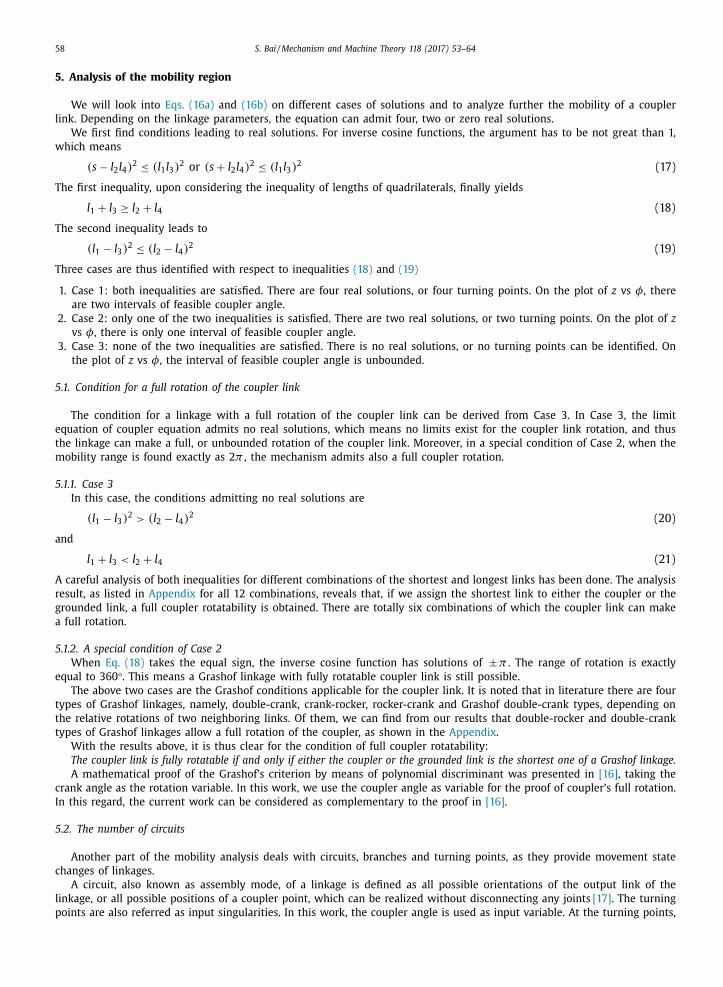
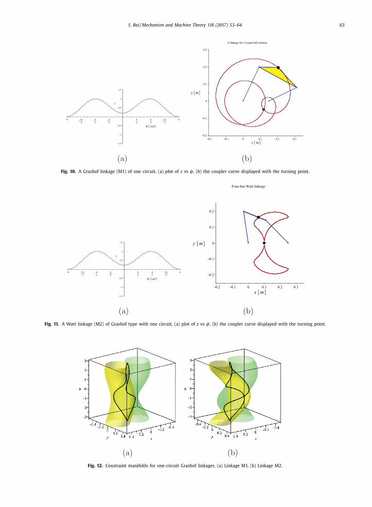
7.4. Grashof linkages of one circuit

We include two more examples to demonstrate the determination of number of circuits and to support our conclusion

that one circuit exists for Grashof linkages too. For two linkages with link parameters given in Table 3 , we can easily deter-

mine that they have only one circuit (assembly mode), using inequalities in Table 1 . Both linkages, as shown in Figs. 10 and

11 , are Grashof linkages and their range of coupler angle rotation is exactly equal to 360 °. On each coupler curve, there is

only one turning point. A tracing on the whole coupler curve generates 720 ° of rotation of the coupler. Both the only circuit

and the 720 ° rotation can be observed from the manifold plots in Fig. 12 . The turning points shown on the manifold plots

are located at φ = ±πrad, thus yield only one overlapped turning point in the coupler curves.

8. Conclusions

In this paper, the motion analysis is studied for the coupler link of planar four-bar linkages, addressing the need of

designing coupler-driven linkages. By means of a motion constraint triangle, the coupler motion is analyzed to yield the

62 S. Bai / Mechanism and Machine Theory 118 (2017) 53–64

Fig. 9. Constraint manifolds and their intersections, (a) Example 1 with two ranges of rotations, (b) Example 2 having a full rotation, (c) Example 3 of a

four-bar Watt linkage. In all examples, the number of circuits and turning points can be intuitively identified.

Table 3

Linkages of one circuit (units: m).

No. m h [ b 1 , b 2 ] [ d 1 , d 2 ] l 2 l 3 l 4

M1 0.1 0.05 [0.0, 0.0] [0.15, 0.0] 0.22 0.25 0.18

M2 0.1 0.0 [0.0, 0.0] [ −0 . 25 , 0 . 0] 0.2 0.15 0.2

range of coupler angle. With the new formulation the conditions for the full coupler rotatability are re-evaluated. Moreover,

the linkage circuits and coupler curve tracing are studied.

A contribution of this work is the construction of the motion constraint triangle, which facilitates the four-bar link-

age motion analysis. Comparing with the conventional constraint triangle constructed by connecting two diagonal vertices,

the constraint triangle is more comprehensive and able to capture to motion features of four-bar linkages. With the con-

straint triangle, the mobility of the coupler like is analyzed. Moreover, the conditions for a full rotation of a coupler link are

checked. It is shown clearly that either the coupler or the ground link has to be the shortest one in a Grashof linkage to

enable a full coupler rotation.

S. Bai / Mechanism and Machine Theory 118 (2017) 53–64 63

Fig. 10. A Grashof linkage (M1) of one circuit, (a) plot of z vs φ, (b) the coupler curve displayed with the turning point.

Fig. 11. A Watt linkage (M2) of Grashof type with one circuit, (a) plot of z vs φ, (b) the coupler curve displayed with the turning point.

Fig. 12. Constraint manifolds for one-circuit Grashof linkages, (a) Linkage M1, (b) Linkage M2.

64 S. Bai / Mechanism and Machine Theory 118 (2017) 53–64

Another contribution of the work includes the determination of the number of circuits. A four-bar linkage’s coupler curve

has only one circuit if the linkage has only one range of limited rotation or exactly 360 °. The corresponding conditions with

link lengths are expressed explicitly. Both Grashof and non-Grashof linkages can have one circuit. The result in this work

corrects the inaccurate statement in the literatures on the number of circuits of linkages.

The results of this work can be applied to design synthesis, for example, the conditions of full rotation or reaching to a

certain range. The results can also be useful for circuit defect detection and avoidance. For example, in the linkage design,

additional constraints can be included in synthesis to generate a linkage of one circuit, for which possible circuit defect can

be avoided.

Appendix. Rotatability of the coupler link in four-bar linkages

Table 4

Condition checking for full coupler rotation (FCR).

l min l max FCR? simplified Eq. (21) remarks

l 1 l 2 Y l 1 + l 2 < l 3 + l 4 both equations are satisfied; Eq. (21) is the Grashof Criterion

l 3 Y l 3 − l 1 > | l 2 − l 4 | both equations are satisfied; Eq. (22) is the Grashof Criterion

l 4 Y l 3 − l 1 > l 4 − l 2 both equations are satisfied; Eq. (21) is the Grashof Criterion

l 2 l 1 N l 1 − l 3 < l 4 − l 2 Eq. (22) cannot be satisfied

l 3 N l 3 − l 1 > l 4 − l 2 Eq. (22) cannot be satisfied

l 4 N l 4 − l 2 < | l 1 − l 3 | Eq. (21) cannot be satisfied

l 3 l 1 Y l 1 − l 3 > | l 4 − l 2 | both equations are satisfied; Eq. (22) is the Grashof Criterion

l 2 Y l 1 − l 3 > l 2 − l 4 both equations are satisfied; Eq. (21) is the Grashof Criterion

l 4 Y l 1 − l 3 > l 4 − l 2 both equations are satisfied; Eq. (21) is the Grashof Criterion

l 4 l 1 N l 2 + l 3 < l 1 − l 4 Eq. (21) is the Grashof criterion, Eq. (22) cannot be satisfied

l 2 N l 2 − l 4 < | l 1 − l 3 | Eq. (21) cannot be satisfied

l 3 N l 1 + l 2 < l 3 + l 4 Eq. (22) cannot be satisfied

References

[1] J.M. McCarthy , G.S. Soh , Geometric Design of Linkages, Springer, New York, 2011 .

[2] C. Innocenti , et al. , Analytical determination of the intersections of two coupler-point curves generated by two four-bar linkages, in: J. Angeles (Ed.),

Computational Kinematics, volume 28, 1993, pp. 251–262 . [3] S. Bai , J. Angeles , Coupler-curve synthesis of four-bar linkages via a novel formulation, Mech. Mach. Theory 94 (2015) 177–187 .

[4] F. Grashof , Theoretische maschinenlehre: Bd. theorie der getriebe und der mechanischen messinstrumente, Theoretische Maschinenlehre, L. Voss, 1883 .[5] W. Steinhilper , H. Hennerici , S. Britz , Kinematische Grundlagen Ebener Mechanismen Und Getriebe, Vogel, Würzburg, 1993 .

[6] A. Midha , Z.-L. Zhao , I. Her , Mobility conditions for planar linkages using triangle inequality and graphical interpretation, ASME J. Mech. Des. 107 (3)(1985) 394–399 .

[7] J. Angeles , A. Bernier , A general method of four-bar linkage mobility analysis, ASME J. Mech. Des. 109 (2) (1987) 197–203 .

[8] C.W. Radcliffe , Four-bar linkage prosthetic knee mechanisms: kinematics, alignment and prescription criteria, Prosthet. Orthot. Int. 18 (3) (1994)159–173 .

[9] A. Hamon , Y. Aoustin , Cross four-bar linkage for the knees of a planar bipedal robot, in: 2010 10th IEEE-RAS Inter. Conf. on Humanoid Robots (Hu-manoids), 2010, pp. 379–384 .

[10] R. Zbikowski , C. Galinski , C.B. Pedersen , Four-bar linkage mechanism for insectlike flapping wings in hover: concept and an outline of its realization,ASME J. Mech. Des. 127 (4) (2005) 817–824 .

[11] J. Chu , W. Cao , Synthesis of coupler curves of planar four-bar linkages through fast fourier transform, Chin. J. Mech. Eng. 29 (5) (1993) 117–122 .

[12] M. Lyu , W. Chen , X. Ding , J. Wang , S. Bai , H. Ren , Design of a biologically inspired lower limb exoskeleton for human gait rehabilitation, Rev. Sci.Instrum. 87 (10) (2016) .

[13] J.-W. Kim , J. Bak , T. Seo , J. Kim , New angular transmission design based on a four-bar linkage mechanism, in: Proc. ASME DETC2015, 2015 . Boston,USA, #DETC2015-46146.

[14] M. Dosaev , L. Klimina , Y. Selyutskiy , in: Wind Turbine Based on Antiparallel Link Mechanism, Springer International Publishing, Cham, 2017,pp. 543–550 .

[15] S. Bai , in: Coupler-Link Mobility Analysis of Planar Four-Bar Linkages, Springer International Publishing, Cham, 2017, pp. 41–49 . [16] R.L. Williams , C.F. Reinholtz , Proof of Grashof’s law using polynomial discriminants, ASME. J. Mech. Trans. Autom. 108 (4) (1986) 562–564 .

[17] T.R. Chase , J.A. Mirth , Circuits and branches of single-degree-of-freedom planar linkages, AMSE J. Mech. Des. 115 (2) (1993) 223–230 .

[18] D.H. Myszka , A.P. Murray , C.W. Wampler , Mechanism branches, turning curves, and critical points, in: ASME IDETC2012, 2012, pp. 1513–1525 . [19] H.P. Schröcker , M. Husty , J.M. McCarthy , Kinematic mapping based assembly mode evaluation of planar four-bar mechanisms, ASME. J. Mech. Des. 129

(9) (2006) 924–929 . [20] A.G. Erdman , G.N. Sandor , S. Kota , Mechanism Design: Analysis and Synthesis, 1, fourth ed., Prentice Hall, Upper Saddle River, New Jersey, 2001 .

[21] N. Rojas , F. Thomas , Application of distance geometry to tracing coupler curves of pin-jointed linkages, ASME J. Mech. Rob. 5 (2) (2013) .021001.1–021001.9.

[22] S. Bai , in: Determination of Linkage Parameters from Coupler Curve Equations, Springer International Publishing, Cham, 2015, pp. 49–57 .

[23] J.W. Rutter , Geometry of Curves, Chapman and Hall/CRC, 20 0 0 .