mechanical systems and signal processing - gipsa-lab.frpierre.granjon/doc/publi/artmssp17b.pdf ·...

Estimation of geometric properties of three-component signalsfor system monitoring

Pierre Granjon ⇑, Gailene Shih Lyn PhuaUniv. Grenoble Alpes, GIPSA-Lab, F-38000 Grenoble, FranceCNRS, GIPSA-Lab, F-38000 Grenoble, France

a r t i c l e i n f o

Article history:Received 1 September 2016Received in revised form 29 March 2017Accepted 2 April 2017Available online 12 April 2017

Keywords:Three-component signalsGeometric propertiesFrenet-Serret frameBearing faultsVoltage dipsCondition monitoring

a b s t r a c t

Most methods for condition monitoring are based on the analysis and characterization ofphysical quantities that are three-dimensional in nature. Plotted in a three-dimensionalEuclidian space as a function of time, such quantities follow a trajectory whose geometriccharacteristics are representative of the state of the monitored system. Usual conditionmonitoring techniques often study the measured quantities component by component,without taking into account their three-dimensional nature and the geometric propertiesof their trajectory. A significant part of the information is thus ignored. This article detailsa method dedicated to the analysis and processing of three-component quantities, capableof highlighting the special geometric features of such data and providing complementaryinformation for condition monitoring. The proposed method is applied to two experimen-tal cases: bearing fault monitoring in rotating machines, and voltage dips monitoring inthree-phase power networks. In this two cases, the obtained results are promising andshow that the estimated geometric indicators lead to complementary information thatcan be useful for condition monitoring.

! 2017 Elsevier Ltd. All rights reserved.

1. Introduction

Safety and economical constraints force industries to continuously improve their maintenance strategies. When possible,predictive or condition-based maintenance is used as it helps reducing repair time and cost, improve safety, and avoid eco-nomic losses. Very often, condition monitoring techniques rely on the characterization of inherently three-component phys-ical quantities, which are frequently encountered in technological processes. A first example is the monitoring of three-phaseelectrical systems, based on three-phase electrical measurements like voltages and currents. Another common example isthe monitoring of mechanical systems, based on three-axis vibration or three-dimensional displacement measurements.In order to obtain efficient fault indicators, such three-component signals are usually analyzed with the usual marginaland/or joint analysis tools in the time domain (correlation functions and/or correlation matrices) as well as in the frequencydomain (spectra and/or spectral matrices) [1]. However, three-component signals also contain another type of informationwhich is completely different in nature: their geometric properties. When a three-component signal is represented inthree-dimensional Euclidean space, it follows a particular trajectory. The geometric properties of this trajectory may containinformation concerning the state of the monitored system from which the signal was acquired. This approach has alreadybeen successfully proposed in the field of system monitoring with two-component signals [2] by using complex-valued

http://dx.doi.org/10.1016/j.ymssp.2017.04.0020888-3270/! 2017 Elsevier Ltd. All rights reserved.

⇑ Corresponding author at: Univ. Grenoble Alpes, GIPSA-Lab, F-38000 Grenoble, France.E-mail addresses: [email protected] (P. Granjon), [email protected] (G.S.L. Phua).

Mechanical Systems and Signal Processing 97 (2017) 95–111

Contents lists available at ScienceDirect

Mechanical Systems and Signal Processing

journal homepage: www.elsevier .com/locate /ymssp

http://crossmark.crossref.org/dialog/?doi=10.1016/j.ymssp.2017.04.002&domain=pdf

http://dx.doi.org/10.1016/j.ymssp.2017.04.002

mailto:[email protected]

mailto:[email protected]

http://dx.doi.org/10.1016/j.ymssp.2017.04.002

http://www.sciencedirect.com/science/journal/08883270

http://www.elsevier.com/locate/ymssp

signal processing tools [3]. It is for example the case for orbit shape analysis used to detect faults in rotating machines [4–6],and for voltage dips detection and classification in power networks [7]. However, and as previously mentioned, usual con-dition monitoring methods do not take into account the three-dimensional geometric characteristics of the trajectory of themeasured three-component quantities. As a consequence, a significant part of the diagnostic information is ignored.

This research work aims to fill this gap by developing a method to estimate the geometric properties of three-componentsignals which takes into account all three components at the same time. The proposed method relies on basic concepts ofdifferential geometry of space curves such as the Frenet-Serret frame and formulas, curvature and torsion, and leads to localgeometric descriptors of the three-dimensional curves followed by three-component signals. The method takes as its input athree-component signal, i.e. a time series where three data points are available at each time t. These data are then consideredas Cartesian coordinates defining the position of the measured signal at time t in a three-dimensional Euclidean space. How-ever, raw signals measured in real-life systems tend to be complicated and thus lead to trajectories with complicated geo-metric properties. To simplify matters, as in spectral analysis, the signal is simplified by analyzing only one frequencycomponent. This sinusoidal signal, composed of three sinusoids of the same frequency, follows a trajectory in three-dimensional space which is elliptical in shape, and the geometric properties of the corresponding trajectory can be analyzedmore easily. This is what the proposed method is for: to estimate the geometric properties of the trajectory of a three-component sinusoidal signal in three-dimensional space. The estimated geometric properties can then be used to elaboratestand-alone or complementary fault indicators for condition monitoring purposes.

In order to validate this approach, the proposed method is applied to two different experimental cases: voltage dips mon-itoring in three-phase power networks, and bearing faults monitoring in rotating machines. In this two cases, the resultsobtained are promising and show that the estimated geometric indicators lead to complementary information that can beuseful for condition monitoring purpose.

The previous ideas are detailed in this article, which is organized as follows. The theoretical foundations of the proposedmethod are presented in Section 2, which includes the basic differential geometry tools used, the definition of the three-component signal of interest, as well as the geometric properties to be estimated. The structure of the algorithm developedto estimate these geometric properties is then described in Section 3, along with the details of its estimation performancewith respect to various parameters. The experimental results obtained by this algorithm in the context of the two applicationexamples of voltage dips monitoring in three-phase power networks and bearing faults monitoring in rotating machines aregiven in Sections 4 and 5 respectively. Finally, the article ends with concluding remarks including a summary and sugges-tions of possible future work.

2. Geometric properties of three-component sinusoidal signals

2.1. Differential geometry of space curves

A natural way of defining a curve is through differentiable functions. Let I be an open interval in the real line R and r be afunction from I to R3 as defined in Eq. (1) where R3 denotes the set of triples of real numbers and r1; r2 and r3 are differen-tiable functions of t.

r : I ! R3

t # r1 tð Þ; r2 tð Þ; r3 tð Þð Þ ð1Þ

r is called a parametrized differentiable curve and the variable t is the parameter of the curve [8,9]. A curve r maps each t in Iinto a point r tð Þ ¼ r1 tð Þ; r2 tð Þ; r3 tð Þð Þ in R3 in such a way that the functions r1; r2 and r3 are differentiable. In other words, ateach t in some open interval I; r is located at the point r tð Þ ¼ r1 tð Þ; r2 tð Þ; r3 tð Þð Þ in R3, and the corresponding curve can be pic-tured as a trip taken by a moving point r in R3.

The Frenet-Serret frame is the most natural choice to study the local geometric properties of a curve. It can be interpretedas a moving reference frame that provides a local coordinate system at each point of the curve, facilitating the definition ofgeometric properties of the curve in the neighborhood of each point [10]. The Frenet-Serret frame is composed of threeorthogonal unit vectors T tð Þ; N tð Þ, and B tð Þ, respectively called the tangent, normal and binormal vector. Their definitionis given by the three following equations [9,11]:

T tð Þ ¼ r0 tð Þr0 tð Þk k

ð2Þ

N tð Þ ¼ T0 tð ÞT0 tð Þ

!! !! ¼ r0 tð Þ $ r00 tð Þ $ r0 tð Þð Þr0 tð Þk k r00 tð Þ $ r0 tð Þk k

ð3Þ

B tð Þ ¼ T tð Þ $ N tð Þ ¼ r0 tð Þ $ r00 tð Þr0 tð Þ $ r00 tð Þk k

ð4Þ

where r0ðtÞ ¼ drðtÞdt is the derivative of rðtÞ; $ denotes the cross-product between two vectors and r tð Þk k is the norm of r tð Þ

defined by:

96 P. Granjon, G.S.L. Phua /Mechanical Systems and Signal Processing 97 (2017) 95–111

r tð Þk k ¼ffiffiffiffiffiffiffiffiffiffiffiffiffiffiffiffiffiffiffiffiffiffiffiffiffiffiffiffiffiffiffiffiffiffiffiffiffiffiffiffiffiffiffiffiffiffiffiffir1 tð Þ2 þ r2 tð Þ2 þ r3 tð Þ2

qð5Þ

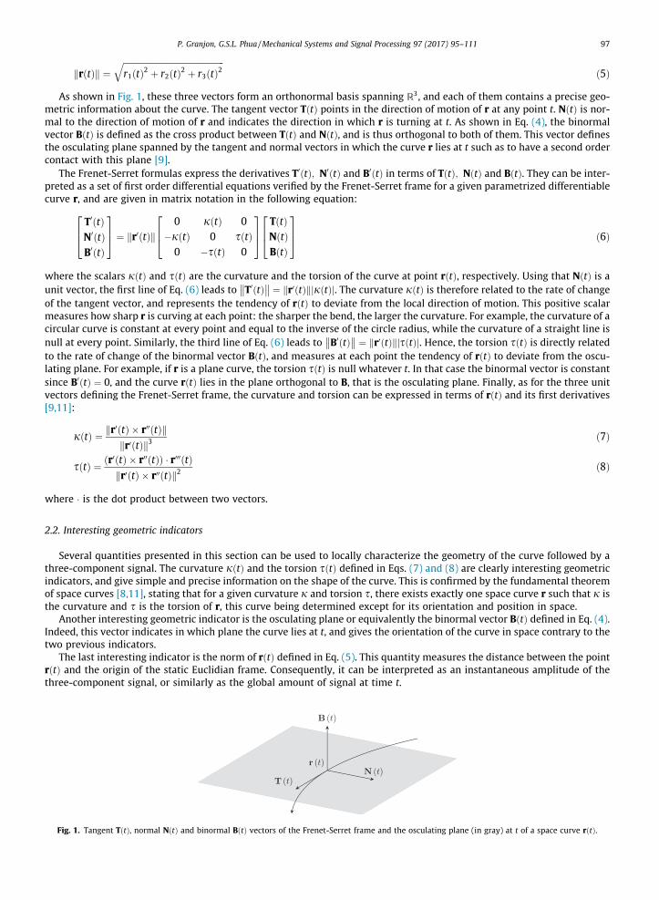
As shown in Fig. 1, these three vectors form an orthonormal basis spanning R3, and each of them contains a precise geo-metric information about the curve. The tangent vector T tð Þ points in the direction of motion of r at any point t. N tð Þ is nor-mal to the direction of motion of r and indicates the direction in which r is turning at t. As shown in Eq. (4), the binormalvector B tð Þ is defined as the cross product between T tð Þ and N tð Þ, and is thus orthogonal to both of them. This vector definesthe osculating plane spanned by the tangent and normal vectors in which the curve r lies at t such as to have a second ordercontact with this plane [9].

The Frenet-Serret formulas express the derivatives T0 tð Þ; N0 tð Þ and B0 tð Þ in terms of T tð Þ; N tð Þ and B tð Þ. They can be inter-preted as a set of first order differential equations verified by the Frenet-Serret frame for a given parametrized differentiablecurve r, and are given in matrix notation in the following equation:

T0 tð ÞN0 tð ÞB0 tð Þ

2

64

3

75 ¼ r0 tð Þk k0 j tð Þ 0

&j tð Þ 0 s tð Þ0 &s tð Þ 0

2

64

3

75T tð ÞN tð ÞB tð Þ

2

64

3

75 ð6Þ

where the scalars j tð Þ and s tð Þ are the curvature and the torsion of the curve at point r tð Þ, respectively. Using that N tð Þ is aunit vector, the first line of Eq. (6) leads to T0 tð Þ

!! !! ¼ r0 tð Þk k j tð Þj j. The curvature j tð Þ is therefore related to the rate of changeof the tangent vector, and represents the tendency of r tð Þ to deviate from the local direction of motion. This positive scalarmeasures how sharp r is curving at each point: the sharper the bend, the larger the curvature. For example, the curvature of acircular curve is constant at every point and equal to the inverse of the circle radius, while the curvature of a straight line isnull at every point. Similarly, the third line of Eq. (6) leads to B0 tð Þ

!! !! ¼ r0 tð Þk k s tð Þj j. Hence, the torsion s tð Þ is directly relatedto the rate of change of the binormal vector B tð Þ, and measures at each point the tendency of r tð Þ to deviate from the oscu-lating plane. For example, if r is a plane curve, the torsion s tð Þ is null whatever t. In that case the binormal vector is constantsince B0 tð Þ ¼ 0, and the curve r tð Þ lies in the plane orthogonal to B, that is the osculating plane. Finally, as for the three unitvectors defining the Frenet-Serret frame, the curvature and torsion can be expressed in terms of r tð Þ and its first derivatives[9,11]:

j tð Þ ¼ r0 tð Þ $ r00 tð Þk kr0 tð Þk k3

ð7Þ

s tð Þ ¼ r0 tð Þ $ r00 tð Þð Þ ' r000 tð Þr0 tð Þ $ r00 tð Þk k2

ð8Þ

where ' is the dot product between two vectors.

2.2. Interesting geometric indicators

Several quantities presented in this section can be used to locally characterize the geometry of the curve followed by athree-component signal. The curvature j tð Þ and the torsion s tð Þ defined in Eqs. (7) and (8) are clearly interesting geometricindicators, and give simple and precise information on the shape of the curve. This is confirmed by the fundamental theoremof space curves [8,11], stating that for a given curvature j and torsion s, there exists exactly one space curve r such that j isthe curvature and s is the torsion of r, this curve being determined except for its orientation and position in space.

Another interesting geometric indicator is the osculating plane or equivalently the binormal vector B tð Þ defined in Eq. (4).Indeed, this vector indicates in which plane the curve lies at t, and gives the orientation of the curve in space contrary to thetwo previous indicators.

The last interesting indicator is the norm of rðtÞ defined in Eq. (5). This quantity measures the distance between the pointr tð Þ and the origin of the static Euclidian frame. Consequently, it can be interpreted as an instantaneous amplitude of thethree-component signal, or similarly as the global amount of signal at time t.

N (t)

B (t)

T (t)

r (t)

Fig. 1. Tangent T tð Þ, normal N tð Þ and binormal B tð Þ vectors of the Frenet-Serret frame and the osculating plane (in gray) at t of a space curve r tð Þ.

P. Granjon, G.S.L. Phua /Mechanical Systems and Signal Processing 97 (2017) 95–111 97

2.3. The case of three-component sinusoidal signals

As previously mentioned, this research work focuses on condition monitoring applications where the measured three-component signals can be considered as quasi-periodic, i.e. as a sum of sine waves. Consequently, it makes sense to studyin detail the geometric characteristics of simple three-component sinusoidal signals by using the different tools presentedin the previous paragraph.

A signal is a three-component sinusoidal signal if each of its components is a sine wave with the same frequency. A three-component sinusoidal signal r can therefore be written mathematically as in Eq. (9), where Ai and ui for i 2 1;2;3f g denotethe amplitude and phase of the sinusoids and f 0 is their frequency.

r tð Þ ¼r1 tð Þr2 tð Þr3 tð Þ

2

64

3

75 ¼A1 sin 2pf 0t þu1ð ÞA2 sin 2pf 0t þu2ð ÞA3 sin 2pf 0t þu3ð Þ

2

64

3

75 ð9Þ

This equation clearly shows that such a signal can be considered as a parametrized differentiable 3D space curve where tis the parameter on which the differential geometric approach presented in the last paragraph can be directly applied.

In this context, it has been demonstrated in [12] that under very general conditions, a three-component sinusoidal signalwith constant amplitudes, phases and frequency follows an elliptical trajectory in a three-dimensional Euclidean frame. Thiselliptical trajectory can be seen as a Lissajous figure in 3D, and is sometimes referred to as a 3D polarization ellipse [13].Using the general expression of three-component sinusoidal signals given in Eq. (9) and the definition of the desired geomet-ric indicators given in Eq. (5), (7), (8), the theoretical expression of the signal norm, curvature and torsion are obtained:

r tð Þk k ¼ffiffiffiffiffiffiffiffiffiffiffiffiffiffiffiffiffiffiffiffiffiffiffiffiffiffiffiffiffiffiffiffiffiffiffiffiffiffiffiffiffiffiffiffiffiffiffiffiffiffiffiffiffiffiffiffiffiffiffiffiffiffiffiffiffiffiffiffiffiffiffiffiffiffiffiffiffiffiffiffiffiffiffiffiffiffiffiffiffiffiffiffiffiffiffiffiffiffiffiffiffiffiffiffiffiffiffiffiffiffiffiffiffiffiffiffiffiffiffiffiffiffiffiffiffiffiffiffiffiffiffiffiffiffiffiffiffiffiffiffiffiA21 sin

2 2pf 0t þu1ð Þ þ A22 sin

2 2pf 0t þu2ð Þ þ A23 sin

2 2pf 0t þu3ð Þq

ð10Þ

j tð Þ ¼

ffiffiffiffiffiffiffiffiffiffiffiffiffiffiffiffiffiffiffiffiffiffiffiffiffiffiffiffiffiffiffiffiffiffiffiffiffiffiffiffiffiffiffiffiffiffiffiffiffiffiffiffiffiffiffiffiffiffiffiffiffiffiffiffiffiffiffiffiffiffiffiffiffiffiffiffiffiffiffiffiffiffiffiffiffiffiffiffiffiffiffiffiffiffiffiffiffiffiffiffiffiffiffiffiffiffiffiffiffiffiffiffiffiffiffiffiffiffiffiffiffiffiffiffiffiffiffiffiffiffiffiffiffiffiffiffiffiffiffiffiffiffiffiffiffiffiffiffiffiffiffiffiffiffiffiA2A3ð Þ2 sin2 u2 &u3ð Þ þ A1A3ð Þ2 sin2 u3 &u1ð Þ þ A1A2ð Þ2 sin2 u1 &u2ð Þ

q

ffiffiffiffiffiffiffiffiffiffiffiffiffiffiffiffiffiffiffiffiffiffiffiffiffiffiffiffiffiffiffiffiffiffiffiffiffiffiffiffiffiffiffiffiffiffiffiffiffiffiffiffiffiffiffiffiffiffiffiffiffiffiffiffiffiffiffiffiffiffiffiffiffiffiffiffiffiffiffiffiffiffiffiffiffiffiffiffiffiffiffiffiffiffiffiffiffiffiffiffiffiffiffiffiffiffiffiffiffiffiffiffiffiffiffiffiffiffiffiffiffiffiffiffiffiffiffiffiffiffiffiffiffiffiffiffiffiffiffiffiffiffiffiffiffiffiffiffiffiffiA21 cos2 2pf 0t þu1ð Þ þ A2

2 cos2 2pf 0t þu2ð Þ þ A23 cos2 2pf 0t þu3ð Þ

# $3r ð11Þ

s tð Þ ¼ 0 ð12Þ

One interesting result is that the torsion is null for such signals, meaning that the corresponding trajectories are asexpected plane curves, with a plane orthogonal to the binormal vector obtained with Eq. (4):

B tð Þ ¼ 1d

A2A3 sin u2 &u3ð ÞA3A1 sin u3 &u1ð ÞA1A2 sin u1 &u2ð Þ

2

64

3

75 ð13Þ

where d ¼ffiffiffiffiffiffiffiffiffiffiffiffiffiffiffiffiffiffiffiffiffiffiffiffiffiffiffiffiffiffiffiffiffiffiffiffiffiffiffiffiffiffiffiffiffiffiffiffiffiffiffiffiffiffiffiffiffiffiffiffiffiffiffiffiffiffiffiffiffiffiffiffiffiffiffiffiffiffiffiffiffiffiffiffiffiffiffiffiffiffiffiffiffiffiffiffiffiffiffiffiffiffiffiffiffiffiffiffiffiffiffiffiffiffiffiffiffiffiffiffiffiffiffiffiffiffiffiffiffiffiffiffiffiffiffiffiffiffiffiffiffiffiffiffiffiffiffiffiffiffiffiffiffiffiffiA2A3ð Þ2 sin2 u2 &u3ð Þ þ A3A1ð Þ2 sin2 u3 &u1ð Þ þ A1A2ð Þ2 sin2 u1 &u2ð Þ

q.

Eqs. (10)–(13) give the theoretical values of the main geometric properties of the space curve corresponding to a three-component sinusoidal signal, and Fig. 2 shows an example of application of these relations for a particular signal. FromFig. 2b and c, it can be seen that the norm and the curvature of r do vary with time t for an ellipse, while the torsion is nullin Fig. 2d and the binormal vector is constant in Fig. 2e as expected. By comparing Fig. 2f and g giving the 3D representationof r and B, it can finally be verified that the binormal vector points in the direction perpendicular to the osculating plane thatthe ellipse is in.

The next section presents a simple algorithm dedicated to the estimation of the geometric properties of interest for three-component signals, and a brief description of its estimation performance in the case of noisy measurements.

3. Estimation algorithm

3.1. General structure

In the last section, the norm r tð Þk k, curvature j tð Þ, torsion s tð Þ and binormal vector B tð Þ have been chosen to characterizethe geometry of the trajectory followed by a three-component sinusoidal signal. Eq. (5), (7), (8) and (4) show that these geo-metric properties can be calculated in terms of the values of the position vector r tð Þ and its first three derivatives withrespect to time t; r0 tð Þ; r00 tð Þ and r000 tð Þ. This remark leads to the three-step algorithm illustrated in Fig. 3, already proposedand detailed in [14,12] to estimate the four previous geometric properties of a three-component signal x at a givenfrequency.

Measured signals usually contain more than one frequency component including noise, and it is therefore essential tofilter such signals first to remove noise and all unwanted frequency components leaving only one frequency component.To carry out this step, a classical linear phase finite impulse response (FIR) frequency-selective filter [15], which can be alowpass, bandpass or highpass filter depending on the value of the selected frequency f 0, is used. This first step producesthe three-component sinusoidal signal r following an elliptical trajectory fromwhich the geometric properties can be further


estimated and analyzed. As can be seen from the mathematical definitions of the four geometric properties of interest, thenext necessary step is the differentiation of r, realized thanks to a simple linear phase FIR differentiator filter. Instead of afull-band differentiator, a partial-band differentiator adapted to the selected frequency f 0 is used in order to avoid amplifyingpossible residual high frequency components and maximize the signal-to-noise ratio (SNR) at the output of each differen-tiator [16]. Since r needs to be differentiated three times, the same differentiator filter is applied three times consecutivelyto r. The use of the frequency-selective and differentiator FIR filters means that there are signal delays that need to be

0.7 0.72 0.74 0.76 0.78 0.8 0.82 0.84 0.86 0.88 0.9 0.92 0.94 0.96 0.98 1−1

01

(a) the three sinusoidal components of r (t)

0.7 0.72 0.74 0.76 0.78 0.8 0.82 0.84 0.86 0.88 0.9 0.92 0.94 0.96 0.98 10

0.51

1.5

(b) ∥r (t)∥

0.7 0.72 0.74 0.76 0.78 0.8 0.82 0.84 0.86 0.88 0.9 0.92 0.94 0.96 0.98 10.5

11.5

2

(c) κ (t)

0.7 0.72 0.74 0.76 0.78 0.8 0.82 0.84 0.86 0.88 0.9 0.92 0.94 0.96 0.98 1−1

−0.50

0.51

(d) τ (t)

0.7 0.72 0.74 0.76 0.78 0.8 0.82 0.84 0.86 0.88 0.9 0.92 0.94 0.96 0.98 1

−0.6−0.4

(e) B (t) in Cartesian coordinates

−10

1−1

01

−1

0

1

r1r2

r 3

(f) r (t) in the 3D Euclidian space

−10

1−1

01

−1

0

1

B1B2

B3

(g) B (t) in the unit sphere

Fig. 2. A three-component sinusoidal signal r tð Þwith f 0 ¼ 10 Hz, A1 ¼ A2 ¼ A3 ¼ 1; u1;u2;u3½ ) ¼ 0; 3p7 ; 8p7% &

, and the theoretical values of its main geometricproperties.


managed after each application of a filter to synchronize the signals. Now that the position vector r and its first three deriva-tives are estimated, the four geometric properties of interest, rk k; j; s and B, can be computed. The third and final step ofthe estimation algorithm illustrated in the block diagram of Fig. 3 is to compute these desired geometric properties using thefour Eqs. (5), (7), (8) and (4), where only basic mathematical operators (division, square root, dot product, cross product) areneeded. Once the geometric properties are computed, their time evolution can be further plotted and analyzed, which isdone in the following section using a synthetic signal.

3.2. Application to a synthetic signal

The proposed algorithm is applied to a synthetic signal including a change in amplitude and phase with the purpose ofillustrating its estimating and tracking capabilities. A three-component sinusoidal signal of frequency f 0 ¼ 10 Hz is first gen-erated with a continuous change in its amplitude (from 20;20;20½ ) to 25;25;25½ )) and phase (from 0; 3p7 ; 8p7

% &to 0; 3p7 ; 5p7

% &)

between 10 s and 10.0625 s. A centered and stationary white Gaussian noise with variance 126 is then added to each sinewave to obtain a noisy three-component sinusoidal signal x, with a global signal-to-noise ratio on each component closeto 2 dB before the change and to 4 dB after the change. The sampling frequency is set to f s ¼ 1024 Hz.

The specifications of the two filters used in the proposed algorithm are set according to the frequency of the sinusoidalcomponents to be characterized. The frequency-selective filter is a bandpass filter with a central frequency equal to the cho-sen frequency f 0 ¼ 10 Hz, a bandwidth of 2 Hz and a transition band of 1 Hz, while the bandwidth of the partial-band dif-ferentiator filter ends at 11 Hz and its stopband starts at 12 Hz. Fig. 4 shows the magnitude of the frequency responsefunction of these two filters, the frequency axis being truncated between 0 and 20 Hz for clarity.

The results obtained by the proposed algorithm applied to the previous synthetic signal are shown in Fig. 5. The noisysignal x is represented in Fig. 5a and the corresponding trajectory in Fig. 5g, where the influence of noise is clearly visible.The bandpass filtered signal r is shown in Fig. 5b and the corresponding trajectory in Fig. 5h, where the noise has been sig-nificantly reduced by the frequency-selective filter. The continuous change in amplitude and phase is visible in these twofigures, where its influence on the shape of the trajectory and therefore on its geometric properties is particularly high-lighted. Fig. 5c–f show the estimated geometric properties where black curves correspond to theoretical values. As expected,r tð Þk k and j tð Þ are time-varying because of the elliptical shape of the trajectory. The variations of these two geometric prop-erties are greater before the change than after, showing that the ellipse of the trajectory followed by r is flatter before thechange than after. Fig. 5e and f show that s and B are approximately constant when amplitudes and phases stay constant.The torsion and binormal vector being related to the osculating plane, this means that the trajectory has a constant osculat-ing plane during these parts of the signal. However, B has different coordinates before and after the change, corresponding to

x (t) frequency-selective

filter

r (t) r (t)

differentiator

differentiator

differentiator

differentiation

r′ (t)

r′′ (t)

r′′′ (t)

equations

(5)

(7)

(8)

(4)

geometric indicators

!∥r (t)∥

!κ (t)

!τ (t)

"B (t)

Fig. 3. Block diagram of the proposed estimation algorithm.

0 2 4 6 8 10 12 14 16 18 200

0.5

1

(a) bandpass filter

0 2 4 6 8 10 12 14 16 18 200

2

4

6

·10−2

(b) differentiator filter

Fig. 4. Frequency response function of the two filters for f 0 ¼ 10 Hz.


two different osculating planes. The theoretical values of these two directions of B are visible in Fig. 5i and drawn as twoblack lines, while the estimated values of B are plotted in red. Finally, the torsion s takes large values only during the changewhere the osculating plane moves, and could be useful as a simple and efficient change detector.

9 9.2 9.4 9.6 9.8 10 10.2 10.4 10.6 10.8 11−50

050

(a) x (t)

9 9.2 9.4 9.6 9.8 10 10.2 10.4 10.6 10.8 11−20

020

(b) r (t)

9 9.2 9.4 9.6 9.8 10 10.2 10.4 10.6 10.8 11

20253035

(c) !∥r (t)∥

9 9.2 9.4 9.6 9.8 10 10.2 10.4 10.6 10.8 110

5 · 10−2

0.1

(d) !κ (t)

9 9.2 9.4 9.6 9.8 10 10.2 10.4 10.6 10.8 11−4−2

024 ·10−3

(e) !τ (t)

9 9.2 9.4 9.6 9.8 10 10.2 10.4 10.6 10.8 11−1

−0.50

0.51

(f) "B (t) in Cartesian coordinates

−500 50

−50050

−500

50

x1x2

x3

(g) x (t) in the 3D Euclidian space

−200 20

−20020

−200

20

r1r2

r 3

(h) r (t) in the 3D Euclidian space

−10

1−1

01

−1

0

1

B1B2

B3

(i) "B (t) in the 3D Euclidian space

Fig. 5. Simulated noisy three-component sinusoidal signal x tð Þ with its main geometric properties.


The performance of the proposed algorithm seems to be good for estimation and tracking the geometric properties ofthree-component sinusoidal signals, although small estimation errors exist. In order to quantify these errors and clarify theirorigin, the influence of different parameters on the estimation performance of this algorithm is detailed in the followingsection.

3.3. Estimation performance

The estimation performance of the proposed algorithm as well as its limits once applied to a three-component sinusoidalsignal are discussed in this section. Three parameters influencing the accuracy of the method have been identified:

* the amount of noise present in the original three-component signal,* the fundamental frequency of the three-component sinusoidal signal to analyze,* the ellipticity of the corresponding three-dimensional trajectory.

Three separate tests are therefore carried out where in each test, two of the parameters remain fixed while the third onevaries within a given range of values. The three-component sinusoidal signal used for these tests is a 40-s discrete-time sig-nal y with a mathematical expression given in Eq. (14).

y ¼A1 sin 2pf 0k=f s þu1ð ÞA2 sin 2pf 0k=f s þu2ð ÞA3 sin 2pf 0k=f s þu3ð Þ

2

64

3

75 where k 2 N ð14Þ

Its sampling frequency f s is 256 Hz and its fundamental frequency is f 0 < 128 Hz. All three sinusoids have the sameamplitude A1 ¼ A2 ¼ A3 ¼ 20 to obtain the same amount of signal whatever the component. The phases u1;u2;u3½ ) areset to obtain a given flatness of the ellipse, measured by the ratio b=a where b is its semiminor axis and a its semimajor axis.In that case, b=a ¼ 0 corresponds to a line segment trajectory and b=a ¼ 1 to a circular trajectory. A centered and stationarywhite Gaussian noise is then added to this pure sinusoidal signal with the same variance whatever the component, theamount of which being measured by the global signal-to-noise ratio SNR computed for one component and expressed indB. The range of values of the different parameters for the three performance tests are summarized in Table 1.

Concerning filters, the frequency-selective filter is a bandpass filter with a central frequency equal to f 0, a bandwidth of2 Hz and a transition band of 1 Hz. The bandwidth of the partial-band differentiator filter ends at f 0 þ 1 Hz and its stopbandstarts at f 0 þ 2 Hz, corresponding to a transition band of 1 Hz.

The estimation performance is measured using the mean squared errors (MSE) of drk k; bB; bj and bs, the estimates of thefour geometric properties of interest rk k; B; j and s. Moreover, in order to facilitate the comparison between the differentcases, the normalized MSE (NMSE) is computed when possible. These quantities are defined in the following equations fordiscrete-time signals where N represents the total number of samples of the signals.

NMSEcrk k¼

PNk¼1 r k½ )k k& dr k½ )k k

# $2

PNk¼1 r k½ )k k2

ð15Þ

NMSEbj ¼

PNk¼1 j k½ ) & dj k½ )

# $2

PNk¼1j k½ )2

ð16Þ

NMSEbB ¼

P3i¼1

1N

XN

k¼1

Bi & dBi k½ )# $2

!

P3i¼1B

2i

¼X3

i¼1

1N

XN

k¼1

Bi & dBi k½ )# $2

!ð17Þ

MSEbs ¼ 1N

XN

k¼1

ds k½ )2 ð18Þ

Eqs. (15) and (16) are used to compute the NMSE of the estimated norm and curvature of the three-component sinusoidalsignal, respectively. Eq. (17) takes into account the three components Bi; i 2 1;2;3½ ) of the binormal vector to compute theglobal NMSE NMSEbB . For three-component sinusoidal signals, B is a constant unit vector as stated in the previous section,

Table 1Range of values of the three parameters for the performance tests.

SNR (dB) f 0 (Hz) b=a

Test 1 0–50 10 0.5994Test 2 20 1–127 0.5994Test 3 20 10 0.0741–1


which explains why the Bi’s are constant andP3

i¼1B2i ¼ 1 in this equation. The MSE of the torsion estimator MSEbs is com-

puted using Eq. (18), where the theoretical value of the torsion s has been set to zero as expected for such signals. This alsoexplains why this error is not normalized.

For each parameter value, averaged MSEs obtained after averaging over 1000 Monte Carlo simulations are computed andanalyzed. The corresponding results are summarized in Fig. 6. Fig. 6a shows these errors with respect to the SNR expressed indB. As expected, the greater the SNR, the smaller the errors, and the linear shape shows that the different MSEs are all inver-sely proportional to the SNR in this range of values. It can be noticed that the worst estimation error is obtained for the cur-vature j. This can be due to the fact that bj is the only estimator that uses derivatives of r and estimates a time-varying

quantity. Indeed, drk k estimates a time-varying quantity without differentiators, while bB and bs need differentiators but esti-mate constant values. Fig. 6b shows the same quantities with respect to the signal frequency f 0 expressed in Hertz. This fig-ure shows that NMSEcrk k

is independent of f 0 while the other MSEs increase when f 0 is very small compared to the sampling

frequency. Contrary todrk k, estimators bB; bj; bs all use derivatives of r, and this decrease in performance is mainly due to theFIR differentiator filters. Indeed, it has been shown in [12] that when the signal frequency f 0 is not much greater than thebandwidth of the bandpass filter, each differentiation step decreases the SNR because of the residual noise left by the band-pass filter, and finally deteriorates the global estimation performance of the algorithm. Fig. 6c shows the influence of theellipticity b=a on the estimation errors. Concerning NMSEbj , Eq. (7) shows that the denominator of the curvature j tð Þ is

r0 tð Þk k3. Now, the flatter the ellipse, the faster r0 tð Þk k3 tends to zero at the tips of the ellipse, and as r0 tð Þk k tends to zero,j tð Þ becomes infinite and so does NMSEbj . In the worst-case scenario, the trajectory is a line segment, the flattest ellipse pos-sible where r0 tð Þk k ¼ 0 at the tips where the curvature is impossible to estimate in this case. Concerning the estimation errorsof the binormal vector NMSEbB and of the torsion MSEbs , they both increase the flatter the ellipse. When the ellipse is flatter, it

tends to a line segment trajectory for which the osculating plane, the binormal vector and the torsion are not correctlydefined. Therefore, it is not surprising that these quantities are difficult to estimate when the elliptical trajectory followedby the position vector flattens increasingly.

From these performance tests, several things should be kept in mind before applying this algorithm to experimental sig-nals. A lot of noise in the measured signal deteriorates the estimation performance of the algorithm, especially when the sig-nal frequency is not greater than the bandwidth of the frequency-selective filter. Moreover, if the signal follows a trajectorythat is almost a line or a very flat ellipse, this algorithm will produce higher estimation errors.

4. Bearing faults monitoring with three-axis vibration signals

In this section, the proposed algorithm is applied to vibration signals for bearing faults detection in rotating machines.The objective is to extract bearing fault indicators from the geometric characteristics of the trajectory followed by vibrationsignals measured in three orthogonal directions.

4.1. Experimental setup and datasets

The signals used in this section are measured on the test bench represented in Fig. 7. The kinematic chain consists in alow-speed shaft, a multiplier gearbox and a high-speed shaft. The output load is an induction generator and the operatingconditions are determined by controlling the speed of the low-speed shaft thanks to a geared motor. This bench can be used

0 10 20 30 40 50

normcurvaturebinormaltorsion

(a) test 1: errors versus SNR20 40 60 80 100 120

10-11

10-9

10-7

10-5

10-3

10-1

10-11

10-9

10-7

10-5

10-3

10-1

10-11

10-9

10-7

10-5

10-3

10-1


(b) test 2: errors versus f0

0.1 0.2 0.3 0.4 0.5 0.6 0.7 0.8 0.9 1


(c) test 3: errors versus b/a

Fig. 6. Averaged estimation errors NMSEcrk k; NMSEbj ; NMSEbB and MSEbs obtained for the three performance tests.


to emulate the structure and behavior of a geared wind turbine, but also of an industrial system if the output generator isconsidered as a mechanical load. Loading unit 1 mounted on the low-speed shaft is used to accelerate the deterioration of themain bearing by applying radial and axial load to this component. The type of bearing used in the test is a radial sphericalroller bearing with an inside diameter of 50 mm, on which natural faults may appear on any part, be it the inner race, outerrace, bearing balls or cage.

Several consecutive endurance tests were conducted with an alternation of degradation phases and measurement phasesfor which the rotational speed of the low-speed shaft was kept constant at 20 rpm. At the end of each test, the bearing wasdamaged up to an unknown degradation level and dismounted to visually characterize the level of damage. The period oftime covered by this study starts on October 7 2013 and ends on January 31 2014. During this period, a natural faultappeared on November 8, the corresponding measurements were stopped on November 19, the faulty bearing was replacedwith a new one on December 16 and a new measurement process started on December 17. Table 2 summarizes these eventswith the corresponding dates. Fig. 8 shows the state of the bearing at the end of the test used in this work, where localizedspalling on the outer race is clearly visible.

The data measured on this test bench and used in this work are vibration signals measured using three mono-axialaccelerometers mounted on ‘‘loading unit 1” in three orthogonal directions in order to obtain the vibrations in the threedirections of 3D Euclidean space. 20 datasets obtained between October 7 2013 and January 31 2014 are used. Each datasetconsists in a three-component vibration signal of 1500 samples acquired with a sampling frequency of 100 Hz.

4.2. Experimental results

First of all, the presence of the outer race fault during the test can be verified thanks to the power spectral density (PSD) ofeach component of the three-axis vibration signals before and after the fault appears. Indeed, bearings faults generatemechanical impacts and consequently vibrations with a frequency depending on the geometric characteristics of the bearing,the rotating speed of the shaft where the bearing is mounted on, and the type and location of the fault in the bearing. In thisexperiment, the expected outer race fault frequency of 2.72 Hz is clearly visible in Fig. 9 showing the PSD of each component

Fig. 7. Structure of the test bench used for bearing faults monitoring [17].

Table 2Main events and dates during the endurance tests of interest.

Date Event

October 7 2013 Start of the 1st testNovember 8 2013 Fault appearsNovember 19 2013 End of the 1st testDecember 16 2013 Main bearing is replacedDecember 17 2013 Start of the 2nd test


for two datasets: in blue, the PSD of dataset November 7 2013 (before the fault appears), and in orange the PSD of datasetNovember 19 2013 (after the fault appears). This result confirms the presence of this particular fault in the monitored bear-ing before its visual inspection.

Next, the algorithm detailed in the previous section is applied to each dataset in order to estimate the time evolution ofthe four geometric properties of interest at different dates all along the test, and to analyze their behavior regarding the pres-ence of the fault. Figs. 10 and 11 show the results obtained for the two same datasets as previously: dataset November 72013 before the fault appears, and dataset November 19 2013 after the fault appears. These figures show vibration signalsbefore and after frequency-selective filtering as well as the four geometric properties estimated by the algorithm. Figs. 10a, gand 11a, g show that without the frequency-selective filter (a bandpass filter with a central frequency set to the fault fre-quency 2.72 Hz), no meaningful geometric information can be extracted from the data due to the presence of wide-bandnoise and several sinusoidal components. The signal r tð Þ obtained after this necessary filtering step in shown in Figs. 10b,

(a) outer race defects (b) detail of the largest defect

Fig. 8. Spalling on the outer race of the bearing (courtesy of CETIM).

1.6 1.8 2 2.2 2.4 2.6 2.8 3 3.2 3.4 3.6 3.8 4

frequency (Hz)

1.6 1.8 2 2.2 2.4 2.6 2.8 3 3.2 3.4 3.6 3.8 4

frequency (Hz)

1.6 1.8 2 2.2 2.4 2.6 2.8 3 3.2 3.4 3.6 3.8 4

frequency (Hz)

dB

(a) 1st component

dB

(b) 2d component

−100−80−60−40

−100−80−60−40

−100−80−60−40

dB

(c) 3rd component

Fig. 9. Power spectral density of the three-axis vibration signal before (in blue) and after (in orange) the fault appeared. (For interpretation of the referencesto color in this figure legend, the reader is referred to the web version of this article.)


h and 11b, h. Before the fault appears, its 3D trajectory is completely unstructured in Fig. 10b and h, while a typical ellipticaltrajectory is clear in Fig. 11b and h once the fault appears. This remark is confirmed by the four geometric propertiesobtained for the two datasets. The signal norm in Figs. 10c and 11c show that r tð Þk k increases in amplitude in case of a fault,

20 20.5 21 21.5 22 22.5 23 23.5 24 24.5 25−4−2

024

·10−3

(a) x (t)

20 20.5 21 21.5 22 22.5 23 23.5 24 24.5 25−1

−0.50

0.51 ·10−3

(b) r (t)

20 20.5 21 21.5 22 22.5 23 23.5 24 24.5 250

0.5

1·10−3

(c) !∥r (t)∥

20 20.5 21 21.5 22 22.5 23 23.5 24 24.5 250

2,0004,0006,000

(d) !κ (t)

20 20.5 21 21.5 22 22.5 23 23.5 24 24.5 25−1,000

−5000

5001,000

(e) !τ (t)

20 20.5 21 21.5 22 22.5 23 23.5 24 24.5 25−1

−0.50

0.51


−50

5

·10−3−50

5

·10−3

−5

0

5·10−3

x1x2

x3

(g)x (t) in the 3D Euclidian space

−10

1

·10−3−10

1

·10−3

−1

0

1·10−3

r1r2

r 3


−10

1−1

01

−1

0

1

B1B2

B3


Fig. 10. Three-axis vibration signal before the bearing fault appears with its main geometric properties.


because the amount of signal at the fault frequency increases as the fault appears. Notice also that r tð Þk k has a more regularpattern after the fault appears, corresponding to a more structured 3D trajectory. The second geometric property, the cur-vature j tð Þ shown in Figs. 10d and 11d, behaves inversely. Before the fault appears, j tð Þ takes very large values and seems

20 20.5 21 21.5 22 22.5 23 23.5 24 24.5 25−4−2

024

·10−3

(a) x (t)

20 20.5 21 21.5 22 22.5 23 23.5 24 24.5 25−1

−0.50

0.51 ·10−3

(b) r (t)

20 20.5 21 21.5 22 22.5 23 23.5 24 24.5 250

0.5

1·10−3

(c) !∥r (t)∥

20 20.5 21 21.5 22 22.5 23 23.5 24 24.5 250

2,0004,0006,000

(d) !κ (t)

20 20.5 21 21.5 22 22.5 23 23.5 24 24.5 25−1,000

−5000

5001,000

(e) !τ (t)

20 20.5 21 21.5 22 22.5 23 23.5 24 24.5 25−1

−0.50

0.51


−50

5

·10−3−50

5

·10−3

−5

0

5·10−3

x1x2

x3


−10

1

·10−3−10

1

·10−3

−1

0

1·10−3

r1r2

r 3


−10

1−1

01

−1

0

1

B1B2

B3


Fig. 11. Three-axis vibration signal after the bearing fault appears with its main geometric properties.


to fluctuate randomly, which represents a completely unstructured trajectory. When the fault appears, j tð Þ decreases andoscillates regularly around smaller values, which is expected since the 3D trajectory becomes more structured and ellipticalin that case. The third geometric property, the torsion, is closely related to the variations of the binormal vector. As can beseen in Fig. 10e, the torsion s tð Þ reflects the frequent and big changes in the binormal vector B tð Þ, highlighting an unstruc-tured shape for the trajectory. However, in Fig. 11e, s tð Þ takes smaller values, corresponding to a more steady trajectoryplane. The fourth and last geometric property is the binormal vector B tð Þ shown in Figs. 10f, i and 11f, i. From these figures,it can be seen that before the fault appears, B tð Þ does not point in a particular direction and varies randomly all along themeasurement. Once the fault appears, it points in a stable direction, orthogonal to the plane that the 3D trajectory of r tð Þis in. Finally, the results obtained before the fault appears and represented in Fig. 10 can be summarized as follows:r tð Þk k shows that there is no significant signal at the fault frequency while j tð Þ; s tð Þ and B tð Þ show that the corresponding3D trajectory has no structured shape. On the contrary, once the fault appears, the same quantities represented in Fig. 11lead to the opposite conclusion: r tð Þk k indicates that there is a significant component at the fault frequency and j tð Þ; s tð Þand B tð Þ indicate that the resulting trajectory has a structured elliptical shape with almost constant characteristics.

Different bearing fault indicators can be proposed using the previous results, and several have been studied in [12]. Oneparticularly interesting indicator quantifying the variations of the binormal vector is its standard deviation, defined has thesquare root of the sum of the variances of each of its components. As seen through the previous experimental results, thisvector is nearly constant in the faulty case and varies strongly and randomly in the healthy case. Therefore, its standard devi-ation should be close to zero in the faulty case and should take large values in the healthy case. This is verified in Fig. 12where this quantity has been computed for each dataset measured during the endurance test, and where the two verticalred lines mark when the bearing defect appears and when the faulty bearing is replaced by a new one. Another interestingproperty clearly visible in this figure is that this indicator is bounded between 0 and 1. This maximal value is due to the factthat the binormal vector is a unit vector with components bounded between +1. Indeed, before the fault appears, the cor-responding 3D trajectory is unstructured and there is no preferred direction pointed to by the binormal vector as illustratedin Fig. 10f and i. In that case, the binormal vector can be thought of as a random variable with each of its components fol-lowing a uniform probability distribution between +1. Their variance is therefore equal to 1=3 and the standard deviation ofB tð Þ previously defined is then equals to 1. On the contrary, when a fault occurs, the binormal vector is nearly constant andits standard deviation stays close to zero. These experimental results show that the type of information provided by the geo-metric properties of interest are different in nature and complementary. The signal norm r tð Þk k is connected to the amount ofsignal at the fault frequency as well as to the shape of the trajectory. The curvature j tð Þ gives information about the shape ofthe trajectory, such as the flatness of the ellipse. The binormal vector B tð Þ gives the plane the trajectory is in, whereas thetorsion s tð Þ shows when this plane changes. These geometric informations can be used to deeply characterize the detectedfaults, but they can also be used to detect the presence of a fault in the monitored bearing as shown at the end of this section.

The next section presents a different experimental application of these tools.

5. Voltage dips monitoring with three-phase voltage signals

This section concerns the application of the proposed algorithm to the monitoring of voltage dips in three-phase powernetworks. These phenomena are the most common type of power-quality disturbances, and lead to important economiclosses and distorted quality of industrial products [18]. Thus, voltage dips monitoring has become an essential requirementfor power quality monitoring in power networks, and several methods have been developed to detect and characterize suchdisturbances [19,20]. However, most of these techniques consider three-phase measurements as three separate one-dimensional quantities, and process each phase voltage independently from each other. In [7], a first step is taken wherethe three-phase quantities are considered two-dimensional after a Clarke transform [21], and are processed as complex-valued signals. In this section, the proposed method is applied in order to consider the three-phase voltages as a singlethree-dimensional quantity. The objective, if not to obtain better results than previously proposed methods, is to adopt adifferent and complementary point of view by considering three-phase voltages as a whole and gain additional informationin the process.

The proposed algorithm is applied to an experimental three-phase voltage signal x tð Þ with a fundamental frequencyf 0 ¼ 50 Hz and sampled at f s ¼ 3200 Hz. This data, measured at one point of a high-voltage power network, is representedin Fig. 13a. It clearly undergoes a voltage dip between t ¼ 50 ms and t ¼ 120 ms with the dip being more pronounced for the

Oct13 Nov13 Dec13 Jan14 Feb140

0.5

1

Fig. 12. Standard deviation of the binormal vector obtained for each dataset during the endurance test (left red line: bearing defect appears, right red line:bearing replaced). (For interpretation of the references to color in this figure legend, the reader is referred to the web version of this article.)


blue voltage. The corresponding three-dimensional trajectory is shown in Fig. 13g, where a change in the trajectory can alsobe seen. Voltage signals measured in power networks are very specific, and mostly consist in one large sine wave called thefundamental component, added to smaller harmonics, the closest and most significant being the 5th and 7th [18]. This

0 20 40 60 80 100 120 140 160 180 200 220 240−2−1

012 ·104

(a) x (t)

0 20 40 60 80 100 120 140 160 180 200 220 240−2−1

012 ·104

(b) r (t)

0 20 40 60 80 100 120 140 160 180 200 220 2401

1.5

2·104

(c) !∥r (t)∥

0 20 40 60 80 100 120 140 160 180 200 220 2400.5

11.5

·10−4

(d) !κ (t)

0 20 40 60 80 100 120 140 160 180 200 220 240−1

012 ·10−5

(e) !τ (t)

0 20 40 60 80 100 120 140 160 180 200 220 2400.4

0.6

0.8


−20

2

·104−20

2

·104

−2

0

2·104

x1x2

x3


−20

2

·104−20

2

·104

−2

0

2·104

r1r2

r 3


−10

1−1

01

−1

0

1

B1B2

B3


Fig. 13. Experimental three-phase voltage signal x tð Þ containing a voltage dip with its main geometric properties (time t in ms).


particularity can be used to simplify the first step of the proposed algorithm. Instead of a bandpass filter, a simple lowpassfilter is sufficient to separate the fundamental component from the others and obtain the desired three-component sinu-soidal signal r tð Þ. Since the fundamental frequency is 50 Hz, the passband of the lowpass filter is set to 60 Hz and its tran-sition band to 200 Hz. Similarly, the passband of the differentiator filter ends at 60 Hz and its stopband starts at 260 Hz. Thecorresponding position vector r tð Þ, shown in Fig. 13b, is then obtained at the output of the lowpass filter, and is representedas a moving point in 3D Euclidean space in Fig. 13h. These figures show that r tð Þ rotates around the origin with frequencyf 0 ¼ 50 Hz, and that the three-dimensional trajectory followed by r tð Þ changes during the measurement – clearly there aretwo different osculating planes – due to the voltage dip.

Next, the four geometric properties of r tð Þ are estimated using the proposed algorithm. The estimated signal norm, cur-vature, torsion and binormal vector are shown in Fig. 13c–f respectively. Notice that the torsion takes significant values onlyat the beginning and at the end of the voltage dip. Apart from these special periods of time, the torsion remains small andclose to zero. Geometrically, this means that the 3D trajectory followed by r tð Þ stays in a fixed plane, except at these specificperiods of time during which the osculating plane changes significantly. Notice also that the osculating plane containing thetrajectory during and outside the voltage dip is not the same. This is confirmed by changes in the binormal vector: its Carte-sian coordinates plotted in Fig. 13f clearly take different values during and outside the voltage dip, which is confirmed by its3D representation in Fig. 13i. The curvature provides a different kind of information, related to the shape of the trajectoryfollowed by r tð Þ. Outside the voltage dip, the curvature is nearly constant so the trajectory is circular, which is what the tra-jectory of a balanced three-phase voltage should be. Indeed, a balanced three-phase voltage v can be written in the form of

Eq. (19), corresponding to a circular trajectory of radiusffiffi32

qV and thus of constant curvature.

v tð Þ ¼V cos 2pf 0t þuð Þ

V cos 2pf 0t þu& 2p3

' (

V cos 2pf 0t þu& 4p3

' (

2

64

3

75 ð19Þ

During the dip, the curvature varies with frequency 2f 0 ¼ 100 Hz, i.e. twice per revolution. When the curvature in Fig. 13dis compared to the signal norm in Fig. 13c, it is clear that when r tð Þ is close to the origin, the curvature is small and vice versa.This corresponds to a trajectory with an elliptical shape. Therefore, the curvature shows that the trajectory of r tð Þ changesfrom a circle outside the dip to an ellipse during the dip.

The results obtained through this experimental data set show that geometric properties lead to important geometricinformation concerning the three-dimensional trajectory followed by r tð Þ and through this, provide information about thestate of the corresponding three-phase system. In other words, the proposed algorithm can be used to analyze the geometricchanges in the trajectory of three-phase voltages as well as to detect and also possibly characterize voltage dips. More specif-ically, the torsion s can be used for dip detection as it only takes significant values when there is a change in the osculatingplane, indicating that there is a change in the system. The detected dips can then be characterized thanks to the osculatingplane given by the coordinates of the binormal vector B. Along with the signal norm rk k and the curvature j, this leads toinformation about the shape of the trajectory during the dips.

6. Conclusions

With the objective of condition monitoring, this article proposes a method of estimating the geometric properties of thetrajectory followed by a three-component sinusoidal signal in three-dimensional Euclidean space, along with a simple andefficient estimation algorithm. The proposed method is applied to two types of experimental data: three-axis vibration sig-nals measured on a rotating machine and used for bearing fault monitoring, and voltage signals measured on a three-phasepower network and used for voltage dips monitoring. The estimated geometric properties of the three-dimensional ellipticaltrajectory followed by these signals reflect the bearing faults and the voltage dips to be detected. From these results, it can beconcluded that the proposed method is useful as it gives different and complementary information to existing conditionmonitoring methods.

Several improvements to the method can be considered in future works. The noise removal and frequency selection stepcan be further developed and improved so that the noise is removed more precisely and the frequency component is isolatedmore accurately. Certain geometric properties such as the semimajor axis, semiminor axis as well as the orientation in spaceof the obtained ellipse can be estimated in order to complete the geometric information given by the algorithm. In addition,the proposed method could be extended to more complex deterministic signals such as periodic signals containing morethan a single sinusoidal component and even further, to random signals. It can also be noticed that the geometric approachrelying on Frenet-Serret frame and formulas have been generalized to signals with any number of components [22,23]. Thisallows to consider the application of the proposed method to signals with a number of components higher than three, even ifin this case the geometric meaning of the obtained indicators is not so simple to analyze.

Concerning applications, the results already obtained for voltage dips and bearing faults detection could be taken a stepfurther. More particularly, the estimated geometric properties could by used to classify the detected voltage dips or deeplycharacterize the detected bearing fault. Indeed, the geometric properties of vibration signals are directly connected to thethree-dimensional movements of the rotating machine they are measured from, and thus have clear physical significations.


For example the main direction of vibration, which is reflected thanks to the binormal vector defining the plane of the ellip-tical trajectory, can be used to deduce the direction in which the bearing is vibrating.

Acknowledgments

The authors would like to thank CETIM (Centre Technique des Industries Mécaniques) for providing the test-bench andexperimental data.

References

[1] D.R. Brillinger, Time Series: Data Analysis and Theory, Society for Industrial and Applied Mathematics (SIAM), 2001.[2] P. Granjon, Complex-valued signal processing for condition monitoring, in: Fifth International Conference on Condition Monitoring and Machinery

Failure Prevention Technologies, Edinburgh, United Kingdom, 2008.[3] P.J. Schreier, L.L. Scharf, Statistical Signal Processing of Complex-Valued Data: The Theory of Improper and Noncircular Signals, Cambridge University

Press, 2010.[4] N. Bachschmid, P. Pennacchi, A. Vania, Diagnostic significance of orbit shape analysis and its application to improve machine faults detection, J. Braz.

Soc. Mech. Sci. Eng. 26 (2) (2004) 200–208.[5] C.W. Lee, Y.S. Han, The directional Wigner distribution and its applications, J. Sound Vib. 216 (4) (1998) 585–600.[6] Y.S. Han, C.W. Lee, Directional Wigner distribution for order analysis in rotating/reciprocating machine, Mech. Syst. Signal Process. 13 (5) (1999) 723–

737.[7] V. Ignatova, P. Granjon, S. Bacha, Space vector method for voltage dips and swells analysis, IEEE Trans. Power Deliv. 24 (4) (2009) 2054–2061.[8] M.P. do Carmo, Differential Geometry of Curves and Surfaces, Prentice Hall, 1976.[9] B. O’Neill, Elementary Differential Geometry, Academic Press, 1966.[10] E. Cartan, La théorie des groupes finis et continus et la géométrie différentielle, traitées par la méthode du repère mobile, Gauthier-Villars, 1937.[11] M. Spivak, A Comprehensive Introduction to Differential Geometry, second ed., vol. 2, Publish or Perish, 1979.[12] G.S.-L. Phua, Estimation of Geometric Properties of Three-Component Signals for Condition Monitoring, Theses, Université Grenoble Alpes, January

2016. <https://tel.archives-ouvertes.fr/tel-01295193>.[13] E. Wolf, Introduction to the Theory of Coherence and Polarization of Light, Cambridge University Press, 2007.[14] G. Phua, P. Granjon, Estimation of geometric properties of three-component sinusoidal signals for system monitoring, in: The 7th International

Conference on Acoustical and Vibration Methods Development and Applications for Surveillance and Diagnostics (Surveillance 7), 2013.[15] J.G. Proakis, D.G. Manolakis, Digital Signal Processing: Principles, Algorithms, and Applications, fourth ed., Pearson Education, 2007.[16] C.-C. Tseng, S.-L. Lee, Linear phase FIR differentiator design based on maximum signal-to-noise ratio criterion, Signal Process. 86 (2) (2006) 388–398.[17] N. Bédouin, S. Sieg-Zieba, Endurance testing on a wind turbine test bench: a focus on slow rotating bearing monitoring, in: Twelfth International

Conference on Condition Monitoring and Machinery Failure Prevention Technologies, Oxford, United Kingdom, 2015.[18] M.H.J. Bollen, Understanding Power Quality Problems: Voltage Sags and Interruptions, Wiley-IEEE Press, 2000.[19] M.H.J. Bollen, I.Y.H. Gu, Signal Processing of Power Quality Disturbances, Wiley-IEEE Press, 2006.[20] M.H.J. Bollen, L.D. Zhang, Different methods for classification of three-phase unbalanced voltage dips due to faults, Electric Power Syst. Res. 66 (1)

(2003) 59–69.[21] J.M. Aller, A. Bueno, T. Paga, Power system analysis using space-vector transformation, IEEE Trans. Power Syst. 17 (4) (2002) 957–965.[22] C. Jordan, Sur la théorie des courbes dans l’espace à n dimensions, Compt.-Rend. l’Acad. Sci. 79 (1874) 795–797.[23] P. Griffiths, On Cartan’s method of lie groups and moving frames as applied to uniqueness and existence questions in differential geometry, Duke Math.

J. 4 (1974) 775–814.


http://refhub.elsevier.com/S0888-3270(17)30186-3/h0005



















https://tel.archives-ouvertes.fr/tel-01295193
















mechanical systems and signal processing - gipsa-lab.frpierre.granjon/doc/publi/artmssp17b.pdf ·...

Documents