Guo, Z., Shi, X., Chen, Y., Chen, H., Peng, X., and Harrison, P. (2014) Mechanical modeling of incompressible particle-reinforced neo-Hookean composites based on numerical homogenization. Mechanics of Materials, 70 . pp. 1-17. ISSN 0167-6636 Copyright © 2014 Elsevier Ltd. http://eprints.gla.ac.uk/89714 Deposited on: 18 February 2014

Enlighten – Research publications by members of the University of Glasgow

http://eprints.gla.ac.uk

Mechanics of Materials 70 (2014) 1–17

Contents lists available at ScienceDirect

Mechanics of Materials

journal homepage: www.elsevier .com/locate /mechmat

Mechanical modeling of incompressible particle-reinforcedneo-Hookean composites based on numerical homogenization

http://dx.doi.org/10.1016/j.mechmat.2013.11.0040167-6636/� 2013 Elsevier Ltd.This is an open access article under the CC BY license (http://creativecommons.org/licenses/by/3.0/).

⇑ Corresponding authors. Address: State Key Laboratory of Coal MineDisaster Dynamics and Control, Chongqing University, Chongqing400044, China. Tel.: +86 13983897097 (Z. Guo).

E-mail addresses: zyguo01@gmail.com (Z. Guo), xqpeng@sjtu.edu.cn(X. Peng).

Zaoyang Guo a,b,⇑, Xiaohao Shi c, Yang Chen b, Huapeng Chen d, Xiongqi Peng e,⇑,Philip Harrison f

a State Key Laboratory of Coal Mine Disaster Dynamics and Control, Chongqing University, Chongqing 400044, Chinab Department of Engineering Mechanics, Chongqing University, Chongqing 400044, Chinac Institute of Biomedical Engineering and Health Sciences, Changzhou University, Changzhou, Jiangsu 213164, Chinad School of Engineering, University of Greenwich, Chatham Maritime, Kent ME4 4TB, UKe Department of Plasticity Technology, Shanghai Jiao Tong University, Shanghai 200030, Chinaf School of Engineering, University of Glasgow, Glasgow G12 8QQ, UK

a r t i c l e i n f o a b s t r a c t

Article history:Received 1 May 2013Received in revised form 6 October 2013Available online 4 December 2013

Keywords:Particle-reinforced compositeRepresentative volume element (RVE)Neo-HookeanNumerical homogenizationHyperelasticity

In this paper, the mechanical response of incompressible particle-reinforced neo-Hookeancomposites (IPRNC) under general finite deformations is investigated numerically. Three-dimensional Representative Volume Element (RVE) models containing 27 non-overlappingidentical randomly distributed spheres are created to represent neo-Hookean compositesconsisting of incompressible neo-Hookean elastomeric spheres embedded within anotherincompressible neo-Hookean elastomeric matrix. Four types of finite deformation (i.e., uni-axial tension, uniaxial compression, simple shear and general biaxial deformation) are sim-ulated using the finite element method (FEM) and the RVE models with periodic boundarycondition (PBC) enforced. The simulation results show that the overall mechanicalresponse of the IPRNC can be well-predicted by another simple incompressible neo-Hook-ean model up to the deformation the FEM simulation can reach. It is also shown that theeffective shear modulus of the IPRNC can be well-predicted as a function of both particlevolume fraction and particle/matrix stiffness ratio, using the classical linear elastic estima-tion within the limit of current FEM software.

� 2013 Elsevier Ltd. This is an open access article under the CC BY license (http://creati-vecommons.org/licenses/by/3.0/).

1. Introduction polynomial to predict the small strain Young’s modulus

A fundamental problem for particle-reinforced compos-ites (PRC) is to predict the overall mechanical behavior ofthe composite based on the mechanical properties of theconstituents and the microstructure of the composites.Guth (1945) extended Einstein’s linear estimate originallydeveloped for viscous fluid and proposed a second order

of (rigid) particle-filled solids. Kerner (1956) designed anaveraging procedure to estimate the effective shear modu-lus and bulk modulus of the PRC. Hill (1965) proposed aself-consistent model to estimate the effective shear mod-ulus of the PRC. The three-phase model developed byChristensen and Lo (1979) gives a very good prediction ofthe PRCs effective shear modulus (Segurado and Llorca,2002). Torquato (1998) derived accurate expressions forthe bulk and shear moduli of the PRC based on a third-or-der approximation. Although a few studies investigatedsome special microstructures such as cubic arrays ofspheres (e.g., Cohen, 2004), most papers in the literaturehave focused on macroscopically isotropic composites

2 Z. Guo et al. / Mechanics of Materials 70 (2014) 1–17

with randomly distributed particles. Besides the directestimation of the effective moduli of the PRC, some rigor-ous bounds for the elastic properties of the PRC have beenobtained from variational principles (e.g., Hashin andShtrikman, 1963). Another approach to investigate the‘‘overall’’ mechanical behavior of the PRC is to solve theboundary value problems for a representative volume ele-ment (RVE) model of the composite numerically (Michelet al., 1999). Drugan and Willis (1996) showed that a smallsize RVE model can predict accurately the mechanical re-sponse of the PRC. Segurado and Llorca (2002) provided acomprehensive numerical study of the mechanical proper-ties of the linear elastic PRC using multi-particle RVEmodels.

Although the mechanical properties of the PRC in infin-itesimal strain have been investigated extensively, theirmechanical behavior in the finite deformation regime isstill not well-understood due to the intrinsic difficulties re-lated to the geometrical and material nonlinearities. Hill(1972) proposed a set of macroscopic variables for consti-tutive modeling of composites in finite deformation. Basedon that, Ogden (1974) derived an approximate expressionfor the overall bulk modulus of the PRC with second-orderisotropic compressible elastic constituents under finitestrain. Hashin (1985) studied the response of hyperelasticPRC under hydrostatic loading. Imam et al. (1995) derivedthe second order elastic field for incompressible hyperelas-tic composites with dilute inclusions, which was then em-ployed to estimate the overall moduli of the PRC. Althoughrecently several research groups have investigated hyper-elastic composites with inclusions in two dimension(which physically implies composites with aligned fiberreinforcement) and some related boundary value problemsare solved analytically (e.g., deBotton et al., 2006; Guoet al., 2008; Guo et al., 2006; Lopez-Pamies, 2010), analyt-ical solutions for three-dimensional PRC model under gen-eral homogeneous displacement boundary conditions arefar more difficult. Castaneda (1989) proposed a self-consis-tent approach to predict the shear modulus of incompress-ible particle-reinforced neo-Hookean composites (IPRNC).Bergstrom and Boyce (1999) used the concept of strainamplification under large strain to estimate the shear mod-ulus of incompressible neo-Hookean composites filledwith rigid particles. Because these two models are notbased on an accurate approximation of the elastic fields,it is not surprising to find that they don’t provide good esti-mates of effective shear modulus of IPRNC with moderateparticle volume fractions. Recently Avazmohammadi andCastaneda (2012) developed a tangent second-order(TSO) method to investigate the macroscopic response ofPRC in finite deformation and an explicit formula is derivedto approximate the strain energy of incompressible neo-Hookean composites reinforced with rigid particles.

The numerical studies of hyperelastic composites avail-able in the literature are also mainly limited to two-dimensional problems of composites with aligned fibersor voids (e.g., Guo et al., 2008; Moraleda et al., 2007,2009; Tang et al., 2012a, b), though Bergstrom and Boyce(1999) used simple 2D axisymmetric models to simulateIPRNC under uniaxial deformation. Three-dimensionalRVE modeling in finite deformation is only investigated

for single-fiber unit cell (Guo et al., 2007). To the best ofthe authors’ knowledge, there is no comprehensive numer-ical study of the PRC under finite deformation published inthe literature.

Because it is difficult to predict the mechanical responseof the PRC under general finite deformation theoreticallydue to the related geometrical and material nonlinearities,this study employs the numerical homogenization ap-proach to investigate the mechanical behavior of the sim-plest hyperelastic PRC under general finite deformation,in which the mechanical properties of both the matrixand the reinforcement are described by an incompressibleneo-Hookean model respectively. In this paper, three-dimensional RVE models are created to represent the neo-Hookean composite which consists of one incompressibleneo-Hookean elastomer embedded with another randomlydistributed equal-sized spherical incompressible neo-Hookean particle reinforcement. Commercial finite ele-ment analysis software ABAQUS is employed for thenumerical simulations of the RVE models. Periodic bound-ary conditions (PBC) are implemented in the RVE modelswhen general finite deformation is applied to the RVE mod-els. The numerical results show that the overall mechanicalresponses of the IPRNC can be well predicted by anothersimple incompressible neo-Hookean model. The simulationresults also suggest that the classical linear elastic estima-tion (Christensen and Lo, 1979) can be used to predict theeffective shear modulus of the IPRNC with different particlevolume fraction and different particle/matrix stiffness ratio.

The structure of the paper is as follows: In Section 2, theIPRNC to be investigated is described and the theoreticalbasis of the numerical homogenization in finite deforma-tion (Hill, 1972; Ogden, 1974) is also introduced. In Section3, the RVE models are developed for numerical simulationsusing finite element method (FEM) and some related issues(e.g., isotropy of the RVE models, FEM mesh) are discussed.The results of the RVE simulations are presented and inves-tigated in Section 4. The effective modulus of the hyper-elastic composites is also compared with classical linearelastic estimation. Some concluding remarks are given inSection 5.

2. Particle-reinforced neo-Hookean composites andtheoretical basis of numerical homogenization

First of all, some basic concepts in continuum mechan-ics need to be introduced. For a continuum solid, the defor-mation gradient is defined as F ¼ @x=@X, where X and xdenote the positions of a typical material point respec-tively in the original (undeformed) and deformed configu-ration of the solid, respectively. The mechanical behaviorof an isotropic hyperelastic material can be determinedby its strain energy function (per unit volume in the origi-nal configuration) W ¼WðFÞ. If the material is compress-ible, the nominal stress P can be obtained as

P ¼ @WðFÞ@F

; Pij ¼@W@Fij

; ð1Þ

while for an incompressible material, it reads

P ¼ �pF�T þ @WðFÞ@F

; ð2Þ

Z. Guo et al. / Mechanics of Materials 70 (2014) 1–17 3

where p is the (arbitrary) pressure. The simplest model forhyperelastic materials is the incompressible neo-Hookeanmodel, as follows:

WðFÞ ¼ 12lðI1 � 3Þ; ð3Þ

where the only material constant l is the shear modulus ofthe material; I1 ¼ trðCÞ is the first invariant of the rightCauchy-Green deformation tensor C ¼ FT F.

In the paper, our interest will focus on the mechanicalbehavior of the simplest hyperelastic PRC, the so-called‘‘incompressible particle-reinforced neo-Hookean compos-ite’’ (IPRNC), in which both the matrix and the particlereinforcement are incompressible neo-Hookean materialsand they are perfectly bonded at the surfaces. Let lm andlr denote the shear moduli of the matrix and the reinforce-ment respectively. If the mechanical properties of the com-posite are assumed to be macroscopically isotropic andhomogeneous, only two parameters, the stiffness ratiolr=lm and the volume fraction of the reinforcement c, needto be considered. Hence the shear modulus of the matrixlm can be set as 1 (one unit) without losing any generality.

The macroscopic mechanical behavior of the (micro-scopically inhomogeneous) hyperelastic composite can becharacterized by the constitutive macro-variables definedin Hill (1972). We now consider a representative volumeof the inhomogeneous hyperelastic material which occu-pies volume V in the original configuration. The volumeaverage (denoted by an over-bar) of the deformation gradi-ent F, the nominal stress tensor P, and the strain energy Ware given by (Hill, 1972; Ogden, 1974)

�F ¼R

V FdVV

; �P ¼R

V PdVV

; WðFÞ ¼R

V WðFÞdVV

: ð4Þ

Using the equilibrium equations and the divergencetheorem, it can be derived that

�Fij ¼R

S xinjdSV

; ð5Þ

where S is the surface of the volume V; n ¼ njej is the out-ward unit vector normal to the surface S. Here ej is the unitvector in the direction of the Xj axis. This means that theaverage deformation gradient �F can be computed in termsof the displacement on the surface S. Similarly, if the con-tinuum body is in equilibrium, the average nominal stress�P can be obtained as

�Pij ¼R

S XiPkjnkdSV

; ð6Þ

which implies that the average nominal stress �P can becomputed in terms of the nominal stress P on the surfaceS. Hill (1972) showed that

�P ¼ @WðFÞ@�F

ð7Þ

for compressible composites. If the material is incompress-ible, it reads

�P ¼ �p�F�T þ @WðFÞ@�F

; ð8Þ

Hence WðFÞ can be treated as a potential (strain energy)for the volume V and a function of �F. The mechanicalbehavior of the overall composite can be determined byW �WðFÞ. However, because of the fundamental difficul-ties caused by the related geometrical and material nonlin-earity, even for the simplest PRC defined above, it is stillvery difficult (if not impossible) to derive an analyticalexpression for the strain energy field in the volume V un-der a general deformation state (e.g., the explicit strain en-ergy approximation obtained in (Avazmohammadi andCastaneda, 2012) for incompressible neo-Hookean com-posite with rigid reinforcement has about 200 terms).

To overcome the theoretical difficulty, numericalhomogenization methods have been proposed to estimatethe effective properties of microscopically inhomogeneouscomposites (Kouznetesova, 2002; Michel et al., 1999).Based on the macro-variables defined in Hill (1972), todetermine the mechanical behavior of hyperelastic com-posites, for any given ‘‘overall’’ deformation (representedby the average deformation gradient �F), appropriate dis-placement boundary conditions which satisfy (5) are ap-plied to a geometrical representative model and thecorresponding stress/strain fields can then be computednumerically (usually by FEM). The macroscopically definednominal stress tensor �P can then be obtained from (7) andthe related strain energy WðFÞ can also be computednumerically. For macroscopically homogeneous and isotro-pic incompressible hyperelastic material, any generaldeformation can be treated as a biaxial deformation in itsprincipal directions. Hence any general deformation canbe represented by principal stretches k1 and k2 (the thirdprincipal stretch can be determined by the incompressibil-ity constraint as k3 ¼ 1=ðk1k2Þ). If the principal stretchesare further sorted as k1 P k2 P k3, then only the regionfðk1; k2Þ k1 P 1j ; k1 P k2 P k�1=2

1 g needs to be investigatednumerically. Now the overall strain energy function canbe written as W �Wðk1; k2Þ. When the invariant approachis used, the overall strain energy function can be repre-sented as W �WðI1; I2Þ, where I2 ¼ 1

2 ½ðtrCÞ2 � trC2� is thesecond invariant of the right Cauchy-Green deformationtensor C. If sufficient values of W are computed numeri-cally, for some simple composites, the data might suggesta simple function Wðk1; k2Þ or WðI1; I2Þ, as illustrated laterin the paper.

3. RVE models and finite element simulations

The first step of numerical homogenization is to gener-ate a set of appropriate RVE models which can statisticallyrepresent the composite. In the paper, the IPRNC is geo-metrically simulated by three-dimensional representativecubic unit cell with 27 non-overlapping identical spheresrandomly distributed. Because the PBC will be applied tothe RVE models in the FEM simulations, it is required thatthe RVE models have periodic microstructures. That is, if aparticle intersects the RVE surface, it has to be split into anappropriate number of parts and copied to the oppositesides of the cube (Fig. 1). Therefore the RVE model can beused as a unit block to build composite models with cor-rect periodic microstructures. The software DIGIMAT 4.1

Fig. 1. The microstructure of a RVE model with 20 vol% of particles.

4 Z. Guo et al. / Mechanics of Materials 70 (2014) 1–17

is used to generate RVE models with periodic microstruc-tures. To investigate the effect of different particle volumefraction c, RVE models with various volume fractions (i.e.,c = 5%, 10%, 20% and 30%) of particles are generated. Foreach volume fraction, 4 different RVE samples are createdto study the variation of the predictions (an RVE samplewith 20 vol% of particles is shown in Fig. 1). The diameterof the particles d in each RVE can be determined by the

(a)

(b)

Fig. 2. (a) Coordinates of the centroid of the spherical particles vs. theparticle volume fraction c. For each value of c, there are four RVE samples,which produce 12 coordinate values (x; y; z coordinate values for everyRVE sample). (b) Moment of inertia, I, of the spherical particles vs. theparticle volume fraction c. I ¼ cL2=6 for ideally randomly distributedparticles is also plotted in solid line for comparison. Similarly, there are 12values of I for each value of c (there are Ix; Iy; Iz for every RVE sample).

particle volume fraction c. For example, when c ¼ 0:3,d ¼ 0:2768 (the size of the RVE cubic unit L ¼ 1 here). Toprevent severely distorted finite elements in the matrixnecking zone between particles, it is required that the dis-tance between any two spheres is larger than 0:1d forc 6 0:2 and 0:05d for c > 0:2.

To correctly predict the mechanical response of themacroscopically isotropic IPRNC, it is important to makesure that the generated RVE models are close to isotropic.The isotropy of the particle distribution in the 16 RVE mod-els is analyzed by computing the positions of the centroidof the particles and their moment of inertia in relation tothe three axes which are parallel to the three axes of thecoordinate system and pass through the centre of theRVE unit. The results are plotted in Fig. 2. When the parti-cles are ideally random distributed, the moment of inertiais I ¼ cL2=6 (Segurado and Llorca, 2002). This is also plottedin Fig. 2 for comparison. The results in Fig. 2 show that, forall RVE samples, the centroid is always close to L=2, and thevalue of the moment of inertia is also close to the ideal va-lue cL2=6 (the moment of inertia of the particles in an RVEmodel is usually slightly smaller than the ideal value be-cause the partition of the particles leads to smaller contri-butions of the particles to the overall moment of inertia).This implies that there are no axial preferential directionsidentified in the 16 RVE samples. An alternative methodto verify the isotropy of an RVE model is to simulate the re-sponse of the RVE model under uniaxial tension/compres-sion along various directions, which will be discussed inthe next section.

For a given average deformation gradient F, based on(5), it is obvious that the choice of boundary condition isnot unique. Usually three types of boundary conditionare used for general RVE models: (i) the prescribed dis-placement boundary condition (PDBC); (ii) the prescribedtraction boundary condition (PTBC) (or sometimes namedas ‘‘mixed boundary condition (MBC)’’); and (iii) the peri-odic boundary condition (PBC) (Chen et al., 1999). Chenet al. (1999) investigated the effects of these three typesof boundary condition on predictions of RVE models andtheir results showed that the PBC provides the best perfor-mance, while the PDBC and the MBC over and underesti-mate the yield strength respectively. This observation hasbeen verified by many other researchers (e.g., Hohe andBecker, 2003). Because of this, the PBC is applied to allFEM simulations of the RVE models in the paper. For anygiven average deformation gradient F applied to the RVEmodel, the PBC can be represented as the following generalformat (Guo et al., 2007):

xðQ 1Þ � xðQ 2Þ ¼ F½XðQ 1Þ � XðQ 2Þ�;VðQ 1Þ ¼ �VðQ 2Þ;

ð9Þ

where Q1 represents a general node on a face of the RVEcube and the corresponding node Q 2 is at the same loca-tion of the opposite face of the RVE model. V is the forceapplied at the nodes. Here again X and x denote the posi-tion of a material point respectively in the original (unde-formed) and deformed configuration. The first equation in(9) represents the periodic displacements, while the sec-ond one represents the antiperiodic traction conditions.

Z. Guo et al. / Mechanics of Materials 70 (2014) 1–17 5

The PBC is implemented by ‘‘Equation’’ type of constraintsin ABAQUS 6.10 (ABAQUS, 2010). To implement the PBC, itis essential to have periodic meshes (i.e., identical mesheson each pair of faces of the RVE cube) for the RVE models.The same procedure proposed by Segurado and Llorca(2002) is employed here to mesh the RVE models to guar-antee that all the meshes are periodic.

The FEM simulations of all RVE models are performedwith ABAQUS/Standard 6.10 within the framework of finitedeformation (ABAQUS, 2010). The matrix is modeled as anincompressible neo-Hookean material with lm ¼ 1. Theparticles are also modeled as an incompressible neo-Hook-ean material and different particle/matrix stiffness ratiosare considered, i.e., lr ¼ 100, 10, 0.5 (lr ¼ 0:5 implies asofter particle inclusion), and the case of rigid particle(which corresponds to lr ¼ 1) is also investigated. In astandard mesh of an RVE model, there are about 60,000elements for the matrix phase and about 20,000 elementsfor the particles. Quadratic tetrahedral elements (elementtype C3D10MH in ABAQUS) are used and around 120,000nodes are defined. Because of the material and geometricnonlinearity, as well as the severe meshing distortion inthe matrix necking zone between spherical particles, con-vergence is usually very challenging in the numerical sim-ulations (particularly when the stiffness contrast betweenthe particles and the matrix is large) and a typical simula-tion on an RVE with the standard mesh takes about 4–7 days on an HP Z600 workstation with 16 GB of RAMand 12 CPU cores. To check if this standard mesh is goodenough or not to predict accurately the response of theRVE models, an RVE model with c ¼ 0:2 is meshed with arefined mesh containing more than 170,000 elementsand 200,000 nodes. The uniaxial tension along the X1 axialdirection is simulated for the RVE model with standard andrefined meshes respectively. The nominal stress vs. nomi-nal strain (defined as e ¼ k� 1, where k denotes the stretchratio) curves for both meshes are plotted in Fig. 3. The twocurves are practically superposed, which implies that thestandard mesh is able to predict the mechanical responseof the RVE model at almost the same level of accuracy asthe refined mesh. Hence the standard mesh is used in all

Fig. 3. Results of the FEM simulations of an RVE model (c ¼ 0:2; lr ¼ 10)subjected to uniaxial tension along the X1 axial direction with standard(denoted by triangles) and refined meshes (denoted by circles). Thecurves show the nominal stress and the nominal strain e ¼ k� 1.

the numerical simulations in the paper due to the limita-tion of the computing resources. As pointed out in the pre-vious section, any general deformation can be representedby a biaxial deformation provided the model is ‘‘overall’’isotropic. Therefore the following four types of finite defor-mations are simulated in the paper: uniaxial tension, uni-axial compression (along the coordinate axial directionsand random directions), simple shear and biaxial deforma-tion. For most FEM simulations in the paper, the deforma-tion is applied until convergence is not achieved inABAQUS with minimum strain increment setting as0.001. Because of the convergence issue of the proposednumerical approach, all our discussion, if not explicitly ex-pressed, is limited up to the deformation the FEM softwarecan simulate.

4. Results and discussion

4.1. Size of the RVE in finite deformation

Based on the homogenization theory, an RVE modelshould be sufficiently large to be statistically representa-tive of the composite (Drugan and Willis, 1996). But be-cause of the limitation of computing resources,practically the size of an RVE model should be chosen suchthat the RVE model can predict the overall response of thecomposite with desired accuracy (Drugan and Willis,1996). Drugan and Willis (1996) showed that within theframework of linear elasticity a small size RVE model canwell represent the macroscopic behavior of many compos-ites with reinforcement: for example, the minimum RVEsize required to obtain ‘‘overall’’ modulus of the compositewith less than 5% error is just about twice of the reinforce-ment diameter. This is verified by the numerical simula-tions of the RVE models for the linear elastic PRC(Segurado and Llorca, 2002). For composites with nonlin-ear phase(s), although there is no theoretical estimatesfor the minimum RVE size, various numerical investiga-tions showed that similar sizes of RVE models can be usedto obtain predictions with the same degree of accuracy(Segurado and Llorca, 2005, 2006).

For hyperelastic composites, however, as pointed out byMoraleda et al. (2009), there is no critical size of the RVEbecause of the instabilities arising from the non-convexityof the local strain energy functions (Miehe et al., 2002). Thenumerical simulations of fiber-reinforced composites in fi-nite deformation (Khisaeva and Ostoja-Starzewski, 2006;Moraleda et al., 2009) suggested L=d P 16. However, inour RVE models, L=d ¼ 3:61 (for c ¼ 0:3) to 6.56 (forc ¼ 0:05). If the ratio L=d was increased to 16, more than390 spheres would be required in the RVE and obviouslythe corresponding computing cost would be beyond thepractical limit. On the other hand, as will be illustrated inthis section later, our simulation results show that the vari-ations between the predictions of various RVE models arewell below 5% in general, which implies that the small sizeRVE used in the paper is able to obtain exact responses (toa few percent) of the IPRNC under general three-dimen-sional finite deformation. That is, similar accuracy can alsobe obtained for the IPRNC in the finite deformation regime

-0.6 -0.5 -0.4 -0.3 -0.2 -0.1 0

6 Z. Guo et al. / Mechanics of Materials 70 (2014) 1–17

with small size RVE models comparing to the results in theinfinitesimal deformation regime. We note that materialinstability is not considered in this paper.

4.2. Isotropy of the RVE models

After the random distribution of the particles in the 16RVE models is verified in the previous section, the isotropyof the mechanical behavior of the RVE models is double-checked by direct simulations of the responses of the RVEmodels subjected to uniaxial tension/compression alongvarious directions. For an RVE model with c ¼ 0:2,lr ¼ 10, the nominal stress vs. nominal strain curves foruniaxial tension along the three coordinate axial directionsare plotted in Fig. 4. For the three uniaxial tension simula-tions, convergence problem occurs when the stretch ratio kreaches about 1.5–1.7. The ultimate stretch ratio obtainedby ABAQUS depends on the particle/matrix stiffness ratio,the RVE geometry, the mesh, as well as the stretch direc-tion. The response of the same RVE model subjected to uni-axial tension along a random direction represented by theunit vector ð�0:6461;�0:1411;0:7501Þ is also simulatedand plotted in Fig. 4 (all random directions and numbersused in the paper are generated in MATLAB prior to theABAQUS simulation). The four curves are practically super-

Nor

min

al s

tres

s

Nominal tensile strain

(a)

Nom

inal

tra

nsve

rse

stra

in

Nominal tensile strain

(b)

Fig. 4. (a) Nominal stress vs. nominal strain curves of an RVE model(c ¼ 0:2; lr ¼ 10) subjected to uniaxial tensions along the three axialdirections and a random direction ð�0:6461; �0:1411; 0:7501Þ. Thetheoretical nominal stress vs. nominal strain curve from the fitted strainenergy function is plotted as a dotted line. (b) The corresponding nominalstrains in the transverse directions are also plotted against the nominaltensile strain. The isotropic solution e2 ¼ e3 ¼ k�1=2 � 1 ¼ ð1þ e1Þ�1=2 � 1is plotted as a dotted line.

posed (relative difference less than 0.85%, which is withinthe error of the FEM simulation itself). The nominal strainsin the two transverse directions are also examined for thefour simulations against the isotropic solutione2 ¼ e3 ¼ k�1=2 � 1 ¼ ð1þ e1Þ�1=2 � 1 (Fig. 4). The eightcurves from numerical simulation results are very closeto the theoretical solution (maximum relative variationless than 1.5%). This indicates that the uniaxial tensilebehavior of this RVE model (in the undeformed configura-tion) is very close to isotropic. Similarly, the FEM simula-tion results of this RVE model subjected to uniaxialcompression along the three coordinate axial directionsand a random direction ð0:6366;0:6433;0:4253Þ are plot-ted in Fig. 5. Uniaxial compression can be simulated untilabout k ¼ 0:55. It is clear that the uniaxial compressionbehavior of this RVE model is also very close to isotropicbecause the maximum variation between the four simula-tions is well below 0.9%.

Since both Castaneda (1989) and Bergstrom and Boyce(1999) proposed the use of an incompressible neo-Hook-ean model to estimate the response of an IPRNC, the strainenergy results W computed from the FEM simulations of

-5

-4

-3

-2

-1

0

Nor

min

al s

tres

s

Nominal strain

(a)

0

0.1

0.2

0.3

0.4

-0.5 -0.4 -0.3 -0.2 -0.1 0

Nom

inal

tra

nsve

rse

stra

in

Nominal compression strain

(b)

Fig. 5. (a) Nominal stress vs. nominal strain curves of an RVE model(c ¼ 0:2; lr ¼ 10) subjected to uniaxial compressions along the threeaxial directions and a random direction ð0:6366; 0:6433; 0:4253Þ. Thetheoretical nominal stress vs. nominal strain curve from the fitted strainenergy function is plotted in dotted line. (b) The corresponding nominalstrains in the transverse directions are also plotted against the nominalcompression strain. The isotropic solution e2 ¼ e3 ¼ k�1=2 � 1 ¼ð1þ e1Þ�1=2 � 1 is plotted as a dotted line.

W

I1-3

Fig. 7. Average strain energy W vs. I1 � 3 for the 20 uniaxial tension/compression simulations of 4 RVE models (c ¼ 0:2; lr ¼ 10). The linearfitting curve is plotted in solid line.

Z. Guo et al. / Mechanics of Materials 70 (2014) 1–17 7

the uniaxial tension are plotted against I1 � 3 in Fig. 6. Aclear propositional relation is observed and the data is wellfitted by W ¼ 0:7441ðI1 � 3Þ using MS Excel 2007 (thecoefficient of determination R2 ¼ 0:9999 indicates anexcellent fit), which implies the effective shear modulusof the IPRNC is lc ¼ 1:4882 for the loading case of uniaxialtension. The theoretical nominal stress–strain curve com-puted from the fitted strain energy function is plotted asa dotted line in Fig. 4, which is practically identical to thenumerical results. The strain energy results W computedfrom the four uniaxial compression simulations are alsofitted as W ¼ 0:7459ðI1 � 3Þ in Fig. 6 (R2 ¼ 0:9998 in MSExcel 2007). The corresponding theoretical nominalstress–strain curve obtained from this fitted strain energyfunction is plotted in dotted line in Fig. 5, which is againpractically superposed with the numerical results. The dif-ference between the effective shear moduli of the IPRNCpredicted by uniaxial tension and uniaxial compression isless than 0.24%, which suggests that, up to the deformationthe FEM software can simulate, a unique incompressibleneo-Hookean model might be capable of predicting themechanical behavior of the IPRNC under general finite

W

I1-3(a) W vs. 1 3I − for uniaxial tension simulations

W

I1-3(b) W vs. 1 3I − for uniaxial compression simulations

Fig. 6. (a) The strain energy results W computed from four FEMsimulations of an RVE model (c ¼ 0:2; lr ¼ 10) subjected to uniaxialtensions are plotted against I1 � 3. The data is fitted byW ¼ 0:7441ðI1 � 3Þ (solid line). (b) The strain energy results W computedfrom four FEM simulations of an RVE model (c ¼ 0:2; lr ¼ 10) subjectedto uniaxial compressions are plotted against I1 � 3. The data is fitted byW ¼ 0:7459ðI1 � 3Þ (solid line).

deformation. Similar procedure is applied to all 16 RVEmodels to examine their isotropy. The simulation resultsshow that, for any RVE model, its responses under uniaxialtension or compression along different directions can all bewell described by a unique incompressible neo-Hookeanmodel. The differences between the effective shear modulipredicted by various tension or compression simulationcases for one RVE model is well below 4.6%. Thereforethe isotropy of the 16 RVE models is confirmed directlyby the FEM simulations.

To study the variations between different RVE models,the other three RVE models with c ¼ 0:2 are subjected touniaxial tension along the X1 and X2 axial directions, aswell as uniaxial compression along the X3 axial directionsand a random direction in FEM simulations (lr ¼ 10). InFig. 7, all the computed strain energy data W from the 20simulations is plotted against I1 � 3 and they are fittedexcellently by a linear relation W ¼ 0:7479ðI1 � 3Þ in MSExcel 2007 (R2 ¼ 0:9999). The effective shear moduli ofthe 4 RVE model are obtained individually (by fitting thecorresponding simulation results on each RVE model) aslc ¼ 1:4896, 1.4948, 1.505, 1.5064, respectively. The rela-tive differences between these effective shear moduli areless than 1.2%. This shows again that the small size RVEmodels used here are able to obtain exact responses (to afew percent) of the IPRNC.

4.3. Composites embedded with rigid particles

When the particles are rigid (i.e., lr ¼ 1), each particlecomponent (some particles are partitioned into several com-ponents by the RVE surface) is defined as a rigid body usingthe nodes on its matrix-particle surface. Hence there is noneed to discretize it into elements (Fig. 8). If a spherical par-ticle is divided into several components by the RVE surface,the translational and rotational degrees of freedom (d.o.f.s)of those components are constrained properly to make surethe PBC is satisfied on the RVE surface. This can be verified,for example, by the deformed shape of an RVE model with5 vol% rigid particles under uniaxial tension (Fig. 8).

Three simple deformations, i.e., uniaxial tension (alongthe X1 axial direction and up to k1 ¼ 1:85), uniaxial com-pression (along the X3 axial direction and up to

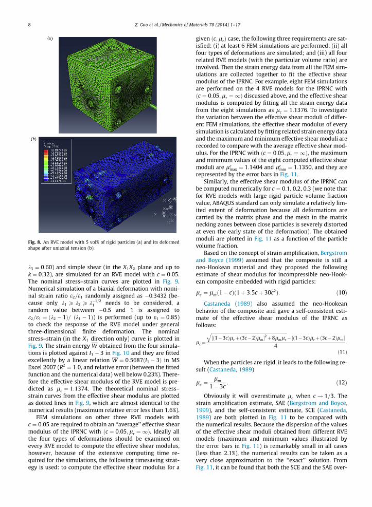
Fig. 8. An RVE model with 5 vol% of rigid particles (a) and its deformedshape after uniaxial tension (b).

8 Z. Guo et al. / Mechanics of Materials 70 (2014) 1–17

k3 ¼ 0:60) and simple shear (in the X1X2 plane and up tok ¼ 0:32), are simulated for an RVE model with c ¼ 0:05.The nominal stress–strain curves are plotted in Fig. 9.Numerical simulation of a biaxial deformation with nomi-nal strain ratio e2=e1 randomly assigned as �0.3432 (be-cause only k1 P k2 P k�1=2

1 needs to be considered, arandom value between �0:5 and 1 is assigned toe2=e1 ¼ ðk2 � 1Þ= ðk1 � 1Þ) is performed (up to e1 ¼ 0:85)to check the response of the RVE model under generalthree-dimensional finite deformation. The nominalstress–strain (in the X1 direction only) curve is plotted inFig. 9. The strain energy W obtained from the four simula-tions is plotted against I1 � 3 in Fig. 10 and they are fittedexcellently by a linear relation W ¼ 0:5687ðI1 � 3Þ in MSExcel 2007 (R2 ¼ 1:0, and relative error (between the fittedfunction and the numerical data) well below 0.23%). There-fore the effective shear modulus of the RVE model is pre-dicted as lc ¼ 1:1374. The theoretical nominal stress–strain curves from the effective shear modulus are plottedas dotted lines in Fig. 9, which are almost identical to thenumerical results (maximum relative error less than 1.6%).

FEM simulations on other three RVE models withc ¼ 0:05 are required to obtain an ‘‘average’’ effective shearmodulus of the IPRNC with ðc ¼ 0:05;lr ¼ 1Þ. Ideally allthe four types of deformations should be examined onevery RVE model to compute the effective shear modulus,however, because of the extensive computing time re-quired for the simulations, the following timesaving strat-egy is used: to compute the effective shear modulus for a

given ðc;lrÞ case, the following three requirements are sat-isfied: (i) at least 6 FEM simulations are performed; (ii) allfour types of deformations are simulated; and (iii) all fourrelated RVE models (with the particular volume ratio) areinvolved. Then the strain energy data from all the FEM sim-ulations are collected together to fit the effective shearmodulus of the IPRNC. For example, eight FEM simulationsare performed on the 4 RVE models for the IPRNC withðc ¼ 0:05;lr ¼ 1Þ discussed above, and the effective shearmodulus is computed by fitting all the strain energy datafrom the eight simulations as lc ¼ 1:1376. To investigatethe variation between the effective shear moduli of differ-ent FEM simulations, the effective shear modulus of everysimulation is calculated by fitting related strain energy dataand the maximum and minimum effective shear moduli arerecorded to compare with the average effective shear mod-ulus. For the IPRNC with ðc ¼ 0:05;lr ¼ 1Þ, the maximumand minimum values of the eight computed effective shearmoduli are lc

max ¼ 1:1404 and lcmin ¼ 1:1350, and they are

represented by the error bars in Fig. 11.Similarly, the effective shear modulus of the IPRNC can

be computed numerically for c ¼ 0:1, 0.2, 0.3 (we note thatfor RVE models with large rigid particle volume fractionvalue, ABAQUS standard can only simulate a relatively lim-ited extent of deformation because all deformations arecarried by the matrix phase and the mesh in the matrixnecking zones between close particles is severely distortedat even the early state of the deformation). The obtainedmoduli are plotted in Fig. 11 as a function of the particlevolume fraction.

Based on the concept of strain amplification, Bergstromand Boyce (1999) assumed that the composite is still aneo-Hookean material and they proposed the followingestimate of shear modulus for incompressible neo-Hook-ean composite embedded with rigid particles:

lc ¼ lmð1� cÞð1þ 3:5c þ 30c2Þ: ð10Þ

Castaneda (1989) also assumed the neo-Hookeanbehavior of the composite and gave a self-consistent esti-mate of the effective shear modulus of the IPRNC asfollows:

lc ¼

ffiffiffiffiffiffiffiffiffiffiffiffiffiffiffiffiffiffiffiffiffiffiffiffiffiffiffiffiffiffiffiffiffiffiffiffiffiffiffiffiffiffiffiffiffiffiffiffiffiffiffiffiffiffiffiffiffiffiffiffiffiffiffiffiffiffiffiffiffiffiffiffiffiffi½ð1�3cÞlrþð3c�2Þlm�

2þ8lmlr

q�½ð1�3cÞlrþð3c�2Þlm�

4:

ð11Þ

When the particles are rigid, it leads to the following re-sult (Castaneda, 1989)

lc ¼lm

1� 3c: ð12Þ

Obviously it will overestimate lc when c ! 1=3. Thestrain amplification estimate, SAE (Bergstrom and Boyce,1999), and the self-consistent estimate, SCE (Castaneda,1989) are both plotted in Fig. 11 to be compared withthe numerical results. Because the dispersion of the valuesof the effective shear moduli obtained from different RVEmodels (maximum and minimum values illustrated bythe error bars in Fig. 11) is remarkably small in all cases(less than 2.1%), the numerical results can be taken as avery close approximation to the ‘‘exact’’ solution. FromFig. 11, it can be found that both the SCE and the SAE over-

0

0.5

1

1.5

2

0 0.2 0.4 0.6 0.8 1 1.2

Nom

inal

stre

ss

Nominal strain(a) Nominal stress 11P vs. nominal strain 1ε for uniaxial tension simulation

- 10

-8

-6

-4

-2

00 0.1 0.2 0.3 0.4 0.5 0.6 0.7

Nom

inal

stre

ss

Nominal strain

(b) Nominal stress 33P vs. nominal strain 3ε for uniaxial compression simulation

Nom

inal

stre

ss

Nominal strain(c) Nominal shear stress 12P vs. nominal shear strain 12F for simple shear simulation

Nom

inal

tres

s

Nominal Strain(d) Nominal stress 11P vs. nominal strain 1ε for simulation of a biaxial deformation

Fig. 9. Simulation results of an RVE model with 5 vol% of rigid particles: (a) nominal stress P11 vs. nominal strain e1 for uniaxial tension simulation along theX1 axial direction (up to k1 ¼ 1:85); (b) nominal stress P33 vs. nominal strain e3 for uniaxial compression simulation along the X3 axial direction (up tok3 ¼ 0:6); (c) nominal shear stress P12 vs. nominal shear strain F12 for simple shear simulation in the X1X2 plane (up to k ¼ F12 ¼ 0:32); (d) nominal stressP11 vs. nominal strain e1 for simulation of a biaxial deformation with nominal strain ratio e1=e2 ¼ �0:3424. The theoretical nominal stress–strain curve fromthe effective shear modulus is plotted as a dotted line in each figure.

W

I1-3

Fig. 10. Average strain energy W vs. I1 � 3 for four numerical simulationsof an RVE model with 5 vol% of rigid particles. The linear fitting curve isplotted as a solid line.

0

2

4

6

8

10

0 0.1 0.2 0.3

Effe

ctiv

e sh

ear

mod

ulus

Particle volume fraction c

Rigid Particles

TPM

SAE

SCE

Numerical

Fig. 11. The effective shear moduli computed from numerical homoge-nization for IPRNC with rigid particles are compared with the SAE, SCE,and TPM predictions.

Z. Guo et al. / Mechanics of Materials 70 (2014) 1–17 9

estimate lc when c > 0:1. When c ¼ 0:05, the prediction ofthe SCE and the SAE are about 3.42% and 4.39% larger thanthe numerical result, respectively. The errors increase up to8.47% and 12.8% when c ¼ 0:1. For moderate particle vol-ume fraction c ¼ 0:2, 44.3% and 33.9% errors are intro-

duced to the SCE and the SAE predictions, respectively.The SCE result is actually not useable when c > 0:2: it willoverestimate three times the value of lc when c ¼ 0:3. TheSAE prediction overestimate lc by 39.8% when c ¼ 0:3.

10 Z. Guo et al. / Mechanics of Materials 70 (2014) 1–17

Because the large deformation estimates for PRC cannotwell predict the effective modulus of the IPRNC with rigidparticles, the classical results for PRC in infinitesimal defor-mation regime are examined. Since the formula proposedby Christensen and Lo (1979) based on the three phasemodel (TPM) for the effective shear modulus of the linearelastic PRC agrees very well with the numerical homogeni-zation results under small strain (Segurado and Llorca,2002) and is relatively simple, it is chosen to be comparedwith our numerical results under large deformation(Fig. 11). Surprisingly, the TPM model originally developedfor linear elastic PRC provides a much better predictionthan the large deformation formulae. The differences be-tween the predictions of the TPM model and the numericalresults are only 0.39%, 2.05%, 0.22%, 5.08% for c ¼ 0:05, 0.1,0.2, and 0.3, respectively.

Recently Avazmohammadi and Castaneda (2012) pro-posed a TSO model to estimate the strain energy functionof the IPRNC with rigid inclusions. In this model the behav-ior of the composite is no longer assumed as neo-Hookeantype. Although the explicit formula of the strain energyfunction for general deformation status is rather lengthy(which reflect the complex nature of the problem), theexpression can be significantly simplified for special cases

Fig. 12. The nominal stress–deformation curves predicted by TSO model for (tension), and (c) simple shear simulations respectively. The numerical results a

such as uniaxial tension, simple shear, equi-biaxial tension(which is equivalent to uniaxial compression). The stressresults from the numerical simulations of the uniaxial ten-sion (UT), simple plane shear (PS), and uniaxial compres-sion (UC, which is equivalent to the equi-biaxial tension,ET) loading cases are plotted in Fig. 12 and compared withthe TSO model. When the volume fraction of the particles cis small (i.e., c ¼ 5%, 10%), the curves predicted by the TSOmodel fit the numerical results very well for all cases (rel-ative error less than 3.7%). This implies that the mechanicalresponses of the composites predicted by the TSO modelare very close to the neo-Hookean model within the re-gime that the numerical simulation can reach. This is fur-ther verified by the almost linear W vs. I1 � 3 curves ofthe TSO model in Fig. 13 for three loading cases. Whenthe volume fraction of the particles increases (i.e.,c ¼ 20%, 30%), though the stress and strain energy pre-dicted by the TSO model is slightly smaller than thenumerical results (relative errors up to 14%, Figs. 12 and13c,d), the relations between W vs. I1 � 3 are still veryclose to linear within the moderate deformation regime.We note that the TSO model will behave differently fromneo-Hookean model when the deformation of the IPRNCis significantly large.

a) uniaxial tension, (b) uniaxial compression (equivalent to equi-biaxialre plotted for comparison.

Fig. 13. The strain energy W vs. I1 � 3 curves predicted by TSO model for IPRNC with rigid particles. The volume fraction of the particles c = (a) 5%, (b) 10%,(c) 20%, and (d) 30%, respectively. The numerical results are plotted for comparison.

Z. Guo et al. / Mechanics of Materials 70 (2014) 1–17 11

4.4. Particles 100 times stiffer than matrix

FEM simulations are carried out on the IPRNC with largebut finite stiffness contrast between particles and matrix(lr ¼ 100). Again the effective shear modulus are obtainedby simulations of four types of deformations, i.e., uniaxialtension along the X1 axial direction (up to k1 ¼ 1:46), uniax-ial compression along the X3 axial direction (up tok3 ¼ 0:59), simple shear in the X1X2 plane (up tok ¼ 0:77), and general biaxial deformation (e2=e1 ¼ 0:8116up to e1 ¼ 0:24) on an RVE with c ¼ 0:1. The nominalstress–strain curves are shown in Fig. 14(a)–(c) for uniaxialtension, uniaxial compression and simple shear simula-tions, while the strain energy W computed in the four sim-ulations of this RVE is plotted against I1 � 3 in Fig. 14(d).The observed linear relation between W and I1 � 3 is fittedby �W ¼ 0:6457ðI1 � 3Þ (R2 ¼ 1 in MS Excel 2007). The effec-tive shear moduli computed from numerical homogeniza-tion for the IPRNC with lr ¼ 100 are compared with theSCE, TPM predictions in Fig. 15. The variations representedby the error bars are all below 4.25% (Fig. 15). The TPMmodel matches the numerical results very well and the dif-ferences for c ¼ 0:05, 0.1, 0.2, 0.3 are only 0.41%, 0.96%,0.22% and 3.82%, respectively. The SCE result will overesti-

mate the shear modulus significantly when c > 0:1, and therelative errors are 3.14%, 8.69%, 36.39% and 123.77% forc ¼ 0:05, 0.1, 0.2, 0.3, respectively.

4.5. Particles 10 times stiffer than matrix

To explore the case that the particle stiffness is compa-rable to the matrix stiffness, a set of simulations is per-formed for lr ¼ 10 in ABAQUS. Because previously theuniaxial tension and the uniaxial compression deforma-tions have already been investigated extensively to verifythe isotropy of the RVE models, only simple shear and gen-eral biaxial simulations are required. To validate the neo-Hookean model for the IPRNC, eight series of biaxial simu-lations (e2=e1 ¼ 1, 0.8, 0.6, 0.4, 0.2, 0, -0.2, -0.4) as well asthe simple shear simulation (up to k ¼ 1:0) are performedon an RVE model with c ¼ 0:2 to cover a significant amountof general deformations. All the W vs. I1 � 3 data from 34FE simulations (9 biaxial, 3 simple shear, 12 uniaxial ten-sion and 10 uniaxial compression simulations) for theIPRNC with ðc ¼ 0:2;lr ¼ 10Þ is fitted by the linear relation�W ¼ 0:7480ðI1 � 3Þ (e.g., l ¼ 1:4960) in Fig. 16, which is

consistent with the effective shear modulus obtained fromthe uniaxial tension simulations in Section 4.2

Nom

inal

str

ess

Nominal strain(a) Nominal stress vs. nominal strain for uniaxial

tension simulation

Nom

inal

str

ess

Nominal strain

(b) Nominal stress vs. nominal strain for uniaxialcompression simulation

Nom

inal

str

ess

Nominal strain

(c) Nominal shear stress vs. nominal shear strain for simpleshear simulation

I1-3

(d) Strain energy W vs. 1 3I −

Fig. 14. The nominal stress–strain curves are shown in (a), (b) and (c) for uniaxial tension, uniaxial compression and simple shear simulations respectively,while the obtained strain energy W is plotted against I1 � 3 for an RVE (c ¼ 0:1; lr ¼ 100) in (d).

0

1

2

3

4

5

6

0 0.1 0.2 0.3

Eff

ecti

ve s

hear

mod

ulus

Particle volume fraction c

µr = 100

TPM

SCE

Numerical

Fig. 15. The effective shear moduli computed from numerical homoge-nization for IPRNC with lr ¼ 100 are compared with the SCE, TPMpredictions.

W

I1-3

Fig. 16. All the W vs. I1 � 3 data from 34 FE simulations (9 biaxial, 3simple shear, 12 uniaxial tension and 10 uniaxial compression simula-tions) for the IPRNC ðc ¼ 0:2;lr ¼ 10Þ are fitted by the linear relation�W ¼ 0:7480ðI1 � 3Þ (R2 ¼ 0:9998).

12 Z. Guo et al. / Mechanics of Materials 70 (2014) 1–17

(l ¼ 1:4958). The maximum and minimum effective shearmoduli from individual simulation are lc

max ¼ 1:5190 andlc

min ¼ 1:4526, which implies the variations of the effective

shear moduli are within 4.5%. This clearly indicates thatthe IPRNC can be well predicted by a neo-Hookean model.

The numerical results for the effective shear modulusare plotted in Fig. 17 together with the predictions of theSCE and TPM models, and the reported dispersions in the

Eff

ecti

ve s

hear

mod

ulus

Particle volume fraction c

µr = 10

Fig. 17. The effective shear moduli computed from numerical homoge-nization for IPRNC with lr ¼ 10 are compared with the SCE and TPMpredictions.

Eff

ecti

ve s

hear

mod

ulus

Particle volume fraction c

µr = 0.5

Fig. 19. The effective shear moduli computed from numerical homoge-nization for IPRNC with lr ¼ 0:5 are compared with the SCE and TPMpredictions.

Z. Guo et al. / Mechanics of Materials 70 (2014) 1–17 13

numerical simulation are less than 4.56%. Again the TPMmodel represents an excellent approximation of thenumerical results and the maximum difference forc ¼ 0:3 is only 1.8%. The SCE model still overestimates

Nom

inal

stre

ss

Nominal strain(a) Nominal stress vs. nominal strain for uniaxial

tension simulation

Nom

inal

stre

ss

Nominal strain(c) Nominal shear stress vs. nominal shear strain for

simple shear simulation

Fig. 18. The nominal stress–strain curves are shown in (a), (b) and (c) for uniaxiawhile the obtained strain energy W is plotted against I1 � 3 for an RVE (c ¼ 0:3

the shear modulus by 1.65%, 4.41%, 12.36% and 21.32%,respectively, for c ¼ 0:05, 0.1, 0.2, 0.3, though the intro-duced error for a given volume fraction is smaller than thatof the IPRNC with lr ¼ 100. This is expected because the

Nom

inal

stre

ss

Nominal strain(b) Nominal stress vs. nominal strain for uniaxial

compression simulation

W

I1-3(d) Strain energy W vs. 1 3I −

l tension, uniaxial compression and simple shear simulations respectively,; lr ¼ 0:5) in (d).

14 Z. Guo et al. / Mechanics of Materials 70 (2014) 1–17

difference between the stiffness of the particles and thematrix is smaller due to the reinforcement of less stiffparticles.

Fig. 20. Undeformed (a) and deformed (b) simple ‘‘one particle in thecentre’’ unit cell model. The shown deformation is 100% uniaxial tension.

4.6. Matrix twice stiffer than particles

In previous simulations, the particles are always stifferthan the matrix. The opposite case (i.e., the matrix is stifferthan the particles) is considered here to fully examine theeffect of stiffness contrast between particles and matrix. Asmall stiffness contrast (lm=lr ¼ 2, or lr ¼ 0:5) is used tomake relatively large deformation possible in the numeri-cal simulation (the convergence problem usually occursat relatively moderate deformation in previous simula-tions, which partially comes from the large stiffness con-trast, i.e., lr=lm P 10). The FEM simulations of uniaxialtension (up to k1 ¼ 2:0), uniaxial compression (up tok3 ¼ 0:17), simple shear (up to k ¼ 2:40), and general biax-ial (e2=e1 ¼ �0:4025 up to e1 ¼ 1:0) deformation are per-formed on an RVE with c ¼ 0:3. The strain energy data �Wfrom all the 4 simulations are fitted in Fig. 18(d) and theobtained effective shear modulus lc ¼ 0:8296. The nomi-nal stress–strain curves are shown in Fig. 18(a)–(c), whichare almost identical to the theoretical results based on thecomputed effective shear modulus. This suggests that theIPRNC’s response at significant stretch still follows theneo-Hookean model’s prediction.

The effective shear moduli derived from the FEM simu-lation results are shown in Fig. 19 with maximum disper-sions represented by error bars (all less than 0.7%). Thenumerical results are also compared with the theoreticalapproximations of the SCE and TPM models. Because thestiffness contrast between the particles and the matrix issmall, the effective shear moduli of the IPRNC are closeto the shear modulus of the matrix. It is then not surprisingthat both the SCE and TPM models agree well with the

Table 1Deformation range represented by I1 for all the FE simulations.

c lr/lm

0.5 10 100 1

0.05 17.55 (k = 4.13) 4.96 (k = 1.98) 3.87 (k = 1.62) 4.5 (k = 1.84)13.71 (k = 0.14) 6.31 (k = 0.32) 3.74 (k = 0.58) 5.19 (k = 0.39)13.68 (k = 3.26) 4 (k = 1) * 4 (k = 1) * 3.21 (k = 0.45)5.03 5.66 3.41 4.53

0.1 17.16 (k = 4.08) 4.4 (k = 1.81) 3.58 (k = 1.49) 3.31 (k = 1.35)17.79 (k = 0.11) 5.02 (k = 0.41) 3.77 (k = 0.58) 3.66 (k = 0.60)10.42 (k = 2.72) 4 (k = 1) * 3.60 (k = 0.77) 3.08 (k = 0.28)8.17 4.49 3.47 3.3

0.2 14.36 (k = 3.71) 4.22 (k = 1.75) 3.35 (k = 1.37) 3.05 (k = 1.13)19.63 (k = 0.10) 4.29 (k = 0.49) 3.41 (k = 0.67) 3.17 (k = 0.78)11.96 (k = 2.99) 4 (k = 1) * 3.6 (k = 0.77) 3.06 (k = 0.24)7.81 3.9 3.43 3.25

0.3 13.77 (k = 3.63) 3.51 (k = 1.46) 3.08 (k = 1.17) 3.06 (k = 1.14)11.74 (k = 0.17) 3.92 (k = 0.55) 3.14 (k = 0.8) 3.003 (k = 0.96)8.80 (k = 2.40) 3.53 (k = 0.72) 3.07 (k = 0.27) 3.03 (k = 0.17)5.06 3.43 3.15 3.006

* The simulations finished without convergence problems.

Z. Guo et al. / Mechanics of Materials 70 (2014) 1–17 15

numerical results. The maximum errors for c ¼ 0:3 are only0.36% and 0.76% for the SCE and TPM models, respectively.

4.7. Deformation ranges of the FE simulations

A total number of 152 FE simulations have been per-formed on the 16 RVE models. The strain energy �W com-puted from each FE simulation shows a clear linearproportional relation with I1 � 3, which suggests a neo-Hookean type response and the corresponding effectiveshear modulus can be obtained by data fitting for eachFEM simulation. The dispersions of fitted effective shearmoduli are within 7.5% as shown in Figs. 10, 12, 14 and 16.

It should be noted that convergence is a big issue in ournumerical simulations even for RVE models with very re-fined mesh (e.g., with more than 200,000 elements), partic-ularly when the stiffness contrast between the particlesand the matrix is large (e.g., lr ¼ 1, 100). Because wecan only claim the neo-Hookean type response of theIPRNC with the deformations simulated by our FEM simu-lations, it is worthy to report the deformation ranges of theFEM simulations for various IPRNC in Table 1, in which thedeformation range is represented by the maximum I1

reached by the FEM simulations, as well as the principal

W

I1-3

(a) Strain energy W vs. 1 3I − for uniaxial tension simulation

W

I1-3

(c) Strain energy W vs. 1 3I − for s

Fig. 21. The average strain energy W vs. I1 � 3 curves of the simple ‘‘one particleuniaxial compression (b), and simple shear (c).

stretches for uniaxial tension/compression, or nominalshear strain for simple shear deformation. For IPRNCs withparticular volume fraction of particles, the larger the stiff-ness contrast between the particles and the matrix, thesmaller deformation range the FE simulations can reach.For IPRNCs with particular lr=lm, the larger the volumefraction of particles, the more limited the FEM simulations.The reason is that larger volume fraction of particles usu-ally means more severe mesh distortion at the neckingarea between particles due to the deformation localization.It should be noted that the uniaxial tension, pure shear andequibiaxial tension behaviors of an INRNC with(c ¼ 0:1; lr ¼ 1) predicted by Avazmohammadi and Cas-taneda (2012) (as in Fig. 11 there) are very close to neo-Hookean behavior for I1 < 5.

4.8. One particle unit cell model

The simple ‘‘one particle in the centre’’ unit cell model(Fig. 20) is sometimes used in the literature to simulatePRC (Bergstrom and Boyce, 1999). This type of unit cellrepresents composites embedded with cubic arrays ofspheres (Cohen, 2004), which is macroscopically orthotro-pic. To examine the mechanical responses of the IPRNC

W

I1-3

(b) Strain energy W vs. 1 3I − for uniaxial compression simulation

imple shear simulation

in the centre’’ unit cell model for three loading cases: uniaxial tension (a),

16 Z. Guo et al. / Mechanics of Materials 70 (2014) 1–17

with this particular type of microstructure under finitedeformation, FEM simulations of the unit cell model areperformed in ABAQUS for uniaxial tension/compressionand simple shear. The particle volume fraction c ¼ 0:2and there are around 20,000 tetrahedral elements and30,000 nodes in the FEM model. Both the matrix and theparticles are modeled as incompressible neo-Hookeanmaterials with lm ¼ 1 and lr ¼ 10, respectively. In all sim-ulations, PBC is applied to get a good estimate of the realresponse of the composite and a deformed unit cell isshown in Fig. 20(b). The average strain energy W vs.I1 � 3 curves are plotted for three loading cases (Fig. 21).For each loading case, a clear proportional relation be-tween W and I1 � 3 can be observed and the effective shearmoduli predicted from uniaxial tension/compression andsimple shear simulations are lc ¼ 1:6698 (R2 ¼ 0:9999,uniaxial tension), 1:8596 (R2 ¼ 0:9989, uniaxial compres-sion) and 1:4150 (R2 ¼ 1:0, simple shear), respectively.The relative difference is about 27.2%, while for the mul-ti-particle RVE models with ðc ¼ 0:2;lr ¼ 10Þ used in thepaper, the maximum relative difference between effectiveshear moduli predicted by different loading cases is wellbelow 1.2%. The effective modulus predicted by the mul-ti-particle RVE models (c ¼ 0:2, lr ¼ 10) is lc ¼ 1:4946.The comparisons between the results from one-particleunit cell model and multi-particle RVE models suggestthat, although the effective modulus predicted by theone-particle unit cell model is close to the one predictedby multi-particle RVE models (relative error about 20%),the behavior of the one-particle unit cell model is aniso-tropic under finite deformation, as determined by itsorthotropic microstructure. Furthermore, a one-particleunit cell model cannot capture the characteristics of thestress/strain field in the matrix necking zone, which is crit-ical to the strength investigation of the IPRNC. Hence mul-ti-particle RVE models should be used to obtain realisticresponse of IPRNC under finite deformation.

5. Concluding remarks

Three-dimensional RVE models are employed to inves-tigate the mechanical behavior of the IPRNC, in which boththe matrix and the particle reinforcement are incompress-ible neo-Hookean materials. To consider different particlevolume fractions (i.e., c ¼ 0:05, 0.1, 0.2, 0.3), 16 RVE sam-ples (4 for each volume fraction value) with periodicmicrostructures are created. In each RVE, 27 non-overlap-ping identical spheres are randomly distributed in a cubicunit. The isotropy of the random distributions of particlesin the 16 RVE models is then examined, and the RVE mod-els are meshed for finite element computation. Periodicmeshes are generated so that the periodic boundary condi-tions can be applied during the FEM simulations. The meshconvergence study shows that a standard mesh with about80,000 elements can obtain accurate result.

To double check the isotropy of the RVE models’mechanical responses, uniaxial tensions and compressionsalong different directions are simulated for the RVE modelsand the isotropy of the RVE models is verified directly. Thesimulation results of the uniaxial tension and compression

are consistent, which implies that the small-size RVE mod-els used here are sufficient to obtain accurate responses ofthe IPRNC. The computed strain energy data suggests thatthe mechanical response of the IPRNC can be well pre-dicted by an incompressible neo-Hookean model. Materialinstability is not considered in this paper.

Four different particle/matrix stiffness ratios are stud-ied in the FEM simulations: lr=lm ¼ 1 (i.e., rigid parti-cles), 100, 10, 0.5, to investigate the effect of stiffnesscontrast between the particle and the matrix. The follow-ing four types of finite deformations are simulated: uniax-ial tension and compression along coordinate axialdirections and random directions, simple shear, and gen-eral biaxial deformation. All the simulation results (i.e.,RVE with any particle volume fraction, any particle/matrixstiffness ratio and any loading case) show that the averagestrain energy �W is proportional to I1 � 3, which suggeststhat the overall behavior of the IPRNC can be modeled byan incompressible neo-Hookean model. The effective shearmoduli lc of the IPRNCs are obtained by fitting the strainenergy data from the numerical simulation results. Be-cause the dispersion in the values of the obtained moduliis remarkably small in all cases, the numerical results canbe considered as a very close approximation to the ‘‘exact’’effective shear moduli of the IPRNC. They are comparedwith three theoretical models: the self-consistent estimate,SCE (Castaneda, 1989), the strain amplification estimatefor composites with rigid particles, SAE (Bergstrom andBoyce, 1999), and the classical linear elastic three phasemodel, TPM (Christensen and Lo, 1979). It is found thatthe TPM provides very accurate approximation to thenumerical results (maximum relative difference less than5.1%) though it is developed for linear elastic PRC. Eventhough the SCE and the SAE are proposed for neo-Hookeancomposites, they overestimate the effective shear modulusof the IPRNC when the particle volume fraction c > 0:1. Inpresent work, we neglect the viscous behavior of particlereinforced elastomer, which was observed in many exper-iments. Previous works on viscoelasticity (Tang et al.,2008a,b) can be extended in the strategy presented hereto account for the memory of the material.

The numerical approach employed here can be used tostudy the mechanical responses of other composites (e.g.,particle-reinforced composite with matrix of Ogden mod-el) in finite deformation regime. But due to the strongmaterial and geometrical nonlinearity, it is usually muchmore difficult if not impossible to construct a simple con-stitutive model to fit the obtained numerical results.

In the numerical simulations, it is usually assumed thatthe particle fillers will not change the mechanical proper-ties of the matrix. However, many researchers argued that,for elastomers, the fillers may alter the effective crosslink-ing density in the elastomeric phase and therefore affectthe mechanical properties of the matrix (a detailed discus-sion can be found in Bergstrom and Boyce (1999)). Becauseof this, the numerical results are not compared with the fi-nite deformation experimental data rarely available in theliterature.

We note that mesh of the matrix necking zone betweenclose particles is very challenging and severe deformationlocalization may happen when the stiffness contrast be-

Z. Guo et al. / Mechanics of Materials 70 (2014) 1–17 17

tween the particle and the matrix is large. Hence conver-gence is a big issue in our numerical simulation even forRVE models with very refined mesh (e.g., with more than200,000 elements). For example, it is only possible to reachmoderate deformation state for some cases (e.g., I1 ¼ 3:06,or 14% tension for the IPRNC with ðlr ¼ 1; c ¼ 0:3Þ). Formuch less critical case like the IPRNC with ðlr ¼ 0:5;c ¼ 0:3Þ, huge deformation can be reached (i.e., 313% ten-sion or 86% compression). The numerical results showclearly that up to the deformations the FEM simulationscan reach (that is, until there is a convergence problem),all the numerical results of �W and I1 � 3 can be fitted al-most exactly using the linear relation suggested by theincompressible neo-Hookean model. Therefore it is safeto conclude that the mechanical behavior of the IPRNCstudied here can be well modeled by another incompress-ible neo-Hookean model within the limit of current FEMsoftware ABAQUS.

Acknowledgement

The financial support from NSFC (No. 11272362,11272364, China), Ministry of Education (No. 313059, Chi-na), the Fundamental Research Funds for the Central Uni-versities (CDJZR112248801, CDJZR12110072, China), StateKey Laboratory of Coal Mine Disaster Dynamics and Con-trol (Chongqing University, China), Opening fund of StateKey Laboratory of Nonlinear Mechanics (China), and EPSRC(EP/H016619, UK) is greatly appreciated.

References

ABAQUS, 2010. Analysis User’s Manual, Version 6.10. SIMULIA Inc.Avazmohammadi, R., Castaneda, P.P., 2012. Tangent second-order

estimates for the large-strain, macroscopic response of particle-reinforced elastomers. J. Elast., 1–45.

Bergstrom, J.S., Boyce, M.C., 1999. Mechanical behavior of particle filledelastomers. Rubber Chem. Technol 72, 633–656.

Castaneda, P.P., 1989. The overall constitutive behavior of nonlinearlyelastic composites. Proc. Roy. Soc. A: Math. Phys. Engng. Sci. 422,147–171.

Chen, C., Lu, T.J., Fleck, N.A., 1999. Effect of imperfections on the yieldingof two-dimensional foams. J. Mech. Phys. Solids 47, 2235–2272.

Christensen, R.M., Lo, K.H., 1979. Solutions for effective shear propertiesin three phase sphere and cylinder models. J. Mech. Phys. Solids 27,315–330.

Cohen, I., 2004. Simple algebraic approximations for the effective elasticmoduli of cubic arrays of spheres. J. Mech. Phys. Solids 52, 2167–2183.

deBotton, G., Hariton, I., Socolsky, E.A., 2006. Neo-Hookean fiber-reinforced composites in finite elasticity. J. Mech. Phys. Solids 54,533–559.

Drugan, W.J., Willis, J.R., 1996. A micromechanics-based nonlocalconstitutive equation and estimates of representative volumeelement size for elastic composites. J. Mech. Phys. Solids 44, 497–524.

Guo, Z.Y., Caner, F., Peng, X.Q., Moran, B., 2008. On constitutive modellingof porous neo-Hookean composites. J. Mech. Phys. Solids 56, 2338–2357.

Guo, Z.Y., Peng, X.Q., Moran, B., 2006. A composites-based hyperelasticconstitutive model for soft tissue with application to the humanannulus fibrosus. J. Mech. Phys. Solids 54, 1952–1971.

Guo, Z.Y., Peng, X.Q., Moran, B., 2007. Large deformation response of ahyperelastic fibre reinforced composite: theoretical model andnumerical validation. Compos. A: Appl. Sci. Manufact. 38, 1842–1851.

Guth, E., 1945. Theory of filler reinforcement. J. Appl. Phys. 16, 20–25.Hashin, Z., 1985. Large isotropic elastic-deformation of composites and

porous-media. Int. J. Solids Struct. 21, 711–720.Hashin, Z., Shtrikman, S., 1963. A variational approach to the theory of the

elastic behaviour of multiphase materials. J. Mech. Phys. Solids 11,127–140.

Hill, R., 1965. A self-consistent mechanics of composite materials. J. Mech.Phys. Solids 13, 213–222.

Hill, R., 1972. Constitutive macro-variables for heterogeneous solids atfinite strain. Proc. Roy. Soc. Lond. A: Math. Phys. Sci. 326, 131–147.

Hohe, J., Becker, W., 2003. Effective mechanical behavior of hyperelastichoneycombs and two-dimensional model foams at finite strain. Int. J.Mech. Sci. 45, 891–913.

Imam, A., Johnson, G.C., Ferrari, M., 1995. Determination of the overallmoduli in second-order incompressible elasticity. J. Mech. Phys.Solids 43, 1087–1104.

Kerner, E.H., 1956. The elastic and thermo-elastic properties of compositemedia. Proc. Phys. Soc. Lond. B 69, 808.

Khisaeva, Z.F., Ostoja-Starzewski, M., 2006. On the size of RVE in finiteelasticity of random composites. J. Elast. 85, 153–173.

Kouznetesova, V., 2002. Computational Homogenization for the Multi-scale Analysis of Multi-phase Materials. Eindhoven University ofTechnology.

Lopez-Pamies, O., 2010. An exact result for the macroscopic response ofparticle-reinforced neo-Hookean solids. J. Appl. Mech. 77, 021016.

Michel, J.C., Moulinec, H., Suquet, P., 1999. Effective properties ofcomposite materials with periodic microstructure: a computationalapproach. Comput. Method Appl. Mech. Engrg. 172, 109–143.

Miehe, C., Schroder, J., Becker, M., 2002. Computational homogenizationanalysis in finite elasticity: material and structural instabilities on themicro- and macro-scales of periodic composites and their interaction.Comput. Method Appl. Mech. Engrg. 191, 4971–5005.

Moraleda, J., Segurado, J., Llorca, J., 2007. Finite deformation of porouselastomers: a computational micromechanics approach. Phil. Mag. 87,5607–5627.

Moraleda, J., Segurado, J., Llorca, J., 2009. Finite deformation ofincompressible fiber-reinforced elastomers: a computationalmicromechanics approach. J. Mech. Phys. Solids 57, 1596–1613.

Ogden, R.W., 1974. Overall moduli of nonlinear elastic composite-materials. J. Mech. Phys. Solids 22, 541–553.

Segurado, J., Llorca, J., 2002. A numerical approximation to the elasticproperties of sphere-reinforced composites. J. Mech. Phys. Solids 50,2107–2121.

Segurado, J., Llorca, J., 2005. A computational micromechanics study ofthe effect of interface decohesion on the mechanical behavior ofcomposites. Acta Mater. 53, 4931–4942.

Segurado, J., Llorca, J., 2006. Computational micromechanics ofcomposites: the effect of particle spatial distribution. Mech. Mater.38, 873–883.

Tang, S., Greene, M.S., Liu, W.K., 2012a. A renormalization approach tomodel interaction in microstructured solids: application to porouselastomer. Comput. Method Appl. Meth. 217, 213–225.

Tang, S., Greene, M.S., Liu, W.K., 2012b. Two-scale mechanism-basedtheory of nonlinear viscoelasticity. J. Mech. Phys. Solids 60, 199–226.

Tang, S., Guo, T.F., Cheng, L., 2008a. Mode mixity and nonlinear viscouseffects on toughness of interfaces. Int. J. Solids Struct. 45, 2493–2511.

Tang, S., Guo, T.F., Cheng, L., 2008b. Rate effects on toughness in elasticnonlinear viscous solids. J. Mech. Phys. Solids 56, 974–992.

Torquato, S., 1998. Effective stiffness tensor of composite media: II.Applications to isotropic dispersions. J. Mech. Phys. Solids 46, 1411–1440.