1

Mechanical measurements at the micron and nanometer scales

Wolfgang G. Knauss*, Ying Huang

Graduate Aeronautical Laboratories, California Institute of Technology

Pasadena, CA 91125, USA

Ioannis Chasiotis

Mechanical and Aerospace Engineering, University of Virginia

Charlottesville, VA 22904, USA

Abstract

Experimentation at the micron level requires specific tools and methods. It will be

illustrated how some of these tools have to be combined to achieve this goal. Because the

determination of strains at the micron-and nano scales has been explored with the aid of probe

microscopy, attention needs to be devoted to the limitations of digital image correlation. In this

context it is illustrated how the results of the correlation method are affected by several process

parameters, such as subset size, out-of-plane deformation, displacement gradients and scanning

noise introduced in measurements.

We also present measurements of material fracture on small, elliptically perforated

(MEMS) specimens under tension via specially constructed equipment. Of particular interest is

how the failure strength of polycrystalline silicon (grain size ~0.3 µm) is influenced by the

magnitude of the notch radius (one to eight microns) and the stress concentration factor (three to

* Tel.: (626) 395-4524; Fax: (626) 449-2677. E-mail address: wgk@caltech.edu (W. G. Knauss)

2

ten). It is demonstrated that when the notch radius falls below three microns, the strength of the

material is no longer governed by the critical stress criterion that controls failure initiation for

larger radii (e.g. eight µm or larger). In fact, the stress gradient plays a significant role in the

failure process, which is explained in terms of the statistical spatial distribution of small flaws or

cracks and the size of the zone at the notch tip under high stress. Failure stresses increase by a

factor of two or more at a characteristic size of one micron.

Keywords: Digital Image Correlation; probe microscopy; MEMS perforated specimens;

elliptical notches; failure strength; size effects

1. Introduction

Engineering has been on a multi-year path of effecting designs at decreasingly smaller scales,

and mechanics has played a significant role in this endeavor for nearly two centuries. Besides

providing principles, theories and other guides based on physics to accomplish continuing

refinements and increased detailing of structural reliability, mechanics is providing significant

input into the behavior of materials. Wherever materials are thus called upon to transmit loads,

the laws of mechanics must be obeyed. This long trend has been accelerated during the last

decade by the development of tiny electronic devices which required manufacturing

subcomponents at still smaller size scales unheard of only two or three decades ago. This ability

to manufacture micro-and nano-sized components of many shapes and for many purposes, as

well as the need to assure their durability, necessarily entail the need to both analyze and

experimentally explore structures at that size scale. An important field of endeavor in that

context is also the mechanics of materials at the nano-scale, whether exemplified through

3

multiple phases of the same or of different materials (nano-composites). In this context

mechanics contributes the tools to quantify physical phenomena for predictive purposes which

govern the mechanical response at that size level. These phenomena typically deal with the

interaction of inhomogeneous material domains under common stress, with interactions of

different solids across interfaces, and at a very fundamental level, with the strength

characteristics of all solids that originate at the atomic and supra-atomic level.

Whether interest centers thus on materials issues or on the design of micro- and nano-devices,

mechanical reliability issues demand the capability for analytical and experimental

investigations. Regarding analytical needs, modern-day computers allow for a large set of highly

flexible algorithms, so that scale issues do not present a hindrance per se. This is not true with

regard to experimental work. Though experimental mechanics has drawn on a large increase in

experimental methods during the last few decades, notably high-resolution optical tools,

observation and measurements at the sub-optical level still pose a serious challenge. The reason

is that there are few media that allow probing at such a small size scale. Moreover, it is not

necessarily sufficient to be able to image phenomena at the nano-scale, but mechanics requires

precision in measuring deformations which entails not only high-resolution capabilities, but also

an ability to reproduce the position of image points with “high precision”. The reason is that the

determination of relative deformations requires two images for comparison purposes to extract

strain measures.

To date, all imaging tools having a sufficient spatial resolution are candidates for dealing with

amorphous micro- and nano-structures. They include, thus, the scanning electron- and the

transmission electron microscopes, as well as the more recent advents of scanning tunneling and

4

atomic force microscopes. While affording imaging capability at the nano-scale, their ability to

reproduce the requisite multi-scan precision is more in doubt.

For ordered material structures, x-ray diffraction methods afford a very powerful means to

evaluate strain fields in very small domains. Though this is not a trivial task compared to

operations involving optical interferometry, the capability as well as past experience exist to be

exploited.

To date, we have explored the application of probe microscopy to the study of mechanics

problems at the micron and sub-micron domain. The inducement of these devices is primarily

given through their high-resolution capability for surface imaging. Of primary interest is then the

pursuit of the question as to what degree the properties at the nano-scale differ from those at the

macroscopic level.

To this end we discuss in the sequel two topics: The first relates to the digital image correlation

method for extracting strain fields from images scanned before and after deformation, and

particularly to the limitations imposed by the method on deformation resolution. The second

topic addresses measurements at the micron-scale to determine the influence of stress gradients

on the fracture initiation in the vicinity of notches in poly-crystalline silicon which are

dimensioned in terms of microns. In this connection, several prerequisites for testing at the

micro-scale are reviewed: The “test machine”; means of gripping small specimens; design and

manufacture of the elliptically perforated specimens and, finally, the measurement results are

discussed.

5

2. Limitations of the Digital Image Correlation Method

Probe microscopy offers the capability of performing surface measurements with nanometer

resolution. In mechanics applications, dual records are needed for determining deformation

field(s), one before the application of load and one afterwards to determine from both of them

the deformation field of points in the observed surface. This process needs to occur with

sufficient precision so that (suitably normalized) differences in the displacement field allow for

extraction of the strain field. Because of the sub-micron resolution requirement, many of the

traditional fine optical methods, limited by the wavelength of light (about one micron) as the

smallest length unit, are no longer effective. Instead, the sub-micron resolution capability of

probe microscopes allows evaluation of two-dimensional deformation fields through the method

of digital image correlation.

Digital image correlation was first applied to solid mechanics problems by Peters, Ranson and

Sutton (1982, 1983) who used the method on laser speckle images. Subsequent publications have

improved the method as recorded in an extensive set of papers with references (Sutton et al,

1983, 1984; Bruck, McNeil and Sutton, 1989) forming a representative set. The method was also

extended to measuring three-dimensional displacement fields through stereo imaging (Luo et al,

1993). In 1990, Vendroux and Knauss (Vendroux, 1990, Vendroux and Knauss, 1998) adapted

this method to identify displacements from topographical images obtained with a scanning

tunneling microscope. While the technique has proven to be effective, though not without

difficulties, an improved quantitative assessment of the precision of the method is needed.

We explore in the sequel the limitations of this method by examining its sensitivity to a set of

6

parameters, namely the subset size, i.e., the size of the number of points employed in the

correlation; the influence of displacement gradients; out-of-plane deformations; high frequency

noise; the role of interpolation; and the proper treatment of inhomogeneous deformations. We

pursue this goal by starting with mathematically well-defined continuous functions (sine waves)

and generate from them “deformed” traces according to a mathematically prescribed

displacement function. These “original” and “deformed” traces become the input to the

correlation process, with the quality of the correlation result being judged in terms of the

closeness of the displacement or strain output of the process to the respective prescriptions.

2.1. One-dimensional Image Correlation

The understanding of these issues is greatly simplified by first addressing the motivating

questions through a one-dimensional treatment, in the wake of which a two-dimensional

treatment is explored more efficiently. Anticipating these later results we note that the one-

dimensional account resolves most, if not all, of the issues of interest.

In one dimensional image correlation one deals with line “images” instead of two-dimensional

surface profiles. In a brief review of the theoretical basis we assume only that the deformations

are sufficiently small to preserve the characteristic features of the profile. The method is first

demonstrated on the simple case of a continuous, sinusoidal signal subject to various in-line

deformation prescriptions. Once the one-dimensional method has been proven useful, several

parameters are considered and their influence on the correlation is examined.

7

2.1.1. Theoretical Background

With reference to Figure 1 let F be a point of coordinate x in an undeformed one-dimensional

configuration and let f(x) be the height of the profile at F.

After deformation, the point F is mapped into )~(xgG = , where

)(~ xuxx += (1)

with u denoting the in-line displacement of F, and

)()()~( xwxfxg += (2)

with w denoting the surface-normal displacement.

Let F0 of coordinate x0 be mapped into G0 of coordinate 0~x and S be a subset around point F0.

Assuming that S is “properly sized”, the deformation (2) can be expanded as

...))((21))(()(~ 2

002

2

000 +−+−++= xxxdx

udxxxdxduxuxx (3)

We deal first with situations requiring terms to first order.

Define a least square (correlation) coefficient C on the subset S as

∫

∫ −=

S

S

dSxf

dSxgxfC

)(

)]~()([2

2

(4)

It is obvious that C is zero when the mapping is exact (the correlation is perfect). Assuming a

8

linear deformation within the subset and considering only out-of-plane translation, the coefficient

at point F0 can be rewritten as

∫

∫ −++−+=

S

S

dxxf

dxxxxdxduxuxgxwxf

xC2

20000

0 )(

)]})(()([)()({)( (5)

Define the three-dimensional vector

)}(),(),({)( xwxdxduxuxP = (6)

so that C=C(x, P) and equation (5) becomes

∫∫ −++−+

=S

S

dxxf

dxxxxPxPxgxPxfPxC

2

20020103

0)(

)]}(*)()([)()({),( (7)

Expanding C(P) as a truncated Taylor series around P0 leads to

))(()()()()()( 00021

000 PPPCPPPPPCPCPC TT −∇∇−+−∇+= (8)

differentiation of which with respect to P on both sides of the equation yields

))(()()( 000 PPPCPCPC −∇∇+∇=∇ (9)

When C reaches a minimum at P, 0)( =∇ PC . Thus (9) becomes

)())(( 000 PCPPPC −∇=−∇∇ (10)

Solving for P iteratively from (10) renders the solution of this minimization process. This

9

optimization scheme is called the Newton-Raphson method, and the double gradient )(PC∇∇ is

known as the Hessian matrix

3,2,1;3,2,1

2

)(==

∂∂∂=∇∇

jiji PPCPC (11)

Because C may have multiple minima, the initial guess for the “solution” needs to be

“sufficiently close” to the final result. Details for such choices and the evaluation of the

effectiveness of the minimization algorithm alone are discussed in the work of Huang (Huang,

2001).

2.1.2. Subset Size

According to the work of Vendroux and Knauss (1998) and Sutton et al. (1983, 1986), the subset

size is always a critical parameter in the correlation. On the one hand, one assumes that the

subset is sufficiently small so that the deformation within the subset can be represented as linear,

implying that smaller subsets should be preferable. On the other hand, the subset has to include

characteristic features of the signal, so that it can be readily correlated with the deformed subset;

this argues for a larger subset. Therefore, there is reason for a trade-off with an optimum subset

for specific signals and deformations.

Computations show that the subset size has to be chosen to locally include characteristic features

of the profile. Specifically, if the signal contains a dominant frequency, the subset size has to

encompass at least half of this local wavelength.

10

2.1.3. Displacement vs. Displacement Gradient

If the least square correlation coefficient C is plotted as a function of u and du/dx, the function

varies strongly with respect to u, but is rather insensitive to du/dx. This implies that correlation

provides a more accurate result for displacements than for its gradients, which agrees with

previous observations (Vendroux, 1990) that strains calculated from u are better than du/dx

extracted directly from the correlation.

2.1.4. Out-of-Plane Deformation

Scans obtained from probe microscopes before and after deformation are not guaranteed to

remain in the same plane (e.g. Poisson effect), so that locally (linear) out-of-plane deformation

can exist. In the vicinity of a crack tip this spatial dependence could be severe. Such occurrences

prompt the question of whether out-of-plane deformation terms need to be included in the

optimization process. Previous studies by Vendroux and Knauss (1998) found that the addition

of w in equation (5) helped with respect to convergence and precision. Intuition might suggest

that if a constant out-of-plane translation exists, the correlation should yield the same result

regardless of whether that displacement is accounted for in the optimization or not, except that

the minimum of C will not be 0, but a constant difference integrated over the subset.

Computations did not confirm this, but showed instead that the a priori exclusion of the out-of-

plane displacement “w” can induce errors so large that the deduction of in-plane displacements

becomes virtually meaningless. This fact may result from the non-linearity of the minimization

process. Further study on this point was, therefore, devoted to examining the need for

11

out-of-plane gradients to be considered through the addition of linear and quadratic terms to the

out-of-plane displacement expansion: One finds then that the out-of-plane deformation

expansion needs to include all terms to the appropriate order so as to match the actual

displacement functions as closely as possible (see also section 2.1.7 later on).

2.1.5. Uncertainty Associated with High Frequency

We explore next the influence of (random) unwanted signals superposed on the surface profile.

Specifically, we are interested in examining whether the error changes significantly. For

reference purposes we need to state the error involved in correlating the deformation of a smooth

(sinusoidal) profile that is well defined in a mathematical sense. Upon stretching (straining) such

a profile that is specified numerically with an error of 10 –5 one finds that the deformation can be

recovered with an error of less than 10 –5 for all subset sizes, excepting a subset of size 2, if the

minimization operation is performed until the error decreases to that value. This situation cannot

be regenerated if a disturbance is added to the deformed profile. To illustrate this point consider

a (one-dimensional) surface profile in the shape of a square wave possessing a fundamental

length of 20 (non-dimensional) units, and represented by a 10-term Fourier series. Let this profile

be strained by 1% (the fundamental length changes from 20 → 20.2). To this undeformed profile

add a sinusoidal signal possessing a wavelength of 2 (1/10 of the “square carrier wave length”)

and a magnitude equal to only 1% of the basic square wave height. Figure 2 shows that for most

subset sizes the error is now on the order of 10 –3, i.e., the error has increased by two orders of

magnitude over the reference example. This indicates that high frequency uncertainty of only

12

small amplitudes can influence the results rather severely. It appears therefore that filtering the

unwanted disturbance signals from any record should improve the situation (see also section

2.1.7).

2.1.6. Interpolation

When applying digital image correlation to discrete data, interpolation is required since discrete

points generally do not necessarily move in units of pixel spacing. For discrete data interpolation

makes sub-pixel displacement resolution possible. Previous studies (Sutton et al, 1983;

Vendroux and Knauss, 1998) showed that cubic spline interpolation renders better results than

linear and quadratic interpolations. Our studies substantiated this and consequently cubic spline

interpolation has been adopted for all this work.

To examine the effects which the parameters, previously studied by means of smooth and

analytical signals, have on interpolated data, correlation on discrete data subject to uniform in-

plane translation and strains were repeated, but for brevity of presentation the result are not

detailed here Suffice it to say that the results agreed very well with those for continuous signals.

This finding suggests that errors introduced by cubic spline interpolations are negligible

compared to those originating from the algorithm itself.

13

2.1.7. Inhomogeneous Deformation within the Subset

For the following example we use a real AFM scan, but filtered for high frequencies†. Digital

image correlation is generally expected to be applied to inhomogeneous deformations such as, in

the extreme case, those near a crack tip. It is, therefore, important to understand how well

inhomogeneous deformations can be extracted by these means. The answer lies in the trade-off

between the linear representation of the displacement function(s) and the size of the subset. If the

linear approximation is retained the subset must be sufficiently small to allow that

approximation. If the subset increases to the scale where second order terms in the expansion are

necessary, the correlation quality will suffer. This observation is illustrated in Figure 3, which

represents a case for which a u-displacement is provided with a second order term (c.f. figure

caption), which, however, is (intentionally) not accounted for in the displacement expansion

(The minimization depends only on the zeroeth and first order terms). One notes that exclusion

of the second order term in the minimization process clearly increases the error significantly for

the larger subsets.

Next we examine whether the addition of a second order displacement gradient improves the

correlation results for large subset sizes. Using now },,{ 2

2

dxud

dxduu as parameters to represent the

displacement field 2001.001.0 xxu += and w=0, leads to the correlation results of

inhomogeneous deformation applied to the profile as shown in Figure 3. Note that, in contrast to

† In this study, a 10th order low-pass digital Butterworth filter with a cut-off frequency of 15% of the sampling

frequency is used to filter out the high frequency component.

14

the previous case, the correlation error is now well within the tolerance of 10-4 regardless of the

subset size. (observe also the difference in the scale on the ordinate for this and the previous

figure). This result is consistent with the study on the out-of-plane deformations in the sense that

correlation provides virtually exact results when a sufficient number of expansion terms is

included in the displacement representation for the correlation.

The question regarding what “sufficient” means must be answered in the context of physical

knowledge concerning the gradients of the displacement field elative to the size of the subset

used. If one expects, for example, second order terms to be important over the size of the subset,

then, certainly, these terms need to be included for the purpose of minimizing the correlation

coefficient. On the other hand, it would be computationally wasteful (costly) to include third

order terms if they are not needed. Thus, in the event that this heuristic approach is not deemed

sufficiently accurate, the decision has to be made, ultimately, by including a reasonable number

of terms and provide an accuracy evaluation for that number and compare it with the situation for

which one more or one less term is included.

2.2. Two-Dimensional Digital Image Correlation

One difficulty in two-dimensional correlation derives from the fact that, even for an initial

exploration, the number of parameters involved becomes too large if one works with analytical

simulation functions. Therefore, discrete data is used and interpolation between adjacent pixels is

15

needed.

For inhomogeneous deformations, the assumption of linear deformation within a subset is still

useful if sufficiently small subsets can be used. The more dominant the non-linear contribution is

in the deformation, the larger the correlation error. However, if enough non-linear displacement

gradient terms are included to represent the prescribed displacement field, correlation derives

acceptable results regardless of the subset size. Because noise is intrinsic in experimental data, a

calibration method to determine how to filter out high frequency noise is proposed as outlined in

the next section.

3. Probe Microscopy and Digital Image Correlation

The study of both one-dimensional and two-dimensional digital image correlation reveals that

error differences between the undeformed and deformed signals have a significant influence on

the correlation results. Noise is intrinsic in experimental measurements. Therefore, it is important

to understand the nature and characteristics of the noise before one can fully evaluate its

influence on the digital image correlation.

To illustrate this point we consider the noise that originates from measurements on silicon (and

other materials) with a commercial atomic force microscope (AFM). First, the temporal noise,

i.e., when the AFM is not scanning, was collected and its frequency content was analyzed to

determine the dominant frequency range for filtering purposes. A low-pass filter was then

applied and the comparison between the filtered and unfiltered signals analyzed. When the AFM

16

is in the scanning mode, this temporal noise is translated into an inconsistency or uncertainty

between repetitive scans. To explore this behavior further, digital image correlation was applied

to the line profiles from consecutive scans and the results were examined.

3.1. Spatial Uncertainty

A close comparison between supposedly identical scan lines taken from two repeat images

demonstrates that repeatability holds only within limits (up to 3nm) which is consistent with the

amplitude of the temporal noise. Thus, Figure 5 shows two repeat scans, the first one

representing the unfiltered data, and the second the same, but filtered, profile. Although the high

frequency noise has clearly been removed between part (a) and (b), the difference range for the

two traces remains essentially the same.

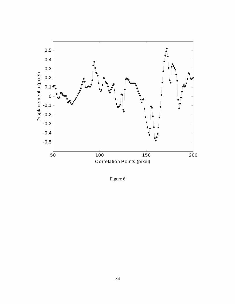
In spite of the fact that the difference between the two traces is relatively small, the uncertainty

between the two line profiles is not negligible when digital image correlation is performed.

Figure 6 represents this evaluation and shows that “artificial” displacements for up to half a pixel

(corresponding to about 5nm) are generated from this inconsistency of repetitive scans. This

“artificial” displacement clouds thus the calculation of real displacements when image

correlation is performed in an experiment.

Because the uncertainty between repetitive scans originates from random temporal noise intrinsic

to the instrument, one can only estimate the size of the error as large as half a pixel, but cannot

eliminate it. It is not possible to “calibrate this error out of the instruments”. Here is a need for

17

improvements in scan precision of probe microscopes that needs to be addressed for further

advances in nano-mechanics.

In this context we note that in two-dimensional scans the AFM can exhibit serious problems,

when the hysteresis of the piezo-ceramic actuator is not compensated. The hysteresis in the in-

plane directions translates successive scans with respect to each other, while the hysteresis in the

out-of-plane direction creates inclination (color band problems) for the scanned image. To make

significant advances in the precision application of AFMs to nanomechanical studies a

mechanism (optical or mechanical) is, therefore, needed to ensure that the probe returns to the

same position after each line scan before moving to the next line (as well as after the whole

image scan). During operation of our commercially available AFM, a closed loop system is used

to monitor the position of the piezoelectric tube and correct for nonlinearities. Due to the random

character of the surface topography of our samples, the hardware closed loop correction system

was considered a more effective solution over alternative software based correction techniques.

These studies have shown so far that DIC can be a powerful tool in the strain field determination

involving very small examination domains. The precision of the method hinges principally on

the precision with which scans can be acquired in a repeat mode over spatially identical domains.

If the error incurred in repeat scans is on the same order as the deformations to be determined the

success will be questionable. Even spatial filtering is not likely to reduce this experimental error

to negligible levels.

18

4. Strength Characterization at the Micron Scale

In this section we review measurements aimed at clarifying to what extent the size scale has an

influence on the failure initiation from stress concentrations at the roots of notches. Although

there are considerable variations in approaches by which the parallel problem is approached in

the macro-domain (centimeter scale), the simplest engineering practice is to associate failure

initiation with the maximum stress at the base of a notch. In the context of device

microfabrication, the same question arises, but there is as yet no experimental assurance that the

initiation stress is (also) independent of the notch geometry, in particular, independent of the

notch radius, even if the local stress concentration is invariant. For this exposition it is useful to

review briefly the equipment requirements, after which we discuss the measurement results and

their implications.

4.1. Description of the Experimental Apparatus

The experimental set-up for subjecting small “dog-bone” shaped specimens to tension is

described in detail in Chasiotis and Knauss (2000), so that a short review suffices here.

Displacements are imposed on the specimen (geometry described below) via an inchworm

actuator slaved by a personal computer and by a dedicated controller. The controller provides for

a measurement of the total system displacement (specimen + loading device) with an accuracy of

4nm for every single step of the actuator. The induced load is measured by a miniature

tension/compression load cell with an accuracy of 10-4N and a maximum capacity of 0.5N. A

miniature y-z translation stage is employed for sample positioning, while the setup allows for

19

rotational adjustments about the x-axis (along the load cell - specimen - inchworm axis) and y-

axis (on the plane of the specimen).

A new gripping method has been developed that makes use of a high viscosity Ultraviolet (UV)

adhesive. This micro-tensile tester is free of accumulated charge effects and facilitates the test of

high strength, or non-linearly behaving materials, making this a universal method for testing thin

films. It represents a significant improvement over the electro-static method advanced by

Tsuchiya et al (1996), which was also used previously in our laboratory. For material strength

characterization that is discussed here, the properties of the adhesive medium relative to the

specimens are not important because only the applied force at failure is needed. When

measurements of the elastics constants were conducted (Chasiotis and Knauss, 2002), the

compliance of the adhesive was measured using the microtensile testing experimental setup and

that value was used in the calculation of the material modulus.

The operation of the newly implemented grip is illustrated in Figure 6. Electrostatic forces are

applied to force the thin polysilicon film to lie flat on the substrate (residual stress gradients may

cause curvature) (Figure 6, I). The glass grip then approaches the flat paddle (Figure 6, II). The

grip is transparent to allow sufficient UV light to pass through for curing the underlying UV

adhesive layer effectively in minimal time. Next, the two surfaces of the substrate and the

specimen paddle which adhere electrostatically and due to any stiction forces, are separated by

reversing the voltage so that the film is repelled by the substrate and adheres to the grip covered

by a thin UV adhesive layer (Figure 6, III). Next, the glue is cured by a short exposure to UV

light. This process eliminates the need of mechanically pressing the grip against the paddle and

the substrate, and thus eliminates the potential flow of the adhesive onto the substrate. It is of

20

interest to note that this gripping provided us with a nearly 100% success rate, which represents

an increase by a factor of two over that achieved with an electrostatic grip.

Specimen alignment was very important in the accurate determination of the failure stress for the

microtensile specimens. The alignment between the specimen and the UV adhesive grip and the

load cell was monitored via a 300x magnification optical microscope.

4.2. Design of Perforated Microtensile Specimens

Specimens with different gage section and internal perforations have been fabricated during

MUMPs35 (Multi User MEMS Processes) run at the Microelectronics Center in North Carolina

(MCNC) (currently Cronos). The main goal was to investigate the existence of size effects in the

measurement of mechanical strength for micron sized geometries. Because of the limitation

imposed by the microfabrication technique, the grain size in samples was constant at about

300nm. Manufacturing processes at MCNC limited the smallest radius of curvature to 1 micron.

The specimens were fabricated with elliptic perforations so that the aspect ratio and notch radii

led to constant stress concentrations under varying notch radii (Table 1). The typical tensile

“bone-shaped” specimen represented a “free-standing beam” (Figure 7) ending in a large paddle

for bond-gripping. The dimensions of the gage section varied from 250x30x2 microns to

700x340x2 microns (Figure 8). More details about the design requirements and the fabrication

processing and post-processing may be found in references by Chasiotis and Knauss (2000) and

Koester et al (2000).

The initial design drew on Neuber’s results (Neuber, 1946) for estimating stress

21

concentration factors during the specimens design phase. For some samples the notch had to be

placed near the specimen edge, because the lateral dimensions of the gage section are limited by

the necessity to include etch holes (Koester et al, 2000). Neuber-type solutions do not strictly

apply in this case and finite element analysis was, therefore, performed to accurately calculate

the stress concentration factors‡ for the final analysis of all geometries under the assumption of

continuum isotropic (in-plane) material properties§. The dimensions of the specimens tested and

the nominal stress concentration factors, K, are shown in table 1.

The stress concentration varied from K=3, for specimens with circular holes, to K=11**, for

specimens with elliptical notches of high aspect ratios. The radius of curvature varied between

ρ=1 and ρ=8 microns. Thus, the radius of curvature of the sharp notch tip varied from 3 up to 25

times the grain size. According to the specifications provided by MCNC (Koester et al, 2000)

microfabrication limitations demanded the minimum feature size to be 2 microns. Therefore,

elliptical and circular holes with radii of curvature as small as 1 µm were incorporated in the

gage section. Typical geometries used in this test sequence are shown in Figure 9.

‡ As a result of the refined (numerical) analysis, the goal of achieving constant stress intensity factors in the

specimens was achieved only approximately.

§ Out of interest these results were also compared with those provided by the approximate solutions of Isida (1955)

and the finite width correction factors calculated by Tan (1988). The agreement of the approximations with the

numerical results was very acceptable.

** The maximum width for the surface micromachined specimens was limited by fabrication considerations

(Chasiotis and Knauss, 2001). The stress concentration for specimens with ρ=8 µm and nominal K=8 was calculated

via our FE model to be K=11 due to the finite width of the perforated specimens.

22

Although the specimen design included smooth curves in the internal notches, the

photolithography mask design requires all curves to be approximated by polygons. This implies

that the actual dimensions of the fabricated structures may differ from the design values. The

exact dimensions of the specimens were been measured using an electron microscope at various

magnifications and an AFM calibration standard. The accuracy of each measurement is within 2

data pixels (one pixel at every end of any measured distance) and the spatial resolution is

improved for the smaller perforations. In almost all cases the SEM-measured radius of curvature

proved to be larger than the design value and always much larger than the measurement error.

4.3. Results and Data Analysis

The specimens were subjected to uniaxial tension using the apparatus described above. The load

was recorded at the time of (brittle) failure via the load cell and an oscilloscope to determine the

nominal stress far from the notch. The instrument resolution was 10µV and the uncertainty of the

measured voltage was 5µV, independent of the voltage amplitude, which amounts to a maximum

error of 1/8000 N. For the smallest recorded load at failure this translates into an error of at most

0.5% of the calculated stress value. This means that the uncertainty in the calculation of the

failure stress due to measurement errors is at most 0.01 GPa for stresses that reach values of 2

GPa; this is very small relative to the experimental scatter. The measured far field nominal stress

was then used to compute the local failure stress at the notch tip using the numerically

determined stress concentration factors.

The results are summarized in Figure 11 for three sets of stress concentrations and four different

23

notch radii. For comparison purposes the average value of the tensile strength of the specimens -

in the absence of any notches and of stress concentrations - was measured to be about 0.85 GPa.

If the tensile strength were to be considered a material property, all experimental results of the

calculated local stress at the notch tip should scatter around this value. For radii of curvature of 8

microns the local strength is close to the measured nominal average values. However, for smaller

radii of curvature the values of the local strength deviate from the average strength of the film

and it is clearly seen that the decrease in the radius of curvature results in a systematic increase in

the local strength. This size effect is related to the localization of stresses in a domain of

gradually smaller area as one moves from notches with large radii of curvature to those with

smaller ones.

This effect is illustrated in Figure 12 by the results of an FEM analysis via ABAQUS††: For

specimens with identical stress concentration (K=3), variable radii of curvature of ρ = 1, 2, 3 and

8 microns, result in the localization of the stresses in a gradually larger area. This result is

consistent with the probabilistic argument: Assume that failure in brittle materials occurs when a

flaw (micro-crack) of a critical length or defect is located in the high stress region under a certain

load. Since this region is larger for specimens with notches of larger radii of curvature, the

probability for such flaws to exist is also larger and the probable local stress at failure is

correspondingly lower. The results in Figure 11 are consistent with this interpretation.

†† A FE plane stress model was created in ABAQUS assuming a homogenous and isotropic case to calculate the

stresses in an elliptically perforated specimen of finite width.

24

From the approximate analytical solutions by Isida et al (1954) the stress gradient at the root of

the notch of a circular notch in a finite width strip was determined. These values are shown in

table 2. The gradient decreases markedly as the radius increases from ρ=1 to ρ=8 µm. Also note

in Figure 8 that the stresses for notches with ρ =1 µm reach the material strength in a length of

about 2 grains, while for ρ=8 µm a minimum length of 7 grains in the y-axis (Figure 10) is

needed.

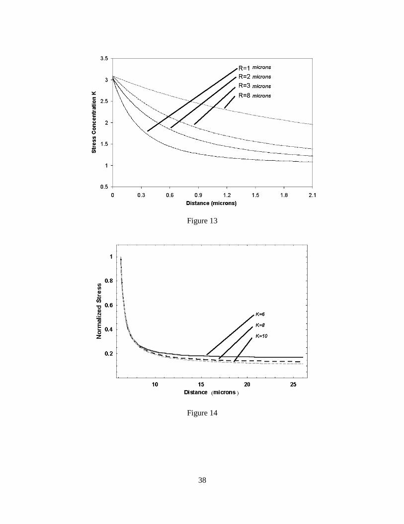
At the other extreme, consider the failure response under the maximum stress concentration for a

unit (micron) radius, but for variable stress intensities, which Figure 11 indicates to be about the

same. To explain this in terms of the statistical hypothesis we plot in Figure 13 the

circumferential (notch-tangential) stress for constant ρ = 1 micron, but for variable values of K=

6, 8, 10. Very close to the notch tip the stresses exhibit very nearly the same value and gradient

behavior, since the notch radii are the same. The important characteristic length scale that

influences the stress field near the root of the notch in this problem is clearly the radius of

curvature.

The dominating influence of the notch radius, and the accompanying size of the high-stress

region, is well summarized by the data in Figure 14. Although there is considerable scatter in the

data (see discussion on this point below) at least a tentative image emerges: The size of the high-

stress region is not sensitive to the notch radius, other than the circle (for small radii), regardless

of the stress concentration factor. Consequently the failure is governed (more or less) by the

domain size where high stresses reign. At a radius of one to three microns the failure data are not

particularly ordered according to the stress concentration factor. On the other hand, once the

notch radius attains large values on the order of eight to ten microns, Figure 13 indicates that a

25

difference in the stress level can become apparent for different stress concentration factors and,

consequently, the failure data in Figure 14 (see values at 10 microns) become ordered by the

stress concentration factor for the largest notch radius. Figure 14 also illustrates clearly the

(conservative) consequences of ignoring the size effect. The failure stresses resulting from small

notch radii are larger, on average, by a factor of about two than those derived from the large

scale (average) “property”.

In the previous discussion small-scale size effects have been demonstrated for the case of very

small notches. This behavior, however, could not be strictly isolated from the effect of the grain

size, which could not be varied for these experiments. To underscore the importance of the grain

structure, we include two tables (tables 1 and 2) that relate the geometry dimensions to the grain

size structure, as an additional means of relating these experiments to the very small scale.

In concluding this section it is worth pointing out that the size effect observed here should be

expected to be accompanied by increasing data scatter as the domain for failure occurrence

decreases. This observation is in agreement with all of our experimental results to date and

follows from the fact that flaws or defects are spatially distributed in the solid. Whether such a

flaw is enclosed in the high-stress region around a notch is thus a matter of probability. As this

region decreases, finding one or more “critical” flaws within it will become less deterministic,

and the failure behavior along with it: The statistics of the micro-structure play then an

increasingly important role.

26

5. Acknowledgements

The authors gratefully acknowledge the support by the Air Force Office of Scientific Research

through grant F49629-97-1-0324 (Round Robin Program), and under grant F49620-99-1-0091,

with Major Brian Sanders, Drs. O. Ochoa, D. Segalman and T. Hahn as the monitors.

6. References

Bruck, H.A., McNeil, S.R., Sutton, M.A., Peters, W.H., (1989). Digital image correlation using

Newton-Raphson method of partial differential correction. Exper. Mech., 29(3), 261-267.

Chasiotis, I., Knauss, W.G., (2000). Microtensile tests with the aid of probe microscopy for the

study of MEMS materials. Proc. of the Int. Soc. for Opt. Eng. (SPIE), 4175, 96-103.

Chasiotis I., Knauss W.G., 2001. The influence of fabrication governed surface conditions on the

mechanical strength of thin film materials. Proc. of the MRS, 657. 1-6.

Chasiotis I., Knauss W.G., 2002. A new microtensile tester for the study of MEMS materials

with the aid of atomic force microscopy. Exper. Mech. 42 (1), 1-7.

Huang, Y., (2001). Scanning tunneling microscopy and digital image correlation in

nanomechanics investigations. Ph.D. thesis, California Institute of Technology.

Isida, M., Nakagawa, K., (1954). On the stress gradients in tension and bending of a perforated

strip. Proc. of the third Japan Nat. Congress for Appl. Mech., 1-4.

Isida, M., (1955). On the tension of a strip with a central elliptic hole. Trans. of the Japan Soc.

of Mech. Eng., 21, 514.

Koester, D.A., Mahadevan, R., Hardy, B., Markus, K.W., (2000). MUMPs design handbook,

27

Rev. 5.0.

Luo, P.F., Chao, Y.J., Sutton, M.A., Peters, W.H., (1993). Accurate measurement of three-

dimensional deformations in deformable and rigid bodies using computer vision. Exp. Mech.,

50(2), 123-132.

Neuber, H., (1946). Theory of Notch Stresses. Edwards Bros Inc., Ann Arbor, Michigan, 1946.

Peters, W.H., Ranson, W.F., (1982). Digital image techniques in experimental stress analysis.

Opt. Eng., 21(3), 427-432.

Sutton, M.A., Wolters, W.J., Peters, W.H., Ranson, W.F., McNeil, S.R., (1983). Determination

of displacements using an improved digital image correlation method. Image Vision Comp.,

1(3), 133-139.

Sutton, M.A., Cheng, M., Peters, W.H., Chao, Y.J., McNeil, S.R., (1986). Application of an

optimized digital image correlation method to planar deformation analysis. Image Vision Comp.,

4(3), 143-150.

Tan, S.C., (1988). Finite width correction factors for anisotropic plate containing a central

opening. J. Comp. Mater., 22, 1080-1097.

Tsuchiya, T., Tabata, O., Sakata, J., Taga, Y., (1996). Tensile testing of polycrystalline silicon

thin films using electrostatic force grip. T.IEE Japan, 116-E(10), 441-446.

Vendroux, G., (1990). Correlation: A digital image correlation program for displacement and

displacement gradient measurements. GALCIT Report SM90-19, California Institute of

Technology.

Vendroux, G., Knauss, W.G., (1998). “Submicron deformation field measurements: part 2.

Improved digital image correlation. Exper. Mech., 38(2), 86-91.

28

FIGURE CAPTIONS

Figure 1. Terminology and illustration of one-dimensional image correlation.

Figure 2 Correlation error for a surface profile modeled by a square wave with an uncertainty

(imposed error) of εx=0.01, w=0.01+0.005x, iteration tolerance=10-5. Note that the abscissa

represents a nondimensional size scale.

Figure 3. Correlation error for inhomogeneous in-plane (in-line) straining of u=0.01x+0.001x2,

and zero out-of-plane deformation w=0, using only {u, du/dx} as parameters for minimization;

iteration tolerance=10-4.

Figure 4. Correlation error for the same inhomogeneous straining as for Figure 3,

u=0.01x+0.001x2, w=0, but with an additional parameter{u, du/dx, d2u/dx2} for minimization;

same iteration tolerance=10-4.

Figure 5. Line profiles taken from two consecutive scans along the same line. (a) Original signal,

(b) Filtered signal.

Figure 6. “Artificial” displacement produced from repetitive line scans.

Figure 7. Successive steps of film gripping.

Figure 8. Schematic of a die with 14 free-standing beams with various geometries.

Figure 9. SEM micrograph of elliptically perforated specimen.

Figure 10. SEM micrographs of perforations for nominal ρ=1 µm.

29

Figure 11. Geometry of the problem.

Figure 12. Local stress at failure for different stress concentrations. The gray bar indicates the

minimum recorded local strength and the white bar the scatter of the experimental data.

Figure 13. Stress concentration profile along the major axis of the ellipse for constant K and

different radius of curvature as calculated by the FEM model in ABAQUS.

Figure 14. Circumferential stress on y-axis as computed for different K and ρ=1 µm.

Figure 15. Experimental values of the average local failure stress as a function of the radius of

curvature.

30

FIGURES

F

oF

xo

~xo

f(x)

G

g(x)~oG

u(x)

xx

S

So

~x

Figure 1.

0 5 10 15 20-2

-1.5

-1

-0.5

0

0.5

1

1.5

2

2.5

3x 10-3

Correlation Points

Abs

olut

e E

rror

in U

subset=10subset=20subset=40subset=60subset=100

Figure 2

31

0.6 0.8 1 1.2 1.4 1.6 1.8 2 2.2-0.5

0

0.5

1

1.5

2

2.5x 10

-4

Correlation Points (µm)

Abs

olut

e E

rror

in U

subset=10subset=40subset=100subset=200

Figure 3

32

0.6 0.8 1 1.2 1.4 1.6 1.8 2 2.2-8

-6

-4

-2

0

2

4

6

8x 10

-5

Correlation Points (µm)

Abs

olut

e E

rror

in U

subset=10subset=40subset=100subset=200

Figure 4

33

0 1 2 3 4 5-10

-5

0

5

10

15

20z

(nm

)

0 1 2 3 4 5-10

-5

0

5

10

15

20

x (µm)

z (n

m)

(a)

(b)

Figure 5

34

50 100 150 200

-0.5

-0.4

-0.3

-0.2

-0.1

0

0.1

0.2

0.3

0.4

0.5

Correlation Points (pixel)

Dis

plac

emen

t u (p

ixel

)

Figure 6

35

Figure 7 Figure 8

Figure 9

2mm

36

K=3 K=6 K=8

Figure 10

Figure 11

37

Figure 12

38

Figure 13

Figure 14

39

Figure 15

40

TABLES

Table 1. Nominal K and dimensions of tested perforated specimens

Nominal K (Calculated for

infinite plate)

Radius of Curvature,

ρρρρ (µµµµm)

ρρρρ / d

(Notch radius) / (Grain

Size)

3 1, 2, 3, 8 3,6,10,25

6 1, 2, 3, 8 3,6,10,25

8 1, 2, 3, 8 3,6,10,25

Table 2. Stress gradient at the notch root and decay length for K=3

Radius of round notch

(µµµµm)

Stress gradient at y=ρρρρ

(GPa/µµµµm)

Characteristic length for

decay of stresses to σσσσf

1 -7.02 2 grains

2 -3.51 3 grains

3 -2.34 5 grains

8 -0.88 7 grains