mechanical engineering design ii · specify the lewis form factor for worm gear teeth from table...
TRANSCRIPT

Mechanical Engineering Design II
Twenty-two Lecture
Design of Worm Gear

Power Transmission Problem
Proposed solution(Worm Gear)
high velocity ratios in a single step in a minimum of spaceDesign Requirements
non-intersecting shafts at right angles
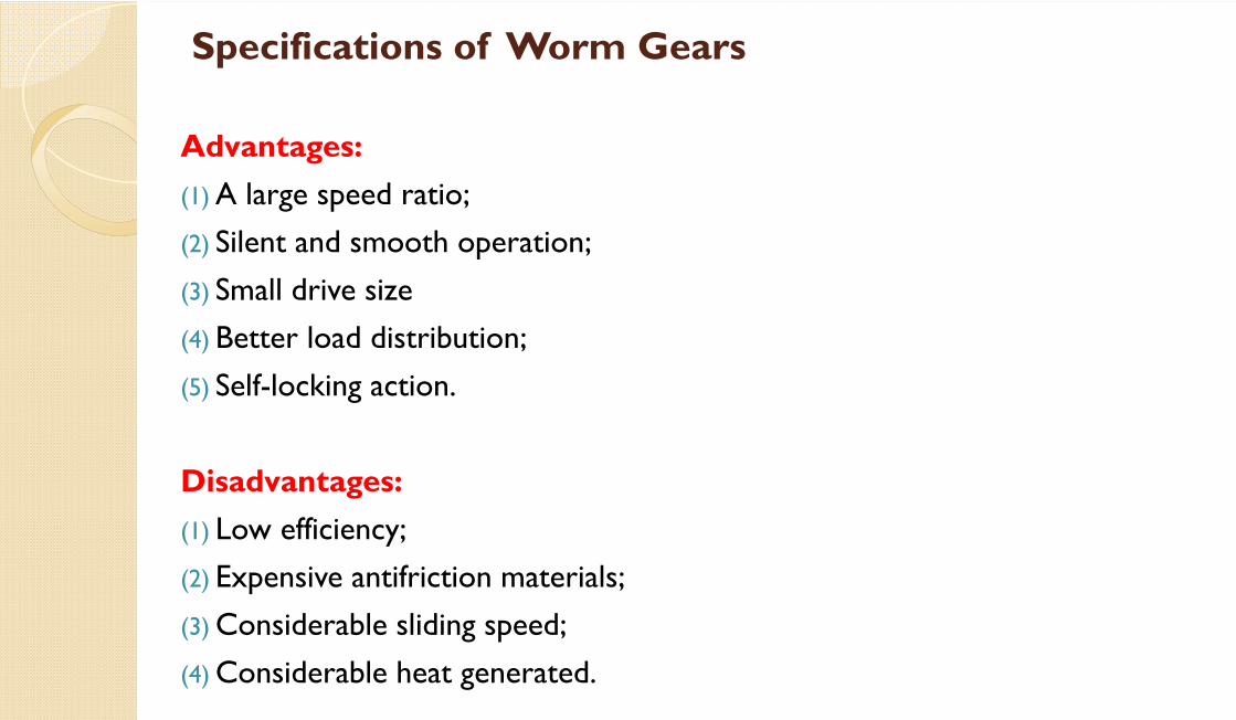
Specifications of Worm Gears
Advantages:(1) A large speed ratio;(2) Silent and smooth operation;(3) Small drive size(4) Better load distribution;(5) Self-locking action.
Disadvantages: (1) Low efficiency;(2) Expensive antifriction materials;(3) Considerable sliding speed;(4) Considerable heat generated.

Types of Worm Gears

Basic Worm Gear Geometry
DG = pitch diameter of the gear DW = pitch diameter of the worm NG = number of teeth in the gear NG = number of teeth in the wormC = center distance L = lead lead angle Px = axial pitchFG = Face width of gear Fw = Face length of the worm

Forces on Worm Gear
WtG = WxW
WxG = WtW
WrG = WrW
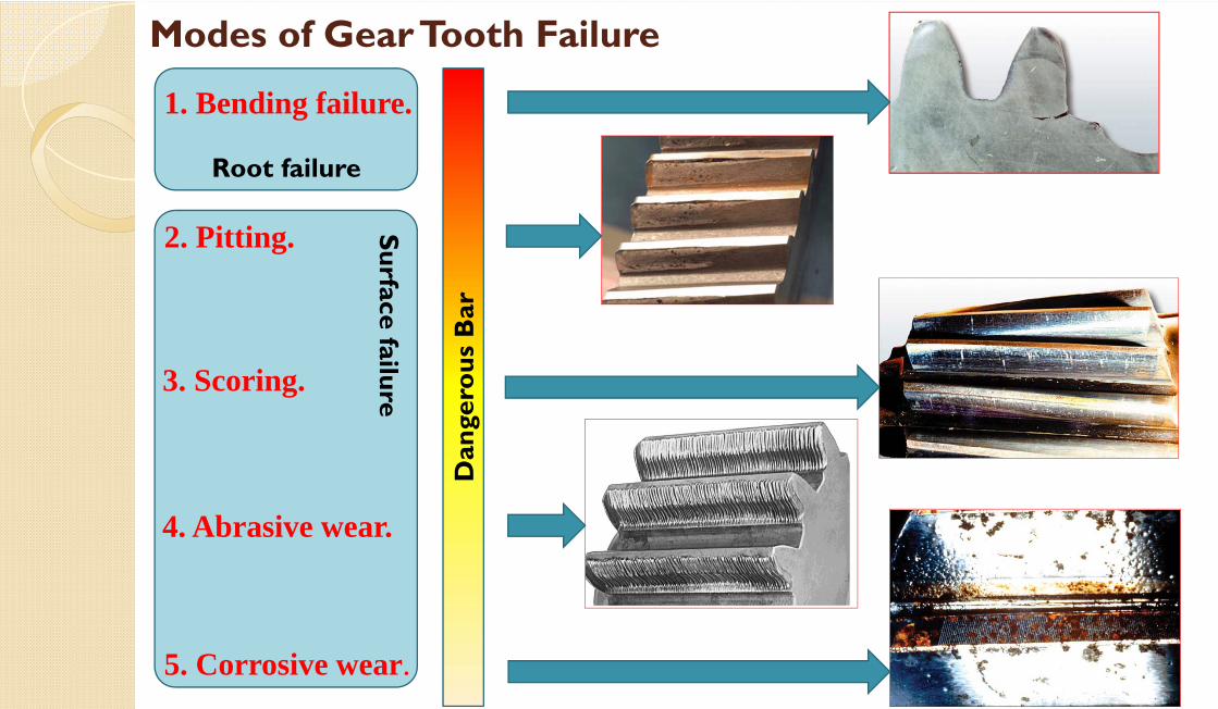
Surface failure
Root failure
Modes of Gear Tooth Failure
1. Bending failure.
2. Pitting.
3. Scoring.
4. Abrasive wear.
5. Corrosive wear.
Dan
gero
us B
ar

Worm Gear Design The power to be transmitted
The speed of the driving gear
The center distance
The speed of the driven gear or the velocity ratio
The gear teeth should not fail under static loading or dynamic loading during normal running conditions.
The use of space and material should be economical.
The alignment of the gears and deflections of the shafts must be considered.
The gear teeth should have wear characteristics so that their life is satisfactory.
The lubrication of the gears must be satisfactory.
Designer
Type of driver and driven load
Other information related to problem specification

Flowchart for worm gear designing process:
Transmitted Power , Input and Output speed, Center distance, Type of driver and driven load
1
Specify the no. of threads for Worm (from 2 to 8 or more)
Specify the diametral pitch (3 , 4 , 5 , 6 , 8 , 10 , 12 , 16 , 24 , 32 , 48)
Specify the Pressure angle (14.5o , 20o , 25o , 30o )
Compute the nominal velocity ratio
Compute the circular pitch for Gear ⁄ axial pitch for worm , normal circular pitch cos , and the
face width of gear
Compute the lead
Compute the pitch diameter of the worm within .
.
.

1
2
Compute the lead angle tan ⁄
Compute the pitch line speed of the worm and gear ,
Compute the sliding velocity sin⁄ cos⁄
Find the coefficient of friction from figure (10-18) page(477) (493pdf)
Compute the pitch diameter of gear ⁄

3
Compute the output torque ,
,
Friction force , Power loss / ,
Input Power ,
Efficiency
or from figure (10-19) page (479)
(495pdf)
2
3
4
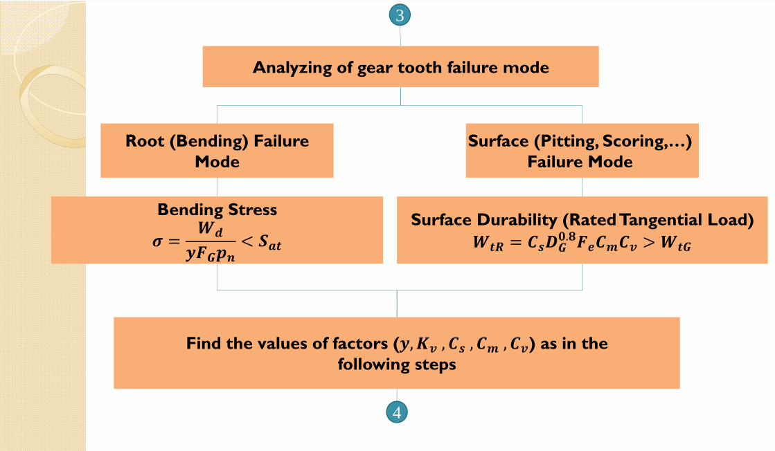
Root (Bending) Failure Mode
Analyzing of gear tooth failure mode
Surface (Pitting, Scoring,…) Failure Mode
Bending Stress Surface Durability (Rated Tangential Load).
Find the values of factors ( , , , , ) as in the following steps

Specify the Lewis form factor for worm gear teeth from Table (10-4) page(482) (Pdf 498)
4
5
Compute the dynamic load ⁄
Compute the dynamic load factor ⁄( in ft/min)

Specify the material factor ( ) from figure (10-20) page (483) (499pdf) or from the following equations:Sand-Casting Bronzes:
.. . log
.
Static-Chill-Cast or Forged Bronzes: .
. . log .
Centrifugally Cast Bronzes:
. . log
5
6
Note: if standard addendum gears are used,

6
Compute the effective face width in inches .
. .
7
Specify the Ratio correction factor from figure (10-21) page(484) (500pdf)
. . .
. .

7
Specify the velocity factor ( ) from figure(10-22) page (485) (501 pdf)
8
152 304 456 608 760 912 1064m/min
. .

8
Check if the selected dimensions satisfy the following design conditions:
First condition
, . ,
.
Second condition
Third condition
.


Mechanical Engineering Design II
Twenty-three Lecture
Introduction to Optimum Design

Design Optimization
stresses
noise
vibration
deflection
weight
cost
time
Undesirable effects
power transmitted
energy absorbed
overload capacity
factor of safety
Desirable effects
minim
izationm
axim
izat
ion


Init
ial d
esig
n
Final design


Method of Optimum Design, MOD
Sketching a model of the item to be designed
Functional Requirements Undesirable Effects
Reviewing the Boundary Conditions
Summarizing the Specifications and Constraints
Deriving the equations which tie the design variables together mathematically
Deriving the Primary Design Equation (P. D. E.)

The Basic Design Problem: Design a plastic tray capable of holding a specified volume of liquid, (V), such that the liquid has a specified depth of (H), and the wall thickness of the tray is to be a specified thickness, (T). The tray is to be in large quantities.

: Adequate Design Solution
∗ ∗ ………………… . 1
1. It is possible to know the value of (l) by choosing a value for (b).
2. It is possible to choose a certain type of material for the tray.
3. It is possible to choose an appropriate manufacturing method.
Since the tray is manufactured in large quantity, then:
1. The most significant undesirable effect for this problem is COST.
2. The objective of this design is to minimize COST.
Optimum Design Solution:
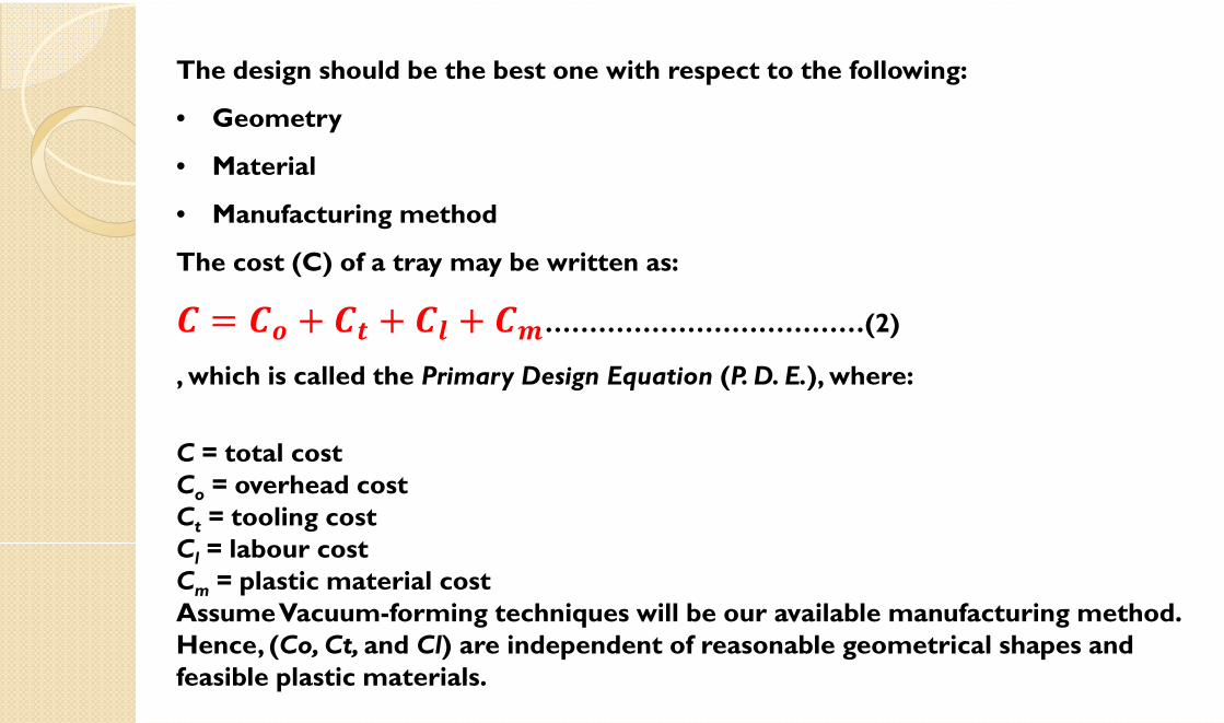
The design should be the best one with respect to the following:
• Geometry
• Material
• Manufacturing method
The cost (C) of a tray may be written as:
………………………………(2)
, which is called the Primary Design Equation (P. D. E.), where:
C = total cost Co = overhead cost Ct = tooling cost Cl = labour cost Cm = plastic material cost Assume Vacuum-forming techniques will be our available manufacturing method. Hence, (Co, Ct, and Cl) are independent of reasonable geometrical shapes and feasible plastic materials.

. . . . . . . …………………………
where: c = a unit volume of tray material, (ID / m3).
From equation (1) and equation (3a):
. . . . . ………………………………(3b)
. . . . . . .
∴
∴ .

Now, ∗ ∗
∴ ..
∴ . .
. . . .
………………………… . .

Optimum Design for Existing Restrictions: Let:
and

Mechanical Engineering Design II
Twenty-four & Twenty-five Lectures
Summary of Design Equations in Optimum Design

Typical Schematic Representation of Optimum Design:

Basic Procedural Steps for M.O.D.: Successive steps of a systematic plan lead to the specification of the optimum design, which is summarized as follows:
1. Initial Formulation, (I.F.): it is the summary of the initial system equations including (P.D, E.), (S.D.E.), and (L.E.)’s.
2. Final Formulation, (F.F.): it is a suitable transformation of (I.F.) for the use in the variation study step.
3. Variation Study, (V.S.): in this step, the (F.F.) equation system is considered simultaneously along with the Constraints for general determination of the point’s potential for Optimum Design. The sketching of Variation Diagram facilitates this step.
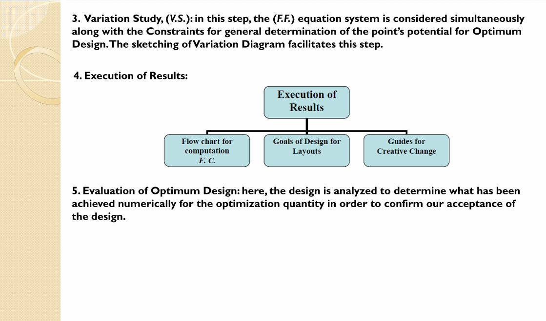
4. Execution of Results:
5. Evaluation of Optimum Design: here, the design is analyzed to determine what has been achieved numerically for the optimization quantity in order to confirm our acceptance of the design.

Types of Variables in I.F.:
• Constraints parameters in number, (nc), defined as the ones having either
regional constraints or discrete value, and directly imposed by (L.E.)’s in the
(I.F.).
• Free variables in number, (nf), defined as, the one with no constraints
directly imposed on them through (L.E.)’s in the (I.F.).
• Total number of the variables: nv = nc + nf

Types of Problems in M.O.D.: There are basically, three classes of problems encountered in application of (M.O.D.). They are summarized briefly below:
1. Case of Normal Specifications, N.S.: P.D.E. is single, often an independent material selection factor, (M.S.F.), is recognized. N.S. types of problems is: [nf >= Ns], where Ns = the number of (S.D.E.)’s.
2. Case of Redundant Specifications, R.S.: • Ignoring some of constraints on selected parameters that are called Eliminated
Parameters. • The P.D.E. designated as equation (Ι). • The Eliminated Parameters must be expressed by what is called as the relating
equations and designated as (ΙΙ, ΙΙΙ, ΙV, and so on), in (F.F.). • The test for the (R.S.) type problem is [nf < Ns].
3. Case of Incompatible Specifications: This is, in reality, nothing more than a special form of (R.S.). There is merely no design solution that satisfy all constraints, and speed. If boundary values changes, the domain of feasible design is opened and the optimum design can be determined by the (M.O.D.).

One of the most difficult details of execution lies in the transformation of the (I.F.) to (F.F.). Three general items are helpful in this respect. They will be outlined briefly below for the (R.S.) type of problem:
1. Exploratory Calculations: Dvs = nv – Ns + 1, where: Dvs =number of dimensions required for a (V.S.) , where: !
! !At = number of different approaches nc = number of constraints variables ne = number of eliminated parameters ne = Ns – nfnr = nc – ne, where: nr = number of related parameters.
2. Choosing the Approach: • Choice of the particular approach to take for derivation for the specific (F.F.), should be
made after thought. • Choose the simplest approach.
3.General Format of (F.F.): Summarizing the (F.F.) equations can be very helpful.
General Planning (I.F.) to (F.F.) in M.O.D.:

: Case of Normal Specifications )1Example (
Simple tensile bar, (mass production manufacturing)
L = specified length P = constant force Optimum design required to minimizing cost
• Now, the (P.D.E.) is: Cm = material cost =c.V = c.(A.L), where: Cm = cost of the bar material, c = unit volume material cost
• The undesirable effect are the stress =σ=P/A, which is the (S.D.E.).
• The limit equations are:
• Now, P, L and Ny are the Functional Requirements, • c & Sy are the Material Parameters, • A is the Geometrical Parameter, • σ &Cm are the Undesirable Parameters.
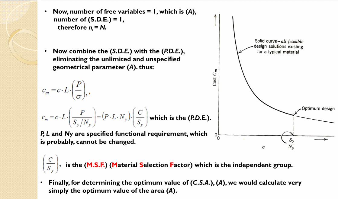
• Now, number of free variables = 1, which is (A), number of (S.D.E.) = 1,
therefore nf = Ns
• Now combine the (S.D.E.) with the (P.D.E.), eliminating the unlimited and unspecified geometrical parameter (A). thus:
which is the (P.D.E.).
P, L and Ny are specified functional requirement, which is probably, cannot be changed.
is the (M.S.F.) (Material Selection Factor) which is the independent group.
• Finally, for determining the optimum value of (C.S.A.), (A), we would calculate very simply the optimum value of the area (A).

Redundant Specifications : Case of )2Example (
Simple tensile bar, (mass production manufacturing), with:
Now, the (I.F.) is:
(P.D.E.)
(S.D.E.)
(L.E.)
(L.E.)
• In this case, it is impossible to combine (S.D.E.) with (P.D.E.). Now: nf = 0 and Ns =1
Therefore, the case is a Redundant Specification.
• There are two approaches: 1. Ignore the (S.D.E.) 2. Ignore the (L.E.), on stress or in (A).

Exploratory calculations: There are two approaches possible for (F.F.)’s. Our (V.S.) will be two dimensional in character.
• Say the simplest approach: σ is the eliminated parameter A is the related parameter.
The (F.F.) is the same as the (I.F.)
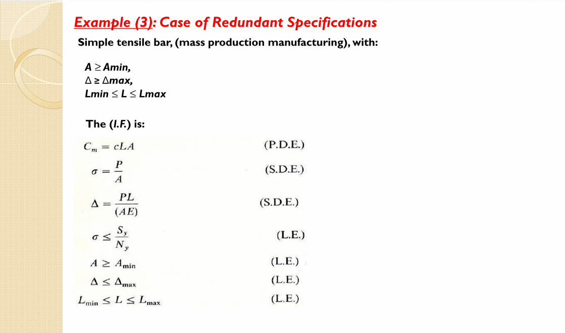
Redundant Specifications : Case of )3Example (Simple tensile bar, (mass production manufacturing), with:
A ≥ Amin, Δ ≥ Δmax, Lmin ≤ L ≤ Lmax
The (I.F.) is:

The (V.S.) are:
Therefore, the (F.F.) are:
