solutions MAnuAl FoR

by

Mechanical Design of Machine

coMponents

ansel c. UgURal

solutions MAnuAl FoR

by

Boca Raton London New York

CRC Press is an imprint of theTaylor & Francis Group, an informa business

Mechanical Design of Machine

coMponents

ansel c. UgURal

CRC PressTaylor & Francis Group6000 Broken Sound Parkway NW, Suite 300Boca Raton, FL 33487-2742

© 2015 by Taylor & Francis Group, LLCCRC Press is an imprint of Taylor & Francis Group, an Informa business

No claim to original U.S. Government works

Printed on acid-free paperVersion Date: 20141007

International Standard Book Number-13: 978-1-4398-9171-1 (Ancillary)

This book contains information obtained from authentic and highly regarded sources. Reasonable efforts have been made to publish reliable data and information, but the author and publisher cannot assume responsibility for the validity of all materials or the consequences of their use. The authors and publishers have attempted to trace the copyright holders of all material reproduced in this publication and apologize to copyright holders if permission to publish in this form has not been obtained. If any copyright material has not been acknowledged please write and let us know so we may rectify in any future reprint.

Except as permitted under U.S. Copyright Law, no part of this book may be reprinted, reproduced, transmitted, or utilized in any form by any electronic, mechanical, or other means, now known or hereafter invented, including photocopying, microfilming, and recording, or in any information storage or retrieval system, without written permission from the publishers.

For permission to photocopy or use material electronically from this work, please access www.copyright.com (http://www.copyright.com/) or contact the Copyright Clearance Center, Inc. (CCC), 222 Rosewood Drive, Danvers, MA 01923, 978-750-8400. CCC is a not-for-profit organization that provides licenses and registration for a variety of users. For organizations that have been granted a photocopy license by the CCC, a separate system of payment has been arranged.

Trademark Notice: Product or corporate names may be trademarks or registered trademarks, and are used only for identification and explanation without intent to infringe.

Visit the Taylor & Francis Web site athttp://www.taylorandfrancis.com

and the CRC Press Web site athttp://www.crcpress.com

vi

CONTENTS Section I BASICS Chapter 1 INTRODUCTION 1 Chapter 2 MATERIALS 16 Chapter 3 STRESS AND STRAIN 24 Chapter 4 DEFLECTION AND IMPACT 48 Chapter 5 ENERGY METHODS AND STABILITY 68 Section II FAILURE PREVENTION Chapter 6 STATIC FAILURE CRITERIA AND RELIABILITY 100 Chapter 7 FATIGUE FAILURE CRITERIA 117 Chapter 8 SURFACE FAILURE 135 Section III APPLICATIONS Chapter 9 SHAFTS AND ASSOCIATED PARTS 145 Chapter 10 BEARINGS AND LUBRICATION 164 Chapter 11 SPUR GEARS 176 Chapter 12 HELICAL, BEVEL, AND WORM GEARS 194 Chapter 13 BELTS, CHAINS, CLUTCHES, AND BRAKES 208 Chapter 14 MECHANICAL SPRINGS 225 Chapter 15 POWER SCREWS, FASTENERS, AND CONNECTIONS 240 Chapter 16 MISCELLANEOUS MECHANICAL COMPONENTS 261 Chapter 17 FINITE ELEMENT ANALYSIS IN DESIGN 278 Chapter 18 CASE STUDIES IN MACHINE DESIGN 308

vii

NOTES TO THE INSTRUCTOR The Solutions Manual to accompany the text Mechanical Design of Machine Components supplements the study of machine design developed in the book. The main objective of the manual is to provide efficient solutions for problems in design and analysis of variously loaded mechanical components. In addition, this manual can serve to guide the instructor in the assignment of problems, in grading these problems, and in preparing lecture materials as well as examination questions. Every effort has been made to have a solutions manual that cuts through the clutter and is self –explanatory as possible thus reducing the work on the instructor. It is written and class tested by the author.

As indicated in its preface, the text is designed for the junior-senior courses in machine or mechanical design. However, because of the number of optional sections which have been included, Mechanical Design of Machine Components may also be used to teach an upper level course. In order to accommodate courses of varying emphases, considerably more material has been presented in the book than can be covered effectively in a single three-credit-hour course. Machine/mechanical design is one of the student’s first courses in professional engineering, as distinct from basic science and mathematics. There is never enough time to discuss all of the required material in details.

The instructor has the choice of assigning problems using SI units and problems using U.S. customary units. To assist the instructor in making up a schedule that will best fit his classes, major topics that will probably be covered in every machine design course and secondary topics which may be selected to complement this core to form courses of various emphases are indicated in the following Sample Assignment Schedule. The major topics should be covered in some depth. The secondary topics, because of time limitations and/or treatment on other courses, are suggested for brief coverage. We note that the topics which may be used with more advanced students are marked with asterisks in the textbook.

The problems in the sample schedule have been listed according to the portions of material they

illustrate. Instructor will easily find additional problems in the text to amplify a particular subject in discussing a problem assigned for homework. Answers to selected problems are given at the end of the text. Space limitations preclude our including solutions to open-ended web problems. Since the integrated approach used in this text differs from that used in other texts, the instructor is advised to read its preface, where the author has outlined his general philosophy. A brief description of the topics covered in each chapter throughout the text is given in the following. It is hoped that this material will help the instructor in organizing his course to best fit the needs of, his students. Ansel C. Ugural Holmdel, N.J.

viii

DESCRIPTION OF THE MATERIAL CONTAINED IN “Mechanical Design of Machine Components”

Chapter 1 attempts to present the basic concepts and an overview of the subject. Sections 1.1 through 1.8 discuss the scope of treatment, machine and mechanical design, problem formulation, factor of safety, and units. The load analysis is normally the critical step in designing any machine or structural member (Secs. 1.8 through 1.9). The determination of loads is encountered repeatedly in subsequent chapters. Case studies provide a number of machine or component projects throughout the book. These show that the members must function in combination to produce a useful device. Section 1.10 review the work, energy, and power. The foregoing basic considerations need to be understood in order to appreciate the loading applied to a member. The last two sections emphasize the fact that stress and strain are concepts of great importance to a comprehension of design analysis.

Chapter 2 reviews the general properties of materials and some processes to improve the strength of metals. Sections 2.3 through 2.14 introduce stress-strain relationships, material behavior under various loads, modulus of resilience and toughness, and hardness, selecting materials. Since students have previously taken materials courses, little time can be justified in covering this chapter. Much of the material included in Chapters 3 through 5 is also a review for students. Of particular significance are the Mohr’s circle representation of state of stress, a clear understanding of the three-dimensional aspects of stress, influence of impact force on stress and deformation within a component, applications of Castigliano’s theorem, energy of distortion, and Euler’s formula. Stress concentration is introduced in here, but little applications made of it until studying fatigue (Chap.7).

The first section of Chapter 6 attempts to provide an overview of the broad subject of “failure”, against which all machine/mechanical elements must be designed. The discipline of fracture mechanics is introduced in Secs. 6.2 through 6.4. Yield and fracture criteria for static failure are discussed in Secs. 6.4 through 6.12. The last 3 sections deal with the method of reliability prediction in design. Chapter 7 is devoted to the fatigue and behavior of materials under repeated loadings. The emphasis is on the Goodman failure criterion. Surface failure is discussed in Chapter 8. Sections 8.1 through 8.3 briefly review the corrosion and friction. Following these the surface wear is discussed. Sections 8.6 through 8.10 deal with the surfaces contact stresses and the surface fatigue failure and its prevention. The background provided here is directly applied to representative common machine elements in later chapters.

Sections 9.1 through 9.4 of Chapter 9 treat the stresses and design of shafts under static loads.

Emphasis is on design of shafts for fluctuating loading (Secs. 9.6 and 9.7). The last 5 sections introduce common parts associated with shafting. Chapter 10 introduces the lubrication as well as both journal and roller bearings. As pointed out in Sec. 8.9, rolling element bearings provide interesting applications of contact stress and fatigue. Much of the material covered in Secs. 11.1 through 11.7 of Chapter 11 deal with nomenclature, tooth systems, and fundamentals of general gearing. Gear trains and spur gear force analysis are taken up in Secs. 11.6 and 11.7. The remaining sections concern with gear design, material, and manufacture. Non-spur gearing is considered in Chapter 12. Spur gears are merely a special case of helical gears (Secs. 12.2 through 12.5) having zero helix angle. Sections 12.6 through 12.8 deal with bevel gears. Worm gears are fundamentally different from other gears, but have much in common with power screws to be taken up in Chap. 15.

ix

Chapter 13 is devoted to the design of belts, chains, clutches, and brakes. Only a few different analyses are needed, with surface forms effecting the equations more than the functions of these devices. Belts, clutches, and brakes are machine elements depending upon friction for their function. Design of various springs is considered in Chapter 14. The emphasis is on helical coil springs (Secs. 14.3 through 14.9) that provide good illustrations of the static load analysis and torsional fatigue loading. Leaf springs (Sec. 14.11) illustrate primarily bending fatigue loading. Chapter 15 attempts to present screws and connections. Of particular importance is the load analysis of power screws and a clear understanding of the fatigue stresses in threaded fasteners. There are alternatives to threaded fasteners and riveted or welded joints. Modern adhesives (Secs. 15.17 and 15.18) can change traditional preferred choices.

It is important to assign at least portions of the analysis and design of miscellaneous mechanical members treated in Chapter 16. Sections 16.3 through 16.7 concern with thick-walled cylinders, press or shrink fits, and disk flywheels. The remaining sections introduce the bending of curved frames, plate and shells-like machine and structural components, and pressure vessels. Buckling of thin-walled cylinders and spheres is also briefly discussed. Chapter 17 represents an addition to the material traditionally covered in “Machine/Mechanical Design” textbooks. It attempts to provide a comprehensive introduction to the finite element analysis in mechanical design. A variety of case studies illustrate solutions of problems involving structural assemblies, stress concentration factors in plates and disks, and thick-walled pressure vessels. Finally, case studies in preliminary design of the entire crane with winch and a high-speed cutting machine are introduced in Chapter 18.

x

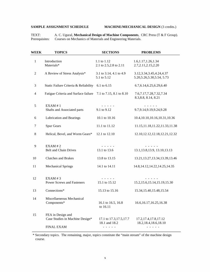
SAMPLE ASSIGNMENT SCHEDULE MACHINE/MECHANICAL DESIGN (3 credits.) TEXT: A. C. Ugural, Mechanical Design of Machine Components, CRC Press (T & F Group). Prerequisites: Courses on Mechanics of Materials and Engineering Materials.

WEEK TOPICS SECTIONS PROBLEMS 1 Introduction 1.1 to 1.12 1.6,1.17,1.26,1.34 Materials* 2.1 to 2.5,2.8 to 2.11 2.7,2.11,2.15,2.20 2 A Review of Stress Analysis* 3.1 to 3.14, 4.1 to 4.9 3.12,3.34,3.45,4.24,4.37 5.1 to 5.12 5.20,5.26,5.30,5.54, 5.73 3 Static Failure Criteria & Reliability 6.1 to 6.15 6.7,6.14,6.25,6.29,6.40 4 Fatigue Criteria and Surface failure 7.1 to 7.15, 8.1 to 8.10 7.6,7.17,7.28,7.32,7.34 8.3,8.8, 8.14, 8.21 5 EXAM # 1 - - - - - - - - - - Shafts and Associated parts 9.1 to 9.12 9.7,9.14,9.19,9.24,9.28 6 Lubrication and Bearings 10.1 to 10.16 10.4,10.10,10.16,10.31,10.36 7 Spur Gears 11.1 to 11.12 11.15,11.18,11.22,11.33,11.38 8 Helical, Bevel, and Worm Gears* 12.1 to 12.10 12.10,12.12,12.18,12.21,12.32 9 EXAM # 2 - - - - - - - - - - Belt and Chain Drives 13.1 to 13.6 13.1,13.8,13.9, 13.10,13.13 10 Clutches and Brakes 13.8 to 13.15 13.21,13.27,13.34,13.39,13.46 11 Mechanical Springs 14.1 to 14.11 14.8,14.12,14.22,14.25,14.35 12 EXAM # 3 - - - - - - - - - - Power Screws and Fasteners 15.1 to 15.12 15.2,15.6,15.14,15.19,15.30 13 Connections* 15.13 to 15.16 15.34,15.40,15.48,15.54 14 Miscellaeneous Mechanical Components* 16.1 to 16.5, 16.8 16.6,16.17,16.25,16.38 to 16.11 15 FEA in Design and Case Studies in Machine Design* 17.1 to 17.3,17.5,17.7 17.2,17.4,17.8,17.12

18.1 and 18.2 18.2,18.4,18.6,18.10 FINAL EXAM - - - - - - - - - - * Secondary topics. The remaining, major, topics constitute the “main stream” of the machine design course.

1

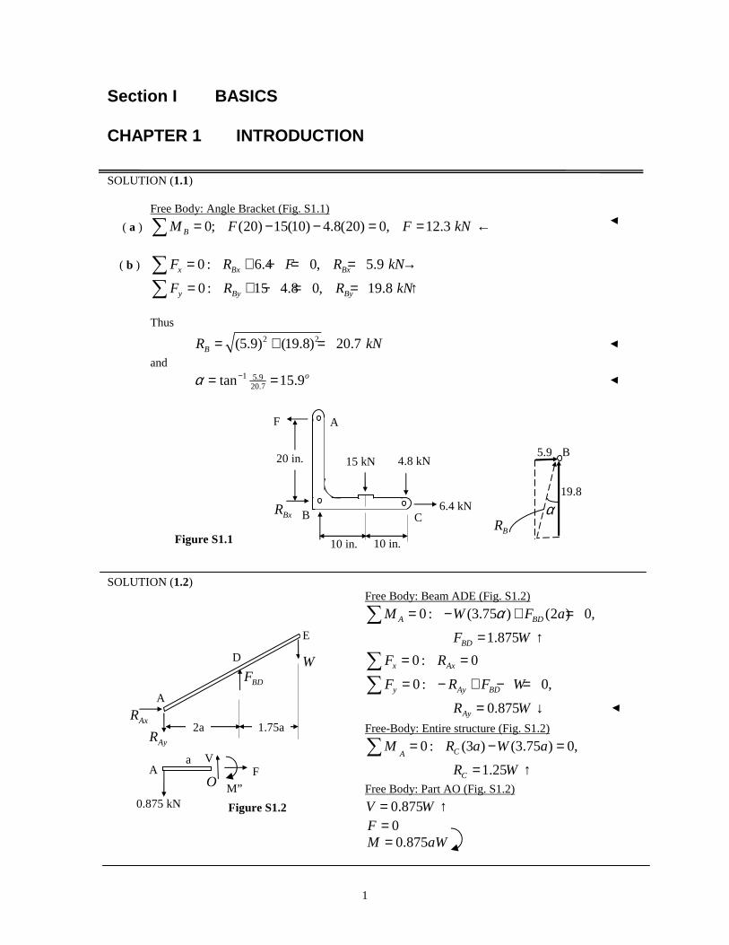
Section I BASICS CHAPTER 1 INTRODUCTION SOLUTION (1.1) Free Body: Angle Bracket (Fig. S1.1)

( a ) 0; (20) 15(10) 4.8(20) 0, 12.3BM F F kN= − − = = ←∑

( b ) 0 : 6.4 0, 5.9x Bx BxF R F R kN= + − = = →∑

0 : 15 4.8 0, 19.8y By ByF R R kN= + − = = ↑∑

Thus

2 2(5.9) (19.8) 20.7BR kN= + =

and

1 5.920.7tan 15.9oα −= =

SOLUTION (1.2) Free Body: Beam ADE (Fig. S1.2)

0 : (3.75 ) (2 ) 0,A BDM W F aα= − + =∑

1.875BDF W= ↑

0 : 0x AxF R= =∑

0 : 0,y Ay BDF R F W= − + − =∑

0.875AyR W= ↓

Free-Body: Entire structure (Fig. S1.2)

0 : (3 ) (3.75 ) 0,CAM R a W a= − =∑

1.25CR W= ↑

Free Body: Part AO (Fig. S1.2)

0.875V W= ↑

0F =

0.875M aW=

BDF

M”

A

0.875 kN

D

A

V F

O

E

W

Figure S1.2

2a 1.75a

a

AxR

AyR

α

B

19.8

5.9

BR Figure S1.1

15 kN

C

A F

6.4 kN

10 in.

4.8 kN

BxR

10 in.

20 in.

B

2

SOLUTION (1.3)

M R kipsA B= = ↓∑ 0 2 5: .

F R kipsy A= = ↑∑ 0 10 5: .

Segment CD

M kip ftD = = ⋅12

22 2 4( )( )

V kipsD = 4

Segment CE M kip ftE = − = ⋅8 6 105 4 6( ) . ( )

V kipsE = 25.

SOLUTION (1.4)

( a ) M R RB C C∑ = − − =0 08 6 0 6 2 24 4 0: . ( ) . ( ) ( )

∴ =R kNC 26 667.

R kN R kNCx Cy= =16 21334, .

Then

F R kNx Bx∑ = =0 16:

F R kNy By∑ = =0 12 66: .

( b ) Segment CD M kN mD = − − = ⋅21334 3 12 15 6 2 34. ( ) ( . ) ( )

F kND = 16

V kND = − =21334 18 3334. .

C 2’

4’ 4’ E

kips8

105. A

VE

M E

FD

M D 4

8

C

16

3 m D VD 21.334

C B A E D

RB RA 4’

2’

8’ 8’

24 kip ft⋅ 2 kip/ft

C D 2’

M D

VD

2 kip/ft

1 m 2m

3m D

RBy

A

RC

8 kN m

10 kN

RBx 4

3

B 2 m

2 m

C

3

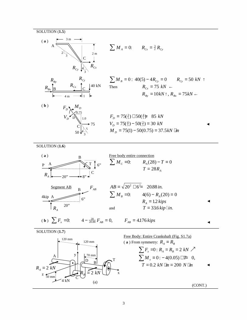
SOLUTION (1.5) ( a )

M R RA Cx Cy∑ = =0 32:

↑==−=∑ kNRRM CyCyB 5004)5(40:0

Then R kNCx = ←75

←=↑= kNRkNR BxBy 75,10

( b )

F kND = + =75 50 8535

45( ) ( )

V kND = − =75 50 3045

35( ) ( )

mkNM D ⋅=−= 5.37)75.0(50)1(75

SOLUTION (1.6) ( a ) Free body entire connection

M R TC A= − =∑ 0 28 0: ( )

T RA= 28

Segment AB AB in= + =20 6 20882 2 . .

M RB A= − =∑ 0 4 6 20 0: ( ) ( )

R kipsA = 12.

and T kip in= ⋅336. .

( b ) F F F kipsx AB AB= − = =∑ 0 4 0 41762020 88: , ..

SOLUTION (1.7) Free Body: Entire Crankshaft (Fig. S1.7a)

( a ) From symmetry: A BR R=

0 : 2z A BF R R kN= = =∑ ր

0 : 4(0.05) 0,xM T= − + =∑

0.2 200T kN m N m= ⋅ = ⋅

(CONT.)

RA

FAB

20”

6” 4kip

B

A

RA

P A

B

T 6”

20” 8” C

FD M D

VD D

4 3 50

75

0.75

1.0

C 5

RBy

RBx B RCx 40 kN

C

4 3

RCy

A

C

RCx

3 m

2 m 2 3

4 m 1 m

CyR

kNRB 2=

B

4 kN C 50 mm

A D

120 mm 120 mm

70 mm

2AR kN=

z

y T

x

(a)

4

1.7 (CONT.) ( b ) Cross Section at D (Fig. S1.7b)

2zV kN= ր

200T N m= ⋅

2(0.07) 0.14yM kN m= = ⋅

140 N m= ⋅

SOLUTION (1.8) Free-Body Diagram, Beam AB

765

0 : 60 0, 69.11x CD CDF F F kN= − + = =∑

465

0 : 30 0, 64.3y A CD AF R F R kN= − − = = ↑∑

765

0 : 60(1.8) (3) 0,A CD AM F M= − + − =∑

72AM kN m= ⋅

SOLUTION (1.9) Free body entire frame

M R RA Dy Dy= − − + =∑ 0 30 3 4 10 012: ( ) ( ) ( )

R kips R kipsDy Dx= =1125 5625. , .

Free body BCD

F R kipsx Bx= =∑ 0 5625: .

F R kipsy By= =∑ 0 1125: .

R kipsB = + =5625 1125 12 582 2. . .

B

8’ 4’

C

11.25

5.625 D

RBx

RBy

A

B C

D

30 kips 3’ 3’ 4’

1 2

4’

8’

RDy RD

12 RDy

CDF

A

30 kN

C

60 kN

B

4 7

ARAM

1.8 m

1.8 m

1.2 m

Figure S 1.7

zV

yM

T

D

(b)

5

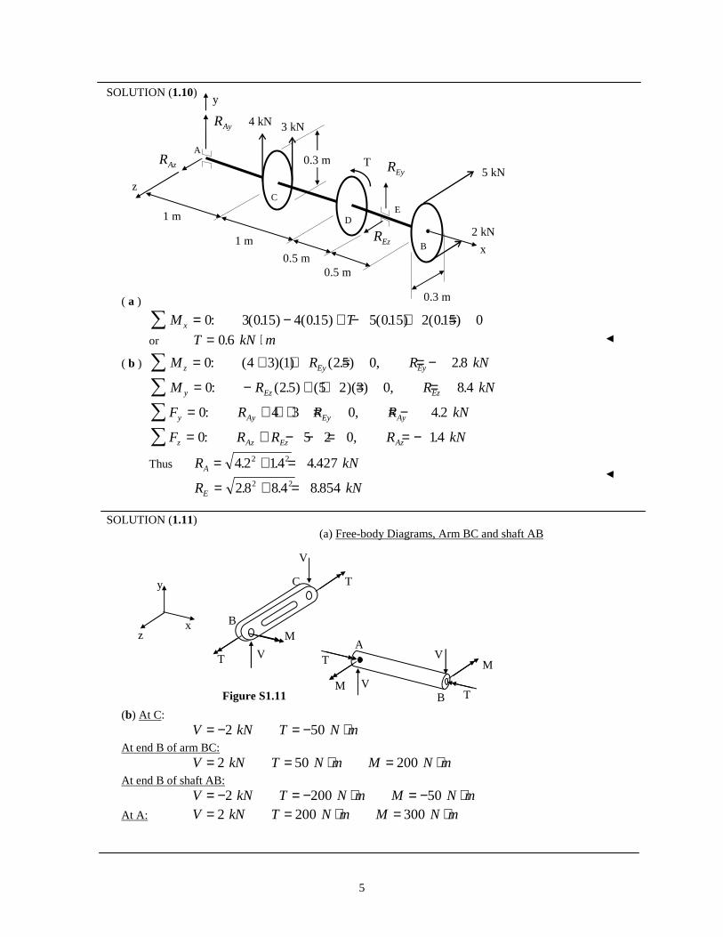
SOLUTION (1.10) ( a )

M Tx∑ = − + − + =0 3 015 4 015 5 015 2 015 0: ( . ) ( . ) ( . ) ( . )

or T kN m= ⋅0 6.

( b ) M R R kNz Ey Ey∑ = + + = = −0 4 3 1 25 0 28: ( )( ) ( . ) , .

M R R kNy Ez Ez= − + + = =∑ 0 25 5 2 3 0 8 4: ( . ) ( )( ) , .

F R R R kNy Ay Ey Ay∑ = + + + = = −0 4 3 0 4 2: , .

F R R R kNz Az Ez Az∑ = + − − = = −0 5 2 0 14: , .

Thus R kNA = + =4 2 14 4 4272 2. . .

R kNE = + =28 8 4 8 8542 2. . .

SOLUTION (1.11) (a) Free-body Diagrams, Arm BC and shaft AB (b) At C: 2 50V kN T N m= − = − ⋅

At end B of arm BC: 2 50 200V kN T N m M N m= = ⋅ = ⋅

At end B of shaft AB: 2 200 50V kN T N m M N m= − = − ⋅ = − ⋅

At A: 2 200 300V kN T N m M N m= = ⋅ = ⋅

C

D

B

E

A

z

RAz

RAy

y

x

T REy

REz

5 kN

2 kN

4 kN 3 kN

0.3 m

1 m

1 m

0.5 m 0.5 m

0.3 m

B

C

A

V

T

z

y

x

V

V M

M

T

T

M

T

B Figure S1.11

V

6

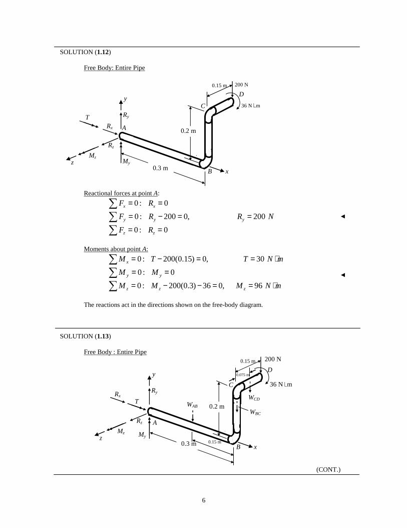
SOLUTION (1.12)

Free Body: Entire Pipe

Reactional forces at point A:

0 : 0x xF R= =∑

0 : 200 0, 200y y yF R R N= − = =∑

0 : 0z zF R= =∑

Moments about point A:

0 : 200(0.15) 0, 30xM T T N m= − = = ⋅∑

0 : 0y yM M= =∑

0 : 200(0.3) 36 0, 96z z zM M M N m= − − = = ⋅∑

The reactions act in the directions shown on the free-body diagram.

SOLUTION (1.13) Free Body : Entire Pipe (CONT.)

T

z

Rz

Ry

x

Mz

Rx

D

B

My

A

C y

0.15 m

0.3 m

0.2 m

200 N

36 N⋅ m

T

z

Rz

Ry

x

Mz

Rx

D

B

My

A

200 N

C 36 N⋅ m

y

0.15 m

0.3 m

0.2 m WCD

WAB WBC

0.075 m

0.15 m

7

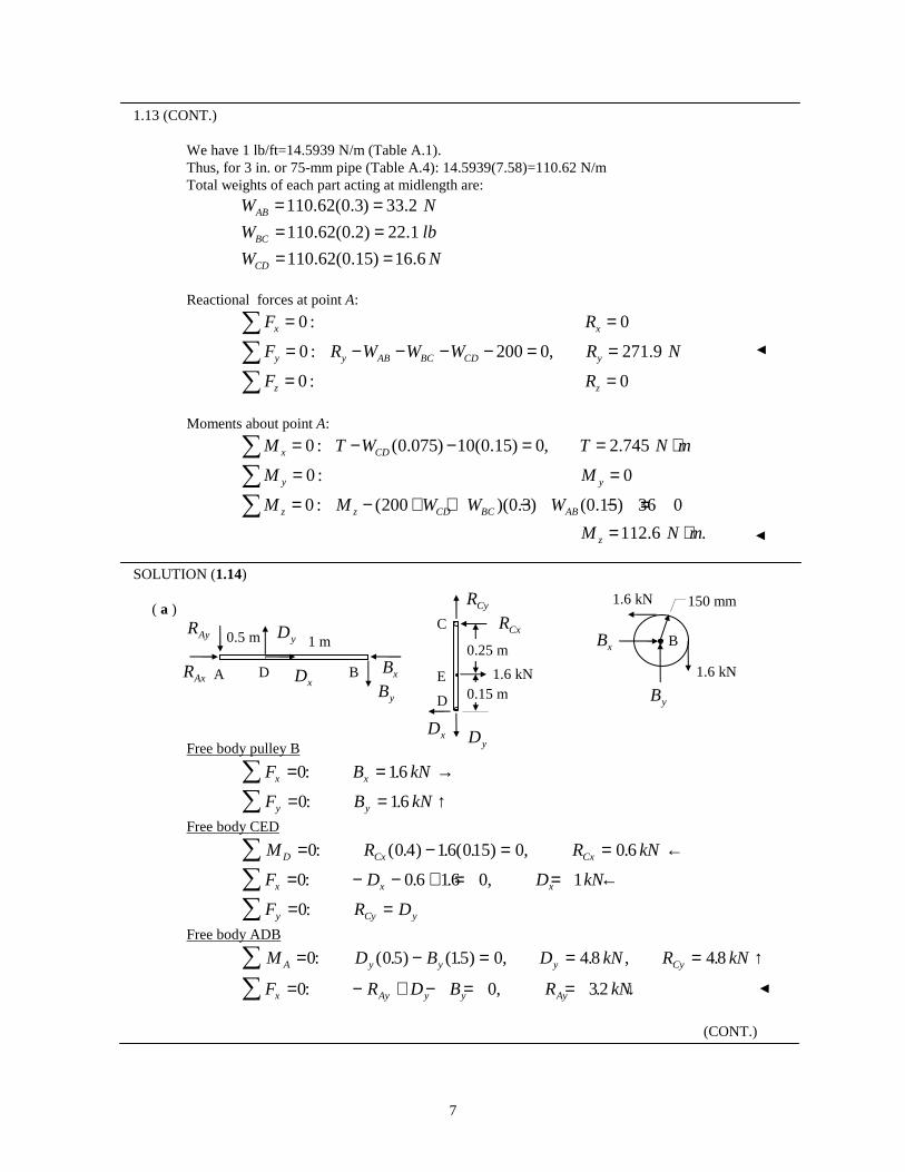
1.13 (CONT.) We have 1 lb/ft=14.5939 N/m (Table A.1). Thus, for 3 in. or 75-mm pipe (Table A.4): 14.5939(7.58)=110.62 N/m

Total weights of each part acting at midlength are:

110.62(0.3) 33.2ABW N= =

110.62(0.2) 22.1BCW lb= =

110.62(0.15) 16.6CDW N= =

Reactional forces at point A:

0 :xF =∑ 0xR =

0 : 200 0, 271.9y y AB BC CD yF R W W W R N= − − − − = =∑

0 :zF =∑ 0zR =

Moments about point A:

0 : (0.075) 10(0.15) 0, 2.745x CDM T W T N m= − − = = ⋅∑

0 :yM =∑ 0yM =

0 : (200 )(0.3) (0.15) 36 0z z CD BC ABM M W W W= − + + − − =∑

112.6 .zM N m= ⋅

SOLUTION (1.14) ( a ) Free body pulley B

F B kNx x= = →∑ 0 16: .

F B kNy y= = ↑∑ 0 16: .

Free body CED

M R R kND Cx Cx= − = = ←∑ 0 0 4 16 015 0 0 6: ( . ) . ( . ) , .

F D D kNx x x= − − + = = ←∑ 0 0 6 16 0 1: . . ,

F R Dy Cy y= =∑ 0:

Free body ADB

M D B D kN R kNA y y y Cy= − = = = ↑∑ 0 05 15 0 4 8 48: ( . ) ( . ) , . , .

F R D B R kNx Ay y y Ay= − + − = = ↓∑ 0 0 32: , .

(CONT.)

A

RAy

RAx

Dy

Dx D B By

Bx

1 m 0.5 m C

E

D

Dx Dy

0.25 m

0.15 m

RCy

RCx

1.6 kN

Bx

By

B

1.6 kN 150 mm

1.6 kN

8

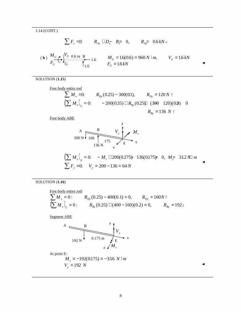
1.14 (CONT.)

F R D B R kNx Ax x x Ax= + − = = →∑ 0 0 0 6: , .

( b ) M N m V kNG G= = ⋅ =16 0 6 960 16. ( . ) , .

F kNG = 16.

SOLUTION (1.15) Free body entire rod

M R R Nx Dy Dy= − = ↑∑ 0 0 25 300 01 120: ( . ) ( . ),

( )M Rz C By∑ = − + + − =0 200 035 0 25 300 120 0 2 0: ( . ) ( . ) ( )( . )

R NBy = ↑136

Free body ABE

( )M M M N mz E z z∑ = − + − = = ⋅0 200 0 275 136 0175 0 312: ( . ) ( . ) , .

F V Ny y= = − =∑ 0 200 136 64:

SOLUTION (1.16) Free body entire rod:

↑==−=∑ NRRM DyDyx 160,0)1.0(400)25.0(:0

( ) ↓==−+=∑ 192,0)2.0)(160400()25.0(:0 ByByCz RRM

Segment ABE At point E: M N mz = − = − ⋅192 0175 336( . ) .

V Ny = 192

B 1.6

1.6 G

VG 0.6 m MG

FG

E

y

z x

M z Vy B A

200 N

136 N

100 175

A B y

x

z

E 192 N M z

Vy

0.175 m

9

SOLUTION (1.17) Side view Top view

Fig. (b): M F F kNA∑ = − = =0 0 05 150 0 31 1: ( . ) ,

Fig. (a): M F F F kNB∑ = − = =0 01 0 05 0 61 2 2: ( . ) ( . ) ,

Fig. (c): mkNTTFM ddD ⋅==−=∑ 3.0,0)05.0(:0 2

SOLUTION (1.18) Free body-entire frame

M R R kipsA y y∑ = − − = =0 30 3 18 4 12 0 34: ( ) ( ) ( ) , .

Free body-member BC

M R RC x y∑ = − =0 9 12 0: ( ) ( )

and

R kipsx = =43 34 4 533( . ) .

Thus

F R kipsBC = = + =( . ) ( . ) .4533 34 56662 2

B C

50 mm

100 mm

D

50 mm

A 50 mm

F2

F2

F1

F1

Td

N m⋅ 150

Figure (a) Figure (c)

Figure (b)

C

B

A 4

3

Rx Ry

R

4 kips 3 kips

12 ft 18 ft

9 ft

3ft

10

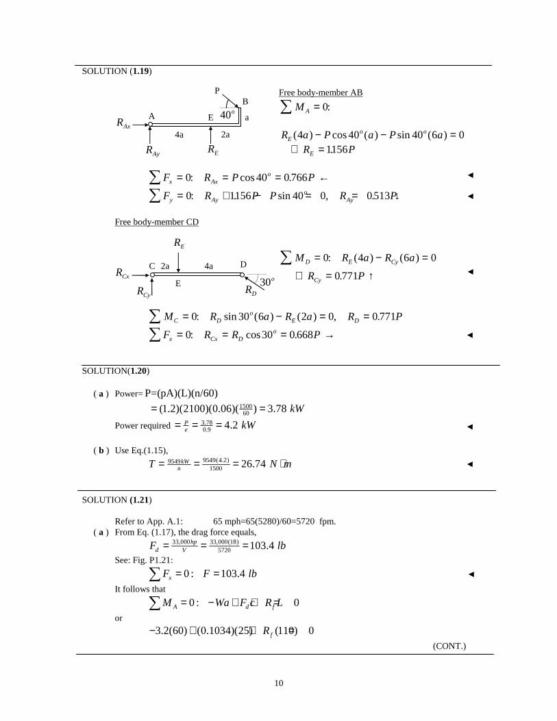
SOLUTION (1.19) Free body-member AB

M A∑ = 0:

R a P a P aEo o( ) cos ( ) sin ( )4 40 40 6 0− − =

∴ =R PE 1156.

F R P Px Axo= = = ←∑ 0 40 0 766: cos .

F R P P R Py Ayo

Ay= + − = = ↓∑ 0 1156 40 0 0513: . sin , .

Free body-member CD

M R a R aD E Cy= − =∑ 0 4 6 0: ( ) ( )

∴ = ↑R PCy 0 771.

M R a R a R PC Do

E D= − = =∑ 0 30 6 2 0 0 771: sin ( ) ( ) , .

F R R Px Cx Do∑ = = = →0 30 0 668: cos .

SOLUTION(1.20) ( a ) Power=P=(pA)(L)(n/60)

150060(1.2)(2100)(0.06)( ) 3.78kW= =

Power required 3.780.9 4.2P

e kW= = =

( b ) Use Eq.(1.15),

9549(4.2)9549

1500 26.74kWnT N m= = = ⋅

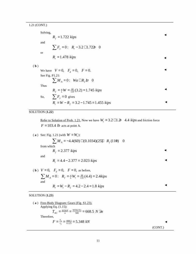
SOLUTION (1.21) Refer to App. A.1: 65 mph=65(5280)/60=5720 fpm. ( a ) From Eq. (1.17), the drag force equals,

33,000 33,000(18)

5720 103.4hpd VF lb= = =

See: Fig. P1.21:

0 : 103.4xF F lb= =∑

It follows that

0 : 0A d fM Wa F c R L= − + + =∑

or

3.2(60) (0.1034)(25) (110) 0fR− + + =

(CONT.)

C D

E

2a 4a RCx

RCy

RE

RD 30o

P B

a 40o A RAx

RAy RE

4a 2a

E

11

1.21 (CONT.) Solving,

1.722fR kips=

and

0 : 3.2 1.722 0y rF R= − + =∑

or

1.478rR kips=

( b )

We have 0, 0, 0.dV F F= = =

See Fig. P1.21:

0 : 0A fM Wa R L= + =∑

Thus

60110 (3.2) 1.745a

f LR W kips= = =

So, 0yF =∑ gives

3.2 1.745 1.455r fR W R kips= − = − =

SOLUTION (1.22)

Refer to Solution of Prob. 1.21. Now we have 3.2 1.2 4.4tW kips= + = and friction force

103.4F lb= acts at point A.

( a ) See: Fig. 1.21 (with tW W= ):

4.4(60) (0.1034)(25) (110) 0A fM R= − + + =∑

from which

2.377fR kips=

and

4.4 2.377 2.023rR kips= − =

( b ) 0, 0, 0,dV F F= = = as before,

601100 : (4.4) 2.4a

A f tLM R W kips= = = =∑

and

4.2 2.4 1.8r t fR W R kips= − = − =

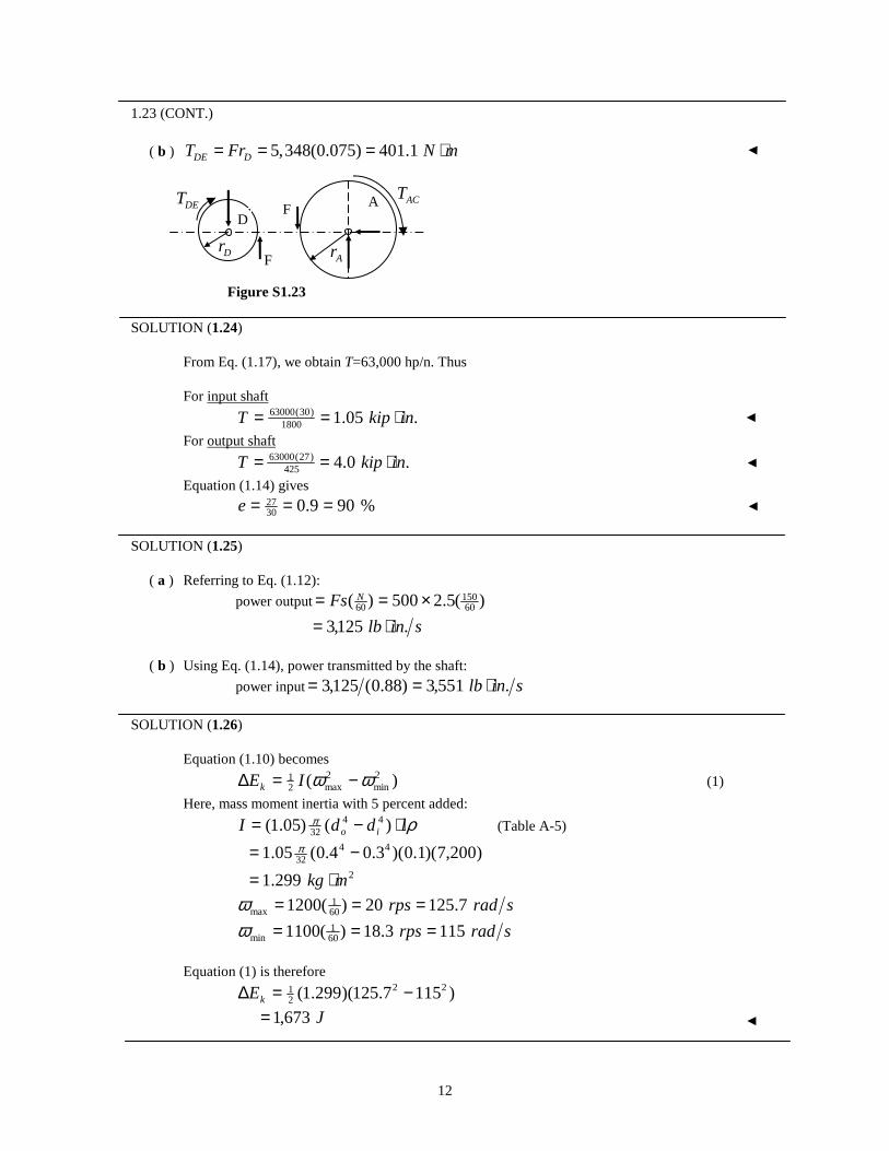
SOLUTION (1.23) ( a ) Free-Body Diagram: Gears (Fig. S1.23). Applying Eq. (1.15):

9550(35)9550

500 668.5PAC nT N m= = = ⋅

Therefore,

668.50.125 5.348A

A

TrF kN= = =

(CONT.)

12

1.23 (CONT.)

( b ) 5,348(0.075) 401.1DE DT Fr N m= = = ⋅

SOLUTION (1.24) From Eq. (1.17), we obtain T=63,000 hp/n. Thus For input shaft

.05.11800)30(63000 inkipT ⋅==

For output shaft

.0.4425)27(63000 inkipT ⋅==

Equation (1.14) gives

%909.03027 ===e

SOLUTION (1.25) ( a ) Referring to Eq. (1.12):

power output )(5.2500)( 60150

60 ×== NFs

sinlb .125,3 ⋅=

( b ) Using Eq. (1.14), power transmitted by the shaft:

power input sinlb .551,3)88.0(125,3 ⋅==

SOLUTION (1.26) Equation (1.10) becomes

)( 2min

2max2

1 ωω −=∆ IEk (1)

Here, mass moment inertia with 5 percent added:

ρπ lddI io ⋅−= )()05.1( 4432 (Table A-5)

)200,7)(1.0)(3.04.0(05.1 4432 −= π

2299.1 mkg ⋅=

sradrps 7.12520)(1200 601

max ===ω

sradrps 1153.18)(1100 601

min ===ω

Equation (1) is therefore

)1157.125)(299.1( 2221 −=∆ kE

J673,1=

DET ACT

Dr

Figure S1.23

D

F

F A

Ar

13

SOLUTION (1.27) Final length of the wire:

2 2' (80) (50.4) 94.55242 .ACL in= + =

Initial length of the wire is

2 2(80) (50) 94.33981 .ACL in= + =

Hence, Eq. (1.20):

' 94.55242 94.3398194.33981

AC AC

AC

L LAC Lε − −= =

0.00225 2250µ= =

SOLUTION (1.28)

( a ) rr

rrrr

c∆−∆+ == π

ππε 22)(2

( ) .ε µc i = =0 3150 2000

( ) .ε µc o = =0 2250 800

( b ) ε µrr rr ro i

o i= = =−

−−−

∆ ∆ 0 3 0 2250 150 1000. .

SOLUTION (1.29)

, 2 1.41421OB AB BCL d L L d d= = = =

( a ) µε 12000012.0 == dd

OB

( b ) [ ] dddLL CBAB 41506.1)0012.1( 21

22'' =+==

µεε 60141421.141421.141506.1 === −

BCAB

( c ) ( )1 1.0012tan 45.0344oddCAB −= =

Increase in angle CAB is 45.0344 45 0.0344o− = . Thus

( )1800.0344 600πγ µ= =

SOLUTION (1.30)

( a ) ε µx = =−0 8 0 5250 1200. . µε 2000200

04.0 −== −−y

( b ) )1(' xADADxADAD LLLL εε +=+=

= =250 10012 250 3( . ) . mm

14

SOLUTION (1.31)

∆L mmAB = =− −800 10 150 120 106 3( ) ( )

∆L mmAD = =− −1000 10 200 200 106 3( ) ( )

We have

L L LBD AB AD2 2 2= +

2 2 2L L L L L LBD BD AB AB AD AD∆ ∆ ∆= +

or

∆ ∆ ∆L L LBDLL AB

LL AD

AB

BD

AD

BD= + (1)

[ ]= + =−150250

200250

3120 200 10 0 232( ) ( ) . mm

SOLUTION (1.32)

AC BD mm= = + =300 300 424 262 2 .

mmCAmmDB 46.4242.026.424'',76.4235.026.424'' =+==−=

Geometry: '''' DABA =

ADADDA

yx−== ''εε

µ363300

3002

46.424

2

76.423 21

22

−==−

+

γ β µπ πxy = − = − =−

2 21 423 76 2

424 46 22 1651tan ..

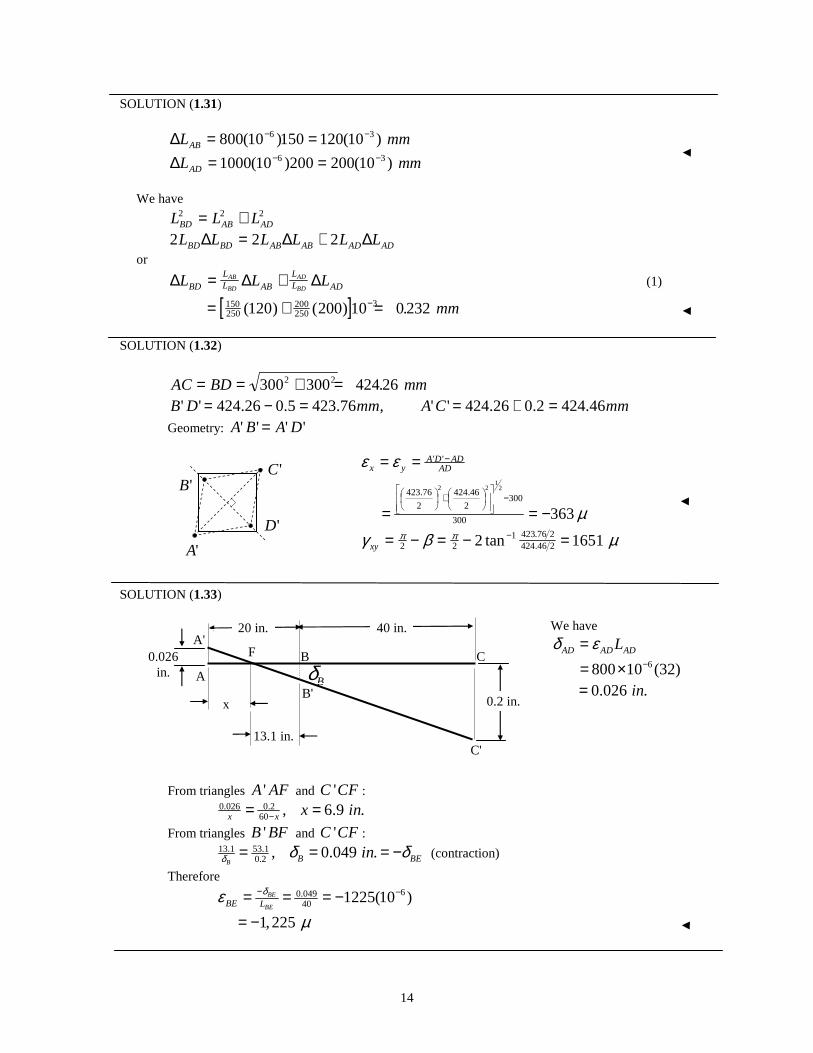
SOLUTION (1.33) We have

AD AD ADLδ ε=

6800 10 (32)−= ×

0.026 .in=

From triangles 'A AF and 'C CF :

0.026 0.260 , 6.9 .x x x in−= =

From triangles 'B BF and 'C CF :

13.1 53.10.2 , 0.049 .

B B BEinδ δ δ= = = − (contraction)

Therefore

60.04940 1225(10 )BE

BEBE Lδε − −= = = −

1,225µ= −

'B

'D

'C

'A

Bδ

F C

C'

x

A

0.026 in.

13.1 in.

B'

B A'

40 in. 20 in.

0.2 in.

15

SOLUTION (1.34)

( a ) ε µx = =0 00650 120. ε µy = = −−0 004

25 160.

γ µxy = − + = −1000 200 800

( b ) mmLL yABAB 996.24)00016.01(25)1(' =−=+= ε

mmLL xADAD 006.50)00012.01(50)1(' =+=+= ε

End of Chapter 1

16

CHAPTER 2 MATERIALS SOLUTION (2.1)

A in A inf0 42 3 2

42 3 205 196 35 10 05 0 00024 19616 10= = = − =− −π π( . ) . ( ) . , ( . . ) . ( ) .

We have ε µ ε µa t= = = =− −12 10

80 24 10

0 5

3 3

1500 480( ) . ( ).,

Thus

S ksipPA= = =−

0

3

3

4 10

196 35(1020 37( )

. ).

E psiS p

a

t

a= = = = =−ε

εεν20 37 10

1500 106

3

6 1358 10 0 32. ( )

( ). ( ) , .

Also

% ( ) .. ..reduction in area = =−196 35 196 16

196 35 100 0 097

SOLUTION (2.2) Normal stress is

2

500

(1 8)4

4744PA ksiπσ = = =

This is below the yield strength of 50 ksi (Table B.1). We have

0.318.5 12 0.001351 1351L

δε µ×= = = =

Hence

6

640,744

135(10 )30 10E psiσ

ε −= = = ×

SOLUTION (2.3)

The cross-sectional area: 20.5(0.25) 0.125 .o oA w t in= = =

( a ) Axial strain and axial stress are

0.003312.5 0.01324 1324aε µ= = =

4.80.125 38.4P

a A ksiσ = = =

Because a ySσ < (See Table B.1), Hooke's Law is valid.

( b ) Modulus of elasticity,

6

638,400

1324(10 )29 10a

aE psiσ

ε −= = = ×

( c ) Decrease in the width and thickness

0.3(0.5) 0.15 .ow w inν∆ = = =

0.3(0.24) 0.072 .ot t inν∆ = = =

15.0)100(% 8)10(12 3

==−

elongation

17

SOLUTION (2.4) Assume Hooke's Law applies. We have

1.55 300tε µ= − = −

3000.34 822t

aενε µ−= − = − =

Thus,

9 9(105 10 )(822 10 ) 92.61aE MPaσ ε −= = × × =

Since ySσ < , our assumption is valid.

So

2(92.61)( 4)(5) 1.818P A kNσ π= = =

SOLUTION (2.5) We obtain

L L mmAC BD= = + =15 15 21212 2 .

ε µxL

LAC

AC= = = −−∆ 2117 21 21

21 21 1886. ..

ε µyL

LBD

BD= = =−∆ 21 22 21 21

21 21 471. ..

( a ) E GPax

x= = =− −

σε

100

1886

6

6 53(10 )

(10 )

( b ) ν εε= = =y

x

4711886 0 25.

( c ) G GPa= =+53

2 0 25 212(1 . ) .

SOLUTION (2.6) Use generalized Hooke’s law:

ε ε ε σ σ σνx y z E x y z+ + = + +−1 2 ( ) (1)

For a constant triaxial state of stress: ε ε ε ε σ σ σ σx y z x y z= = = = = =,

Then, Eq. (1) becomes ε σν= −1 2E . Since σ and ε must have identical signs:

1 2 0− ≥ν or ν = 12

SOLUTION (2.7)

We have σ x ksi= =100 103 2

3

16 67( )( ) .

(CONT.)