MECE 4602 - Intro to Robotics

Project Group G

“Spine Needle Robot”

Professor Aleksandra Popovic

Spring 2012

Team: Xiaoming Lang, Brian Park, Jiali Wei, Hongda Zheng

1

Table of Contents

1. Analysis of Requirements ………………………………………………………….……………………….………… 2

a. Minimal Required Number of DOFs ………………………….…………………………………….… 2

b. Required Workspace ……………………………………………….……………………………………..… 2

c. Estimated Joint Speed ……………………………………….……………………………………………… 2

2. Proposal of Robot Kinematics ……………………….…………….…………………………………………….… 4

3. Kinematics of Robot ………………………………….…….…………………………………………………………… 7

a. Table of DH Parameters ……………………….…………………………………………………………… 7

b. Direct & Inverse Kinematics of Robot …….……………………………………………………….… 7

c. Workspace of Robot ……………………………….……………………………………………………. 10

4. Design of Robot …………………………….…………………….……………………………………………………. 11

a. Lengths & Thicknesses of Links ………………….…………………………………………………… 11

b. Materials for Links ……………………………………………………………………………………….…. 11

c. Computation of Dynamics Equations ……………………………………………………………… 12

d. Estimated Motor Requirements …………………………………………………………………….. 13

e. Types of Sensors Needed …………………………..………………………………………………….. 15

5. Appendix ……………………………………………………………………………………………………………………. 16

a. Matlab code …………………………………………………………………………………………………… 16

2

1. Analysis of Requirements

a. What is the minimal required number of DOFs to complete the task?

The minimum number of DOFs (Degrees of Freedom) is 3 for our spine needle robot. The

degrees of freedom we are dealing with are in the x-, y- and z-axis directions for the

movement of the robot and its links to successfully locate the point where the needle must

be inserted.

b. What is the required workspace?

A workspace here represents a three-dimensional volume of space in which a robot

performs its operations. In our particular case, the required workspace has the form of a

rectangular box that encompasses the spine region of a bigger-sized male (in order to

include all possible lengths and areas of a human spine). As a rough but safe estimate, we

have determined the region to be 100cm long, 25cm wide and 20cm deep.

c. What is the estimated speed of each joint?

We understand that it is quite difficult to figure out the exact values of speeds of each joint;

thus, we have to come up with reasonable estimates on how fast these joints must move.

We have looked particularly at the angular velocities and acceleration of the joints. They

should not be moving at such a high angular velocity and acceleration because doing so

would put too much torque on the joints, which would have a great chance to fail in a short

amount of time. On the other hand, the joints are not to move too slowly for the purpose of

increased time-saving and efficiency of the spine operations. Therefore, an acceptable

middle ground had to be chosen; the following table shows the values of angular velocities

and acceleration of each joint that we have determined:

Joint Angular Velocity (rad/s) Acceleration (rad/s2)

1 0.1 0.2

2 0.1 0.2

3 0.1 0.2

Table 1: Each joint’s angular velocities and acceleration of our choice

Having assumed the above values as our reasonable estimates of angular velocities and

accelerations of the joints, we have calculated the resulting torque that would be placed on

each joint. The results of the calculation is located in Section 4d.

3

The following figures show a few snapshots of the movement of our robot:

Figure 1: Snapshots of the spine needle robot movement

4

2. Proposal of Robot Kinematics

The simple kinematics of our robot is sketched below:

Figure 2: Overall kinematics of the spine needle robot

The most important element to consider when designing this robot was how to exactly find the

spot of a spine at which the needle must be inserted. It is extremely crucial to eliminate any

errors when the point of insertion is to be located because of the sheer gravity and severity of

the cases when the needle goes into the body with even a slight amount of offset, possibly

resulting in a paralysis or even death. Because the operation requires an utmost accuracy and

also since the spine of every patient is not guaranteed to be placed at the same location every

time, an imaging system such as X-ray or Ultrasound are commonly used to ensure that doctors

visually know exactly where the needle must be inserted.

Thus, we have concluded that, since locating the specific spot where the needle is to be inserted

is essential, we must ensure the accuracy with a combination of two methods: a rail on the side

of the operations table and a revolute joint attached to the rail. The rail can be either

automatically controlled by a computerized system or manually moved by a human hand or a

joystick. In either case, the rail must be programmed to have a coordinate system so, as the

robot attached to the rail moves, a computer can accurately track its movement along an axis

and display the current coordinates. That is, once the exact location of the needle insertion is

determined, a revolute joint on the rail is moved back and forth until the robot arm is

5

perpendicular to the point of insertion. If, for some reason, the revolute joint is slightly off from

where it must be or if there are multiple points of insertion, instead of always turning on the rail,

the revolute joint attached to the rail can just be rotated from being perpendicular to having a

certain amount of angle, θ0, in order to make small adjustments or refinements in finding the

exact location. A schematic of this is shown below in Figure 3.

After the robot is aligned with the insertion point, the links, L1 and L2, are used to place the

robot arm right over the insertion point. The angle between L1 and L2 needs to be either

enlarged or reduced to adjust to different distances at which the spine is located from the

revolute joint 0, and the way to do so is using the revolute joints 1 and 2. Based on small

discrepancies among the size and placement of each patient’s spine, the joints automatically

make the adjustments so that, ultimately, the revolute joint 3 will be located directly above the

spot for the needle to be inserted. Then, the needle, which is connected to a prismatic joint 4,

gets inserted vertically into the body and the spine and, after the operation is over, is taken out

perpendicularly again by controlling the movement of this prismatic joint. This is the basic

procedure that our robot follows to place its needle at a specific location on a patient’s body.

Figure 3: Top view of the spine needle robot setting

For our robot, the minimal required number of DOFs to complete an operation, as mentioned in

Part 1a, is 3. Joints 0 through 2 are the basic joints to meet this DOF requirement. However, our

proposed kinematics uses a total number of 5 DOFs, which are from four revolute joints and a

6

prismatic joint for the needle. There are a few factors to why the total number of degrees of

freedom increased from 3 to 5.

Some would think that, for the sole purpose of controlling the x, y and z coordinates of the

robot, the existence of the rail and Joints 3 and 4 are unnecessary and redundant. However,

these components are indispensible for our robot because of several reasons. First of all, the

presence of a rail can expand the workspace of our robot without requiring its arms to be too

long. With the rail, the robot arm would not need to become too horizontal, in which case the

torque would be much greater, in order to reach farther points. Also, the prismatic joint 4 is

necessary because the needle must be vertical. Without it, we cannot control both the position

and the orientation of the needle arbitrarily. The prismatic joint is also good for the robot

because, once it finds the (x, y) position for the needle to be inserted, the other joints can

remain stationary, increasing the stability of the robot (the needle will not change its orientation

due to the recalculation of the inverse kinematics). Therefore, we can control the inserting

process more precisely.

7

3. Kinematics of Robot

a. Write down a table of Denavit-Hartenberg (DH) parameters.

The following table summarizes the DH parameter results of our robot:

Link ai αi di φi

0 0 90° L0 φ1

1 L1 0 0 φ2

2 L2 0 0 φ3

3 L3 90° 0 φ4

Table 2: DH parameters of our robot

b. Compute direct and inverse kinematics of the robot.

Figure 4: x-y coordinates of Joints 1, 2 and 3

Direct Kinematics

As it can be seen from Figure 4, we have assigned each joint an x-y coordinate system. For

direct kinematics, we first find the transformation matrices between the links, which are

shown below:

8

0 0

0 0

01

0

cos 0 sin 0

sin 0 cos 0

0 1 0

0 0 0 1

TL

1 1 1 1

1 1 1 1

12

cos sin 0 cos

sin cos 0 sin

0 0 1 0

0 0 0 1

L

LT

2 2 2 2

2 2 2 2

23

cos sin 0 cos

sin cos 0 sin

0 0 1 0

0 0 0 1

L

LT

3 3 3 3

3 3 3 3

34

cos 0 sin cos

sin 0 cos cos

0 1 0 0

0 0 0 1

L

LT

Having found all of the transformation matrices, the complete matrix for the entire

transformation comes out to be:

1 2 3 0 0 1 2 3 0 0 1 1 2 1 2 3 1 2 3

1 2 3 0 0 1 2 31 2 3 0 0 0 1 1 2 1 2 3 1 2 3

04

1 2

cos( )cos sin sin( )cos cos ( cos cos( ) cos( ))

cos( ) cos( + + )cos( )sin cos sin ( cos cos( ) cos( ))

2 2

sin( +

L L L

L L LT

3 1 2 3 0 1 1 2 1 2 3 1 2 3) 0 cos( ) sin sin( ) sin( )

0 0 0 1

L L L L

Inverse Kinematics

It has been assumed that it is possible to find the exact coordinates of the needle

insertion point with respect to the origin set up on the operations table through various

methods. In other words, once Link 0 is fixed on the rail, we have information of the

exact coordinates of not only Link 0 but also where the needle has to be placed.

Figure 5: The spine needle robot system in the coordinate system view

9

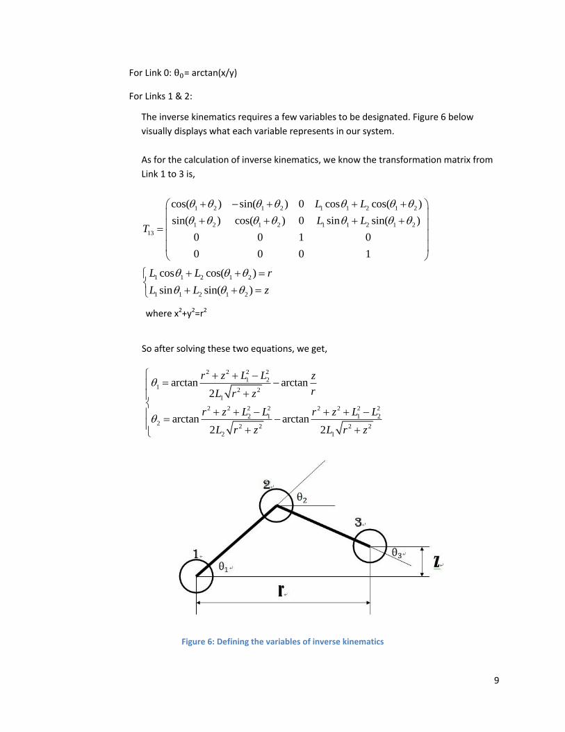
For Link 0: = arctan(x/y)

For Links 1 & 2:

The inverse kinematics requires a few variables to be designated. Figure 6 below

visually displays what each variable represents in our system.

As for the calculation of inverse kinematics, we know the transformation matrix from

Link 1 to 3 is,

1 2 1 2 1 1 2 1 2

1 2 1 2 1 1 2 1 2

13

cos( ) sin( ) 0 cos cos( )

sin( ) cos( ) 0 sin sin( )

0 0 1 0

0 0 0 1

L L

L LT

1 1 2 1 2

1 1 2 1 2

cos cos( )

sin sin( )

L L r

L L z

where x2+y2=r2

So after solving these two equations, we get,

2 2 2 2

1 21

2 2

1

2 2 2 2 2 2 2 2

2 1 1 22

2 2 2 2

2 1

arctan arctan2

arctan arctan2 2

r z L L z

rL r z

r z L L r z L L

L r z L r z

Figure 6: Defining the variables of inverse kinematics

10

For Link 3:

We need to put the needle at a vertical (perpendicular) orientation, so

. Thus,

For Link 4:

The function of Link 4 is to put the needle into the body; therefore, we do not need to

solve it in the positioning process.

c. What is the workspace of this robot? Does it have a dexterous workspace?

Our robot has two types of workspace combined into one. For the first type, when Joint 0

moves along the rail without rotating, the workspace of the robot would be a cylinder.

When the rail stops and Joint 0 is fixed on the rail, however, the robot would have a

spherical workspace in which the robot is allowed to rotate due to Joint 0. These two cases

may take place simultaneously for our robot.

Our robot has a dexterous workspace, it is part of the central line of link 0 being symmetric

to the center of link 1. The half length of this line is L1+L2-L3. The needle can reach points on

this line from every direction.

Figure 7: Workspace of the rpbot

11

4. Design of Robot

a. Propose lengths and thicknesses of all links.

We assume that the distance the robot should cover safely to reach the spine area is about

70cm, having determined proper dimensions of the operations table to be 2m long and 1m

wide. As a side note, the arc or the semicircular area of the robot arm is ignored in our

project due to the presence of a rail with which we can have a close-to-perfect alignment of

Joint 1 and the needle insertion point.

Next, we chose L1 = L2 = 45cm and this value ensures two things: 1) the robot arm can cover

all regions of the operations table, and 2) the angle between the two links is not too large

for the torque to be over an allowable limit, which can lead to a possible failure or fracture

of the links.

For Link 0, we choose L0 to be 25cm. Compared to the other values, this length does not

take on too much of an importance because we have the prismatic joint (Joint 4), which

enables us to adjust the vertical position of the needle, if necessary. But in order to not

make the link reasonable, we finally chose 25cm as its length.

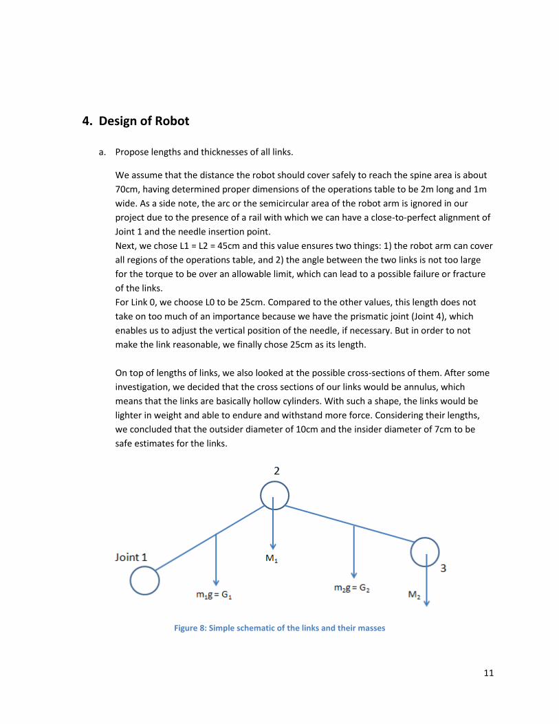
On top of lengths of links, we also looked at the possible cross-sections of them. After some

investigation, we decided that the cross sections of our links would be annulus, which

means that the links are basically hollow cylinders. With such a shape, the links would be

lighter in weight and able to endure and withstand more force. Considering their lengths,

we concluded that the outsider diameter of 10cm and the insider diameter of 7cm to be

safe estimates for the links.

Figure 8: Simple schematic of the links and their masses

12

b. Propose a material you want to use for the links.

We chose aluminum as the material of our robot. As mentioned above, the main goals of

the manufacturing of our robot is to build a light but strong product. Using aluminum would

result in a product that is not be too heavy to put much unnecessary pressure and force on

the operations table and the motors and also can provide a sufficient amount of strength to

avoid any fracture or breakdown.

c. Compute all dynamic equations (force propagation) for the robot.

Velocity Propagation:

1

1

0

0

,

2 21 1

2 1 2

0 0

0 0R

,

3 32 2

3 1 2 3

0 0

0 0R

So the velocity of each joint is:

1

0

0

0

v

,

2 1

2 21 1 1 12 1 1

0

( )

0

v R v t L

,

1 1 1

0 2

2 12 2 1 1 1

sin

cos

0

L

v R v L

1 1 2

3 2

3 32 2 2 23 2 1 2 2 1 1 2

sin

( ) cos

0

L

v R v t L L L

2 1 1 2 2 2 1 2 1 1 1

0 3

3 12 23 3 2 1 1 2 2 2 1 2 1 1 1

sin( ) sin( ) sin( )

cos( ) cos( ) cos( )

0

L L L

v R R v L L L

The velocities of Link 1 and 2 are,

13

1 1 1

0

2 1 1 1

sin

2

cos1

2 2

0

L

v Lvc

1 1 1 2

0 3

2 3 2 1 2 2 1 1 1 1 1 2

(sin sin )

2

cos cos2

2 2

0

L

v v L L L Lvc

With these velocities known, we could then obtain the kinetic energy and potential energy

using the following formulas:

Kinetic Energy:

0 0 0 0

1 2 2 2 3 3 1 2

1( ( ) ( ) ( 1) 1 ( 2) 2)

2

T T T TK m v v m v v g vc vc g vc vc

Potential Energy:

21 1 1 1 2 2 1 2 1 1 2 1 2 1 1

1( ) sin ( sin( ) sin ) ( sin( ) sin )2 2

LP G M L M L L G L

Since Lagrange Equation is known,

L K P

Torques for Motor 1 and 2 can be acquired using the following equations:

1

1 1

d L L

dx

,

2

2 2

d L L

dx

After we calculated and obtained all of the parameters, we then used Matlab to find the

values of the torque (a complete Matlab code can be found in the Appendix).

d. Estimate the requirements for motors. Find appropriate motors for this task.

14

Though our robot is a fairly small-sized one with only a handful of joints, the motors

attached to each joint would vary based on the torque required, weight of the links and

several other factors. Thus, according to their different situations and requirements, we

have researched and determined the most suitable motors for each of our robot’s joints.

Motor 0:

Motor 0 will not encounter too much torque and its weight is also not very important

because it is fixed on the rail. Thus, we selected 2642 012CXR.

Motors 1 & 2:

In order to specify which motors to use on Joints 1 and 2, we first look at their

parameters determined previously:

Link 1 Link 2

Length (m) 0.45 0.45

Outside Diameter (m) 0.10 0.10

Inside Diameter (m) 0.07 0.07

MaterialAluminum (density, ρ

= 2700 kg/m3)

Aluminum (density, ρ

= 2700 kg/m3)

Table 3: Parameters previously determined

Also, we calculated a few unknown parameters shown below:

Link 1 Link 2

Mass (kg) 1.549 1.549

Largest Angle (deg) 30 -60

Max Angular Velocity (rad/s) 0.1 0.1

Max Angular Acceleration (rad/s2) 0.2 0.2

Table 4: Calculated parameters

In addition to the calculated values above, another parameter needed to be determined:

torque of motors. However, since we had not specified which motors to use for each joint,

we decided to assume reasonable weight values for the motors such as 0.4 kg for Motor 2

and 0.3 kg for Motors 3 and 4. Having the knowledge of how heavy a typical motor to be

attached to a revolute or prismatic joint is, we chose a slightly higher value for Motor 2

because we believed that the possible torque that Joint 2 would experience is the greatest

out of all joints. Joint 2 connects L1 and L2 and, in case the angle between the two links

becomes large, there will be a great amount of torque applied to the joint. This is why we

have assigned a higher weight value to Motor 2, which will be attached to Joint 2.

15

With the assumed weights of motors, we can acquire the torques of Motors 1 & 2,

Torque1 = 21.22 Nm

Torque2 = 6.85 Nm

Since the moving speed of the robot is pretty slow, the stall torque and weight are the most

important factors in motor selection. We initially considered brushless DC motors; however,

we did not find any suitable ones that provide enough torque. So, we finally chose DC

motors from www.micromo.com.

Among more than 30 different DC motors on the website, we chose 3 candidates, whose

essential specifications are shown below, of our robot. The online links of these motors are

provided as well.

Motor Stall Torque (mNm) Weight (g)

3863 012C 1200 400

3272 012CR 1192 312

3257 048CR 547 242

Table 5: Specifications of motors considered for Joints 1 and 2

3863 012C: http://www.micromo.com/Micromo/DCMicroMotors/3863_C_DFF.pdf

3863 012CR: http://www.micromo.com/Micromo/DCMicroMotors/3272_cr_dff.pdf

3257 048CR: http://www.micromo.com/Micromo/DCMicroMotors/3257_CR_DFF.pdf

Actually, all of them have met the torque requirements with suitable gearhead. However,

3272 012CR motor has the largest torque/weight ratio, which is an important criterion for

our application. Therefore, after much consideration, we have chosen this particular motor

to be used for our robot.

Along with this motor, we chose 38A as the gearhead in order to increase the total torque.

For Motor 1, we use 3 gear stages and the reduction ratio of 36:1 while, for Motor 2, we use

2 gear stages and the reduction ratio of 12:1. Therefore, they can both provide enough stall

torque without exceeding the assumed weight above.

Motor 3:

The torque of Motor 3 can be smaller than others so 2657 012CR motor and 26A

gearhead will be sufficient.

Motor Stall Torque (mNm) Weight (g)

2657 012CR 278 156

Table 6: Specifications of the motor considered for Joint 3

16

2657 012CR: http://www.micromo.com/Micromo/DCMicroMotors/2657_CR_DFF.pdf

Motor 4:

Motor 4 is a linear motor and its peak force should be at least 10N to effectively insert

the needle into the spine according to the project requirements. It also must be quite

light in weight not to put too much force and weight on the joint to which the needle is

attached. A further research has shown us that LM 1247 060 01 motor meets the criteria

very well. The specifications and the online link of the motor is shown below:

Motor Peak Force (N) Weight (g)

LM 1247 060 01 10.7 67

Table 7: Specifications of the motor considered for Joint 4

LM 1247 060 01: http://www.micromo.com/Micromo/DCMicroMotors/2657_CR_DFF.pdf

e. What kind of sensors would you add to your robot? Where? Why?

The two most important factor we need to control are the position and the inserting force

and speed. The linear motor controller can tell us the inserting force and speed, so we do

not need some other sensors. And the X-ray device can be our sensor to some extend

because our need to get feedback from it to know what the precise position of the needle is

in real time to avoid dangerous circumstance cause by the control error or some other

reasons.

17

5. Appendix

a. Matlab code

function [ output_args ] = SpineNeedle( input_args )

syms th0 th1 th2 th3; syms d1 d2 d3; syms a1 a2 a3; syms L0 L1 L2 L3 D1 D2; syms m1 m2 g1 g2; syms M1 M2 G1 G2;

%Transformation Matrix T01=[cos(th0) 0 sin(th0) 0; sin(th0) 0 -cos(th0) 0; 0 1 0 L0; 0 0 0

1] T12=[cos(th1) -sin(th1) 0 L1*cos(th1); sin(th1) cos(th1) 0

L1*sin(th1); 0 0 1 0; 0 0 0 1] T23=[cos(th2) -sin(th2) 0 L2*cos(th2); sin(th2) cos(th2) 0

L2*sin(th2); 0 0 1 0; 0 0 0 1] T34=[cos(th3) 0 sin(th3) L3*cos(th3); sin(th3) 0 -cos(th3)

L3*sin(th3); 0 1 0 0; 0 0 0 1]

T21=inv(T12); T32=inv(T23);

R12=[cos(th1) -sin(th1) 0; sin(th1) cos(th1) 0; 0 0 1]; R23=[cos(th2) -sin(th2) 0; sin(th2) cos(th2) 0; 0 0 1]; t12=[L1*cos(th1);L1*sin(th1);0]; t23=[L2*cos(th2);L2*sin(th2);0];

R21=inv(R12); R32=inv(R23);

%Direct Kinematics: T13*[position in frame 3]=[position in frame 1] T13=(T12*T23) T04=simplify(T01*T12*T23*T34)

T31=(T32*T21); T13*[-L2/2;0;0;1]; T12*[0;0;0;1];

%Velocity Propagation w1=[0;0;d1]; w2=R21*w1+[0;0;d2]; w3=R32*w2+[0;0;d3];

v1=[0;0;0]; v2=simplify(R21*(v1+cross(w1,t12))) v3=(R32*(v2+cross(w2,t23))); %in their own frame

v2x=(R12*v2);

18

v3x=(R12*R23*v3); vc1=(1/2*v2x); vc2=simplify(1/2*(v2x+v3));

%Dynamics

K=1/2*(m1*transpose(v2x)*v2x+m2*transpose(v3x)*v3x+g1*transpose(vc1)

*vc1+g2*transpose(vc2)*vc2); P=(0.5*G1+M1)*L1*sin(th1)+M2*(L2*sin(th1 + th2) +

L1*sin(th1))+G2*( (L2*sin(th1 + th2))/2 + L1*sin(th1)); L=K-P;

%Motor 1 A=simplify(diff(L,d1)); B=simplify(diff(L,th1));

Torque1=(diff(A,d1)*a1+diff(A,d2)*a2+diff(A,th1)*d1+diff(A,th2)*d2)-

simplify(diff(L,th1));

%Motor 2 E=simplify(diff(L,d2)); F=simplify(diff(L,th2));

Torque2=(diff(E,d1)*a1+diff(E,d2)*a2+diff(E,th1)*d1+diff(E,th2)*d2)-

simplify(diff(L,th2));

L1=0.45; L2=0.45; D1=0.1; D2=0.07; p=2700; m1=(D1^2-D2^2)/4*p*L1; m2=(D1^2-D2^2)/4*p*L1; g1=0.4; g2=0.6; M1=m1*9.8; M2=m2*9.8; G1=g1*9.8; G2=g1*9.8;

th1=30/180*pi; th2=-60/180*pi; d1=0.1; d2=0.1; a1=0.2; a2=0.2;

subs(Torque1) subs(Torque2)

end