Measuring the Effects of a Land Value Tax on Land Development

Seong-Hoon Cho Agricultural Economics University of Tennessee

2621 Morgan Circle Knoxville TN 37996-4518

scho9utkedu

SeungGyu Kim Agricultural Economics University of Tennessee

2621 Morgan Circle Knoxville TN 37996-4518

sgkimutkedu

Roland K Roberts Agricultural Economics University of Tennessee

2621 Morgan Circle Knoxville TN 37996-4518

rrobert3utkedu

Selected Paper prepared for presentation at the Southern Agricultural Economics Association Annual Meeting Atlanta Georgia January 31-February 3 2009

Copyright 2009 by Cho et al All rights reserved Readers may make verbatim copies of this document for non-commercial purposes by any means provided that this copyright notice appears on all such copies

Measuring the Effects of a Land Value Tax on Land Development

Abstract The objective of this research is to evaluate a land value tax as a potential policy tool

to moderate sprawling development in Nashville TN the nationrsquos most sprawling metropolitan

community with a population of one million or moreTo achieve this objective the hypothesis is

empirically tested that a land value tax encourages more development closer to preexisting

development than farther from preexisting development Specifically the marginal effects of a

land value tax on the probability of land development is hypothesized to be greater in areas

around preexisting development than in areas more distant from preexisting development The

findings show that the marginal effects of a land value tax on the probability of developing

parcels that neighbored previously developed parcels was greater than the probability of

develping parcels that did not neighbor previously developed parcels This finding suggests that

land value taxation could be used to design compact development strategies that address

sprawling development

Keywords Land value tax Land development model Urban Sprawl

Measuring the Effects of a Land Value Tax on Land Development

Introduction

Urban sprawl has become a notable phenomenon in the United States since World War II

(Plantinga and Bernell 2005) Many urban areas are expanding while housing densities are

decreasing with urban areas growing at about twice the rate of the populations in many cities

(US Department of Housing and Urban Development 2000) Urban sprawl is well-described as

the leapfrogging of development beyond the cityrsquos outer boundary into smaller rural settlements

(Hanham and Spiker 2005) Rated as one of the most important local issues in 2000 (Princeton

Survey Research Associates 2000) urban sprawl has emerged as a challenging urban

development perplexity in the United States over the past few years A poll shows that 78 of

Americans support the control of urban sprawl in land use planning (Smart Growth America

2000)

Sprawl conditions appear to be worse in the South than elsewhere in the country

Recent population and economic growth in the South have contributed to pressures that create

sprawl Half of the top 10 most sprawling major US metro areas are in the South (Smart Growth

America 2003 Southeast Watershed Forum 2001) and half of the top 20 states that lost the

most open space and farmland to urban sprawl during the 1990rsquos are Southern States (Southeast

Watershed Forum 2001)

Nashville TN is an example of sprawl in the South It is identified as the nationrsquos most

sprawling metro area with a population of one million or more (Nasser and Overberg 2001) The

Nashville metro area had a population of approximately 12 million in 2000 with a projected

increase to two million within the next two decades (Cumberland Commercial Partners 2009

Alexander 2004) The US Census Bureau predicts that the population of Nashville will

1

outpacing most other major southern cities (Cumberland Commercial Partners 2009) A number

of service sectors eg schools and hospitals have been unable to keep pace with the rate of

growth

Of serious concern to planners is the rapidly increasing rate of land consumption

Between 1970 and 1990 Nashvillersquos population grew by 28 while its urbanized area grew by

41 (Sierra Club 2009) Land was reportedly developed at a rate of 60 acres per day during the

early 2000s (Chief Executive Magazine 2005) Much of this additional land consumption has

taken place in suburban or exurban areas causing loss of farmland and open space higher costs

of infrastructure and community services roadway congestion racial segregation and

concentrated poverty (Katz 2000 2002 Snyder and Bird 1998 Gordon and Richardson 1998

Daniels and Bowers 1997 Brookings 2000 Nelson and Sanchez 2005)

The negative effects of urban sprawl in Nashville have received increased scrutiny from

elected officials and other interested citizens attempting to moderate urban growth These

concerns have encouraged Nashvilles political leadership and its urban planners to tackle urban

sprawl through a strategic development initiative (Cumberland Commercial Partners 2009) The

main goal of the initiative is to moderate sprawl by directing future development closer to the

city center with more affordable urban housing and increased urban transit

The initiative has involved various instruments to moderate sprawl including zonal

territorial policies (eg zoning and growth boundary) and acquisition policies (eg conservation

easements purchase of and transfer of development rights government purchases of land for

parks and similar initiatives) Policy implementation in Nashville is particularly challenging

because many of the policy instruments are often viewed as an infringement on private property

2

rights that many Southerners hold as sacrosanct Thus there is interest in alternative instruments

other than zonal and acquisition types of policies to moderate sprawl in the area

A higher tax rate on land than on land improvement or a ldquoland value taxrdquo is a potential

policy tool to moderate sprawl in the Nashville area because it does not directly infringe on

private property rights The land value tax was first proposed by an American political economist

Henry George in the 19th Century as a way to eliminate land speculation In theory switching to

a higher land tax and a lower tax on structures can encourage compact development Because

land is immobile and higher land taxes reduce land prices land owners cannot avoid a tax on

land values or pass it on to land users Thus a higher land tax motivates landowners to generate

income to pay the tax The greatest economic incentive to develop land will exist where land

values are highest which is typically adjacent to preexisting development At the same time a

reduction in the tax rate applied to structures makes development of structures more profitable

On average areas far from preexisting development will have low land values and taxes and

thus less economic incentive for development (Rybeck 2004)

While appealing in theory only a handful of US municipalities including Pittsburgh

and a score of towns in Pennsylvania have implemented the land value tax There is limited

empirical evidence of the policy implications of implementing a two-rate property tax (different

rates for land and structures) for sprawl management (eg Bourassa 1990 Brueckner 1986

Brueckner and Kim 2003 Case and Grant 1991 Mills 1998 Nechyba 1998 Oates and Schwab

1997 Skaburskis 1995) The unpopularity of land value taxation in the United States flows from

two alleged legal obstacles ldquouniformity clausesrdquo which require that all taxation be applied

evenly within a jurisdiction and ldquoDillons Rulerdquo which implies that municipal corporations owe

their origins to and derive their powers and rights wholly from the legislature (Fisher 1997

3

Measuring the Effects of a Land Value Tax on Land Development

Abstract The objective of this research is to evaluate a land value tax as a potential policy tool

to moderate sprawling development in Nashville TN the nationrsquos most sprawling metropolitan

community with a population of one million or moreTo achieve this objective the hypothesis is

empirically tested that a land value tax encourages more development closer to preexisting

development than farther from preexisting development Specifically the marginal effects of a

land value tax on the probability of land development is hypothesized to be greater in areas

around preexisting development than in areas more distant from preexisting development The

findings show that the marginal effects of a land value tax on the probability of developing

parcels that neighbored previously developed parcels was greater than the probability of

develping parcels that did not neighbor previously developed parcels This finding suggests that

land value taxation could be used to design compact development strategies that address

sprawling development

Keywords Land value tax Land development model Urban Sprawl

Measuring the Effects of a Land Value Tax on Land Development

Introduction

Urban sprawl has become a notable phenomenon in the United States since World War II

(Plantinga and Bernell 2005) Many urban areas are expanding while housing densities are

decreasing with urban areas growing at about twice the rate of the populations in many cities

(US Department of Housing and Urban Development 2000) Urban sprawl is well-described as

the leapfrogging of development beyond the cityrsquos outer boundary into smaller rural settlements

(Hanham and Spiker 2005) Rated as one of the most important local issues in 2000 (Princeton

Survey Research Associates 2000) urban sprawl has emerged as a challenging urban

development perplexity in the United States over the past few years A poll shows that 78 of

Americans support the control of urban sprawl in land use planning (Smart Growth America

2000)

Sprawl conditions appear to be worse in the South than elsewhere in the country

Recent population and economic growth in the South have contributed to pressures that create

sprawl Half of the top 10 most sprawling major US metro areas are in the South (Smart Growth

America 2003 Southeast Watershed Forum 2001) and half of the top 20 states that lost the

most open space and farmland to urban sprawl during the 1990rsquos are Southern States (Southeast

Watershed Forum 2001)

Nashville TN is an example of sprawl in the South It is identified as the nationrsquos most

sprawling metro area with a population of one million or more (Nasser and Overberg 2001) The

Nashville metro area had a population of approximately 12 million in 2000 with a projected

increase to two million within the next two decades (Cumberland Commercial Partners 2009

Alexander 2004) The US Census Bureau predicts that the population of Nashville will

1

outpacing most other major southern cities (Cumberland Commercial Partners 2009) A number

of service sectors eg schools and hospitals have been unable to keep pace with the rate of

growth

Of serious concern to planners is the rapidly increasing rate of land consumption

Between 1970 and 1990 Nashvillersquos population grew by 28 while its urbanized area grew by

41 (Sierra Club 2009) Land was reportedly developed at a rate of 60 acres per day during the

early 2000s (Chief Executive Magazine 2005) Much of this additional land consumption has

taken place in suburban or exurban areas causing loss of farmland and open space higher costs

of infrastructure and community services roadway congestion racial segregation and

concentrated poverty (Katz 2000 2002 Snyder and Bird 1998 Gordon and Richardson 1998

Daniels and Bowers 1997 Brookings 2000 Nelson and Sanchez 2005)

The negative effects of urban sprawl in Nashville have received increased scrutiny from

elected officials and other interested citizens attempting to moderate urban growth These

concerns have encouraged Nashvilles political leadership and its urban planners to tackle urban

sprawl through a strategic development initiative (Cumberland Commercial Partners 2009) The

main goal of the initiative is to moderate sprawl by directing future development closer to the

city center with more affordable urban housing and increased urban transit

The initiative has involved various instruments to moderate sprawl including zonal

territorial policies (eg zoning and growth boundary) and acquisition policies (eg conservation

easements purchase of and transfer of development rights government purchases of land for

parks and similar initiatives) Policy implementation in Nashville is particularly challenging

because many of the policy instruments are often viewed as an infringement on private property

2

rights that many Southerners hold as sacrosanct Thus there is interest in alternative instruments

other than zonal and acquisition types of policies to moderate sprawl in the area

A higher tax rate on land than on land improvement or a ldquoland value taxrdquo is a potential

policy tool to moderate sprawl in the Nashville area because it does not directly infringe on

private property rights The land value tax was first proposed by an American political economist

Henry George in the 19th Century as a way to eliminate land speculation In theory switching to

a higher land tax and a lower tax on structures can encourage compact development Because

land is immobile and higher land taxes reduce land prices land owners cannot avoid a tax on

land values or pass it on to land users Thus a higher land tax motivates landowners to generate

income to pay the tax The greatest economic incentive to develop land will exist where land

values are highest which is typically adjacent to preexisting development At the same time a

reduction in the tax rate applied to structures makes development of structures more profitable

On average areas far from preexisting development will have low land values and taxes and

thus less economic incentive for development (Rybeck 2004)

While appealing in theory only a handful of US municipalities including Pittsburgh

and a score of towns in Pennsylvania have implemented the land value tax There is limited

empirical evidence of the policy implications of implementing a two-rate property tax (different

rates for land and structures) for sprawl management (eg Bourassa 1990 Brueckner 1986

Brueckner and Kim 2003 Case and Grant 1991 Mills 1998 Nechyba 1998 Oates and Schwab

1997 Skaburskis 1995) The unpopularity of land value taxation in the United States flows from

two alleged legal obstacles ldquouniformity clausesrdquo which require that all taxation be applied

evenly within a jurisdiction and ldquoDillons Rulerdquo which implies that municipal corporations owe

their origins to and derive their powers and rights wholly from the legislature (Fisher 1997

3

Measuring the Effects of a Land Value Tax on Land Development

Introduction

Urban sprawl has become a notable phenomenon in the United States since World War II

(Plantinga and Bernell 2005) Many urban areas are expanding while housing densities are

decreasing with urban areas growing at about twice the rate of the populations in many cities

(US Department of Housing and Urban Development 2000) Urban sprawl is well-described as

the leapfrogging of development beyond the cityrsquos outer boundary into smaller rural settlements

(Hanham and Spiker 2005) Rated as one of the most important local issues in 2000 (Princeton

Survey Research Associates 2000) urban sprawl has emerged as a challenging urban

development perplexity in the United States over the past few years A poll shows that 78 of

Americans support the control of urban sprawl in land use planning (Smart Growth America

2000)

Sprawl conditions appear to be worse in the South than elsewhere in the country

Recent population and economic growth in the South have contributed to pressures that create

sprawl Half of the top 10 most sprawling major US metro areas are in the South (Smart Growth

America 2003 Southeast Watershed Forum 2001) and half of the top 20 states that lost the

most open space and farmland to urban sprawl during the 1990rsquos are Southern States (Southeast

Watershed Forum 2001)

Nashville TN is an example of sprawl in the South It is identified as the nationrsquos most

sprawling metro area with a population of one million or more (Nasser and Overberg 2001) The

Nashville metro area had a population of approximately 12 million in 2000 with a projected

increase to two million within the next two decades (Cumberland Commercial Partners 2009

Alexander 2004) The US Census Bureau predicts that the population of Nashville will

1

outpacing most other major southern cities (Cumberland Commercial Partners 2009) A number

of service sectors eg schools and hospitals have been unable to keep pace with the rate of

growth

Of serious concern to planners is the rapidly increasing rate of land consumption

Between 1970 and 1990 Nashvillersquos population grew by 28 while its urbanized area grew by

41 (Sierra Club 2009) Land was reportedly developed at a rate of 60 acres per day during the

early 2000s (Chief Executive Magazine 2005) Much of this additional land consumption has

taken place in suburban or exurban areas causing loss of farmland and open space higher costs

of infrastructure and community services roadway congestion racial segregation and

concentrated poverty (Katz 2000 2002 Snyder and Bird 1998 Gordon and Richardson 1998

Daniels and Bowers 1997 Brookings 2000 Nelson and Sanchez 2005)

The negative effects of urban sprawl in Nashville have received increased scrutiny from

elected officials and other interested citizens attempting to moderate urban growth These

concerns have encouraged Nashvilles political leadership and its urban planners to tackle urban

sprawl through a strategic development initiative (Cumberland Commercial Partners 2009) The

main goal of the initiative is to moderate sprawl by directing future development closer to the

city center with more affordable urban housing and increased urban transit

The initiative has involved various instruments to moderate sprawl including zonal

territorial policies (eg zoning and growth boundary) and acquisition policies (eg conservation

easements purchase of and transfer of development rights government purchases of land for

parks and similar initiatives) Policy implementation in Nashville is particularly challenging

because many of the policy instruments are often viewed as an infringement on private property

2

rights that many Southerners hold as sacrosanct Thus there is interest in alternative instruments

other than zonal and acquisition types of policies to moderate sprawl in the area

A higher tax rate on land than on land improvement or a ldquoland value taxrdquo is a potential

policy tool to moderate sprawl in the Nashville area because it does not directly infringe on

private property rights The land value tax was first proposed by an American political economist

Henry George in the 19th Century as a way to eliminate land speculation In theory switching to

a higher land tax and a lower tax on structures can encourage compact development Because

land is immobile and higher land taxes reduce land prices land owners cannot avoid a tax on

land values or pass it on to land users Thus a higher land tax motivates landowners to generate

income to pay the tax The greatest economic incentive to develop land will exist where land

values are highest which is typically adjacent to preexisting development At the same time a

reduction in the tax rate applied to structures makes development of structures more profitable

On average areas far from preexisting development will have low land values and taxes and

thus less economic incentive for development (Rybeck 2004)

While appealing in theory only a handful of US municipalities including Pittsburgh

and a score of towns in Pennsylvania have implemented the land value tax There is limited

empirical evidence of the policy implications of implementing a two-rate property tax (different

rates for land and structures) for sprawl management (eg Bourassa 1990 Brueckner 1986

Brueckner and Kim 2003 Case and Grant 1991 Mills 1998 Nechyba 1998 Oates and Schwab

1997 Skaburskis 1995) The unpopularity of land value taxation in the United States flows from

two alleged legal obstacles ldquouniformity clausesrdquo which require that all taxation be applied

evenly within a jurisdiction and ldquoDillons Rulerdquo which implies that municipal corporations owe

their origins to and derive their powers and rights wholly from the legislature (Fisher 1997

3

outpacing most other major southern cities (Cumberland Commercial Partners 2009) A number

of service sectors eg schools and hospitals have been unable to keep pace with the rate of

growth

Of serious concern to planners is the rapidly increasing rate of land consumption

Between 1970 and 1990 Nashvillersquos population grew by 28 while its urbanized area grew by

41 (Sierra Club 2009) Land was reportedly developed at a rate of 60 acres per day during the

early 2000s (Chief Executive Magazine 2005) Much of this additional land consumption has

taken place in suburban or exurban areas causing loss of farmland and open space higher costs

of infrastructure and community services roadway congestion racial segregation and

concentrated poverty (Katz 2000 2002 Snyder and Bird 1998 Gordon and Richardson 1998

Daniels and Bowers 1997 Brookings 2000 Nelson and Sanchez 2005)

The negative effects of urban sprawl in Nashville have received increased scrutiny from

elected officials and other interested citizens attempting to moderate urban growth These

concerns have encouraged Nashvilles political leadership and its urban planners to tackle urban

sprawl through a strategic development initiative (Cumberland Commercial Partners 2009) The

main goal of the initiative is to moderate sprawl by directing future development closer to the

city center with more affordable urban housing and increased urban transit

The initiative has involved various instruments to moderate sprawl including zonal

territorial policies (eg zoning and growth boundary) and acquisition policies (eg conservation

easements purchase of and transfer of development rights government purchases of land for

parks and similar initiatives) Policy implementation in Nashville is particularly challenging

because many of the policy instruments are often viewed as an infringement on private property

2

rights that many Southerners hold as sacrosanct Thus there is interest in alternative instruments

other than zonal and acquisition types of policies to moderate sprawl in the area

A higher tax rate on land than on land improvement or a ldquoland value taxrdquo is a potential

policy tool to moderate sprawl in the Nashville area because it does not directly infringe on

private property rights The land value tax was first proposed by an American political economist

Henry George in the 19th Century as a way to eliminate land speculation In theory switching to

a higher land tax and a lower tax on structures can encourage compact development Because

land is immobile and higher land taxes reduce land prices land owners cannot avoid a tax on

land values or pass it on to land users Thus a higher land tax motivates landowners to generate

income to pay the tax The greatest economic incentive to develop land will exist where land

values are highest which is typically adjacent to preexisting development At the same time a

reduction in the tax rate applied to structures makes development of structures more profitable

On average areas far from preexisting development will have low land values and taxes and

thus less economic incentive for development (Rybeck 2004)

While appealing in theory only a handful of US municipalities including Pittsburgh

and a score of towns in Pennsylvania have implemented the land value tax There is limited

empirical evidence of the policy implications of implementing a two-rate property tax (different

rates for land and structures) for sprawl management (eg Bourassa 1990 Brueckner 1986

Brueckner and Kim 2003 Case and Grant 1991 Mills 1998 Nechyba 1998 Oates and Schwab

1997 Skaburskis 1995) The unpopularity of land value taxation in the United States flows from

two alleged legal obstacles ldquouniformity clausesrdquo which require that all taxation be applied

evenly within a jurisdiction and ldquoDillons Rulerdquo which implies that municipal corporations owe

their origins to and derive their powers and rights wholly from the legislature (Fisher 1997

3

rights that many Southerners hold as sacrosanct Thus there is interest in alternative instruments

other than zonal and acquisition types of policies to moderate sprawl in the area

A higher tax rate on land than on land improvement or a ldquoland value taxrdquo is a potential

policy tool to moderate sprawl in the Nashville area because it does not directly infringe on

private property rights The land value tax was first proposed by an American political economist

Henry George in the 19th Century as a way to eliminate land speculation In theory switching to

a higher land tax and a lower tax on structures can encourage compact development Because

land is immobile and higher land taxes reduce land prices land owners cannot avoid a tax on

land values or pass it on to land users Thus a higher land tax motivates landowners to generate

income to pay the tax The greatest economic incentive to develop land will exist where land

values are highest which is typically adjacent to preexisting development At the same time a

reduction in the tax rate applied to structures makes development of structures more profitable

On average areas far from preexisting development will have low land values and taxes and

thus less economic incentive for development (Rybeck 2004)

While appealing in theory only a handful of US municipalities including Pittsburgh

and a score of towns in Pennsylvania have implemented the land value tax There is limited

empirical evidence of the policy implications of implementing a two-rate property tax (different

rates for land and structures) for sprawl management (eg Bourassa 1990 Brueckner 1986

Brueckner and Kim 2003 Case and Grant 1991 Mills 1998 Nechyba 1998 Oates and Schwab

1997 Skaburskis 1995) The unpopularity of land value taxation in the United States flows from

two alleged legal obstacles ldquouniformity clausesrdquo which require that all taxation be applied

evenly within a jurisdiction and ldquoDillons Rulerdquo which implies that municipal corporations owe

their origins to and derive their powers and rights wholly from the legislature (Fisher 1997

3

Schoettle 2003) Notwithstanding the alleged legal obstacles the Supreme Court directly

acknowledged that a land value tax was constitutional so long as it was apportioned equally

among the states (Dixler 2006) Thus switching from the typical residential real estate property

tax in the United States in which the assessed values of land and structures are taxed equally to

a land value tax can be considered as an alternative sprawl management tool

The objective of this research is to evaluate the land value tax as a potential tool to

moderate sprawl development in the Nashville area To achieve this objective the hypothesis is

empirically tested that a land value tax encourages more development around preexisting

development than in areas distant from preexisting development Specifically the marginal

impact of a land value tax on the probabilities of land development is hypothesized to be greater

around preexisting development than the areas distant from preexisting development The

hypothesis is empirically tested using a land development model that corrects for spatial

dependence

Empirical Model

Land development decisions by a landowner at the parcel level have been modeled using discrete

choice models These models estimate the probability of land development as a function of

individual parcel-level attributes (eg Bockstael and Bell 1998 Bockstael 1996 Cho and

Newman 2005 Cho et al 2008 Bell and Irwin 2002 Irwin Bell and Geoghegan 2003 Irwin

and Bockstael 2002 2004)

We suppose that yt is a binary indicator of the choice whether to develop a parcel in time

period t (yt = 1) or not (yt = 0) Suppose the probability follows the logistic distribution then the

probability of land development is expressed as

4

(1) Prob (yt =1) = 1

t

t

ee

prime

prime+

β x

β x

where xt is a vector of exogenous variables explaining development decisions individual parcel

characteristics (ie distance and physical factors) neighborhood characteristics (ie

socioeconomic factors at the census-block group level) and tax on land value β is a vector of

parameter to be estimated

To control for spatial spillover effects of development from neighboring locations

equation (1) can be re-specified as

(2) Prob (yt =1) = 1

t t

t t

d

de

e

prime prime+α

prime prime+α+

β x

β x

where dt is a dummy variable indicating existence of development in the neighboring locations

around a parcel in time period t and α is a conformable parameter (dt = 1 if there is at least one

developed parcel in a parcelrsquos neighborhood in time period t 0 otherwise)

Because the existence of current development in the neighboring locations is expected to

be a function of the existence of past development in the neighboring locations it is

hypothesized that dt is a function of (dt-1 dt-2 hellip dt-p) where p is number of time lagged periods

Following a pth-order difference equation in a time series analysis dt can be generalized in the

following vector autoregression (VAR) form (Hamilton 1994 pp 291)

(3) 1 1 2 2 t t t p t pd d d dminus minus minus= φ + φ + + φ + w

whereφ is a conformable parameter and is an error term capturing random disturbances The

VAR model describes the existence of development in the neighboring locations over the current

period as a

w

linear function of the existence of past development in the neighboring locations

To the best of our knowledge there is no method in the land development literature that

suggests an adequate procedure for determining the order of the time lagged period p to capture

5

(1) Prob (yt =1) = 1

t

t

ee

prime

prime+

β x

β x

where xt is a vector of exogenous variables explaining development decisions individual parcel

characteristics (ie distance and physical factors) neighborhood characteristics (ie

socioeconomic factors at the census-block group level) and tax on land value β is a vector of

parameter to be estimated

To control for spatial spillover effects of development from neighboring locations

equation (1) can be re-specified as

(2) Prob (yt =1) = 1

t t

t t

d

de

e

prime prime+α

prime prime+α+

β x

β x

where dt is a dummy variable indicating existence of development in the neighboring locations

around a parcel in time period t and α is a conformable parameter (dt = 1 if there is at least one

developed parcel in a parcelrsquos neighborhood in time period t 0 otherwise)

Because the existence of current development in the neighboring locations is expected to

be a function of the existence of past development in the neighboring locations it is

hypothesized that dt is a function of (dt-1 dt-2 hellip dt-p) where p is number of time lagged periods

Following a pth-order difference equation in a time series analysis dt can be generalized in the

following vector autoregression (VAR) form (Hamilton 1994 pp 291)

(3) 1 1 2 2 t t t p t pd d d dminus minus minus= φ + φ + + φ + w

whereφ is a conformable parameter and is an error term capturing random disturbances The

VAR model describes the existence of development in the neighboring locations over the current

period as a

w

linear function of the existence of past development in the neighboring locations

To the best of our knowledge there is no method in the land development literature that

suggests an adequate procedure for determining the order of the time lagged period p to capture

5

the existence of current development in neighboring locations On the other hand order selection

based on the Akaike Information Criterion (AIC) (Akaike 1974 Schwarz 1978 Hannan and

Quinn 1979) are often applied in time series model selection AIC is chosen as an order selection

criterion in this study because the error of asymptotic normality is small and the degree of

accuracy of the AIC is high for large and realistic sample sizes (Shao 1997 Shinkai et al 2008)

A series of VAR models (3) for p = 1 2 hellip n generates AICs for different orders of time

lagged periods Once the p that minimizes AIC is identified equation (2) can be re-specified by

substituting dt into equation (3)

(4) Prob (yt =1) = 1 1 2 2

1 1 2 2

1

t t t p t p

t t t p t p

d d d w

d d d we

e

minus minus minus

minus minus minus

prime +φ +φ + +φ +

prime +φ +φ + +φ ++

β x

β x

Equation (4) can be estimated for the full sample and a separate regression for each of the sample

regimes determined by the existence of past development in the neighboring locations (dt-1 dt-2

hellip dt-p) For example if the optimal time lag is identified as p = 2 sample regimes are divided

into four (dt-1 = 1 and dt-2 = 1 dt-1 = 1 and dt-2 = 0 dt-1 = 0 and dt-2 = 1 and dt-1 = 0 and dt-2 = 0)

A likelihood ratio (LR) test is used to verify whether the model should be estimated with

separate regressions for the four sample regimes or a single pooled regression Denoting the

maximum log-likelihoods for the four sample regimes and pooled regressions (with time-lagged

dummy variables in the equation) as f[1] f[2] f[3] f[4] and fP with corresponding numbers of

parameters k[1] k[2] k[3] k[4] and kP then the LR statistic 2(f[1] + f[2] + f[3] + f[4] minus fP) is Chi-

square distributed with (k[1] + k[2] + k[3] + k[4] minus kP) degrees of freedom

The model can be used to evaluate the effects of alternative variables on land

development For example the marginal effect of a land value tax on the probability of land

development equals 1 1 2 2Pr [ 1] ( )tt t t t t p t pob y f d d d wminus minus minus τprimepart = partτ = + φ + φ + + φ +β x β where

tτβ is

the coefficient on the land value tax and f is the logistic density function given by

6

1 1 2 2 1 1 2 2( ) ( )[1 ( )]t t t t p t p t t t p t pd d d w d d d wminus minus minus minus minus minusprime prime primeγ = Λ + φ + φ + + φ + minusΛ + φ + φ + + φ +β x β x β x

where Λ is logistic distribution

The parameters in equation (4) are estimated by the generalized method of moments

(GMM) estimator to address potential interactions in land development (Conley 1999 Conley

and Udry 2005) Heteroskedasticity consistent standard errors are estimated to remove residual

spatial autocorrelation caused by codetermined development decisions The covariance-matrix

estimators are modified to allow regression disturbance terms to be correlated across

neighborhood parcels as a general function of their Euclidean distances The error term is

permitted to be conditionally heteroskedastic and spatially correlated across parcels using the

spatial GMM approach

Study Area and Data

Four major GIS data sets are used to collect data for Nashville-Davison County Tennessee

individual parcel data census-block group data boundary data and environmental feature data

The individual parcel data are obtained from the Metro Planning Department Davidson County

(MPD 2008) and the Davidson County Tax Assessors Office The study area consists of 467

census-block groups Information from these census-block groups such as per capita income and

unemployment rate is assigned to parcels located within the boundaries of the census-block

groups Boundary data ie high school districts and jurisdiction boundaries are obtained from

MPD Environmental feature data ie water bodies and golf courses are collected from

Environmental Systems Research Institute Data and Maps 2004 (ESRI 2004) Other

environmental feature data ie shape files for railroads and parks are acquired from MPD

7

Definitions of variables used in the regressions are listed in Table 1 and detailed statistics for the

variables are reported in Table 2

Dummy variables indicating the existence of development in the neighboring locations

around parcel i in time period t t-1hellip and t-p (dt dt-1hellip and dt-p) are created based on a

minimum threshold spatial matrix using GeoDarsquos (GeoDa Center 2009) default distance

threshold (Anselin 2004) The default distance threshold ensures that every observation has at

least one neighbor observation When observations are coupled with their closest observations

the minimum threshold is the distance between the pair whose distance is the longest among the

pairs The minimum threshold spatial matrix enables the creation of a dummy variable that takes

on a value of 1 if any development exists in a time period within the minimum threshold and 0

otherwise The default distance in our data is identified as 3657 feet (about 09 mile) The

correlation decreases as the time lag increases For example the correlations of 2007 dummy

variable with dummy variables for 2006 2000 1997 and 1994 are 054 036 021 and 017

respectively

At the start of 2007 the number of vacant arcels in Nashville-Davison County was

22244 Developed parcels are defined as single-family houses that were built during 2007 Only

single-family housing development is considered in the model because the development decision

process for different land uses are influence by different development factors and property

characteristics After eliminating parcels developed to other land uses 19606 useable

observations remained Of the 19606 parcels 1718 parcels (88 ) were developed for single-

family housing during 2007 The average size of undeveloped parcels was 162885 square feet

(37 acres) whereas the average size of parcels developed for single-family housing was 17102

8

square feet (04 acres) Smaller sizes of developed parcels indicate that parcels are segmented

when they are developed for a single-family housing

Empirical Results

Figure 1 shows the percentage change in AIC with respect to an increase in the time lag period p

where time period t is 2007 A significant drop of AIC (8) is observed from

to Beyond the 2005 lagged period the percentage change in AIC

remains relatively small (within 2) indicating insignificant gain of goodness-of-fit with

additional time lagged variables in the model Thus equation (4) could be estimated for the full

sample with d

2007 1 2006d d= φ +w

w2007 1 2006 2 2005d d d= φ + φ +

2006 and d2005 in the model and a separate regression for each of the four sample

regimes ie [1] d2006 = 1 and d2005 = 1 [2] d2006 = 1 and d2005 = 0 [3] d2006 = 0 and d2005 = 1 and

[4] d2006 = 0 and d2005 = 0 Parcels in sample regimes [1] and [2] were the most developed (11

and 6 of the parcels developed respectively) See Figure 2 for spatial distributions of the

sample regimes

The null hypothesis that all slope parameters (ie except the constants) are equal is

rejected (LR =23044 df = 54 p-value lt 0001) suggesting that the inclusion of time-lagged

dummy variables in the pooled regression does not fully capture spatial differences in the

existence of preexisting development in neighboring locations and thus separate regressions for

the four sample regimes are appropriate

Marginal effects based on parameter estimates for each sample regime using the spatial

GMM approach are presented in Table 3 The effects of proximity to water body proximity to

golf course proximity to central business districts (CBD) proximity to greenway proximity to

railroad proximity to interstate highway and slope variables are found to be significant at the

9

5 level in at least one of the four sample regimes The discussion below is limited to variables

that are statistically significant at the 5 level

Parcels farther from water bodies were more likely to be developed for single-family

housing for sample regime [2] The negative effects of proximity to water bodies may be

explained by the fact that undeveloped land closer to water bodies was already developed prior

to 2007 The parcels closer to a golf course were more likely to be developed for sample regimes

[2] and [4] reflecting the recent development of golf courses within residential communities in

suburban area (eg River Landing Subdivision near Riverside Golf Course and Pennington

Bend Chase Subdivision near Springhouse Golf Course) Parcels farther from the CBD were

more likely to be developed for spatial regime [1] The negative effects of proximity to the CBD

reflect a scarcity of developable parcels closer to the CBD An increase in distance to a railroad

increases the probability of development for sample regimes [1] and [2] The negative effect of

proximity to a railroad is likely due to noise disamenities or inconvenience A decrease in

distance to an interstate highway increases the probability of development for sample regime [3]

and decreases the probability of development for sample regime [4] The negative effect is likely

due to noise disamenities associated with interstate highway traffic whereas the positive effect is

likely due to the convenience of being closer to the interstate highway A decrease in slope (ie

flatter building surfaces) increases the probability of development for sample regimes [1] [2]

and [4] whereas the opposite is the case for sample regime [3]

The probability of development increases as the tax rate on land value per acre increases

in all four sample regimes (with current tax rate of $269 per $100 of assessed value in the

county per year) An increase in the tax rate on land value per acre by $1000 (or tax rate of

$384 per $100 of assessed value per year) increases the probability of development by 25 4

10

5 and 1 for sample regimes [1] [2] [3] and [4] respectively These results reveal a

substantially greater marginal effect for sample regime [1] than for the other sample regimes

with the lowest marginal effect for sample regime [4] This finding implies that marginal effect

of a land value tax on the probability of land development in 2007 is greater for parcels with

neighboring development in 2006 and 2005 than for parcels that did not have developed

neighboring parcels in 2006 and 2005 Thus the marginal effect of a land value tax on the

probability of land development is greater around preexisting development than in areas distant

from preexisting development This finding empirically validates the hypothesis that a land value

tax encourages more development around preexisting development than in areas where

preexisting development does not exist

Conclusions

Compact development is a key component in reducing the pressure of urban sprawl Compact

development can be achieved by encouraging the development of vacant land parcels in

neighborhoods where development already exists Our objective was to determine if a land value

tax would be an effective policy tool in promoting compact development in Nashville TN A

land development model was used to evaluate the hypothesis that a land value tax increases the

probability of land development in neighborhoods where development already exists relative to

areas distant from preexisting development Results show that the marginal effect of a land value

tax on the probability of a vacant lot being developed in 2007 is greater for parcels in

neighborhoods with preexisting development in 2006 and 2005 than for parcels in neighborhoods

without preexisting development in those years This finding suggests that land value taxation

could be used to design compact development strategies to address sprawl in the Nashville area

11

This research benefits local community leaders involved with land-use policy decision

making and property tax law in the Nashville area The quantitative estimates produced by this

research are uniquely suited to those policy makers as they consider land value taxation as a

policy tool to moderate sprawl development Further the methods and procedures presented in

this research could be used by policy makers in other metro areas where similar data are

available

The heterogeneous effects of a land value tax across the sample regimes specified in this

research can help decision makers establish land use development patterns that make the most

efficient and feasible use of existing infrastructure and public services The results also provide

guidelines for new development that maintains or enhances the quality of the Nashville area For

example policy makers could make more efficient use of existing infrastructure and public

services in previously developed parts of the Nashville area through land value taxation that

encourages growth toward locations where development infrastructure and public services

already exist

12

References

Akaike H 1974 ldquoA new look at the statistical model identificationrdquo IEEE Transactions on Automatic Control AC-19 716-723

Alexander M 2004 The ldquoCreative Classrdquo and Economic Development An Analysis of

Workforce Attraction and Retention in the Atlanta Region (httpwwwcherrygatechedurefsstudentAlexanderFinalPaper2004pdf)

Anselin L and DA Griffith 1988 ldquoDo spatial effects really matter in regression analysisrdquo

Papers of Regional Science Association 65 11-34 Bell K EG Irwin 2002 ldquoSpatially-explicit micro-level modeling of land use change at the

rural-urban interfacerdquo Agricultural Economics 27 217-232 Bockstael N 1996 ldquoModeling economics and ecology the importance of a spatial perspectiverdquo

American Journal of Agricultural Economics 78 1168-1180 Bockstael N K Bell 1998 Land use patterns and water quality the effect of differential land

management controls In Just R S Netanyahu (Eds) International Water and Resource Economics Consortium Conflict and Cooperation on Trans-Boundary Water Resources Kluwater Academic Publishers Dordrecht

Bourassa SC 1990 ldquoLand value taxation and housing development effects of property tax

three types of citiesrdquo American Journal of Economics and Sociology 49 101-111 Brookings Institute 2000 ldquoMoving beyond sprawl the challenge for metropolitan Atlantardquo

Center on Urban and Metropolitan Policy (httpwwwbrookingseduurban) Brueckner J K 1986 ldquoA modern analysis of the effects of site value taxationrdquo National Tax

Journal 39 49-58 Brueckner J and H Kim 2003 ldquoUrban sprawl and the property taxrdquo International Tax and

Public Finance 10 (1) 5-23 Case K E and J H Grant 1991 ldquoProperty tax incidence in a multijurisdictional neoclassical

modelrdquo Public Finance Quarterly 19 (4) 379-92 Chief Executive Magazine 2005 Southern Sprawl

(httpwwwchiefexecutivenetME2Audiencesdirmodaspsid=ampnm=amptype=Publishingampmod=Publications3A3AArticleampmid=8F3A7027421841978F18BE895F87F791amptier=4ampid=25FE1538F987419E98A5D1094B2DCC87ampAudID=50244528DF294421884F1F64425AAA1E)

Cho S and D H Newman 2005 ldquoSpatial analysis of rural land developmentrdquo Forest Policy

and Economics 7 732-744

13

1 1 2 2 1 1 2 2( ) ( )[1 ( )]t t t t p t p t t t p t pd d d w d d d wminus minus minus minus minus minusprime prime primeγ = Λ + φ + φ + + φ + minusΛ + φ + φ + + φ +β x β x β x

where Λ is logistic distribution

The parameters in equation (4) are estimated by the generalized method of moments

(GMM) estimator to address potential interactions in land development (Conley 1999 Conley

and Udry 2005) Heteroskedasticity consistent standard errors are estimated to remove residual

spatial autocorrelation caused by codetermined development decisions The covariance-matrix

estimators are modified to allow regression disturbance terms to be correlated across

neighborhood parcels as a general function of their Euclidean distances The error term is

permitted to be conditionally heteroskedastic and spatially correlated across parcels using the

spatial GMM approach

Study Area and Data

Four major GIS data sets are used to collect data for Nashville-Davison County Tennessee

individual parcel data census-block group data boundary data and environmental feature data

The individual parcel data are obtained from the Metro Planning Department Davidson County

(MPD 2008) and the Davidson County Tax Assessors Office The study area consists of 467

census-block groups Information from these census-block groups such as per capita income and

unemployment rate is assigned to parcels located within the boundaries of the census-block

groups Boundary data ie high school districts and jurisdiction boundaries are obtained from

MPD Environmental feature data ie water bodies and golf courses are collected from

Environmental Systems Research Institute Data and Maps 2004 (ESRI 2004) Other

environmental feature data ie shape files for railroads and parks are acquired from MPD

7

Definitions of variables used in the regressions are listed in Table 1 and detailed statistics for the

variables are reported in Table 2

Dummy variables indicating the existence of development in the neighboring locations

around parcel i in time period t t-1hellip and t-p (dt dt-1hellip and dt-p) are created based on a

minimum threshold spatial matrix using GeoDarsquos (GeoDa Center 2009) default distance

threshold (Anselin 2004) The default distance threshold ensures that every observation has at

least one neighbor observation When observations are coupled with their closest observations

the minimum threshold is the distance between the pair whose distance is the longest among the

pairs The minimum threshold spatial matrix enables the creation of a dummy variable that takes

on a value of 1 if any development exists in a time period within the minimum threshold and 0

otherwise The default distance in our data is identified as 3657 feet (about 09 mile) The

correlation decreases as the time lag increases For example the correlations of 2007 dummy

variable with dummy variables for 2006 2000 1997 and 1994 are 054 036 021 and 017

respectively

At the start of 2007 the number of vacant arcels in Nashville-Davison County was

22244 Developed parcels are defined as single-family houses that were built during 2007 Only

single-family housing development is considered in the model because the development decision

process for different land uses are influence by different development factors and property

characteristics After eliminating parcels developed to other land uses 19606 useable

observations remained Of the 19606 parcels 1718 parcels (88 ) were developed for single-

family housing during 2007 The average size of undeveloped parcels was 162885 square feet

(37 acres) whereas the average size of parcels developed for single-family housing was 17102

8

square feet (04 acres) Smaller sizes of developed parcels indicate that parcels are segmented

when they are developed for a single-family housing

Empirical Results

Figure 1 shows the percentage change in AIC with respect to an increase in the time lag period p

where time period t is 2007 A significant drop of AIC (8) is observed from

to Beyond the 2005 lagged period the percentage change in AIC

remains relatively small (within 2) indicating insignificant gain of goodness-of-fit with

additional time lagged variables in the model Thus equation (4) could be estimated for the full

sample with d

2007 1 2006d d= φ +w

w2007 1 2006 2 2005d d d= φ + φ +

2006 and d2005 in the model and a separate regression for each of the four sample

regimes ie [1] d2006 = 1 and d2005 = 1 [2] d2006 = 1 and d2005 = 0 [3] d2006 = 0 and d2005 = 1 and

[4] d2006 = 0 and d2005 = 0 Parcels in sample regimes [1] and [2] were the most developed (11

and 6 of the parcels developed respectively) See Figure 2 for spatial distributions of the

sample regimes

The null hypothesis that all slope parameters (ie except the constants) are equal is

rejected (LR =23044 df = 54 p-value lt 0001) suggesting that the inclusion of time-lagged

dummy variables in the pooled regression does not fully capture spatial differences in the

existence of preexisting development in neighboring locations and thus separate regressions for

the four sample regimes are appropriate

Marginal effects based on parameter estimates for each sample regime using the spatial

GMM approach are presented in Table 3 The effects of proximity to water body proximity to

golf course proximity to central business districts (CBD) proximity to greenway proximity to

railroad proximity to interstate highway and slope variables are found to be significant at the

9

5 level in at least one of the four sample regimes The discussion below is limited to variables

that are statistically significant at the 5 level

Parcels farther from water bodies were more likely to be developed for single-family

housing for sample regime [2] The negative effects of proximity to water bodies may be

explained by the fact that undeveloped land closer to water bodies was already developed prior

to 2007 The parcels closer to a golf course were more likely to be developed for sample regimes

[2] and [4] reflecting the recent development of golf courses within residential communities in

suburban area (eg River Landing Subdivision near Riverside Golf Course and Pennington

Bend Chase Subdivision near Springhouse Golf Course) Parcels farther from the CBD were

more likely to be developed for spatial regime [1] The negative effects of proximity to the CBD

reflect a scarcity of developable parcels closer to the CBD An increase in distance to a railroad

increases the probability of development for sample regimes [1] and [2] The negative effect of

proximity to a railroad is likely due to noise disamenities or inconvenience A decrease in

distance to an interstate highway increases the probability of development for sample regime [3]

and decreases the probability of development for sample regime [4] The negative effect is likely

due to noise disamenities associated with interstate highway traffic whereas the positive effect is

likely due to the convenience of being closer to the interstate highway A decrease in slope (ie

flatter building surfaces) increases the probability of development for sample regimes [1] [2]

and [4] whereas the opposite is the case for sample regime [3]

The probability of development increases as the tax rate on land value per acre increases

in all four sample regimes (with current tax rate of $269 per $100 of assessed value in the

county per year) An increase in the tax rate on land value per acre by $1000 (or tax rate of

$384 per $100 of assessed value per year) increases the probability of development by 25 4

10

5 and 1 for sample regimes [1] [2] [3] and [4] respectively These results reveal a

substantially greater marginal effect for sample regime [1] than for the other sample regimes

with the lowest marginal effect for sample regime [4] This finding implies that marginal effect

of a land value tax on the probability of land development in 2007 is greater for parcels with

neighboring development in 2006 and 2005 than for parcels that did not have developed

neighboring parcels in 2006 and 2005 Thus the marginal effect of a land value tax on the

probability of land development is greater around preexisting development than in areas distant

from preexisting development This finding empirically validates the hypothesis that a land value

tax encourages more development around preexisting development than in areas where

preexisting development does not exist

Conclusions

Compact development is a key component in reducing the pressure of urban sprawl Compact

development can be achieved by encouraging the development of vacant land parcels in

neighborhoods where development already exists Our objective was to determine if a land value

tax would be an effective policy tool in promoting compact development in Nashville TN A

land development model was used to evaluate the hypothesis that a land value tax increases the

probability of land development in neighborhoods where development already exists relative to

areas distant from preexisting development Results show that the marginal effect of a land value

tax on the probability of a vacant lot being developed in 2007 is greater for parcels in

neighborhoods with preexisting development in 2006 and 2005 than for parcels in neighborhoods

without preexisting development in those years This finding suggests that land value taxation

could be used to design compact development strategies to address sprawl in the Nashville area

11

This research benefits local community leaders involved with land-use policy decision

making and property tax law in the Nashville area The quantitative estimates produced by this

research are uniquely suited to those policy makers as they consider land value taxation as a

policy tool to moderate sprawl development Further the methods and procedures presented in

this research could be used by policy makers in other metro areas where similar data are

available

The heterogeneous effects of a land value tax across the sample regimes specified in this

research can help decision makers establish land use development patterns that make the most

efficient and feasible use of existing infrastructure and public services The results also provide

guidelines for new development that maintains or enhances the quality of the Nashville area For

example policy makers could make more efficient use of existing infrastructure and public

services in previously developed parts of the Nashville area through land value taxation that

encourages growth toward locations where development infrastructure and public services

already exist

12

References

Akaike H 1974 ldquoA new look at the statistical model identificationrdquo IEEE Transactions on Automatic Control AC-19 716-723

Alexander M 2004 The ldquoCreative Classrdquo and Economic Development An Analysis of

Workforce Attraction and Retention in the Atlanta Region (httpwwwcherrygatechedurefsstudentAlexanderFinalPaper2004pdf)

Anselin L and DA Griffith 1988 ldquoDo spatial effects really matter in regression analysisrdquo

Papers of Regional Science Association 65 11-34 Bell K EG Irwin 2002 ldquoSpatially-explicit micro-level modeling of land use change at the

rural-urban interfacerdquo Agricultural Economics 27 217-232 Bockstael N 1996 ldquoModeling economics and ecology the importance of a spatial perspectiverdquo

American Journal of Agricultural Economics 78 1168-1180 Bockstael N K Bell 1998 Land use patterns and water quality the effect of differential land

management controls In Just R S Netanyahu (Eds) International Water and Resource Economics Consortium Conflict and Cooperation on Trans-Boundary Water Resources Kluwater Academic Publishers Dordrecht

Bourassa SC 1990 ldquoLand value taxation and housing development effects of property tax

three types of citiesrdquo American Journal of Economics and Sociology 49 101-111 Brookings Institute 2000 ldquoMoving beyond sprawl the challenge for metropolitan Atlantardquo

Center on Urban and Metropolitan Policy (httpwwwbrookingseduurban) Brueckner J K 1986 ldquoA modern analysis of the effects of site value taxationrdquo National Tax

Journal 39 49-58 Brueckner J and H Kim 2003 ldquoUrban sprawl and the property taxrdquo International Tax and

Public Finance 10 (1) 5-23 Case K E and J H Grant 1991 ldquoProperty tax incidence in a multijurisdictional neoclassical

modelrdquo Public Finance Quarterly 19 (4) 379-92 Chief Executive Magazine 2005 Southern Sprawl

(httpwwwchiefexecutivenetME2Audiencesdirmodaspsid=ampnm=amptype=Publishingampmod=Publications3A3AArticleampmid=8F3A7027421841978F18BE895F87F791amptier=4ampid=25FE1538F987419E98A5D1094B2DCC87ampAudID=50244528DF294421884F1F64425AAA1E)

Cho S and D H Newman 2005 ldquoSpatial analysis of rural land developmentrdquo Forest Policy

and Economics 7 732-744

13

Definitions of variables used in the regressions are listed in Table 1 and detailed statistics for the

variables are reported in Table 2

Dummy variables indicating the existence of development in the neighboring locations

around parcel i in time period t t-1hellip and t-p (dt dt-1hellip and dt-p) are created based on a

minimum threshold spatial matrix using GeoDarsquos (GeoDa Center 2009) default distance

threshold (Anselin 2004) The default distance threshold ensures that every observation has at

least one neighbor observation When observations are coupled with their closest observations

the minimum threshold is the distance between the pair whose distance is the longest among the

pairs The minimum threshold spatial matrix enables the creation of a dummy variable that takes

on a value of 1 if any development exists in a time period within the minimum threshold and 0

otherwise The default distance in our data is identified as 3657 feet (about 09 mile) The

correlation decreases as the time lag increases For example the correlations of 2007 dummy

variable with dummy variables for 2006 2000 1997 and 1994 are 054 036 021 and 017

respectively

At the start of 2007 the number of vacant arcels in Nashville-Davison County was

22244 Developed parcels are defined as single-family houses that were built during 2007 Only

single-family housing development is considered in the model because the development decision

process for different land uses are influence by different development factors and property

characteristics After eliminating parcels developed to other land uses 19606 useable

observations remained Of the 19606 parcels 1718 parcels (88 ) were developed for single-

family housing during 2007 The average size of undeveloped parcels was 162885 square feet

(37 acres) whereas the average size of parcels developed for single-family housing was 17102

8

square feet (04 acres) Smaller sizes of developed parcels indicate that parcels are segmented

when they are developed for a single-family housing

Empirical Results

Figure 1 shows the percentage change in AIC with respect to an increase in the time lag period p

where time period t is 2007 A significant drop of AIC (8) is observed from

to Beyond the 2005 lagged period the percentage change in AIC

remains relatively small (within 2) indicating insignificant gain of goodness-of-fit with

additional time lagged variables in the model Thus equation (4) could be estimated for the full

sample with d

2007 1 2006d d= φ +w

w2007 1 2006 2 2005d d d= φ + φ +

2006 and d2005 in the model and a separate regression for each of the four sample

regimes ie [1] d2006 = 1 and d2005 = 1 [2] d2006 = 1 and d2005 = 0 [3] d2006 = 0 and d2005 = 1 and

[4] d2006 = 0 and d2005 = 0 Parcels in sample regimes [1] and [2] were the most developed (11

and 6 of the parcels developed respectively) See Figure 2 for spatial distributions of the

sample regimes

The null hypothesis that all slope parameters (ie except the constants) are equal is

rejected (LR =23044 df = 54 p-value lt 0001) suggesting that the inclusion of time-lagged

dummy variables in the pooled regression does not fully capture spatial differences in the

existence of preexisting development in neighboring locations and thus separate regressions for

the four sample regimes are appropriate

Marginal effects based on parameter estimates for each sample regime using the spatial

GMM approach are presented in Table 3 The effects of proximity to water body proximity to

golf course proximity to central business districts (CBD) proximity to greenway proximity to

railroad proximity to interstate highway and slope variables are found to be significant at the

9

5 level in at least one of the four sample regimes The discussion below is limited to variables

that are statistically significant at the 5 level

Parcels farther from water bodies were more likely to be developed for single-family

housing for sample regime [2] The negative effects of proximity to water bodies may be

explained by the fact that undeveloped land closer to water bodies was already developed prior

to 2007 The parcels closer to a golf course were more likely to be developed for sample regimes

[2] and [4] reflecting the recent development of golf courses within residential communities in

suburban area (eg River Landing Subdivision near Riverside Golf Course and Pennington

Bend Chase Subdivision near Springhouse Golf Course) Parcels farther from the CBD were

more likely to be developed for spatial regime [1] The negative effects of proximity to the CBD

reflect a scarcity of developable parcels closer to the CBD An increase in distance to a railroad

increases the probability of development for sample regimes [1] and [2] The negative effect of

proximity to a railroad is likely due to noise disamenities or inconvenience A decrease in

distance to an interstate highway increases the probability of development for sample regime [3]

and decreases the probability of development for sample regime [4] The negative effect is likely

due to noise disamenities associated with interstate highway traffic whereas the positive effect is

likely due to the convenience of being closer to the interstate highway A decrease in slope (ie

flatter building surfaces) increases the probability of development for sample regimes [1] [2]

and [4] whereas the opposite is the case for sample regime [3]

The probability of development increases as the tax rate on land value per acre increases

in all four sample regimes (with current tax rate of $269 per $100 of assessed value in the

county per year) An increase in the tax rate on land value per acre by $1000 (or tax rate of

$384 per $100 of assessed value per year) increases the probability of development by 25 4

10

5 and 1 for sample regimes [1] [2] [3] and [4] respectively These results reveal a

substantially greater marginal effect for sample regime [1] than for the other sample regimes

with the lowest marginal effect for sample regime [4] This finding implies that marginal effect

of a land value tax on the probability of land development in 2007 is greater for parcels with

neighboring development in 2006 and 2005 than for parcels that did not have developed

neighboring parcels in 2006 and 2005 Thus the marginal effect of a land value tax on the

probability of land development is greater around preexisting development than in areas distant

from preexisting development This finding empirically validates the hypothesis that a land value

tax encourages more development around preexisting development than in areas where

preexisting development does not exist

Conclusions

Compact development is a key component in reducing the pressure of urban sprawl Compact

development can be achieved by encouraging the development of vacant land parcels in

neighborhoods where development already exists Our objective was to determine if a land value

tax would be an effective policy tool in promoting compact development in Nashville TN A

land development model was used to evaluate the hypothesis that a land value tax increases the

probability of land development in neighborhoods where development already exists relative to

areas distant from preexisting development Results show that the marginal effect of a land value

tax on the probability of a vacant lot being developed in 2007 is greater for parcels in

neighborhoods with preexisting development in 2006 and 2005 than for parcels in neighborhoods

without preexisting development in those years This finding suggests that land value taxation

could be used to design compact development strategies to address sprawl in the Nashville area

11

This research benefits local community leaders involved with land-use policy decision

making and property tax law in the Nashville area The quantitative estimates produced by this

research are uniquely suited to those policy makers as they consider land value taxation as a

policy tool to moderate sprawl development Further the methods and procedures presented in

this research could be used by policy makers in other metro areas where similar data are

available

The heterogeneous effects of a land value tax across the sample regimes specified in this

research can help decision makers establish land use development patterns that make the most

efficient and feasible use of existing infrastructure and public services The results also provide

guidelines for new development that maintains or enhances the quality of the Nashville area For

example policy makers could make more efficient use of existing infrastructure and public

services in previously developed parts of the Nashville area through land value taxation that

encourages growth toward locations where development infrastructure and public services

already exist

12

References

Akaike H 1974 ldquoA new look at the statistical model identificationrdquo IEEE Transactions on Automatic Control AC-19 716-723

Alexander M 2004 The ldquoCreative Classrdquo and Economic Development An Analysis of

Workforce Attraction and Retention in the Atlanta Region (httpwwwcherrygatechedurefsstudentAlexanderFinalPaper2004pdf)

Anselin L and DA Griffith 1988 ldquoDo spatial effects really matter in regression analysisrdquo

Papers of Regional Science Association 65 11-34 Bell K EG Irwin 2002 ldquoSpatially-explicit micro-level modeling of land use change at the

rural-urban interfacerdquo Agricultural Economics 27 217-232 Bockstael N 1996 ldquoModeling economics and ecology the importance of a spatial perspectiverdquo

American Journal of Agricultural Economics 78 1168-1180 Bockstael N K Bell 1998 Land use patterns and water quality the effect of differential land

management controls In Just R S Netanyahu (Eds) International Water and Resource Economics Consortium Conflict and Cooperation on Trans-Boundary Water Resources Kluwater Academic Publishers Dordrecht

Bourassa SC 1990 ldquoLand value taxation and housing development effects of property tax

three types of citiesrdquo American Journal of Economics and Sociology 49 101-111 Brookings Institute 2000 ldquoMoving beyond sprawl the challenge for metropolitan Atlantardquo

Center on Urban and Metropolitan Policy (httpwwwbrookingseduurban) Brueckner J K 1986 ldquoA modern analysis of the effects of site value taxationrdquo National Tax

Journal 39 49-58 Brueckner J and H Kim 2003 ldquoUrban sprawl and the property taxrdquo International Tax and

Public Finance 10 (1) 5-23 Case K E and J H Grant 1991 ldquoProperty tax incidence in a multijurisdictional neoclassical

modelrdquo Public Finance Quarterly 19 (4) 379-92 Chief Executive Magazine 2005 Southern Sprawl

(httpwwwchiefexecutivenetME2Audiencesdirmodaspsid=ampnm=amptype=Publishingampmod=Publications3A3AArticleampmid=8F3A7027421841978F18BE895F87F791amptier=4ampid=25FE1538F987419E98A5D1094B2DCC87ampAudID=50244528DF294421884F1F64425AAA1E)

Cho S and D H Newman 2005 ldquoSpatial analysis of rural land developmentrdquo Forest Policy

and Economics 7 732-744

13

square feet (04 acres) Smaller sizes of developed parcels indicate that parcels are segmented

when they are developed for a single-family housing

Empirical Results

Figure 1 shows the percentage change in AIC with respect to an increase in the time lag period p

where time period t is 2007 A significant drop of AIC (8) is observed from

to Beyond the 2005 lagged period the percentage change in AIC

remains relatively small (within 2) indicating insignificant gain of goodness-of-fit with

additional time lagged variables in the model Thus equation (4) could be estimated for the full

sample with d

2007 1 2006d d= φ +w

w2007 1 2006 2 2005d d d= φ + φ +

2006 and d2005 in the model and a separate regression for each of the four sample

regimes ie [1] d2006 = 1 and d2005 = 1 [2] d2006 = 1 and d2005 = 0 [3] d2006 = 0 and d2005 = 1 and

[4] d2006 = 0 and d2005 = 0 Parcels in sample regimes [1] and [2] were the most developed (11

and 6 of the parcels developed respectively) See Figure 2 for spatial distributions of the

sample regimes

The null hypothesis that all slope parameters (ie except the constants) are equal is

rejected (LR =23044 df = 54 p-value lt 0001) suggesting that the inclusion of time-lagged

dummy variables in the pooled regression does not fully capture spatial differences in the

existence of preexisting development in neighboring locations and thus separate regressions for

the four sample regimes are appropriate

Marginal effects based on parameter estimates for each sample regime using the spatial

GMM approach are presented in Table 3 The effects of proximity to water body proximity to

golf course proximity to central business districts (CBD) proximity to greenway proximity to

railroad proximity to interstate highway and slope variables are found to be significant at the

9

5 level in at least one of the four sample regimes The discussion below is limited to variables

that are statistically significant at the 5 level

Parcels farther from water bodies were more likely to be developed for single-family

housing for sample regime [2] The negative effects of proximity to water bodies may be

explained by the fact that undeveloped land closer to water bodies was already developed prior

to 2007 The parcels closer to a golf course were more likely to be developed for sample regimes

[2] and [4] reflecting the recent development of golf courses within residential communities in

suburban area (eg River Landing Subdivision near Riverside Golf Course and Pennington

Bend Chase Subdivision near Springhouse Golf Course) Parcels farther from the CBD were

more likely to be developed for spatial regime [1] The negative effects of proximity to the CBD

reflect a scarcity of developable parcels closer to the CBD An increase in distance to a railroad

increases the probability of development for sample regimes [1] and [2] The negative effect of

proximity to a railroad is likely due to noise disamenities or inconvenience A decrease in

distance to an interstate highway increases the probability of development for sample regime [3]

and decreases the probability of development for sample regime [4] The negative effect is likely

due to noise disamenities associated with interstate highway traffic whereas the positive effect is

likely due to the convenience of being closer to the interstate highway A decrease in slope (ie

flatter building surfaces) increases the probability of development for sample regimes [1] [2]

and [4] whereas the opposite is the case for sample regime [3]

The probability of development increases as the tax rate on land value per acre increases

in all four sample regimes (with current tax rate of $269 per $100 of assessed value in the

county per year) An increase in the tax rate on land value per acre by $1000 (or tax rate of

$384 per $100 of assessed value per year) increases the probability of development by 25 4

10

5 and 1 for sample regimes [1] [2] [3] and [4] respectively These results reveal a

substantially greater marginal effect for sample regime [1] than for the other sample regimes

with the lowest marginal effect for sample regime [4] This finding implies that marginal effect

of a land value tax on the probability of land development in 2007 is greater for parcels with

neighboring development in 2006 and 2005 than for parcels that did not have developed

neighboring parcels in 2006 and 2005 Thus the marginal effect of a land value tax on the

probability of land development is greater around preexisting development than in areas distant

from preexisting development This finding empirically validates the hypothesis that a land value

tax encourages more development around preexisting development than in areas where

preexisting development does not exist

Conclusions

Compact development is a key component in reducing the pressure of urban sprawl Compact

development can be achieved by encouraging the development of vacant land parcels in

neighborhoods where development already exists Our objective was to determine if a land value

tax would be an effective policy tool in promoting compact development in Nashville TN A

land development model was used to evaluate the hypothesis that a land value tax increases the

probability of land development in neighborhoods where development already exists relative to

areas distant from preexisting development Results show that the marginal effect of a land value

tax on the probability of a vacant lot being developed in 2007 is greater for parcels in

neighborhoods with preexisting development in 2006 and 2005 than for parcels in neighborhoods

without preexisting development in those years This finding suggests that land value taxation

could be used to design compact development strategies to address sprawl in the Nashville area

11

This research benefits local community leaders involved with land-use policy decision

making and property tax law in the Nashville area The quantitative estimates produced by this

research are uniquely suited to those policy makers as they consider land value taxation as a

policy tool to moderate sprawl development Further the methods and procedures presented in

this research could be used by policy makers in other metro areas where similar data are

available

The heterogeneous effects of a land value tax across the sample regimes specified in this

research can help decision makers establish land use development patterns that make the most

efficient and feasible use of existing infrastructure and public services The results also provide

guidelines for new development that maintains or enhances the quality of the Nashville area For

example policy makers could make more efficient use of existing infrastructure and public

services in previously developed parts of the Nashville area through land value taxation that

encourages growth toward locations where development infrastructure and public services

already exist

12

References

Akaike H 1974 ldquoA new look at the statistical model identificationrdquo IEEE Transactions on Automatic Control AC-19 716-723

Alexander M 2004 The ldquoCreative Classrdquo and Economic Development An Analysis of

Workforce Attraction and Retention in the Atlanta Region (httpwwwcherrygatechedurefsstudentAlexanderFinalPaper2004pdf)

Anselin L and DA Griffith 1988 ldquoDo spatial effects really matter in regression analysisrdquo

Papers of Regional Science Association 65 11-34 Bell K EG Irwin 2002 ldquoSpatially-explicit micro-level modeling of land use change at the

rural-urban interfacerdquo Agricultural Economics 27 217-232 Bockstael N 1996 ldquoModeling economics and ecology the importance of a spatial perspectiverdquo

American Journal of Agricultural Economics 78 1168-1180 Bockstael N K Bell 1998 Land use patterns and water quality the effect of differential land

management controls In Just R S Netanyahu (Eds) International Water and Resource Economics Consortium Conflict and Cooperation on Trans-Boundary Water Resources Kluwater Academic Publishers Dordrecht

Bourassa SC 1990 ldquoLand value taxation and housing development effects of property tax

three types of citiesrdquo American Journal of Economics and Sociology 49 101-111 Brookings Institute 2000 ldquoMoving beyond sprawl the challenge for metropolitan Atlantardquo

Center on Urban and Metropolitan Policy (httpwwwbrookingseduurban) Brueckner J K 1986 ldquoA modern analysis of the effects of site value taxationrdquo National Tax

Journal 39 49-58 Brueckner J and H Kim 2003 ldquoUrban sprawl and the property taxrdquo International Tax and

Public Finance 10 (1) 5-23 Case K E and J H Grant 1991 ldquoProperty tax incidence in a multijurisdictional neoclassical

modelrdquo Public Finance Quarterly 19 (4) 379-92 Chief Executive Magazine 2005 Southern Sprawl

(httpwwwchiefexecutivenetME2Audiencesdirmodaspsid=ampnm=amptype=Publishingampmod=Publications3A3AArticleampmid=8F3A7027421841978F18BE895F87F791amptier=4ampid=25FE1538F987419E98A5D1094B2DCC87ampAudID=50244528DF294421884F1F64425AAA1E)

Cho S and D H Newman 2005 ldquoSpatial analysis of rural land developmentrdquo Forest Policy

and Economics 7 732-744

13

5 level in at least one of the four sample regimes The discussion below is limited to variables

that are statistically significant at the 5 level

Parcels farther from water bodies were more likely to be developed for single-family

housing for sample regime [2] The negative effects of proximity to water bodies may be

explained by the fact that undeveloped land closer to water bodies was already developed prior

to 2007 The parcels closer to a golf course were more likely to be developed for sample regimes

[2] and [4] reflecting the recent development of golf courses within residential communities in

suburban area (eg River Landing Subdivision near Riverside Golf Course and Pennington

Bend Chase Subdivision near Springhouse Golf Course) Parcels farther from the CBD were

more likely to be developed for spatial regime [1] The negative effects of proximity to the CBD

reflect a scarcity of developable parcels closer to the CBD An increase in distance to a railroad

increases the probability of development for sample regimes [1] and [2] The negative effect of

proximity to a railroad is likely due to noise disamenities or inconvenience A decrease in

distance to an interstate highway increases the probability of development for sample regime [3]

and decreases the probability of development for sample regime [4] The negative effect is likely

due to noise disamenities associated with interstate highway traffic whereas the positive effect is

likely due to the convenience of being closer to the interstate highway A decrease in slope (ie

flatter building surfaces) increases the probability of development for sample regimes [1] [2]

and [4] whereas the opposite is the case for sample regime [3]

The probability of development increases as the tax rate on land value per acre increases

in all four sample regimes (with current tax rate of $269 per $100 of assessed value in the

county per year) An increase in the tax rate on land value per acre by $1000 (or tax rate of

$384 per $100 of assessed value per year) increases the probability of development by 25 4

10

5 and 1 for sample regimes [1] [2] [3] and [4] respectively These results reveal a

substantially greater marginal effect for sample regime [1] than for the other sample regimes

with the lowest marginal effect for sample regime [4] This finding implies that marginal effect

of a land value tax on the probability of land development in 2007 is greater for parcels with

neighboring development in 2006 and 2005 than for parcels that did not have developed

neighboring parcels in 2006 and 2005 Thus the marginal effect of a land value tax on the

probability of land development is greater around preexisting development than in areas distant

from preexisting development This finding empirically validates the hypothesis that a land value

tax encourages more development around preexisting development than in areas where

preexisting development does not exist

Conclusions

Compact development is a key component in reducing the pressure of urban sprawl Compact

development can be achieved by encouraging the development of vacant land parcels in

neighborhoods where development already exists Our objective was to determine if a land value

tax would be an effective policy tool in promoting compact development in Nashville TN A

land development model was used to evaluate the hypothesis that a land value tax increases the

probability of land development in neighborhoods where development already exists relative to

areas distant from preexisting development Results show that the marginal effect of a land value

tax on the probability of a vacant lot being developed in 2007 is greater for parcels in

neighborhoods with preexisting development in 2006 and 2005 than for parcels in neighborhoods

without preexisting development in those years This finding suggests that land value taxation

could be used to design compact development strategies to address sprawl in the Nashville area

11

This research benefits local community leaders involved with land-use policy decision

making and property tax law in the Nashville area The quantitative estimates produced by this

research are uniquely suited to those policy makers as they consider land value taxation as a

policy tool to moderate sprawl development Further the methods and procedures presented in

this research could be used by policy makers in other metro areas where similar data are

available

The heterogeneous effects of a land value tax across the sample regimes specified in this

research can help decision makers establish land use development patterns that make the most

efficient and feasible use of existing infrastructure and public services The results also provide

guidelines for new development that maintains or enhances the quality of the Nashville area For

example policy makers could make more efficient use of existing infrastructure and public

services in previously developed parts of the Nashville area through land value taxation that

encourages growth toward locations where development infrastructure and public services

already exist

12

References

Akaike H 1974 ldquoA new look at the statistical model identificationrdquo IEEE Transactions on Automatic Control AC-19 716-723

Alexander M 2004 The ldquoCreative Classrdquo and Economic Development An Analysis of

Workforce Attraction and Retention in the Atlanta Region (httpwwwcherrygatechedurefsstudentAlexanderFinalPaper2004pdf)

Anselin L and DA Griffith 1988 ldquoDo spatial effects really matter in regression analysisrdquo

Papers of Regional Science Association 65 11-34 Bell K EG Irwin 2002 ldquoSpatially-explicit micro-level modeling of land use change at the

rural-urban interfacerdquo Agricultural Economics 27 217-232 Bockstael N 1996 ldquoModeling economics and ecology the importance of a spatial perspectiverdquo

American Journal of Agricultural Economics 78 1168-1180 Bockstael N K Bell 1998 Land use patterns and water quality the effect of differential land

management controls In Just R S Netanyahu (Eds) International Water and Resource Economics Consortium Conflict and Cooperation on Trans-Boundary Water Resources Kluwater Academic Publishers Dordrecht

Bourassa SC 1990 ldquoLand value taxation and housing development effects of property tax

three types of citiesrdquo American Journal of Economics and Sociology 49 101-111 Brookings Institute 2000 ldquoMoving beyond sprawl the challenge for metropolitan Atlantardquo

Center on Urban and Metropolitan Policy (httpwwwbrookingseduurban) Brueckner J K 1986 ldquoA modern analysis of the effects of site value taxationrdquo National Tax

Journal 39 49-58 Brueckner J and H Kim 2003 ldquoUrban sprawl and the property taxrdquo International Tax and

Public Finance 10 (1) 5-23 Case K E and J H Grant 1991 ldquoProperty tax incidence in a multijurisdictional neoclassical

modelrdquo Public Finance Quarterly 19 (4) 379-92 Chief Executive Magazine 2005 Southern Sprawl

(httpwwwchiefexecutivenetME2Audiencesdirmodaspsid=ampnm=amptype=Publishingampmod=Publications3A3AArticleampmid=8F3A7027421841978F18BE895F87F791amptier=4ampid=25FE1538F987419E98A5D1094B2DCC87ampAudID=50244528DF294421884F1F64425AAA1E)

Cho S and D H Newman 2005 ldquoSpatial analysis of rural land developmentrdquo Forest Policy

and Economics 7 732-744

13

5 and 1 for sample regimes [1] [2] [3] and [4] respectively These results reveal a

substantially greater marginal effect for sample regime [1] than for the other sample regimes

with the lowest marginal effect for sample regime [4] This finding implies that marginal effect

of a land value tax on the probability of land development in 2007 is greater for parcels with

neighboring development in 2006 and 2005 than for parcels that did not have developed

neighboring parcels in 2006 and 2005 Thus the marginal effect of a land value tax on the

probability of land development is greater around preexisting development than in areas distant

from preexisting development This finding empirically validates the hypothesis that a land value

tax encourages more development around preexisting development than in areas where

preexisting development does not exist

Conclusions

Compact development is a key component in reducing the pressure of urban sprawl Compact

development can be achieved by encouraging the development of vacant land parcels in

neighborhoods where development already exists Our objective was to determine if a land value

tax would be an effective policy tool in promoting compact development in Nashville TN A

land development model was used to evaluate the hypothesis that a land value tax increases the

probability of land development in neighborhoods where development already exists relative to

areas distant from preexisting development Results show that the marginal effect of a land value

tax on the probability of a vacant lot being developed in 2007 is greater for parcels in

neighborhoods with preexisting development in 2006 and 2005 than for parcels in neighborhoods

without preexisting development in those years This finding suggests that land value taxation

could be used to design compact development strategies to address sprawl in the Nashville area

11

This research benefits local community leaders involved with land-use policy decision

making and property tax law in the Nashville area The quantitative estimates produced by this

research are uniquely suited to those policy makers as they consider land value taxation as a

policy tool to moderate sprawl development Further the methods and procedures presented in

this research could be used by policy makers in other metro areas where similar data are

available

The heterogeneous effects of a land value tax across the sample regimes specified in this

research can help decision makers establish land use development patterns that make the most

efficient and feasible use of existing infrastructure and public services The results also provide

guidelines for new development that maintains or enhances the quality of the Nashville area For

example policy makers could make more efficient use of existing infrastructure and public

services in previously developed parts of the Nashville area through land value taxation that

encourages growth toward locations where development infrastructure and public services

already exist

12

References

Akaike H 1974 ldquoA new look at the statistical model identificationrdquo IEEE Transactions on Automatic Control AC-19 716-723

Alexander M 2004 The ldquoCreative Classrdquo and Economic Development An Analysis of

Workforce Attraction and Retention in the Atlanta Region (httpwwwcherrygatechedurefsstudentAlexanderFinalPaper2004pdf)

Anselin L and DA Griffith 1988 ldquoDo spatial effects really matter in regression analysisrdquo

Papers of Regional Science Association 65 11-34 Bell K EG Irwin 2002 ldquoSpatially-explicit micro-level modeling of land use change at the

rural-urban interfacerdquo Agricultural Economics 27 217-232 Bockstael N 1996 ldquoModeling economics and ecology the importance of a spatial perspectiverdquo

American Journal of Agricultural Economics 78 1168-1180 Bockstael N K Bell 1998 Land use patterns and water quality the effect of differential land

management controls In Just R S Netanyahu (Eds) International Water and Resource Economics Consortium Conflict and Cooperation on Trans-Boundary Water Resources Kluwater Academic Publishers Dordrecht

Bourassa SC 1990 ldquoLand value taxation and housing development effects of property tax

three types of citiesrdquo American Journal of Economics and Sociology 49 101-111 Brookings Institute 2000 ldquoMoving beyond sprawl the challenge for metropolitan Atlantardquo

Center on Urban and Metropolitan Policy (httpwwwbrookingseduurban) Brueckner J K 1986 ldquoA modern analysis of the effects of site value taxationrdquo National Tax

Journal 39 49-58 Brueckner J and H Kim 2003 ldquoUrban sprawl and the property taxrdquo International Tax and

Public Finance 10 (1) 5-23 Case K E and J H Grant 1991 ldquoProperty tax incidence in a multijurisdictional neoclassical

modelrdquo Public Finance Quarterly 19 (4) 379-92 Chief Executive Magazine 2005 Southern Sprawl

(httpwwwchiefexecutivenetME2Audiencesdirmodaspsid=ampnm=amptype=Publishingampmod=Publications3A3AArticleampmid=8F3A7027421841978F18BE895F87F791amptier=4ampid=25FE1538F987419E98A5D1094B2DCC87ampAudID=50244528DF294421884F1F64425AAA1E)

Cho S and D H Newman 2005 ldquoSpatial analysis of rural land developmentrdquo Forest Policy

and Economics 7 732-744

13

This research benefits local community leaders involved with land-use policy decision

making and property tax law in the Nashville area The quantitative estimates produced by this

research are uniquely suited to those policy makers as they consider land value taxation as a

policy tool to moderate sprawl development Further the methods and procedures presented in

this research could be used by policy makers in other metro areas where similar data are

available

The heterogeneous effects of a land value tax across the sample regimes specified in this

research can help decision makers establish land use development patterns that make the most

efficient and feasible use of existing infrastructure and public services The results also provide

guidelines for new development that maintains or enhances the quality of the Nashville area For

example policy makers could make more efficient use of existing infrastructure and public

services in previously developed parts of the Nashville area through land value taxation that

encourages growth toward locations where development infrastructure and public services

already exist

12

References

Akaike H 1974 ldquoA new look at the statistical model identificationrdquo IEEE Transactions on Automatic Control AC-19 716-723

Alexander M 2004 The ldquoCreative Classrdquo and Economic Development An Analysis of

Workforce Attraction and Retention in the Atlanta Region (httpwwwcherrygatechedurefsstudentAlexanderFinalPaper2004pdf)

Anselin L and DA Griffith 1988 ldquoDo spatial effects really matter in regression analysisrdquo

Papers of Regional Science Association 65 11-34 Bell K EG Irwin 2002 ldquoSpatially-explicit micro-level modeling of land use change at the

rural-urban interfacerdquo Agricultural Economics 27 217-232 Bockstael N 1996 ldquoModeling economics and ecology the importance of a spatial perspectiverdquo

American Journal of Agricultural Economics 78 1168-1180 Bockstael N K Bell 1998 Land use patterns and water quality the effect of differential land

management controls In Just R S Netanyahu (Eds) International Water and Resource Economics Consortium Conflict and Cooperation on Trans-Boundary Water Resources Kluwater Academic Publishers Dordrecht

Bourassa SC 1990 ldquoLand value taxation and housing development effects of property tax

three types of citiesrdquo American Journal of Economics and Sociology 49 101-111 Brookings Institute 2000 ldquoMoving beyond sprawl the challenge for metropolitan Atlantardquo

Center on Urban and Metropolitan Policy (httpwwwbrookingseduurban) Brueckner J K 1986 ldquoA modern analysis of the effects of site value taxationrdquo National Tax

Journal 39 49-58 Brueckner J and H Kim 2003 ldquoUrban sprawl and the property taxrdquo International Tax and

Public Finance 10 (1) 5-23 Case K E and J H Grant 1991 ldquoProperty tax incidence in a multijurisdictional neoclassical

modelrdquo Public Finance Quarterly 19 (4) 379-92 Chief Executive Magazine 2005 Southern Sprawl

(httpwwwchiefexecutivenetME2Audiencesdirmodaspsid=ampnm=amptype=Publishingampmod=Publications3A3AArticleampmid=8F3A7027421841978F18BE895F87F791amptier=4ampid=25FE1538F987419E98A5D1094B2DCC87ampAudID=50244528DF294421884F1F64425AAA1E)

Cho S and D H Newman 2005 ldquoSpatial analysis of rural land developmentrdquo Forest Policy

and Economics 7 732-744

13

References

Akaike H 1974 ldquoA new look at the statistical model identificationrdquo IEEE Transactions on Automatic Control AC-19 716-723

Alexander M 2004 The ldquoCreative Classrdquo and Economic Development An Analysis of

Workforce Attraction and Retention in the Atlanta Region (httpwwwcherrygatechedurefsstudentAlexanderFinalPaper2004pdf)

Anselin L and DA Griffith 1988 ldquoDo spatial effects really matter in regression analysisrdquo

Papers of Regional Science Association 65 11-34 Bell K EG Irwin 2002 ldquoSpatially-explicit micro-level modeling of land use change at the

rural-urban interfacerdquo Agricultural Economics 27 217-232 Bockstael N 1996 ldquoModeling economics and ecology the importance of a spatial perspectiverdquo

American Journal of Agricultural Economics 78 1168-1180 Bockstael N K Bell 1998 Land use patterns and water quality the effect of differential land

management controls In Just R S Netanyahu (Eds) International Water and Resource Economics Consortium Conflict and Cooperation on Trans-Boundary Water Resources Kluwater Academic Publishers Dordrecht

Bourassa SC 1990 ldquoLand value taxation and housing development effects of property tax

three types of citiesrdquo American Journal of Economics and Sociology 49 101-111 Brookings Institute 2000 ldquoMoving beyond sprawl the challenge for metropolitan Atlantardquo

Center on Urban and Metropolitan Policy (httpwwwbrookingseduurban) Brueckner J K 1986 ldquoA modern analysis of the effects of site value taxationrdquo National Tax

Journal 39 49-58 Brueckner J and H Kim 2003 ldquoUrban sprawl and the property taxrdquo International Tax and

Public Finance 10 (1) 5-23 Case K E and J H Grant 1991 ldquoProperty tax incidence in a multijurisdictional neoclassical

modelrdquo Public Finance Quarterly 19 (4) 379-92 Chief Executive Magazine 2005 Southern Sprawl

(httpwwwchiefexecutivenetME2Audiencesdirmodaspsid=ampnm=amptype=Publishingampmod=Publications3A3AArticleampmid=8F3A7027421841978F18BE895F87F791amptier=4ampid=25FE1538F987419E98A5D1094B2DCC87ampAudID=50244528DF294421884F1F64425AAA1E)

Cho S and D H Newman 2005 ldquoSpatial analysis of rural land developmentrdquo Forest Policy

and Economics 7 732-744

13

Cho S NC Poudyal and DM Lambert 2008 ldquoEstimating spatially varying effects of urban growth boundaries on land development and land valuerdquo Land Use Policy 25 320-329

Conley T 1999 GMM estimation with cross sectional eependence Journal of Econometrics

92 (1) 1-45 Conley T and C Udry 2000 Learning About a New Technology Pineapple in Ghana Working

Paper Yale University Cumberland Commercial Partners 2009 Nashville Development

(httpwwwcumberlandcommercialcomnashville-developmentphp) Cressie N 1991 Statistics for Spatial Data John Wiley amp Sons New York Daniels T and D Bowers 1997 Holding Our Ground Island Press Washington DC Dixler A O 2006 Direct Taxes under the Constitution A Review of the Precedents

Taxanalysts Fisher GW 1997 The evolution of the American property tax In Golembiewski RT and J

Rabin (Eds) Public Budgeting and Finance Marcel Dekker Fox JC PK Ades and H Bi 2001 ldquoStochastic structure and individual-tree growth modelsrdquo

Forest Ecology and Management 154 261-276 Fox JC H Bi and PK Ades 2007 ldquoSpatial dependence and individual-tree growth models I

Characterising spatial dependencerdquo Forest Ecology and Management 245 (1-3) 10-19 GeoDa Center 2009 GeoDa httpgeodacenterasuedu Gordon P and HW Richardson 1998 ldquoProve Itrdquo Brookings Review 16(4)23-26 Grenander U and M Rosenblatt 1957 Statistical Analysis of Stationary Time Series Wiley

New York Haining RP 1990 Spatial Data Analysis in the Social and Environmental Sciences Cambridge

university press Cambridge Hamilton JD 1994 Time Series Analysis Princeton University Press Princeton Hanham R and JS Spiker 2005 Urban sprawl detection using satellite imagery and

geographically weighted regression In Jensen R J Gatrell and D McLean (Eds) Geo-spatial Technologies in Urban Economics Springer Berlinthebe

Hannan EJ and BG Quinn 1979 ldquoThe determination of the order of an autoregressionrdquo

Journal of the Royal Statistical Society Ser B 41190-195

14

Irwin EG KP Bell and J Geoghegan 2003 ldquoModeling and managing urban growth at the ruralndashurban fringe a parcel-level model of residential land use changerdquo Agricultural and Resource Economics Review 32 83-102

Irwin EG Bockstael NE 2002 ldquoInteracting agents spatial externalities and the evolution of

residential land use patternsrdquo Journal of Economic Geography 2 31-54 Irwin EG and N Bockstael 2004 ldquoLand use externalities open space preservation and urban

sprawlrdquo Regional Science and Urban Economics 34 705-725 Katz B 2000 ldquoThe federal role in curbing sprawlrdquo Annals of the American Academy of

Political and Social Science 572 Presidential Campaigns Sins of Omission 66-77 Katz B 2002 ldquoSmart growth the future of the American metropolisrdquo Centre for Analysis of

Social Exclusion London School of Economics CASEpaper 58 Mills ES 1998 ldquoThe economic consequences of a land taxrdquo In Netzer D (Ed) Land Value

Taxation Could It Work Today Lincoln Institute of Land Policy Cambridge MA Nasser H E and P Overberg 2001 A comprehensive look at sprawl in America USA Today

(httpwwwusatodaycomnewssprawlmainhtm) Nechyba T J 1998 Replacing capital taxes with land taxes efficiency and distributional

implications with an application to the United States economy In Netzer D (Ed) Land Value Taxation Could It Work Today Lincoln Institute of Land Policy Cambridge MA

Nelson AC and TW Sanchez 2005 The effectiveness of urban containment regimes in

reducing exurban sprawl DISP 16042-47 Oates WE and RM Schwab 1997 ldquoThe impact of urban land taxation the Pittsburgh

experiencerdquo National Tax Journal 50 (1) 1-21 Plantinga AJ S Bernell 2005 ldquoA spatial economic analysis of urban land use and obesityrdquo

Journal of Regional Science 45 473-492 Princeton Survey Research Associates 2000 ldquoResearch ndash straight talk from Americans ndash 2000rdquo

National Survey for the Pew Center for Civic Journalism (httpwww pewcenterorgdoingcjresearchr_ST2000nat1htmlsprawl)

Rybeck R 2004 ldquoUsing value capture to finance infrastructure and encourage compact

developmentrdquo Public Works Management amp Policy 8 (4) 249-260 Schoettle FP What public finance do State Constitutions allow In White SB RD

Bingham and EW Hill (Eds) Financing Economic Development in the 21st Century Sharpe ME

15

Schwarz G 1978 ldquoEstimating the Dimension of a Modelrdquo Annals of Statistics 6461-464 Shao J 1997 ldquoAn asymptotic theory for linear model selectionrdquo Statistica Sinica 7 221-264

(httpwww3statsinicaedutwstatisticaoldpdfA7n21pdf) Shinkai K S Kanagawa T Takizawa1 and H Yamashita1 2008 Decision analysis of fuzzy

partition tree applying AIC and fuzzy decision In Lovrek I RJ Howlett and LC Jain (Eds) KES 2008 Part III LNAI 5179 pp 572ndash579 Springer Berlin

Sierra Club 2009 Stop sprawl A complex relationship population growth and suburban sprawl

(httpwwwsierracluborgsprawlpopulationasp) Skaburskis A 1995 ldquoThe consequences of taxing land valuerdquo Journal of Planning Literature

10 (1) 3-21 Smart Growth America 2000 ldquoAmericans want growth and green demand solutions to traffic

haphazard developmentrdquo (httpwwwsmartgrowthamericaorg newsroompressrelease101600html)

Snyder K and L Bird 1998 Paying the costs of sprawl using fair-share costing to control

sprawl US Department of Energy Washington DC Southeast Watershed Forum 2001 ldquoGrowing smarter Linking land use amp water quality

Newsletter 4 (httpwwwsoutheastwaterforumorgpdfnewslettersSEWF_Spring2001pdf)

Smart Growth America 2000 ldquoAmericans want growth and green demand solutions to traffic

haphazard developmentrdquo (httpwwwsmartgrowthamericaorg newsroompressrelease101600html)

US Department of Housing and Urban Development 2000 The State of the Cities 2000 Zhang L H Bi P Cheng and CJ Davis 2004 ldquoModelling spatial variation in tree diameter-

height relationshipsrdquo Forest Ecology and Management 189 317-329 Zhang L JH Gove and LS Heath 2005 ldquoSpatial residual analysis of six modeling

techniquesrdquo Ecological Modelling 186154-177

16

Table 1 Names and descriptions of variables

Variables Description

Develop Dummy variable for development in 2007 (1 if the single family house was built in 2007 0 if no improvement until 2007)

Lot size (1000 feet2) Lot size in 1000 square feet

Per capita income (1000 $) Per capita income in thousand dollars in 2000

Housing density Housing density per square feet in 2000

Travel time to work (min) Average travel time to work in 2000

Unemployment Unemployment rate in 2000

Vacancy Vacancy rate in 2000

ACT Average composite score of American College Test by high school district in 2007

Water (1000 feet) Distance in 1000 feet to the nearest water body

Park (1000 feet) Distance in 1000 feet to the nearest park

Park size (1000 feet2) Park size in 1000 square feet to the nearest park

Golf (1000 feet) Distance in 1000 feet to the nearest golf course

CBD (1000 feet) Distance in 1000 feet to CBD

Greenway (1000 feet) Distance in 1000 feet to the nearest greenway

Rail (1000 feet) Distance in 1000 feet to the nearest railroad

Interstate (1000 feet) Distance in 1000 feet to the nearest interstate highway

Slope (deg) Slope in degree at the place of parcel

Tax on land value per acre ($) Amount of tax in dollars on land value per acre in 2007

Development dummy dt = 1 if there is at least one developed parcel in a parcelrsquos neighborhood in time period t 0 otherwise

17

Table 2 Descriptive statistics

Variables Pool [1] d2006 = 1 and d2005 = 1

[2] d2006 = 1 and d2005 = 0

[3] d2006 = 0 and d2005 = 1

[4] d2006 = 0 and d2005 = 0

Develop 0088 (0283)

0112 (0315)

0056 (0230)

0014 (0117)

0014 (0117)

Lot size (1000 feet2)

150111 (637566)

72649 (334516)

268174 (704363)

288484 (926932)

430343 (1274457)

Per capita income (1000 $)

22808 (13072)

22707 (14286)

24133 (11238)

22171 (8236)

22795 (8218)

Housing density 1237 (1275)

1442 (1316)

0782 (1102)

0778 (1066)

0640 (0850)

Travel time to work (min)

23619 (4652)

23102 (4331)

25557 (4273)

24789 (4383)

24579 (5968)

Unemployment 0055 (0054)

0059 (0056)

0043 (0025)

0042 (0047)

0049 (0058)

Vacancy 0069 (0049)

0072 (0050)

0055 (0035)

0054 (0045)

0067 (0052)

ACT 17731 (1441)

17777 (1445)

17433 (1365)

17614 (1433)

17738 (1447)

Water (1000 feet)

6929 (4613)

6522 (4357)

8611 (5430)

7371 (5128)

7824 (4715)

Park (1000 feet)

10360 (7587)

8916 (6477)

14969 (9256)

13406 (8586)

13703 (8673)

Park size (1000 feet2)

5067063 (12100000)

4695516 (10900000)

4510264 (11700000)

4905090 (14200000)

7598140 (16600000)

Golf (1000 feet)

31102 (17767)

27758 (15813)

40619 (20068)

40786 (21420)

38291 (18043)

CBD (1000 feet)

46080 (24570)

41692 (23628)

59709 (22459)

57500 (21975)

55399 (24478)

Greenway (1000 feet)

17362 (12565)

14892 (9459)

24643 (16667)

25349 (17264)

22075 (16154)

Rail (1000 feet)

7647 (7988)

6221 (5762)

12032 (10127)

13807 (13036)

9445 (10328)

Interstate (1000 feet)

11655 (9178)

10429 (8112)

15730 (10389)

15470 (10198)

13760 (11365)

Slope (deg) 5296 (4989)

4397 (3771)

7864 (6579)

7456 (6704)

7448 (6752)

Tax on land value per acre ($)

(2330876) (5847749)

2661895 (5046317)

748866 (1900325)

1065192 (2707715)

(2211803) (10690380)

N 19606 14068 1719 1293 2526 Note Numbers in parenthesis are standard deviations

18

19

Table 3 Estimated Marginal Effects from the Land Development Model

[1] d2006 = 1 and d2005 = 1

[2] d2006 = 1 and d2005 = 0

[3] d2006 = 0 and d2005 = 1

[4] d2006 = 0 and d2005 = 0

ln(Lot size) 0000 (0003)

0000 (0000)

0000 (0001)

0000 (0000)

ln(Per capita income) 0004 (0019)

0013 (0007)

0005 (0008)

-0004 (0003)

Housing Density -0007 (0007)

0000 (0002)

0000 (0001)

0000 (0001)

Travel time to work 0000 (0002)

0000 (0000)

0000 (0001)

0000 (0000)

Unemployment -0347 (0194)

-0010 (0044)

-0036 (0056)

-0001 (0020)

Vacancy -0281 (0213)

-0014 (0044)

0021 (0057)

0002 (0029)

ACT 0001 (0007)

-0001 (0002)

-0002 (0002)

0001 (0001)

ln(Water) -0005 (0006)

0005(0002)

0000 (0001)

0001 (0001)

ln(Park) 0004 (0010)

-0001 (0001)

0001 (0002)

0001 (0002)

ln(Park size) -0005 (0004)

0000 (0001)

-0002 (0001)

-0001 (0000)

ln(Golf) 0016 (0010)

-0012(0003)

-0001 (0002)

-0004 (0002)

ln(CBD) 0042 (0018)

0009 (0005)

0009 (0005)

0002 (0003)

ln(Greenway) -0003 (0005)

-0001(0000)

0000 (0001)

0003 (0002)

ln(Rail) 0022(0006)

0007(0002)

0001 (0001)

0000 (0001)

ln(Interstate) -0008 (0009)

0000 (0002)

-0002 (0001)

0004 (0002)

Slope -0003 (0001)

-0001 (0000)

0001 (0000)

-0000 (0000)

ln(Land tax per acre) 0025(0003)

0004(0001)

0005 (0001)

0001(0000)

N 14068 1719 1293 2526

Note The asterisks represent p value based on spatial standard error p lt 1 p lt 05 and p lt 01 Numbers in parenthesis refer standard errors

20

-90

-80

-70

-60

-50

-40

-30

-20

-10

00

10

2005 2004 2003 2002 2001 2000 1999 1998 1997 1996 1995 1994 1993 1992

Percentage change of Akaike Information Criterion ( change)

Year

change

Figure 1 Percentage change of AIC with respect to the increase in the time lagged period

Nashville TN Nashville TN

Nashville TN Nashville TN

Figure 2 Spatial distributions of the sample regimes

21

Table 2 Descriptive statistics

Variables Pool [1] d2006 = 1 and d2005 = 1

[2] d2006 = 1 and d2005 = 0

[3] d2006 = 0 and d2005 = 1

[4] d2006 = 0 and d2005 = 0

Develop 0088 (0283)

0112 (0315)

0056 (0230)

0014 (0117)

0014 (0117)

Lot size (1000 feet2)

150111 (637566)

72649 (334516)

268174 (704363)

288484 (926932)

430343 (1274457)

Per capita income (1000 $)

22808 (13072)

22707 (14286)

24133 (11238)

22171 (8236)

22795 (8218)

Housing density 1237 (1275)

1442 (1316)

0782 (1102)

0778 (1066)

0640 (0850)

Travel time to work (min)

23619 (4652)

23102 (4331)

25557 (4273)

24789 (4383)

24579 (5968)

Unemployment 0055 (0054)

0059 (0056)

0043 (0025)

0042 (0047)

0049 (0058)

Vacancy 0069 (0049)

0072 (0050)

0055 (0035)

0054 (0045)

0067 (0052)

ACT 17731 (1441)

17777 (1445)

17433 (1365)

17614 (1433)

17738 (1447)

Water (1000 feet)

6929 (4613)

6522 (4357)

8611 (5430)

7371 (5128)

7824 (4715)

Park (1000 feet)

10360 (7587)

8916 (6477)

14969 (9256)

13406 (8586)

13703 (8673)

Park size (1000 feet2)

5067063 (12100000)

4695516 (10900000)

4510264 (11700000)

4905090 (14200000)

7598140 (16600000)

Golf (1000 feet)

31102 (17767)

27758 (15813)

40619 (20068)

40786 (21420)

38291 (18043)

CBD (1000 feet)

46080 (24570)

41692 (23628)

59709 (22459)

57500 (21975)

55399 (24478)

Greenway (1000 feet)

17362 (12565)

14892 (9459)

24643 (16667)

25349 (17264)

22075 (16154)

Rail (1000 feet)

7647 (7988)

6221 (5762)

12032 (10127)

13807 (13036)

9445 (10328)

Interstate (1000 feet)

11655 (9178)

10429 (8112)

15730 (10389)

15470 (10198)

13760 (11365)

Slope (deg) 5296 (4989)

4397 (3771)

7864 (6579)

7456 (6704)

7448 (6752)

Tax on land value per acre ($)

(2330876) (5847749)

2661895 (5046317)

748866 (1900325)

1065192 (2707715)

(2211803) (10690380)

N 19606 14068 1719 1293 2526 Note Numbers in parenthesis are standard deviations

18

19

Table 3 Estimated Marginal Effects from the Land Development Model

[1] d2006 = 1 and d2005 = 1

[2] d2006 = 1 and d2005 = 0

[3] d2006 = 0 and d2005 = 1

[4] d2006 = 0 and d2005 = 0

ln(Lot size) 0000 (0003)

0000 (0000)

0000 (0001)

0000 (0000)

ln(Per capita income) 0004 (0019)

0013 (0007)

0005 (0008)

-0004 (0003)

Housing Density -0007 (0007)

0000 (0002)

0000 (0001)

0000 (0001)

Travel time to work 0000 (0002)

0000 (0000)

0000 (0001)

0000 (0000)

Unemployment -0347 (0194)

-0010 (0044)

-0036 (0056)

-0001 (0020)

Vacancy -0281 (0213)

-0014 (0044)

0021 (0057)

0002 (0029)

ACT 0001 (0007)

-0001 (0002)

-0002 (0002)

0001 (0001)

ln(Water) -0005 (0006)

0005(0002)

0000 (0001)

0001 (0001)

ln(Park) 0004 (0010)

-0001 (0001)

0001 (0002)

0001 (0002)

ln(Park size) -0005 (0004)

0000 (0001)

-0002 (0001)

-0001 (0000)

ln(Golf) 0016 (0010)

-0012(0003)

-0001 (0002)

-0004 (0002)

ln(CBD) 0042 (0018)

0009 (0005)

0009 (0005)

0002 (0003)

ln(Greenway) -0003 (0005)

-0001(0000)

0000 (0001)

0003 (0002)

ln(Rail) 0022(0006)

0007(0002)

0001 (0001)

0000 (0001)

ln(Interstate) -0008 (0009)

0000 (0002)

-0002 (0001)

0004 (0002)

Slope -0003 (0001)

-0001 (0000)

0001 (0000)

-0000 (0000)

ln(Land tax per acre) 0025(0003)

0004(0001)

0005 (0001)

0001(0000)

N 14068 1719 1293 2526

Note The asterisks represent p value based on spatial standard error p lt 1 p lt 05 and p lt 01 Numbers in parenthesis refer standard errors

20

-90

-80

-70

-60

-50

-40

-30

-20

-10

00

10

2005 2004 2003 2002 2001 2000 1999 1998 1997 1996 1995 1994 1993 1992

Percentage change of Akaike Information Criterion ( change)

Year

change

Figure 1 Percentage change of AIC with respect to the increase in the time lagged period

Nashville TN Nashville TN

Nashville TN Nashville TN

Figure 2 Spatial distributions of the sample regimes

21

19

Table 3 Estimated Marginal Effects from the Land Development Model

[1] d2006 = 1 and d2005 = 1

[2] d2006 = 1 and d2005 = 0

[3] d2006 = 0 and d2005 = 1

[4] d2006 = 0 and d2005 = 0

ln(Lot size) 0000 (0003)

0000 (0000)

0000 (0001)

0000 (0000)

ln(Per capita income) 0004 (0019)

0013 (0007)

0005 (0008)

-0004 (0003)

Housing Density -0007 (0007)

0000 (0002)

0000 (0001)

0000 (0001)

Travel time to work 0000 (0002)

0000 (0000)

0000 (0001)

0000 (0000)

Unemployment -0347 (0194)

-0010 (0044)

-0036 (0056)

-0001 (0020)

Vacancy -0281 (0213)

-0014 (0044)

0021 (0057)

0002 (0029)

ACT 0001 (0007)

-0001 (0002)

-0002 (0002)

0001 (0001)

ln(Water) -0005 (0006)

0005(0002)

0000 (0001)

0001 (0001)

ln(Park) 0004 (0010)

-0001 (0001)

0001 (0002)

0001 (0002)

ln(Park size) -0005 (0004)

0000 (0001)

-0002 (0001)

-0001 (0000)

ln(Golf) 0016 (0010)

-0012(0003)

-0001 (0002)

-0004 (0002)

ln(CBD) 0042 (0018)

0009 (0005)

0009 (0005)

0002 (0003)

ln(Greenway) -0003 (0005)

-0001(0000)

0000 (0001)

0003 (0002)

ln(Rail) 0022(0006)

0007(0002)

0001 (0001)

0000 (0001)

ln(Interstate) -0008 (0009)

0000 (0002)

-0002 (0001)

0004 (0002)

Slope -0003 (0001)

-0001 (0000)

0001 (0000)

-0000 (0000)

ln(Land tax per acre) 0025(0003)

0004(0001)

0005 (0001)

0001(0000)

N 14068 1719 1293 2526

Note The asterisks represent p value based on spatial standard error p lt 1 p lt 05 and p lt 01 Numbers in parenthesis refer standard errors

20

-90

-80

-70

-60

-50

-40

-30

-20

-10

00

10

2005 2004 2003 2002 2001 2000 1999 1998 1997 1996 1995 1994 1993 1992

Percentage change of Akaike Information Criterion ( change)

Year

change

Figure 1 Percentage change of AIC with respect to the increase in the time lagged period

Nashville TN Nashville TN

Nashville TN Nashville TN

Figure 2 Spatial distributions of the sample regimes

21

20

-90

-80

-70

-60

-50

-40

-30

-20

-10

00

10

2005 2004 2003 2002 2001 2000 1999 1998 1997 1996 1995 1994 1993 1992

Percentage change of Akaike Information Criterion ( change)

Year

change

Figure 1 Percentage change of AIC with respect to the increase in the time lagged period

Nashville TN Nashville TN

Nashville TN Nashville TN

Figure 2 Spatial distributions of the sample regimes

21

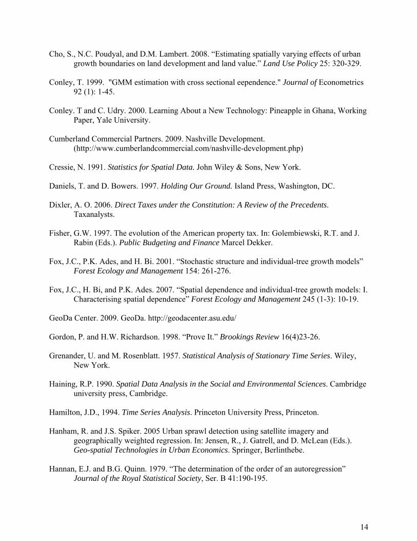
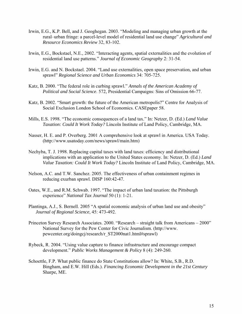
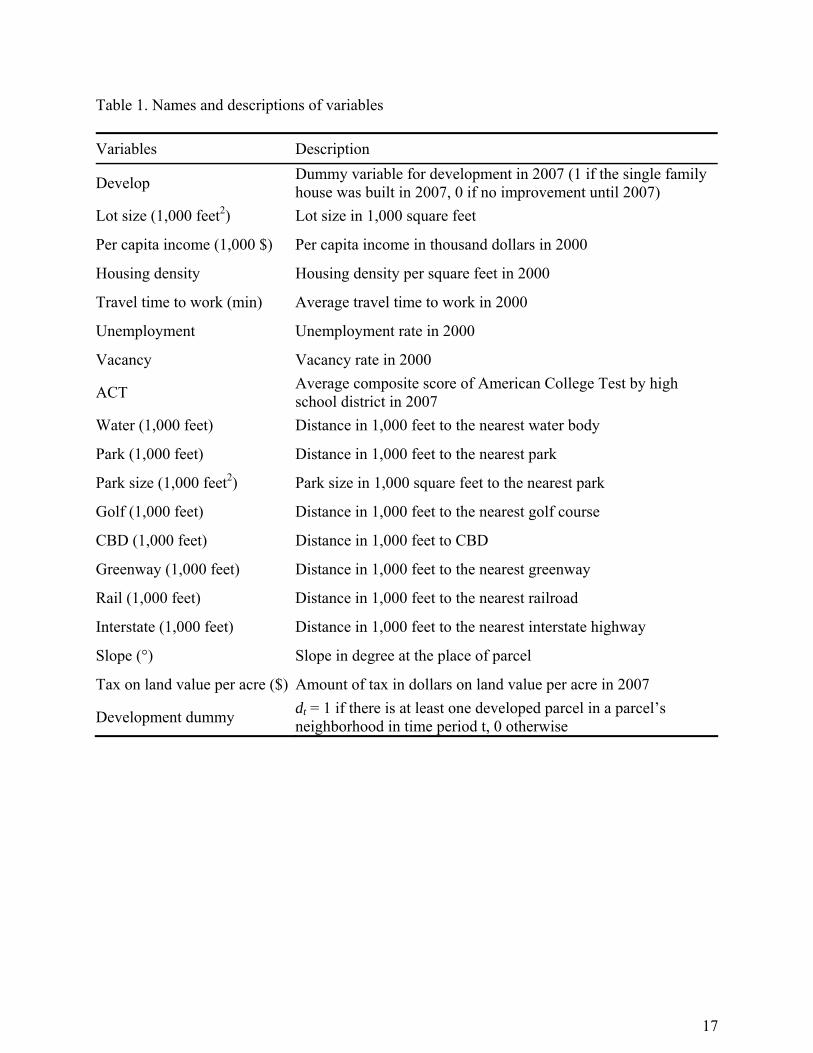
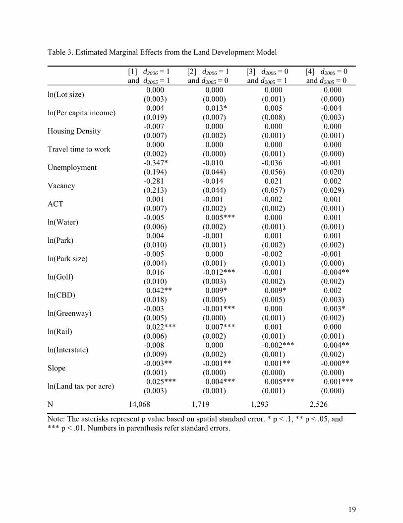
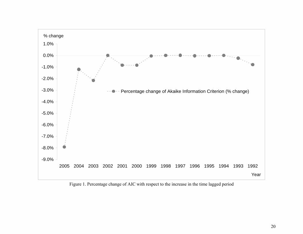
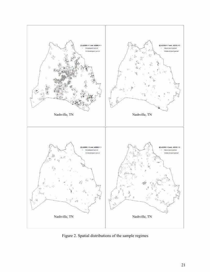
Nashville TN Nashville TN

Nashville TN Nashville TN

Figure 2 Spatial distributions of the sample regimes

21