Washington University in St. Louis Washington University in St. Louis

Washington University Open Scholarship Washington University Open Scholarship

Engineering and Applied Science Theses & Dissertations McKelvey School of Engineering

Spring 5-2017

Measuring Molecular Orientation and Rotational Mobility Using a Measuring Molecular Orientation and Rotational Mobility Using a

Tri-spot Point Spread Function Tri-spot Point Spread Function

Oumeng Zhang Washington University in St Louis

Follow this and additional works at: https://openscholarship.wustl.edu/eng_etds

Part of the Engineering Commons, and the Optics Commons

Recommended Citation Recommended Citation Zhang, Oumeng, "Measuring Molecular Orientation and Rotational Mobility Using a Tri-spot Point Spread Function" (2017). Engineering and Applied Science Theses & Dissertations. 226. https://openscholarship.wustl.edu/eng_etds/226

This Thesis is brought to you for free and open access by the McKelvey School of Engineering at Washington University Open Scholarship. It has been accepted for inclusion in Engineering and Applied Science Theses & Dissertations by an authorized administrator of Washington University Open Scholarship. For more information, please contact digital@wumail.wustl.edu.

WASHINGTON UNIVERSITY IN ST. LOUIS

School of Engineering and Applied Science

Department of Computer Science and Engineering

Thesis Examination Committee:

Matthew D. Lew

Joseph A. O’Sullivan

Lan Yang

Measuring Molecular Orientation and Rotational Mobility

Using a Tri-spot Point Spread Function

by

Oumeng Zhang

A thesis presented to the School of Engineering

of Washington University in St. Louis in partial fulfillment of the

requirements for the degree of

Master of Science

May 2017

Saint Louis, Missouri

ii

Contents List of Figures .................................................................................................................................................. iii Acknowledgments ........................................................................................................................................... iv Dedication .......................................................................................................................................................... v Abstract .............................................................................................................................................................. vi 1 Background ................................................................................................................................................. 1 1.1 State Transitions of Single Molecules ............................................................................................. 2 1.2 Molecular Orientation ....................................................................................................................... 4 1.3 Scope of Dissertation ........................................................................................................................ 5 2 Designing a Tri-spot PSF for Molecular Orientation Estimation .............................................. 7 2.1 Point Spread Function Design ......................................................................................................... 7 2.1.1 Intensity Distribution at Image Plane for Dipole Emitters ........................................... 7 2.1.2 Tri-spot PSF and Phase Mask Design ............................................................................14 2.1.3 Procedure for Mask Design ..............................................................................................16 2.2 Molecular Orientation Estimation Using Basis Inversion Method .........................................23 2.3 Molecular Orientation Estimation Using a Maximum Likelihood Estimator ........................25 2.3.1 Model for Quickly Rotating Single Molecule Emitters ................................................26 2.3.2 Design of a Maximum Likelihood Estimator ................................................................29 2.3.3 Evaluating Estimator Performance Using Simulated Images .....................................30 2.3.3.1 Analysis of Mean Orientation Estimation ......................................................31 2.3.3.2 Analysis and Tuning of Rotational Mobility Estimation .............................35 2.4 Summary ............................................................................................................................................38 3 Measuring the Orientation of Fluorescent Emitters Using Tri-spot PSF .............................40 3.1 PSF Evaluation Using Fluorescent Beads ....................................................................................41 3.1.1 Impact of Absorption Dipole Moments on Apparent Rotational Mobility .............41 3.1.2 Measuring Dipole Moments Using Basis Inversion .....................................................45 3.2 Measuring the Orientation of Single Fluorescent Molecules ....................................................48

iii

3.3 Summary ............................................................................................................................................53 4 Outlook .......................................................................................................................................................54 References ........................................................................................................................................................56

iv

List of Figures Figure 1-1: Simplified Jablonski diagram describing molecule-light interaction ....................................... 3 Figure 1-2: Absorption rate and emission pattern of a dipole emitter ....................................................... 4 Figure 2-1: Overview of the imaging system and coordinate system .......................................................10 Figure 2-2: Back focal plane intensity distribution for different molecular orientations .......................11 Figure 2-3: Bisected PSF and quadrated PSF ...............................................................................................15 Figure 2-4: Different partition shapes and the corresponding PSF and precision .................................18 Figure 2-5: Different phase ramp orientations and the corresponding PSF ...........................................19 Figure 2-6: Sensitivity to a certain term of molecular orientation .............................................................20 Figure 2-7: Basis images of back focal plane and image plane ..................................................................22 Figure 2-8: New partition to enhance sensitivity to a certain term of molecular orientation ...............22 Figure 2-9: Image partitioning for signal and background photon counting ..........................................25 Figure 2-10: Axis rotation to calculate second moments of molecular orientation ................................27 Figure 2-11: One example of estimation using the maximum likelihood estimator ..............................30 Figure 2-12: Precision of the maximum likelihood estimator ....................................................................33 Figure 2-13: Accuracy of the maximum likelihood estimator ....................................................................34 Figure 2-14: Rotational mobility estimation distribution ............................................................................35 Figure 2-15: Rotational mobility estimation bias under different signal to background ratio ..............36 Figure 2-16: Parameter for rotational mobility tuning curve .....................................................................37 Figure 2-17: Rotational mobility tuning curve verification .........................................................................38 Figure 3-1: Different between apparent and true rotational mobility due to pump anisotropy ...........44 Figure 3-2: Raw image of fluorescent beads .................................................................................................46 Figure 3-3: Estimation result of one fluorescent beads ..............................................................................46 Figure 3-4: Distribution of dipole moments of fluorescent beads ............................................................47 Figure 3-5: Raw image of single-molecule emitters .....................................................................................49 Figure 3-6: Distribution of rotational mobility of single-molecule emitters ............................................49 Figure 3-7: Orientation measurements of two single-molecule emitters .................................................50 Figure 3-8: Localization bias while moving molecule along optical axis ..................................................52

v

Acknowledgments I would like to thank my research advisor, Dr. Matthew D. Lew, who has spent a lot of his time

teaching me related background knowledge and experimental techniques, helping me improving my

research skills, and pointing me to the right direction of this thesis. Without his kindness and patience,

I could not have completed this work.

I would also like to thank my labmates, Tianben Ding and Jin Lu, who helped me with the experiment

setup and sample preparation, and Hesam Mazidi, who helped me improving the performance of the

estimation algorithm. It has been a great pleasure working in this lab, and I am looking forward to

keep working with them during my Ph.D.

Oumeng Zhang

Washington University in St. Louis

May 2017

vi

Dedicated to my parents.

vii

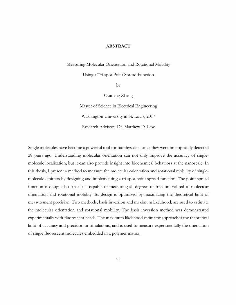
ABSTRACT

Measuring Molecular Orientation and Rotational Mobility

Using a Tri-spot Point Spread Function

by

Oumeng Zhang

Master of Science in Electrical Engineering

Washington University in St. Louis, 2017

Research Advisor: Dr. Matthew D. Lew

Single molecules have become a powerful tool for biophysicists since they were first optically detected

28 years ago. Understanding molecular orientation can not only improve the accuracy of single-

molecule localization, but it can also provide insight into biochemical behaviors at the nanoscale. In

this thesis, I present a method to measure the molecular orientation and rotational mobility of single-

molecule emitters by designing and implementing a tri-spot point spread function. The point spread

function is designed so that it is capable of measuring all degrees of freedom related to molecular

orientation and rotational mobility. Its design is optimized by maximizing the theoretical limit of

measurement precision. Two methods, basis inversion and maximum likelihood, are used to estimate

the molecular orientation and rotational mobility. The basis inversion method was demonstrated

experimentally with fluorescent beads. The maximum likelihood estimator approaches the theoretical

limit of accuracy and precision in simulations, and is used to measure experimentally the orientation

of single fluorescent molecules embedded in a polymer matrix.

1

Chapter 1

Background

Since the first optical detection of a single molecule 28 years ago [1], single-molecule imaging has

become a powerful tool for gaining insight into the biochemical activities in living cells [2]. Optical

imaging with resolution beyond the diffraction limit can be achieved by localizing single fluorescent

molecules attached to biological structures [3]–[6]. Measuring the orientation of single-molecule

emitters has become an interesting topic recently. Not only can it improve the localization accuracy

by estimating the localization bias due to orientation effects [7]–[9], orientation information is also

helpful for understanding biochemical activities such as DNA bending and tangling [10], or

transbilayer lipid motion within cell membranes [11]. Variants of methods measuring molecular

orientation and rotational mobility has been introduced to the field including modeling the emission

pattern of a single-molecule emitter [12]–[15] or tuning the excitation polarization [10], [16], [17].

However, they either require complicated optical instruments or do not have enough sensitivity to

measure both the 3D molecular orientation and rotational mobility of single molecules simultaneously.

This thesis describes my contributions to developing a method for measuring all degrees of freedom

related to molecular orientation and rotational mobility that can be easily implemented on fluorescent

microscopes.

2

This Chapter introduces background material related to this thesis. In Section 1.1, I will introduce the

basics of how a fluorescent molecule interacts with light. In Section 1.2, I will introduce molecular

orientation and how it affects light-molecule interactions.

1.1 State Transitions of Single Molecules In fluorescence microscopy, we use light to excite fluorescent molecules when they are in an emissive

form as shown in Fig. 1-1. In this process, a photon from incident light is absorbed by the molecule.

The energy within the photon causes the molecule to undergo a transition from the ground state (S0)

to an excited state (S1). After vibrational relaxation within a few picoseconds, the molecule relaxes

back to the ground state, with a photon emitted simultaneously [18]. The typical excited state lifetime,

or the time the molecule spends in the S1 state before emitting a photon, is on the order of

nanoseconds. The emitted photon’s wavelength is red-shifted since energy is lost as the molecule

relaxes vibrationally. The emission occurs much faster compared to the exposure time of one camera

frame, so a conventional camera captures multiple fluorescence photons within one frame. The

transition from excited state to ground state can also occur via non-radiative pathways; this energy is

released through heat instead of light.

While a molecule is in the excited state, it is possible for the spin of the electron to be flipped, causing

the molecule to enter a triplet state (T1). The molecule can stay in the triplet state from milliseconds

to minutes, which is comparable with the exposure time. While in this state, the molecule does not

interact with the excitation light. Therefore, the molecule will appear to be “dark” on the camera.

3

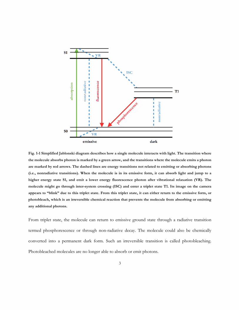
Fig. 1-1 Simplified Jablonski diagram describes how a single molecule interacts with light. The transition where

the molecule absorbs photon is marked by a green arrow, and the transitions where the molecule emits a photon

are marked by red arrows. The dashed lines are energy transitions not related to emitting or absorbing photons

(i.e., nonradiative transitions). When the molecule is in its emissive form, it can absorb light and jump to a

higher energy state S1, and emit a lower energy fluorescence photon after vibrational relaxation (VR). The

molecule might go through inter-system crossing (ISC) and enter a triplet state T1. Its image on the camera

appears to “blink” due to this triplet state. From this triplet state, it can either return to the emissive form, or

photobleach, which is an irreversible chemical reaction that prevents the molecule from absorbing or emitting

any additional photons.

From triplet state, the molecule can return to emissive ground state through a radiative transition

termed phosphorescence or through non-radiative decay. The molecule could also be chemically

converted into a permanent dark form. Such an irreversible transition is called photobleaching.

Photobleached molecules are no longer able to absorb or emit photons.

4

1.2 Molecular Orientation The orientation of a single molecule affects how it interacts with light. Here I provide a simple

introduction on how absorption and emission are affected by molecular orientation. A more detailed

treatment can be found in [19].

We denote the orientation of a molecule with a unit vector µ , which characterizes the transition

dipole moment of the molecule. The rate that the molecule transitions from ground state to the excited

state is related to the excitation electric field E [20]:

2excitationG µ ×Eµ (1-1)

In eq. 1-1, we assume the electric field is constant within the dimension of a single-molecule emitter

(a few nm). The excitation rate is proportional to 2cos n , where n is the angle between the transition

dipole moment and the excitation electric field as shown in Fig. 1-2a.

Fig. 1-2 (a) The absorption rate of a fluorescent molecule has a cosine-squared dependence on the angle between

the excitation electric field and the dipole moment; (b) The emission intensity of a dipole at far field has a sine-

squared dependence on the angle between the emission direction and the dipole moment.

5

The emission pattern of a single-molecule emitter can be calculated by solving the electromagnetic

wave equation. In the far field (the distance to the emitter r is much larger than the wavelength), the

emission intensity is given by [19]:

2

_ 1far fieldU µ - ×rr

µ (1-2)

According to eq. 1-2, the emission intensity is proportional to 2sin h , where h is the angle between

the transition dipole moment and the emission direction.

Various methods have been developed to measure the orientation by either measuring excitationG or

_far fieldU . One thing to notice is that the excitation transition dipole moment could be different from

the emission transition dipole moment [21]. The method I introduce in this thesis is based on

measuring the distribution of _far fieldU , and is therefore optimized for measuring the emission dipole

moment. Therefore, the molecular orientation mentioned in this thesis refers to the emission dipole

moment if not specified otherwise. In Chapter 3, I will briefly introduce how absorption dipole

moment affects this method.

1.3 Scope of this Dissertation The remainder of this thesis includes a new method using a tri-spot point spread function (PSF) to

estimate molecular orientation and rotational mobility of single-molecule emitters. In Chapter 2, I

introduce the design and optimization of the PSF. The tuning of the maximum likelihood estimator

6

is also introduced in this chapter. Chapter 3 includes a set of experiments with various non-biological

fluorescent samples to characterize the performance of this PSF.

7

Chapter 2

Designing a Tri-spot Point Spread Function for Molecular Orientation and Rotational Mobility Estimation

This chapter introduces a tri-spot point spread function for measuring molecular orientation and

rotational mobility.

This chapter is organized as follows: In Section 2.1, I will introduce optical Fourier processing [22]

and how the mask was designed based on a theoretical framework for optimizing its measurement

performance. Optimization of the mask is also discussed in this section. In Section 2.2, I present a

maximum likelihood estimator for evaluating the performance of this PSF using simulated data.

2.1 Point Spread Function Design

2.1.1 Intensity Distribution at Image Plane for Dipole Emitters It is important to understand the relation between molecular orientation and the image captured by

the camera before designing a method to estimate molecular orientation and rotational mobility. We

model the emitter as an oscillating electric dipole with an orientation parameterized by a unit vector

µ given by

8

sin cossin sincos

x

y

z

µ q fµ q fµ q

é ù é ùê ú ê ú= =ê ú ê úê ú ê úë û ë û

µ (2-1)

where xµ , yµ , and zµ denote the projection of µ onto each Cartesian axis as shown in Fig. 2-1a.

We can also use the polar angle q and azimuthal angle f to represent this vector. Since µ describes

a dipole, the domain of definition is a hemisphere. We set , [ 1,1]x yµ µ Î - , [0,1]zµ Î , or

[0, / 2],q pÎ [0,2 ]f pÎ .

The electric field distribution can be calculated by solving Maxwell’s equations. After the ray rotation

effect of the objective lens, the electric field distribution at the back focal plane (bfp) can be written

using the Green’s tensor ( , )bfp rFG [19], [22] :

1 12 1/2

0

2 2 2 2

2 2 2 2

exp( )( , )

4 (1 )

sin ( ) cos ( ) 1 sin(2 )( 1 1) / 2 cos( )

sin(2 )( 1 1) / 2 cos ( ) sin ( ) 1 sin( )0 0 0

objbfp

obj

in kf nf n

rp r

r r r

r r r

F =-

é ùF + F - F - - - Fê úê ú´ F - - F + F - - Fê úê úë û

G

(2-2)

In eq. 2-2, { , }rF are the polar coordinates of the back focal plane as shown in Fig. 2-1.

max 1/NA nr = is determined by the numerical aperture of the objective lens. 0n and 1n denote the

reflective indices of the back focal plane (normally 0 1n » ) and of the medium in which the emitter is

embedded.

9

Notice that since the propagation direction is parallel to the optical (z) axis, there is no z component

in bfpG . The back focal plane electric field is thus given by [19]:

21( , , ) exp( 1 ) ( , )bfp bfpE d A in kdr r rF = - FG µ (2-3)

where d is the defocus distance of the sample from the focal plane of the imaging system.

In order to detect the polarization of the electric field, our imaging system separates the x- and y-

polarized emission light into different channels. The back focal plane intensity distribution for x- and

y-polarized light can be calculated as:

2

, 1 ,

2, 1 ,

( , , ) exp( 1 ) ( , )

( , , ) exp( 1 ) ( , )

bfp x bfp x

bfp y bfp y

E d A in kd

E d A in kd

r r r

r r r

F = - F

F = - F

G

G

µ

µ (2-4)

,bfp xG and ,bfp yG refer to the first and second rows of bfpG , so unlike bfpE , , ( )bfp x yE are scalars instead

of vectors. The x- and y-polarized back focal plane intensity distributions are given by

2

, ( ) , ( )bfp x y bfp x yI E= , and the total intensity when both channels are combined is given by

2

, ,bfp bfp bfp x bfp yI I I= = +E . The intensity distributions bfpI and ,bfp xI for certain µ orientations are

shown in Fig. 2-2.

10

Fig. 2-1 (a) Overview of the imaging system and coordinate system for the orientation of molecules in object

space. Note that since 𝒇𝒕𝒖𝒃𝒆 is much larger than the pupil radius, the paraxial approximation in Fourier optics

is applicable when analyzing the light propagation from the back focal plane to image plane; (b) Overview of

polarization sensitive 4f system [23] created by Dr. Matthew D. Lew. The beam splitter (PBS) separates light

into x- and y- polarized light. The first lens of the 4-f system creates an image of the pupil plane within the

objective lens on the spatial light modulator (SLM). The SLM adds a phase delay pattern to the electric field

distribution. The second lens of the 4-f system creates an image plane on the CMOS camera conjugate to the

intermediate image plane created by the microscope. The x- and y- polarized images are captured by different

regions of the CMOS camera so that both can be captured simultaneously.

11

Fig. 2-2 Back focal plane intensity distribution for different molecular orientations. The numerical aperture of

the objective lens is 1.4 and the refractive index is 1.52. (a) x- and y- polarized combined back focal plane intensity

distribution; (b) Back focal plane intensity distribution of only x-polarized light.

12

The electric field at the back focal plane after adding certain masks ( , )xy rF and ( , )yy rF to both

polarization channels can be written as:

, ( ) (, ) )( ex ( ( , )' p )bfp x ybfp x y x yEE iy r= F (2-5)

Note that ( , )xy rF and ( , )yy rF can represent either amplitude, phase, or complex modulation.

The electric field at the imaging plane is simply the Fourier transform of the electric field at the back

focal plane:

, ( ), ( ) ( ) ', { },img bfp xx yyE ' ' d ECrF = F (2-6)

where F denotes the two-dimensional Fourier transform and C is a complex constant. We define:

0max2 1/2

( ) 1

, ( )

'cos( )2( , ) (1 )

, ( )0 0

( , , )

( , ) x y tube

img x y

ikn 'i fin kd

bfp x y

' ' d

C e e e d drrrp

y r r

r

r r rF -F

F -

F

= F Fò ò

G

G (2-7)

This function can only be calculated numerically. We can write the results in the form:

, ( ) , ( ) , ( ) , ( )[ ( , , ) ( , , ) ( , , )]img x y x x y y x y z x yg ' ' d g ' ' d g ' ' dr r r= F F FG (2-8)

where , ( )i x yg denotes the contribution of dipole component iµ to the x(y)-polarized electric field.

The electric field distribution within the imaging plane can be simplified as:

, ( ) , ( ) ( , , )img x y img x yE A ' ' dr= FG µ (2-9)

The intensity distribution of electric field within the imaging plane can therefore be calculated as:

13

22, ( )

( )2 2

( ), ( )22 ( )* 2

, ( ), ( ) , ( ) , ( ) 0

*, ( ) , ( )*, ( ) , ( )*, ( ) , ( )

2 ( )2 ( )2 ( )

T

x x yx yx

x yy x y y

x yzz x yimg x y img x y img x y

x yx x y y x y

x zx x y z x y

y zy x y z x y

g XXYYgZZ

gI E E A I

g gg gg g

µµµµ µµ µµ µ

é ùé ùê úê úê úê úê úê úê ú

= = =ê úê úê úê ú

 ê úê úê úê úÂê úê ú ë ûÂê úë û

2

2

2

( )

( )

( )

T

x

y

z

x y x y

x y x z

x y y z

XYXZYZ

µµµµ µµ µµ µ

é ù é ùê ú ê úê ú ê úê ú ê úê ú ê úê ú ê úê ú ê úê ú ê úê ú ê úë û ë û

(2-10)

We consider ( ) ( ) ( )[ ,..., ]x y x y x yXX YZ=B as the basis images of the system. These basis images are

independent of the emitter and would only change if there are some changes in the imaging system.

If the emitter is rotating, the image becomes a temporal average of multiple orientations, and the

intensity at the imaging plane becomes:

2,

2,

2,0

, ( ) ( ), ,0

, ,

, ,

( )( )( )

( ) ( )( ) ( )( ) ( )

x

yt

zimg x y x y

x y

x z

y z

II dt

t

t

t

t t

t t

t t

µ tµ tµ t

tµ t µ tµ t µ tµ t µ t

é ùê úê úê úê ú=ê úê úê úê úë û

òB (2-11)

where t is the exposure time of one camera frame. The subscript t is used to indicate that this

variable is a function of time t , which maintained for the rest of this thesis. We use × to denote the

temporal average of a function, and thus eq. 2-11 can be written as:

2 2 2

, ( ) 0 ( ) , , , , , , , , ,

0 ( )

, , , , ,T

img x y x y x y z x y x z y z

x y

I I

It t t t t t t t tµ µ µ µ µ µ µ µ µé ù= ë û

=

B

B M (2-12)

14

We use M as the second-moment matrix describing molecular orientation dynamics during a single

camera frame. For a given imaging system, the image is the linear combination of all 12 basis images

(2 polarizations and 6 basis images per polarization). The intensity of each basis is proportional to the

second moment of the molecular orientation; that is, the images created by the imaging system in

response to electric dipoles with second moments vector M . For example, an isotropic emitter has

second moments [ ]1/ 3,1/ 3,1/ 3,0,0,0 TM = , and a fixed emitter has second moments

2 2 2, , , , ,T

x y z x y x z y zµ µ µ µ µ µ µ µ µé ùë ûM = .

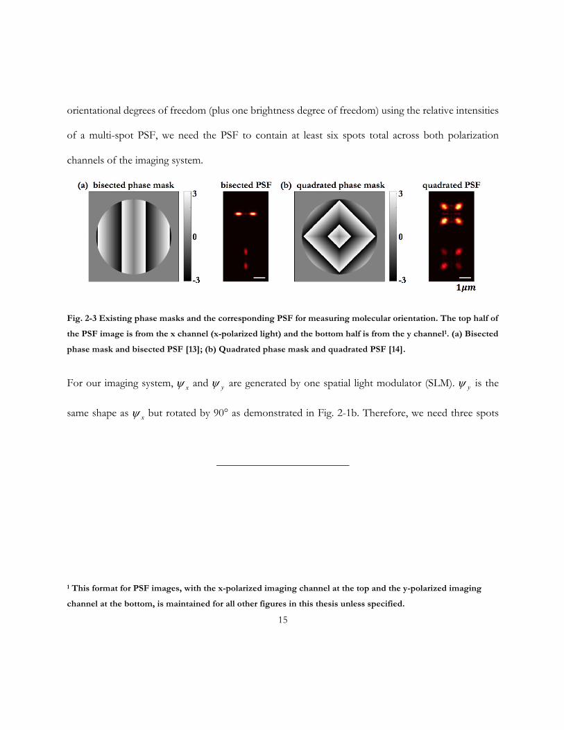
2.1.2 Tri-spot Point Spread Function and Phase Mask design Existing methods such as the bisected PSF [13] and the quadrated PSF [14] use the relative intensity

of each spot within the PSF to estimate the molecular orientation as shown in Fig. 2-3. For single-

molecule emitters, the total photon budget is limited. Therefore, the shape of the PSF should be as

concentrated as possible. Separating emission light into more spots would lower the signal-to-

background ratio (SBR), which will affect the precision of the orientation measurement. On the other

hand, separating emission light into fewer spots could introduce degeneracy into the measurement

such that certain orientations become unresolvable from one another.

As we discussed in Section 2.1.1, the image of a fluorescent emitter is a function of the second

moments M of its dipole orientation distribution. Since 2 2 2 2 2 2, , , , , ,x y z x y zt t t t t tµ µ µ µ µ µ+ + = + +

1= due to the definition of µ in eq. 2-1, there are a total five degrees of freedom to describe

molecular orientation and rotational mobility of a single-molecule emitter. To estimate all 5

15

orientational degrees of freedom (plus one brightness degree of freedom) using the relative intensities

of a multi-spot PSF, we need the PSF to contain at least six spots total across both polarization

channels of the imaging system.

Fig. 2-3 Existing phase masks and the corresponding PSF for measuring molecular orientation. The top half of

the PSF image is from the x channel (x-polarized light) and the bottom half is from the y channel1. (a) Bisected

phase mask and bisected PSF [13]; (b) Quadrated phase mask and quadrated PSF [14].

For our imaging system, xy and yy are generated by one spatial light modulator (SLM). yy is the

same shape as xy but rotated by 90° as demonstrated in Fig. 2-1b. Therefore, we need three spots

1 This format for PSF images, with the x-polarized imaging channel at the top and the y-polarized imaging

channel at the bottom, is maintained for all other figures in this thesis unless specified.

16

within each channel in order to get enough information and achieve good SBR at the same time.

Consequently, we designed a mask that divides the back focal plane into three partitions. Each

partition has different linear phase ramp, which bends light within that partition like a prism. After

the Fourier transform operation of the final lens in the 4-f system, the light from each partition is

focused and translated onto separate regions of the camera. Therefore, the PSF within each channel

of the imaging plane contains three spots, which is why this new PSF is called the tri-spot PSF. The

optimization of the shape, size and phase ramp direction of each partition will be discussed in the

following section.

2.1.3 Procedure for Mask Design To achieve highly precise estimates of molecular orientation, we calculate the Fisher information (FI)

[24] content of masks whose partitions vary in shape and size. We use the Cramér-Rao lower bound

(CRLB), which is the inverse of the Fisher information matrix, to evaluate the performance of each

partition method, because it gives us the theoretical lower bound of the variance of any unbiased

estimator.

For simplicity, we only evaluate the CRLB of fixed dipole orientation distributions and use these to

optimize the mask design, i.e., 2 2, , ,,...,x x y z y zt t tµ µ µ µ µ µ= = . The rotational mobility estimation

capabilities of the mask will be evaluated in Chapter 3.

Since we are using the integrated intensity of six spots from both channels for estimation, we write

the intensity as 1 6( , ) [ ,..., ]x y I Iµ µ =I . The Fisher information matrix is calculated as [25]:

17

2

6

1 2

( ) ( )( )1( )

( )( ) ( )

i i i

x x y

i i i ii i

x y y

I I I

I I II b

µ µ µ

µ µ µ=

¶ ¶ ¶é ùê ú¶ ¶ ¶ê ú=ê ú¶ ¶ ¶+ê ú¶ ¶ ¶ê úë û

åFI (2-13)

where 1 6,...,b b in eq. 2-13 denote the total background photons within each spot. The CRLB is simply

the inverse of the FI matrix:

1~

~x

y

CRLB

CRLBµ

µ

-é ù

= = ê úê úë û

CRLB FI (2-14)

Since the distributions of x

CRLBµ and y

CRLBµ are symmetric due to the circular symmetry of the

optical system, x

CRLBµ is enough for evaluating the precision of the PSF. Several different phase

mask designs, the corresponding PSFs when the molecular orientation is 2x yµ µ= = , and the

corresponding x

CRLBµ with 20,000 photons to 20 photon/pixel SBR are shown in Fig. 2-4.

The first design in Fig. 2-4a is based on the back focal plane intensity distribution before polarization

separation as shown in Fig. 2-2a. The back focal plane intensity distribution has a donut shape. The

hole of the donut shifts outward as q increases and rotates as f changes (q and f can be converted

to xµ and yµ using eq. 2-1). Therefore, we expect that by separating the light within the inner circle

from light in the outer ring of the back focal plane, we can obtain more precise measurements of q .

The x

CRLBµ results in Fig. 2-4a show that this partition can achieve high precision for xµ estimation.

The CRLB is lower than 4.6×10-4, which implies the standard deviation of the estimator could be as

low as 0.02 for all molecular orientations under this SBR.

18

Fig. 2-4 Different partition shapes of the trisected phase mask and the corresponding PSFs and theoretical lower

bounds of estimation precision. Figures in the right column show the 2D map of the 𝑪𝑹𝑳𝑩𝝁𝒙 distribution vs.

the x-y projection of 𝝁 (a hemisphere). (a) Donut pattern phase mask partition; (b)(c)(d) Different shapes of

vertical-stripe shape phase mask partition.

19

However, since the back focal plane intensity distribution after separating polarizations becomes

vertical stripes in the x channel (and horizontal stripes in the y channel, see Fig. 2-2), the ring-shape

partition is not optimal for sensing changes in molecular orientation using a polarization-sensitive

imaging system. We tested different vertical stripe patterns as shown in Fig. 2-2b~d, and the shape in

2-2c has the smallest CRLB, which means this mask provides the best precision among these masks

with vertical partitions.

Fig. 2-5 Different phase ramp orientations and the corresponding PSFs in x channel for a fixed dipole emitter

𝝁 = [𝟎. 𝟔𝟑, 𝟎, 𝟎. 𝟕𝟖] (a) Spots within the PSF aligned in a line; (b) Spots within the PSF aligned in a triangle.

After deciding the partition pattern, we need to consider the phase ramp within each partition. The

direction of the phase ramp affects the location of each spot on the imaging plane, and the slope

affects how far each spot is pushed away from the center of the PSF. As shown in Fig. 2-5, for certain

molecular orientations, arranging three spots of the PSF in a line would cause possible localization

confusion when only two adjacent spots are bright enough to be detected. Arranging three spots in a

triangular shape solves this problem.

20

However, the mask from Fig. 2-5b produces a PSF that has the same intensity distribution for certain

molecular orientations, for example, when 0zµ = . The PSF corresponding to molecular orientations

[ , ]x yµ µ± (or [ , ]x yµ µ± ) are very similar to each other as shown in Fig. 2-6a.

Fig. 2-6 Tri-spot mask and PSF before and after enhancing 𝝁𝒙𝝁𝒚 sensitivity. (a) Before enhancing 𝝁𝒙𝝁𝒚

sensitivity, the images of an emitter with molecular orientations [𝝁𝒙, ±𝝁𝒚] appear very similar in the image

plane; (b) After enhancing 𝝁𝒙𝝁𝒚 sensitivity, these two cases are distinguishable.

To understand this phenomenon, we need to analyze the back focal plane intensity distribution.

21

According to eq. 2-4, we can calculate the intensity distribution at back focal plane for an in-focus

single-molecule emitter as:

, ( )

, ( )

, ( )2, ( )

, ( )

, ( )

, ( )

XX x y

YY x y

ZZ x ybfp x y

XY x y

XZ x y

YZ x y

BFPBFPBFP

I ABFPBFPBFP

é ùê úê úê ú

= ê úê úê úê úê úë û

M (2-15)

The back focal plane intensity distribution is a linear combination of 6 basis back focal plane images,

as shown in Fig. 2-7a. If we use the phase mask shown in Fig. 2-5b, the XYBFP basis would have zero

total intensity within each partition due to the symmetric distribution. Therefore, the image basis XY

would contribute zero total photons to each spot region in the image as well. In other words, this

mask has no sensitivity to measure the x yµ µ term, so the orientation pair [ , ]x yµ µ± (or [ , ]x yµ µ± ) is

not distinguishable using the relative intensity of each spot.

Since the energy is concentrated at the corners of XYBFP basis, we combine the shapes in Fig. 2-8b

and 2-8a, which is the original vertical partition shape, to add x yµ µ sensitivity to the current mask.

We add the black region of Fig. 2-8b to the black region of Fig. 2-8a, and the white region of Fig. 2-

8b to the white region of Fig. 2-8a to get a final partition configuration shown in Fig. 2-8c. Now that

the PSF is sensitive to the x yµ µ term, the orientation pair [ , ]x yµ µ± (or [ , ]x yµ µ± ) is now

distinguishable as shown in Fig. 2-6b. The basis images of the mask shown in Fig. 2-6b are shown in

Fig. 2-7b.

22

Fig. 2-7 Basis images of back focal plane and image plane. (a) Back focal plane basis images; (b) Image plane

basis images after adding the optimized tri-spot phase mask in Fig. 2-6b at the back focal plane.

Fig. 2-8 Enhancing 𝝁𝒙𝝁𝒚 sensitivity of the tri-spot mask. (a) Vertical stripe partitions. Light within the black

region is pushed downward, while light within the white region is diverted to the sides; (b) A partition that

pushes light within 4 corners of the back focal plane downward (black) or to the side (white); (c) a mask that

combines the white and black regions within (a) and (b).

23

2.2 Molecular Orientation Estimation Using Basis Inversion

We write the total photons within each spot as a vector 1 2 3 1 2 3[ , , , , , ]Tspot x x x y y yI I I I I I=I . Spots 1x ,

…, 3y are defined as shown in Fig. 2-7b.

We can denote the total photons within each spot of the six basis images as vectors; for example, the

XX basis has a spot vector 1 3[ ,..., ]Tspot x yXX XX=XX , etc. Now we can write eq. 2-11 as:

1 1 1 1 1 1

2 2 2 2 2 2

3 3 3 3 3 30 0

1 1 1 1 1 1

2 2 2 2 2 2

3 3 3 3 3 3

x x x x x x

x x x x x x

x x x x x xspot spot

y y y y y y

y y y y y y

y y y y y y

XX YY ZZ XY XZ YZXX YY ZZ XY XZ YZXX YY ZZ XY XZ YZ

I IXX YY ZZ XY XZ YZXX YY ZZ XY XZ YZXX YY ZZ XY XZ YZ

é ùê úê úê ú

= =ê úê úê úê úê úë û

I M B M (2-16)

spotB is a six-by-six matrix characterizing the response of the imaging system (i.e., its PSF). For our

optimized mask,

0.21 0.01 0.11 0.04 0.24 0.020.24 0.01 0.12 0.03 0.24 0.030.52 0.01 0.10 0.06 0.00 0.00

( )0.01 0.21 0.11 0.04 0.02 0.240.01 0.24 0.12 0.03 0.03 0.240.01 0.52 0.10 0.06 0.00 0.00

spotB AU

- -é ùê ú- -ê úê ú

= ê ú- -ê úê úê ú

-ë û

(2-17)

24

The columns of spotB are normalized by the total intensity of the brightest basis images, xXX and

yYY . Each column of spotB is linearly independent, which indicates a one-to-one correspondence of

the image intensity distribution spotI with the second moments of molecular orientation M .

The procedure to count the photons within each spot of an experimental image or the basis images is

as follows: We upsample the raw image by 10 times using Matlab function “kron”. An example of 2

times upsampling is given in eq. 2-18,

1 1 2 21 2 1 1 2 23 4 3 3 4 4

3 3 4 4

Þ (2-18)

The partitioning regions used to assign photons to each element of 1 2 3 1 2 3[ , , , , , ]Tspot x x x y y yI I I I I I=I

is shown in Fig. 2-9. Note that there is a 0th order bright spot in the center of the tri-spot PSF in

experimental images (see Section 3.1.2) that is not part of its design. This “leakage” of the standard

PSF into the experimental image is most likely due to imperfect phase modulation by the SLM in our

imaging system. Therefore, we set the phase ramps within the tri-spot PSF mask to push the spots far

away from the center (see Fig. 2-6b) for experimental images. This spacing allows our image analysis

algorithm to separate the 0th order spot (by using a 10-pixel radius circle) from the rest of the tri-spot

PSF. We calculate the average photons per pixel within region A as the background for a given

channel, denoted as ( ),1,...,3x yb . After subtracting the background photon level from each pixel (which

25

is not required for simulated images without background), the total photons within regions B, C, and

D are assigned as the signal for a given channel, denoted as ( ),1,...,3x ys .

Fig. 2-9 Image partitioning for signal and background photon counting (unit: pixel before upsampling). (a)

Partitioning for simulated images; (b) Partitioning for experimental images.

Since eq. 2-16 already provides the relation between the image intensity distribution and the second

moments of molecular orientation, we can simply invert the basis matrix and calculate the second

moments of molecular orientation as 10/spot spot I

-=M B s , where 1 3[ ,..., ]Tspot x ys s=s and 0I is a scaling

factor as defined in eq. 2-10.

2.3 Molecular Orientation Estimation Using a Maximum Likelihood Estimator

To test the performance of the tri-spot PSF, we built an estimator and tested it with simulated images.

A general linear estimator is based on basis matrix inversion, as described in the previous section.

However, this method is affected by photon shot noise, and the precision will therefore suffer.

26

Consequently, we built an estimator based on a simplified forward model with fewer parameters that

describe molecular orientation and rotational mobility.

2.3.1 Model for Quickly Rotating Single-Molecule Emitters Consider a mobile dipole , , ,[ , , ] [sin ( )cos ( ),sin ( )sin ( ),cos ( )]T T

x y zt t t t t t t t tµ µ µ q t f t q t f t q t= =µ

that rotates around a certain mean orientation [ , , ] [sin cos ,sin sin ,cos ]T Tx y zµ µ µ q f q f q= =µ over

time t . We assume that the rotation is much faster than the acquisition time t of one camera frame,

which implies ergodicity. There exists an orientation distribution probability density function

, ( , )Pt tq f t tq f so that the temporal average of tµ is equal to the spatial orientation average over this

distribution. We assume that the distribution is symmetric around the mean orientation µ . The

second moment of the molecular orientation can be calculated as:

2 /2

, , , , ,0 0

( , ) ( , ) ( , )sini j i j P d dt t

p p

t t t t t t t t q f t t t t tµ µ µ q f µ q f q f q q f= ò ò (2-19)

where , , ,i j x y z= in eq. 2-19.

To evaluate this integration, we need to rotate the mean orientation as shown in Fig. 2-10. First, rotate

about z axis by an angle f- , then rotate about y axis by an angle q- . After the rotation, the mean

orientation lies along the z axis. The relation between the dipole orientation before the rotation 'tµ

and after the rotation tµ is:

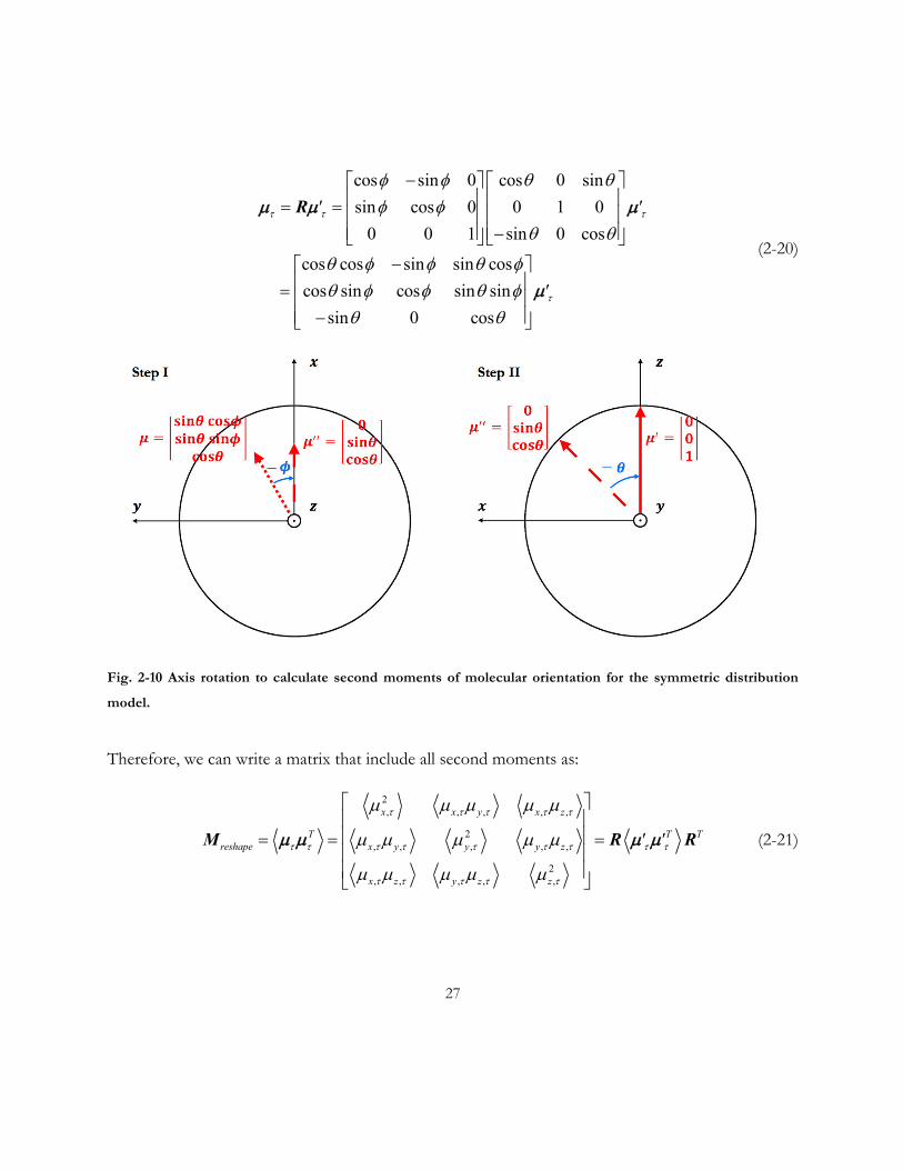
27

cos sin 0 cos 0 sinsin cos 0 0 1 00 0 1 sin 0 cos

cos cos sin sin coscos sin cos sin sinsin 0 cos

' '

'

t t t

t

f f q qf f

q q

q f f q fq f f q f

q q

-é ù é ùê ú ê ú= = ê ú ê úê ú ê ú-ë û ë û

-é ùê ú= ê úê ú-ë û

Rµ µ µ

µ

(2-20)

Fig. 2-10 Axis rotation to calculate second moments of molecular orientation for the symmetric distribution

model.

Therefore, we can write a matrix that include all second moments as:

2, , , , ,

2, , , , ,

2, , , , ,

x x y x z

T T Treshape x y y y z

x z y z z

' '

t t t t t

t t t t t t t t t

t t t t t

µ µ µ µ µ

µ µ µ µ µ

µ µ µ µ µ

é ùê úê ú= = =ê úê úë û

M R Rµ µ µ µ (2-21)

28

Since the mean orientation is rotated to 'µ , which is along z axis, and we already made an assumption

that the distribution of 'tµ is symmetric around 'µ , result of the integration of eq. 2-19 in the rotated

frame can be written as:

, , , , , ,

2 2, ,

0x y x z y z

x y

' ' ' ' ' '

' '

t t t t t t

t t

µ µ µ µ µ µ

µ µ l

= = =

= = (2-22)

Thus, we can calculate the second moments of the molecular orientation for this symmetric

distribution model as:

0 0

0 00 0 1 2

Treshape

ll

l

é ùê ú= ê úê ú-ë û

M R R (2-23)

By calculating the matrix multiplication, we have:

2 2, , ,

2 2, , ,

2 2, , ,

(1 ) / 3

(1 ) / 3

(1 ) / 3

x x x y x y

y y x z x z

z z y z y z

t t t

t t t

t t t

µ gµ g µ µ gµ µ

µ gµ g µ µ gµ µ

µ gµ g µ µ gµ µ

= + - =

= + - =

= + - =

(2-24)

where 1 3g l= - in eq. 2-24 denotes the rotational mobility of the molecule. A molecule’s rotational

mobility varies from 0 to 1. A completely fixed molecule will have 1g = , and an isotropic emitter

(freely rotating) will have 0g = . Now that both the molecular orientation and rotational mobility are

described by three parameters, xµ , yµ and g , we can test a maximum likelihood estimator based on

this model.

29

2.3.2 Design of a Maximum Likelihood Estimator We generate simulation images and add photon shot noise in Matlab as shown in Fig. 2-11b. The total

number of signal photons and total number of background photons within each spot region are

denoted as 1 3[ ,..., ]Tspot x ys s=s and 1 3[ ,..., ]Tspot x yb b=b . Since the second moments matrix of

molecular orientation M can be parameterized by xµ , yµ and g , the image intensity distribution can

be written as 0 0( , , , ) ( , , )spot x y spot x yI Iµ µ g µ µ g=I B M . Since photon detection is a Poisson process,

we can write the likelihood function as:

( ) ( )3

0, 1

( )( , , , )

( )!

ji ji ji jis b I bji ji

x yj x y i ji ji

I b el I

s bµ µ g

+ - +

= =

+=

+ÕÕ (2-25)

The log likelihood function is therefore given by

3

0, 1

( , , , ) ( ) ln( ) ( )x y ji ji ji ji ji jij x y i

I s b I b I bµ µ g= =

L µ + + - +åå (2-26)

After using MATLAB function fmincon to maximize 0( , , , )x yI µ µ gL , we obtain the estimation result

xµ , yµ and g . One example is shown in Fig. 2-11. Fig. 2-11a shows the ground truth images of a

molecule at a particular orientation, and Fig. 2-11c is generated using the estimated orientation

parameters from the noise perturbed image in Fig. 2-11b. The simulated noisy image agrees well with

the image generated from the estimated orientation parameters.

30

Fig. 2-11 Estimation using our maximum likelihood estimator. (a) Ground truth image without noise; (b) A

simulated image with Poisson noise, signal = 20,000 photons, background = 20 photon/pixel; (c) Recovered

image using after maximum likelihood estimation.

2.3.3 Evaluating Estimator Performance Using Simulated Images To evaluate the estimator performance, we simulated images of the tri-spot PSF with 20,000 signal

photons and 20 background photons/pixel. We choose the mean orientation domain x yµ µ´ =

[ 1: 0.1:1] [ 1: 0.1:1]- ´ - and 2 2 1x yµ µ+ < (Since CRLB is not defined at 1xµ = or 1yµ = ) and

{0 : 0.25 :1}g = . We generate 100 images for each ( , , )x yµ µ g combination. Other simulation

parameters are chosen to match our experiment setup, which will be introduced in Section 3.1.

31

2.3.3.1 Analysis of Mean Orientation Estimation We define the standard deviation of 100 estimations as estimation precision ,( )

x x eststd stdµ µ= , and

the difference between the mean of 100 estimations and the ground truth as estimation accuracy

, ,( )x x est x truebias meanµ µ µ= - . We calculated the precision of the estimator for all mean orientations

and plot this distribution in Fig. 2-12. The pattern of the standard deviation 2D map in Fig. 2-12a is

very similar to the x

CRLBµ pattern in Fig. 2-12b. The value of the standard deviation for most

orientations is within 1.5x

CRLBµ , thereby demonstrating that our estimator has nearly ideal

performance relative to the theoretical limit. The average /x x

std CRLBµ µ , which measures how

much worse our estimator’s precision is compared to the theoretical limit, among all orientations is

1.15 for {0.25,0.5,0.75}g = , and 1.08 for 1g = . The /x x

std CRLBµ µ distribution pattern is more

uniform for {0.5,0.75}g = (standard deviation less than 0.1), while there are certain orientations with

significantly worse than average performance for {0.25,1}g = .

The accuracy evaluation results are shown in Fig. 2-13. The absolute value of the bias (average of 100

estimations minus ground truth) is fairly small as shown in Fig. 2-13a. However, since we did 100

measurements for each orientation, the standard error of the estimation result should be:

1( )100x x

std bias CRLBµ µ= (2-27)

32

Therefore, if the estimator is accurate, the measured quantity /x x

bias CRLBµ µ should be mostly

confined to values within 3 ( ) / 0.3x x

std bias CRLBµ µ± = . There are a subset of orientations that

have bias larger than expected for {0.25,1}g = as shown in Fig. 2-13b. Even if we calculate

/x x

bias stdµ µ as shown in Fig. 2-12c, there is still a bias pattern in the 2D map. Since this bias is

invariant over multiple measurements at a fixed SBR, we can correct the bias of our estimator by using

Fig. 2-13 as a tuning map.

The above results show that this maximum likelihood estimator estimates the mean orientation more

accurately and precisely when g is neither too large nor too small before tuning. After the tuning and

bias correction, the estimator becomes unbiased.

33

Fig. 2-12 Precision of the maximum likelihood estimator using simulated images. (a) 2D map of the standard

deviation of 100 𝝁𝒙 estimates; (b) 2D map of the theoretical lower bound of precision for estimating 𝝁𝒙; and (c)

2D map of estimation precision compared to the theoretical limit.

34

Fig. 2-13 Accuracy of the maximum likelihood estimator. (a) Average estimation bias across 100 estimations; (b)

Estimation bias compared to the square root of CRLB; (c) Estimation bias compared to the standard deviation

among 100 estimations.

35

2.3.3.2 Analysis and Tuning of Rotational Mobility Estimation The histogram of estimated estg for several ground truth values trueg is shown in Fig. 2-14. The

distribution of estg is biased at 0trueg = . Since the range of estimated estg for our algorithm is

bounded so that [0,1]estg Î , the distribution of estimates is not Gaussian. Therefore, we define the

difference between the ground truth and the median over a set of measurements as the bias of the

estimator, instead of using the mean.

Fig. 2-14 Estimates of rotational mobility 𝜸 are biased for smaller values of 𝜸𝒕𝒓𝒖𝒆. The maximum values of 𝜸𝒆𝒔𝒕

are truncated since we set a bound of 𝜸𝒆𝒔𝒕 ∈ [𝟎, 𝟏] within the estimation algorithm. There is a peak at 𝜸𝒆𝒔𝒕 = 𝟏

for 𝜸𝒕𝒓𝒖𝒆 = 𝟏.

36

To characterize the relation between ( )est truebias meang g g= - and the signal-to-background ratio, we

simulated images of emitters at various SBRs as shown in Fig. 2-15. The exponential curve

1 2exp( )truebias C Cg g= represents a good fit to the data for various SBRs.

Fig. 2-15 Bias in estimated rotational mobility 𝒃𝒊𝒂𝒔𝜸 vs. the true rotational mobility 𝜸𝒕𝒓𝒖𝒆 under different signal-

to background ratios, fitted with exponential curves.

37

We define the SBR as /SBR signal background= . The tuning parameters 1C and 2C vary linearly

with SBR, as shown in Fig. 2-16. Therefore, the two equations can be used as tuning parameters for

estimating g . These parameters are consistent with the results from our data in Fig. 2-17 (20,000

signal photon vs. 20 background photon/pixel).

Fig. 2-16 Parameters of the exponential fit for tuning the 𝜸 estimator as a function of SBR. These parameters

vary linearly with SBR.

38

Fig. 2-17 The median of g estimations from Fig. 2-13 (20000 signal photon vs. 20 background photon/pixel)

is consistent with a tuning curve extrapolated from different SBRs.

2.4 Summary In this chapter, we introduced a tri-spot point spread function that can measure molecular orientation

and rotational mobility. The PSF is optimized based on the theoretical limit of estimation precision.

We also guarantee there is a one-to-one correspondence between molecular orientation and the

intensity distribution of the engineered PSF as given by eq. 2-16, which implies we can directly

calculate the molecular orientation as 10/spot spot I

-=M B s . This method will be tested with fluorescent

beads in Section 3.1.

39

We also built a maximum likelihood estimator and tested the tri-spot PSF with noisy simulated images.

The results show that this PSF is capable of achieving precision and accuracy very close to the

theoretical limit. We use the simulation results to tune the estimator for cases where there is reduced

estimation accuracy, and will test the estimator with single-molecule emitters in Section 3.2.

40

Chapter 3

Measuring the Orientation of Fluorescent Emitters using the Tri-spot Point Spread Function

In the last chapter, we characterized the orientation-measurement performance of the tri-spot PSF

using simulated images. This chapter will focus on evaluating the PSF experimentally using abiological

fluorescent samples.

This chapter is organized as follows: In Section 3.1, I experimentally image fluorescent beads using

the tri-spot PSF and characterize estimation performance using the basis inversion method. In Section

3.2, I collect experimental images of single-molecule emitters and measure the accuracy and precision

of a maximum likelihood estimator.

3.1 Point Spread Function Evaluation using Fluorescent Beads

To evaluate the performance of the tri-spot PSF on structures that simulate isotropic emitters, we

designed an experiment using fluorescent beads. We embed fluorescent beads (ThermoFisher

Scientific FF8803, 505 nm excitation, 515 nm emission, 100-nm diameter) in 1% PVA (polyvinyl

41

alcohol, Alfa Aesar 41240) with refractive index 1.50 [26] and spin-coat them onto a glass coverslip

(No. 1.5, high-tolerance). For imaging, they are excited by a 514-nm wavelength laser (0.86 kW/cm2

peak excitation intensity at the sample plane). The numerical aperture of the objective lens is 1.4, the

effective pixel size of the camera in object space is 58.5 nm, and the exposure time is 50 ms in this

experiment.

3.1.1 Impact of Absorption Dipole Moments on the Apparent Rotational Mobility of Fluorescent Emitters

In Section 2.3.1, I provide an image-formation model for distributions of dipole emitters without

considering how the orientation of absorption dipoles can affect their emission. Effects related to the

orientation of a molecule’s absorption dipole moment are negligible when the molecule rotates much

faster than the time between absorption and emission, called the excited state lifetime. Thus, there is

little correlation between the absorption and emission dipole moments. However, the beads in our

experiment consist of many fixed fluorescent molecules. Therefore, we assume here that the beads

can be modeled as an ensemble of fixed dipoles whose the absorption and emission moments are

parallel to one another. The validity of this assumption can be carried out by measuring the

orientations of both absorption and emission dipole moments [21]. The excitation laser in our

experiments is circularly-polarized in the x-y plane; therefore, the excitation light is anisotropic, and a

non-uniform distribution of emitters will be excited by the laser.

In this section, we present a simple analysis to quantify how much the absorption dipole moment

distribution under anisotropic excitation can affect the images produced by slowly rotating molecules

42

and, therefore, the fluorescent beads in our experiments. For simplicity, we assume that the emission

dipole moment is uniformly distributed within a cone with half cone angle a when the absorption

dipole moment is not considered. The probability density function is 2

0 0

( ) 1/ sina

P ' d ' d 'p

t t tq q f= ò òµ .

According to eq. 2-19 and eq. 2-21, we have:

22

22 0 0, 2

0 0

0 0

(sin cos ) sin(1 cos )(2 cos )sin

6sin

a

a

x a

' ' ' d ' d 'a a' P ' d ' d '

' d ' d '

p

t t t t tp

t t t t p

t t t

q f q q fl µ q q f

q q f

- += = =

ò òò ò

ò ò (3-1)

where , sin cosx' ' 't t tµ q f= denotes the projection of orientation vector µ on the rotated axis x' , and

2,x' tl µ= denotes the temporal average of the second moment in the rotated coordinates. The

rotational mobility is given by:

2cos cos1 32a ag l +

= - = (3-2)

Recall that a completely fixed molecule will have 1g = , and an isotropic emitter (freely rotating) will

have 0g = . Now we include the effect of absorption dipole orientation as a correction. The excitation

rate is function of the dot product of the dipole orientation and excitation electric field according to

eq. 1-1:

22

, , , , , ,( , ) x x y y z zP E E Et t t t t tµ µ µµ × = + +E Eµ µ (3-3)

We assume that excitation electric field is circular in x-y plane and that the acquisition time (~ms) is

much longer than the temporal period of the electric field (~1 fs). Over a single camera frame, we

43

have: 2 2, ,x yE Et t= , 2

, , , , , , , 0z x y x z y zE E E E E E Et t t t t t t= = = = ( × denotes the temporal

average of a function). Therefore, the excitation rate can be written as:

2 2 20 , , 0 ,( ) ( ) (1 )x y zP P Pt t tµ µ µ= + = -µ (3-4)

where 2

20 ,

0 0

1/ (1 )sina

zP ' d ' d 'p

t t t tµ q q f= -ò ò . According to eq. 2-19, , , ,cos sinz z x' 't t tµ qµ qµ= - . All

corrected second moments in the rotated frame of reference (see eq. 2-20) can be calculated as:

2

, , , ,0 0

( )sina

i j i j' ' ' ' P ' d ' d 'p

t t t t t t tµ µ µ µ q q f= ò ò µ (3-5)

where , , ,i j x y z= . We calculate the eigenvalues of the apparent second moment matrix apparentM as

1,2,3l and define the apparent rotational mobility as 1 21 3( ) / 2apparentg l l= - + . This apparent

rotational mobility apparentg , as observed by our imaging system, appears to be non-zero due to the

pump anisotropy even though there is actually no anisotropy in the emitter itself. We plot the

difference between the apparent rotational mobility and true rotational mobility apparentg g- vs. g and

polar angle q in Fig. 3-1.

44

Fig. 3-1 The difference between apparent rotational mobility and true rotational mobility 𝜸𝒂𝒑𝒑𝒂𝒓𝒆𝒏𝒕 − 𝜸. The

apparent rotational mobility is biased when the excitation light is anisotropic and the emitter rotates slowly

relative to the excited state lifetime.

As shown in Fig. 3-1, the apparent rotational mobility is biased due to the anisotropy in the excitation

electric field. Fluorescent beads, which are considered isotropic emitters, should have dipole moments

[1/ 3,1/ 3,1/ 3,0,0,0]T=M . When we consider pump anisotropy, the apparent emission dipole

moments become [0.4,0.4,0.2,0,0,0]T=M , as observed by an imaging system. Since the

performance of a maximum likelihood estimator highly depends on the accuracy of the forward model

[27], this model mismatch would bias the estimator significantly. Therefore, we use instead the direct

inversion of basis matrix 10/spot spot I

-=M B I to estimate the orientation parameters of fluorescent

beads since it is easy to implement. Although this method is not robust to noise compared to

maximum likelihood, the high SBR of fluorescent beads provides acceptable performance in terms of

precision and accuracy.

45

3.1.2 Measuring the Dipole Moments of Fluorescent Beads Using Basis Inversion

Fig. 3-2 shows one field of view (FOV) from experimental imaging of fluorescent beads immobilized

on a glass coverslip. The right half of the image is from the x-polarization channel, and the left half is

from the y channel. The positions of fluorescent beads are flipped horizontally from each other

between the two channels, while the tri-spot PSF is rotated by 90 degrees between the two channels.

The orientation estimate and recovered image of the bead in the yellow boxes in Fig. 3-2 are shown

in Fig. 3-3.

We measured 159 beads from 20 FOVs, and the distribution of all measured second moments

2, , ,,...,x y zt t tµ µ µ is shown in Fig. 3-4a-b. The dipole moments averaged over all beads are given

by [0.40,0.39,0.21, 0.05,0.02,0.01]T= -M , which is very close to the expected values from the

model presented in Section 3.1.1. The distribution is also consistent with the simulation data as shown

in Fig. 3-4c-d. The width of the experimental distributions is different from those of the simulation

because each bead has different signal to background ratio. This result suggests that the tri-spot PSF

is capable of measuring the average dipole moments of fluorescent beads accurately despite the

presence of anisotropy due to the polarization of the excitation laser.

46

Fig. 3-2 Raw image of 505/515, 100-nm diameter fluorescent beads. (a) y-polarization channel; (b) x-polarization

channel. The location of bead images are flipped horizontally between x- and y- channel, while the PSF is rotated

by 90 degrees between the two channels.

Fig. 3-3 Orientation estimation of a fluorescent bead. (a) Raw camera image of bead within the yellow box in

Fig. 3-2. The estimated dipole moments given by the basis inversion method are 𝑴 = [𝟎. 𝟒𝟎 ± 𝟎. 𝟎𝟏, 𝟎. 𝟒𝟏 ±

𝟎. 𝟎𝟏, 𝟎. 𝟏𝟗 ± 𝟎. 𝟎𝟏, −𝟎. 𝟎𝟏 ± 𝟎. 𝟎𝟏, 𝟎. 𝟎𝟐 ± 𝟎. 𝟎𝟎, 𝟎. 𝟎𝟏 ± 𝟎. 𝟎𝟎]𝑻 taken over 10 measurements. (b) Recovered

image based on the estimated dipole moments. The recovered images and raw camera images are in good

agreement.

47

Fig. 3-4 (a) Distribution of dipole moments 𝝁𝒊𝟐 of fluorescent beads estimated by the basis inversion method;

(b) Distribution of dipole moments 𝝁𝒊𝝁𝒋 of fluorescent beads estimated by the basis inversion method; (c)(d)

Distribution of dipole moments of simulated isotropic emitters pumped by a circular-polarized laser in the x-y

plane. The basis inversion method was used to analyze simulated images with 20,000 signal photons and 20

background photon/pixel.

48

3.2 Measuring the Orientation of Single Fluorescent Molecules

To evaluate the performance of the tri-spot PSF on rotationally fixed single-molecule emitters, we

designed an experiment using CF640R Amine (Biotium 92043) fluorescent molecules. We embedded

the fluorophore in 1% PMMA (poly methyl methacrylate, Aldrich Chemistry 182265) with refractive

index 1.49 [26] and spun-coat this thin film onto a glass coverslip. The sample was excited by a 637nm

wavelength laser (peak excitation intensity of 3.41 kW/cm2). The numerical aperture of the objective

lens is 1.4, the effective pixel size of the camera in object space is 58.5 nm, and the exposure time is

150 ms for tri-spot PSF and 50ms for standard PSF in this experiment. The raw data from one field

of view is shown in Fig. 3-5.

Since fixed single-molecule emitters are consistent with the symmetric cone model we introduced in

Section 2.2.1, we use a maximum likelihood estimator (see Sec. 2.2.2) to estimate their mean

orientation and rotational mobility. The raw data and recovered image of two emitters are shown in

Fig. 3-7. We measured 21 emitters from 16 fields of view. The distribution of estimated rotational

mobilities is shown in Fig. 3-6. The median of the distribution is 1g = , which implies that the

molecules are fixed in orientation as we expect. The measured distribution is similar to the simulated

mobility distribution of a fixed dipole emitter shown in Fig. 2-14, which is evidence that this method

accurately measures the mobility of fixed dipole emitters.

49

Fig. 3-5 Raw image of one CF640R Amine fluorescent molecule. As in Fig. 3-2, the left channel captures y-

polarized light, while the right channel captures x-polarized light. In this image, we captured 11789 photons

from the single molecule with an average background of 9.37 photons/pixel.

Fig. 3-6 (a) Distribution of 𝜸𝒆𝒔𝒕 for 21 single-molecule emitters; (b) Distribution of 𝜸𝒆𝒔𝒕 for 30900 simulation

images with 20000 photons-20 photons/pixel SBR (same data as Fig. 2-14)

50

Unlike the rotational mobility, we do not know the orientation a priori of each molecule embedded in

the polymer film. Therefore, we need a method to verify that the orientation estimates using the tri-

spot PSF are correct. One possibility is to measure the apparent translation of the PSF of a single

molecule in x and y as a function of z, termed localization bias. The apparent position of out-of-focus

single-molecule emitters will be biased due to their anisotropic emission of fluorescence photons [7]–

[9].

Fig. 3-7 Orientation measurements of two single-molecule emitters. The maximum likelihood estimator used

one image of each molecule to estimate its orientation. (a) 𝝁𝒙 = −𝟎. 𝟑𝟓, 𝝁𝒚 = −𝟎. 𝟗𝟐, 𝜸 = 𝟏. 𝟎𝟎; (b) 𝝁𝒙 = 𝟎. 𝟓𝟗,

𝝁𝒚 = 𝟎. 𝟖𝟏, 𝜸 = 𝟎. 𝟖𝟔.

Here, we translate fluorescent molecules along z from -200nm to +200nm in 100-nm steps using a

piezoelectric translation stage (Physik Instrumente P-545.3C7) and image them using the standard

PSF. As the molecules move, we measure their positions in x and y using ThunderSTORM [28]. We

denote the x-y bias relative to their x-y position in focus for the x- and y-channel as ( )x zr and ( )y zr

for each z slice. To remove the drift of the stage, which is assumed to be same for both channels, we

51

calculate the difference in localization bias between x- and y-polarization channels ( )zDr

( ) ( ) [ , ]x y x yz z r r= - = D Dr r and plot its x and y projection as the red line in Fig. 3-9b-c. The error bar

represents the summation of x- and y- channel localization uncertainty ( )x yD + D given by

ThunderSTORM as [29]:

2 22

2 2

2

/12 2(1 4 )1 4

2 ( /12)

aNb aNa

s ttt

p st

+D = + +

++

=

(3-6)

where a is the camera pixel size in nm, s is the PSF width in nm, N is the total signal photons and

b is the background photons per pixel.

We also recovered z-scan images based on the measured orientation of each emitter and localized the

molecule within each image using ThunderSTORM. This recovered localization bias is compared with

the observed localization bias in Fig. 3-8a. The mismatch between the experimental image and

recovered image was mainly due to the aberration of the imaging system, which can be reduced after

a more precise calibration of the imaging system. The recovered curve is consistent with the

experimental curve; however, the error bars are large enough to suggest that further measurements

are needed to guarantee agreement. Therefore, we have shown that orientation measurements using

the tri-spot PSF can accurately predict the localization bias caused by fixed single molecules in super-

resolution microscopy [7]–[9].

52

Fig. 3-8 (a, top row) Experimental x-polarized images of the emitter in Fig. 3-8a taken as a function of z (drift

perturbed). (a, bottom row) recovered z-scan images based upon the orientations measured by the tri-spot PSF

in Fig. 3-7. Figures in (a) are rotated by 90° so the bias is easier to see with the naked eye; (b) Localization bias

difference along the x-axis between x- and y-channel for the emitter in Fig. 3-8a; (c) Localization bias difference

along x-axis between x- and y-channel for the emitter in Fig. 3-8b.

53

3.3 Summary In this chapter, we used the tri-spot PSF to measure experimentally the orientation of fluorescent

abiological samples. We measured more than 100 fluorescent beads and used a basis inversion method

the estimate the dipole moments. The accuracy of this method was verified by comparing the

distribution of measured orientations to the theoretical distributions, specifically accounting for pump

anisotropy. We also measured the orientation of CF640R Amine single molecules and verified the

accuracy of their measured rotational mobilities. The orientation estimates are consistent with the

measured localization bias of the standard PSF when the molecules are defocused. By proving the

accuracy of this method in experiments, we can move on to measuring the rotational mobility and

mean orientation of single-molecule emitters in more complex conditions in the future.

54

Chapter 4

Outlook

In this thesis, we developed a tri-spot point spread function that can measure molecular orientation

and rotational mobility of single fluorescent molecules and demonstrated the method in both

simulations and experiments. The studies show that this method is capable of measuring molecular

orientation and rotational mobility accurately and precisely. Still, there are aspects of this method that

can be improved in future work.

Regarding the estimator design, the maximum likelihood estimator was built assuming that the pump

anisotropy is negligible. For slowly-rotating molecules, the basis inversion, which is demonstrated on

bead samples, is the only unbiased choice for now. However, it is not robust to noise, and the problem

will become severe as we measure single-molecule emitters since the signal-to-background ratio is

much lower. An estimator for slowly rotating molecules that includes the effects of pump anisotropy

can be built in the future to increase robustness to noise.

Regarding the experiments, improving signal-to-background ratio is always a challenge, especially

when we split the light emitted from a molecule into 6 spots. The plan to improve future experiments

includes optimizing the mask experimentally to minimize 0th order leakage and imaging different

fluorescent molecules to achieve higher SBR.

This thesis did not discuss localization performance. The 3D location of point-like emitters is a very

important parameter in super-resolution microscopy [30]. Thus, a PSF that can measure molecular

55

orientation, rotational mobility, and 3D location simultaneously with high precision and accuracy

under low SBR would be influential to the field.

56

References

[1] W. E. Moerner and L. Kador, “Optical detection and spectroscopy of single molecules in a

solid,” Phys. Rev. Lett., vol. 62, no. 21, pp. 2535–2538, 1989.

[2] S. J. Lord, H. D. Lee, and W. E. Moerner, “Single-molecule spectroscopy and imaging of

biomolecules in living cells.,” Anal. Chem., vol. 82, no. 6, pp. 2192–2203, 2010.

[3] S. T. Hess, T. P. K. Girirajan, and M. D. Mason, “Ultra-High Resolution Imaging by

Fluorescence Photoactivation Localization Microscopy,” Biophys. J., vol. 91, no. 11, pp. 4258–

4272, 2006.

[4] E. Betzig et al., “Imaging intracellular fluorescent proteins at nanometer resolution.,” Science,

vol. 313, no. 5793, pp. 1642–5, 2006.

[5] M. J. Rust, M. Bates, and X. W. Zhuang, “Sub-diffraction-limit imaging by stochastic optical

reconstruction microscopy (STORM),” Nat Methods, vol. 3, no. 10, pp. 793–795, 2006.

[6] A. Sharonov and R. M. Hochstrasser, “Wide-field subdiffraction imaging by accumulated

binding of diffusing probes.,” Proc. Natl. Acad. Sci. U. S. A., vol. 103, no. 50, pp. 18911–18916,

2006.

[7] J. Engelhardt, J. Keller, P. Hoyer, M. Reuss, T. Staudt, and S. W. Hell, “Molecular Orientation

Affects Localization Accuracy in Superresolution Far-Field Fluorescence Microscopy,” Nano

Lett., vol. 11, no. 1, pp. 209–213, Jan. 2011.

57

[8] M. D. Lew, M. P. Backlund, and W. E. Moerner, “Rotational mobility of single molecules

affects localization accuracy in super-resolution fluorescence microscopy,” Nano Lett., vol. 13,

no. 9, pp. 3967–3972, 2013.

[9] M. D. Lew and W. E. Moerner, “Azimuthal Polarization Filtering for Accurate, Precise, and

Robust Single-Molecule Localization Microscopy,” Nano Lett., vol. 14, no. 11, pp. 6407–6413,

Nov. 2014.

[10] A. S. Backer, M. Y. Lee, and W. E. Moerner, “Enhanced DNA imaging using super-resolution

microscopy and simultaneous single-molecule orientation measurements,” Optica, vol. 3, no. 6,

pp. 659–666, 2016.

[11] F. X. Contreras, L. Sánchez-Magraner, A. Alonso, and F. M. Goñi, “Transbilayer (flip-flop)

lipid motion and lipid scrambling in membranes,” FEBS Letters, vol. 584, no. 9. pp. 1779–1786,

2010.

[12] M. P. Backlund, M. D. Lew, A. S. Backer, S. J. Sahl, and W. E. Moerner, “The role of molecular

dipole orientation in single-molecule fluorescence microscopy and implications for super-

resolution imaging,” ChemPhysChem, vol. 15, no. 4. pp. 587–599, 2014.

[13] A. S. Backer, M. P. Backlund, A. R. Von Diezmann, S. J. Sahl, and W. E. Moerner, “A bisected

pupil for studying single-molecule orientational dynamics and its application to three-

dimensional super-resolution microscopy,” Appl. Phys. Lett., vol. 104, no. 19, 2014.

[14] A. S. Backer, M. P. Backlund, M. D. Lew, and W. E. Moerner, “Single-molecule orientation

measurements with a quadrated pupil.,” Opt. Lett., vol. 38, no. 9, pp. 1521–3, 2013.

58

[15] M. Hashimoto, K. Yoshiki, M. Kurihara, N. Hashimoto, and T. Araki, “Orientation detection

of a single molecule using pupil filter with electrically controllable polarization pattern,” Opt.

Rev., vol. 22, no. 6, pp. 875–881, Dec. 2015.

[16] J. F. Beausang, Y. Sun, M. E. Quinlan, J. N. Forkey, and Y. E. Goldman, “Orientation and

rotational motions of single molecules by polarized total internal reflection fluorescence

microscopy (polTIRFM),” Cold Spring Harb. Protoc., vol. 7, no. 5, pp. 535–545, 2012.

[17] J. F. Beausang, D. Y. Shroder, P. C. Nelson, and Y. E. Goldman, “Tilting and wobble of Myosin

v by high-speed single-molecule polarized fluorescence microscopy,” Biophys. J., vol. 104, no.

6, pp. 1263–1273, 2013.

[18] Bernard Valeur, Molecular fluorescence: principles and applications. Weinheim, 2002.

[19] B. Novotny, Lukas; Hecht, Principles of Nano-Optics (second edition). New York: Cambridge

University Press, 2012.

[20] M. D. Fayer, Elements of Quantum Mechanics. Oxford University Press, 2001.

[21] N. Karedla, S. C. Stein, D. Hähnel, I. Gregor, A. Chizhik, and J. Enderlein, “Simultaneous

measurement of the three-dimensional orientation of excitation and emission dipoles,” Phys.

Rev. Lett., vol. 115, no. 17, 2015.

[22] A. S. Backer and W. E. Moerner, “Extending single-molecule microscopy using optical fourier

processing,” J. Phys. Chem. B, vol. 118, no. 28, pp. 8313–8329, 2014.

[23] M. P. Backlund et al., “Simultaneous, accurate measurement of the 3D position and orientation

of single molecules,” Proc. Natl. Acad. Sci., vol. 109, no. 47, pp. 19087–19092, 2012.

59

[24] W. C. Moon, Todd K.; Stirling, Mathematical Methods and Algorithms for Signal Processing. New

Jersey: Prentice Hall, 2000.

[25] J. Chao, E. Sally Ward, and R. J. Ober, “Fisher information theory for parameter estimation in

single molecule microscopy: tutorial,” J. Opt. Soc. Am. A, vol. 33, no. 7, p. B36, 2016.

[26] “Refractive Index of Polymers by Index.” [Online]. Available:

http://scientificpolymer.com/technical-library/refractive-index-of-polymers-by-index/.

[27] A. V. Abraham, S. Ram, J. Chao, E. S. Ward, and R. J. Ober, “Quantitative study of single

molecule location estimation techniques,” Opt. Express, vol. 17, no. 26, p. 23352, Dec. 2009.

[28] M. Ovesny, P. K i ek, J. Borkovec, Z. Vindrych, and G. M. Hagen, “ThunderSTORM: a

comprehensive ImageJ plug-in for PALM and STORM data analysis and super-resolution

imaging,” Bioinformatics, vol. 30, no. 16, pp. 2389–2390, Aug. 2014.

[29] B. Rieger and S. Stallinga, “The lateral and axial localization uncertainty in super-resolution

light microscopy,” ChemPhysChem, vol. 15, no. 4, pp. 664–670, 2014.

[30] A. von Diezmann, Y. Shechtman, and W. E. Moerner, “Three-Dimensional Localization of

Single Molecules for Super-Resolution Imaging and Single-Particle Tracking,” Chem. Rev., p.

acs.chemrev.6b00629, Feb. 2017.