measuring climatic state variables from sar …pubs.aina.ucalgary.ca/arctic/arctic44-s-108.pdf ·...

VOL. 44, SUPP. 1 (1991) P. 108-121 ARCTIC

Measuring Climatic State Variables from SAR Images of Sea Ice: The SIMS SAR Validation Site in Lancaster Sound

DAVID G. BARBER,’ DOUGLAS D. JOHNSON2 and ELLSWORTH E LeDREW’

(Received 6 June 199@ accepted in revised form I I February 1991)

ABSTRACT. In this paper we consider three aspects of arctic sea ice climate studies: a review of climate processes related to a seasonal sea ice cover, a review of how climate state variables related to the reviewed processes may be measured using remote sensing data, and an analysis of the relative utility of tonal versus textural classification of synthetic aperture radar (SAR) images of sea ice.

The two reviews are presented in the context of a field validation experiment called the Seasonal Sea Ice Monitoring Site (SIMS) being conducted in Lancaster Sound/Barrow Strait, Northwest Territories (N.W.T.). The analysis of tone versus texture as a means of extracting ice type information from SAR images of sea ice is conducted using X-band, HH polarized data from the SIMS’90 field experiment and data collected over Mould Bay, N.W.T. Key words: climatology, remote sensing, synthetic aperture radar, sea ice

RÉSUMÉ. Nous nous penchons dans cet article sur trois aspects concernant les études climatiques de la banquise arctique: une recension des processus climatiques liés it une couverture saisonnitre de la banquise, une recension des modes de mesure des variables de I’état climatique -en rapport avec les processus mentionnés ci-dessus - àl’aide de données obtenues par téI&létection, et enfin une analyse de l’utilité relative de la classification des tons par opposition it celle des textures apparaissant sur les images de la banquise obtenues grâce au radar à antenne synthétique (RAAS). On présente les deux recensions dans le contexte d’une expérience de validité sur le terrain appelée Seasonal Sea Ice Monitoring Site (SIMS),

actuellement en cours dans les détroits de Lancaster et de Barrow (Territoires du Nord-Ouest). L‘analyse des tons par opposition aux textures comme moyen d’extraire de l’information sur le type de glace à partir d’images RAAS est faite à l’aide de donnees polarisées HH dans la bande X, provenant de l’expérience sur le terrain SIMS ’90 et de données recueillies audessus de la baie Mould, dans les Territoires du Nord-Ouest. Mots clés: climatologie, télédétection, radar à antenne synthétique, banquise

Traduit pour le journal par Nésida Loyer.

INTRODUCTION

The Arctic plays an important role in our understanding of climate variability and change. There are suites of feedbacks between the atmosphere, cryosphere, and hydrosphere that may contribute to the amplification of natural or anthropogenic perturbations (LeDrew, 1988). The results are that the global effect may be considerably greater than that of a comparable process in any other region. The climatic significance of polar regions is far out of proportion to its geographic area.

In its most fundamental context, the arctic floating ice regime consists of ocean, sea ice ( icehow layer over the ocean), atmosphere, and biosphere. Because of the variety of feedbacks that may exist among these components, a better understanding of the climatic significance of any potential changes in sea ice mass balance requires improved knowledge of the physical processes linking the various system components and an analysis of the long-term record to identify episodes of variability and change.

The spatial complexity of the ice-climate relationships in a floating ice regime largely results from: 1) albedo contrasts between i c e h o w versus water (Scharfen et al., 1987; Shine et al., 1984; Langleben, 1971, 1969); 2) thermodynamic effects on the atmosphere and oceans associated with the ice-water matrix (Shuleykin, 1953, in Doronin, 1966); and 3) associated variations in moisture flux, cloud cover, and regimes of cyclo- genesis (Barry, 1983). These factors both affect and are affected by the sea ice cover.

In this paper we review some significant parameters required for climate-ice regime monitoring and modelling. A background for studying the processes of atmosphere-

cryosphere-hydrosphere interactions within a floating ice regime is provided. The actual study will be implemented through a sea ice field program. The science objectives and methodologies for the Seasonal Sea Ice Monitoring Site (SIMS) project in Lancaster Sound, Northwest Territories (N.W.T.) are described. We provide specific illustrations of how synthetic aperture radar (SAR) can be used to infer certain proxy indicators of climate state variables and conclude with an analysis of the relative merits of tonal versus textural classification in SAR images of sea ice as one step towards deriving those variables.

The Seasonal Sea Ice Monitoring Site (SIMS)

SIMS is a five-year multidisciplinary research project developed by the Earth Observations Laboratory of the Institute for Space and Terrestrial Science (ISTS/University of Waterloo), in cooperation with several participating agencies. The AES/York University Microwave Group (Earth Observations Laboratory - ISTS/York University); the Ice Centre, Environment Canada (ICEC); the Canada Centre for Remote Sensing (CCRS); the Atmospheric Environment Service (AES), Downsview, Ontario; the Department of Fisheries and Oceans, Winnipeg, Manitoba; Norland Science, Ottawa, Ontario; and the Jet Propulsion Laboratory (JPL), Pasadena, California, are all participating in the project.

Within SIMS, our primary objectives are to characterize the physical processes of atmosphere-cryosphere-hydrosphere interactions and to develop the capability to measure the per- tinent variables using remote sensing data. Specific objectives include:

‘Earth Observations Laboratory, Institute for Space and Terrestrial Science, Department of Geography, University of Waterloo, Waterloo, Ontario, Canada N2L 3G1

’Ministry of the Environment, Smithers, British Columbia, Canada @The Arctic Institute of North America

ARCTIC SEA ICE CLIMATE STUDIES I 109

characterization of the physical processes of the atmosphere-cryosphere-hydrosphere interactions and feedbacks in an arctic floating ice regime using remotely sensed data; validation of the geophysical characteristics of sea ice that can be measured from remote sensing data; development of an understanding of how this information can be extracted from digital data; description of the changes in microwavelength signatures of sea ice as a function of season, scale, and wavelength; development of proxy indicators that can be used to infer selected atmospheric state variables over the i cehow surface in different seasons; identification of the synergistic relationships among SAR, passive microwave, and optical/thermal wavelength remote sensing data for characterization of ice/atmosphere-related physical processes. The SIMS project objectives required development of a

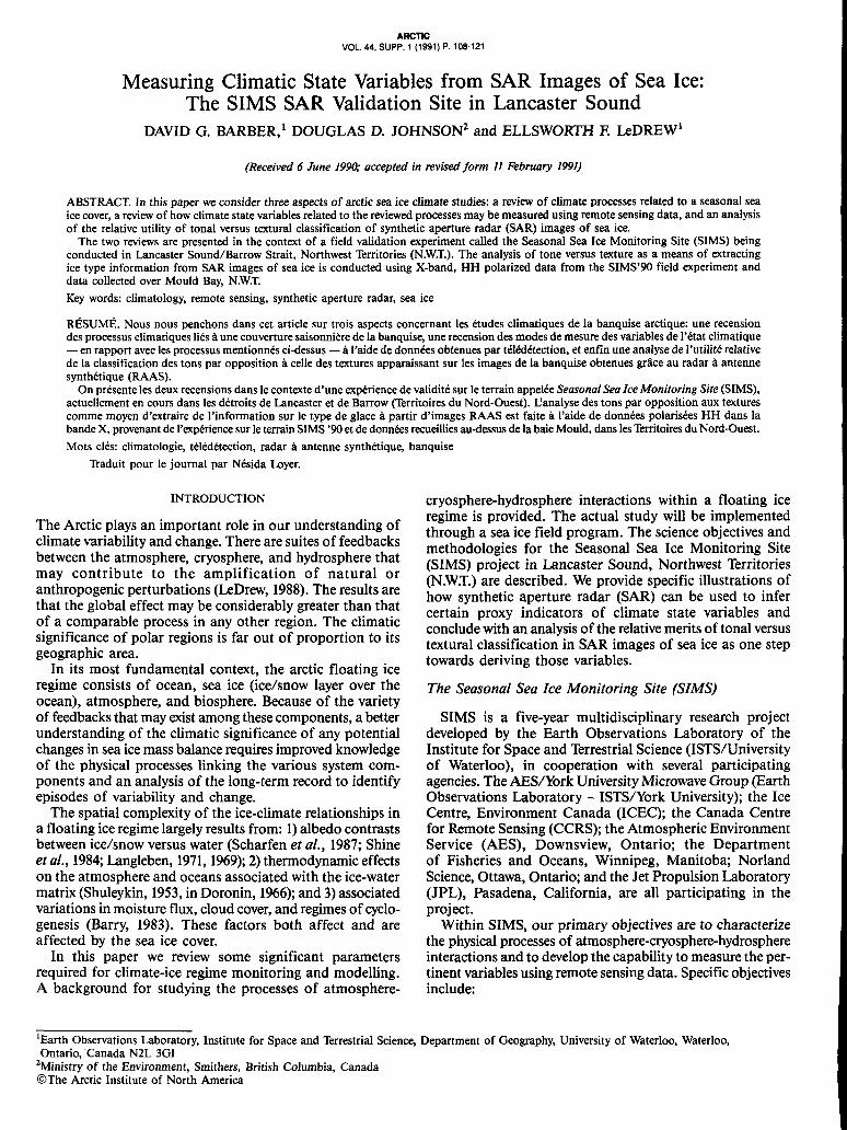
surface validation site in Lancaster Sound, N.W.T. (Fig. 1). The pilot field study was conducted from 12 May to 7 June 1990. The 1990 field program was held coincident with over- flights from a SAR aircraft (the X-band ICEC Challenger SAR, contracted from Intera Technologies). Four orbital sensors provided data in the visible, near infrared, thermal infrared, and microwavelengths (Landsat TM [Thematic Mapper]; SPOT [SystCme pour d’observation de la terre]; the U.S.-National Oceanic and Atmospheric Administration

AVHRR [Advanced Very High Resolution Radiometer]; and the SSMA [Special Sensor for Microwave/Imaging]). Starting in 1991, new orbital systems will become available through such programs as Europe’s ERS-1 and Canada’s Radarsat. Both of these satellites will carry synthetic aperture radars (SARs), which are capable of “all weather” and “day-night” mapping of the earth’s surface. A suite of sensors from the U.S. National Aeronautics and Space Administration’s proposed Mission to Planet Earth is also expected to provide remote sensing data appropriate for this field program in future years.

Remote Sensing of Physical Processes A considerable amount of energy has been expended in

developing methodologies by which remote sensing data can be utilized to improve our understanding of the physical processes occurring across the atmosphere-cryosphere- hydrosphere interface. Major projects such as AIDJEX (Arctic Ice Dynamics Joint Experiment), BESEX (Bering Sea Experiment), LIMEX (Labrador Ice Margin Experiment), MIZEX (Marginal Ice Zone Experiment), and NORSEX (Norwegian Remote Sensing Experiments) have added considerably to our understanding of physical processes inherent in the atmosphere-cryosphere-hydrosphere system. These projects have also been particularly useful in developing remote sensing methodologies that can be utilized to parameterize the important variables for subsequent

FIG. I . Field validation site for the Lancaster Sound SIMS project. Intensive and extensive sample areas are for the 1990 field season.

110 / D.G. BARBER et al.

modelling and monitoring research. The SIMS project is intended to build on these past achievements and to develop methodologies by which remote sensing data can be used to measure climate state variables.

Although neither inclusive nor exhaustive, the cryospheric processes and associated variables most suited to remote measurement include thermodynamic properties of sea ice, albedo; latent heat of sea ice, atmospheric drag coefficients, sea ice - cloud interactions, and snow cover. In what follows we explicitly define each of these processes/variables, thereby defining the critical physical components of the SIMS program.

Thermodynamic Properties of Sea Ice: The presence of sea ice restricts exchanges of heat (see Badgley, 1966; Gud- mandsen, 1985; Maykut, 1978, 1982; Zwally et al., 1983), mass, momentum, and chemical constituents between the ocean and the atmosphere. The thermal insulation of the i cehow layers is a function of the temperature gradient, density, salinity, and specific heat of the layer@) (Maykut and Untersteiner, 1982).

Breaks in the sea ice insulating layer (polynyas, leads, cracks) create areas of enhanced turbulent heat flux, thereby contributing to the enthalpy of the overlaying air mass. These areas account for only a small portion of the surface area of the Arctic, yet may contribute significantly to the total turbulent heat fluxes (Maykut, 1982). Seasonal or interannual changes in ice extent and/or ice type may have substantial energy budget implications (Carleton, 1981). Due to differing heat exchanges between atmosphere-ice or atmosphere-open water regimes, it may be expected that variations in the distribution of ice/water surfaces will affect diabatic heating and regional synoptic activity within the atmosphere. Thus, when the ocean-ice-atmosphere system is considered as a whole, the most significant influence on atmosphere-surface interactions is the relative distribution of ice/water surfaces (Crane, 1981).

Remote sensing at thermal infrared wavelengths (- 8.0-11.0 pm) can provide information on the surface temperature of sea ice (Steffen and Lewis, 1988) and can be used to monitor snow surface temperature throughout the snowmelt period (Barnes, 1981, in Foster et al., 1987) - a period important in energy balance studies (Foster et al., 1987). Thermal imagery is also commonly used for small-scale studies of ice extent and ice movement and can be used for a relative assessment of ice thickness (up to about 1 m) (Barnes et al., 1974; Dey, 1980; Poulin, 1975; Weeks, 1981). For example, Ito (1985) used Landsat MSS 7 (near-infrared) data to observe sea ice distribution and decay in the North Water during 1973. Thermal infrared data have not been used extensively in the calculation of radiative and sensible heat fluxes (Carsey and Zwally, 1986).

SAR can be used to parameterize information on ice thickness as a function of general ice type (Le., new, first- year, and multiyear ice). The all-weather day-night sensing capabilities of this active microwave sensor make it ideal for arctic applications. Upcoming orbital SARs (ERS-1, JERS-1, and Radarsat) will provide spatial samples of ice conditions (at from 20 to 500 km swaths in its SCANSAR operational mode) at a temporal resolution of daily to weekly for various parts of the Canadian Arctic.

Albedo: The typical integrated albedo of a snow surface is on the order of 0.85, for water it is 0.05-0.10, and for ice surfaces 0.6 (water free) to 0.2 (water covered) (Barry, 1983).

Albedo also changes as a function of ice type. The large water/ice albedo contrast exerts a strong control on regional radiation and energy balances. Inherent in a change of such surface covers is a positive feedback (Crane, 1981; Dickinson et al., 1987; Hansen et al., 1984; Hartmann, 1984; Kellogg, 1983; Schneider and Dickinson, 1976; Robock, 1983). Large changes in surface albedo occur during the melt period of the ice snowpack (Langleben, 1971), which also has significant implications regarding the ice regime energy balance. The study of such melt events and associated snowmelt-related albedo changes could provide an index of interannual climate variability; subsequent understanding of these variations could then be applied to climate models, resulting in a more representative knowledge of arctic spring transition conditions (Anderson, 1987a).

It should be possible to develop proxy indicators of albedo using surface structure information (from SAR) and/or thermal wavelength imagery complementing the melt-event work already done with passive microwave data (e.g., Garrity et al., 1990; Crane and Anderson, 1988; Crane, 1989), and visible data (e.g., Robinson et al., 1986, 1987). Preliminary analysis of the application of SAR imagery to development of these proxy indicators was conducted during the Labrador Ice Margin Experiment (LIMEX’89). Results indicate that a relationship exists between surface albedo and ice type. Five types of ice were considered during the LIMEX project: first- year ice, black/grey nilas, grease ice, open water, and frozen brash. During the SIMS’90 field experiment surface reflectances were coupled with geophysical measurements of the snow cover so that optical extinction properties could be linked with the dielectric scattering properties of the melting snow cover. A thorough comparative analysis of the physics of these electromagnetic interactions is forthcoming from the authors.

Latent Heat of Sea Ice: Sea ice acts as an energy sink when it is transported to lower latitudes via a negative latent heat export. This also serves to reduce regional heat contrasts in sea ice-covered regions (Parkinson et al., 1987). Thus, polar regions serve as a major heat sink in the small-scale atmospheric and oceanic circulations of the earth (Gud- mandsen, 1985).

The optimal remote sensing method for mapping the concentration and distribution of this latent heat source is passive microwave data. Data on percentage of ice cover, a general indication of ice type, and an indication of oceanic circulation patterns can be determined for grid point data on a regional or hemispheric scale. These data are available on a routine basis and provide excellent macro coverage of the Canadian Arctic.

Atmospheric Drag Coefficient: Estimates of the atmospheric drag over sea ice are useful in studying interactions among the ocean, ice, and atmosphere and in modelling ice motion or atmospheric forcing. Winds, and their associated effect on ice motion, have a strong control on sea ice mass balance. Ice divergence or convergence can alter energy exchanges across the atmosphere-cryosphere- hydrosphere interface and can result in accelerated ice for- mation or ice ablation, depending on the time of year (Gud- mandsen, 1985) and region. In addition, wind-induced ice floe motion creates a surface stress gradient that modifies the ocean mixed layer. This is a common cause for the upwelling observed at ice margins (Carsey and Zwally, 1986; Gudmandsen, 1985). These upwelling areas bring nutrient-

rich deep water to the euphotic zone, where photosynthetic processes make use of organic carbon in the production of phytoplankton. Proliferation at this level of the food chain stimulates production at all other levels, making these areas biologically important. Where ice motion is inhibited, a sea ice cover can act to reduce wind/wave surface stress, which, in turn, dampens surface turbulent exchange with the atmosphere (OIES, 1988).

It has been proposed (Burns, 1990) that since SAR is sensitive to microscale surface roughness (particularly during the winter season), there may be a relationship between the atmospheric drag over the ice surface and roughness of that surface measured by a synthetic aperture radar (SAR). Anderson (1987b) summarized various observations of the relationship between floe size, concentration, and ice roughness with atmospheric drag. Anderson found that for a neutral atmospheric stratification the coefficient of drag (Cd) increases as the ice concentration increases and that, if concentration is held constant, Cd is a function of flow size and ice roughness.

Burns (1990) found that in areas of relatively smooth pack ice the backscattering information contained within SAR was at a scale inappropriate to infer the atmospheric drag coefficient. The presence of ridges in pack ice and the sensitivity of SAR to the frequency and height of ridges are presented as areas requiring future research. However, Burns (1990) did find that SAR provided good estimates of Cd within a marginal ice zone (MIZ).

Sea Ice-Cloud Interactions: Very little information is available regarding cloud cover and sea ice extent, although there have been correlations between ice extent and cloudiness (Crane and Barry, 1984). The problem is a difficult one due to the compensatory effects clouds have on the shortwave and longwave radiation balances; relative domination of either flux is sensitive to the season and the nature of the underlying sea ice surface (Shine and Crane, 1984) and cloud character. Maltese et al. (1984) found that the simultaneous presence of ice-albedo and cloud amount-temperature feedbacks greatly amplifies the magnitude of a climatic response to an extreme forcing. Barry et al. (1984), Crane and Barry (1984), Shine et al. (1984), Shine and Crane (1984), and Shine and Henderson-Sellers (1984) provide detailed insights into this issue.

The spectral albedo and thermal fluxes are altered by changing cloud cover, the former by decreasing incident shortwave radiation at the surface and the latter by reradiation to the surface from the warmer cloud surface. Herman (1980) reports values for net longwave radiation at the surface of -60 W m-', in contrast to -32 W m-' for cloud-free versus cloud-covered conditions in January for a test area in the central Arctic (Barry, 1983).

Generalizations about the radiation balance over the ice surface can be inferred by determining relationships between shortwave and longwave components associated with different ice surfaces in overcast conditions. Surface structure from SAR and cloud height and optical thickness from thermal infrared and optical sensors may be synergistically useful.

Snow Cover: Sea ice snow cover is important due to its thermodynamic effects (Carsey, 1984) and its control on surface albedo (Scharfen et al., 1987). The timing of snowmelt initiation varies, causing significant impacts on the Arctic Basin heat and mass balance (due to the strong control exerted

ARCTIC SEA ICE CLIMATE STUDIES / 111

by surface albedo), which could ultimately affect the long- term stability of the ice (Fletcher, 1966; Barry, 1985, in Robinson et al., 1987). SAR signatures of sea ice are also strongly controlled by the onset of melt. The dielectric constant of the snow/ice matrix changes dramatically as the amount of free water increases. This causes a shift in the backscattering characteristics as recorded by the SAR (Livingstone et al., 1987).

Snow cover is essentially transparent in the winter season at microwavelengths (Garrity et al., 1990; Kim et al., 1985) at all naturally occurring ice roughness scales except the very smooth (Bredow and Gogennini, 1990). In the spring, snow cover provides the most interesting changes in radar backscatter when free water becomes available in the snow pack. As the water content increases, the penetration depth of microwaves into the pack decreases (Drinkwater, 1989). As the penetration depth decreases, the average scattering from a snow-covered ice surface contains an increasing contribution from the snow volume and snow surface geometry. Volume scattering within the snow pack arises from the metamorphosis of snow crystals into polycrystalline aggregates and the sublimation of water vapour into ice lenses and layers. The relative contribution of snow surface roughness to the backscattering of microwave energy increases as the free water content of the snow increases. It has also been suggested that during the fall season the high saline snow cover, created by the destructive metamorphosis of frost flowers, has a strong influence on the backscatter recorded by the SAR imaging system (Drinkwater and Crocker, 1988).

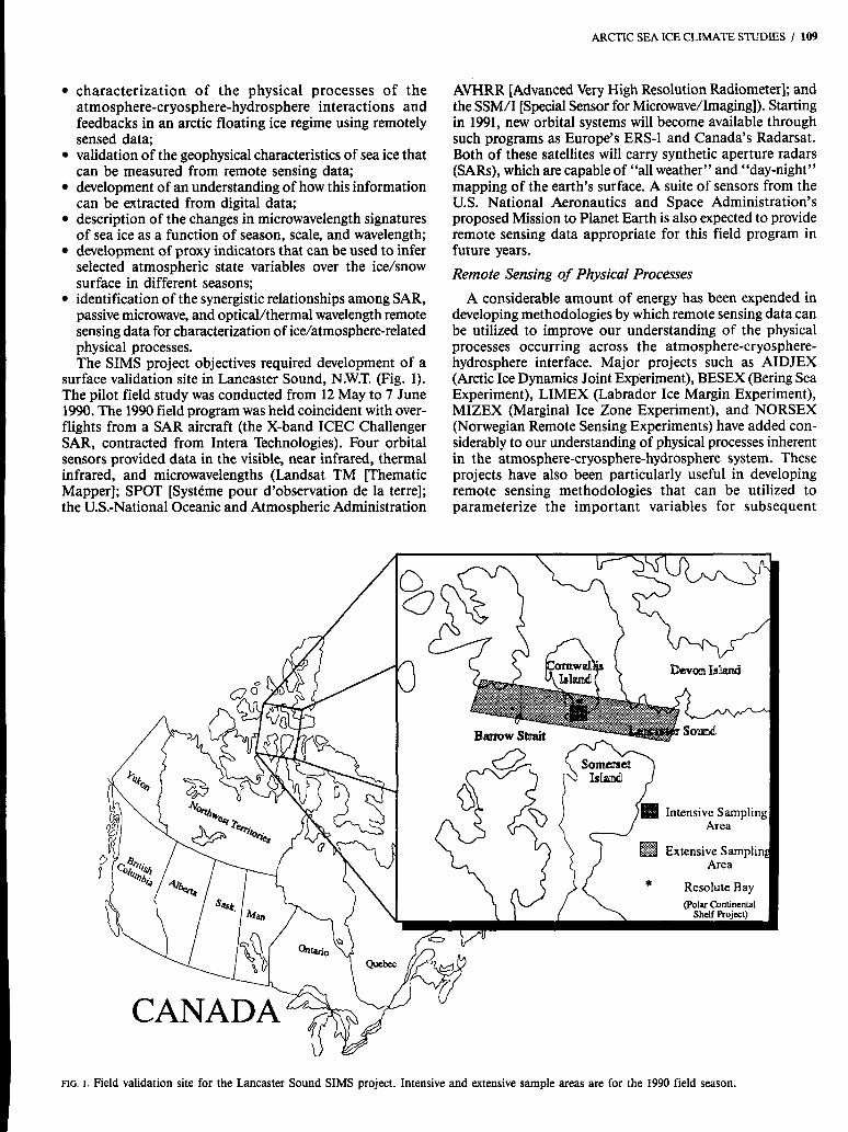
Remote Measurement: It will require a wide variety of instruments to make the measurements required to develop an understanding of the physical processes active in the floating ice regime. Variables marked with an asterisk (*) in Bble 1 can be measured, to varying extents, with SAR. Integrated with surface pressure, temperature, humidity, and net radiation, these variables are essential parameters in modeling atmosphere-cryosphere-hydrosphere climate interactions (Gudmandsen, 1985).

TABLE 1. Sea ice and related parameters of importance in different operational and research areas'

Area of interest Sea ice and related parameters Albedo* Extent, type, surface cover: melt pond

Ocean/ice/atmosphere Lead area; thin ice vs. thick ice, snow thermodynamics* vs. no snow cover, air temperature,

Latent heat export Thickness, drift velocity Surface stress* Drift velocity, top and bottom ice

Sub-ice primary production* Ice type, snow cover Ocean mixed layer* Ice growth and ablation rates, drift

coverage, melt initiation

wind velocity, ice concentration

roughness, wind velocity, current velocity

velocity, current velocity, ice cover, water column stability, water temperature and salinity, wind velocity, depth*

*In addition to surface pressure, temperature, humidity, and net radiation, those variables marked "*" denote parameters essential in modeling of

'Adapted from Carsey and Hoit (1987), Crane (1981), Gudmandsen (198% atmosphere-cryosphere-hydrosphere climate interactions.

Welch and Bergmann (1989), Thomas (1986), Weaver et al. (1987), and Weeks (1981).

112 1 D.G. BARBER et al.

ANALYSIS OF SAR SEA ICE IMAGES

Background

Microwave energy is transmitted from a synthetic aperture radar to the ice surface where the radiation interacts with the surface material and is backscattered to the sensor. The probabilities associated with a particular magnitude of backscatter (a”) are a function of the dielectric properties of the surface, the roughness of the surface relative to the wavelength, and SAR system parameters (i.e., polarization, incidence angle, and frequency). Although seasonality has a large impact on both the dielectric properties of sea ice and the surface roughness of the ice, and therefore 8, a winter sea ice scene is largely dominated by surface scattering from young ice forms and volume scattering from the bubble matrix in the upper layer of multiyear ice forms (Kim et al., 1985; Ulaby et al., 1986). Surface scattering of a homogeneous i cehow surface consists of a continuum between specular reflection (new ice forms and calm open water) to diffuse reflection where roughness (h) can be defined by the Rayleigh criterion (1); where X is the SAR wavelength:

X h < - 8 cos 8 (1)

(If h is true, then the surface is considered smooth.) System parameters such as frequency, polarization, and

incidence angle also play an important role in the amount of backscattered radiation received by the SAR antenna and on the spatial arrangements of the grey levels (i.e., texture) in the SAR scene. Modelling studies have provided valuable information on the optimal radar parameters for sea ice. Although a detailed account is beyond the scope of this paper, excellent reviews are available on the relative merits of system parameters (e.g., Kim et al., 1985), seasonality (e.g., Livingstone et al., 1987), and the contribution of different sea ice geophysical parameters (e.g., Ulaby et al., 1986) to backscatter from sea ice.

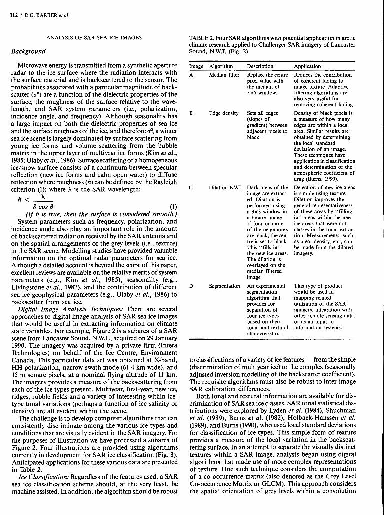
Digital Image Analysis Techniques: There are several approaches to digital image analysis of SAR sea ice images that would be useful in extracting information on climate state variables. For example, Figure 2 is a subarea of a SAR scene from Lancaster Sound, N.W.T., acquired on 29 January 1990. The imagery was acquired by a private firm (Intera Technologies) on behalf of the Ice Centre, Environment Canada. This particular data set was obtained at X-band, HH polarization, narrow swath mode (61.4 km wide), and 15 m square pixels, at a nominal flying altitude of 11 km. The imagery provides a measure of the backscattering from each of the ice types present. Multiyear, first-year, new ice, ridges, rubble fields and a variety of interesting within-ice- type tonal variations (perhaps a function of ice salinity or density) are all evident within the scene.

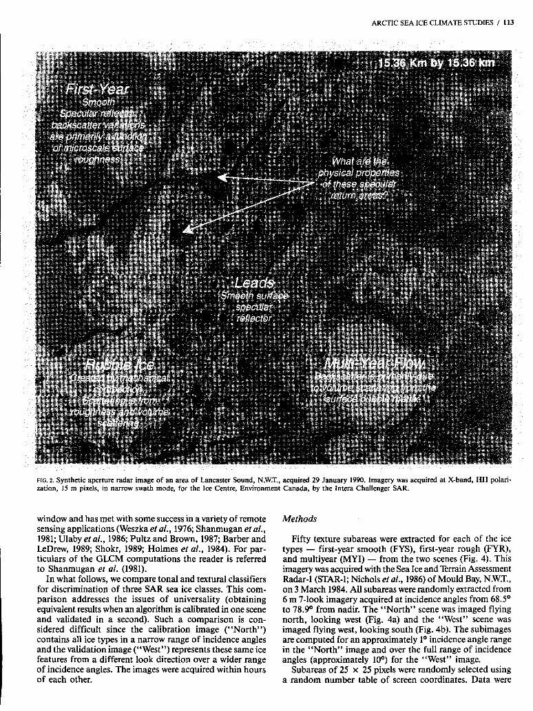
The challenge is to develop computer algorithms that can consistently discriminate among the various ice types and conditions that are visually evident in the SAR imagery. For the purposes of illustration we have processed a subarea of Figure 2. Four illustrations are provided using algorithms currently in development for SAR ice classification (Fig. 3). Anticipated applications for these various data are presented in Table 2.

Ice Classification: Regardless of the features used, a SAR sea ice classification scheme should, at the very least, be machine assisted. In addition, the algorithm should be robust

TABLE 2. Four SAR algorithms with potential application in arctic climate research applied to Challenger SAR imagery of Lancaster Sound, N.W.T. (Fig. 2)

Image Algorithm Description Application Reduces the contribution A Median filter Replace the centre

pixel value with the median of 5x 5 window.

B Edge density Sets all edges (slopes of gradient) between adjacent pixels to black.

C Dilation-NWI Dark areas of the image are extracted. Dilation is performed using a 3x3 window in a binary image. If four or more of the neighbours are black, the centre is set to black. This “fills in” the new ice areas. The dilation is overlayed on the median filtered image.

segmentation algorithm that provides for separation of four ice types based on their tonal and textural characteristics.

D Segmentation An experimental

of coherent fading to image texture. Adaptive filtering algorithms are also very useful for removing coherent fading. Density of black pixels is a measure of how many edges are within a local area. Similar results are obtained by determining the local standard deviation of an image. These techniques have application in classification and determination of the atmospheric coefficient of drag (Burns, 1990).

Detection of new ice areas is simple using texture. Dilation improves the general representativeness of these areas by “filling in” areas within the new ice areas that were not classes in the tonal extraction. Measurements, such as area, density, etc., can be made from the dilated imagery.

This type of product would be used in mapping related utilization of the SAR imagery, integration with other remote sensing data, or as an input to information systems.

to classifications of a variety of ice features - from the simple (discrimination of multiyear ice) to the complex (seasonally adjusted inversion modelling of the backscatter coefficient). The requisite algorithms must also be robust to inter-image SAR calibration differences.

Both tonal and textural information are available for discrimination of SAR sea ice classes. SAR tonal statistical distributions were explored by Lyden et al. (1984), Shuchman et al. (1989), Burns et al. (1982), Holbaek-Hanssen et al. (1989), and Burns (1990), who used local standard deviations for classification of ice types. This simple form of texture provides a measure of the local variation in the backscattering surface. In an attempt to separate the visually distinct textures within a SAR image, analysts began using digital algorithms that made use of more complex representations of texture. One such technique considers the computation of a co-occurrence matrix (also denoted as the Grey Level Co-occurrence Matrix or GLCM). This approach considers the spatial orientation of grey levels within a convolution


FIG. 2. Synthetic aperture radar image of an area of Lancaster Sound, N.W.T., acquired 29 January 1990. Imagery was acquired at X-band, HH polarization, 15 m pixels, in narrow swath mode, for the Ice Centre, Environment Canada, by the Intera Challenger SAR.

window and has met with some success in a variety of remote sensing applications (Weszka et al., 1976; Shanmugan et al., 1981; Ulaby et al., 1986; Pultz and Brown, 1987; Barber and LeDrew, 1989; Shokr, 1989; Holmes et al., 1984). For particulars of the GLCM computations the reader is referred to Shanmugan et al. (1981).

In what follows, we compare tonal and textural classifiers for discrimination of three SAR sea ice classes. This comparison addresses the issues of universality (obtaining equivalent results when an algorithm is calibrated in one scene and validated in a second). Such a comparison is considered difficult since the calibration image (“North”) contains all ice types in a narrow range of incidence angles and the validation image (“West”) represents these same ice features from a different look direction over a wider range of incidence angles. The images were acquired within hours of each other.

Methods

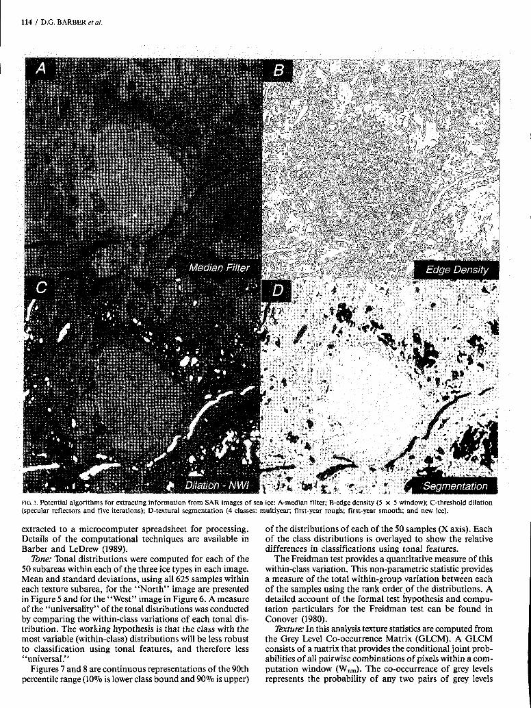
Fifty texture subareas were extracted for each of the ice types - first-year smooth (FYS), first-year rough (FYR), and multiyear (MYI) - from the two scenes (Fig. 4). This imagery was acquired with the Sea Ice and Terrain Assessment Radar-1 (STAR-1; Nichols et al., 1986) of Mould Bay, N.W.T., on 3 March 1984. All subareas were randomly extracted from 6 m 7-look imagery acquired at incidence angles from 68.5’ to 78.90 from nadir. The “North” scene was imaged flying north, looking west (Fig. 4a) and the “West” scene was imaged flying west, looking south (Fig. 4b). The subimages are computed for an approximately 1’ incidence angle range in the “North” image and over the full range of incidence angles (approximately 10’) for the “West” image.

Subareas of 25 x 25 pixels were randomly selected using a random number table of screen coordinates. Data were


FIG. 3. Potential algorithms for extracting information from SAR images of sea ice: A-median filter; B-edge density (5 x 5 window); C-threshold dilation (specular reflectors and five iterations); D-textural segmentation (4 classes: multiyear; first-year rough; first-year smooth; and new ice).

extracted to a microcomputer spreadsheet for processing. of the distributions of each of the 50 samples (X axis). Each Details of the computational techniques are available in of the class distributions is overlayed to show the relative Barber and LeDrew (1989). differences in classifications using tonal features.

Tone: Tonal distributions were computed for each of the The Freidman test provides a quantitative measure of this 50 subareas within each of the three ice types in each image. within-class variation. This non-parametric statistic provides Mean and standard deviations, using all 625 samples within a measure of the total within-group variation between each each texture subarea, for the “North” image are presented of the samples using the rank order.of the distributions. A in Figure 5 and for the “West” image in Figure 6. A measure detailed account of the formal test hypothesis and compu- of the “universality” of the tonal distributions was conducted tation particulars for the Freidman test can be found in by comparing the within-class variations of each tonal dis- Conover (1980). tribution. The working hypothesis is that the class with the Texture: In this analysis texture statistics are computed from most variable (within-class) distributions will be less robust the Grey Level Co-occurrence Matrix (GLCM). A GLCM to classification using tonal features, and therefore less consists of a matrix that provides the conditional joint prob- “universal.’’ abilities of all pairwise combinations of pixels within a com-

Figures 7 and 8 are continuous representations of the 90th putation window (Wn,,,). The co-occurrence of grey levels percentile range (10% is lower class bound and 90% is upper) represents the probability of any two pairs of grey levels

FIG. 4. STAR-1 SAR images of Mould Bay, 3 March 1984. “North” (a) image and “West” (b) image, showing the flight orientations, incidence angles, and orientation of the parameters used in computing the grey level Co-ocurrence matrices (GEMS).

occurring, conditional on the interpixel sampling distance (6) and orientation (a) used for computation. Algebraically Uniformity this can be expressed as (2), where Cij is defined in (3), following Haralick et al. (1973):

i = l j = 1

Pr(x)= [Cij I 6,a] Correlation

Entropy ij = 1 i = l j = l

where P is the frequency of occurrence of grey levels i and j. Summation over n refers to the total number of pixel pairs, Dissimilarity f: f:cIJ I(i - j)l (7)

which is dependent on the parameter 6 and the subscripts n and m from W,,,,,. In the following analysis an 8-bit image has been quantized to 4 to reduce computation time (SAR Contrast imagery is usually 8 bit or 256 grey levels; 4 bit results in zcIJ (i - j)2 (8) 16 grey levels, thereby reducing computation time). Texture i = l j = 1

statistics are computed from the matrix and represent a single spatial measure of the image texture from which the GLCM SDC is computed. Seven commonly used texture statistics (Barber 2 ( p y and LeDrew, 1989; Conners et al., 1984; Pultz and Brown, , = I

n

i = l j = l

n

1987; Shanmugan et al., 1981) are used: j = l (9)

116 I D.G. BARBER er al.

where: Cij is the matrix cell frequencies normalized by the number of pixel pairs Pij. n is the number of pixel pairs in the image at CY,^). ax is the sample standard deviation of row i. uy is the sample standard deviation of column j. px is the sample mean of row i. py is the sample mean of column j. For further details of the computation see Barber and LeDrew (1989) or Shanmugan et al. (1981).

A measure of the “universality” of the textural distributions was conducted by comparing the classification accuracies of a set of texture statistics computed in one image (“North” [Fig. 4a], calibration set) and directly applying the algorithm to the second (“West” [Fig. 4b], validation set).

Multiple Discriminant Analysis (MDA) was computed using a Macintosh II microcomputer, based on algorithms described in Ludwig and Reynolds (1988) and using SYSTAT (Wilkinson, 1987). MDA is a statistical technique that can be used to define spatial patterns and to assist in meaningful interpretation of these patterns (Williams and Titus, 1983). We used MDA as a means of determining which set of p variables maximize discrimination of k ice classes. Identifi- cation of classes is done a priori, either through functional description of classes (as we have done) or through some form of ordination. The number of discriminant functions that result is the smaller of k-1 or p . MDA finds a set of linear transformations that maximizes the inter- to intra-class variation over k. This is equivalent to maximizing the F ratio of a one-way analysis of variance (Manly, 1986). The first

x5 x10 x15 X20 x25 %O %5 %O %5 x50

Sample Number

r n c s Scatter diagram of mean tone vs. standard deviation of tone for 150 samples of 625 pixels from three ice types in the “North” (Fig. 4a) image.

x5 x10 x15 x20 x25 %O %5 %O x45 x50

Sample Number

FIG. 6. Scatter diagram of mean tone vs. standard deviation of tone for 150 samples of 625 pixels from three ice types in the “West” (Fig. 4b) image.

function (Zl) maximizes the inter- versus intra-class variation over the entire data matrix. The second function (ZZ) maximizes the F ratio, with the important limitation that ZZ is statistically orthogonal to Z1, and so on (Manly, 1986). In our analysis p is 2 or 3 variables and k is 3 ice classes.

Computation of the calibration set discriminant functions was based on 50 samples from each ice type. The resulting discriminant functions were then applied to the validation set. All texture statistics in this analysis were computed at interpixel sampling distances of one (6=1) and orientations of zero @=O). This orientation is parallel to the look direction in both “North” and “West” images (Fig. 4a,b).

Contingency tables were tabulated for classification accuracies of the validation and calibration data sets. A Kappa Coefficient (K) and variance (K,) of this statistic (Bishop et al., 1975) were computed for both the calibration (Kc) and validation (KY) sets based on algorithms developed by Barber (1989). Confidence intervals were computed based on an assumed normal distribution of the K-hat statistic at a 90% level against a Q p e I error (“Significant Difference’’ in Tables 5 and 6).

Results

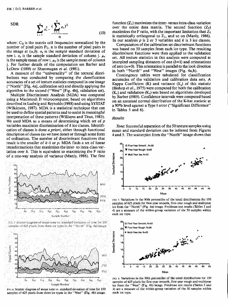
Tone: Successful separation of the 50 texture samples using mean and standard deviation can be inferred from Figures 4 and 5 . The scatterplot from the “North” image shows that

O Firsl-Year Smooth ; N=50

‘I Firsl-Year Rwgh N-50

I O 5 10 15 20 25 30 35 40 45 50 55 60 65

M W

FIG. 7. Variations in the 90th percentiles of the tonal distributions for 150 samples of 625 pixels for first-year smooth, first-year rough and multiyear ice from the “North” (Fig. 4a) image. Freidman test results (lkbles 3 and 4) are a measure of the within-group variation of the 50 samples within each ice type.

O First-Year Smooth; N-50

‘I First-Year Rough: N-50

6 + MuIli-Year ka; N=5O +

. . . . . . . . . . . . . . . . . . . . . . . . . . . O 5 10 15 20 25 30 35 40 45 50 55 60 65

M W

FIG. S. Variations in the 90th percentiles of the tonal distributions for 150 samples of 625 pixels for first-year smooth, first-year rough and multiyear ice from the “West” (Fig. 4b) image. Freidman test results (’kbles 3 and 4) are a measure of the within-group variation of the 50 samples within each ice type.

mean tone is less variable (lower spread of values along the X axis in Figure 5 as opposed to Figure 6) in the image with the smaller incidence angle. The range of standard deviations is nearly identical in the “North” and “West” images.

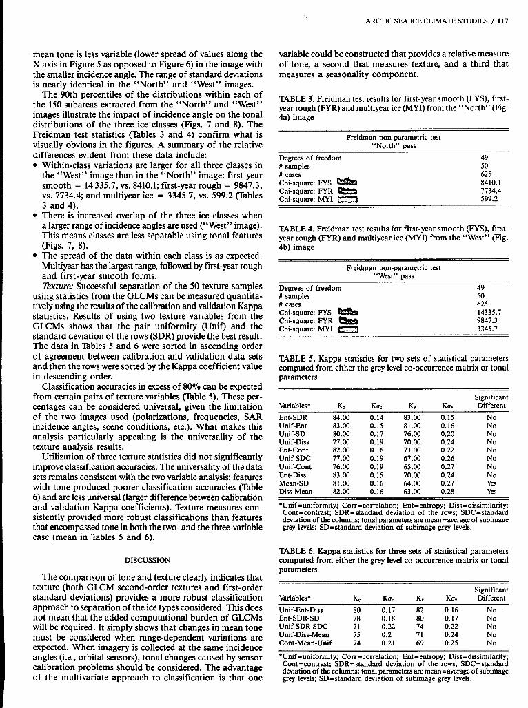
The 90th percentiles of the distributions within each of the 150 subareas extracted from the “North” and “West” images illustrate the impact of incidence angle on the tonal distributions of the three ice classes (Figs. 7 and 8). The Freidman test statistics (’Thbles 3 and 4) confirm what is visually obvious in the figures. A summary of the relative differences evident from these data include:

Within-class variations are larger for all three classes in the “West” image than in the “North” image: first-year smooth = 14 335.7, vs. 8410.1; first-year rough = 9847.3, vs. 7734.4; and multiyear ice = 3345.7, vs. 599.2 (’kbles 3 and 4). There is increased overlap of the three ice classes when a larger range of incidence angles are used (“West” image). This means classes are less separable using tonal features (Figs. 7, 8). The spread of the data within each class is as expected. Multiyear has the largest range, followed by first-year rough and first-year smooth forms. Texture: Successful separation of the 50 texture samples

using statistics from the GLCMs can be measured quantita- tively using the results of the calibration and validation Kappa statistics. Results of using two texture variables from the GLCMs shows that the pair uniformity (Unif) and the standard deviation of the rows (SDR) provide the best result. The data in ’Thbles 5 and 6 were sorted in ascending order of agreement between calibration and validation data sets and then the rows were sorted by the Kappa coefficient value in descending order.

Classification accuracies in excess of 80% can be expected from certain pairs of texture variables (’kble 5) . These per- centages can be considered universal, given the limitation of the two images used (polarizations, frequencies, SAR incidence angles, scene conditions, etc.). What makes this analysis particularly appealing is the universality of the texture analysis results.

Utilization of three texture statistics did not significantly improve classification accuracies. The universality of the data sets remains consistent with the two variable analysis; features with tone produced poorer classification accuracies (’kble 6) and are less universal (larger difference between calibration and validation Kappa coefficients). k t u r e measures consistently provided more robust classifications than features that encompassed tone in both the two- and the three-variable case (mean in ’kbles 5 and 6).

DISCUSSION

The comparison of tone and texture clearly indicates that texture (both GLCM second-order textures and first-order standard deviations) provides a more robust classification approach to separation of the ice types considered. This does not mean that the added computational burden of GLCMs will be required. It simply shows that changes in mean tone must be considered when range-dependent variations are expected. When imagery is collected at the same incidence angles (i.e., orbital sensors), tonal changes caused by sensor calibration problems should be considered. The advantage of the multivariate approach to classification is that one


variable could be constructed that provides a relative measure of tone, a second that measures texture, and a third that measures a seasonality component.

TABLE 3. Freidman test results for first-year smooth (FYS), first- year rough (FYR) and multiyear ice (MYI) from the “North” (Fig. 4a) image

Freidman non-parmetric test “North” pass

Degrees of freedom 49 # samples 50 # cases 625 Chi-square: FYS && 8410.1 Chi-square: FYR 7734.4 Chi-square: MY1 599.2

TABLE 4. Freidman test results for first-year smooth (FYS), first- year rough (FYR) and multiyear ice (MYI) from the “West” (Fig. 4b) image

Freidman non-parametric test “West” pass

Degrees of freedom 49 # samples 50 # cases 625 Chi-square: FYS 14335.7 Chi-square: FYR 9847.3 Chi-square: MY1 3345.7

TABLE 5 . Kappa statistics for two sets of statistical parameters computed from either the grey level co-occurrence matrix or tonal parameters

Significant Variables* KC Kuc K” Different Ent-SDR Unif-Ent Unif-SD Unif-Diss Ent-Cont Unif-SDC Unif-Cont Ent-Diss Mean-SD Diss-Mean

84.00 0.14 83.00 0.15 83.00 0.15 81.00 0.16 80.00 0.17 76.00 0.20 77.00 0.19 70.00 0.24 82.00 0.16 73.00 0.22 77.00 0.19 67.00 0.26 76.00 0.19 65.00 0.27 83.00 0.15 70.00 0.24 81.00 0.16 64.00 0.27 82.00 0.16 63.00 0.28

No No No No No No No No Yes Yes

*Unif=uniformity; Corr=correlation; Ent=entropy; Diss=dissimilarity; Cont=contrast; SDR=standard deviation of the rows; SDC=standard deviation of the columns; tonal parameters are mean=average of subimage grey levels; SD=standard deviation of subimage grey levels.

TABLE 6. Kappa statistics for three sets of statistical parameters computed from either the grey level co-occurrence matrix or tonal parameters

Significant Variables* K, Kuc K, Ku, Different Unif-Ent-Diss 80 0.17 82 0.16 No Ent-SDR-SD 78 0.18 80 0.17 No Unif-SDR-SDC 71 0.22 74 0.22 No Unif-Diss-Mean 75 0.2 71 0.24 No Cont-Mean-Unif 74 0.21 69 0.25 No

*Unif=uniformity; Corr=correlation; Ent=entropy; Diss=dissimilarity;

deviation of the columns; tonal parameters are mean=average of subimage Cont-contrast; SDREstandard deviation of the rows; SDC-standard

grey levels; SD=standard deviation of subimage grey levels.


Our primary objective in this paper has been to describe how SAR data can be used to infer properties of the ice surface and how this surface structure information could be used in climatological analysis. The large data volumes forthcoming from the orbital SAR sensors makes digital interpretation (and therefore development of appropriate computer algorithms) a necessity. Since we generally have no apriori knowledge of the scene, we must validate the backscattering characteristics of SAR imagery within the range of conditions we know create changes in backscatter signatures and determine the stability of these relationships.

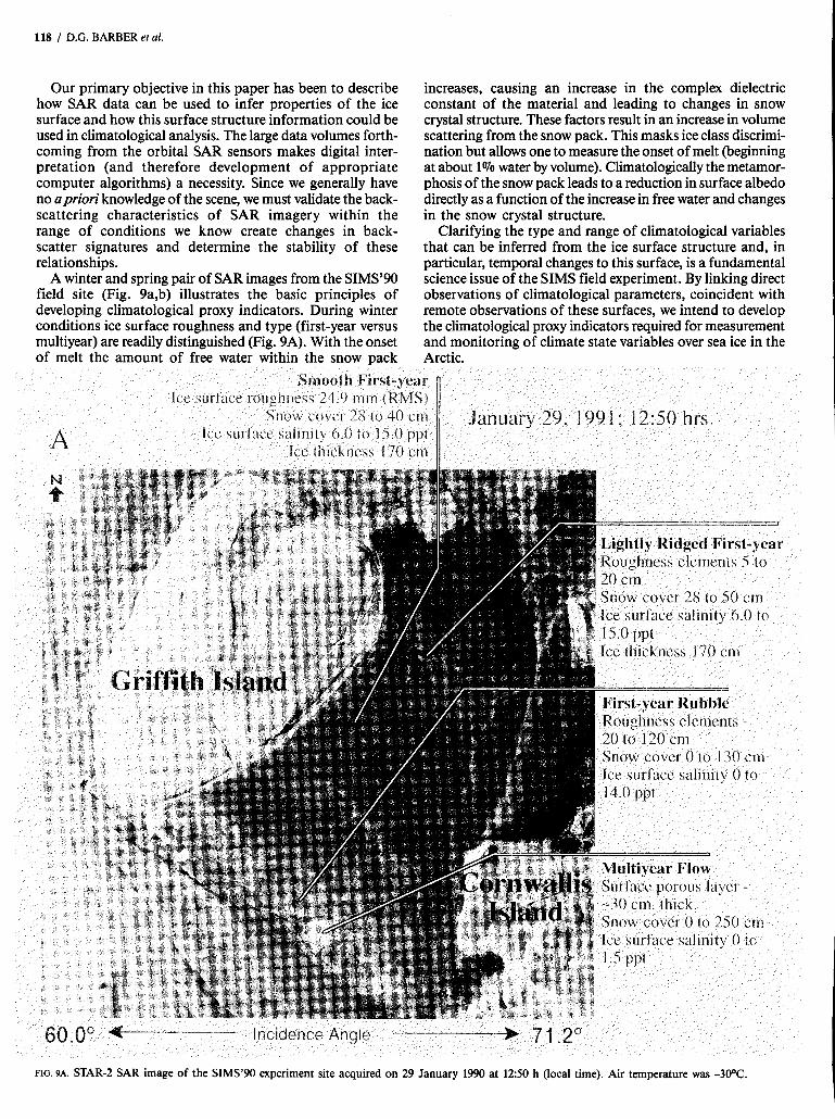
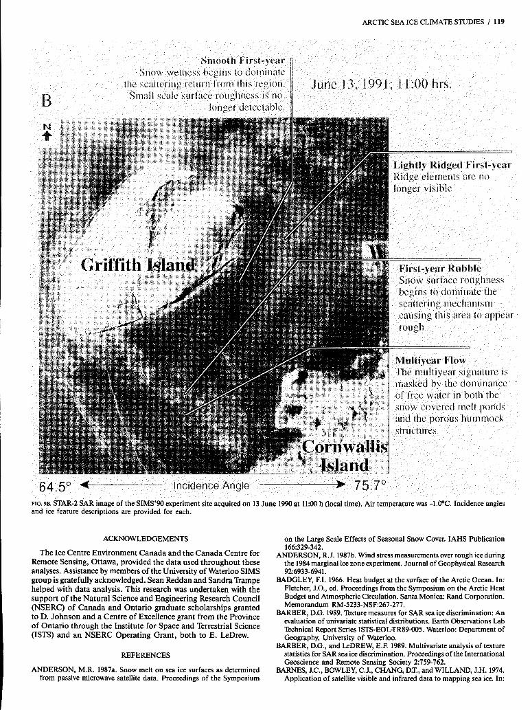
A winter and spring pair of S A R images from the SIMS’90 field site (Fig. 9a,b) illustrates the basic principles of developing climatological proxy indicators. During winter conditions ice surface roughness and type (first-year versus multiyear) are readily distinguished (Fig. 9A). With the onset of melt the amount of free water within the snow pack

increases, causing an increase in the complex dielectric constant of the material and leading to changes in snow crystal structure. These factors result in an increase in volume scattering from the snow pack. This masks ice class discrimination but allows one to measure the onset of melt (beginning at about 1% water by volume). Climatologically the metamorphosis of the snow pack leads to a reduction in surface albedo directly as a function of the increase in free water and changes in the snow crystal structure.

Clarifying the type and range of climatological variables that can be inferred from the ice surface structure and, in particular, temporal changes to this surface, is a fundamental science issue of the SIMS field experiment. By linking direct observations of climatological parameters, coincident with remote observations of these surfaces, we intend to develop the climatological proxy indicators required for measurement and monitoring of climate state variables over sea ice in the Arctic.

FIG. 9 ~ . STAR-2 SAR image of the SIMS’90 experiment site acquired on 29 January 1990 at 1250 h (local time). Air temperature was -30%


ACKNOWLEDGEMENTS on the Large Scale Effects of Seasonal Snow Cover. IAHS Publication

The Ice Centre Environment Canada and the Canada Centre for Remote Sensing, Ottawa, provided the data used throughout these analyses. Assistance by members of the University of Waterloo SIMS group is gratefully acknowledged. Sean Reddan and Sandra Trampe helped with data analysis. This research was undertaken with the support of the Natural Science and Engineering Research Council (NSERC) of Canada and Ontario graduate scholarships granted to D. Johnson and a Centre of Excellence grant from the Province of Ontario through the Institute for Space and Terrestrial Science (ISTS) and an NSERC Operating Grant, both to E. LeDrew.

REFERENCES

ANDERSON, M.R. 1987a. Snow melt on sea ice surfaces as determined from passive microwave satellite data. Proceedings of the Symposium

166~329-342. ANDERSON, R.J. 1987b. Wind stress measurements over rough ice during

the 1984 marginal ice zone experiment. Journal of Geophysical Research

BADGLEY, F.I. 1966. Heat budget at the surface of the Arctic Ocean. In: Fletcher, J.O., ed. Proceedings from the Symposium on the Arctic Heat Budget and Atmospheric Circulation. Santa Monica: Rand Corporation. Memorandum RM-5233-NSF267-277.

BARBER, D.G. 1989. Texture measures for SAR sea ice discrimination: An evaluation of univariate statistical distributions. Earth Observations Lab Technical Report Series ISTS-EOGTR89-005. Waterloo: Department of Geography, University of Waterloo.

BARBER, D.G., and LeDREW, E.F. 1989. Multivariate analysis of texture statistics for SAR sea ice discrimination. Proceedings of the International Geoscience and Remote Sensing Society 2:759-762.

BARNES, J.C., BOWLEY, C.J., CHANG, D.T., and WILLAND, J.H. 1974. Application of satellite visible and infrared data to mapping sea ice. In:

92~6933-6941.


Santeford, H.S., and Smith, J.L., eds. Advanced concepts and techniques in the study of snow and ice resources. Washington, D.C.: U.S. National Academy of Sciences. 467-476.

BARRY, R.G. 1983. Arctic Ocean ice and climate: Perspectives on a century of polar research. Annals of the Association of American Geographers

BARRY, R.G., CRANE, R.G., ANDERSON, M.R., CARLETON, A.M., and SCHARFEN, G. 1984. Empirical analysis of cryosphere-cloud interactions. In: Barry, R.G., Shine, K.P., and Sellers, A.H., eds. Cryosphere-cloud interactions near the snow/ice limit. Boulder: Cooperative Institute for Research in Environmental Sciences, University of Colorado. 1-75.

BISHOP, Y.M.M., FIENBERG, S.E., and HOLLAND, P.W. 1975. Discrete multivariate analysis: Theory and practice. Cambridge: MIT Press.

BREDOW, J.W., and GOGENNINI, S. 1990. Comparison of measurements and theory for backscatter from bare and snow-covered saline ice. IEEE 'Ikansactions on Geoscience and Remote Sensing 28(4):456-463.

BURNS, B.A. 1990. SAR image statistics related to atmospheric drag over sea ice. IEEE 'Ikansactions on Geoscience and Remote Sensing

BURNS, B.A., KASISCHKE, E.S., and NUESCH, D.R. 1982. Extraction of texture information from SAR data: Application to ice and geological mapping. International Symposium on Remote Sensing of Environment Second Thematic Conference, Fort Worth, Texas. 861-868.

CARLETON, A.M. 1981. Ice-ocean-atmosphere interactions at high southern latitudes in winter from satellite observation. Australian Meteorological Magazine 29:183-195.

CARSEY, F., and HOLT, B. 1987. Beaufort-Chukchi ice margin data from Seasat: Ice motion. Journal of Geophysical Research 92(C7):7163-7172.

CARSEY, ED. 1984. Prospects for describing and monitoring from space the elements of the seasonal cycle of sea ice. Annals of Glaciology 937-42.

CARSEY, ED., and ZWALLY, H.J. 1986. Remote sensing as a research tool. In: Untersteiner, N., ed. The geophysics of sea ice. New York Plenum Publishing Corporation. 1021-1098.

CONNERS, R.W., TRIVEDI, M.M., and HARLOW, C.A. 1984. Segmen- tation of a high-resolution urban scene using texture operators. Computer Vision, Graphics and Image Processing 25:273-310.

CONOVER, W.J. 1980. Practical nonparametric statistics. New York: John Wiley and Sons.

CRANE, R. 1989. Ice-atmosphere interactions near the ice margin: Sensi- tivity to climatic change. Brief Review Papers and Abstracts for the Fifth Scientific Assembly of the International Association of Meteorology and Atmospheric Physics, IAMAP 89, University of Reading, UK. PC21.

CRANE, R.G. 1981. Surface-atmosphere interactions over the polar oceans. Progress in Physical Geography 5(2):186-216.

CRANE, R.G., and ANDERSON, M.R. 1988. Synoptic ice melt from Nimbus-7 SMMR. Preprints from the Second Conference on Polar Meteorology and Oceanography, American Meteorological Society, Madison, Wisconsin, 29-31 March 1988. 36-39.

CRANE, R.G., and BARRY, R.G. 1984. The influence of cloud on climate with a focus on high latitude interactions. Journal of Climatology 471-93.

DEY, B. 1980. Applications of satellite thermal infrared images for monitoring north water during periods of polar darkness. Journal of Glaciology

DICKINSON, R.E., MEEHL, G.A., and WASHINGTON, W.M. 1987. Ice- albedo feedback in a COz doubling simulation. Climatic Change

DORONIN, Y.P. 1966. Characteristics of the heat exchanges. In: Fletcher, J.O., ed. Proceedings of the Symposium on the Arctic Heat Budget and Atmospheric Circulation. Santa Monica: Rand Corporation. Memoran- dum RM-5233-NSF247-266.

DRINKWATER, M.R. 1989. LIMEX'87 ice surface characteristics: Impli- cations for C-band SAR backscatter signatures. IEEE 'Ifansactions on Geoscience and Remote Sensing 27(5):501-513.

DRINKWATER, M.R., and CROCKER. G.B. 1988. Modelling changes in the dielectric and scattering properties of young snow-covered sea ice at GHz frequencies. Journal of Glaciology 34(118):274-282.

FLETCHER, J.O. 1966. The arctic heat budget and atmospheric circulation. In: Fletcher, J.O., ed. Proceedings of the Symposium on the Arctic Heat Budget and Atmospheric Circulation. Santa Monica: Rand Corporation. Memorandum RM-5233-NSF23-43.

FOSTER, L.J., HALL, D.K., and CHANG, A.T.C. 1987. Remote sensing of snow. Eos 11 August:681-684.

GARRITY, C., RAMSEIER, R.O., and RUBINSTEIN, I.G. 1990. Snow wetness and SSM/I brightness temperatures for the Weddell Sea. Proceedings of the International Geoscience and Remote Sensing Society

73(4):485-501.

28(2):158-165.

25(93):425-438.

10:141-148.

CH2825-8/90/0000:1521-1524.

GUDMANDSEN, P. 1985. Application of SAR and other remote sensing data in studies of the atmosphere-ocean-ice interaction. Proceedings of a Conference on the Use of Satellite Data in Climate Models, Alpback, Austria, 10-12 June 1985. ESA SP-244:107-111.

HANSEN, J., LACIS, A., RIND, D., RUSSELL, G., STONE, P., FUNG, I., RUEDY, R., and LERNER, J. 1984. Climate sensitivity: Analysis of feedback mechanisms. In: Climate Processes and Climate Sensitivity. Geophysical Monograph 29, Maurice Ewing Vol. 5. Washington, D.C.: American Geophysical Union. 130-163.

HARALICK, R.M., SHANMUGAN, K., and DINSTEIN, I. 1973. Textural features for image classification. IEEE Transaction on Systems, Man and Cybernetics 6:610-621.

HARTMANN, D.L. 1984. On the role of global-scale waves in ice-albedo and vegetation-albedo feedback. In: Climate Processes and Climate Sen- sitivity. Geophysical Monograph 29, Maurice Ewing Vol. 5. Washington, D.C.: American Geophysical Union. 18-28.

HERMAN, G.F. 1980. Thermal radiation in arctic stratus clouds. Quarterly Journal of the Royal Meteorological Society 106:771-780.

OLAUSSEN, T., and KARPUZ, R. 1989. Speckle reduction and maximum likelihood classification of SAR images from sea ice recorded during MIZEX 87. Proceedings of the International Geoscience and Remote Sensing Society 2755-758.

HOLMES, Q.A., NUESCH, D.R., andSHUCHMAN, R.A. 1984. Rxtural analysis and real-time classification of sea-ice types using digital SAR data. IEEE Transactions Geoscience and Remote Sensing GE-22(2):113-120.

ITO, H. 1985. Decay of the sea ice in the north water area: Observation of ice cover in Landsat imagery. Journal of Geophysical Research

KELLOGG, W.W. 1983. Feedback mechanisms in the climate system affecting future levels of carbon dioxide. Journal of Geophysical Research

KIM, J.S., MOORE, R.K., ONSTOTT, R.G., and GOGENNINI, S. 1985. Towards identification of optimum radar parameters for sea ice monitoring. Journal of Glaciology 31(109):214-219.

LANGLEBEN, M.P. 1969. Albedo and degree of puddling of a melting cover of sea ice. Journal of Glaciology 8(54):407-412. - 1971. Albedo of melting sea ice in the southern Beaufort Sea. Journal

of Glaciology lO(58): 101-104. LeDREW, E.F. 1988. Sensitivity of the arctic climate: A factor in developing

planning strategies for our arctic heritage. Environmental Conservation

LIVINGSTONE, C.E., ONSTOR, R.G., ARSENAULT, L.D.,GREY,A.L., and SINGH, K.P. 1987. Microwave sea-ice signatures near the onset of melt. IEEE Transactions on Geoscience and Remote Sensing

LUDWIG, J.A., and REYNOLDS, J.F. 1988. Statistical ecology. New York: John Wiley and Sons.

LYDEN, J.D., BURNS, B.A., and MAFFETT, A.L. 1984. Characterization of sea ice types using synthetic aperture radar. IEEE 'liansactions Geos- cience and Remote Sensing GE-22(5):431-439.

MALTESE, G., VISCONTI, G., and FIOCCO, G. 1984. Carbon dioxide concentration doubling and solar constant changing: The role of clouds in influencing the climatic response. In: Berger, A.L., and Nicolis, C., eds. New perspectives in climate modelling. Amsterdam: Elsevier. Developments in Atmospheric Science 1681-92..

MANLY, B.F.J. 1986. Multivariate statistical methods. London: Chapman and Hall.

MAYKUT, G.A. 1978. Energy exchange over young sea ice in the central Arctic. Journal of Geophysical Research 83(C7):3646-3658.

. 1982. Large-scale heat exchange and ice production in the central Arctic. Journal of Geophysical Research 87(C10):7971-7984.

MAYKUT, G.A., and UNTERSTEINER, N. 1982. Some results from a time- dependent thermodynamic model of sea ice. Journal of Geophysical Research 76(6):1550-1575.

NICHOLS, A.D., WILHELM, J.W., GAFFIELD, T.W., INKSTER, R.D., and LEUNG, S.K. 1986. A SAR for real-time ice reconnaissance. IEEE 'Ikansactions on Geoscience and Remote Sensing GB-24(3):383-389.

OIES (OFFICE FOR INTERDISCIPLINARY EARTH STUDIES). 1988. Arctic interactions - Recommendations for an arctic component in the International Geosphere-Biosphere Programme. Boulder: University Cor- poration for Atmospheric Research, Office for Interdisciplinary Earth

PARKINSON, C.L., COMISO, J.C., ZWALLY, H.J., CAVALIERI, D.J., Studies.

GLOERSEN, P., and CAMPBELL, W.J. 1987. Seasonal and regional variations of northern hemisphere sea ice as illustrated with satellite passive- microwave data for 1974. Annals of Glaciology 9119-126.

HOLBAEK-HANSSEN, E., TJELMELAND, H., JOHANNESSEN, 0..

90(D5):8102-8110.

88(C2):1263-1269.

13(3):215-228.

GE:-25(2):174-187.

POULIN, A.O. 1975. Significance of surface temperature in the thermal infrared sensing of sea and lake ice. Journal of Glaciology 15(73):277-282.

PULTZ, T.J., and BROWN, R.J. 1987. SAR image classification of agricultural targets using first- and second-order statistics. Canadian Journal of Remote Sensing 13(12):85-91.

ROBINSON, D.A., SCHARFEN, G., SERREZE, M.G., KUKLA, G., and BARRY, R.G. 1986. Snow melt and surface albedo in the arctic basin. Geophysical Research Letters 13(9):945-948.

ROBINSON, D.A., SCHARFEN, G., BARRY, R.G., and KUKLA, G. 1987. Analysis of interannual variations of snow melt on arctic sea ice mapped from meteorological satellite imagery. Proceedings of the Symposium on the Large Scale Effects of Seasonal Snow Cover, Vancouver, British Columbia, August 1987. IAHS Publication No. 166 315-327.

ROBOCK, A. 1983. Ice and snow feedbacks and the latitudinal and seasonal distribution of climate sensitivity. Journal of the Atmospheric Sciences

SCHARFEN, G., BARRY, R.G., ROBINSON, D.A., KUKLA, G., and SERREZE, M.C. 1987. Large-scale patterns of snow melt on arctic sea ice mapped from meteorological satellite imagery. Annals of Glaciology

SCHNEIDER, S.H., and DICKINSON, R.E. 1976. Parameterization of fractional cloud amounts in climate models: The importance of modeling multiple reflections. Journal of Applied Meteorology 15:1050-1056.

SHANMUGAN, K.S., NARAYANAN, V., FROST, V.S., STILES, J.A., and HOLTZMAN, J.C. 1981. 'ktural features for radar image analysis. IEEE Transactions on Geoscience and Remote Sensing GE- 19(3):153-156.

SHINE, K.P., and CRANE, R.G. 1984. The sensitivity of a one-dimensional thermodynamic sea ice model to changes in cloudiness. Journal of Geophysical Research 89(C6):10 615-10 622.

SHINE, K.P., and HENDERSON-SELLERS, A. 1984. Cryosphere-cloud interactions near the snowhce limit: Sensitivity testing of model parameteri- zations. In: Barry, R.G., Shine, K.P., and Sellers, A.H., eds. Cryosphere- cloud interactions near the snowhce limit. Boulder: Cooperative Institute for Research in Environmental Sciences, University of Colorado. 77-236.

SHINE, K.P., HENDERSON-SELLERS, A., and BARRY, R.G. 1984. Albedo-climate feedback: The importance of cloud and cryosphere variability. In: Berger, A.L., and Nicolis, C., eds. New perspectives in climate

40(4):986-997.

91-6.


modelling. Amsterdam: Elsevier. Developments in Atmospheric Science

SHOKR, M.E. 1989. Tscture measures for sea-ice classification from radar images. Proceedings of the International Geoscience and Remote Sensing Society 2:763-768.

SHUCHMAN, R.A., WACKERMAN, C.C., MAFFETT, A.L., ONSTJTT, R.G., and SUTHERLAND, L.L. 1989. The discrimination of sea ice types using SAR backscatter statistics. Proceedings of the International Geos- cience and Remote Sensing Society 1:381-385.

STEFFEN, K., and LEWIS, J.E.L. 1988. Surface temperatures and sea ice typing for northern Baffin Bay. International Journal of Remote Sensing

THOMAS, R.H. 1986. Satellite remote sensing over ice. Journal of Geophysical Research 91(C2):2493-2502.

ULABY, ET., KOUYATE, F., BRISCO, B., and LEE WILLIAMS, T.H. 1986. Textural information in SAR images. IEEE Transactions on Geos- cience and Remote Sensing GB-24(2):235-245.

WEAVER, R., MORRIS, C., and BARRY, R.G. 1987. Passive microwave data for snow and ice research Planned products from the DMSP SSM/I system. Eos 29 September:769-777.

WEEKS, W.F. 1981. Sea ice: The potential of remote sensing. Oceanus 24(3):39-47.

WELCH, H.E., and BERGMANN, M.A. 1989. Seasonal development of ice algae and its prediction from environmental factors near Resolute, N.W.T., Canada. Canadian Journal of Fisheries and Aquatic Sciences

WESZKA, J. S., DYER, C.R., and ROSENFELD, A. 1976. A comparative study of texture measures for terrain classification. IEEE Transactions on Systems, Man, and Cybernetics SMC-6(4):269-285.

WILKINSON, L. 1987. SYSTAT The system for statistics. Evanston: SYSTAT, Inc.

WILLIAMS, B.K., and TITUS, K. 1983. Some Observations on the use of discriminant analysis in ecology. Ecology 64(5):1283-1291.

ZWALLY, H.J., COMISO, J.C., PARKINSON, C.L., CAMPBELL, W.J., CARSEY, ED., and GLOERSEN, P. 1983. Antarctic sea ice, 1973-1976: Satellite passive-microwave observations. Washington, D.C.: National Aeronautics and Space Administration.

16135-155.

9(3):409-422.

461793-1804.

measuring climatic state variables from sar …pubs.aina.ucalgary.ca/arctic/arctic44-s-108.pdf ·...

Documents