measuring characteristic parameters of form grinding ... · industries to machine microholes in...

MEASURING CHARACTERISTIC PARAMETERS OF FORM GRINDING WHEELSUSED FOR MICRODRILL FLUTING BY COMPUTER VISION

Wen-Tung Chang1, Ting-Hsuan Chen2, Yeong-Shin Tarng2

1Opto-Mechatronics Technology Center, National Taiwan University of Science and Technology, Taipei, Taiwan

2Department of Mechanical Engineering, National Taiwan University of Science and Technology, Taipei, Taiwan

E-mail: [email protected]; [email protected]

Received September 2010, Accepted June 2011No. 10-CSME-76, E.I.C. Accession 3238

ABSTRACT

This study aims at measuring the characteristic parameters of form grinding wheels used formicrodrill fluting, whose wheel contours are specially made up of combinations of multiplecurves. With the aid of the indirect duplication of wheel contours and by using computer vision,this paper presents a systematic process for the wheel contour measurement. The measuringprocess includes five sequential steps: the edge detection, the straight line detection, the contourseparation, the circular arc fitting, and the circular arc angle evaluation. To test the proposedmeasuring process, a measuring apparatus was built, and experiments measuring thecharacteristic parameters of diamond grinding wheels used for microdrill fluting wereconducted. It showed that the proposed measuring process was feasible to measure thecharacteristic parameters of certain form grinding wheels used for microdrill fluting.

Keywords: form grinding wheel; microdrill fluting; contour measurement; computer vision;image processing; circle-fitting approach.

MESURE DES PARAMETRES CARACTERISTIQUES DES MEULES UTILISEESPOUR LE CANNELAGE DES MIRCO FORETS PAR VISION ARTIFICIELLE

RESUME

Cette recherche a pour but de mesurer les parametres caracteristiques des meules utiliseespour le cannelage des micro forets par vision artificielle, et dont les contours presentent unecombinaison de plusieurs courbures. A l’aide de la duplication indirecte des contours de lameule, et de la vision artificielle, cet article presente un procede systematique pour les mesuresdu contour de la meule. Le procede utilise comporte cinq etapes sequentielles: la detection descontours, la detection en ligne droite, la separation des contours, le cercle d’ajustement descourbes et l’evaluation de l’angle de cercle. Pour tester le procede propose, un appareil demesure a ete concu et des experiences de mesure des parametres caracteristiques de la meulediamantee utilisee pour le cannelage des micro forets ont ete menees. Elles ont demontre que leprocede etait utilisable pour mesurer les parametres caracteristiques de certaines meules utiliseespour le cannelage des micro forets.

Mots-cles: meule de forme; cannelage des micro forets; mesure des contours; vision artificielle;traitement de l’image; cercle d’ajustement des courbes.

Transactions of the Canadian Society for Mechanical Engineering, Vol. 35, No. 3, 2011 383

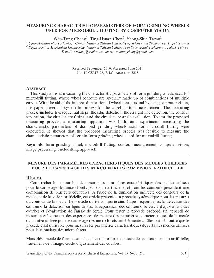
1 INTRODUCTION

Microdrills are precision microtools frequently used by the electric and semiconductorindustries to machine microholes in printed circuit boards (PCBs). Nowadays, most microdrillproducts are of nominal diameters ranging between 0.05 and 0.45 mm [1,2]. In microdrillmanufacture, the fluting process, a special type of form grinding process, must be performed tomachine helical flutes in microdrills. The helical flutes are necessary to provide space for chipremoval in drilling operations. Figure 1 shows the schematic diagram of the fluting process, inwhich the drill body (a cylindrical workpiece) of a microdrill is ground by a form grinding wheelwith specially designed wheel contour. To form helical flutes in the drill body, a relative screwmotion between the microdrill and the form grinding wheel is prescribed. To this end, both themicrodrill and the form grinding wheel rotate around their axes with a relative translation alongthe axis of the microdrill being generated. Based on such a relative screw motion, someprecision machines have been designed exclusively for microdrill fluting. The mathematicalmodeling and sensitivity analysis of the fluting process for microdrills have been investigated byKang [3], which can be helpful to the theoretical contour design of the form grinding wheel andthe parameter setting of fluting machines. The wheel contour accuracy of the form grindingwheel will strongly influence the geometric correctness of ground helical flutes in microdrills.Thus, the wheel contour must be regularly dressed and then accurately measured in order toensure quality of microdrill production. Using a coordinate measuring machine (CMM) or anoptical comparator to measure the wheel contour accuracy of grinding wheels are traditionalmethods. However, because the grinding wheel contours used for microdrill fluting are tiny andusually with non-regular geometry, it is difficult to measure their wheel contour accuracythrough the use of the traditional measuring methods. Therefore, alternative means for dealingwith the measuring task must be developed.

In recent years, using computer vision to measure or monitor the grinding wheel has beenstudied by several researchers [4–9]. Sodhi and Tiliouine [4] utilize a charged couple device(CCD) camera to acquire digital images of the speckle patterns caused by impinging a laserbeam on a ground surface, the surface roughness and the condition of the grinding wheel arethen evaluated through the information on the acquired images. Fan et al. [5] develop an on-line

Fig. 1. Schematic diagram of the fluting process for a microdrill.


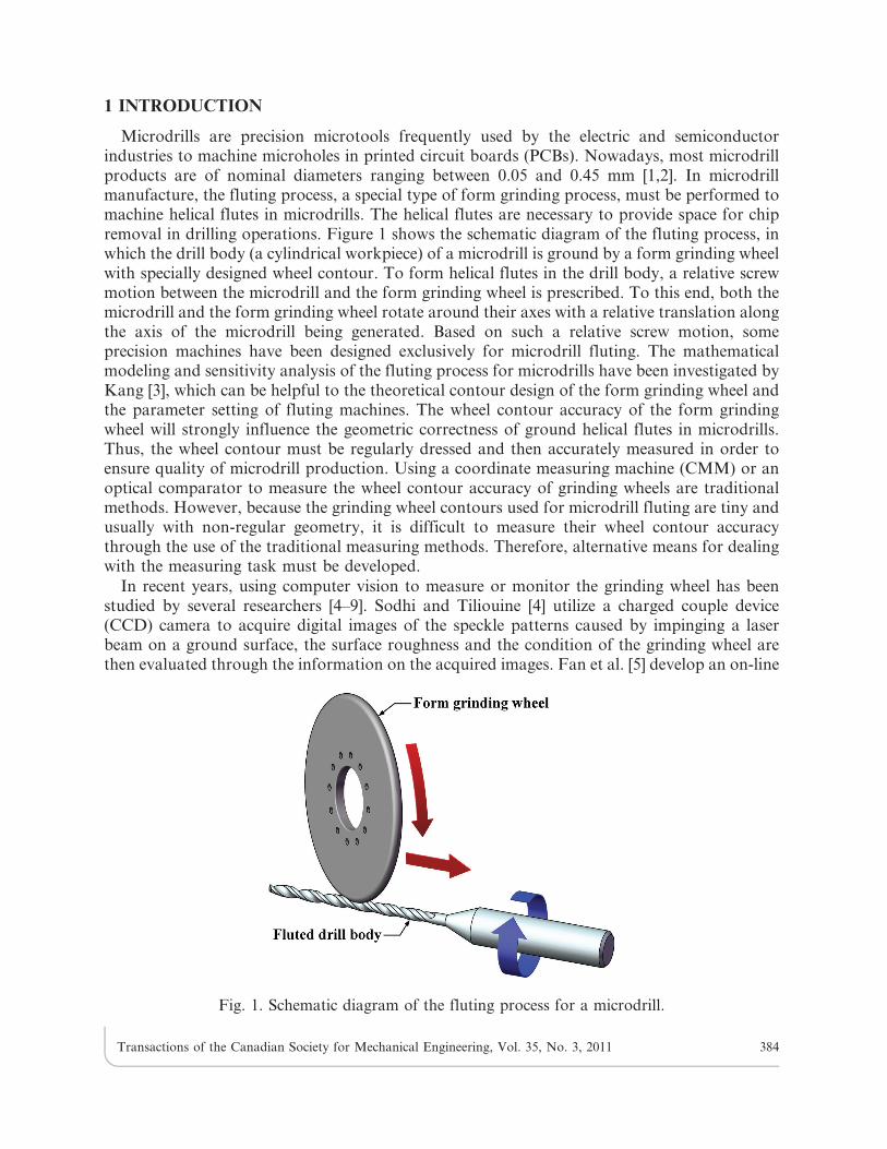
non-contact system to measure the wear of a form grinding wheel by directly capturing digitalimages of the grinding wheel edge with the use of a CCD camera. Lachance et al. [6] as well asFeng and Chen [7] use CCD cameras to directly capture digital images of the grinding wheelsurface and then evaluate the surface condition of grinding wheels. Su and Tarng [8] propose anindirect method of measuring the wear of form grinding wheels with the use of computer vision.Their method involves using a thin plate specimen ground to yield a two-dimensional contour inorder to duplicate the three-dimensional topography of the form grinding wheel, as shown inFig. 2. A CCD camera is then used to capture digital images of the ground contour of thespecimen for indirectly evaluating the wear of the wheel contour. Chen et al. [9], following theconcept of the indirect duplication of wheel contours [8], develop a contour matching method toexamine the contour accuracy of grinding wheels. The contour matching method is based oncalculating the relative deviations between the theoretical and inspected wheel contours with theuse of some optimization methods. The above studies show that computer vision technologyshould be increasingly important in the applications of grinding wheel measurement andmonitoring.

Based on computer vision technology, this study aims at measuring the characteristicparameters of form grinding wheels used for microdrill fluting, whose wheel contours arespecially made up of combinations of multiple curves. In this paper, the means of the indirectduplication of wheel contours [8,9], as shown in Fig. 2, is equally applied to yield a two-dimensional contour representing the form grinding wheel. Based on the captured computerimage of the yielded two-dimensional contour, a systematic process for the wheel contourmeasurement is then developed with the use of image processing algorithms. To test thefeasibility of the proposed measuring process, a measuring apparatus was built, andexperiments measuring the characteristic parameters of form grinding wheels used formachining helical flutes in microdrills were conducted.

2 THEORETICAL CONTOUR OF THE FORM GRINDING WHEEL

In this study, a systematic measuring process is to be developed for inspecting form grindingwheels used for machining helical flutes in some microdrill products. In order to measure the

Fig. 2. Schematic diagram of duplicating the topographical profile of the form grinding wheel byusing a thin plate specimen ground to yield a contour.


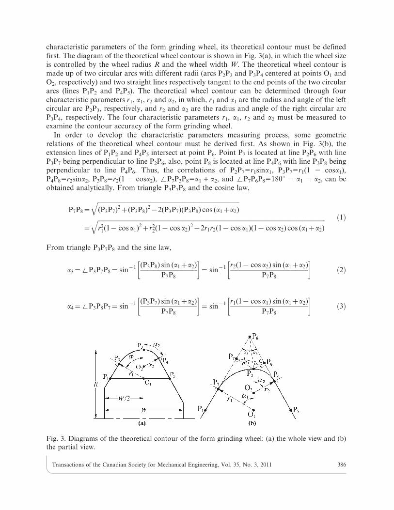
characteristic parameters of the form grinding wheel, its theoretical contour must be definedfirst. The diagram of the theoretical wheel contour is shown in Fig. 3(a), in which the wheel sizeis controlled by the wheel radius R and the wheel width W. The theoretical wheel contour ismade up of two circular arcs with different radii (arcs P2P3 and P3P4 centered at points O1 andO2, respectively) and two straight lines respectively tangent to the end points of the two circulararcs (lines P1P2 and P4P5). The theoretical wheel contour can be determined through fourcharacteristic parameters r1, a1, r2 and a2, in which, r1 and a1 are the radius and angle of the leftcircular arc P2P3, respectively, and r2 and a2 are the radius and angle of the right circular arcP3P4, respectively. The four characteristic parameters r1, a1, r2 and a2 must be measured toexamine the contour accuracy of the form grinding wheel.

In order to develop the characteristic parameters measuring process, some geometricrelations of the theoretical wheel contour must be derived first. As shown in Fig. 3(b), theextension lines of P1P2 and P4P5 intersect at point P6. Point P7 is located at line P2P6 with lineP3P7 being perpendicular to line P2P6, also, point P8 is located at line P4P6 with line P3P8 beingperpendicular to line P4P6. Thus, the correlations of P2P75r1sina1, P3P75r1(1 2 cosa1),P4P85r2sina2, P3P85r2(1 2 cosa2), %P7P3P85a1 + a2, and %P7P6P85180u 2 a1 2 a2, can beobtained analytically. From triangle P3P7P8 and the cosine law,

P7P8~

ffiffiffiffiffiffiffiffiffiffiffiffiffiffiffiffiffiffiffiffiffiffiffiffiffiffiffiffiffiffiffiffiffiffiffiffiffiffiffiffiffiffiffiffiffiffiffiffiffiffiffiffiffiffiffiffiffiffiffiffiffiffiffiffiffiffiffiffiffiffiffiffiffiffiffiffiffiffiffiffiffiffiffiffiffiffiffiffiffiffiffiffi(P3P7)2z(P3P8)2{2(P3P7)(P3P8) cos (a1za2)

q

~

ffiffiffiffiffiffiffiffiffiffiffiffiffiffiffiffiffiffiffiffiffiffiffiffiffiffiffiffiffiffiffiffiffiffiffiffiffiffiffiffiffiffiffiffiffiffiffiffiffiffiffiffiffiffiffiffiffiffiffiffiffiffiffiffiffiffiffiffiffiffiffiffiffiffiffiffiffiffiffiffiffiffiffiffiffiffiffiffiffiffiffiffiffiffiffiffiffiffiffiffiffiffiffiffiffiffiffiffiffiffiffiffiffiffiffiffiffiffiffiffiffiffiffiffiffiffiffiffiffiffiffiffiffiffiffiffiffiffiffiffiffiffiffiffiffiffiffiffir2

1(1{ cos a1)2zr22(1{ cos a2)2{2r1r2(1{ cos a1)(1{ cos a2) cos (a1za2)

q ð1Þ

From triangle P3P7P8 and the sine law,

a3~%P3P7P8~ sin{1 (P3P8) sin (a1za2)

P7P8

� �~ sin{1 r2(1{ cos a2) sin (a1za2)

P7P8

� �ð2Þ

a4~%P3P8P7~ sin{1 (P3P7) sin (a1za2)

P7P8

� �~ sin{1 r1(1{ cos a1) sin (a1za2)

P7P8

� �ð3Þ

Fig. 3. Diagrams of the theoretical contour of the form grinding wheel: (a) the whole view and (b)the partial view.


Then, from triangle P6P7P8 and the sine law,

P6P7~(P7P8) sin (900{a4)

sin (1800{a1{a2)~(P7P8) cos a4 csc (a1za2) ð4Þ

P6P8~(P7P8) sin (900{a3)

sin (1800{a1{a2)~(P7P8) cos a3 csc (a1za2) ð5Þ

Therefore,

P2P6~P2P7zP6P7~r1 sin a1z(P7P8) cos a4 csc (a1za2) ð6Þ

P4P6~P4P8zP6P8~r2 sin a2z(P7P8) cos a3 csc (a1za2) ð7Þ

Also, from right-angle triangle P3P6P7,

P3P6~

ffiffiffiffiffiffiffiffiffiffiffiffiffiffiffiffiffiffiffiffiffiffiffiffiffiffiffiffiffiffiffiffiffiffiffi(P3P7)2z(P6P7)2

q~

ffiffiffiffiffiffiffiffiffiffiffiffiffiffiffiffiffiffiffiffiffiffiffiffiffiffiffiffiffiffiffiffiffiffiffiffiffiffiffiffiffiffiffiffiffiffiffiffiffiffiffiffiffiffiffiffiffiffiffiffiffiffiffiffiffiffiffiffiffiffiffiffiffiffiffiffiffiffiffiffiffiffiffiffiffiffiffiffiffir2

1(1{ cos a1)2z(P7P8)2 cos2 a4 csc2 (a1za2)

qð8Þ

a5~%P3P6P7~ tan{1 P3P7

P6P7

� �~ tan{1 r1(1{ cos a1)

(P7P8) cos a4 csc (a1za2)

� �ð9Þ

On the other hand, from right-angle triangle P3P6P8,

P3P6~

ffiffiffiffiffiffiffiffiffiffiffiffiffiffiffiffiffiffiffiffiffiffiffiffiffiffiffiffiffiffiffiffiffiffiffi(P3P8)2z(P6P8)2

q~

ffiffiffiffiffiffiffiffiffiffiffiffiffiffiffiffiffiffiffiffiffiffiffiffiffiffiffiffiffiffiffiffiffiffiffiffiffiffiffiffiffiffiffiffiffiffiffiffiffiffiffiffiffiffiffiffiffiffiffiffiffiffiffiffiffiffiffiffiffiffiffiffiffiffiffiffiffiffiffiffiffiffiffiffiffiffiffiffiffir2

2(1{ cos a2)2z(P7P8)2 cos2 a3 csc2 (a1za2)

qð10Þ

a6~%P3P6P8~ tan{1 P3P8

P6P8

� �~ tan{1 r2(1{ cos a2)

(P7P8) cos a3 csc (a1za2)

� �ð11Þ

As shown in above equations, if the values of the four characteristic parameters r1, a1, r2 and a2

are given, the other geometric terms dependent on them can be determined correspondingly.

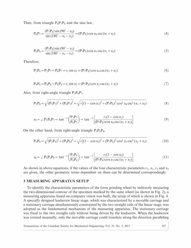
3 MEASURING APPARATUS SETUP

To identify the characteristic parameters of the form grinding wheel by indirectly measuringthe two-dimensional contour of the specimen marked by the same wheel (as shown in Fig. 2), ameasuring apparatus based on computer vision was built, the setup of which is shown in Fig. 4.A specially designed leadscrew linear stage, which was characterized by a movable carriage anda stationary carriage simultaneously constrained by the two straight rails of the linear stage, wasadopted as the fundamental mechanism of the measuring apparatus. The stationary carriagewas fixed to the two straight rails without being driven by the leadscrew. When the leadscrewwas rotated manually, only the movable carriage could translate along the direction paralleling


the straight rails. (The translating direction of the movable carriage is called the Z-direction ofthe measuring apparatus). An Imaging Source DMK41BUC02 complementary metal-oxide-semiconductor (CMOS) camera coupled with a Navitar 12X telecentric lens was mounted on alens tube holder and a backlighting board was prepared as the light source for the vision system.The measured specimen, made of high-carbon steel, was placed on a vertical observation stageformed by a miniature X-Y table with a magnetic fixture that magnetizes the specimen. The lenstube holder was fixed to the movable carriage, while the backlighting board and the verticalobservation stage were fixed to the stationary carriage. Through the translation of the movablecarriage, focusing adjustment of the vision system could be performed. The CMOS camera wasconnected to a personal computer (not shown in the figure) using the universal serial bus (USB)port.

For the measurement, the specimen was placed between the backlighting board and thetelecentric lens. In order to enhance the contrast of the vision system, red backlighting waschosen. The red light projecting on the back of the specimen created a silhouette in front of thetelecentric lens, which was sensed and captured by the CMOS camera, then stored by thepersonal computer as a digital image. The captured digital image consisted of a 1280|1024array of pixels of grayscale intensity values ranging from 0 to 255. By applying the spatialcalibration method that had been used by Chen et al. [9], the conversion factor of the captureddigital image corresponding to its real world dimension was found to be 0.756 mm/pixel. Also,

Fig. 4. The built measuring apparatus.


by employing the subpixel localization algorithm [9–11], the built computer vision system couldachieve an estimated resolution of 1/25 of a pixel [10], that is, 0.0302 mm.

4 THE CHARACTERISTIC PARAMETERS MEASURING PROCESS

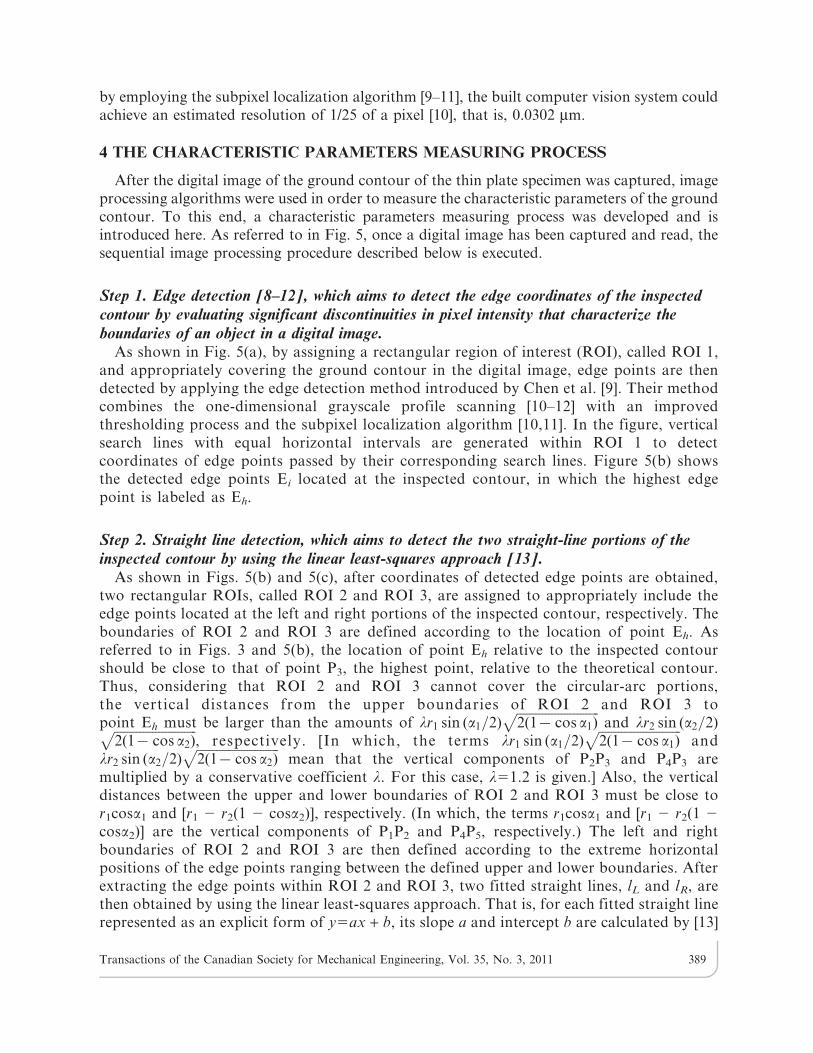
After the digital image of the ground contour of the thin plate specimen was captured, imageprocessing algorithms were used in order to measure the characteristic parameters of the groundcontour. To this end, a characteristic parameters measuring process was developed and isintroduced here. As referred to in Fig. 5, once a digital image has been captured and read, thesequential image processing procedure described below is executed.

Step 1. Edge detection [8–12], which aims to detect the edge coordinates of the inspectedcontour by evaluating significant discontinuities in pixel intensity that characterize theboundaries of an object in a digital image.

As shown in Fig. 5(a), by assigning a rectangular region of interest (ROI), called ROI 1,and appropriately covering the ground contour in the digital image, edge points are thendetected by applying the edge detection method introduced by Chen et al. [9]. Their methodcombines the one-dimensional grayscale profile scanning [10–12] with an improvedthresholding process and the subpixel localization algorithm [10,11]. In the figure, verticalsearch lines with equal horizontal intervals are generated within ROI 1 to detectcoordinates of edge points passed by their corresponding search lines. Figure 5(b) showsthe detected edge points Ei located at the inspected contour, in which the highest edgepoint is labeled as Eh.

Step 2. Straight line detection, which aims to detect the two straight-line portions of theinspected contour by using the linear least-squares approach [13].

As shown in Figs. 5(b) and 5(c), after coordinates of detected edge points are obtained,two rectangular ROIs, called ROI 2 and ROI 3, are assigned to appropriately include theedge points located at the left and right portions of the inspected contour, respectively. Theboundaries of ROI 2 and ROI 3 are defined according to the location of point Eh. Asreferred to in Figs. 3 and 5(b), the location of point Eh relative to the inspected contourshould be close to that of point P3, the highest point, relative to the theoretical contour.Thus, considering that ROI 2 and ROI 3 cannot cover the circular-arc portions,the vertical distances from the upper boundaries of ROI 2 and ROI 3 topoint Eh must be larger than the amounts of lr1 sin (a1=2)

ffiffiffiffiffiffiffiffiffiffiffiffiffiffiffiffiffiffiffiffiffiffiffiffiffiffi2(1{ cos a1)

pand lr2 sin (a2=2)ffiffiffiffiffiffiffiffiffiffiffiffiffiffiffiffiffiffiffiffiffiffiffiffiffiffi

2(1{ cos a2)p

, respectively. [In which, the terms lr1 sin (a1=2)ffiffiffiffiffiffiffiffiffiffiffiffiffiffiffiffiffiffiffiffiffiffiffiffiffiffi2(1{ cos a1)

pand

lr2 sin (a2=2)ffiffiffiffiffiffiffiffiffiffiffiffiffiffiffiffiffiffiffiffiffiffiffiffiffiffi2(1{ cos a2)

pmean that the vertical components of P2P3 and P4P3 are

multiplied by a conservative coefficient l. For this case, l51.2 is given.] Also, the verticaldistances between the upper and lower boundaries of ROI 2 and ROI 3 must be close tor1cosa1 and [r1 2 r2(1 2 cosa2)], respectively. (In which, the terms r1cosa1 and [r1 2 r2(1 2

cosa2)] are the vertical components of P1P2 and P4P5, respectively.) The left and rightboundaries of ROI 2 and ROI 3 are then defined according to the extreme horizontalpositions of the edge points ranging between the defined upper and lower boundaries. Afterextracting the edge points within ROI 2 and ROI 3, two fitted straight lines, lL and lR, arethen obtained by using the linear least-squares approach. That is, for each fitted straight linerepresented as an explicit form of y5ax + b, its slope a and intercept b are calculated by [13]


a~

nPni~1

xEiyEi

{Pni~1

xEi

Pni~1

yEi

nPni~1

x2Ei

{Pni~1

xEi

� �2ð12Þ

Fig. 5. An illustrative example of the sequential procedure for measuring the characteristicparameters of an inspected form grinding wheel.


b~

Pni~1

x2Ei

Pni~1

yEi{Pni~1

xEi

Pni~1

xEiyEi

nPni~1

x2Ei

{Pni~1

xEi

� �2ð13Þ

where xEiand yEi

represent the X- and Y-components of any detected edge point Ei (for i51,2, …, n) within ROI 2 or ROI 3, respectively.

Step 3. Contour separation, which aims to separate the two circular-arc portions and the twostraight-line portions from the inspected contour by applying the concept of the region ofuncertainty (ROU).

For the theoretical contour shown in Fig. 3, the two circular-arc portions and the twostraight-line portions are separated by the locations of points P2, P3 and P4, respectively.Likewise, for the inspected contour, locations of approximate points ~PP2, ~PP3 and ~PP4 shown inFig. 5(d) can be found in order to aid the contour separation. As shown in Fig. 5(c), the twofitted straight lines, lL and lR, intersect at point ~PP6. The location of point ~PP6 relative to theinspected contour should be close to that of point P6 relative to the theoretical contour. Whenthe coordinate of point ~PP6 is determined, the position of point ~PP2 is calculated by finding a pointon line lL that satisfies the correlation of ~PP2

~PP6~P2P6, where P2P6 can be calculated by using Eq.(6) with the values of the theoretical characteristic parameters r1, a1, r2 and a2 being given. Also,the position of point ~PP4 is calculated by finding a point on line lR that satisfies the correlation of~PP4

~PP6~P4P6, where P4P6 can be calculated by using Eq. (7). Then, by using Eq. (9) and theinformation on line lL and point ~PP6, an auxiliary line passing through point ~PP6 and forming anincluded angle of a5 with line lL can be determined; similarly, by using Eq. (11) and theinformation on line lR and point ~PP6, another auxiliary line passing through point ~PP6 andforming an included angle of a6 with line lR can be determined. On each auxiliary line, anauxiliary point with a relative distance of P3P6 to point ~PP6 can be found by using Eq. (8) or Eq.(10). The position of point ~PP3 is thus obtained by averaging the coordinates of the two auxiliarypoints. However, since there must be slight deviations between the inspected and theoreticalcontours, points ~PP2, ~PP3 and ~PP4 cannot be regarded as exact contour separation points for theinspected contour. The exact contour separation points should be closed to points ~PP2, ~PP3 and ~PP4

but with uncertainty. Therefore, the concept of region of uncertainty (ROU) can be applied toperform the contour separation. As shown in Fig. 5(d), by assigning three ROUs, ROU 1, ROU2 and ROU 3, centered at points ~PP2, ~PP3 and ~PP4, respectively, edge points within the ROUs areregarded as contour separation points. The remaining edge points are then separated into thetwo circular-arc portions and the two straight-line portions. In this case, a ROU is simplydefined by assigning the left and right horizontal distances from a calculated approximate point.

Step 4. Circular arc fitting, which aims to measure the radii of the two circular arcs of theinspected contour by applying the so-called circle-fitting approaches (CFAs) with theinformation on the detected edge points belonging to the two circular-arc portions.

This step is considered a critical task of the measuring process. Both the circle-fittingapproaches (CFAs) based on least-squares (LS) [5,8] and genetic algorithm (GA) [14–18] areadopted in this study in order to evaluate their adaptability for the measurement. Bothapproaches are briefly described below.


Least-squares circle-fitting approach (LSCFA):Considering a group of detected edge points Eis (for i51, 2, …, n) belonging to a circular-arc

portion, by applying the linear least-squares approach for circle fitting [5,8], three coefficientsC1, C2 and C3 of the equation of the fitted circle can be solved by

C1

C2

C3

8><>:

9>=>;~

Pni~1

x2Ei

Pni~1

xEiyEi

Pni~1

xEi

Pni~1

xEiyEi

Pni~1

y2Ei

Pni~1

yEi

Pni~1

xEi

Pni~1

yEin

266666664

377777775

{1

{Pni~1

xEi(x2

Eizy2

Ei)

{Pni~1

yEi(x2

Eizy2

Ei)

{Pni~1

(x2Ei

zy2Ei

)

8>>>>>>><>>>>>>>:

9>>>>>>>=>>>>>>>;

ð14Þ

Then, the radius of the fitted circle, ~rr, can be calculated by

~rr~

ffiffiffiffiffiffiffiffiffiffiffiffiffiffiffiffiffiffiffiffiffiffiffiffiffiffiffiffiffiC2

1zC22{4C3

q2

ð15Þ

and the coordinate of the circular center, ~OO, can be calculated by

x~OO

y~OO

� �~

{C1=2

{C2=2

� �ð16Þ

Genetic algorithm circle-fitting approach (GACFA):Considering a group of detected edge points Eis (for i51, 2, …, n) belonging to a circular-arc

portion, by randomly choosing three edge points Ej, Ek and El in them, a candidate circlepassing through the three edge points can be determined [18]. The coordinate of the circularcenter, ~OO, can be calculated by

x~OO

y~OO

� �~

(x2Ek

zy2Ek

{x2Ej

{y2Ej

)(yEl{yEj

){(x2El

zy2El

{x2Ej

{y2Ej

)(yEk{yEj

)

2½(xEk{xEj

)(yEl{yEj

){(xEl{xEj

)(yEk{yEj

)�

(x2El

zy2El

{x2Ej

{y2Ej

)(xEk{xEj

){(x2Ek

zy2Ek

{x2Ej

{y2Ej

)(xEl{xEj

)

2½(xEk{xEj

)(yEl{yEj

){(xEl{xEj

)(yEk{yEj

)�

8>>>>><>>>>>:

9>>>>>=>>>>>;

ð17Þ

Then, the radius of the candidate circle, ~rr, can be calculated by

~rr~

ffiffiffiffiffiffiffiffiffiffiffiffiffiffiffiffiffiffiffiffiffiffiffiffiffiffiffiffiffiffiffiffiffiffiffiffiffiffiffiffiffiffiffiffiffiffiffiffiffi(xEk

{x~OO)2z(yEk{y~OO)2

qð18Þ

A transformation operation T between the three indices of the randomly chosen points, (j, k, l),and the determined candidate circle, (x~OO, y~OO, ~rr), can be represented by


(x~OO, y~OO, ~rr)~T(j, k, l) ð19Þ

For the use of GA, the three indices of the randomly chosen edge points, (j, k, l), are consideredthe design variables and encoded to binary strings as genes of a chromosome. For the circle-fitting approach, a fitness function to be minimized can be defined by

F (x~OO, y~OO, ~rr)~F (T(j, k, l))~Xn

i~1

ffiffiffiffiffiffiffiffiffiffiffiffiffiffiffiffiffiffiffiffiffiffiffiffiffiffiffiffiffiffiffiffiffiffiffiffiffiffiffiffiffiffiffiffiffiffiffi(xEi

{x~OO)2z(yEi{y~OO)2

q{~rr

ð20Þ

which means to minimize the sum of absolute radial deviations between the determinedcandidate circle and all detected edge points Eis. For the evolution process, each chromosome is21 bits in length and the population size is 10. The reproduction operator used is thetournament selection. The crossover operator used is the one-cut-point method with a crossoverprobability of 0.9. The mutation operator used is the one-bit inversion with a mutationprobability of 0.9. For each generation (iteration), the old population is totally replaced by thenew mated one. The stopping criteria is when the number of generations being larger than10000. After performing above GA-based optimization, the best-fit circle with the use of threedetected edge points can be found.

As shown in Fig. 5(e), through using the LSCFA or the GACFA, two fitted circular arcs(FCAs), FCA 1 and FCA 2, can be determined, and their radii, ~rr1 and ~rr2, and circular centers,~OO1 and ~OO2, can also be obtained. The evaluated radii, ~rr1 and ~rr2, are regarded as the measuredcircular arc radii of the inspected contour.

Step 5. Circular arc angle evaluation, which aims to measure the angles of the two circular arcsof the inspected contour by using the information on the two FCAs.

After FCA 1 and FCA 2 are determined in Step 4, the information on their circular centers,~OO1 and ~OO2, are adopted to evaluate their circular arc angles. As shown in Fig. 5(f), by finding aline lO passing through points ~OO1 and ~OO2, the left circular arc angle ~aa1 can be determined bycalculating the subtending angle between lines lO and mL, where line mL is perpendicular to linelL and passes through point ~OO1. Similarly, the right circular arc angle ~aa2 can be determined bycalculating the subtending angle between lines lO and mR, where line mR is perpendicular to linelR and passes through point ~OO2. The evaluated angles, ~aa1 and ~aa2, are regarded as the measuredcircular arc angles of the inspected contour.

5 EXPERIMENTAL RESULTS AND DISCUSSION

Experiments in which the characteristic parameters of form grinding wheels were measuredwere conducted in order to test the feasibility and effectiveness of the proposed measuringprocess.

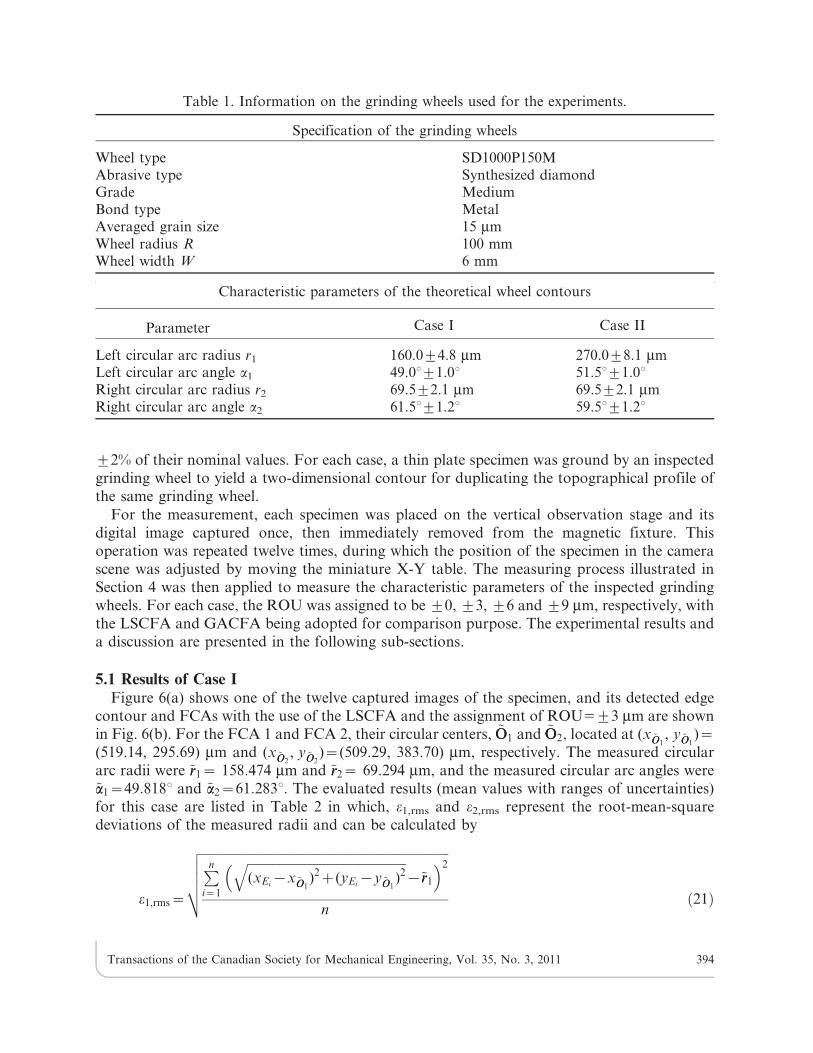
In this study, diamond grinding wheels used for machining helical flutes in some Topointmicrodrill test products were measured. The information on the form grinding wheels used forthe experiments is listed in Table 1, in which, Case I refers to the grinding wheel used formachining microdrills with nominal diameters of 0.25 mm, and Case II refers to that used formachining microdrills with nominal diameters of 0.35 mm. As shown in Table 1, tolerances ofthe circular arc radii are ¡3% of their nominal values, and those of the circular arc angles are


¡2% of their nominal values. For each case, a thin plate specimen was ground by an inspectedgrinding wheel to yield a two-dimensional contour for duplicating the topographical profile ofthe same grinding wheel.

For the measurement, each specimen was placed on the vertical observation stage and itsdigital image captured once, then immediately removed from the magnetic fixture. Thisoperation was repeated twelve times, during which the position of the specimen in the camerascene was adjusted by moving the miniature X-Y table. The measuring process illustrated inSection 4 was then applied to measure the characteristic parameters of the inspected grindingwheels. For each case, the ROU was assigned to be ¡0, ¡3, ¡6 and ¡9 mm, respectively, withthe LSCFA and GACFA being adopted for comparison purpose. The experimental results anda discussion are presented in the following sub-sections.

5.1 Results of Case IFigure 6(a) shows one of the twelve captured images of the specimen, and its detected edge

contour and FCAs with the use of the LSCFA and the assignment of ROU5¡3 mm are shownin Fig. 6(b). For the FCA 1 and FCA 2, their circular centers, ~OO1 and ~OO2, located at (x~OO1

, y~OO1)~

(519.14, 295.69) mm and (x~OO2, y~OO2

)~(509.29, 383.70) mm, respectively. The measured circulararc radii were ~rr1~ 158.474 mm and ~rr2~ 69.294 mm, and the measured circular arc angles were~aa1~49:818u and ~aa2~61:283u. The evaluated results (mean values with ranges of uncertainties)for this case are listed in Table 2 in which, e1,rms and e2,rms represent the root-mean-squaredeviations of the measured radii and can be calculated by

e1,rms~

ffiffiffiffiffiffiffiffiffiffiffiffiffiffiffiffiffiffiffiffiffiffiffiffiffiffiffiffiffiffiffiffiffiffiffiffiffiffiffiffiffiffiffiffiffiffiffiffiffiffiffiffiffiffiffiffiffiffiffiffiffiffiffiffiffiffiffiffiffiffiffiffiffiffiffiffiffiffiPni~1

ffiffiffiffiffiffiffiffiffiffiffiffiffiffiffiffiffiffiffiffiffiffiffiffiffiffiffiffiffiffiffiffiffiffiffiffiffiffiffiffiffiffiffiffiffiffiffiffiffiffi(xEi

{x~OO1)2z(yEi

{y~OO1)2

q{~rr1

�2

n

vuuutð21Þ

Table 1. Information on the grinding wheels used for the experiments.

Specification of the grinding wheels

Wheel type SD1000P150MAbrasive type Synthesized diamondGrade MediumBond type MetalAveraged grain size 15 mmWheel radius R 100 mmWheel width W 6 mm

Characteristic parameters of the theoretical wheel contours

Parameter Case I Case II

Left circular arc radius r1 160.0¡4.8 mm 270.0¡8.1 mmLeft circular arc angle a1 49.0u¡1.0u 51.5u¡1.0uRight circular arc radius r2 69.5¡2.1 mm 69.5¡2.1 mmRight circular arc angle a2 61.5u¡1.2u 59.5u¡1.2u


e2,rms~

ffiffiffiffiffiffiffiffiffiffiffiffiffiffiffiffiffiffiffiffiffiffiffiffiffiffiffiffiffiffiffiffiffiffiffiffiffiffiffiffiffiffiffiffiffiffiffiffiffiffiffiffiffiffiffiffiffiffiffiffiffiffiffiffiffiffiffiffiffiffiffiffiffiffiffiffiffiffiPni~1

ffiffiffiffiffiffiffiffiffiffiffiffiffiffiffiffiffiffiffiffiffiffiffiffiffiffiffiffiffiffiffiffiffiffiffiffiffiffiffiffiffiffiffiffiffiffiffiffiffiffi(xEi

{x~OO2)2z(yEi

{y~OO2)2

q{~rr2

�2

n

vuuutð22Þ

As seen from Table 2, the mean values of the measured parameters with the assignment ofROU5¡3 mm all lay within their specified tolerance bands, although the relative differencebetween the mean measured values of ~rr1 by using the two CFAs was about 1.3 mm. For theLSCFA, by using the three-standard-deviation-band approach, the maximum uncertainties fellwithin the ranges of ¡0.957 mm and +0:389u when the ROU was assigned to be ¡9 mm. Forthe GACFA, the maximum uncertainties fell within the ranges of ¡3.328 mm and +0:927uwhen the ROU was assigned to be ¡9 mm. No matter how large the range of ROU being

Fig. 6. Characteristic parameters measured result for Case I: (a) the captured digital image of theinspected specimen and (b) the detected edge and the fitted circular arcs.


assigned, most uncertainties related to the GACFA still kept about 2 to 3.5 times those relatedto the LSCFA. Nevertheless, for both CFAs, the mean values and uncertainties of either e1,rms

or e2,rms were quite close to each other and had less significance on influencing the measurementof the circular arc radii.

Figure 7 shows the mean measured values of the four characteristic parameters with respect toassigned ROUs. As shown in Fig. 7(a), the mean measured radius ~rr1,avg related to the LSCFA hada decreased trend with the increased ROU, while that related to the GACFA increased whenROU was larger than ¡3 mm. On the other hand, as shown in Fig. 7(b), the mean measuredradius ~rr2,avg related to both CFAs had quite similar trends and magnitudes. When ROU5¡9 mm,the magnitudes of ~rr2,avg were less than its lower bound (67.4 mm). Such a situation showed that theassignment of ROU5¡9 mm was not appropriate for the measurement of the right circular arc ofthe inspected contour. In Figs. 7(c) and 7(d) , the mean measured angles ~aa1,avg and ~aa2,avg related tothe LSCFA had obvious variations, while those related to the GACFA had relatively stabletrends. When ROU was larger than the range of ¡6 mm, the LSCFA could not provide sufficientadaptability for measuring the circular arc angles. That is, the GACFA was more reliable than theLSCFA for measuring the circular arc angles for this case.

5.2 Results of Case IIFor this case, one of the twelve captured images of the specimen is shown in Fig. 8(a), and its

detected edge contour and FCAs with the use of the LSCFA and the assignment ofROU5¡3 mm are shown in Fig. 8(b). For the FCA 1 and FCA 2, their circular centers locatedat (x~OO1

, y~OO1)5(545.61, 207.82) mm and (x~OO2

, y~OO2)5(546.34, 406.57) mm, respectively. The

measured circular arc radii were ~rr1~267.976 mm and ~rr2~ 68.843 mm, and the measured circulararc angles were ~aa1~51:609u and ~aa2~59:148u. The evaluated results (mean values with ranges ofuncertainties) for this case are listed in Table 3, as similar to those listed in Table 2. As shown inTable 3, the mean values of the measured parameters with the assignment of ROU5¡3 mm alllay within their specified tolerance bands, however, the relative difference between the meanmeasured values of ~rr2 by using the two CFAs was about 2.6 mm. For the LSCFA, the maximumuncertainties fell within the ranges of ¡1.227 mm and +0:166u when the ROU was assigned tobe ¡9 mm. For the GACFA, the maximum uncertainties fell within the ranges of ¡1.994 mmand +0:410u when the ROU was assigned to be ¡9 mm. For this case, most uncertaintiesrelated to the GACFA kept about 1.5 to 3 times those related to the LSCFA. Also, the meanvalues and uncertainties of either e1,rms or e2,rms related to both CFAs were quite close to eachother and could be ignored.

Table 2. Evaluated results for Case I.

CFA ~rr1(mm) ~rr2(mm) ~aa1(deg) ~aa2(deg) e1,rms(mm) e2,rms(mm)

ROU5

¡0 mmLS 159.214¡0.843 70.235¡0.352 49.529¡0.270 61.571¡0.216 0.381¡0.015 0.141¡0.014GA 160.271¡2.453 70.341¡0.770 49.299¡0.597 61.801¡0.602 0.388¡0.017 0.143¡0.015

ROU5

¡3 mmLS 158.281¡0.881 69.569¡0.542 49.774¡0.286 61.326¡0.250 0.361¡0.014 0.138¡0.017GA 159.605¡2.704 69.950¡1.165 49.384¡0.821 61.716¡0.818 0.366¡0.015 0.140¡0.019

ROU5

¡6 mmLS 157.085¡0.902 68.345¡0.693 50.269¡0.335 60.831¡0.296 0.346¡0.014 0.134¡0.018GA 161.564¡2.568 68.126¡1.031 49.107¡0.592 61.993¡0.616 0.353¡0.014 0.137¡0.018

ROU5

¡9 mmLS 156.368¡0.957 65.820¡0.812 50.985¡0.389 60.116¡0.348 0.323¡0.014 0.117¡0.016GA 164.464¡3.328 65.045¡0.952 48.997¡0.927 62.103¡0.878 0.354¡0.025 0.122¡0.016


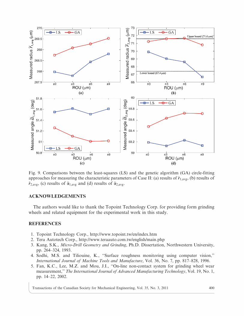
Figure 9 shows the mean measured values of the four characteristic parameters with respect toassigned ROUs. As shown in Fig. 9(a), the mean measured radius ~rr1,avg related to both CFAs hadsimilar trends in substance, while their maximum relative difference occurring at ROU5¡3 mmwas about 1.3 mm. However, in Fig. 9(b), the mean measured radius ~rr2,avg related to both CFAshad quite different trends and magnitudes. The magnitudes of ~rr2,avg related to the GACFA werequite close to the upper bound (71.6 mm), while those related to the LSCFA appeared anobviously decreased trend with the increased ROU; their maximum relative difference occurringat ROU5¡9 mm was about 4.1 mm. In Figs. 9(c) and 9(d), the mean measured angles ~aa1,avg and~aa2,avg related to the GACFA had obvious variations, while those related to the LSCFA hadrelatively stable trends. Such situations were contrary to those appeared in Case I.

5.3 DiscussionFrom the experimental results, it can be found that the assignment of the range of the ROU

considerably influences the reasonability of the characteristic parameter measuring results.Assigning a larger range of the ROU leads to less edge points being considered in the circle

Fig. 7. Comparisons between the least-squares (LS) and the genetic algorithm (GA) circle-fittingapproaches for measuring the characteristic parameters of Case I: (a) results of ~rr1,avg, (b) results of~rr2,avg, (c) results of ~aa1,avg and (d) results of ~aa2,avg.


fitting, and thus results in certain unreasonable measuring results. For the two cases, theassignment of ROU5¡3 mm should be most appropriate for the measurement. When the rangeof the assigned ROU was larger than ¡6 mm, some measuring results could be consideredincorrect because of the elimination of some meaningful edge points for representing thecircular-arc portions of the inspected contour. Also, no matter how large the range of ROUbeing assigned, most uncertainties related to the GACFA kept about 1.5 to 3.5 times thoserelated to the LSCFA.

When the range of the assigned ROU was less than ¡6 mm, the maximum relative differencebetween the measured radii obtained by using the two CFAs was about 2.6 mm. That is, boththe LSCFA and GACFA were feasible to the measurement of the circular arc radii providedthat appropriate range of the ROU was assigned. In addition, for Case I, the use of the GACFAcould result in relatively stable results for the measurement of the circular arc angles ascompared with the use of the LSCFA. But, a contrary situation to a slighter extent appeared in

Fig. 8. Characteristic parameters measured result for Case II: (a) the captured digital image of theinspected specimen and (b) the detected edge and the fitted circular arcs.


Case II. In practice, the number of detected edge points belonging to the two circular-arcportions in Case I was less than that of Case II. Such a situation combining with the assignmentof a larger range of the ROU might contribute to a worse adaptability of using the LSCFA forthe measurement of the circular arc angles. However, the use of the GACFA involved muchiterative computation and was therefore more time-consuming than the use of the LSCFA. Insummary, with an appropriate range of the ROU being assigned, both the LSCFA andGACFA could achieve reasonable measuring results, but the use of the GACFA led torelatively lower efficiency as compared with the use of the LSCFA.

The feasibility and effectiveness of the proposed measuring process were verified throughexperiments. It must be emphasized that the presented measuring method was developed forinspecting form grinding wheels with specially designed contours used for microdrill fluting. Itdoes not intend to replace traditional methods of usual wheel contour measurement, such as theuse of a CMM or an optical comparator. Also, some commercially available vision systemscould replace the built measuring apparatus, in case they can achieve sufficient resolution andmeasuring accuracy.

6 CONCLUSIONS

With the aid of the indirect duplication of wheel contours [8,9] and by using computer visionand image processing algorithms, a characteristic parameter measuring process for inspectingform grinding wheels with specially designed contours used for microdrill fluting has beenintroduced in this study. The measuring process includes five sequential steps, which are theedge detection, the straight line detection, the contour separation, the circular arc fitting, andthe circular arc angle evaluation. For the step of contour separation, the concept of ROU hasbeen applied. For the step of circular arc fitting, both the LSCFA and the GACFA has beenadopted for comparison purpose. The proposed measuring process was tested by applying it toinspect diamond grinding wheels used for machining helical flutes in microdrills, and ameasuring apparatus was built for the experiments. From the experimental results, theproposed measuring process had shown its feasibility and effectiveness for the measurement ofthe characteristic parameters. With an appropriate range of the ROU being assigned, both theLSCFA and GACFA could achieve reasonable measuring results, but the use of the GACFAled to relatively lower efficiency as compared with the use of the LSCFA. In conclusion, thisstudy presents a feasible means for measuring the characteristic parameters of certain formgrinding wheels used for microdrill fluting.

Table 3. Evaluated results for Case II.

CFA ~rr1(mm) ~rr2(mm) ~aa1(deg) ~aa2(deg) e1,rms(mm) e2,rms(mm)

ROU5

¡0 mmLS 267.975¡0.493 69.899¡0.431 51.550¡0.093 59.190¡0.098 0.323¡0.011 0.287¡0.017GA 268.743¡1.312 71.242¡0.492 51.258¡0.174 59.482¡0.147 0.328¡0.014 0.303¡0.016

ROU5

¡3 mmLS 267.795¡0.483 69.020¡0.394 51.613¡0.081 59.126¡0.079 0.307¡0.014 0.290¡0.018GA 269.080¡1.388 71.595¡0.957 51.104¡0.242 59.636¡0.228 0.314¡0.019 0.306¡0.019

ROU5

¡6 mmLS 268.436¡0.535 68.615¡0.553 51.509¡0.097 59.231¡0.092 0.299¡0.015 0.292¡0.019GA 269.262¡1.479 71.677¡1.003 51.010¡0.275 59.729¡0.266 0.306¡0.022 0.313¡0.018

ROU5

¡9 mmLS 268.801¡0.567 66.675¡1.227 51.608¡0.166 59.132¡0.161 0.284¡0.015 0.295¡0.019GA 269.518¡1.536 70.807¡1.994 51.018¡0.410 59.722¡0.399 0.289¡0.015 0.317¡0.024


ACKNOWLEDGEMENTS

The authors would like to thank the Topoint Technology Corp. for providing form grindingwheels and related equipment for the experimental work in this study.

REFERENCES

1. Topoint Technology Corp., http://www.topoint.tw/en/index.htm

2. Tera Autotech Corp., http://www.teraauto.com.tw/english/main.php

3. Kang, S.K., Micro-Drill Geometry and Grinding, Ph.D. Dissertation, Northwestern University,

pp. 264–324, 1993.

4. Sodhi, M.S. and Tiliouine, K., ‘‘Surface roughness monitoring using computer vision,’’

International Journal of Machine Tools and Manufacture, Vol. 36, No. 7, pp. 817–828, 1996.

5. Fan, K.C., Lee, M.Z. and Mou, J.I., ‘‘On-line non-contact system for grinding wheel wear

measurement,’’ The International Journal of Advanced Manufacturing Technology, Vol. 19, No. 1,

pp. 14–22, 2002.

Fig. 9. Comparisons between the least-squares (LS) and the genetic algorithm (GA) circle-fittingapproaches for measuring the characteristic parameters of Case II: (a) results of ~rr1,avg, (b) results of~rr2,avg, (c) results of ~aa1,avg and (d) results of ~aa2,avg.


6. Lachance, S., Bauer, R. and Warkentin, A., ‘‘Application of region growing method to evaluatethe surface condition of grinding wheels,’’ International Journal of Machine Tools andManufacture, Vol. 44, No. 7–8, pp. 823–829, 2004.

7. Feng, Z. and Chen, X., ‘‘Image processing of the grinding wheel surface,’’ The International

Journal of Advanced Manufacturing Technology, Vol. 32, No. 5-6, pp. 452–458, 2007.8. Su, J.C. and Tarng, Y.S., ‘‘Measuring wear of the grinding wheel using machine vision,’’ The

International Journal of Advanced Manufacturing Technology, Vol. 31, No. 1, pp. 50–60, 2006.9. Chen, T.H., Chang, W.T., Shen, P.H. and Tarng, Y.S., ‘‘Examining the profile accuracy of

grinding wheels used for microdrill fluting by an image-based contour matching method,’’Proceedings of the Institution of Mechanical Engineers, Part B: Journal of Engineering

Manufacture, Vol. 224, No. 6, pp. 899–911, 2010.10. National Instrument Corp., NI Vision Concepts Manual, National Instrument Corp, pp. 11.1–

11.22, 2007.11. Jain, R., Kasturi, R. and Schunck, B.G., Machine Vision, McGraw-Hill, pp. 140–185, pp. 210–

2231995.12. Gonzalez, R.C. and Woods, R.E., Digital Image Processing, 2nd ed., Prentice-Hill, pp. 568–585,

2002.13. Faires, J.D. and Burden, R., Numerical Methods, 3nd ed., Thomson Learning, pp. 340–348,

2003.14. Holland, J.H., Adaptation in Natural and Artificial Systems, MIT Press, 1992.15. Goldberg, D.E., Genetic Algorithms in Search, Optimization, and Machine Learning, Addison-

Wesley Professional, 1989.16. Mitchell, M., An Introduction to Genetic Algorithms, MIT Press, 1996.17. Arora, J.S., Introduction to Optimum Design, 2nd ed., Elsevier Academic Press, pp. 531–541,

2004.18. Ayala-Ramirez, V., Garcia-Capulin, C.H., Perez-Garcia, A. and Sanchez-Yanez, R.E., ‘‘Circle

detection on images using genetic algorithms,’’ Pattern Recognition Letters, Vol. 27, No. 6,pp. 652–657, 2006.


measuring characteristic parameters of form grinding ... · industries to machine microholes in...

Documents