measures of dispersion - evirtualguruevirtualguru.com/books/ncert/11class/statistics... · ·...

1. INTRODUCTION

In the previous chapter, you havestudied how to sum up the data intoa single representative value. However,that value does not reveal thevariability present in the data. In thischapter you will study those

measures, which seek to quantifyvariability of the data.

Three friends, Ram, Rahim andMaria are chatting over a cup of tea.During the course of theirconversation, they start talking abouttheir family incomes. Ram tells themthat there are four members in hisfamily and the average income permember is Rs 15,000. Rahim says thatthe average income is the same in hisfamily, though the number of membersis six. Maria says that there are fivemembers in her family, out of whichone is not working. She calculates thatthe average income in her family too,is Rs 15,000. They are a little surprisedsince they know that Maria’s father isearning a huge salary. They go intodetails and gather the following data:

Measures of Dispersion

Studying this chapter shouldenable you to:• know the limitations of averages;• appreciate the need of measures

of dispersion;• enumerate various measures of

dispersion;• calculate the measures and

compare them;• distinguish between absolute

and relative measures.

CHAPTER

© NCERT

not to

be re

publi

shed

MEASURES OF DISPERSION 75

Family Incomes

Sl. No. Ram Rahim Maria

1. 12,000 7,000 02. 14,000 10,000 7,0003. 16,000 14,000 8,0004. 18,000 17,000 10,0005. ----- 20,000 50,0006. ----- 22,000 ------

Total income 60,000 90,000 75,000Average income 15,000 15,000 15,000

Do you notice that although theaverage is the same, there areconsiderable differences in individualincomes?

It is quite obvious that averagestry to tell only one aspect of adistribution i.e. a representative sizeof the values. To understand it better,you need to know the spread of valuesalso.

You can see that in Ram’s family.,dif ferences in incomes arecomparatively lower. In Rahim’sfamily, differences are higher and inMaria’s family are the highest.Knowledge of only average isinsufficient. If you have another valuewhich reflects the quantum of

variation in values, your understan-ding of a distribution improvesconsiderably. For example, per capitaincome gives only the average income.A measure of dispersion can tell youabout income inequalities, therebyimproving the understanding of therelative standards of living enjoyed bydifferent strata of society.

Dispersion is the extent to whichvalues in a distribution differ from theaverage of the distribution.

To quantify the extent of thevariation, there are certain measuresnamely:(i) Range(ii) Quartile Deviation(iii)Mean Deviation(iv) Standard Deviation

Apart from these measures whichgive a numerical value, there is agraphic method for estimatingdispersion.

Range and Quartile Deviationmeasure the dispersion by calculatingthe spread within which the values lie.Mean Deviation and StandardDeviation calculate the extent towhich the values differ from theaverage.

2. MEASURES BASED UPON SPREAD OF

VALUES

Range

Range (R) is the difference between thelargest (L) and the smallest value (S)in a distribution. Thus,R = L – S

Higher value of Range implieshigher dispersion and vice-versa.

© NCERT

not to

be re

publi

shed

76 STATISTICS FOR ECONOMICS

Activities

Look at the following values:20, 30, 40, 50, 200• Calculate the Range.• What is the Range if the value

200 is not present in the dataset?

• If 50 is replaced by 150, whatwill be the Range?

Range: CommentsRange is unduly affected by extremevalues. It is not based on all thevalues. As long as the minimum andmaximum values remain unaltered,any change in other values does notaffect range. It can not be calculatedfor open-ended frequency distri-bution.

Notwithstanding some limitations,Range is understood and usedfrequently because of its simplicity.For example, we see the maximumand minimum temperatures ofdifferent cities almost daily on our TVscreens and form judgments about thetemperature variations in them.

Open-ended distributions are thosein which either the lower limit of thelowest class or the upper limit of thehighest class or both are notspecified.

Activity

• Collect data about 52-weekhigh/low of 10 shares from anewspaper. Calculate the rangeof share prices. Which stock ismost volatile and which is themost stable?

Quartile Deviation

The presence of even one extremelyhigh or low value in a distribution canreduce the utility of range as ameasure of dispersion. Thus, you mayneed a measure which is not undulyaffected by the outliers.

In such a situation, if the entiredata is divided into four equal parts,each containing 25% of the values, weget the values of Quartiles andMedian. (You have already read aboutthese in Chapter 5).

The upper and lower quartiles (Q3

and Q1, respectively) are used tocalculate Inter Quartile Range whichis Q3 – Q1.

Inter-Quartile Range is basedupon middle 50% of the values in adistribution and is, therefore, notaffected by extreme values. Half ofthe Inter-Quartile Range is calledQuartile Deviation. Thus:

Q .D . = Q - Q

23 1

Q.D. is therefore also called Semi-Inter Quartile Range.

Calculation of Range and Q.D. forungrouped data

Example 1

Calculate Range and Q.D. of thefollowing observations:

20, 25, 29, 30, 35, 39, 41,48, 51, 60 and 70

Range is clearly 70 – 20 = 50For Q.D., we need to calculate

values of Q3 and Q1.

© NCERT

not to

be re

publi

shed


Q1 is the size of n

th+14

value.

n being 11, Q1 is the size of 3rdvalue.

As the values are already arrangedin ascending order, it can be seen thatQ1, the 3rd value is 29. [What will youdo if these values are not in an order?]

Similarly, Q3 is size of 3 1

4( )n

th+

value; i.e. 9th value which is 51. HenceQ3 = 51

Q .D . = Q - Q

23 1 =

51 292

11-

=

Do you notice that Q.D. is theaverage difference of the Quartilesfrom the median.

Activity

• Calculate the median and checkwhether the above statement iscorrect.

Calculation of Range and Q.D. for afrequency distribution.

Example 2

For the following distribution of marksscored by a class of 40 students,calculate the Range and Q.D.

TABLE 6.1

Class intervals No. of students C I (f)

0–10 510–20 820–40 1640–60 760–90 4

40

Range is just the differencebetween the upper limit of the highestclass and the lower limit of the lowestclass. So Range is 90 – 0 = 90. ForQ.D., first calculate cumulativefrequencies as follows:

Class- Frequencies CumulativeIntervals FrequenciesCI f c. f.

0–10 5 0510–20 8 1320–40 16 2940–60 7 3660–90 4 40

n = 40

Q1 is the size of n th

4 value in a

continuous series. Thus it is the sizeof the 10th value. The class containingthe 10th value is 10–20. Hence Q1 liesin class 10–20. Now, to calculate theexact value of Q1, the followingformula is used:

Q L

ncf

fi1

4= + ·

Where L = 10 (lower limit of therelevant Quartile class)

c.f. = 5 (Value of c.f. for the classpreceding the Quartile class)i = 10 (interval of the Quartile

class), andf = 8 (frequency of the Quartile

class) Thus,

Q1 1010 5

810 16 25= +

-· = .

Similarly, Q3 is the size of 3

4n th

© NCERT

not to

be re

publi

shed


value; i.e., 30th value, which lies inclass 40–60. Now using the formulafor Q3, its value can be calculated asfollows:

Q = L +

3n4

- c.f.

f i3

Q = 40 + 30 - 29

7 203

Q = 42.87

Q.D. = 42.87 - 16.25

2 = 13.31

3

In individual and discrete series, Q1

is the size of n th+1

4value, but in a

continuous distribution, it is the size

of n th

4 value. Similarly, for Q3 and

median also, n is used in place ofn+1.

If the entire group is divided intotwo equal halves and the mediancalculated for each half, you will havethe median of better students and themedian of weak students. Thesemedians differ from the median of theentire group by 13.31 on an average.Similarly, suppose you have dataabout incomes of people of a town.Median income of all people can becalculated. Now if all people aredivided into two equal groups of richand poor, medians of both groups canbe calculated. Quartile Deviation willtell you the average difference betweenmedians of these two groups belonging

to rich and poor, from the median ofthe entire group.

Quartile Deviation can generally becalculated for open-ended distribu-tions and is not unduly affected byextreme values.

3. MEASURES OF DISPERSION FROM

AVERAGE

Recall that dispersion was defined asthe extent to which values differ fromtheir average. Range and QuartileDeviation do not attempt to calculate,how far the values are, from theiraverage. Yet, by calculating the spreadof values, they do give a good ideaabout the dispersion. Two measureswhich are based upon deviation of thevalues from their average are MeanDeviation and Standard Deviation.

Since the average is a centralvalue, some deviations are positiveand some are negative. If these areadded as they are, the sum will notreveal anything. In fact, the sum ofdeviations from Arithmetic Mean isalways zero. Look at the following twosets of values.

Set A : 5, 9, 16Set B : 1, 9, 20

You can see that values in Set Bare farther from the average and hencemore dispersed than values in Set A.Calculate the deviations fromArithmetic Mean amd sum them up.What do you notice? Repeat the samewith Median. Can you comment uponthe quantum of variation from thecalculated values?

© NCERT

not to

be re

publi

shed


Mean Deviation tries to overcomethis problem by ignoring the signs ofdeviations, i.e., it considers alldeviations positive. For standarddeviation, the deviations are firstsquared and averaged and thensquare root of the average is found.We shall now discuss them separatelyin detail.

Mean Deviation

Suppose a college is proposed forstudents of five towns A, B, C, D andE which lie in that order along a road.Distances of towns in kilometres fromtown A and number of students inthese towns are given below:

Town Distance No.from town A of Students

A 0 90B 2 150C 6 100D 14 200E 18 80

620

Now, if the college is situated intown A, 150 students from town B willhave to travel 2 kilometers each (atotal of 300 kilometres) to reach thecollege. The objective is to find alocation so that the average distancetravelled by students is minimum.

You may observe that the studentswill have to travel more, on an average,if the college is situated at town A orE. If on the other hand, it issomewhere in the middle, they arelikely to travel less. The averagedistance travelled is calculated by

Mean Deviation which is simply thearithmetic mean of the differences ofthe values from their average. Theaverage used is either the arithmeticmean or median.

(Since the mode is not a stableaverage, it is not used to calculateMean Deviation.)

Activities

• Calculate the total distance to betravelled by students if thecollege is situated at town A, attown C, or town E and also if itis exactly half way between A andE.

• Decide where, in you opinion,the college should be establi-shed, if there is only one studentin each town. Does it changeyour answer?

Calculation of Mean Deviation fromArithmetic Mean for ungroupeddata.

Direct Method

Steps:

(i) The A.M. of the values is calculated(ii) Difference between each value and

the A.M. is calculated. Alldif ferences are consideredpositive. These are denoted as |d|

(iii)The A.M. of these dif ferences(called deviations) is the MeanDeviation.

i.e. M Dd

n. .

| |=

S

Example 3

Calculate the Mean Deviation of thefollowing values; 2, 4, 7, 8 and 9.

© NCERT

not to

be re

publi

shed


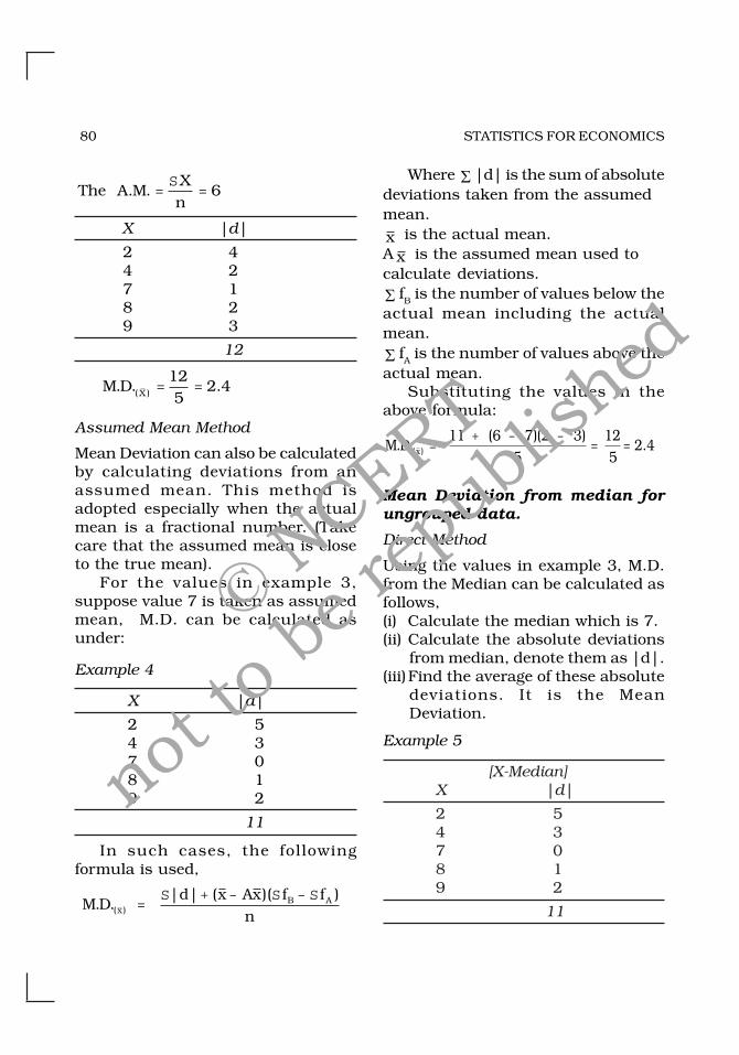
The A MXn

. . = =S

6

X |d|

2 44 27 18 29 3

12

M D X. . .( ) = =125

2 4

Assumed Mean Method

Mean Deviation can also be calculatedby calculating deviations from anassumed mean. This method isadopted especially when the actualmean is a fractional number. (Takecare that the assumed mean is closeto the true mean).

For the values in example 3,suppose value 7 is taken as assumedmean, M.D. can be calculated asunder:

Example 4

X |d|

2 54 37 08 19 2

11

In such cases, the followingformula is used,

M Dd x Ax f f

nxB A. .

| | ( )( )( ) =

+ - -S S S

Where Σ |d| is the sum of absolutedeviations taken from the assumedmean.

x is the actual mean.A x is the assumed mean used tocalculate deviations.

Σ fB is the number of values below theactual mean including the actualmean.

Σ fA is the number of values above theactual mean.

Substituting the values in theabove formula:

M D x. .( )( )

.( ) =+ - -

= = 11 6 7 2 3

5125

2 4

Mean Deviation from median forungrouped data.

Direct Method

Using the values in example 3, M.D.from the Median can be calculated asfollows,(i) Calculate the median which is 7.(ii) Calculate the absolute deviations

from median, denote them as |d|.(iii)Find the average of these absolute

deviations. It is the MeanDeviation.

Example 5

[X-Median]X |d|

2 54 37 08 19 2

11

© NCERT

not to

be re

publi

shed


M. D. from Median is thus,

M Dd

nmedian. .| |

.( ) = = =S 11

52 2

Short-cut method

To calculate Mean Deviation by shortcut method a value (A) is used tocalculate the deviations and thefollowing formula is applied.

M D

d Median A f fn

Median

B A

. .

| | ( )( )( )

=+ - -S S S

where, A = the constant from whichdeviations are calculated. (Othernotations are the same as given in theassumed mean method).

Mean Deviation from Mean forContinuous distribution

TABLE 6.2

Profits of Number ofcompanies Companies(Rs in lakhs) frequenciesClass-intervals

10–20 520–30 830–50 1650–70 870–80 3

40

Steps:

(i) Calculate the mean of thedistribution.

(ii) Calculate the absolute deviations|d| of the class midpoints from themean.

(iii)Multiply each |d| value with itscorresponding frequency to getf|d| values. Sum them up to get

Σ f|d|.

(iv) Apply the following formula,

M Df d

fx. .

| |( )

=S

S

Mean Deviation of the distributionin Table 6.2 can be calculated asfollows:

Example 6

C.I. f m.p. |d| f|d|

10–20 5 15 25.5 127.520–30 8 25 15.5 124.030–50 16 40 0.5 8.050–70 8 60 19.5 156.070–80 3 75 34.5 103.5

40 519.0

M Df d

fx. .

| |.

( )= = =

S

S

51940

12 975

Mean Deviation from Median

TABLE 6.3

Class intervals Frequencies

20–30 530–40 1040–60 2060–80 980–90 6

50

The procedure to calculate MeanDeviation from the median is thesame as it is in case of M.D. fromMean, except that deviations are tobe taken from the median as givenbelow:

© NCERT

not to

be re

publi

shed


Example 7

C.I. f m.p. |d| f|d|

20–30 5 25 25 12530–40 10 35 15 15040–60 20 50 0 060–80 9 70 20 18080–90 6 85 35 210

50 665

M Df d

fMedian. .| |

( ) =S

S

= =66550

13 3.

Mean Deviation: CommentsMean Deviation is based on allvalues. A change in even one valuewill affect it. It is the least whencalculated from the median i.e., itwill be higher if calculated from themean. However it ignores the signsof deviations and cannot becalculated for open-ended distribu-tions.

Standard Deviation

Standard Deviation is the positivesquare root of the mean of squareddeviations from mean. So if there arefive values x1, x2, x3, x4 and x5, firsttheir mean is calculated. Thendeviations of the values from mean arecalculated. These deviations are thensquared. The mean of these squareddeviations is the variance. Positivesquare root of the variance is thestandard deviation.(Note that Standard Deviation iscalculated on the basis of the meanonly).

Calculation of Standard Deviationfor ungrouped data

Four alternative methods are availablefor the calculation of standarddeviation of individual values. Allthese methods result in the samevalue of standard deviation. These are:

(i) Actual Mean Method(ii) Assumed Mean Method(iii)Direct Method(iv) Step-Deviation Method

Actual Mean Method:

Suppose you have to calculate thestandard deviation of the followingvalues:

5, 10, 25, 30, 50

Example 8

X d d2

5 –19 36110 –14 19625 +1 130 +6 3650 +26 676

0 1270

Following formula is used:

s =Sdn

2

s = = =1270

5254 15 937.

Do you notice the value from whichdeviations have been calculated in theabove example? Is it the Actual Mean?

Assumed Mean Method

For the same values, deviations maybe calculated from any arbitrary value

© NCERT

not to

be re

publi

shed


A x such that d = X – A x . Taking A x= 25, the computation of the standarddeviation is shown below:

Example 9

X d d2

5 –20 40010 –15 22525 0 030 +5 2550 +25 625

–5 1275

Formula for Standard Deviation

s = -�

Ł��

�

ł��

S Sdn

dn

2 2

s = --�

Ł��

�

ł�� = =

12755

55

254 15 9372

.

The sum of deviations from a valueother than actul mean is not equalto zero

Direct Method

Standard Deviation can also becalculated from the values directly,i.e., without taking deviations, asshown below:

Example 10

X x2

5 2510 10025 62530 90050 2500

120 4150

(This amounts to taking deviationsfrom zero)

Following formula is used.

s = -Sxn

x2

2( )

or s = -4150

524 2( )

or s = =254 15 937.

Standard Deviation is not affectedby the value of the constant fromwhich deviations are calculated. Thevalue of the constant does not figurein the standard deviation formula.Thus, Standard Deviation isIndependent of Origin.

Step-deviation Method

If the values are divisible by a commonfactor, they can be so divided andstandard deviation can be calculatedfrom the resultant values as follows:

Example 11

Since all the five values are divisibleby a common factor 5, we divide andget the following values:

x x' d d2

5 1 –3.8 14.4410 2 –2.8 7.8425 5 +0.2 0.0430 6 +1.2 1.4450 10 +5.2 27.04

0 50.80

(Steps in the calculation are sameas in actual mean method).

The following formula is used tocalculate standard deviation:

© NCERT

not to

be re

publi

shed


s = ·Sdn

c2

xxc

’ =

c = common factorSubstituting the values,

s = 50.80

5 5

s = ·10 16 5.

s = 15 937.

Alternatively, instead of dividingthe values by a common factor, thedeviations can be divided by acommon factor. Standard Deviationcan be calculated as shown below:

Example 12

x d d' d2

5 –20 –4 1610 –15 –3 925 0 0 030 +5 +1 150 +25 +5 25

–1 51

Deviations have been calculatedfrom an arbitrary value 25. Commonfactor of 5 has been used to dividedeviations.

s =S Sd

ndn

c’ ’2 2

�Ł�

�ł�

·

s = --51

51

55

2�Ł�

�ł�

·

s = =10 16 5 15 937. .·

Standard Deviation is notindependent of scale. Thus, if thevalues or deviations are divided bya common factor, the value of thecommon factor is used in theformula to get the value of StandardDeviation.

Standard Deviation in Continuousfrequency distribution:

Like ungrouped data, S.D. can becalculated for grouped data by any ofthe following methods:(i) Actual Mean Method(ii) Assumed Mean Method(iii)Step-Deviation Method

Actual Mean Method

For the values in Table 6.2, StandardDeviation can be calculated as follows:

Example 13

(1) (2) (3) (4) (5) (6) (7)CI f m fm d fd fd2

10–20 5 15 75 –25.5 –127.5 3251.2520–30 8 25 200 –15.5 –124.0 1922.0030–50 16 40 640 –0.5 –8.0 4.0050–70 8 60 480 +19.5 +156.0 3042.0070–80 3 75 225 +34.5 +103.5 3570.75

40 1620 0 11790.00

Following steps are required:1. Calculate the mean of the

distribution.

xfmf

= = =S

S

162040

40 5.

2. Calculate deviations of mid-valuesfrom the mean so that

d m x= - (Col. 5)3. Multiply the deviations with their

© NCERT

not to

be re

publi

shed


corresponding frequencies to get‘fd’ values (col. 6) [Note that Σ fd= 0]

4. Calculate ‘fd2’ values bymultiplying ‘fd’ values with ‘d’values. (Col. 7). Sum up these toget Σ fd2.

5. Apply the formula as under:

s = = =Sfd

n

2 1179040

17 168.

Assumed Mean Method

For the values in example 13,standard deviation can be calculatedby taking deviations from an assumedmean (say 40) as follows:

Example 14

(1) (2) (3) (4) (5) (6)CI f m d fd fd2

10–20 5 15 -25 –125 312520–30 8 25 -15 –120 180030–50 16 40 0 0 050–70 8 60 +20 160 320070–80 3 75 +35 105 3675

40 +20 11800

The following steps are required:1. Calculate mid-points of classes

(Col. 3)2. Calculate deviations of mid-points

from an assumed mean such thatd = m – A x (Col. 4). AssumedMean = 40.

3. Multiply values of ‘d’ withcorresponding frequencies to get‘fd’ values (Col. 5). (note that thetotal of this column is not zerosince deviations have been takenfrom assumed mean).

4. Multiply ‘fd’ values (Col. 5) with ‘d’values (col. 4) to get fd2 values (col.6). Find Σ fd2.

5. Standard Deviation can becalculated by the followingformula.

s = -�Ł�

�ł�

S Sfdn

fdn

2 2

or s = -�Ł�

�ł�

1180040

2040

2

or s = =294 75 17 168. .

Step-deviation Method

In case the values of deviations aredivisible by a common factor, thecalculations can be simplified by thestep-deviation method as in thefollowing example.

Example 15

(1) (2) (3) (4) (5) (6) (7)CI f m d d' fd' fd'2

10–20 5 15 –25 –5 –25 12520–30 8 25 –15 –3 –24 7230–50 16 40 0 0 0 050–70 8 60 +20 +4 +32 12870–80 3 75 +35 +7 +21 147

40 +4 472

Steps required:

1. Calculate class mid-points (Col. 3)and deviations from an arbitrarilychosen value, just like in theassumed mean method. In thisexample, deviations have beentaken from the value 40. (Col. 4)

2. Divide the deviations by a commonfactor denoted as ‘C’. C = 5 in the

© NCERT

not to

be re

publi

shed


above example. The values soobtained are ‘d'’ values (Col. 5).

3. Multiply ‘d'’ values withcorresponding ‘f'’ values (Col. 2) toobtain ‘fd'’ values (Col. 6).

4. Multiply ‘fd'’ values with ‘d'’ valuesto get ‘fd'2’ values (Col. 7)

5. Sum up values in Col. 6 and Col.7 to get Σ fd' and Σ fd'2 values.

6. Apply the following formula.

s =¢

-¢�

Ł��ł�

·S

S

S

S

fdf

fdf

c2 2

or s = -�Ł�

�ł�

·47240

440

52

or s = - ·11 8 01 5. .

ors

s

= ·

=

11 79 5

17 168

.

.

Standard Deviation: Comments

Standard Deviation, the most widelyused measure of dispersion, is basedon all values. Therefore a change ineven one value affects the value ofstandard deviation. It is independentof origin but not of scale. It is alsouseful in certain advanced statisticalproblems.

5. ABSOLUTE AND RELATIVE MEASURES

OF DISPERSION

All the measures, described so far, areabsolute measures of dispersion. Theycalculate a value which, at times, isdifficult to interpret. For example,consider the following two data sets:

Set A 500 700 1000Set B 100000 120000 130000

Suppose the values in Set A arethe daily sales recorded by an ice-cream vendor, while Set B has thedaily sales of a big departmental store.Range for Set A is 500 whereas for SetB, it is 30,000. The value of Range ismuch higher in Set B. Can you saythat the variation in sales is higherfor the departmental store? It can beeasily observed that the highest valuein Set A is double the smallest value,whereas for the Set B, it is only 30%higher. Thus absolute measures maygive misleading ideas about the extentof variation specially when theaverages differ significantly.

Another weakness of absolutemeasures is that they give the answerin the units in which original valuesare expressed. Consequently, if thevalues are expressed in kilometers, thedispersion will also be in kilometers.However, if the same values areexpressed in meters, an absolutemeasure will give the answer in metersand the value of dispersion will appearto be 1000 times.

To overcome these problems,relative measures of dispersion can beused. Each absolute measure has arelative counterpart. Thus, for Range,there is Coefficient of Range which iscalculated as follows:

Coefficient of Range =-

+

L SL S

where L = Largest valueS = Smallest value

Similarly, for Quartile Deviation, it

© NCERT

not to

be re

publi

shed


be compared even across differentgroups having different units ofmeasurement.

7. LORENZ CURVE

The measures of dispersiondiscussed so far give a numericalvalue of dispersion. A graphicalmeasure called Lorenz Curve isavailable for estimating dispersion.You may have heard of statements like‘top 10% of the people of a countryearn 50% of the national income whiletop 20% account for 80%’. An ideaabout income disparities is given bysuch figures. Lorenz Curve uses theinformation expressed in a cumulativemanner to indicate the degree ofvariability. It is specially useful incomparing the variability of two ormore distributions.

Given below are the monthlyincomes of employees of a company.

TABLE 6.4

Incomes Number of employees

0–5,000 55,000–10,000 1010,000–20,000 1820,000–40,000 1040,000–50,000 7

is Coefficient of Quartile Deviationwhich can be calculated as follows:

Coefficient of Quartile Deviation

=-

+

Q QQ Q

3

3

1

1 where Q3=3rd Quartile

Q1 = 1st QuartileFor Mean Deviation, it is

Coefficient of Mean Deviation.Coefficient of Mean Deviation =

M D x

xor

M D MedianMedian

. .( ) . .( )

Thus if Mean Deviation iscalculated on the basis of the Mean,it is divided by the Mean. If Median isused to calculate Mean Deviation, itis divided by the Median.

For Standard Deviation, therelative measure is called Coefficientof Variation, calculated as below:

Coefficient of Variation

= Standard Deviation

Arithmetic Mean· 100

It is usually expressed inpercentage terms and is the mostcommonly used relative measure ofdispersion. Since relative measuresare free from the units in which thevalues have been expressed, they can

Example 16

Income Mid-points Cumulative Cumulative No. of Comulative Comulativelimits mid-points mid-points as employees frequencies frequencies as

percentages frequencies percentages(1) (2) (3) (4) (5) (6) (7)

0–5000 2500 2500 2.5 5 5 105000–10000 7500 10000 10.0 10 15 3010000–20000 15000 25000 25.0 18 33 6620000–40000 30000 55000 55.0 10 43 8640000–50000 45000 100000 100.0 7 50 100

© NCERT

not to

be re

publi

shed


Construction of the Lorenz Curve

Following steps are required.

1. Calculate class mid-points andfind cumulative totals as in Col. 3in the example 16, given above.

2. Calculate cumulative frequenciesas in Col. 6.

3. Express the grand totals of Col. 3and 6 as 100, and convert thecumulative totals in these columnsinto percentages, as in Col. 4 and 7.

4. Now, on the graph paper, take thecumulative percentages of thevariable (incomes) on Y axis andcumulative percentages offrequencies (number of employees)on X-axis, as in figure 6.1. Thuseach axis will have values from ‘0’to ‘100’.

5. Draw a line joining Co-ordinate(0, 0) with (100,100). This is calledthe line of equal distributionshown as line ‘OC’ in figure 6.1.

6. Plot the cumulative percentages ofthe variable with correspondingcumulative percentages offrequency. Join these points to getthe curve OAC.

Studying the Lorenz Curve

OC is called the line of equaldistribution, since it would imply asituation like, top 20% people earn20% of total income and top 60% earn60% of the total income. The fartherthe curve OAC from this line, thegreater is the variability present in thedistribution. If there are two or morecurves, the one which is the farthest

from line OC has the highestdispersion.

8. CONCLUSION

Although Range is the simplest tocalculate and understand, it is undulyaffected by extreme values. QD is notaffected by extreme values as it isbased on only middle 50% of the data.However, it is more dif ficult tointerpret M.D. and S.D. both are basedupon deviations of values from theiraverage. M.D. calculates average ofdeviations from the average butignores signs of deviations andtherefore appears to be unmathema-tical. Standard Deviation attempts tocalculate average deviation frommean. Like M.D., it is based on allvalues and is also applied in moreadvanced statistical problems. It isthe most widely used measure ofdispersion.

© NCERT

not to

be re

publi

shed


EXERCISES

1. A measure of dispersion is a good supplement to the central value inunderstanding a frequency distribution. Comment.

2. Which measure of dispersion is the best and how?

3. Some measures of dispersion depend upon the spread of values whereassome calculate the variation of values from a central value. Do you agree?

4. In a town, 25% of the persons earned more than Rs 45,000 whereas 75%earned more than 18,000. Calculate the absolute and relative values ofdispersion.

5. The yield of wheat and rice per acre for 10 districts of a state is as under:District 1 2 3 4 5 6 7 8 9 10Wheat 12 10 15 19 21 16 18 9 25 10Rice 22 29 12 23 18 15 12 34 18 12Calculate for each crop,(i) Range(ii) Q.D.(iii) Mean Deviation about Mean(iv) Mean Deviation about Median(v) Standard Deviation(vi) Which crop has greater variation?(vii)Compare the values of different measures for each crop.

6. In the previous question, calculate the relative measures of variation andindicate the value which, in your opinion, is more reliable.

7. A batsman is to be selected for a cricket team. The choice is between Xand Y on the basis of their five previous scores which are:

Recap

• A measure of dispersion improves our understanding about thebehaviour of an economic variable.

• Range and Quartile Deviation are based upon the spread of values.• M.D. and S.D. are based upon deviations of values from the average.• Measures of dispersion could be Absolute or Relative.• Absolute measures give the answer in the units in which data are

expressed.• Relative smeasures are free from these units, and consequently can

be used to compare different variables.• A graphic method, which estimates the dispersion from shape

of a curve, is called Lorenz Curve.

© NCERT

not to

be re

publi

shed


X 25 85 40 80 120Y 50 70 65 45 80Which batsman should be selected if we want, (i) a higher run getter, or(ii) a more reliable batsman in the team?

8. To check the quality of two brands of lightbulbs, their life in burninghours was estimated as under for 100 bulbs of each brand.

Life No. of bulbs(in hrs) Brand A Brand B

0–50 15 250–100 20 8100–150 18 60150–200 25 25200–250 22 5

100 100

(i) Which brand gives higher life?(ii) Which brand is more dependable?

9. Averge daily wage of 50 workers of a factory was Rs 200 with a StandardDeviation of Rs 40. Each worker is given a raise of Rs 20. What is thenew average daily wage and standard deviation? Have the wages becomemore or less uniform?

10. If in the previous question, each worker is given a hike of 10 % in wages,how are the Mean and Standard Deviation values affected?

11. Calculate the Mean Deviation about Mean and Standard Deviation for thefollowing distribution.

Classes Frequencies

20–40 340–80 680–100 20100–120 12120–140 9

50

12. The sum of 10 values is 100 and the sum of their squares is 1090. Findthe Coefficient of Variation.

© NCERT

not to

be re

publi

shed

measures of dispersion - evirtualguruevirtualguru.com/books/ncert/11class/statistics... · ·...

Documents