measurements of the static and dynamic load …
TRANSCRIPT
MEASUREMENTS OF THE STATIC AND DYNAMIC LOAD
PERFORMANCE OF A WATER LUBRICATED HYBRID THRUST
BEARING
A Thesis
by
MICHAEL S. WILKINSON
Submitted to the Office of Graduate Studies of Texas A&M University
in partial fulfillment of the requirements for the degree of
MASTER OF SCIENCE
Chair of Committee, Luis San Andrés Committee Members, Adolfo Delgado Theofanis Strouboulis Head of Department, Andreas Polycarpou
May 2019
Major Subject: Mechanical Engineering
Copyright 2019 Michael Scott Wilkinson

ii
ABSTRACT
After a successful static load testing campaign in 2015, the thrust bearing test rig has
been reconfigured for dynamic load tests to determine force coefficients (stiffness,
damping, and added mass). Continuous lubrication flow is supplied by a new, closed-
loop water supply system capable of a wide range of operating conditions and long
duration testing with little waste. In addition, a fully-instrumented loading system
enables simultaneous static and dynamic (impact) loading. Cumulatively, these changes
enable reliable dynamic load testing while maintaining full static load test functionality.
The test rig is equipped to produce experimental results to validate bearing force
coefficient model predictions.
Static force vs. displacement measurements are taken to validate test rig performance
after modification to accommodate the new loading and water supply systems. Overall
static load results match well with predictions as well as prior experimental results.
Axial clearance (C0) increases as the TTB lubrication pressure (Ps) increases. With a
constant supply pressure (Ps), however, the test TB axial clearance (C0) decreases as the
applied axial load (W/A) increases. Large uncertainties, due in part to the allowable run
out of the thrust collar (±10µm), continue to plague axial displacement measurements.
Dynamic load tests are then performed for moderate shaft speed (up to 6krpm) and
quantified with force coefficients derived from the system complex dynamic stiffness
function. Measurements indicate that the test thrust bearing shows no appreciable change
in dynamic force coefficients (axial stiffness, damping and inertia) for the range of rotor
speeds examined herein. This behavior proves the bearing behaves in a mainly
iii
hydrostatic mode as it lacks hydrodynamic features that capitalize on bearing surface
speed for performance. In contrast, with an increase in applied static load at constant
supply pressure the test bearing stiffness and damping increase while added mass does
not show appreciable change. Finally, an increase in supply pressure under constant
applied load yields an increase in stiffness and damping coefficients with no change to
added mass. As with static load measurements, inherent uncertainty associated clearance
measurements are large and combine with an additional error due to repeatability of the
impact tests.
A recommendation for future work is to fabricate a new rotor with tighter tolerances
for the critical run out dimension. Lower run out tolerance will greatly reduce the
clearance uncertainty, instilling better confidence in both static and dynamic
experimental results.
iv
DEDICATION
I thank Dr. San Andrés for the opportunity to work and learn at the Turbomachinery
Laboratory. Additionally, I thank the Turbomachinery Research Consortium for their
financial support. I thank Mr. Michael Rohmer, Mr. Hardik Jani, Mr. Hameed Haq, Mr.
Giovanni Palini, Mr. Travis Cable, Ms. Avery Carnahan, Ms. Casey Yowell, Mr. Blake
Bontz, Mr. Juan Francisco Ordonez and other colleagues at the Turbomachinery
Laboratory for their support. Finally, thanks to my family for their encouragement.

v
CONTRIBUTORS AND FUNDING SOURCES
This work was supervised by a thesis (or) dissertation committee consisting of
Professor(s) San Andrés [advisor] and Delgado of the Department of Mechanical
Engineering and Professor Strouboulis of the Department of Aerospace Engineering. All
work for the thesis (or) dissertation was completed by the student, under the advisement
of Professor San Andrés of the Department of Mechanical Engineering.
This work was made possible in part by funding from the Turbomachinery
Research Consortium, and the Turbomachinery Laboratory at Texas A&M University.

vi
NOMENCLATURE
1-DOF One degree of freedom
A Thrust bearing area [m2]
C0 Axial clearance between thrust bearing center and thrust collar [μm ]
CTTB Thrust bearing damping coefficient [ Ns m]
FCable Force exerted by taut cable [N]
Fd Applied dynamic (impact) load [N]
FFT Fast Fourier Transform
FTTB Thrust bearing reaction force [N]
H Dynamic (complex) stiffness of thrust bearing
= HR + i HI
HTB Hybrid Thrust Bearing (hydrostatic plus hydrodynamic)
i Imaginary unit, 1i
KCable Taut cable stiffness [ N m] = 93.15 kN/m
KTTB Thrust bearing stiffness coefficient [ N m]
M Mass of thrust bearing, load shaft and load cell [kg]
MTTB Thrust bearing added mass coefficient [ 2Ns m ]
N Number of impacts for average
PJ
PT
Journal bearing supply pressure [bar(g)]
Thrust bearing supply pressure [bar(g)]
Rout Thrust collar outer radius [cm]

vii
SSV Subsynchronous speed vibration
TTB Test Thrust Bearing
VI Visual Interface
VFD Variable Frequency Drive
z Relative displacement between rotor and test thrust bearing [μm ]
Rz Absolute axial displacement of rotor [μm ]
TTBz Absolute displacement of test thrust bearing [μm ]
Ω Rotor speed [rad/s]
ω Excitation frequency [rad/s]
W/A Specific Load [bar]

viii
TABLE OF CONTENTS
Page
ABSTRACT .................................................................................................................................... ii
DEDICATION ............................................................................................................................... iv
CONTRIBUTORS AND FUNDING SOURCES ........................................................................... v
NOMENCLATURE ....................................................................................................................... vi
TABLE OF CONTENTS ............................................................................................................. viii
LIST OF TABLES .......................................................................................................................... x
LIST OF FIGURES ........................................................................................................................ xi
INTRODUCTION ........................................................................................................................... 1
TEST RIG DESCRIPTION ............................................................................................................ 2
LITERATURE REVIEW ................................................................................................................ 8
Background ................................................................................................................................. 8
Principle of Operation of a Hybrid Bearing ................................................................................ 8
High Performance Thrust Bearings for High Rotor Speed Applications .................................... 9
Parameter Identification Methods ............................................................................................. 10
Previous Work ........................................................................................................................... 11
TEST RIG MODIFICATIONS ..................................................................................................... 16
Water Supply System ................................................................................................................ 16
Dynamic Load Mechanism ....................................................................................................... 19
SYSTEM MODEL FOR PARAMETER IDENTIFICATION ..................................................... 28
ix
DATA ACQUISITION AND PROCESSING .............................................................................. 32
Data Acquisition ........................................................................................................................ 32
Data Processing ......................................................................................................................... 33
THRUST BEARING PERFORMANCE ...................................................................................... 36
STATIC LOAD PERFORMANCE .............................................................................................. 37
Static Load Tests at Various Supply Pressures and Rotor Speeds ............................................ 38
Static Load Tests at Various Rotor Speeds ............................................................................... 41
DYNAMIC LOAD PERFORMANCE ......................................................................................... 45
Dynamic Load Tests at Various Supply Pressures and a Fixed Rotor Speed ........................... 46
Dynamic Load Tests at Various Rotor Speeds and a Fixed Supply Pressure ........................... 50
CONCLUSION ............................................................................................................................. 54
REFERENCES .............................................................................................................................. 56
APPENDIX A INSTRUMENTATION ........................................................................................ 59
APPENDIX B ROTOR THRUST COLLAR PLANE EQUATION DERIVATION .................. 60
APPENDIX C UNCERTAINTY ANALYSIS ............................................................................. 63
Static Load Measurements ........................................................................................................ 63
Dynamic Load Measurements ................................................................................................... 64
APPENDIX D DETERMINATION OF CABLE STIFFNESS .................................................... 66

x
LIST OF TABLES
Page
Table 1. Test Matrix for static load tests at null to moderate shaft speed. .................................... 38
Table 2. Test Matrix for dynamic load tests for operation at various TTB supply pressure
and applied static load conditions. .................................................................................... 45
Table 3. Test Matrix for dynamic load tests for operation at null to moderate
shaft speeds. ...................................................................................................................... 46
Table 4. Instrumentation utilized for TTB dynamic load testing .................................................. 59
Table 5. Horizontal and vertical positions of each eddy current sensor relative to
the center of the thrust bearing. ......................................................................................... 61
xi
LIST OF FIGURES
Page
Figure 1. Photograph of test rig (2015) ........................................................................................... 4
Figure 2. Cross sectional view of the thrust bearing test rig [1]. .................................................... 5
Figure 3. Photograph [4] and physical parameters of hybrid (hydrostatic/ hydrodynamic)
thrust bearing ....................................................................................................................... 5
Figure 4. Photograph of rotor [15] .................................................................................................. 6
Figure 5. Schematic view of the flexure pivot, tilting pad hydrostatic journal bearing. [3] ........... 6
Figure 6. Schematic View of Test Rig: Thrust and Journal Bearings Represented as
Mechanical Elements with Stiffness and Damping Coefficients [4] .................................. 7
Figure 7. Schematic view of closed loop water supply system for thrust bearing test rig. ........... 18
Figure 8. Photograph depicting major components of the water supply system. .......................... 19
Figure 9. Schematic diagram of an early axial loading mechanism. ............................................. 21
Figure 10. Impact load test to determine resonant frequency of a strain gauge load cell. ............ 23
Figure 11. Dynamic signal analyzer output of strain gauge load cell impact test showing
a resonant frequency at 1728 Hz with good coherence between the delivered impact load (input) and the measured acceleration (output). ............................................ 22
Figure 12. Schematic of redesigned, cable-loaded loading system and the geometry of
the taut cable used to derive the equivalent static load along the axial direction, Fr. ...................................................................................................................................... 25
Figure 13. Photograph of taut cable load mechanism. .................................................................. 26
xii
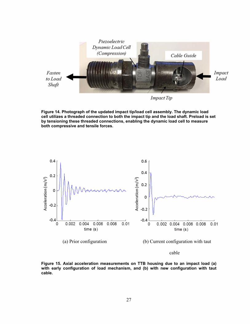
Figure 14. Photograph of the updated impact tip/load cell assembly. The dynamic load
cell utilizes a threaded connection to both the impact tip and the load shaft. Preload is set by tensioning these threaded connections, enabling the dynamic load cell to measure both compressive and tensile forces. ................................................ 27
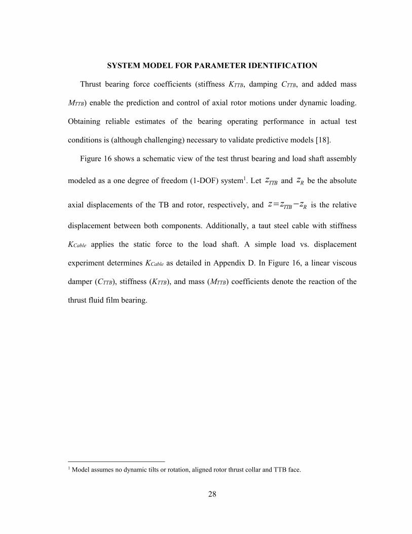
Figure 15. Axial acceleration measurements on TTB housing due to an impact
load (a) with early configuration of load mechanism, and (b) with new configuration with taut cable. ............................................................................................ 27
Figure 16. Schematic view of 1-DOF model of test TB for parameter identification. ................. 29
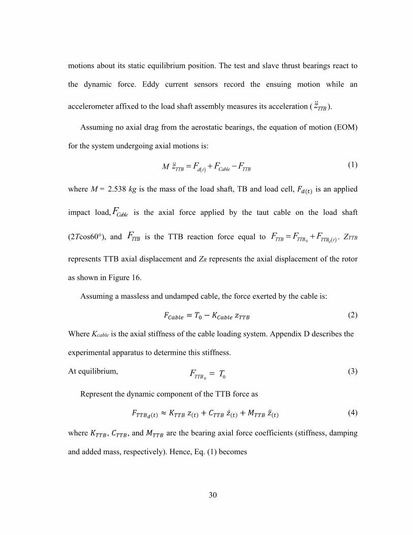
Figure 17. Visual Interface (VI) front panel recording dynamic impact test data. ....................... 33
Figure 18. Sample linear curve fit of the (a) real and (b) imaginary portions of the TTB
complex stiffness (H) vs frequency. W/A is the specific load defined as the axial load per unit area. Note that A = 32.6 cm2 ........................................................................ 35
Figure 19. Axial clearance (C0) versus specific load (W/A) for operation at four
TTB supply pressures (Ps) and rotor speed at 3 krpm. Horizontal error bars represent the uncertainty in the axial load at a 95% confidence interval. Vertical error bars indicate the uncertainty in the axial clearance due to the machined runout of the rotor ............................................................................................................. 35
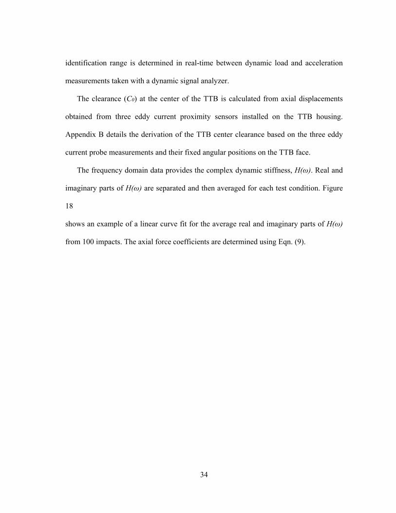
Figure 20. Axial clearance (C0) versus specific load (W/A) for operation at four
TTB supply pressures (Ps) and rotor speed at 4 krpm. Horizontal error bars represent the uncertainty in the axial load at a 95% confidence interval. Vertical error bars indicate the uncertainty in the axial clearance due to the machined runout of the rotor. ............................................................................................................ 40
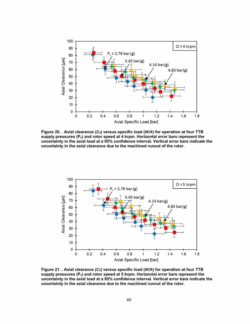
Figure 21. Axial clearance (C0) versus specific load (W/A) for operation at four
TTB supply pressures (Ps) and rotor speed at 5 krpm. Horizontal error bars represent the uncertainty in the axial load at a 95% confidence interval. Vertical error bars indicate the uncertainty in the axial clearance due to the machined runout of the rotor. ............................................................................................................ 40
xiii
Figure 22. Axial clearance (C0) versus specific load (W/A) for operation at four
TTB supply pressures (Ps) and rotor speed at 6 krpm. Horizontal error bars represent the uncertainty in the axial load at a 95% confidence interval. Vertical error bars indicate the uncertainty in the axial clearance due to the machined runout of the rotor. ............................................................................................................ 35
Figure 23. Axial clearance (C0) versus specific load (W/A) for operation at various rotor
speeds for operation with supply pressure Ps = 2.76 bar(g). Horizontal error bars represent the uncertainty in the axial load at a 95% confidence interval. Vertical error bars indicate the uncertainty in the axial clearance due to the machined runout of the rotor. ............................................................................................................ 42
Figure 24. Axial clearance (C0) versus specific load (W/A) for operation at various rotor
speeds for operation with supply pressure PS = 3.45 bar(g). Horizontal error bars represent the uncertainty in the axial load at a 95% confidence interval. Vertical error bars indicate the uncertainty in the axial clearance due to the machined runout of the rotor. ............................................................................................................ 42
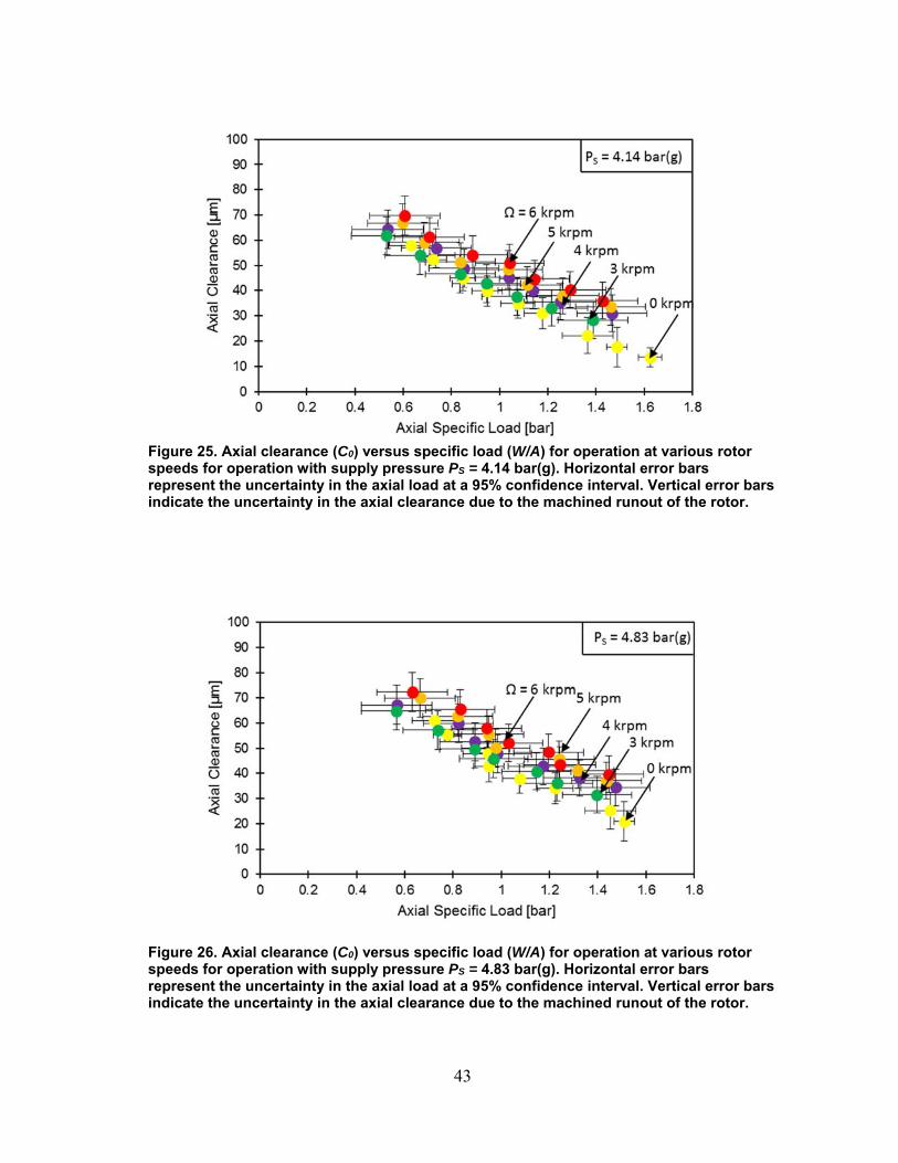
Figure 25. Axial clearance (C0) versus specific load (W/A) for operation at various rotor
speeds for operation with supply pressure PS = 4.14 bar(g). Horizontal error bars represent the uncertainty in the axial load at a 95% confidence interval. Vertical error bars indicate the uncertainty in the axial clearance due to the machined runout of the rotor. ............................................................................................................ 43
Figure 26. Axial clearance (C0) versus specific load (W/A) for operation at various rotor
speeds for operation with supply pressure PS = 4.83 bar(g). Horizontal error bars represent the uncertainty in the axial load at a 95% confidence interval. Vertical error bars indicate the uncertainty in the axial clearance due to the machined runout of the rotor. ............................................................................................................ 43
Figure 27. Experimentally measured and predicted axial stiffness coefficient (Kz) for
TTB operating with water supplied at 2.75, 3.45 and 4.14 bar(g) and shaft speed of 3 krpm. Applied specific axial load, W/A = 0.49 bar, 0.61 bar, and 0.73 bar. ............. 48

xiv
Figure 28. Measured and predicted damping coefficient (Cz) for TTB operating
with water supplied at 2.75, 3.45 and 4.14 bar and shaft speed of 3 krpm. Applied specific axial load, W/A = 0.49 bar, 0.61 bar, and 0.73 bar. ............................................. 49
Figure 29. Measured and predicted added mass coefficient (Mz) for TTB operating with
water supplied at 2.75, 3.44 and 4.13 bar and shaft rotational speed of 3 krpm. Applied specific axial loads of 0.49 bar, 0.61 bar, and 0.73 bar. ...................................... 50
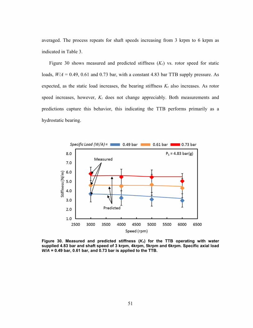
Figure 30. Measured and predicted stiffness (Kz) for the TTB operating with
water supplied 4.83 bar and shaft speed of 3 krpm, 4krpm, 5krpm and 6krpm. Specific axial load W/A = 0.49 bar, 0.61 bar, and 0.73 bar is applied to the TTB. .......... 51
Figure 31. Measured and predicted damping (Cz) for the TTB operating with
water supplied at 4.83 bar psi(g) and shaft speed of 3 krpm, 4krpm, 5krpm and 6krpm. Specific axial load W/A = 0.49 bar, 0.61 bar, and 0.73 bar is applied to the TTB. ............................................................................................................................ 52
Figure 32. Measured and predicted added mass (Mz) for the TTB operating with water
supplied at 4.83 bar psi(g) and shaft speed of 3 krpm, 4krpm, 5krpm and 6krpm. Specific axial load W/A = 0.49 bar, 0.61 bar, and 0.73 bar is applied to the TTB. .......... 53
Figure 33: Reference diagram of a thrust bearing for geometric calculation of clearance
as a function of displacements recorded at T1, T2, and T3............................................... 60
Figure 34. Averaged displacement response for four series of 25 impacts performed for
operation at a rotor speed of 3krpm, thrust bearing supply pressure of 3.45 bar(g) ......... 65
Figure 35. Schematic of an ad-hoc setup used to record the axial stiffness of a
static loading mechanism. ................................................................................................. 67
Figure 36. Applied force vs. displacement results for determination of the axial stiffness
of the static loading mechanism. ....................................................................................... 67

1
INTRODUCTION
In rotating machinery, fluid lubricated thrust bearings maintain axial position and
support axial loads applied to the rotor. The performance and reliability of these
machines depend on adequate axial load support tailored to the operating conditions of
the machine. Prediction of these thrust forces is largely empirical, emphasizing the need
to design and test thrust bearings for use in reliable rotating equipment [1].
Presently, dynamic load tests are performed with a purpose-built test rig on a hybrid
thrust bearing. The thesis results will advance bearing technology by offering
experimental data to compare with predictions generated by a predictive software in Ref.
[2].
In 2015, a water lubricated thrust bearing test rig is revamped after severe damage
was incurred in 2013 due to large amplitude vibrations during operation with air
lubricated radial bearings [1]. Static load tests performed in 2015 [3] paved the way for
the dynamic load testing discussed herein.
This thesis reviews relevant literature pertaining to the project, describes test rig
modifications, overviews system modelling, outlines the data acquisition and processing
methods, and presents test results for dynamic impact load tests. The test rig is presently
used to measure the static and dynamic performance for various thrust bearing and face
seals.

2
TEST RIG DESCRIPTION
Figure 1 shows a photograph and Figure 2 shows a cross section view [4] of an
existing thrust bearing test rig constructed to quantify the static and dynamic load
performance of water lubricated hybrid thrust bearings. Water supplies two flexure-pivot
tilting-pad hydrostatic journal bearings to enable the lateral support of the rotor. Two
water-lubricated hybrid (hydrostatic and hydrodynamic) thrust bearings, test and slave,
control the axial position of the rotor.
Figure 3 depicts a photograph of the test hybrid (hydrostatic plus hydrodynamic)
thrust bearing (HTB) [4]. With sufficiently small clearances between the HTB and the
rotor thrust collar (see Figure 4), load support is generated by restricting water flow
through eight orifices to pressurize the eight corresponding recessed areas. An identical,
albeit with slightly larger orifices, smaller pockets and split in half for ease of
installation, slave thrust bearing counteracts the load generated by the test thrust bearing.
Both HTBs are manufactured with 660 Bearing Bronze and have inner and outer
diameters of 40.6 mm and 76.2 mm, respectively. Each pocket is 20° in arc length, 8.13
mm in radial length, pocket depths of 0.51 mm (Test) and 0.44 mm (Slave).
Figure 5 shows one of two identical flexure pivot, tilting pad hybrid
(hydrostatic/hydrodynamic) radial bearings supporting the rotor [3]. Electron discharge
machining (EDM) is used to manufacture the flexible pivot, tilting pad bearing out of a
660 Bearing Bronze material. The bearings are fabricated in two pieces, top and bottom
halves, to simplify the installation process. Both the inner diameter and the bearing
length are manufactured to be 3.81 cm for an operating radial clearance of 89 µm. Both

3
bearings have four 72° pads, 20% preload, with 60% pivot offset [5]. The 8.7 lb stainless
steel rotor, shown in Figure 4, has its center of mass midway between two radial
bearings. The rotor consists of opposing test and slave thrust collars and a threaded
connection to interface with the flexible motor coupling.
A loading mechanism moves the test thrust bearing axially and applies the load to
the rotor thrust collar. As shown on the left of Figure 2, two air bearings support the non-
rotating load shaft while allowing the shaft to move axially with minimal friction when a
load is applied. The rotor transmits the load to the slave thrust bearing. The slave bearing
side of the rotor connects to a Variable Frequency Drive (VFD) controlled electric motor
via a flexible coupling.
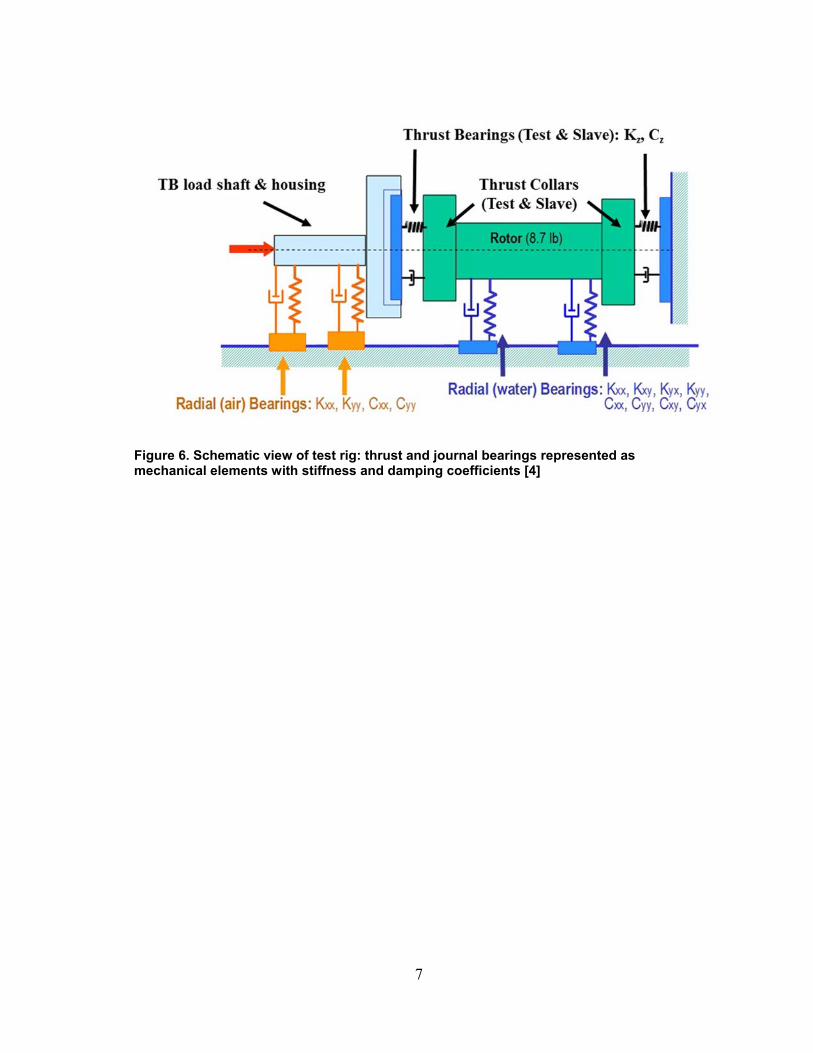
Figure 6 shows a schematic view of the test rig with the thrust bearings and journal
bearings represented as mechanical elements with stiffness and damping characteristics
(radial and axial) [4]. In the system modelling section of this report, the assembly is
represented as a one degree of freedom system for determination of the axial bearing
force coefficients (stiffness, damping, and added mass).

4
Figure 1. Photograph of test rig (2015)

5
Figure 2. Cross sectional view of the thrust bearing test rig [1].
Material: 660 Bearing Bronze
Slave Bearing
Test Bearing
Thrust Face
Inner Diameter, Din 40.64 mm Outer Diameter, Dout 76.2 mm Thrust Bearing Area, A 32.6 cm2
Flange Outer Diameter 98.43 mm
Number of Pockets 8 Arc Length 20° Radial Length 8.13 mm Depth 0.44 mm 0.51 mmPocket/Wetted Area Ratio
0.19
Orifice
Orifices/Pocket 1 Diameter, dorif 1.80 mm 1.55 mm
Figure 3. Photograph [4] and physical parameters of hybrid (hydrostatic/hydrodynamic) thrust bearing

6
Figure 4. Photograph of rotor [15]
Figure 5. Schematic view of the flexure pivot, tilting pad hydrostatic journal bearing. [3]
7
Figure 6. Schematic view of test rig: thrust and journal bearings represented as mechanical elements with stiffness and damping coefficients [4]

8
LITERATURE REVIEW
Background
Hybrid Thrust Bearings (HTBs) exhibit features of both hydrostatic and
hydrodynamic bearings. Where hydrodynamic bearings function with a fluid film
pressure generated from a rotating shaft, hydrostatic bearings provide support without
shaft speed by utilizing an external pressurization system. This ensures no contact of
surfaces at a low or null rotational speed though at the cost of external energy required to
pressurize the bearing. Lubricant supply pressure and shaft rotational speed dictate the
bearing load capacity, drag torque, and axial force coefficients.
Principle of Operation of a Hybrid Bearing
Rowe (1983) [6] details HTB operation with its load support and stiffness generated
as fluid flow passes through a flow restrictor (such as an orifice, a capillary or a constant
flow valve). An additional flow resistance occurs as the fluid flows through a small
clearance or film land region. As this clearance decreases, the flow rate reduces and the
head loss through the orifice also decreases; causing an increase in recess pressure. The
recess pressure does not exceed supply pressure except for cases where shaft speed is
large enough to generate an additional hydrodynamic pressure. Hybrid bearings perform
like hydrostatic bearings at a low rotational shaft speed and exhibit hydrodynamic
behavior with a significantly high shaft speed. An increased recess pressure induces a
higher load on the rotor and increases the gap (clearance) between the rotor and the
bearing. The opposite is true for a decrease in applied load; flow rate and head loss
through the orifice increase, thus causing the recess pressure to decrease. A decrease in
9
recess pressure with a constant applied load induces a smaller clearance between the
rotor and the bearing. Bearing stiffness and damping force coefficients are thus related to
the conditions of the supply flow.
High Performance Thrust Bearings for High Rotor Speed Applications
In cryogenic fluid turbo pump applications fluid film hybrid bearings offer an
alternative to ultra-precision ceramic ball bearings for rotor support [7]. High shaft
speeds utilized by turbo pumps mandate the use of bearings with little or no surface
speed limitation, a feature unique to fluid film hybrid bearings. These bearings allow the
turbopump to be smaller and lighter while operating with an increased mechanical
efficiency.
Using a bulk flow analysis, San Andrés (2000) [8] predicts the performance of a
multi-recess, orifice-compensated, angle injected HTB. For a high pressure cryogenic
density turbo pump example, the study analyzes bearing operation with high shaft speed
(180 krpm) and a high pressure differential (550 bar). The bearing stiffness coefficient is
highest when the recess pressure is 60% of the supply pressure (both relative to ambient
conditions). The bearing damping coefficient increases with a decrease in clearance and
an increase in rotor speed. Centrifugal fluid inertia becomes an issue at a sufficiently
high rotor speed and a low load conditions as it may induce starvation on the bearing
inner side diameter and a suction pressure just downstream of the recess. Including the
effect of fluid inertia across the recesses and the film lands, the damping coefficient is
higher and the stiffness coefficient lower than the analysis considering the recesses
alone, indicating that fluid inertia plays a large role in fluid bearing performance.
10
Safar (1983) [9] analyzes the effect of centrifugal forces on misaligned hydrostatic
thrust bearings. Centrifugal forces cause load capacity and drag torque to reduce
considerably while increasing the flow rate across the bearing. Centrifugal effects
diminish with an increase in collar angular misalignment.
San Andrés (2002) [2] utilizes his computational model to study the effects of
angular misalignment on HTB performance for a cryogenic turbopump operating at a
rotational speed of 180 krpm. Axial and moment-angle stiffness coefficients (both static
and dynamic) peak when the recess pressure ratio is approximately 0.6. Axial damping,
direct moment angle damping and cross-coupled moment angle stiffness coefficients
increase moderately with load for high clearance/low load conditions and then rapidly
with load for low clearance/high load conditions due to the increased hydrodynamic
effect while operating at a low clearance. With an increase in misalignment angle
between the thrust bearing and the rotor, the moment angle and axial stiffness
coefficients increase while axial force and drag torque remain unaffected. Additionally,
an increase in misalignment angle causes an increased differential in pressure across the
recesses and film lands which, in turn, causes a decrease in the mass flow rate through
the inner diameter of the bearing.
Parameter Identification Methods
Parameter identification requires measurement of the rotor displacement (response)
due to a controlled external load excitation [10]. These measurements allow the
estimation of the bearing complex stiffness (or impedance) in the frequency domain
[11]. Periodic force and impact load excitations applied to the thrust bearing are the most

11
feasible means to excite the system. Periodic loads can be exerted through a shaker
attached to the test bearing. Independent adjustment of the shaker frequency allows
studying frequency dependence of the bearing force coefficients [10]. Alternatively, a
transient load excitation of a rotor-bearing system through impact loads has the
advantage of exciting a broad range of excitation frequencies in a single experiment,
thus reducing the time required for testing.
Previous Work
Prior to the current work, former students of Texas A&M University constructed and
performed tests with the above described test rig.
Forsberg (2008) [12] designs and constructs a (non-rotating shaft) thrust bearing test
rig to measure the performance of a water-lubricated, eight pocket HTB operating with
supply pressure ranging from 3.45 bar(g) to 17.24 bar (g). The pocket pressure ratio
(ratio of pocket pressure to supply pressure to the test thrust bearing,
PRatio=Ppocket/Psupply) has a large influence on the operating clearance (load) between the
thrust bearing and thrust collar of the rotor. An increase in pocket pressure, stemming
from either an increase in supply pressure or a decrease in clearance, correlates to an
increase in bearing load capacity and stiffness. Measurements of flow and load capacity
agree within 20% of predictions generated by San Andrés [2], while a static stiffness
approximation demonstrates a large discrepancy from predictions due to misalignment
between the thrust bearing face and the thrust collar of the rotor.
Ramirez (2008) [13] continues Forsberg work with the same water lubricated, 8
pocket HTB with supply pressure ranging from 3.45 bar (g) to 17.24 bar (g) but with an
12
operating shaft speed ranging from 7.5 krpm to 17.5 krpm (ΩR = 69.8/m/s). Shaft speed
is found to have little influence on the load capacity and axial stiffness of the test
bearing. At a high shaft speed and low load, flow rate measurements through the inner
diameter indicate the onset of fluid starvation due to centrifugal fluid flow acceleration.
Inlet flow rate, inner diameter discharge flow rate, load capacity, and recess pressure
ratio measurements agree closely with predictions derived in [2], differing by 1%, 5%,
7%, and 10%, respectively.
Esser (2010) [14] carries on work by Forsberg and Ramirez by determining the effect
of orifice diameter (1.67 mm, 1.80 mm, and 1.93 mm) on the performance of the same
water-lubricated, eight pocket HTB with supply pressure ranging from 3.45 bar (g) to
17.24 bar (g) and shaft speeds ranging from 7.5 krpm to 17.5 krpm. With a constant
applied load and a constant thrust bearing supply pressure, the bearing stiffness and
clearance increase with an increase in feed orifice diameter. Flow rate increases with a
larger orifice diameter, preventing the onset of inner bearing starvation predicted by
Forsberg and Ramirez [12, 13]. A limited increase in bearing axial stiffness occurs when
the orifice diameter changes from 1.80 mm to 1.93 mm, while the flow rate demanded is
significantly higher. Measurements for inlet flow rate, inner diameter discharge flow
rate, recess pressure, clearance, and axial stiffness coefficient agree well with
predictions.
San Andrés et al. (2016) [4] examine the performance of a hydrostatic thrust bearing
subjected to increasing static load (max. 3600 N), shaft speed up to 17.5krpm (ΩR = 70
m/s) and increasing supply pressure (max. 17.2 bar). Predictions generated from a bulk
13
flow model [2], accounting for fluid inertia and turbulent flow effects, agree well with
the experimental results. Measured parameters include flow rates (supply and return
through thrust bearing inner diameter), pocket pressure, and fluid film clearance. As the
applied load increases, predictions and measurements show that the film clearance and
flow rate decrease exponentially. Measurements validate a predicted fluid starvation
event at the highest speed and lowest supply pressure condition. Measured flow rate and
bearing pocket pressure data enable the empirical estimation of the bearing discharge
coefficient for use in the predictive tool.
Rohmer (2016) [15] details a catastrophic failure (occurring in 2013) as well as many
repairs and modifications to the test rig described above. In 2014, the test rig was
modified to host hydrostatic gas (air) bearings. The failure occurred when a high
amplitude subsynchronous speed vibration (SSV) was observed at approximately 28
krpm [1]. After the failure incident, the test rig was converted back to operation with
water. Revamping of the test rig, completed in 2015, includes: manufacturing two new
rotors, repairing the damaged threads on the housing, aligning the motor shaft centerline
and the test rotor centerline, upgrading the water manifold to mitigate pressure losses,
designing a load system capable of static and/or dynamic loads, installing
instrumentation, and developing means of data acquisition. Measurements of the free-
free mode natural frequencies and mode shapes of the rotor-coupling system show that
the test rotor and quill shaft coupling must be considered as a single unit for accurate
rotordynamic analysis.
14
Without rotor speed, Rohmer et al. (2018) [3] measure the static load performance of
a hybrid thrust bearing lubricated with water at room temperature (24 °C), increasing
supply pressure (max. 4.14 bar(g)), and shaft speed up to 3 krpm. The axial clearance
increases as the water supply pressure increases for a constant load. At a constant water
supply pressure, the axial clearance decreases as the axial load increases. As the axial
clearance decreases, the flow rate also decreases which leads to a higher flow resistance
across the film lands and a higher recess pressure. Static stiffness is derived based on the
change in axial clearance with various applied static loads.
In summary, static load performance is available [3] for an 8-pocket HTB, water
lubricated and rotor speed up to 3 krpm (12 m/s max surface speed). Experimental
results from static load tests qualitatively match with predictions. Angular misalignment
between the TTB and the rotor thrust collar obscures the test data, causing large
uncertainties in clearance measurements between the TTB and rotor thrust collar.
Although misalignment can be quantified, it cannot be eradicated without extensive
modifications to the test rig.
Moving forward, dynamic load tests are needed to quantify the HTB force
parameters (stiffness, damping, and added mass). Because many impact tests must be
performed during each test condition, thus equating to a longer test duration compared to
that in static load tests, the test rig must be modified for a more efficient supply of
lubricant flow. A new loading mechanism is also required to apply both static and
dynamic loading simultaneously. Finally, a comparison of the test extracted bearing

15
force coefficients with predictions will validate the predictive software, providing a
valuable tool for the design of machinery utilizing these bearings.

16
TEST RIG MODIFICATIONS
Heretofore, the aforementioned test rig was used exclusively for static load tests.
Because static load tests are inherently short-duration, the efficiency of the bearing
lubrication system was not a limiting factor. The previous test rig configuration did not
recycle the exhausted lubrication fluid, resulting in a large amount of wasted water.
Impact tests involve the averaging of many individual experiments for each test
condition. Thus, to maintain consistency in the operating conditions, the lubrication
supply system must be maintained for the duration of each series of tests. In addition, to
conserve water, a new closed-loop system is implemented to accommodate the longer
duration testing.
Water Supply System
Impact load testing involves the averaging of many individual load impact tests for
every test condition, a significantly more time consuming procedure than static load
testing. This long duration impact testing and the desire to achieve higher bearing supply
pressure drove the construction of a continuous water supply system. Prior operation
[16] sourced water from the test facility central water system and discarded it after
passing through the test rig. The replacement system recycles fluid returning from the
test rig and is capable of achieving a maximum pressure of 222 psig at 25 GPM, a
significant improvement over the prior system.
Figure 7 shows a schematic of the water supply system for the thrust bearing test rig
which consists of a reservoir tank, main pump, return pump, heat exchanger, and various
valves and instrumentation components [17]. Figure 8 shows a picture of the major
17
components of the water supply system prior to assembly. A vertical 17 stage centrifugal
pump and 7 HP electric motor make up the main pump system operating at constant
speed (1450 rpm). Deionized water is supplied to the pump directly from a 500-gallon
reservoir tank while flow to the test rig is controlled by a downstream globe valve that
directs a portion of the flow back to the tank. A 2 HP, self-priming centrifugal pump re-
charges fluid passing through the test rig through an air-cooled heat exchanger and back
to the tank. Apart from the tank, all system components are housed in a freestanding
pump shed located just outside of the facility and linked to the test rig through a series of
PVC and steel piping. A deionization plant supplies deionized water to the tank for
initial fill-up and to replace fluid lost through leakage at the test rig. Deionized water is
beneficial for water-lubricated systems as it mitigates the effects of corrosion on the
bearing metal surfaces and various system components decreasing down time and cost
associated with cleaning and replacing components. A pump shed (located outside of the
test-cell) houses system components for protection from the environment.

18
Figure 7. Schematic view of closed loop water supply system for thrust bearing test rig.

19
Figure 8. Photograph depicting major components of the water supply system.
Dynamic Load Mechanism
To determine the method of excitation necessary for dynamic performance testing,
two methods are considered: impact loads and shaker load testing. Impact load tests
involve the application of a short duration force which excites a broad band of
frequencies in a system. Impact load testing requires averaging of many individual tests
to reduce the amount of noise interference from the measurements. Shaker load testing
involves use of an approximately sized electromagnetic shaker which applies a force at a
prescribed frequency. Ultimately, impact load testing is utilized due space constraints
and availability of equipment. Note also that, the test rig is fixed to a rigid, solid table,
20
and installation and alignment of a shaker to apply dynamic loading along the axial
direction was not practical.
Prior to 2015, loads applied to the test thrust bearing were exclusively static. The
application and subsequent measurement of dynamic loads required the loader to be
redesigned to achieve an effective superposition of a transient force to a static load both
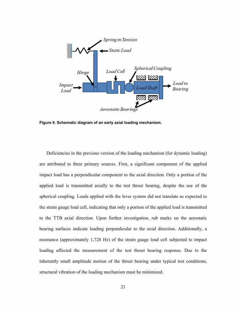
exerted along the axial direction. Figure 9 shows a schematic of an early version of the
loading mechanism which utilizes a lever to apply a static load from a spring in tension
and dynamic load through an impact load to the base. A load cell located on the tip of an
impact hammer records the impulse load while a strain gauge load cell mounted in series
with the loader and the load shaft measures the static load applied by the spring/lever
system. A spherical coupling between the load cell and load shaft is used to reduce the
moment applied to the load shaft. This design proved to be effective for application of a
static load but ineffective for dynamic loading (with impact loads).
21
Figure 9. Schematic diagram of an early axial loading mechanism.
Deficiencies in the previous version of the loading mechanism (for dynamic loading)
are attributed to three primary sources. First, a significant component of the applied
impact load has a perpendicular component to the axial direction. Only a portion of the
applied load is transmitted axially to the test thrust bearing, despite the use of the
spherical coupling. Loads applied with the lever system did not translate as expected to
the strain gauge load cell, indicating that only a portion of the applied load is transmitted
to the TTB axial direction. Upon further investigation, rub marks on the aerostatic
bearing surfaces indicate loading perpendicular to the axial direction. Additionally, a
resonance (approximately 1,728 Hz) of the strain gauge load cell subjected to impact
loading affected the measurement of the test thrust bearing response. Due to the
inherently small amplitude motion of the thrust bearing under typical test conditions,
structural vibration of the loading mechanism must be minimized.

22
The strain gauge load cell, used to measure static load, is removed from the system
and suspended with a cable as shown in Figure 10. A simple impact load test identifies
the natural frequency of the strain gauge load cell in the axial direction. An impact
hammer applies a dynamic load to the load cell while an accelerometer records the
vibration, all in the axial direction. Figure 11 shows the structural resonant frequency of
the strain gauge load cell occurs at approximately 1,728 Hz, as measured by a dynamic
signal analyzer. Although the frequency of the structural load cell vibration is higher
than that of the TTB, the vibration amplitude is larger than the axial response of the
bearing which distorts the frequency response of the system. Ultimately, the strain gauge
load cell is removed from the load shaft assembly in favor of a much smaller dynamic
load cell which is better-suited suited for the sampling frequency required for the
dynamic load tests.
Furthermore, the dynamic load measured by the impact gun load cell (mounted to the
tip of the gun) captured only the initial compressive impact load but failed to register the
test thrust bearing forced response, both tensile and compressive. This realization
influenced the move to an integral load cell configuration where the load cell is rigidly
connected as part of the moving load mechanism, as shown in Figure 14. By preloading
the load cell during the assembly process, both tensile and compressive load
measurements are possible.

23
Figure 10. Impact load test to determine resonant frequency of a strain gauge load cell.
Figure 11. Dynamic signal analyzer output of strain gauge load cell impact test showing a resonant frequency at 1728 Hz with good coherence between the delivered impact load (input) and the measured acceleration (output).

24
Consequently, the loading mechanism is redesigned to better direct impact loads
axially, to reduce resonant load cell interference, and to capture the test thrust bearing
forced response. Figure 12 shows a diagram of the resulting taut cable system, and
Figure 13 displays a photograph of the mechanism. A taut steel cable is routed through a
hollow head impact tip to apply a static load to the system. One end of the impact tip is
fastened rigidly to a load cell which is, in turn, threaded directly into the load shaft,
while a flat surface on the opposite end receives impulse loads from an impact gun, as
shown in Figure 14. The static load magnitude is controlled by adjusting the cable
tension, while the magnitude of the impact load is configured through the impact
hammer settings. The direction of the resultant load is manipulated by positioning the
fixed ends of the cable using a pair of adjustable brackets. The result is a superimposed
static and dynamic load oriented along just the axial direction, as desired. The dynamic
load is measured with a load cell fastened between the impact tip and the load shaft. This
load cell has an initial pre-load during installation so as to measure both compressive
and tensile loads. The static load is derived using the system geometry, shown in Figure
12, and the cable tension, measured using a strain gauge load cell. The braided steel
cable is 1.5 mm in diameter, and its stiffness is 93.15 ± 0.29 kN/m (see Appendix D for
its estimation). By relocating the strain gauge load cell away from the axial load path,
the resonant structural vibration of the instrument is no longer excited by the impact and,
therefore, no longer interferes with the test thrust bearing response measurement.
Figure 15 shows measured accelerations from an axially mounted sensor on the TTB
housing with (a) the previous configuration and (b) the new loading mechanism.

25
Increasing the structural stiffness of the loading mechanism reveals an overdamped
system, as shown in Figure 15(b). Note that a third load cell, mounted at the tip of the
impact hammer, triggers the data acquisition system.
Figure 12. Schematic of redesigned, cable-loaded loading system and the geometry of the taut cable used to derive the equivalent static load along the axial direction, Fr.

26
Figure 13. Photograph of taut cable load mechanism.
27
Figure 14. Photograph of the updated impact tip/load cell assembly. The dynamic load cell utilizes a threaded connection to both the impact tip and the load shaft. Preload is set by tensioning these threaded connections, enabling the dynamic load cell to measure both compressive and tensile forces.
(a) Prior configuration (b) Current configuration with taut
cable
Figure 15. Axial acceleration measurements on TTB housing due to an impact load (a) with early configuration of load mechanism, and (b) with new configuration with taut cable.
28
SYSTEM MODEL FOR PARAMETER IDENTIFICATION
Thrust bearing force coefficients (stiffness KTTB, damping CTTB, and added mass
MTTB) enable the prediction and control of axial rotor motions under dynamic loading.
Obtaining reliable estimates of the bearing operating performance in actual test
conditions is (although challenging) necessary to validate predictive models [18].
Figure 16 shows a schematic view of the test thrust bearing and load shaft assembly
modeled as a one degree of freedom (1-DOF) system1. Let TTBz and Rz be the absolute
axial displacements of the TB and rotor, respectively, and TTB Rz z z is the relative
displacement between both components. Additionally, a taut steel cable with stiffness
KCable applies the static force to the load shaft. A simple load vs. displacement
experiment determines KCable as detailed in Appendix D. In Figure 16, a linear viscous
damper (CTTB), stiffness (KTTB), and mass (MTTB) coefficients denote the reaction of the
thrust fluid film bearing.
1 Model assumes no dynamic tilts or rotation, aligned rotor thrust collar and TTB face.

29
Figure 16. Schematic view of 1-DOF model of test TB for parameter identification.
The instrumentation used during the dynamic load tests includes six eddy current
sensors (three on each thrust bearing), one piezoelectric accelerometer affixed to the test
thrust bearing cartridge along the axial direction, and one load cell mounted on one end
of the static loader. Three eddy current sensors define a plane and enable determination
of the operating clearance at the center (C0) of both the test TB and slave TB, as well as
the tilt angles, if any.
At a static equilibrium, the applied load (from the taut cable) is balanced by the
test TB force, , generated by an equilibrium clearance C0= zo. Due to an impact
load, , the test element (thrust bearing) in Figure 16 undergoes small amplitude
30
motions about its static equilibrium position. The test and slave thrust bearings react to
the dynamic force. Eddy current sensors record the ensuing motion while an
accelerometer affixed to the load shaft assembly measures its acceleration ( TTBz ).
Assuming no axial drag from the aerostatic bearings, the equation of motion (EOM)
for the system undergoing axial motions is:
M TTB TTBd a et C blFz F F (1)
where M = 2.538 kg is the mass of the load shaft, TB and load cell, is an applied
impact load, CableF is the axial force applied by the taut cable on the load shaft
(2Tcos60°), and TTBF is the TTB reaction force equal to 0 dTTB TTB TTB tF F F . ZTTB
represents TTB axial displacement and ZR represents the axial displacement of the rotor
as shown in Figure 16.
Assuming a massless and undamped cable, the force exerted by the cable is:
(2)
Where Kcable is the axial stiffness of the cable loading system. Appendix D describes the
experimental apparatus to determine this stiffness.
At equilibrium,
0TTBF 0T (3)
Represent the dynamic component of the TTB force as
(4)
where , , and are the bearing axial force coefficients (stiffness, damping
and added mass, respectively). Hence, Eq. (1) becomes

31
(5)
The discrete Fourier transform (DFT) algorithm transforms force, displacement and
acceleration data from the time domain into the frequency domain [11]. Let
( ) ( )
, , , zt tt t TTBTTB TTBzz DFT z F DFT F A DFT zDFT (6)
where ω denotes frequency. Recall that
ti z DFT z ; 2
tz DFT z (7)
where √ 1 is the imaginary unit. Hence, in the frequency domain Eq. (5) becomes
2
2Cabled
TTB TTB TTB
F M AH K M i C
z
K
(8)
Where H is the complex dynamic stiffness for the test element. With H obtained, the
estimation of the TB axial force coefficients follows from curve fitting of the real and
imaginary parts of the complex dynamic stiffness, i.e.
2 , TTBTTB
Re H K M Im H C (9)

32
DATA ACQUISITION AND PROCESSING
Data Acquisition
Two visual interface (VI) programs are written for impact load testing. The first VI
uses to control the automatic impact hammer, through an analog voltage output module.
The system is capable of delivering a specified number of impulse loads at a defined
time interval. Typically, impacts are delivered on 5 second intervals to allow ample time
for the system to settle back into an equilibrium axial position after excitation.
Figure 17 shows the second VI used to record impact test data. A load cell mounted
on the tip of the automatic impact hammer is used as a trigger to begin data acquisition.
Triggering parameters are configured directly from the VI. Once the trigger signal
surpasses the specified level, the program records data, including a defined number of
pre-trigger samples (a standard 10 pre-trigger samples are taken for all test conducted
herein). The number of samples taken per test and the sampling frequency are also
configured on the VI. For the subsequent Fast Fourier Transform (FFT) analysis, the
number of data points must be a power of two; however, an additional two samples are
needed to differentiate the recorded displacement signal for comparison with the
recorded acceleration signal which drives the selection of 214+2 = 16,386 samples/test.
With this sampling rate and the number of instruments used, the maximum sampling rate
for the data acquisition chassis is used, 31,250 Hz, yielding 0.52 seconds of recorded
data for each test. The graph towards the top of the VI shown in Figure 17 reveals raw
data from each test and is used for quick, real-time data quality assurance.
33
Figure 17. Visual Interface (VI) front panel recording dynamic impact test data.
The coherence between the load shaft acceleration and the impact load is monitored
in real-time. A sound frequency identification range is determined for the region of
coherence, S~1. Coherence results are remarkably consistent for frequencies between 0
and 250 Hz for each impact load.
Data Processing
A computational script processes the data recorded by the data acquisition system.
Test parameters including number of impacts, frequency identification range, number of
samples and sampling rate are user-defined. For each test examined herein, 100 impacts
are averaged, each with 16,386 samples recorded at a rate of 31,250 Hz. The frequency
34
identification range is determined in real-time between dynamic load and acceleration
measurements taken with a dynamic signal analyzer.
The clearance (C0) at the center of the TTB is calculated from axial displacements
obtained from three eddy current proximity sensors installed on the TTB housing.
Appendix B details the derivation of the TTB center clearance based on the three eddy
current probe measurements and their fixed angular positions on the TTB face.
The frequency domain data provides the complex dynamic stiffness, H(ω). Real and
imaginary parts of H(ω) are separated and then averaged for each test condition. Figure
18
shows an example of a linear curve fit for the average real and imaginary parts of H(ω)
from 100 impacts. The axial force coefficients are determined using Eqn. (9).

35
Figure 18. Sample linear curve fit of the (a) real and (b) imaginary portions of the TTB complex stiffness (H) vs frequency. W/A is the specific load defined as the axial load per unit area. Note that A = 32.6 cm2.

36
THRUST BEARING PERFORMANCE
A series of tests are used to quantify the static and dynamic load performance of the
test TTB for rotor speeds up to 6 krpm (ΩRout=23.9 m/s). The next sections will outline
both static and dynamic load test matrices as well as the results. Static load tests examine
the effect of TTB supply pressure, applied axial load and shaft speed on the TTB axial
clearance. Dynamic load tests examine the effect of these variables on the TTB bearing
force coefficients, namely stiffness, damping and added mass. For all test conditions,
water at a pressure of 3.45 bar(g) lubricates the radial bearings.

37
STATIC LOAD PERFORMANCE
Static load measurements are followed immediately by dynamic load tests. This is
done to maximize repeatability of impacts during dynamic testing. This method
necessitates the test rig instrumentation to be configured for dynamic load testing.
Therefore, static load test results are limited to data acquired by the high speed data
acquisition system used for dynamic testing, namely applied axial load and thrust
bearing axial clearance.
At a null rotor speed, water supplies the axial test and slave thrust bearings with an
increasing inlet pressure. Static load is then applied to the test thrust bearing using the
cable tension loading system causing the bearing to load the rotor thrust collar. The
specific static load, i.e., load per unit area (W/A) is used as a load metric. Note A = 32.6
cm2 = ¼ π (Dout2-Din
2). The slave thrust bearing reacts to the applied load, thereby
controlling rotor position. Finally, the electric motor gradually spins the rotor-coupling
system up to test speed. Test speeds up to 6 krpm are performed, corresponding to a
maximum surface speed of 24 m/s on the edge of the rotor thrust collar (Rout=7.62 cm).
The TTB supply pressure is measured using a pressure transducer positioned just
upstream of the thrust bearing. With the supply pressure held constant, the static load
system applies a decreasing load to the test thrust bearing. A decreasing load is applied
to ensure that the lowest clearance (highest load) condition enables the rotor to spin
freely at the onset of testing to avoid risk of contact between the rotor and TTB for
subsequent load conditions. If the rotor does not spin freely the load shaft and TTB
assembly must be aligned to the rotor thrust collar. After the conclusion of a static load

38
condition, the motor stops, and the process repeats for the remaining supply pressure
conditions.
Static Load Tests at Various Supply Pressures and Rotor Speeds
Table 1 outlines the static load test matrix designed to quantify the effects of distinct
supply pressures and rotor speeds on the TTB static load performance at various applied
load conditions. Figure 19 through Figure 22 present axial clearance vs. axial specific
load (W/A) for rotor speeds ranging from 3krpm to 6krpm, respectively. The curves
represent operation at TTB supply pressure of 2.76 bar(g), 3.45 bar(g), 4.14 bar(g) and
4.83 bar(g). Horizontal error bars represent uncertainty of the applied axial load while
the vertical error bars represent the uncertainty of the calculated axial clearance at the
center of the TTB. The large uncertainty2 shown in Figures 21 through 28 are due to the
allowable runout of each thrust collar (±10 μm). Appendix C presents a description of
the uncertainty analysis is presented.
Table 1. Test Matrix for static load tests at null to moderate shaft speed.
Shaft Speed (krpm)
TTB Supply Pressure (bar(g))
Specific Load (W/A) (bar)
0, 3, 4, 5, 6
2.75
0.2 – 1.6 3.45 4.14 4.83
Figure 19 includes a solid line representing a sample prediction [2] for the 2.76
bar(g), 3 krpm test condition. Predictions match qualitatively with measurement trends
2 Uncertainty for the static load results indicated with error bars at each data point.

39
although being consistently higher than the corresponding test data, with average percent
differences of 25% to 53% [3]. Prior work [3, 5] presents correlation between static load
measurements and predictions.
At a constant rotational speed, the TTB center clearance (C0) decreases as the
applied specific load increases. The difference in operating axial clearance between
conditions of Ps = 2.76 bar(g) and 4.83 bar(g) is higher at lower clearances (high axial
loads). The load differential decreases as the axial clearance increases (decreasing axial
load). The behavior is consistent for each rotor speed and applied load condition
indicating that TTB supply pressure is the primary factor affecting its static load
performance. Note the axial clearance increases with an increase in TTB supply
pressure.
Figure 19. Axial clearance (C0) versus specific load (W/A) for operation at four TTB supply pressures (Ps) and rotor speed at 3 krpm. Horizontal error bars represent the uncertainty in the axial load at a 95% confidence interval. Vertical error bars indicate the uncertainty in the axial clearance due to the machined runout of the rotor.
40
Figure 20. . Axial clearance (C0) versus specific load (W/A) for operation at four TTB supply pressures (Ps) and rotor speed at 4 krpm. Horizontal error bars represent the uncertainty in the axial load at a 95% confidence interval. Vertical error bars indicate the uncertainty in the axial clearance due to the machined runout of the rotor.
Figure 21. . Axial clearance (C0) versus specific load (W/A) for operation at four TTB supply pressures (Ps) and rotor speed at 5 krpm. Horizontal error bars represent the uncertainty in the axial load at a 95% confidence interval. Vertical error bars indicate the uncertainty in the axial clearance due to the machined runout of the rotor.

41
Figure 22. . Axial clearance (C0) versus specific load (W/A) for operation at four TTB supply pressures (Ps) and rotor speed at 6 krpm. Horizontal error bars represent the uncertainty in the axial load at a 95% confidence interval. Vertical error bars indicate the uncertainty in the axial clearance due to the machined runout of the rotor.
Static Load Tests at Various Rotor Speeds
To quantify the effect of shaft speed on TTB static load performance, Figure 23
through Figure 26 show the axial clearance (C0) vs. axial specific load for TTB supply
pressures of 2.76 bar(g), 3.45 bar(g), 4.14 bar(g), and 4.83 bar(g), respectively. Rotor
speeds of 0 krpm through 6 krpm are labeled on each graph.
At a constant TTB supply pressure (PS), the axial clearance decreases marginally
while the speed reduces from 6krpm to 3krpm. The axial clearance differential is larger
at a lower axial clearance (higher load), indicating that the hydrodynamic component of
the bearing reaction force is larger at small axial clearance. The null rotor speed
condition represents pure hydrostatic operation.

42
Figure 23. Axial clearance (C0) versus specific load (W/A) for operation at various rotor speeds for operation with supply pressure Ps = 2.76 bar(g). Horizontal error bars represent the uncertainty in the axial load at a 95% confidence interval. Vertical error bars indicate the uncertainty in the axial clearance due to the machined runout of the rotor.
Figure 24. Axial clearance (C0) versus specific load (W/A) for operation at various rotor speeds for operation with supply pressure PS = 3.45 bar(g). Horizontal error bars represent the uncertainty in the axial load at a 95% confidence interval. Vertical error bars indicate the uncertainty in the axial clearance due to the machined runout of the rotor.
43
Figure 25. Axial clearance (C0) versus specific load (W/A) for operation at various rotor speeds for operation with supply pressure PS = 4.14 bar(g). Horizontal error bars represent the uncertainty in the axial load at a 95% confidence interval. Vertical error bars indicate the uncertainty in the axial clearance due to the machined runout of the rotor.
Figure 26. Axial clearance (C0) versus specific load (W/A) for operation at various rotor speeds for operation with supply pressure PS = 4.83 bar(g). Horizontal error bars represent the uncertainty in the axial load at a 95% confidence interval. Vertical error bars indicate the uncertainty in the axial clearance due to the machined runout of the rotor.

44
Static load results presented by Rohmer [15] match well with the current results for
operation at null and 3 krpm rotor speed, and up to 4.14 bar(g) TTB supply pressure.
Namely, the TTB axial clearance (C0) increases as water supply pressure (Ps) increases
under a constant applied load. The magnitude of said clearance is consistent with
Rohmer’s results [15], further verifying the performance of the test rig after extensive
modification to the fluid supply system and axial loading mechanism.
45
DYNAMIC LOAD PERFORMANCE
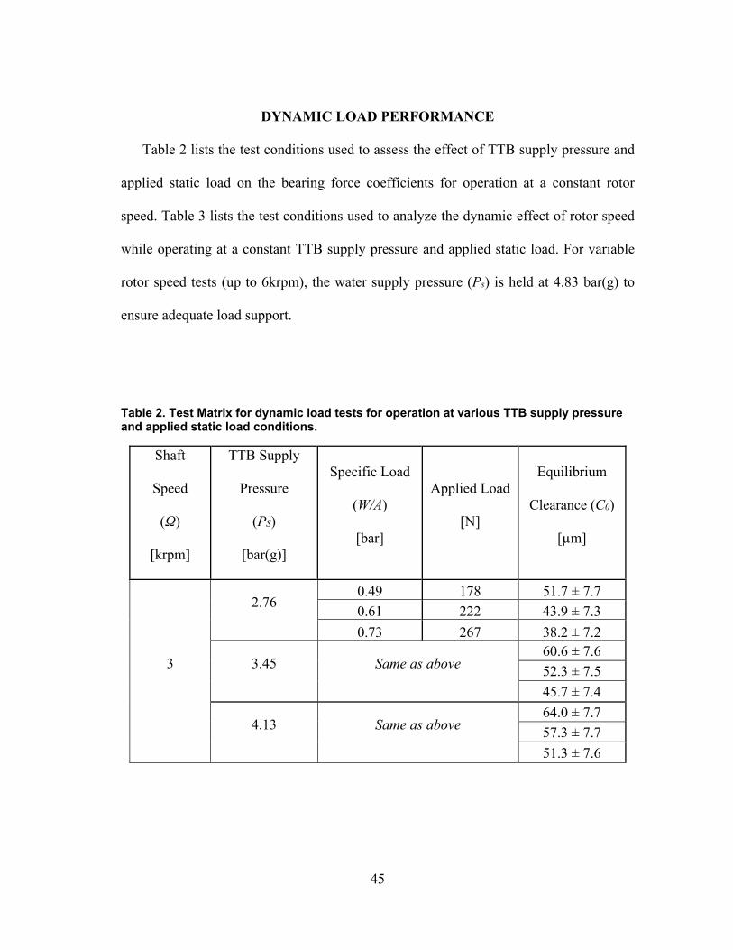
Table 2 lists the test conditions used to assess the effect of TTB supply pressure and
applied static load on the bearing force coefficients for operation at a constant rotor
speed. Table 3 lists the test conditions used to analyze the dynamic effect of rotor speed
while operating at a constant TTB supply pressure and applied static load. For variable
rotor speed tests (up to 6krpm), the water supply pressure (Ps) is held at 4.83 bar(g) to
ensure adequate load support.
Table 2. Test Matrix for dynamic load tests for operation at various TTB supply pressure and applied static load conditions.
Shaft
Speed
(Ω)
[krpm]
TTB Supply
Pressure
(PS)
[bar(g)]
Specific Load
(W/A)
[bar]
Applied Load
[N]
Equilibrium
Clearance (C0)
[µm]
3
2.76 0.49 178 51.7 ± 7.7
0.61 222 43.9 ± 7.3
0.73 267 38.2 ± 7.2
3.45 Same as above 60.6 ± 7.6
52.3 ± 7.5
45.7 ± 7.4
4.13 Same as above 64.0 ± 7.7
57.3 ± 7.7
51.3 ± 7.6

46
Table 3. Test Matrix for dynamic load tests for operation at null to moderate shaft speeds.
Shaft Speed (krpm)
TTB Supply
Pressure (bar)
Specific Load (bar)
Applied Load (N)
Equilibrium Clearance (C0)
(µm)
0
4.83
0.49 178 85.3 ± 1.1
0.61 222 72.7 ± 1.3
0.73 267 60.1 ± 1.5
3 Same as above
68.1 ± 7.6
63.8 ± 7.7
57.5 ± 7.7
4 Same as above
69.3 ± 7.6
65.9 ± 7.7
62.5 ± 7.7
5 Same as above
77.9 ±7.6
72.4 ± 7.6
66.8 ± 7.7
6 Same as above
77.2 ± 7.6
73.1 ± 7.6
68.9 ± 7.7
Dynamic Load Tests at Various Supply Pressures and a Fixed Rotor Speed
Prior to initiating motor speed, 3.45 bar(g) pressurized water flows into the radial
bearings allowing the rotor to spin freely by hand. Water then supplies the axial test and
slave thrust bearings with a constant pressure, Ps, as prescribed by Table 2. The cable
tension loading system shown in Figure 12 applies the prescribed static load. The slave
thrust bearing reacts to the applied load. The electric motor gradually spins the rotor-
coupling system up to a speed of 3krpm. Upon meeting the test condition, a series of
47
impact loads excite the load shaft and thrust bearing in the axial direction. Impact data
sets are individually converted into the frequency domain and then averaged. The
process repeats for supply pressures of 2.76, 3.45 and 4.13 bar(g).
Figure 27 shows the identified thrust bearing stiffness ( ) vs. water supply pressure
(Ps) and operation at 3 krpm shaft speed. With an increase in supply pressure, the axial
stiffness increases. This behavior correlates well with the predicted stiffness [2] although
the rate of increase is higher than that of the experimental magnitude. A change in
applied axial load has minimal influence on , indicating that Ps is the primary driver of
stiffness .
Error bars shown in the bearing coefficient results below indicate the measurement
uncertainty associated with the dynamic load testing method. The large uncertainty is
due in part to the allowable run out of the thrust collar (±10µm) and the repeatability
uncertainty associated with the load impact tests as detailed in Appendix C.
Repeatability uncertainty is low compared to the uncertainty of clearance measurements.

48
Figure 27. Experimentally measured and predicted axial stiffness coefficient (Kz) for TTB operating with water supplied at 2.75, 3.45 and 4.14 bar(g) and shaft speed of 3 krpm. Applied specific axial load, W/A = 0.49 bar, 0.61 bar, and 0.73 bar.
Figure 28 shows the axial damping ( ) vs. water supply pressure (Ps) and operation
at 3 krpm shaft speed. The graph shows data for three applied specific load conditions,
W/A = 0.49, 0.61, and 0.73 bar. The predicted damping increases with an increase in
supply pressure. The qualitative increase in measured damping agree with predictions
although the magnitude of the measured damping values exceeds predictions for all but
the Ps = 3.45 bar(g), W/A = 0.61 bar specific load test condition. A change in applied
axial load has minimal influence on , although for Ps = 2.76 bar(g) identified
coefficients decreases with increasing load. Similar to stiffness , TB supply pressure
Ps influences damping more than applied load.

49
Figure 28. Measured and predicted damping coefficient (Cz) for TTB operating with water supplied at 2.75, 3.45 and 4.14 bar and shaft speed of 3 krpm. Applied specific axial load, W/A = 0.49 bar, 0.61 bar, and 0.73 bar.
Figure 29 shows the identified added mass (Mz) vs. water supply pressure and
operation at a constant 3krpm shaft speed. The graph presents results for three applied
specific load conditions, W/A = 0.49, 0.61, and 0.73 bar. The added mass coefficient
exceeds the predicted magnitude for all cases (ranging from 8% to 32% difference).
Both predictions and measurements indicate a minimal change in coefficient magnitude
with an increase in water supply pressure. The maximum percent difference between the
maximum and minimum supply pressures, Ps, is only 29% for the W/A = 0.73 bar
applied load case.

50
Figure 29. Measured and predicted added mass coefficient (Mz) for TTB operating with water supplied at 2.75, 3.44 and 4.13 bar and shaft rotational speed of 3 krpm. Applied specific axial loads of 0.49 bar, 0.61 bar, and 0.73 bar.
Dynamic Load Tests at Various Rotor Speeds and a Fixed Supply Pressure
3.45 bar(g) pressurized water flows into the radial bearings allowing the rotor to spin
freely by hand before starting the electric motor. Water then supplies the axial test and
slave thrust bearings with a constant pressure, Ps = 4.83 bar(g). The cable tension
loading system shown in Figure 12 applies progressively decreasing TTB static load.
The slave thrust bearing reacts to the applied load. The electric motor gradually spins the
rotor-coupling system up to test speed. Upon meeting the prescribed dynamic load test
condition, a series of impact loads excite the load shaft and thrust bearing in the axial
direction. Impact data sets are individually converted into the frequency domain and then
51
averaged. The process repeats for shaft speeds increasing from 3 krpm to 6 krpm as
indicated in Table 3.
Figure 30 shows measured and predicted stiffness (Kz) vs. rotor speed for static
loads, W/A = 0.49, 0.61 and 0.73 bar, with a constant 4.83 bar TTB supply pressure. As
expected, as the static load increases, the bearing stiffness Kz also increases. As rotor
speed increases, however, Kz does not change appreciably. Both measurements and
predictions capture this behavior, this indicating the TTB performs primarily as a
hydrostatic bearing.
Figure 30. Measured and predicted stiffness (Kz) for the TTB operating with water supplied 4.83 bar and shaft speed of 3 krpm, 4krpm, 5krpm and 6krpm. Specific axial load W/A = 0.49 bar, 0.61 bar, and 0.73 bar is applied to the TTB.

52
Figure 31 shows measured and predicted damping (Cz) vs. increasing rotor speed for
the test thrust bearing subjected to three applied static loads, W/A = 0.49, 0.61 and 0.73
bar, with 4.83 bar TTB supply. Both predictions and measured results indicate a
minimal change in damping (Cz) with an increase in rotor speed, while Cz increases as
the static load increases. Although the test damping magnitude exceeds the predicted
values for W/A = 0.73 bar, the magnitudes of predictions and measurements agree well
overall.
Figure 31. Measured and predicted damping (Cz) for the TTB operating with water supplied at 4.83 bar psi(g) and shaft speed of 3 krpm, 4krpm, 5krpm and 6krpm. Specific axial load W/A = 0.49 bar, 0.61 bar, and 0.73 bar is applied to the TTB.
Figure 32 shows the experimental added mass (Mz) vs. rotor speed for the TTB under
three applied static loads, W/A = 0.49, 0.61 and 0.73 bar, with 4.83 bar TTB supply

53
pressure. Predictions show no significant change in added mass with a change in shaft
speed or applied load. The test results qualitatively agree with the prediction that Mz is
minimally influenced by rotor speed. However, the magnitude of the test results exceed
the predictions and indicate an increase in Mz with an increase in applied static load.
Figure 32. Measured and predicted added mass (Mz) for the TTB operating with water supplied at 4.83 bar psi(g) and shaft speed of 3 krpm, 4krpm, 5krpm and 6krpm. Specific axial load W/A = 0.49 bar, 0.61 bar, and 0.73 bar is applied to the TTB.

54
CONCLUSION
After a successful static load testing campaign in 2015 [16], the thrust bearing test
rig was modified to conduct dynamic tests to determine bearing force coefficients
(stiffness, damping and added mass). Reliable lubrication flow is provided by a new,
continuous water supply system designed to run continuously for long periods of time as
required for dynamic testing and with little waste. Additionally, an innovative loading
system enables simultaneous application of static and dynamic loads via a taut cable and
an automated impact hammer. Ultimately, these modifications allow for more controlled
and repeatable test conditions which benefit acquisition of both static load and dynamic
load test data. The experimental results validate model predictions and augment the
bearing design process for future projects.
Prior to testing for bearing force coefficients, static load measurements are taken.
These results further validate effectiveness of the test rig in determining static force vs.
displacement performance and confirm that the rig is functioning properly after
modification to accommodate the dynamic loading mechanism and new water supply
system. The measured static load behavior match well with predictive software as well
as prior experimental results. At a constant axial load, the axial clearance (C0) increases
as the TTB lubrication pressure (Ps) increases. With a constant supply pressure (Ps),
however, the test TB axial clearance (C0) decreases as the applied axial load (W/A)
increases. Large uncertainties, inherent with the test rig, continue to plague axial
displacement measurements.

55
For operation at a moderate shaft speed (up to 6krpm), dynamic behavior of a water
lubricated thrust bearing is measured through impact load testing and quantified with
force coefficients derived from the system complex dynamic stiffness function.
Measurements indicate that the test thrust bearing shows no appreciable change in
dynamic force coefficients (axial stiffness, damping and inertia) with a change in rotor
speed. This behavior proves the bearing behaves in a mainly hydrostatic mode as it lacks
hydrodynamic features on the bearing surface such as tapered sections or tilting pads. In
short, the bearing behaves as a purely hydrostatic bearing for the range of rotor speeds
examined herein. With an increase in applied static load, however, the test bearing
stiffness and damping increase while added mass does not show appreciable change. The
measured bearing dynamic behavior with increasing static load corresponds well with
predicted values. Finally, with a constant applied load and low rotor speed (3krpm), an
increase in TB supply pressure increases the stiffness and damping coefficients but does
not bearing inertia.
Uncertainties associated with the axial clearance measurements are large for static
and dynamic load tests. This uncertainty is largely due to the runout tolerance of the
rotor thrust collar. To mitigate this uncertainty in future tests, a new rotor could be
machined with tighter tolerances for this critical dimension.

56
REFERENCES
[1] Rohmer, M. and San Andrés, L., 2014, “Revamping a Thrust Bearing Test Rig,”
Annual Progress Report to the Turbomachinery Research Consortium, TRC-B&C-
03-2014, Turbomachinery Laboratory, Texas A&M University, May.
[2] San Andrés, L., 2002, “Effects of Misalignment on Turbulent Flow Hybrid Thrust
Bearings,” ASME J. of Trib., 124(1), pp. 212-219.
[3] Rohmer, M., San Andrés, L., and Wilkinson, S. 2018, “Static Load Performance of a
Water-Lubricated Hydrostatic Bearing,” J. Eng. Gas Turbines Power, 140(6), pp.
062401-062401-10.
[4] San Andrés, L., Childs, D., and Phillips, S., 2016, “A Water Lubricated Hybrid
Thrust Bearing: Measurements and Predictions of Static Load Performance,” J.
Eng. Gas Turbines Power, 139(2), pp. 022506-022506-10.
[5] San Andrés, L., 2006, “Hybrid Flexure Pivot-Tilting Pad Gas Bearings: Analysis and
Experimental Validation,” ASME J. Tribol., 128, pp. 551-558.
[6] Rowe, W., 1983, Hydrostatic and Hybrid Bearing Design, Textbook, Butterworths,
London, England, pp. 1-20, 46-68.
[7] Nosaka, M. and Kato, T., 2013, Cryogenic Tribology in High-Speed Bearings and
Shaft Seals of Rocket Turbopumps, Textbook, Dr. Jürgen Gegner (Ed.), DOI:
10.5772/55733.
[8] San Andrés, L., 2000, “Bulk-Flow Analysis of Hybrid Thrust Bearings for Process
Fluid Applications,” ASME J. of Trib., 122(1), pp. 170-180.
[9] Safar, Z.S., 1983, “Centrifugal Effects in Misaligned Hydrostatic Thrust Bearings,”

57
ASME J. of Trib., 105, pp. 621-624.
[10] Santiago, O., San Andrés, L., 2007, “Field Methods for Identification of Bearing
Support Parameters- Part I: Identification from Transient Rotor Dynamic Response
due to Impacts,” ASME J. Eng. Gas Turbines Power, 129, pp. 205-212.
[11] San Andrés, L., 2010, “Modern Lubrication Theory, Experimental Identification of
Bearing Force Coefficients,” Notes 14, Texas A&M University Digital Libraries,
http://oaktrust.library.tamu.edu/handle/1969.1/93254 [5 April 2016].
[12] Forsberg, M., (2008), “Comparison Between Predictions and Experimental
Measurements for an Eight Pocket Annular Hydrostatic Thrust Bearing,” Final
Report, Texas A&M University, May-College Station, TX
[13] Ramirez, F., 2008, “Comparison between Predictions and Measurements of
Performance Characteristics for an Eight Pocket Hybrid (Combination
Hydrostatic/Hydrodynamic) Thrust Bearing,” M.S. Thesis, Mechanical Engineering,
Texas A&M University, College Station, TX.
[14] Esser, P., 2010, “Measurements versus Predictions for a Hybrid (Hydrostatic plus
Hydrodynamic) Thrust Bearing for a Range of Orifice Diameters,” M.S. Thesis,
Mechanical Engineering, Texas A&M University, College Station, TX.
[15] Rohmer, M., 2015, “A Test Rig to Measure the Static Load Performance of a Water
Lubricated Thrust Bearing,” M.S. Thesis, Mechanical Engineering, Texas A&M
University, College Station, TX.

58
[16] Rohmer, M., Wilkinson, S. and San Andrés, L., 2015, “Revamping and Preliminary
Operation of a Thrust Bearing Test Rig,” Annual Progress Report to the
Turbomachinery Research Consortium, TRC-B&C-03-2015, Turbomachinery
Laboratory, Texas A&M University, College Station, TX.
[17] Rohmer, M., Wilkinson, S., Jani, H. and San Andrés, L., 2016, “Measurement of
Static Load Performance in a Water Lubricated Hybrid Thrust Bearing,” Annual
Progress Report to the Turbomachinery Research Consortium, TRC-B&C-03-16,
Texas A&M University, College Station, TX, May.
[18] Tiwari, R., Lees, A.W., Friswell, M.I. 2004, “Identification of Dynamic Bearing
Parameters: A Review,” Shock Vib. Dig., 36, pp. 99-124.
[19] Coleman, H. and Steel, W., 1989, “Experimentation and Uncertainty Analysis for
Engineers,” John Wiley and Sons, Inc., pp. 1-71.

59
APPENDIX A
INSTRUMENTATION
Table 4. Instrumentation utilized for TTB dynamic load testing
Name Model/Serial Number Sensitivity (Manufacturer)
Linearity (Manufacturer)
TT1 Proximity Sensor
SKF CMSS65-002-00-12-10 61112 11
7.87 mV/um ±5%
TT2 Proximity Sensor
SKF CMSS65-002-00-12-10 61112 12
7.87 mV/um ±5%
TT3 Proximity Sensor
SKF CMSS65-002-00-12-10 61112 01
7.87 mV/um ±5%
Accelerometer PCB 353 B15/89602 9.81 mV/g ±10% Strain Gauge Load Cell
Omega Engineering LC101-500/ 340069
16.71 mV/lbf ±0.03%
Dynamic Load Cell PCB 208 M51/ 7192 14 mV/lbf ±15%

60
APPENDIX B
ROTOR THRUST COLLAR PLANE EQUATION DERIVATION Thrust Collar Plane Equation
Forsberg [12] prepared the following original analysis. Eddy current sensors face a
thrust collar and measure the axial gap between the thrust collar and TB surface at three
circumferential locations, as shown in Figure 33. Using the gap clearances and the
geometry to determine the clearance between the thrust collar and the TB surface at the
center of the TB and the tilt of the thrust collar relative to the TB is critical in order to
estimate the TB performance.
Figure 33: Reference diagram of a thrust bearing for geometric calculation of clearance as a function of displacements recorded at T1, T2, and T3.
Table 5 describes the horizontal and vertical positions of each eddy current
sensor relative to the center of the TB.

61
Table 5. Horizontal and vertical positions of each eddy current sensor relative to the center of the thrust bearing.
X yProbe T1 Probe T2
x1 = -33.02 mm x2 = -37.34 mm
y1 = 27.69 mm y2 = -21.59 mm
Probe T3 x3 = 37.34 mm y3 = -21.59 mm
Assuming the TB and the thrust collar act as rigid planes, the gap between the
thrust collar and the TB surface at each eddy current sensor can be used with the
position of each eddy current sensor to determine the equation of the plane of the rotor
thrust collar relative to the TB. To derive the rotor thrust collar plane equation, first
establish a vector to define the distance from the TB center to each sensor and the
angle between each vector and the x-axis as,
, tan /
(C1)
respectively.
The axial gap at the center of the TB (C0) as well as the tilt of the rotor thrust collar
about the x-axis (δx) and y-axis (δy) relative to the TB define the clearance at any point
on the thrust collar surface (Ci),
cos sin
(C2)
which can be simplified to the following form,
Y
(C3)
The transformation matrix,
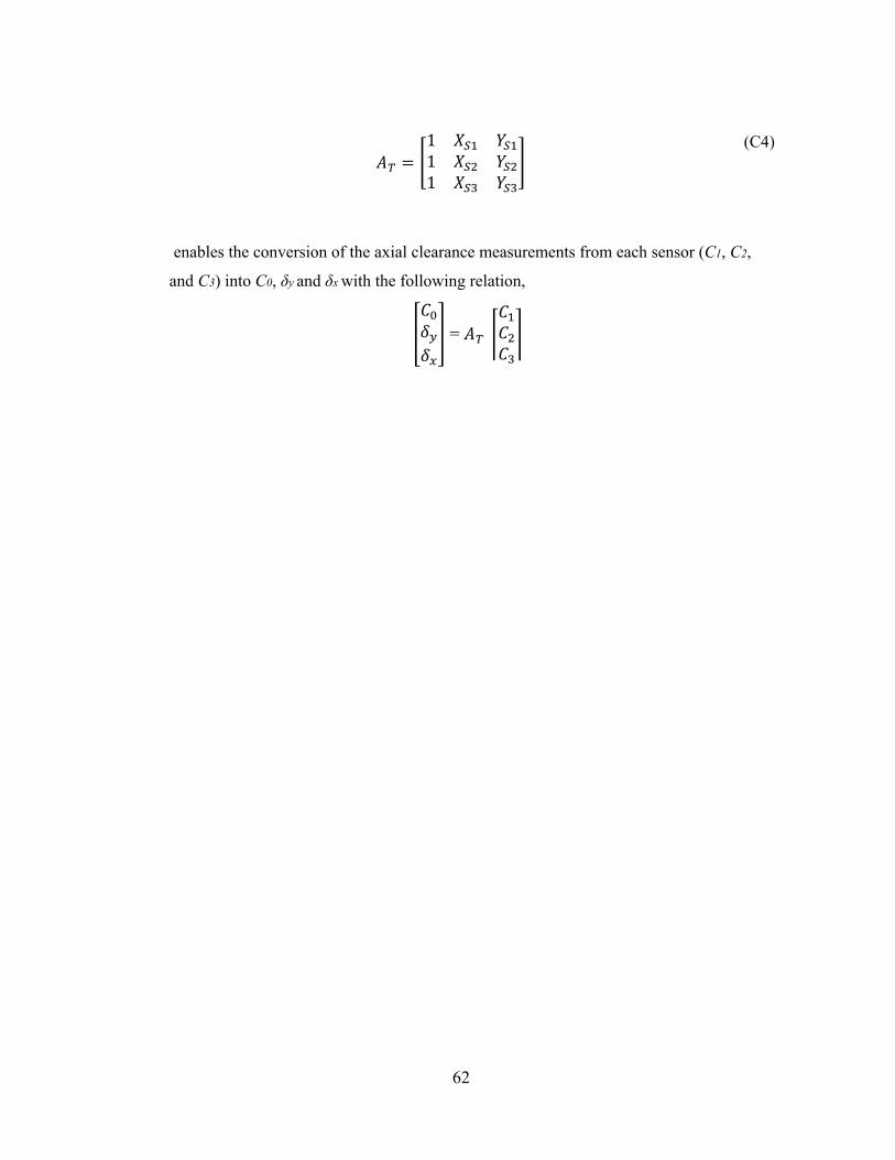
62
111
(C4)
enables the conversion of the axial clearance measurements from each sensor (C1, C2,
and C3) into C0, δy and δx with the following relation,
=
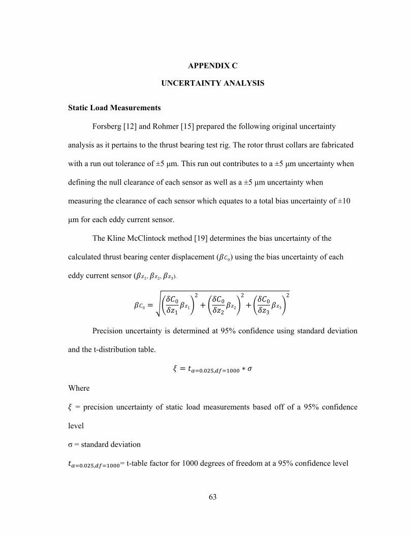
63
APPENDIX C
UNCERTAINTY ANALYSIS
Static Load Measurements
Forsberg [12] and Rohmer [15] prepared the following original uncertainty
analysis as it pertains to the thrust bearing test rig. The rotor thrust collars are fabricated
with a run out tolerance of ±5 μm. This run out contributes to a ±5 μm uncertainty when
defining the null clearance of each sensor as well as a ±5 μm uncertainty when
measuring the clearance of each sensor which equates to a total bias uncertainty of ±10
μm for each eddy current sensor.
The Kline McClintock method [19] determines the bias uncertainty of the
calculated thrust bearing center displacement ( 0) using the bias uncertainty of each
eddy current sensor ( 1, 2, 3).
00
11
20
22
20
33
2
Precision uncertainty is determined at 95% confidence using standard deviation
and the t-distribution table.
. , ∗
Where
= precision uncertainty of static load measurements based off of a 95% confidence
level
σ = standard deviation
. , = t-table factor for 1000 degrees of freedom at a 95% confidence level

64
The total uncertainty for static load testing is determined from the precision and bias
uncertainties using the following equation,
Where
εstat = total uncertainty based off of a 95% confidence level for the static load tests
Dynamic Load Measurements
Dynamic load measurements have two primary sources of uncertainty. The first
stems from the aforementioned displacement uncertainty due primarily to the maximum
allowed run out of the thrust collar (±10μm). This static load uncertainty transcends into
the dynamic load measurements as the displacement is used to calculate the complex
stiffness term for each test condition. The second uncertainty source is the repeatability
associated with the dynamic test procedure.
For each test condition, the thrust bearing response from 100 impacts is recorded and
averaged. To determine the repeatability uncertainty, each test is separated into four
series of 25 impacts. Figure 34 shows the average bearing displacement response for
four data series with operation at thrust and journal supply pressures of 3.45 bar (g) and
3krpm shaft speed. For each series, the bearing coefficients are calculated and the
standard deviation is obtained for the added mass, stiffness and damping values.
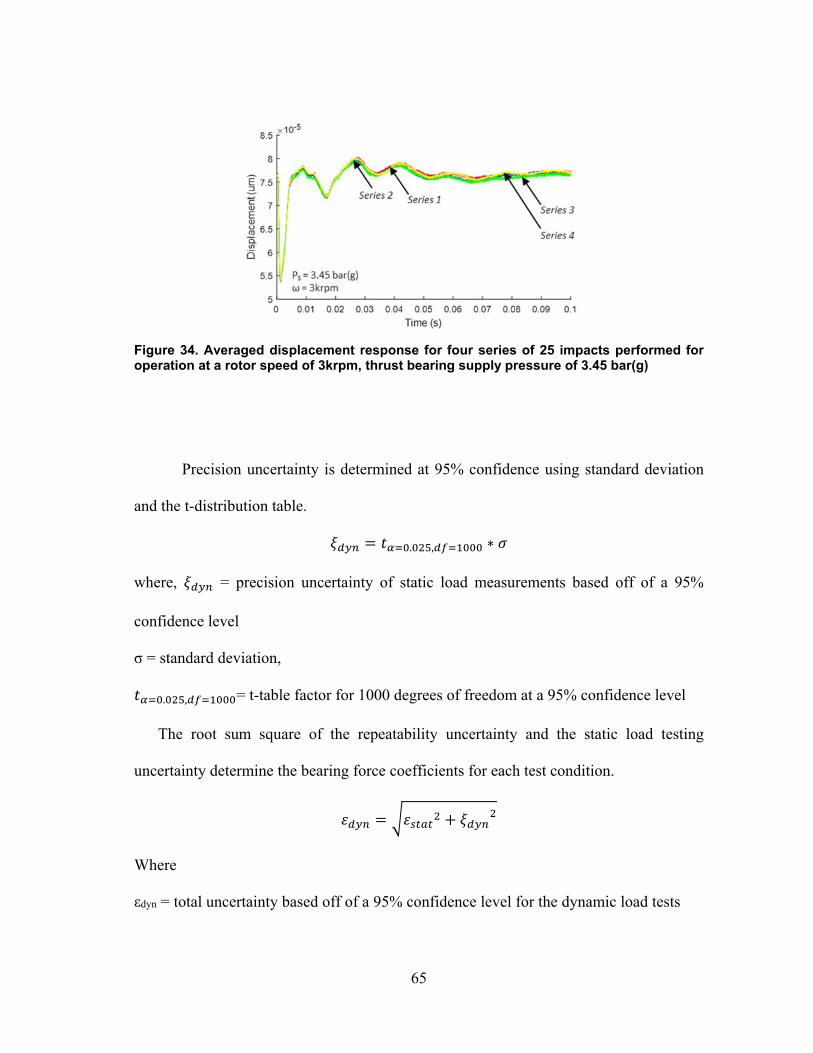
65
Figure 34. Averaged displacement response for four series of 25 impacts performed for operation at a rotor speed of 3krpm, thrust bearing supply pressure of 3.45 bar(g)
Precision uncertainty is determined at 95% confidence using standard deviation
and the t-distribution table.
. , ∗
where, = precision uncertainty of static load measurements based off of a 95%
confidence level
σ = standard deviation,
. , = t-table factor for 1000 degrees of freedom at a 95% confidence level
The root sum square of the repeatability uncertainty and the static load testing
uncertainty determine the bearing force coefficients for each test condition.
Where
εdyn = total uncertainty based off of a 95% confidence level for the dynamic load tests
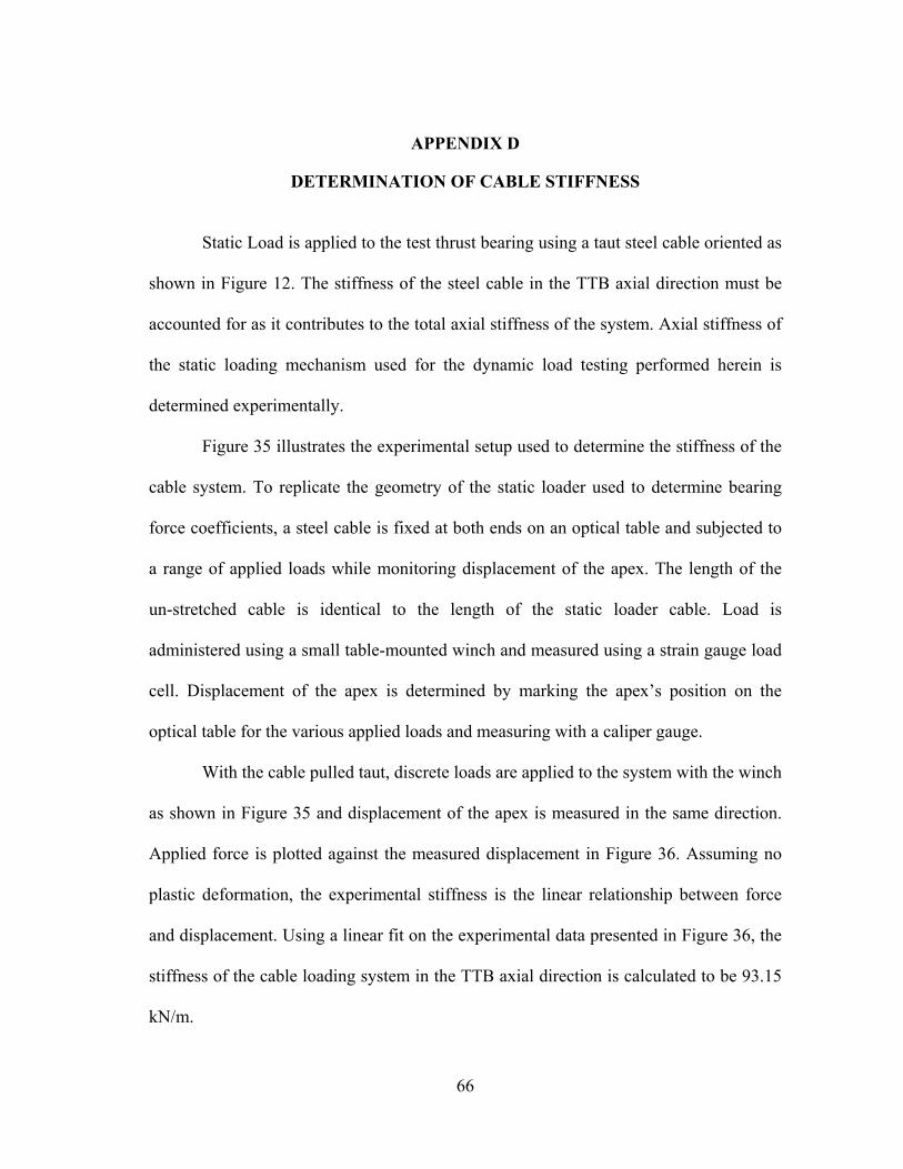
66
APPENDIX D
DETERMINATION OF CABLE STIFFNESS
Static Load is applied to the test thrust bearing using a taut steel cable oriented as
shown in Figure 12. The stiffness of the steel cable in the TTB axial direction must be
accounted for as it contributes to the total axial stiffness of the system. Axial stiffness of
the static loading mechanism used for the dynamic load testing performed herein is
determined experimentally.
Figure 35 illustrates the experimental setup used to determine the stiffness of the
cable system. To replicate the geometry of the static loader used to determine bearing
force coefficients, a steel cable is fixed at both ends on an optical table and subjected to
a range of applied loads while monitoring displacement of the apex. The length of the
un-stretched cable is identical to the length of the static loader cable. Load is
administered using a small table-mounted winch and measured using a strain gauge load
cell. Displacement of the apex is determined by marking the apex’s position on the
optical table for the various applied loads and measuring with a caliper gauge.
With the cable pulled taut, discrete loads are applied to the system with the winch
as shown in Figure 35 and displacement of the apex is measured in the same direction.
Applied force is plotted against the measured displacement in Figure 36. Assuming no
plastic deformation, the experimental stiffness is the linear relationship between force
and displacement. Using a linear fit on the experimental data presented in Figure 36, the
stiffness of the cable loading system in the TTB axial direction is calculated to be 93.15
kN/m.
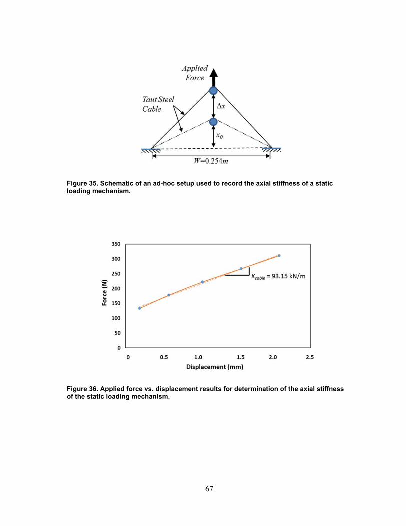
67
Figure 35. Schematic of an ad-hoc setup used to record the axial stiffness of a static loading mechanism.
Figure 36. Applied force vs. displacement results for determination of the axial stiffness of the static loading mechanism.