measurements of and correlations between block size and rock quality designation

Tunnelling and

www.elsevier.com/locate/tust

Tunnelling and Underground Space Technology 20 (2005) 362–377

Underground SpaceTechnologyincorporating Trenchless

Technology Research

Measurements of and correlations between block size androck quality designation (RQD)

Arild Palmstrom *

Norconsult AS, Vestfjordgaten 4, N-1338 Sandvika, Norway

Received 4 November 2004; received in revised form 17 January 2005; accepted 18 January 2005

Available online 3 March 2005

Abstract

Various measurements of the block size or degree of jointing (i.e. density of joints, RQD, block volume, joint spacing) are

described. It is concluded that the RQD measurements are encumbered with several limitations and that this parameter should

be applied with care. These limitations influence the engineering results where RQD is applied in classification systems, numerical

modelling and other engineering assessments.

The three-dimensional block volume (Vb) and the volumetric joint count (Jv) measurements give much better characterizations of

the block size. As the block size forms an important input to most rock engineering calculations and estimates, it is important to

select the most appropriate method to measure this parameter.

Correlations between various measurements of block size have been presented. It turned out difficult to find any reliable corre-

lation between RQD and other block size measurements. An adjusted, better equation between RQD and Jv than the existing is

presented, though still with several limitations.

More efforts should be made to improve the understanding on how to best measure the block size in the various types of expo-

sures and patterns of jointing.

� 2005 Elsevier Ltd. All rights reserved.

Keywords: Block size measurement; RQD; Rock mass jointing; Jointing correlations; Volumetric joint count

1. Introduction

The following three quotations illustrate the back-

ground for this paper:

‘‘Since joints are among the most important causes of

excessive overbreak and of trouble with water, they

always deserve careful consideration.’’ Karl Terzaghi,

1946.

‘‘Provision of reliable input data for engineering design of

structures in rock is one of the most difficult tasks facing

engineering geologists and design engineers. It is extre-

0886-7798/$ - see front matter � 2005 Elsevier Ltd. All rights reserved.

doi:10.1016/j.tust.2005.01.005

* Present address: Ovre Smestad vei 25e, N-0378 Oslo, Norway. Tel.:

+47 6754 4576; fax: +47 6757 1286.

E-mail address: [email protected].

mely important that the quality of the input data matches

the sophistication of the design methods.’’ Z.T. Bieniaw-

ski, 1984.

‘‘I see almost no research effort being devoted to the gen-

eration of the basic input data which we need for our fas-

ter and better models and our improved design

techniques.’’ Evert Hoek, 1994.

Thus, this paper aims at giving practical information

on jointing and input of block size, including:

� different methods to characterize the block size or the

degree of jointing;

� difficulties and errors related to some common meth-

ods to measure rock mass jointing; and

� correlations between various block sizemeasurements.

mailto:[email protected]

Polyhedral blocks

Tabular blocks

Prismatic blocksEquidimensional blocks

Rhombohedral blocks Columnar blocks

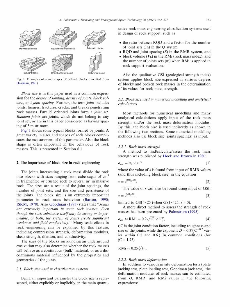
Fig. 1. Examples of some shapes of defined blocks (modified from

Dearman, 1991).

A. Palmstrom / Tunnelling and Underground Space Technology 20 (2005) 362–377 363

Block size is in this paper used as a common expres-

sion for the degree of jointing, density of joints, block vol-

ume, and joint spacing. Further, the term joint includes

joints, fissures, fractures, cracks, and breaks penetrating

rock masses. Parallel oriented joints form a joint set.

Random joints are joints, which do not belong to anyjoint set, or are in this paper considered as having spac-

ing of 5 m or more.

Fig. 1 shows some typical blocks formed by joints. A

great variety in sizes and shapes of rock blocks compli-

cates the measurement of this parameter. Also the block

shape is often important in the behaviour of rock

masses. This is presented in Section 6.1

2. The importance of block size in rock engineering

The joints intersecting a rock mass divide the rock

into blocks with sizes ranging from cube sugar of cm3

in fragmented or crushed rock to several m3 in massive

rock. The sizes are a result of the joint spacings, the

number of joint sets, and the size and persistence ofthe joints. The block size is an extremely important

parameter in rock mass behaviour (Barton, 1990;

ISRM, 1978). Also Goodman (1993) states that ‘‘Joints

are extremely important in some rock masses. Even

though the rock substance itself may be strong or imper-

meable, or both, the system of joints create significant

weakness and fluid conductivity.’’ Many scale effects in

rock engineering can be explained by this feature,including compression strength, deformation modulus,

shear strength, dilation, and conductivity.

The sizes of the blocks surrounding an underground

excavation may also determine whether the rock masses

will behave as a continuous (bulk) material, or as a dis-

continuous material influenced by the properties and

geometries of the joints.

2.1. Block size used in classification systems

Being an important parameter the block size is repre-

sented, either explicitly or implicitly, in the main quanti-

tative rock mass engineering classification systems used

in design of rock support, such as

� the ratio between RQD and a factor for the number

of joint sets (Jn) in the Q system,

� RQD and joint spacing (S) in the RMR system, and� block volume (Vb) in the RMi (rock mass index), and

the number of joints sets (nj) when RMi is applied in

rock support evaluation.

Also the qualitative GSI (geological strength index)

system applies block size expressed as various degrees

of blocky and broken rock masses in the determination

of its values for rock mass strength.

2.2. Block size used in numerical modelling and analytical

calculations

Most methods for numerical modelling and many

analytical calculations apply input of the rock mass

strength and/or the rock mass deformation modulus.

By this, the block size is used indirectly as shown inthe following two sections. Some numerical modelling

methods also use block size (joints spacings) as input.

2.2.1. Rock mass strength

A method to find/calculate/assess the rock mass

strength was published by Hoek and Brown in 1980:

rcm ¼ rc � s1=2; ð1Þwhere the value of s is found from input of RMR values

(and thus including block size) in the equation

s ¼ eRMR�100

9 : ð2ÞThe value of s can also be found using input of GSI:

s ¼ eGSI�100

9 ; ð3Þlimited to GSI > 25 (when GSI < 25, s = 0).

A more direct method to assess the strength of rock

masses has been presented by Palmstrom (1995):

rcm � RMi ¼ 0:2ffiffiffiffiffijC

p� V D

b ; ð4Þ(jC is the joint condition factor, including roughness and

size of the joints, while the exponent D = 0.37jC�0.2 var-

ies within 0.2 and 0.6.) In common conditions (for

jC = 1.75)

RMi � 0:25ffiffiffiffiffiffiV b

3p

: ð5Þ

2.2.2. Rock mass deformation

In addition to various in situ deformation tests (plate

jacking test, plate loading test, Goodman jack test), the

deformation modulus of rock masses can be estimated

from Q, RMR, and RMi values in the following

expressions:

364 A. Palmstrom / Tunnelling and Underground Space Technology 20 (2005) 362–377

Em ¼ 2RMR � 100 for RMR > 50

ðBieniawski, 1978Þ ð6Þ

Em ¼ 10ðRMR�10Þ=40 for 30 < RMR 6 50

ðSerafim and Pereira, 1983Þ

ð7Þ

Em ¼ 25log10Q for Q > 1

ðGrimstad and Barton, 1993Þ ð8Þ

Em ¼ 7RMi0:5 for 1 < RMi 6 30

ðPalmstrom and Singh, 2001Þ ð9Þ

Em ¼ 7RMi0:4 for RMi > 30: ð10Þ

Thus, also for the deformation modulus block size is

used indirectly.

3. Types of block size measurements

Measurements of the joints and their characteristics

in a rock mass are often difficult. Joints form compli-

cated three-dimensional patterns in the crust, while the

measurements mostly are made on two-dimensional sur-

faces and on one-dimensional boreholes or along scan-

lines. Hence, only limited parts of the joints can be

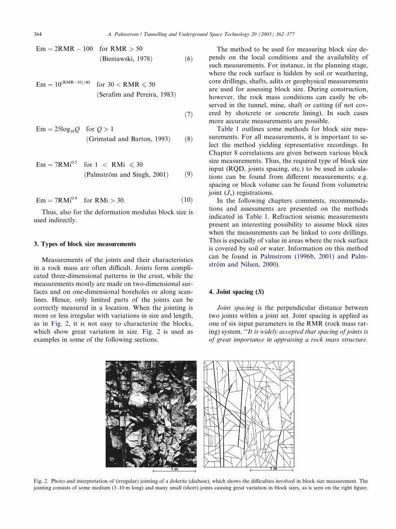
correctly measured in a location. When the jointing ismore or less irregular with variations in size and length,

as in Fig. 2, it is not easy to characterize the blocks,

which show great variation in size. Fig. 2 is used as

examples in some of the following sections.

Fig. 2. Photo and interpretation of (irregular) jointing of a dolerite (diabase

jointing consists of some medium (3–10 m long) and many small (short) join

The method to be used for measuring block size de-

pends on the local conditions and the availability of

such measurements. For instance, in the planning stage,

where the rock surface is hidden by soil or weathering,

core drillings, shafts, adits or geophysical measurements

are used for assessing block size. During construction,however, the rock mass conditions can easily be ob-

served in the tunnel, mine, shaft or cutting (if not cov-

ered by shotcrete or concrete lining). In such cases

more accurate measurements are possible.

Table 1 outlines some methods for block size mea-

surements. For all measurements, it is important to se-

lect the method yielding representative recordings. In

Chapter 8 correlations are given between various blocksize measurements. Thus, the required type of block size

input (RQD, joints spacing, etc.) to be used in calcula-

tions can be found from different measurements; e.g.

spacing or block volume can be found from volumetric

joint (Jv) registrations.

In the following chapters comments, recommenda-

tions and assessments are presented on the methods

indicated in Table 1. Refraction seismic measurementspresent an interesting possibility to assume block sizes

when the measurements can be linked to core drillings.

This is especially of value in areas where the rock surface

is covered by soil or water. Information on this method

can be found in Palmstrom (1996b, 2001) and Palm-

strom and Nilsen, 2000).

4. Joint spacing (S)

Joint spacing is the perpendicular distance between

two joints within a joint set. Joint spacing is applied asone of six input parameters in the RMR (rock mass rat-

ing) system. ‘‘It is widely accepted that spacing of joints is

of great importance in appraising a rock mass structure.

), which shows the difficulties involved in block size measurement. The

ts causing great variation in block sizes, as is seen on the right figure.

able 1

ome main methods for measuring block size

easurements in rock surfaces Measurements on drill cores Refraction seismic measurements

lock size (volume of block) (Vb) Rock quality designation (RQD) Sound velocity of rock massesa

olumetric joint count (Jv) Fracture frequencya

oint spacing (S) Joint intercepta

eighted joint density (wJd) Weighted joint density (wJd)

ock quality designation (RQD)b Block volume (Vb)c

a Not described in paper.b Estimated from scan line measurements.c In some sections with crushed rock.


T

S

M

B

V

J

W

R

set 1

join

t set

1

set 2

set 3

s1 s2s3 s4

s5 s6

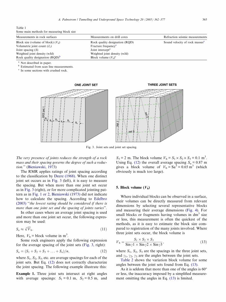
ONE JOINT SET THREE JOINT SETS

Fig. 3. Joint sets and joint set spacing.

The very presence of joints reduces the strength of a rock

mass and their spacing governs the degree of such a reduc-

tion.’’ (Bieniawski, 1973)

The RMR applies ratings of joint spacing according

to the classification by Deere (1968). When one distinct

joint set occurs as in Fig. 3 (left), it is easy to measure

the spacing. But when more than one joint set occur

as in Fig. 3 (right), or for more complicated jointing pat-tern as in Fig. 1 or 2, Bieniawski (1973) did not indicate

how to calculate the spacing. According to Edelbro

(2003) ‘‘the lowest rating should be considered if there is

more than one joint set and the spacing of joints varies’’.

In other cases where an average joint spacing is used

and more than one joint set occur, the following expres-

sion may be used:

Sa �ffiffiffiffiV3

pb: ð11Þ

Here, Vb = block volume in m3.

Some rock engineers apply the following expression

for the average spacing of the joint sets (Fig. 3, right):

Sa ¼ ðS1 þ S2 þ S3 þ . . .þ SnÞ=n; ð12Þwhere S1, S2, S3, etc. are average spacings for each of the

joint sets. But Eq. (12) does not correctly characterize

the joint spacing. The following example illustrate this:

Example 1. Three joint sets intersect at right angles

with average spacings: S1 = 0.1 m, S2 = 0.5 m, and

S3 = 2 m. The block volume Vb = S1 · S2 · S3 = 0.1 m3.

Using Eq. (12) the overall average spacing Sa = 0.87 m

gives a block volume of Vb = Sa3 = 0.65 m3 (which

obviously is much too large).

5. Block volume (Vb)

Where individual blocks can be observed in a surface,

their volumes can be directly measured from relevant

dimensions by selecting several representative blocks

and measuring their average dimensions (Fig. 4). Forsmall blocks or fragments having volumes in dm3 size

or less, this measurement is often the quickest of the

methods, as it is easy to estimate the block size com-

pared to registration of the many joints involved. Where

three joint sets occur, the block volume is

V b ¼S1 � S2 � S3

Sinc1� Sinc2� Sinc3; ð13Þ

where S1, S2, S3 are the spacings in the three joint sets,

and c1, c2, c3 are the angles between the joint sets.

Table 2 shows the variation block volume for some

angles between the joint sets found from Eq. (13).

As it is seldom that more than one of the angles is 60�or less, the inaccuracy imposed by a simplified measure-

ment omitting the angles in Eq. (13) is limited.

1 m

Vb = 0.05dm3

Vb = 0.05m3

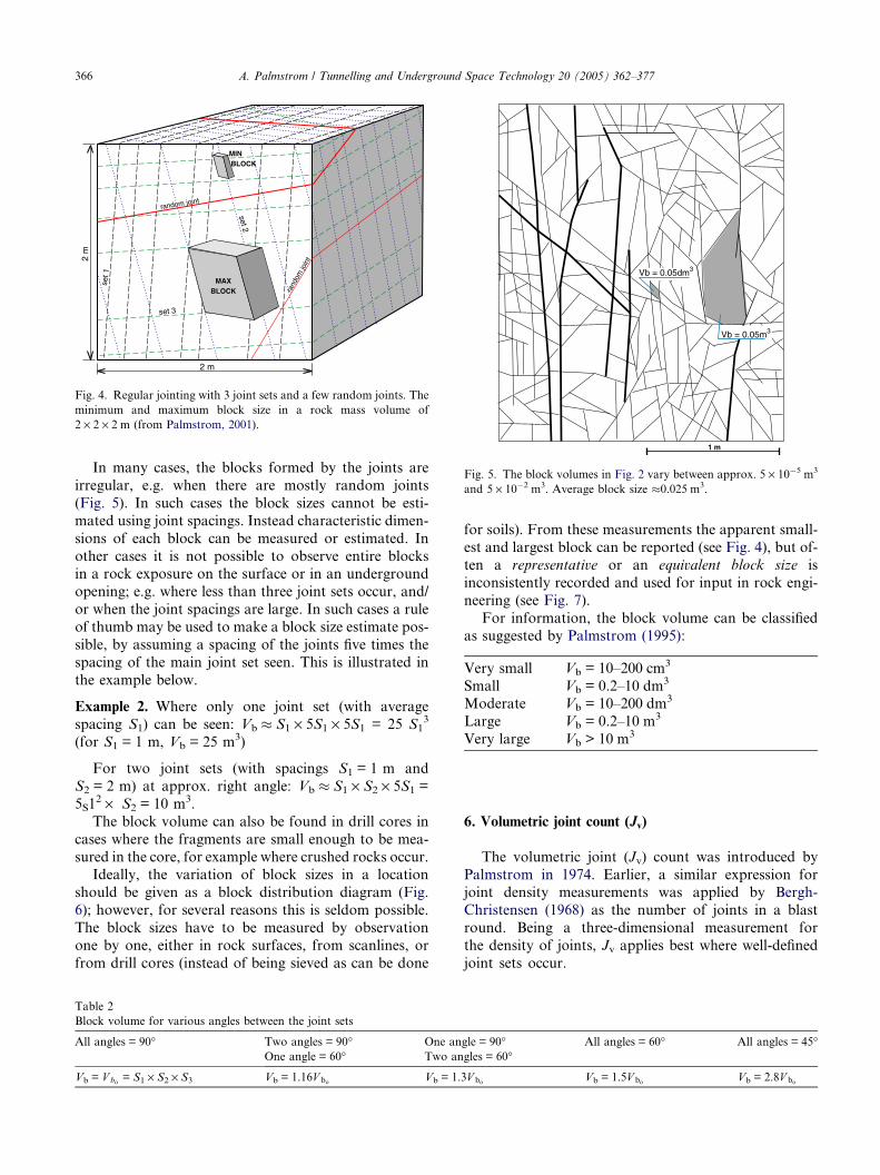
Fig. 5. The block volumes in Fig. 2 vary between approx. 5 · 10�5 m3

and 5 · 10�2 m3. Average block size �0.025 m3.

2 m

2 m

set 1

set 2

set 3

MAXBLOCK

MINBLOCK

random joint

rand

om jo

int

Fig. 4. Regular jointing with 3 joint sets and a few random joints. The

minimum and maximum block size in a rock mass volume of

2 · 2 · 2 m (from Palmstrom, 2001).


In many cases, the blocks formed by the joints are

irregular, e.g. when there are mostly random joints

(Fig. 5). In such cases the block sizes cannot be esti-

mated using joint spacings. Instead characteristic dimen-

sions of each block can be measured or estimated. In

other cases it is not possible to observe entire blocksin a rock exposure on the surface or in an underground

opening; e.g. where less than three joint sets occur, and/

or when the joint spacings are large. In such cases a rule

of thumb may be used to make a block size estimate pos-

sible, by assuming a spacing of the joints five times the

spacing of the main joint set seen. This is illustrated in

the example below.

Example 2. Where only one joint set (with average

spacing S1) can be seen: Vb � S1 · 5S1 · 5S1 = 25 S13

(for S1 = 1 m, Vb = 25 m3)

For two joint sets (with spacings S1 = 1 m and

S2 = 2 m) at approx. right angle: Vb � S1 · S2 · 5S1 =

5S12 · S2 = 10 m3.

The block volume can also be found in drill cores in

cases where the fragments are small enough to be mea-

sured in the core, for example where crushed rocks occur.Ideally, the variation of block sizes in a location

should be given as a block distribution diagram (Fig.

6); however, for several reasons this is seldom possible.

The block sizes have to be measured by observation

one by one, either in rock surfaces, from scanlines, or

from drill cores (instead of being sieved as can be done

Table 2

Block volume for various angles between the joint sets

All angles = 90� Two angles = 90� One an

One angle = 60� Two an

Vb = V bo = S1 · S2 · S3 Vb = 1.16V bo Vb = 1.

for soils). From these measurements the apparent small-

est and largest block can be reported (see Fig. 4), but of-

ten a representative or an equivalent block size is

inconsistently recorded and used for input in rock engi-

neering (see Fig. 7).

For information, the block volume can be classified

as suggested by Palmstrom (1995):

Very small

gle = 90�gles = 60�

3V bo

Vb = 10–200 cm3

All angles = 60�

Vb = 1.5V bo

All ang

Vb = 2.

les = 45

8V bo

Small
Vb = 0.2–10 dm3
Moderate
Vb = 10–200 dm3
Large
Vb = 0.2–10 m3
Very large
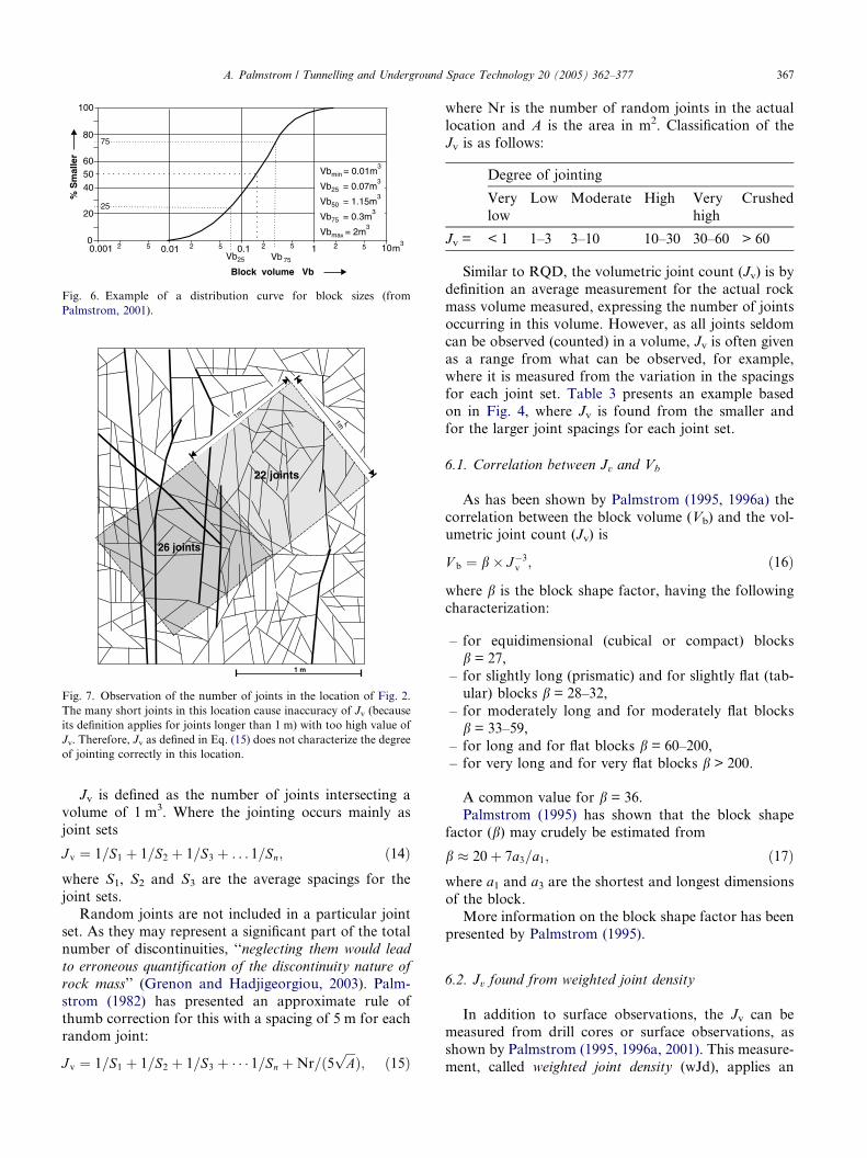
Vb > 10 m3
6. Volumetric joint count (Jv)

The volumetric joint (Jv) count was introduced by

Palmstrom in 1974. Earlier, a similar expression forjoint density measurements was applied by Bergh-

Christensen (1968) as the number of joints in a blast

round. Being a three-dimensional measurement for

the density of joints, Jv applies best where well-defined

joint sets occur.

�

1 m

26 joints

22 joints

1m

1m

Fig. 7. Observation of the number of joints in the location of Fig. 2.

The many short joints in this location cause inaccuracy of Jv (because

its definition applies for joints longer than 1 m) with too high value of

Jv. Therefore, Jv as defined in Eq. (15) does not characterize the degree

of jointing correctly in this location.

Block volume Vb

% S

mal

ler

0.001 0.01 0.1 1 10m30

20

40

60

80

100

2 5 2 5 2 5 2 5

Vb = 0.01m

Vb = 0.07m

Vb = 1.15m

Vb = 0.3m

Vb = 2m

min

25

50

75

max

3

3

3

3

3

50

Vb25 Vb 75

75

25

Fig. 6. Example of a distribution curve for block sizes (from

Palmstrom, 2001).


Jv is defined as the number of joints intersecting a

volume of 1 m3. Where the jointing occurs mainly as

joint sets

J v ¼ 1=S1 þ 1=S2 þ 1=S3 þ . . . 1=Sn; ð14Þwhere S1, S2 and S3 are the average spacings for the

joint sets.

Random joints are not included in a particular joint

set. As they may represent a significant part of the total

number of discontinuities, ‘‘neglecting them would lead

to erroneous quantification of the discontinuity nature of

rock mass’’ (Grenon and Hadjigeorgiou, 2003). Palm-

strom (1982) has presented an approximate rule ofthumb correction for this with a spacing of 5 m for each

random joint:

J v ¼ 1=S1 þ 1=S2 þ 1=S3 þ � � � 1=Sn þNr=ð5ffiffiffiA

pÞ; ð15Þ

where Nr is the number of random joints in the actual

location and A is the area in m2. Classification of the

Jv is as follows:

Degree of jointing

Very

low

Low
Moderate High Very
high

Crushed

Jv =
< 1 1–3 3–10 10–30 30–60 > 60
Similar to RQD, the volumetric joint count (Jv) is by

definition an average measurement for the actual rock

mass volume measured, expressing the number of joints

occurring in this volume. However, as all joints seldom

can be observed (counted) in a volume, Jv is often given

as a range from what can be observed, for example,

where it is measured from the variation in the spacingsfor each joint set. Table 3 presents an example based

on in Fig. 4, where Jv is found from the smaller and

for the larger joint spacings for each joint set.

6.1. Correlation between Jv and Vb

As has been shown by Palmstrom (1995, 1996a) the

correlation between the block volume (Vb) and the vol-umetric joint count (Jv) is

V b ¼ b� J�3v ; ð16Þ

where b is the block shape factor, having the following

characterization:

– for equidimensional (cubical or compact) blocks

b = 27,

– for slightly long (prismatic) and for slightly flat (tab-

ular) blocks b = 28–32,

– for moderately long and for moderately flat blocks

b = 33–59,

– for long and for flat blocks b = 60–200,

– for very long and for very flat blocks b > 200.

A common value for b = 36.

Palmstrom (1995) has shown that the block shape

factor (b) may crudely be estimated from

b � 20þ 7a3=a1; ð17Þwhere a1 and a3 are the shortest and longest dimensions

of the block.

More information on the block shape factor has been

presented by Palmstrom (1995).

6.2. Jv found from weighted joint density

In addition to surface observations, the Jv can be

measured from drill cores or surface observations, as

shown by Palmstrom (1995, 1996a, 2001). This measure-

ment, called weighted joint density (wJd), applies an

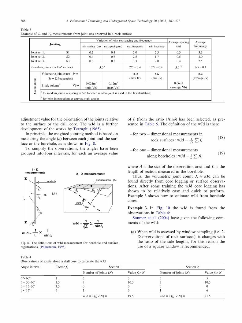
Table 3

Example of Jv and Vb measurements from joint sets observed in a rock surface

min spacing (m) max spacing (m) max frequency min frequency

0.2 0.4 5.0 2.5 0.3 3.30.4 0.6 2.5 1.7 0.5 2.00.3 0.5 3.3 2.0 0.4 2.5

2/5 = 0.4 2/5 = 0.4 5.0 *) 2/5 = 0.4

Volumetric joint count Jv =

(Jv = Σ frequencies)

Block volumeb Vb =0.024m3

(min Vb)0.12m3

(max Vb)0.06m³

(average Vb) a for random joints, a spacing of 5m for each random joint is used in the Jv calculation; C

alcu

lati

ons

b for joint intersections at approx. right angles

11.2 (max Jv)

6.6 (min Jv)

8.2 (average Jv)

5.0 a

Joint set 1, S1 Joint set 2, S2 Joint set 3, S3

2 random joints (in 1m² surface)

JointingVariation of joint set spacing and frequency Average spacing

(m)Average

frequency


adjustment value for the orientation of the joints relative

to the surface or the drill core. The wJd is a further

development of the works by Terzaghi (1965).

In principle, the weighted jointing method is based on

measuring the angle (d) between each joint and the sur-

face or the borehole, as is shown in Fig. 8.

To simplify the observations, the angles have been

grouped into four intervals, for each an average value

Table 4

Observations of joints along a drill core to calculate the wJd

Angle interval Factor fi Section 1

Number of joints (N)

d > 60� 1 3

d = 30–60� 1.5 7

d = 15–30� 3.5 0

d < 15� 6 1

wJd = R(fi · N) =

1

2

3

4

L

wJd =

wJd = 1

1sin i

sin i

1

1

L

A

1 3 2

1 - Dmeasurements 2 - D measurements

surface area (A)borehole

joint

joint

Fig. 8. The definitions of wJd measurement for borehole and surface

registrations. (Palmstrom, 1995).

of fi (from the ratio 1/sind) has been selected, as pre-

sented in Table 5. The definition of the wJd is then:

�for two� dimensional measurements in

rock surfaces : wJd ¼ 1ffiffiA

pP

fi;ð18Þ

�for one� dimensional measurements

along boreholes : wJd ¼ 1L

Pfi;

ð19Þ

where A is the size of the observation area and L is the

length of section measured in the borehole.

Thus, the volumetric joint count Jv � wJd can be

found directly from core logging or surface observa-

tions. After some training the wJd core logging has

shown to be relatively easy and quick to perform.Example 3 shows how to estimate wJd from borehole

cores.

Example 3. In Fig. 10 the wJd is found from the

observations in Table 4:

Sonmez et al. (2004) have given the following com-

ments of the wJd:

(a) When wJd is assessed by window sampling (i.e. 2-

D observations of rock surfaces), it changes with

the ratio of the side lengths; for this reason the

use of a square window is recommended.

Section 2

Value fi · N Number of joints (N) Value fi · N

3 5 5

10.5 7 10.5

0 0 0

6 1 6

19.5 wJd = R(fi · N) = 21.5

L = 38cm

L = 17cm

L = 0no pieces > 10cm

L = 20cm

L = 35cm

drilling break

Total length of core run = 200cm

200c

m

RQD = 0 -25% very poorRQD = 25 - 50 % poorRQD = 50 - 75% fairRQD = 75 - 90% goodRQD = 90 - 100% excellent

Table 5

Angle intervals and ratings of the factor fi in each interval

Angle interval (between joint

and borehole or surface)

1/sind Chosen rating of

the factor fi

d > 60� < 1.16 1

d = 30–60� 1.16–1.99 1.5

d = 15–30� 2–3.86 3.5

d < 15� > 3.86 6


(b) The joints nearly parallel to the observation sur-

face are not well represented in the sampling area.

Also the joints nearly parallel to the borehole axis

are not sampled. Therefore, the wJd will be

conservative.

(c) A minimum area required for the determination

has to be defined.

(d) The angle d between the joint surface and the bore-

hole axis has to be the maximum, otherwise, the

apparent joint spacing is considered instead of

the true spacing.

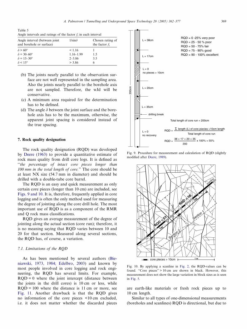
L = 0no recovery

RQD =

RQD =

length (L) of core piecies >10cm length

Total length of core run

38 + 17 + 20 + 35

200x 100% = 55%

Fig. 9. Procedure for measurement and calculation of RQD (slightly

modified after Deere, 1989).

1 m

scanlin

e

RQD = 58

RQD = 53

core pieces > 10cm

1m

1m

Section 1

Section 2

Fig. 10. By applying a scanline in Fig. 2, the RQD-values can be

found. ‘‘Core pieces’’ > 10 cm are shown in black. However, this

measurement does not show the large variation in block sizes as is seen

in Fig. 5.

7. Rock quality designation

The rock quality designation (RQD) was developed

by Deere (1963) to provide a quantitative estimate of

rock mass quality from drill core logs. It is defined as

‘‘the percentage of intact core pieces longer than

100 mm in the total length of core.’’ The core should be

at least NX size (54.7 mm in diameter) and should bedrilled with a double-tube core barrel.

The RQD is an easy and quick measurement as only

certain core pieces (longer than 10 cm) are included, see

Figs. 9 and 10. It is, therefore, frequently applied in core

logging and is often the only method used for measuring

the degree of jointing along the core drill hole. The most

important use of RQD is as a component of the RMR

and Q rock mass classifications.RQD gives an average measurement of the degree of

jointing along the actual section (core run); therefore, it

is no meaning saying that RQD varies between 10 and

20 for that section. Measured along several sections,

the RQD has, of course, a variation.

7.1. Limitations of the RQD

As has been mentioned by several authors (Bie-

niawski, 1973, 1984; Edelbro, 2003) and known by

most people involved in core logging and rock engi-

neering, the RQD has several limits. For example,

RQD = 0 where the joint intercept (distance between

the joints in the drill cores) is 10 cm or less, while

RQD = 100 where the distance is 11 cm or more, see

Fig. 11. Another drawback is that the RQD givesno information of the core pieces <10 cm excluded,

i.e. it does not matter whether the discarded pieces

are earth-like materials or fresh rock pieces up to10 cm length.

Similar to all types of one-dimensional measurements

(boreholes and scanlines) RQD is directional, but due to

S2 = 11cm S2 = 11cm S2 = 11cm

S1 = 9cm S1 = 9cm S1 = 9cmS3 = 15cm S3 = 15cm S3 = 15cm

Jv = 1/0.09 + 1/0.11 + 1/0.15 = 27 Jv = 1/0.09 + 1/0.11 + 1/0.15 = 27 Jv = 1/0.09 + 1/0.11 + 1/0.15 = 27

RQ

D =

0

RQD = 100

RQD = 100

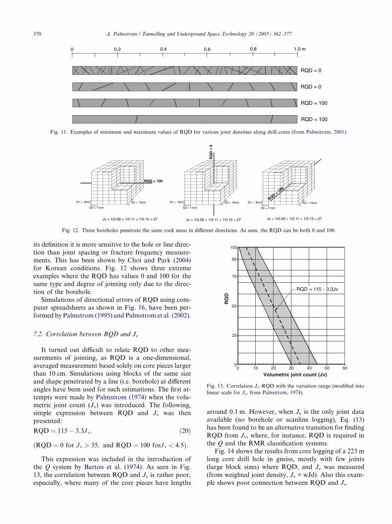
Fig. 12. Three boreholes penetrate the same rock mass in different directions. As seen, the RQD can be both 0 and 100.

50

75

90

100

RQ

D

RQD = 115 - 3.3Jv

0.2 0.4 0.60

RQD = 0

RQD = 0

RQD = 100

0.8 1.0 m

RQD = 100

Fig. 11. Examples of minimum and maximum values of RQD for various joint densities along drill cores (from Palmstrom, 2001).


its definition it is more sensitive to the hole or line direc-

tion than joint spacing or fracture frequency measure-

ments. This has been shown by Choi and Park (2004)

for Korean conditions. Fig. 12 shows three extreme

examples where the RQD has values 0 and 100 for the

same type and degree of jointing only due to the direc-

tion of the borehole.

Simulations of directional errors of RQD using com-puter spreadsheets as shown in Fig. 16, have been per-

formed by Palmstrom (1995) and Palmstrom et al. (2002).

0 10 20 30 40 50 600

25

Volumetric joint count (Jv)

Fig. 13. Correlation Jv–RQD with the variation range (modified into

linear scale for Jv, from Palmstrom, 1974).

7.2. Correlation between RQD and Jv

It turned out difficult to relate RQD to other mea-

surements of jointing, as RQD is a one-dimensional,

averaged measurement based solely on core pieces largerthan 10 cm. Simulations using blocks of the same size

and shape penetrated by a line (i.e. borehole) at different

angles have been used for such estimations. The first at-

tempts were made by Palmstrom (1974) when the volu-

metric joint count (Jv) was introduced. The following,

simple expression between RQD and Jv was then

presented:

RQD ¼ 115� 3:3J v; ð20Þ

ðRQD ¼ 0 for J v > 35; and RQD ¼ 100 forJ v < 4:5Þ:

This expression was included in the introduction of

the Q system by Barton et al. (1974). As seen in Fig.13, the correlation between RQD and Jv is rather poor,

especially, where many of the core pieces have lengths

around 0.1 m. However, when Jv is the only joint data

available (no borehole or scanline logging), Eq. (13)

has been found to be an alternative transition for finding

RQD from Jv, where, for instance, RQD is required in

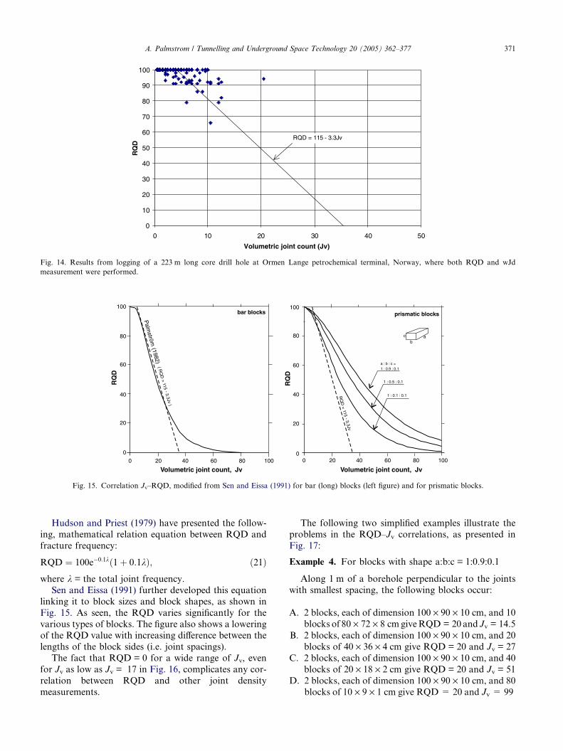
the Q and the RMR classification systems.Fig. 14 shows the results from core logging of a 223 m

long core drill hole in gneiss, mostly with few joints

(large block sizes) where RQD, and Jv was measured

(from weighted joint density, Jv = wJd). Also this exam-

ple shows poor connection between RQD and Jv.

Volumetric joint count, JvVolumetric joint count, Jv

prismatic blocksbar blocks

a : b : c =1 : 0.9 : 0.1

1 : 0.5 : 0.1

1 : 0.1 : 0.1RQ

D=

115-

3.3Jv

( RQ

D=

115- 3.3Jv

)

100

80

60

40

20

0

100

80

60

40

20

00 20 40 60 80 100 0 20 40 60 80 100

RQ

D

RQ

D

Palm

ström(1982)

ab

c

Fig. 15. Correlation Jv–RQD, modified from Sen and Eissa (1991) for bar (long) blocks (left figure) and for prismatic blocks.

0

10

20

30

40

50

60

70

80

90

100

0 10 20 30 40

Volumetric joint count (Jv)

RQ

D

50

RQD = 115 - 3.3Jv

Fig. 14. Results from logging of a 223 m long core drill hole at Ormen Lange petrochemical terminal, Norway, where both RQD and wJd

measurement were performed.


Hudson and Priest (1979) have presented the follow-

ing, mathematical relation equation between RQD and

fracture frequency:

RQD ¼ 100e�0:1kð1þ 0:1kÞ; ð21Þwhere k = the total joint frequency.

Sen and Eissa (1991) further developed this equation

linking it to block sizes and block shapes, as shown in

Fig. 15. As seen, the RQD varies significantly for the

various types of blocks. The figure also shows a loweringof the RQD value with increasing difference between the

lengths of the block sides (i.e. joint spacings).

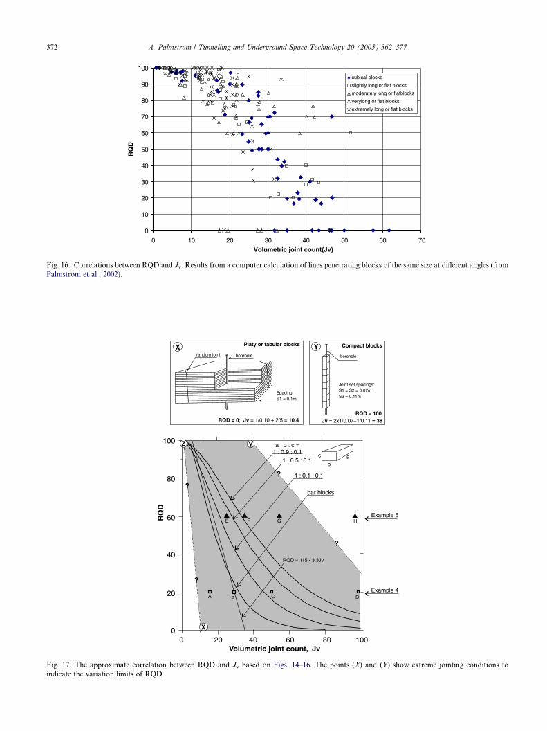
The fact that RQD = 0 for a wide range of Jv, even

for Jv as low as Jv = 17 in Fig. 16, complicates any cor-

relation between RQD and other joint density

measurements.

The following two simplified examples illustrate the

problems in the RQD–Jv correlations, as presented in

Fig. 17:

Example 4. For blocks with shape a:b:c = 1:0.9:0.1

Along 1 m of a borehole perpendicular to the jointswith smallest spacing, the following blocks occur:

A. 2 blocks, each of dimension 100 · 90 · 10 cm, and 10

blocks of 80 · 72 · 8 cmgiveRQD = 20 and Jv = 14.5

B. 2 blocks, each of dimension 100 · 90 · 10 cm, and 20

blocks of 40 · 36 · 4 cm give RQD = 20 and Jv = 27

C. 2 blocks, each of dimension 100 · 90 · 10 cm, and 40


D. 2 blocks, each of dimension 100 · 90 · 10 cm, and 80blocks of 10 · 9 · 1 cm give RQD= 20 and Jv = 99

0

10

20

30

40

50

60

70

80

90

100

0 10 20 30 40 50 60Volumetric joint count(Jv)

RQ

D

70

cubical blocks

slightly long or flat blocks

moderately long or flatblocks

verylong or flat blocks

extremely long or flat blocks

Fig. 16. Correlations between RQD and Jv. Results from a computer calculation of lines penetrating blocks of the same size at different angles (from

Palmstrom et al., 2002).

Volumetric joint count, Jv

a : b : c =1 : 0.9 : 0.1

1 : 0.5 : 0.1

1 : 0.1 : 0.1

RQD = 115 - 3.3Jv

100

80

60

40

20

00 20 40 60 80 100

RQ

D

ab

c

bar blocks

?

?

?

?

; = 1/0.10 + 2/5 =RQD = 0 Jv 10.4

Spacing:S1 = 0.1m

borehole boreholerandom joint

Joint set spacings:S1 = S2 = 0.07mS3 = 0.11m

Jv = 38= 2x1/0.07+1/0.11

Platy or tabular blocks Compact blocks

RQD = 100

X Y

X

YZ

A B C D

E F G HExample 5

Example 4

Fig. 17. The approximate correlation between RQD and Jv based on Figs. 14–16. The points (X) and (Y) show extreme jointing conditions to

indicate the variation limits of RQD.



Example 5. For blocks with shape a:b:c = 1:0.1:0.1

Along 1 m of a borehole perpendicular to the joints withsmallest spacing, the following blocks occur:

E. 6 blocks of dimension 100 · 10 · 10cm, and 5 blocks

of 80 · 8 · 8 cm give RQD = 60 and Jv = 23

F. 6 blocks of dimension 100 · 10 · 10 cm, and 10


Volumetric joint count, Jv

RQ

D=

115

-3.3

Jv

100

80

60

40

20

0

0 20 40 60 80 100

RQ

D

?

?

? ?

RQ

D=

110

-2.5

Jv

assu

med e

xtrem

e lim

it

assum

ed

extre

me

limit

?

assumed common variation

Fig. 18. The probable common variation for RQD–Jv and suggested

equations.

G. 6 blocks of dimension 100 · 10 · 10 cm, and 20blocks of 20 · 2 · 2 cm give RQD = 60 and Jv = 55

H. 6 blocks of dimension 100 · 10 · 10 cm, and 40


Note that the jointing used in the examples above sel-

dom occur in situ, – especially the very thin prismatic

blocks of 1 cm thickness – but they are used here to indi-cate the problems in finding a correlation between Jvand RQD.

In order to estimate the limits in the correlation be-

tween RQD and Jv, the cases X and Y in Fig. 17 have

been included, where

– X presents the theoretical minimum of Jv (11) for

RQD = 0 (for tabular blocks with spacing

S1 = 10 cm and wide spacings for S2 and S3), and

– Y is the theoretical maximum of Jv (�38) for

RQD = 100 (for compact (cubical) blocks). The theo-

retical minimum (Z) of Jv is close to zero for very

large blocks.

As shown, the minimum value (X) of Jv for RQD = 0is lower than the maximum Jv value (Y) for RQD = 100

(which also is the case in Fig. 16). In the interval

Jv = 15–30 the RQD can have values of both 0 and

100 or in between. Thus, in this interval RQD may have

any value.

Both Figs. 16 and 17 show that RQD is an inaccurate

measure for the degree of jointing. As it is often easier to

measure the Jv in a rock surface than the RQD, RQD isfrequently found from measurements of Jv using Eq.

RQD = 90

1m

10cm

wJd = 4x1 + 2x6= 16

seam (filled joint)

7o

84o

66o

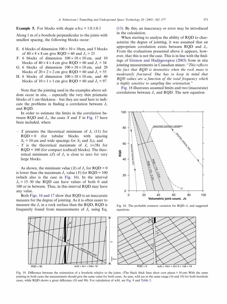
Fig. 19. Difference between the orientation of a borehole relative to the jo

jointing in both cases the measurement should give the same value for both c

cases, while RQD shows a great difference (10 and 90). For calculation of w

(13). By this, an inaccuracy or error may be introduced

in the calculation.

When starting to analyse the ability of RQD to char-

acterize the degree of jointing, it was assumed that an

appropriate correlation exists between RQD and Jv.

From the evaluations presented above it appears, how-ever, that this is not the case. This is in line with the find-

ings of Grenon and Hadjigeorgiou (2003) from in situ

jointing measurements in Canadian mines: ‘‘This reflects

the fact that RQD is insensitive when the rock mass is

moderately fractured. One has to keep in mind that

RQD values are a function of the total frequency which

is highly sensitive to sampling line orientation.’’

Fig. 18 illustrates assumed limits and two (inaccurate)correlations between Jv and RQD. The new equation

RQD = 9 wJd = 10x1 + 2x1.5 + 1x6 = 19

65o

40o

6o

ints. (The black thick lines show core pieces > 10 cm) With the same

ases. As seen, wJd are in the same range (16 and 19) for both borehole

Jd, see Fig. 8 and Table 5.

Table 6

The joint set number

Massive, no or few joints Jn = 0.5–1

One joint set 2

One joint set plus random 3

Two joint sets 4

Two joint sets plus random 6

Three joint sets 9

Three joint sets plus random 12

Four or more joint sets, heavily

jointed, ‘‘sugar-cube’’, etc.

15

Crushed rock, earth-like 20

0.1

1

10

100

0.0001 0.001 0.01 0.1 1 10 100

Block volume (m3)

RQ

D /

Jn

Fig. 21. Block volume RQD/Jn based on the same conditions as for

Fig. 16. Note that both axes are logarithmic (from Palmstrom et al.,

2002).


RQD ¼ 110� 2:5J v; ð22Þprobably gives a more appropriate average correlation

than the existing Eq. (20), which may be representativefor the more long or flat blocks, while Eq. (22) is better

for blocks of cubical (bar) shape. It has been chosen to

use Eq. (22) in the remaining part of this paper.

7.3. Comparison between RQD and wJd

The directional errors in one-dimensional measure-

ments in boreholes mentioned for the RQD measure-ment are partly compensated for in the wJd

measurements as indicated in Fig. 19, which shows an

example of RQD and wJd measurements for two bore-

holes in different directions to the same jointing. (Ide-

ally, the Jv as well as the RQD should have the same

value in the two measurements.)

Fig. 20 shows the results from logging of the degree of

jointing in drill cores by the Jv and by the RQD in prac-tice. Contrary to the RQD, the Jv shows variation in all

the three boreholes. Both Figs. 19 and 20 show the limi-

tation of RQD to correctly characterize the block size.

7.4. RQD/Jn as a measure for block size

The limits of RQD to characterize large blocks or

very small blocks may be reduced by introducing adjust-ments to it, as is done in the Q-system by the quotient

RQD/Jn, which uses ratings for the number of joint

set (Jn) as shown in Table 6.

The values of Jn varies from 0.5 to 20. According to

Barton et al. (1974), Grimstad and Barton (1993) and

several other papers presented by Barton, the ratio

RQD/Jn varies with the block size.

As RQD/Jn in Fig. 21 varies largely for the block vol-ume (Vb), this expression is an inaccurate characteriza-

tion of block size, though it extends the range the

block sizes compared to RQD alone (Hadjigeorgiou

0%

20%

40%

60%

80%

100%

crushed very high high moderate low very low

Jv > 60 Jv = 30 - 60 Jv = 10 - 30 Jv = 3 - 10 Jv = 1 - 3 Jv < 1

Volumetric joint count (joints/m3)

Dis

trib

uti

on

Hole 1Hole 2Hole 3

Logging by Jv

Fig. 20. Measurements of Jv (=wJd) and RQD in 3 borehole

et al., 1998) (another problem connected to this expres-

sion is that the number of joint sets is often prone to

wrong characterizations by the users. Many observers

apply all joint sets observed in a region, while Jn is the

number of joint sets at the actual location.)

Grenon and Hadjigeorgiou (2003) have from their in

situ investigations in Canadian mines also concluded

that the expression RQD/Jn is inaccurate in characteriz-ing block size.

0%

20%

40%

60%

80%

100%

very poor poor fair good very good excellent

RQD < 10 RQD = 10 -25

RQD = 26 -50

RQD = 51 -75

RQD = 76 -90

RQD > 90

RQD values

Dis

trib

uti

on

Hole 1Hole 2Hole 3

Logging by RQD

s with total length of 450 m in gneiss and amphibolite.


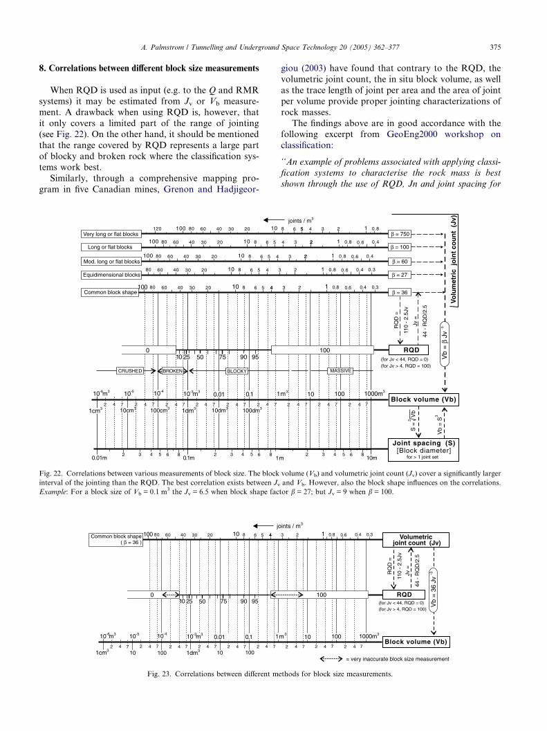
8. Correlations between different block size measurements

When RQD is used as input (e.g. to the Q and RMR

systems) it may be estimated from Jv or Vb measure-

ment. A drawback when using RQD is, however, that

it only covers a limited part of the range of jointing(see Fig. 22). On the other hand, it should be mentioned

that the range covered by RQD represents a large part

of blocky and broken rock where the classification sys-

tems work best.

Similarly, through a comprehensive mapping pro-

gram in five Canadian mines, Grenon and Hadjigeor-

10-510 m-6 3

80 60 40 30 20100 10 8 6 5 4 3 2 1 0.8 0.6 0.4 0.3

Block volume (Vb)

Joint spacing (S)[Block diameter]

10 m-3 3 1m3

1m

1000.1

0.1m

10

10m

Jv =

44 -

RQ

D/2

.5

RQ

D =

110

- 2.

5Jv

4

0.01

0.01m

Common block shape

0 100

1000m3

Vb

=Jv

-3

2510 75 90 95

10-4

50RQD

1cm3 10cm3 100cm3 1dm3 10dm3 100dm32 4 7 4 72 2 4 7 2 4 7 4 72 2 4 7 2 4 7 742 742

for > 1 joint set222 333 444 555 666 888

BROKENCRUSHED BLOCKY MASSIVE

80

80

80

80

60

60

60

60

40

40

40

40

30

30

30

30

20

20120

20

20

10

10100

100

100

10

10

8

8

8

8

6

6

6

6

5

5

5

5

4

4

4

4

3

3

3

3

2

2

2

2

1

1

1

1

0.8

0.8

0.8

0.8

0.6

0.6

0.6

0.4

0.4

0.4

0.3

V olu

met

ric

join

t co

un

t (

Jv)

joints / m3

= 100

Very long or flat blocks

Long or flat blocks

Mod. long or flat blocks

Equidimensional blocks

= 750

= 27

= 36

5

2

2= 60

(for Jv < 44, RQD = 0)(for Jv > 4, RQD = 100)

S =

V

b3

Vb

= S

3

Fig. 22. Correlations between various measurements of block size. The block volume (Vb) and volumetric joint count (Jv) cover a significantly larger

interval of the jointing than the RQD. The best correlation exists between Jv and Vb. However, also the block shape influences on the correlations.

Example: For a block size of Vb = 0.1 m3 the Jv = 6.5 when block shape factor b = 27; but Jv = 9 when b = 100.

10-510 m-6 3

80 60 40 30 20100 10 8 6 5 4 3 2 1 0.8 0.6 0.4 0.3

Block volume (Vb)10 m-3 3

joints / m3

1m3 1000.1 10

( = 36 )

Jv =

44 -

RQ

D/2

.5

RQ

D =

110

- 2.

5Jv

4

0.01

Common block shape

0 100

1000m3

Vb

= 3

6Jv

-3

2510 75 90 95

10-4

50

Volumetricjoint count (Jv)

RQD

1cm3 10 100 1dm3 10 1002 4 7 4 72 2 4 7 2 4 7 4 72 2 4 7 2 4 7 742 742

= very inaccurate block size measurement

(for Jv < 44, RQD = 0)(for Jv > 4, RQD = 100)

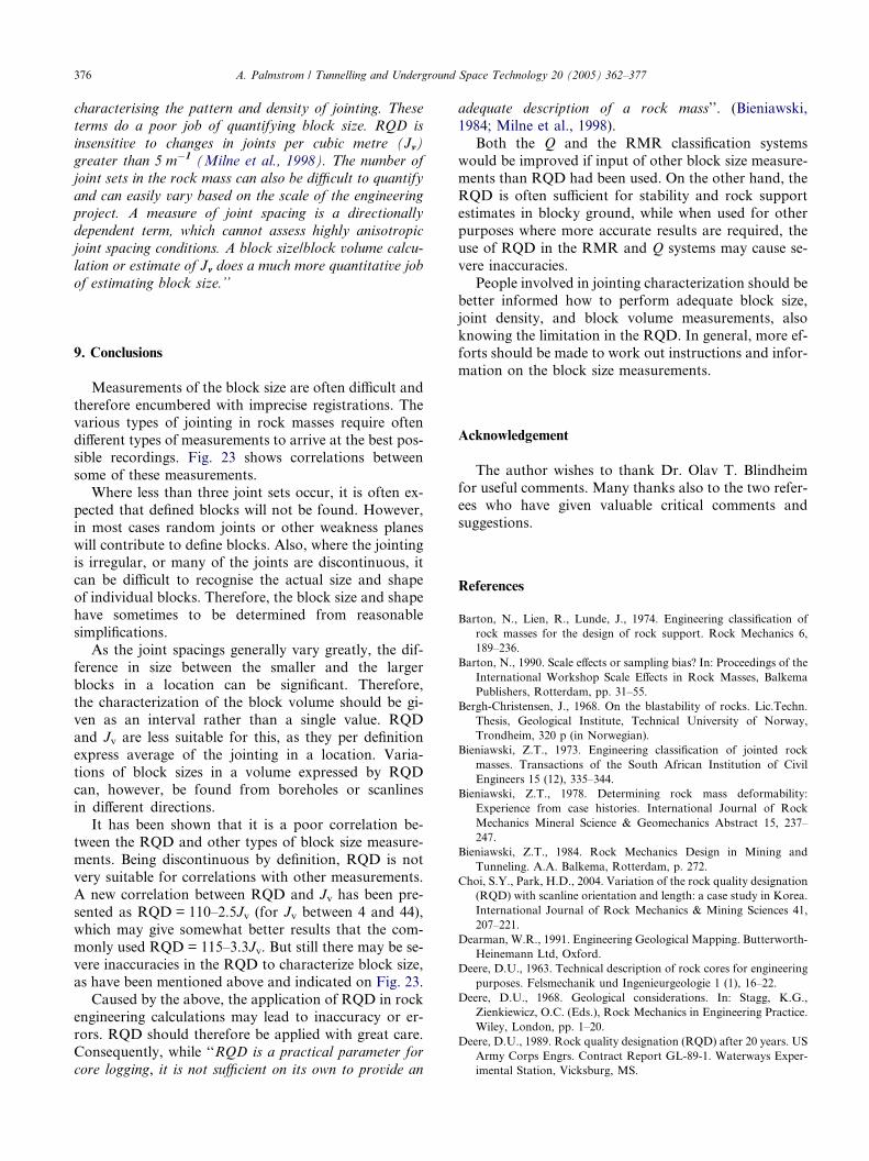
Fig. 23. Correlations between different methods for block size measurements.

giou (2003) have found that contrary to the RQD, the

volumetric joint count, the in situ block volume, as well

as the trace length of joint per area and the area of joint

per volume provide proper jointing characterizations of

rock masses.

The findings above are in good accordance with thefollowing excerpt from GeoEng2000 workshop on

classification:

‘‘An example of problems associated with applying classi-

fication systems to characterise the rock mass is best

shown through the use of RQD, Jn and joint spacing for


characterising the pattern and density of jointing. These

terms do a poor job of quantifying block size. RQD is

insensitive to changes in joints per cubic metre (Jv)

greater than 5 m�1 (Milne et al., 1998). The number of

joint sets in the rock mass can also be difficult to quantify

and can easily vary based on the scale of the engineering

project. A measure of joint spacing is a directionally

dependent term, which cannot assess highly anisotropic

joint spacing conditions. A block size/block volume calcu-

lation or estimate of Jv does a much more quantitative job

of estimating block size.’’

9. Conclusions

Measurements of the block size are often difficult and

therefore encumbered with imprecise registrations. Thevarious types of jointing in rock masses require often

different types of measurements to arrive at the best pos-

sible recordings. Fig. 23 shows correlations between

some of these measurements.

Where less than three joint sets occur, it is often ex-

pected that defined blocks will not be found. However,

in most cases random joints or other weakness planes

will contribute to define blocks. Also, where the jointingis irregular, or many of the joints are discontinuous, it

can be difficult to recognise the actual size and shape

of individual blocks. Therefore, the block size and shape

have sometimes to be determined from reasonable

simplifications.

As the joint spacings generally vary greatly, the dif-

ference in size between the smaller and the larger

blocks in a location can be significant. Therefore,the characterization of the block volume should be gi-

ven as an interval rather than a single value. RQD

and Jv are less suitable for this, as they per definition

express average of the jointing in a location. Varia-

tions of block sizes in a volume expressed by RQD

can, however, be found from boreholes or scanlines

in different directions.

It has been shown that it is a poor correlation be-tween the RQD and other types of block size measure-

ments. Being discontinuous by definition, RQD is not

very suitable for correlations with other measurements.

A new correlation between RQD and Jv has been pre-

sented as RQD = 110–2.5Jv (for Jv between 4 and 44),

which may give somewhat better results that the com-

monly used RQD = 115–3.3Jv. But still there may be se-

vere inaccuracies in the RQD to characterize block size,as have been mentioned above and indicated on Fig. 23.

Caused by the above, the application of RQD in rock

engineering calculations may lead to inaccuracy or er-

rors. RQD should therefore be applied with great care.

Consequently, while ‘‘RQD is a practical parameter for

core logging, it is not sufficient on its own to provide an

adequate description of a rock mass’’. (Bieniawski,

1984; Milne et al., 1998).

Both the Q and the RMR classification systems

would be improved if input of other block size measure-

ments than RQD had been used. On the other hand, the

RQD is often sufficient for stability and rock supportestimates in blocky ground, while when used for other

purposes where more accurate results are required, the

use of RQD in the RMR and Q systems may cause se-

vere inaccuracies.

People involved in jointing characterization should be

better informed how to perform adequate block size,

joint density, and block volume measurements, also

knowing the limitation in the RQD. In general, more ef-forts should be made to work out instructions and infor-

mation on the block size measurements.

Acknowledgement

The author wishes to thank Dr. Olav T. Blindheim

for useful comments. Many thanks also to the two refer-ees who have given valuable critical comments and

suggestions.

References

Barton, N., Lien, R., Lunde, J., 1974. Engineering classification of

rock masses for the design of rock support. Rock Mechanics 6,

189–236.

Barton, N., 1990. Scale effects or sampling bias? In: Proceedings of the

International Workshop Scale Effects in Rock Masses, Balkema

Publishers, Rotterdam, pp. 31–55.

Bergh-Christensen, J., 1968. On the blastability of rocks. Lic.Techn.

Thesis, Geological Institute, Technical University of Norway,

Trondheim, 320 p (in Norwegian).

Bieniawski, Z.T., 1973. Engineering classification of jointed rock

masses. Transactions of the South African Institution of Civil

Engineers 15 (12), 335–344.

Bieniawski, Z.T., 1978. Determining rock mass deformability:

Experience from case histories. International Journal of Rock

Mechanics Mineral Science & Geomechanics Abstract 15, 237–

247.

Bieniawski, Z.T., 1984. Rock Mechanics Design in Mining and

Tunneling. A.A. Balkema, Rotterdam, p. 272.

Choi, S.Y., Park, H.D., 2004. Variation of the rock quality designation

(RQD) with scanline orientation and length: a case study in Korea.

International Journal of Rock Mechanics & Mining Sciences 41,

207–221.

Dearman, W.R., 1991. Engineering Geological Mapping. Butterworth-

Heinemann Ltd, Oxford.

Deere, D.U., 1963. Technical description of rock cores for engineering

purposes. Felsmechanik und Ingenieurgeologie 1 (1), 16–22.

Deere, D.U., 1968. Geological considerations. In: Stagg, K.G.,

Zienkiewicz, O.C. (Eds.), Rock Mechanics in Engineering Practice.

Wiley, London, pp. 1–20.

Deere, D.U., 1989. Rock quality designation (RQD) after 20 years. US

Army Corps Engrs. Contract Report GL-89-1. Waterways Exper-

imental Station, Vicksburg, MS.


Edelbro, C., 2003. Rock mass strength – a review. Technical Report,

Lulea University of Technology, 132p.

GeoEng2000 workshop on classification systems, 2000. The reliability

of rock mass classification used in underground excavation and

support design. ISRM News 6(3), 2.

Goodman, R.E., 1993. Engineering Geology. Rock in Engineering

Construction. Wiley, New York, p. 385.

Grenon, M., Hadjigeorgiou, J., 2003. Evaluating discontinuity net-

work characterization tools through mining case studies. Soil Rock

America 2003, Boston 1, 137–142.

Grimstad, E., Barton, N., 1993. Updating the Q-system for NMT. In:

Proceedings of the International Symposium on Sprayed Concrete,

Fagernes, Norway 1993, Norwegian Concrete Association, Oslo,

20 pp.

Hadjigeorgiou, J., Grenon, M., Lessard, J.F., 1998. Defining in situ

block size. CIM Bulletin 91 (1020), 72–75.

Hoek, E., Brown, E.T., 1980. Empirical strength criterion for rock

masses. Journal of Geotechnical Engineering Division, ASCE

106(GT9), 1013–1035.

International Society for Rock Mechanics (ISRM), Commission on

standardization of laboratory and field tests, 1978. Suggested

methods for the quantitative description of discontinuities in rock

masses. Int. J. Rock Mech. Min. Sci. & Geomech. Abstr 15(6),

319–368.

Hoek, E., 1994. The challenge of input data for rock engineering.

Letter to the editor. ISRM, News Journal, 2, No. 2, 2 p.

Hudson, J.A., Priest, S.D., 1979. Discontinuities and rock mass

geometry. International Journal of Rock Mechanics Mining

Science & Geomechanics Abstr. 16, 339–362.

Milne, D., Hadjigeorgiou, J., Pakalnis, R., 1998. Rock mass charac-

terization for underground hard rock mines. Tunnelling and

Underground Space Technology 13 (4), 383–391.

Palmstrom, A., 1974. Characterization of jointing density and the

quality of rock masses. Internal report, A.B. Berdal, Norway, 26 p

(in Norwegian).

Palmstrom, A., 1982. The volumetric joint count – A useful and simple

measure of the degree of rock mass jointing. In: IAEG Congress,

New Delhi V.221-V.228.

Palmstrom, A., 1995. RMi – a rock mass characterization system for

rock engineering purposes. PhD thesis, University of Oslo,

Department of Geology, 400 pp.

Palmstrom, A., 1996a. The weighted joint density method leads to

improved characterization of jointing. In: International Conference

on Recent Advances in Tunnelling Technology, New Delhi, India,

6 p.

Palmstrom, A., 1996b. Application of seismic refraction survey in

assessment of jointing. In: International Conference on Recent

Advances in Tunnelling Technology, New Delhi, India, 9 p.

Palmstrom, A., Nilsen, B., 2000. Engineering Geology and Rock

Engineering. Handbook. Norwegian Rock and Soil Engineering

Association, p. 250.

Palmstrom, A., Singh, R., 2001. The deformation modulus of rock

masses – comparisons between in situ tests and indirect estimates.

Tunnelling and Underground Space Technology 16 (3), 115–131.

Palmstrom, A., 2001. Measurement and characterization of rock mass

jointing. In: Sharma, V.M., Saxena, K.R. (Eds.), In Situ Charac-

terization of Rocks. A.A. Balkema Publishers, pp. 49–97.

Palmstrom, A., Blindheim, O.T., Broch, E., 2002. The Q system –

possibilities and limitations. (in Norwegian) Norwegian annual

tunnelling conference on Fjellsprengningsteknikk/Bergmekanikk/

Geoteknikk, Oslo, pp. 41.1– 41.38.

Sen, Z., Eissa, E.A., 1991. Volumetric rock quality designation.

Journal of Geotechnical Engineering 117 (9), 1331–1346.

Serafim, J.L., Pereira, J.P., 1983. Consideration of the geomechanics

classification of Bieniawski. Proceedings of the International

Symposium on Engineering Geology and Underground Construc-

tions, 1133–1144.

Sonmez, H., Nefeslioglu, H.A., Gokceoglu, C., 2004. Determination of

wJd on rock exposures including wide spaced joints. Technical

note. Rock Mechanics and Rock Engineering 37 (5), 403–413.

Terzaghi, K., 1946. Rock defects and loads on tunnel supports. In:

Proctor, R.V., White, T.L., (Eds.), Rock tunneling with steel

supports, vol. 1, 17-99. Commercial Shearing and Stamping

Company, Youngstown, OH, pp. 5–153.

Terzaghi, R., 1965. Sources of error in joint surveys. Geotechnique 15,

287–304.

measurements of and correlations between block size and rock quality designation

Documents

input of block size

block size measurements

block size forms

block size andnation

various block sizemeasurements

rqd measurements

important input

patterns of jointing