Measurements of achromatic and chromatic contrastsensitivity functions for an extended range of adaptation

luminance

Kil Joong Kima, Rafal Mantiukb and Kyoung Ho Leea

aDept. of Radiation Applied Life Science, Seoul National Univ., 28 Youngon-dong,Chongno-gu, Seoul, 110-744, Korea;

bSchool of Computer Science, Bangor Univ., Dean Street, LL57 1UT, United Kingdom

ABSTRACT

Inspired by the ModelFest and ColorFest data sets, a contrast sensitivity function was measured for a wide rangeof adapting luminance levels. The measurements were motivated by the need to collect visual performance datafor natural viewing of static images at a broad range of luminance levels, such as can be found in the case of highdynamic range displays. The detection of sine-gratings with Gaussian envelope was measured for achromaticcolor axis (black to white), two chromatic axes (green to red and yellow-green to violet) and two mixed chromaticand achromatic axes (dark-green to light-pink, and dark yellow to light-blue). The background luminance variedfrom 0.02 to 200 cd/m2. The spatial frequency of the gratings varied from 0.125 to 16 cycles per degree. Morethan four observers participated in the experiments and they individually determined the detection thresholdfor each stimulus using at least 20 trials of the QUEST method. As compared to the popular CSF models, weobserved higher sensitivity drop for higher frequencies and significant differences in sensitivities in the luminancerange between 0.02 and 2 cd/m2. Our measurements for chromatic CSF show a significant drop in sensitivity withluminance, but little change in the shape of the CSF. The drop of sensitivity at high frequencies is significantlyweaker than reported in other studies and assumed in most chromatic CSF models.

Keywords: CSF, Contrast sensitivity function, high dynamic range, luminance masking, chromatic CSF

This version of the paper contains important corrections that had been made after the paper was published inthe SPIE digital library. The digital library versions has the data incorrectly scaled in Figs. 2–8.

1. INTRODUCTION

The contrast sensitivity functions (CSFs) are one of the main components of visual models and metrics. Mostmodels of CSFs were developed based on the data from numerous historical psychophysical experiments. How-ever, the models derived from such data suffer from several problems. Firstly, quite often the data from severaldistinct experiments had to be combined to cover the required range of spatial frequencies and luminance levels.Therefore, the data for different range of conditions could be inconsistent because it was measured for differentindividuals, different stimuli or experimental conditions. Secondly, the data was often collected using artificialviewing conditions, such as dilated and artificial pupils, flickering stimuli, narrowband light or the stimuli thatwas compensated for the effect of chromatic aberrations of the eye.1 Such conditions are unlikely to be found intypical viewing scenarios, where CSF models are meant to be used.

The ModelFest2 and ColorFest3 datasets were collected in an effort to build a general detection model of anaverage observer and to address the limitations of the historical data. However, those data sets have a majorlimitation that all stimuli were shown at a single background luminance.

In this study, we conducted the experiments for both achromatic and chromatic CSFs for a wide rangeof adapting luminance levels, inspired by the measurements made for the ModelFest and ColorFest data set.We created sine-grating stimuli for achromatic CSF (black to white) and two chromatic CSFs (green to red and

Further author information: (Send correspondence to K.J.K.)K.J.K.: E-mail: kil210@gmail.com, Telephone: 82 10 4146 4889

yellow-green to violet) and two mixed chromatic and achromatic CSFs (dark-green to light-pink, and dark yellowto light-blue) while varying the background luminance levels from 0.02 to 200 cd/m2. The frequency range ofthe sine gratings varied from 0.125 to 16 cpd (cycles per degree). More than four observers participated in theexperiments and they individually determined the detection threshold for each stimulus using 20 trials of QUESTmethod.4

The results of our achromatic CSF measurements, together with a model explaining the data, were reportedelsewhere.5 This paper extends the discussion of the data, reports the data for individual observers and alsopresents the results of the new measurements for chromatic, and mixed chromatic and achromatic CSF.

2. RELATED WORKS

2.1 Achromatic CSF

The achromatic CSFs have been measured in a number of studies. An excellent review of these measurementscan be found in Barten.6 One study that covered the largest range of conditions and is thus the closest to ourmeasurements, is that of Meeteren and Vos.7 The measurements extended a wide range of luminance from 0.0001to 10 cd/m2 and the range of frequencies from 0.5 to 30 cpd. Our measurements extend into higher luminancelevels (150 cd/m2), which are more relevant for photopic vision, and also lower frequencies, down to 0.125 cpd.Such low frequencies are necessary to observe and model the band-pass characteristic of CSF, especially for lowluminance levels. The field size of the stimuli used in the Meeteren and Vos experiment was relatively large,extending 17 x 11 deg. Such large fields pose problems when they need to be represented as images in visualmodels. Their measurements were collected for only 2 observers.

A number of analytical CSF models have been proposed in the literature to explain the collected data.However, the vast majority of these models accounted for the effect of frequency alone. The second factor thathas the highest effect on the detection threshold is luminance. The effect of luminance was modelled in twocomprehensive CSF models, one proposed by Barten6 and another by Daly.8 Both CSF models rely on complexanalytical formulas, which are fitted to the data reported in the literature. Barten’s model is a meticulouslyderived composition of more basic models contributing to the detection process. These include optical transferfunction and psychometric function. Barten’s model was shown to predict many historical CSF measurements.However, its main weakness is that it is valid only for photopic (cone-mediated) vision. Fewer details are knownabout the derivation of the Daly’s model and only the final formula is reported.8

2.2 Chromatic CSF

There have been several studies measuring chromatic CSFs,1,9–12 however we could not find the data that wouldcover the wide range of luminance levels. Similarly as in case of achromatic CSF, the conditions used for someof these measurements were not consistent with the goal of visual models and metrics. We briefly explain theprevious research on chromatic CSFs.

Green9 measured the CSFs at different luminance levels where coloured sine-grating was shown on a back-ground of different color. No effort was made to produce isoluminant patterns and hence the resulting CSFs had aband-pass shape typical for achromatic CSF. This is in contrast to modern chromatic CSF measurements, whichattempt to stimulate only chromatic mechanisms of the visual system. The viewing conditions were strictlycontrolled but were also atypical of the normal viewing: artificial and dilated pupil, monocular viewing, thestimuli was corrected for chromatic aberrations with lens.

Granger and Heurtley10 measured red-green chromatic CSF with yellow background at 85 trolands (27 cd/m2)over the range 0.125–20 cpd. They reported low-pass characteristic of the CSF, consistent with the data of vander Horst and Bouman.13 But they also observed that high-frequency patterns are seen as achromatic (blackto white), rather than color modulations. When the detection criterion was the recognition of color, a narrowerspatial frequency band-pass was measured. We observed the same phenomenon in our measurement, howeverwe used the detection as a criterion.

The chromatic CSFs from Mullen’s 1985 paper1 have been widely used in color visual models.14,15 However,this data is not representative as a model of an average observer. The experiment was designed to discard the

effect of chromatic aberration in the eye while such aberration actually happens when perceiving normal scenes.In addition, they measured the chromatic CSFs only at a single luminance level.

Hirai et al.12 measured achromatic spatio-velocity (SV) CSF at 100 cd/m2 and two chromatic SV-CSF at38.5 cd/m2 for red to green and at 12.2 cd/m2 for blue to yellow, all in the range 0.5–8 cpd. The data wasused to model chromatic spatio-velocity contrast sensitivity. The model was then used to extend the sCIELabquality metric16 to the temporal domain. Because of the application, the stimuli was observed in naturalconditions. Flicker photometry was used to find isoluminant chromatic axes. The data is quite consistent withour measurements, but it was measured for a single luminance level.

3. EXPERIMENT DESIGN

3.1 Stimuli

The stimuli design was inspired by the ModelFest and ColorFest data sets. The stimuli consisted of verticalsine-gratings attenuated by a Gaussian envelope. The standard deviation of the Gaussian was equal to 1.5 visualdegree for all stimuli except for the lowest frequency of 0.25 cpd for chromatic and mixed chromatic stimuli (C2,C3, C6 and C7), where the standard deviation was equal to 3 visual degrees. The background luminance variedfrom 0.02 to 200 cd/m2. The luminance levels were selected to make the best use of the colour gamut of thedisplay and to avoid luminance levels lower than 10 cd/m2, at which the color calibration was unreliable. Theluminance levels below 10 cd/m2 were achieved by wearing modified welding goggles in which the protective glasshad been replaced with neutral density filters (Kodak Wratten Gelatin) with either 1.0D, 2.0D densities, or bothfilters together to achieve 3.0D (1000 times light reduction). The frequency range of the sine gratings variedfrom 0.125 to 16 cpd for achromatic stimuli and from 0.25 to 8 for chromatic stimuli. Some combinations offrequencies and luminance levels were omitted from the measurements because they required producing stimuliof very high contrast that exceeded the color gamut of the display. Stimuli were observed with a natural pupil.The area of the screen outside the stimulus was set to the mean luminance level. The stimuli were created for fivecolor directions, black to white, red to green, yellow-green to violet, dark-green to light-pink, and dark-yellow tolight-blue, which are denoted as C1, C2, C3, C6, and C7 following the same convention as used in the ColorFestpaper.3 The detail of creation of the stimuli is described elsewhere.3

We found that the white-point reported for the Colorfest dataset appears very bluish. After convertingthe chromatic coordinates of the background color from the LMS to xyY color space, the white point has thecoordinates x = .285, y = .313 which result in a color that is even more bluish than the illuminant D75. To makethe color of the white point more consistent with the modern display neutral white, the von Kries transformwas used to bring the background colour of all images to the color of the illuminant D65 (Table 1, Figure 1).It can be expected that this change will have a minor effect on the results because the chromatic adaptationmechanism of the visual system is likely to compensate for the reference white color. However, this backgroundcolor change will affect the reported contrast values, as explained in Section 3.2.

In contrast to most CSF measurements, the stimuli were not modulated over time and the presentation timewas not limited. This is because our goal was to collect the data for visual models that would apply to staticimages. It could be argued that the data for steady-viewing without temporal flicker better corresponds to thecase when two complex images are compared side by side. To mask the onset of the stimuli, a white noise patternof high contrast was shown just before and after the stimuli was shown.

3.2 Contrast units

All data is reported in terms of sensitivity, S, which is defined as the inverse of the threshold contrast C:

S =1

C(1)

For better visualization, the sensitivity is plotted using log10 scale. The data for achromatic CSF is reported asa relative modulation of the sine-grating:

C =m

Lb(2)

Table 1. The L, M, S cone excitations of the endpoints (From color and To color) of the color directions and of thebackgound (D65) after correcting the white point of ColorFest paper.

ColordirectionBackground(D65) From color To colorL M S L M S L M S

C1(Black to white) 26.19 13.81 0.35 24.88 13.12 0.33 27.50 14.50 0.37C2(Green to red) 26.19 13.81 0.35 26.25 13.76 0.35 26.13 13.86 0.35C3(Y ellow − green to violet) 26.19 13.81 0.35 26.19 13.81 0.31 26.19 13.81 0.39C6(Dark − green to light− pink) 26.19 13.81 0.35 25.76 13.62 0.31 26.62 14.00 0.39C7(Dark − yellow to light− blue) 26.19 13.81 0.35 26.70 14.17 0.40 25.68 13.45 0.30

0.25 cpd

C1

0.5 cpd 1 cpd 2 cpd 4 cpd

C2

C3

C6

C7

Figure 1. A subset of the stimuli used in our experiment.

where m is the amplitude of the sine grating and Lb is the luminance of the background. For chromatic CSF,we follow the contrast definition used for the ColorFest study3 and compute it as:

C =1√3

√(∆L

L

)2

+

(∆M

M

)2

+

(∆S

S

)2

(3)

where ∆L|∆M |∆S are the modulations of the grating along L|M|S-dimensions of the LMS color space, andL|M |S are the LMS trichromatic color values of the background color.

The following transformation was used to convert from CIE 1931 Standard Observer color matching functionsto the LMS cone response color space:17 L

MS

=

0.15514 0.54312 −0.03286−0.15514 0.45684 0.03286

0 0 0.00801

· XYZ

. (4)

3.3 Display and viewing conditions

The experiments were run in two separate laboratories using two different displays: 26 NEC SpectraView 2690(in Bangor University) and 24” HP LP2480sz (in Seoul National University). Both are high quality, 1 920 x1 200 pixel resolution, LCD displays offering good color reproduction with a 10-bit LCD panel and RGB LEDbacklight. Additional two bits of bit-depth were simulated by spatio-temporal dithering, implemented on thegraphics card using fragment programs. This gave the effective bit-depth resolution of 12-bits, which is necessaryfor near-threshold detection experiments. Stimuli were observed from a fixed distance of 93 cm, which gave anangular resolution of 60 pixels per visual degree. Only for the lowest frequency of 0.25 cpd for C2, C3, C6and C7 we used much shorter viewing distance of 49 cm, which corresponds to the angular resolution of 32pixels per visual degree. The displays were calibrated using a spectro-radiometer. The calibration accountedfor the spectral emission characteristic of each display. The display white point was fixed at D65. The detail ofcalibration procedure is described in the subsequent section.

3.4 Display calibration

Since generating accurate luminance and color is crucial for the CSF experiments, extra care was taken tocalibrate the displays used in the experiments. To model the relation between pixel values and colorimetricvalues, we used the gamma-offset-gain (GOG)18 display model:XY

Z

= MRGB−>XY Z

RγrGγg

Bγb

+

XB

YBZB

(5)

where [X Y Z]′ are the trichromatic color values for the displayed color, MRGB→XY Z is the RGB → XY Ztransformation matrix, [RGB]′ are pixel values and γr, γg, γb are gamma values of each individual colorcomponent. [XB YB ZB ]′ is the color of the black level. The transform matrix, the black level and the gammavalues for each color channel were found by least-square fitting to the display measurements. The fit was goodfor both displays. Although a lookup table could potentially be more accurate than the gamma function weused, the measurement noise made the display response curve non-monotonic and therefore not suitable for alook-up table.

3.5 Experiment procedure

Seven observers participated in the measurements of the achromatic stimuli (C1: black to white) and six ob-servers participated in the measurements of the chromatic stimuli (C2 and C3). In case of C1, four observerscompleted the experiment for all luminance levels and three observers for luminance of 2 cd/m2 and higher. Themeasurements were repeated for selected observers or for those measurements that varied significantly from theaveraged results.

The detection threshold of each stimulus was determined through at least 20 trials of the QUEST method.4

In each trial, four-alternative-forced-choice (4AFC) method was used: four stimuli, of which three were referenceimages and only one was test image, were shown side-by-side on the same screen without restricting the presen-tation time. The observers were asked to choose which of the four stimulus contained the pattern. We found the4AFC method faster converging than 2AFC because of the lower probability of correct guesses. Based on theobserver’s response, the QUEST method was used to find the degree of contrast for the next trial. The degreeof contrast for the initial trial was determined using the method of adjustment, in which an observer was askedto adjust contrast of the shown pattern until it was barely visible. Each observer completed all the tests in 3-4sessions of 30-45 minutes each. Details on the QUEST are described in the subsequent section.

3.6 QUEST

A number of methods are available for estimating the threshold of a stimulus and they can be largely divided intotwo categories:19 constant-stimuli methods and adaptive procedures. In the constant-stimuli method, humanresponses for the visibility of a stimulus with different magnitudes (usually more than four or five) are collectedand then the threshold of the stimulus is inferred from the collected results. The magnitudes of the stimulus are

0.125 0.25 0.5 1 2 4 8 16−0.5

0

0.5

1

1.5

2

2.5

Observer: fldlo

g1

0 S

en

sitiv

ity

0.125 0.25 0.5 1 2 4 8 16−0.5

0

0.5

1

1.5

2

2.5

Observer: jpt

0.125 0.25 0.5 1 2 4 8 16−0.5

0

0.5

1

1.5

2

2.5

Observer: kjk

0.125 0.25 0.5 1 2 4 8 16−0.5

0

0.5

1

1.5

2

2.5

Observer: pfi

0.125 0.25 0.5 1 2 4 8 16−0.5

0

0.5

1

1.5

2

2.5

Observer: rfm

Spatial frequency [cpd]

log

10 S

en

sitiv

ity

0.125 0.25 0.5 1 2 4 8 16−0.5

0

0.5

1

1.5

2

2.5

Observer: tom

Spatial frequency [cpd]0.125 0.25 0.5 1 2 4 8 16

−0.5

0

0.5

1

1.5

2

2.5

Observer: vib

Spatial frequency [cpd]0.125 0.25 0.5 1 2 4 8 16

−0.5

0

0.5

1

1.5

2

2.5

Spatial frequency [cpd]

All participants

150 cd/m2

20 cd/m2

2 cd/m2

0.2 cd/m2

0.02 cd/m2

Figure 2. Measurements of the achromatic CSF (C1: black to white) for individual observers and averaged results acrossall observers (bottom-right plot). Different line colors denote different background luminance levels. If no error bar ispresent, only a single measurement (20-trials of the QUEST procedure) was made for that point. Otherwise, the error-bardenotes the standard deviation.

predefined to range from 0% to 100% visibility based on a prior knowledge derived from literature or a preliminaryexperiment. The adaptive procedures are based on the assumptions about the distribution of responses near thethreshold and an actual shape of the psychometric function. In the adaptive procedure, many trials are repeatedwhile varying the magnitude of the stimulus. The magnitude of a current trial is determined on the basis ofthe observer’s responses in previous trials. Based on the results of psychophysical experiments, these adaptiveprocedures are demonstrated to be more accurate and efficient than the constant-stimuli method20 given thesame number of trials. QUEST is an adaptive procedure. It has been widely used for estimating thresholdsin psychology fields.21–24 The QUEST algorithm assumes that the detection probability function of observerfollows a Weibull distribution. In our experiment, the stimuli magnitude was the degree of the contrast. QUESTadaptively determines the degree of contrast for the next trial based on the observer’s response for the currentcomparison of the reference and test stimuli. Our custom experiment code used the QUEST implementationfrom Psychtoolbox (version 3), which is a Matlab toolbox for creating psychophysical experiments.25

4. RESULTS

4.1 Achromatic CSF

Figure 2 shows the results of the achromatic CSF (C1: black to white) measurements for individual observersand averaged results across all observers. The average observer data, plotted in the rightmost bottom plot, showsa typical band-pass characteristic with the peak frequency shifting from 2.8 cpd at 150 cd/m2 to about 0.7 cpd at0.02 cd/m2. As luminance decreases, so does sensitivity. However, the sensitivity does not drop with luminancefor frequencies less than 1 cpd and the luminance range between 2 cd/m2 and 150 cd/m2. There is little differencein sensitivities between 20 cd/m2 and 150 cd/m2, which suggests that the Weber law is a good approximation ofthe visual system detection performance for higher luminance levels. The most unexpected observation is thatthe peak sensitivity for 20 cd/m2 exceeds the peak for 150 cd/m2 for the frequencies between 1.4 and 2.8 cpd,demonstrating that we can be more sensitive to lower luminance levels. Such a peak in sensitivity with increasing

0.125 0.25 0.5 1 2 4 8 16−0.5

0

0.5

1

1.5

2

2.5

Spatial frequency [cpd]

log

10 S

en

sitiv

ity

Compared with Daly’s CSF

150 cd/m2

20 cd/m2

2 cd/m2

0.2 cd/m2

0.02 cd/m2

0.125 0.25 0.5 1 2 4 8 16−0.5

0

0.5

1

1.5

2

2.5

Spatial frequency [cpd]

Compared with Barten’s CSF

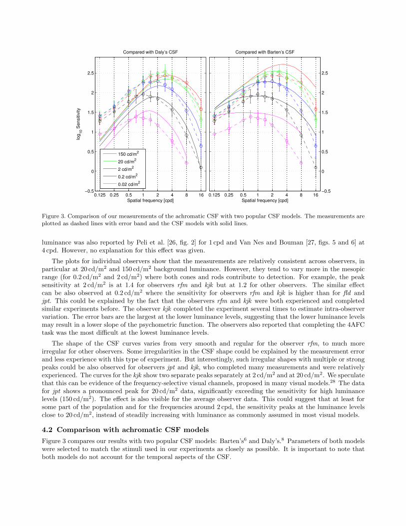
Figure 3. Comparison of our measurements of the achromatic CSF with two popular CSF models. The measurements areplotted as dashed lines with error band and the CSF models with solid lines.

luminance was also reported by Peli et al. [26, fig. 2] for 1 cpd and Van Nes and Bouman [27, figs. 5 and 6] at4 cpd. However, no explanation for this effect was given.

The plots for individual observers show that the measurements are relatively consistent across observers, inparticular at 20 cd/m2 and 150 cd/m2 background luminance. However, they tend to vary more in the mesopicrange (for 0.2 cd/m2 and 2 cd/m2) where both cones and rods contribute to detection. For example, the peaksensitivity at 2 cd/m2 is at 1.4 for observers rfm and kjk but at 1.2 for other observers. The similar effectcan be also observed at 0.2 cd/m2 where the sensitivity for observers rfm and kjk is higher than for fld andjpt. This could be explained by the fact that the observers rfm and kjk were both experienced and completedsimilar experiments before. The observer kjk completed the experiment several times to estimate intra-observervariation. The error bars are the largest at the lower luminance levels, suggesting that the lower luminance levelsmay result in a lower slope of the psychometric function. The observers also reported that completing the 4AFCtask was the most difficult at the lowest luminance levels.

The shape of the CSF curves varies from very smooth and regular for the observer rfm, to much moreirregular for other observers. Some irregularities in the CSF shape could be explained by the measurement errorand less experience with this type of experiment. But interestingly, such irregular shapes with multiple or strongpeaks could be also observed for observers jpt and kjk, who completed many measurements and were relativelyexperienced. The curves for the kjk show two separate peaks separately at 2 cd/m2 and at 20 cd/m2. We speculatethat this can be evidence of the frequency-selective visual channels, proposed in many visual models.28 The datafor jpt shows a pronounced peak for 20 cd/m2 data, significantly exceeding the sensitivity for high luminancelevels (150 cd/m2). The effect is also visible for the average observer data. This could suggest that at least forsome part of the population and for the frequencies around 2 cpd, the sensitivity peaks at the luminance levelsclose to 20 cd/m2, instead of steadily increasing with luminance as commonly assumed in most visual models.

4.2 Comparison with achromatic CSF models

Figure 3 compares our results with two popular CSF models: Barten’s6 and Daly’s.8 Parameters of both modelswere selected to match the stimuli used in our experiments as closely as possible. It is important to note thatboth models do not account for the temporal aspects of the CSF.

Daly’s CSF is plotted in the left plot of Figure 3 as the family of the band-pass contrast sensitivity functions.As the background luminance decreases, the sensitivity drops and the peak shifts towards lower frequencies,consistently with our results. However, Daly’s model also predicts much stronger drops in sensitivities for lowfrequencies, and much stronger shift in the peaks and lower sensitivity for 0.02 cd/m2. The differences aresignificant and we did not find a way to compensate for them by varying the parameters of the model.

The default set of parameters was used to plot Barten’s CSF model [6, p. 39] on the right of Figure 3. Themodel matches our data well for low frequencies. But the drop of sensitivity for high frequencies is smallerthan in the case of our data. Barten’s model also predicts flattening of the CSF with lower luminance levels,which results in much less pronounced peak of the sensitivity at low luminance. We could not observe thisbehavior in our data. The predicted sensitivities for lower luminance levels are also much lower than found inthe experiments. This is most likely because Barten’s model is valid for the photopic luminance range only andit was not meant to predict sensitivity for the luminance as low 0.2 or 0.02 cd/m2. The discrepancies of thismodel in the scotopic range are also reported in [6, p. 45,51].

The results show significant differences between both CSF models and our measured data. The differencesdo not necessarily indicate problems with the models, but rather that the data used for fitting these models wasmost likely measured for different stimuli than the one used in our experiments. For example, in our experimentthe size of the stimuli was kept constant regardless of the frequency. This resulted in a larger number of displayedsine-wave cycles for higher frequencies. But it is known that the number of cycles has a significant effect ondetection, especially for low frequencies.29 Some CSF measurements kept the number of cycles constant andvaried size, which could result in very different sensitivity results. Another significant difference was that thepresentation time was not limited and the stimuli were not modulated over time in our measurement (0-Hztemporal frequency), while the majority of CSF measurements are performed for temporarily modulated stimuli.The most important observation from these differences is that the shape of CSF depends on a much largernumber of parameters than spatial frequency and luminance and this fact must be considered when selecting aCSF model for a particular application. For example, the CSF meant for temporarily flickering Gabor patchesmay not be the most appropriate for predicting visibility thresholds in static images.

4.3 Chromatic CSF

The measurements of the chromaic CSF averaged over all observers are shown in Figure 4. The plots for thered-to-green (C2) and yellow-green-to-violet (C3) color axes show the low-pass characteric of the chromaticmechanism, also reported in other studies. However, band pass shapes are weakly shown for the photopic range(i.e., 40 cd/m2 and 200 cd/m2) for both C2 and C3. Such a moderate drop at low frequencies could be alsoobserved in the measurements of Granger and Heurtley [10, fig. 2], even though they used flicker photometry toensure isoluminance. The drop of sensitivity with increasing frequencies is moderate compared to the drop ofsensitivity with luminance. The sensitivities at 40 cd/m2 and 200 cd/m2 are almost identical, similarly as for theachromatic CSF. In contrast to achromatic CSF, there is little change in the shape of the CSF with decreasingluminance.

The dark-green to light-pink (C6) and dark-yellow to light-blue (C7) color axes are the mixture of chromaticand achromatic CSFs. The sensitivity curves show the predominantly low-pass characteristic of the chromaticmechanism, but also the shift of the sensitivity towards lower frequencies, which is typical for achromatic CSF.

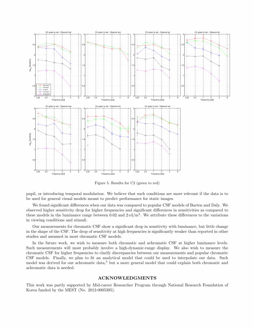
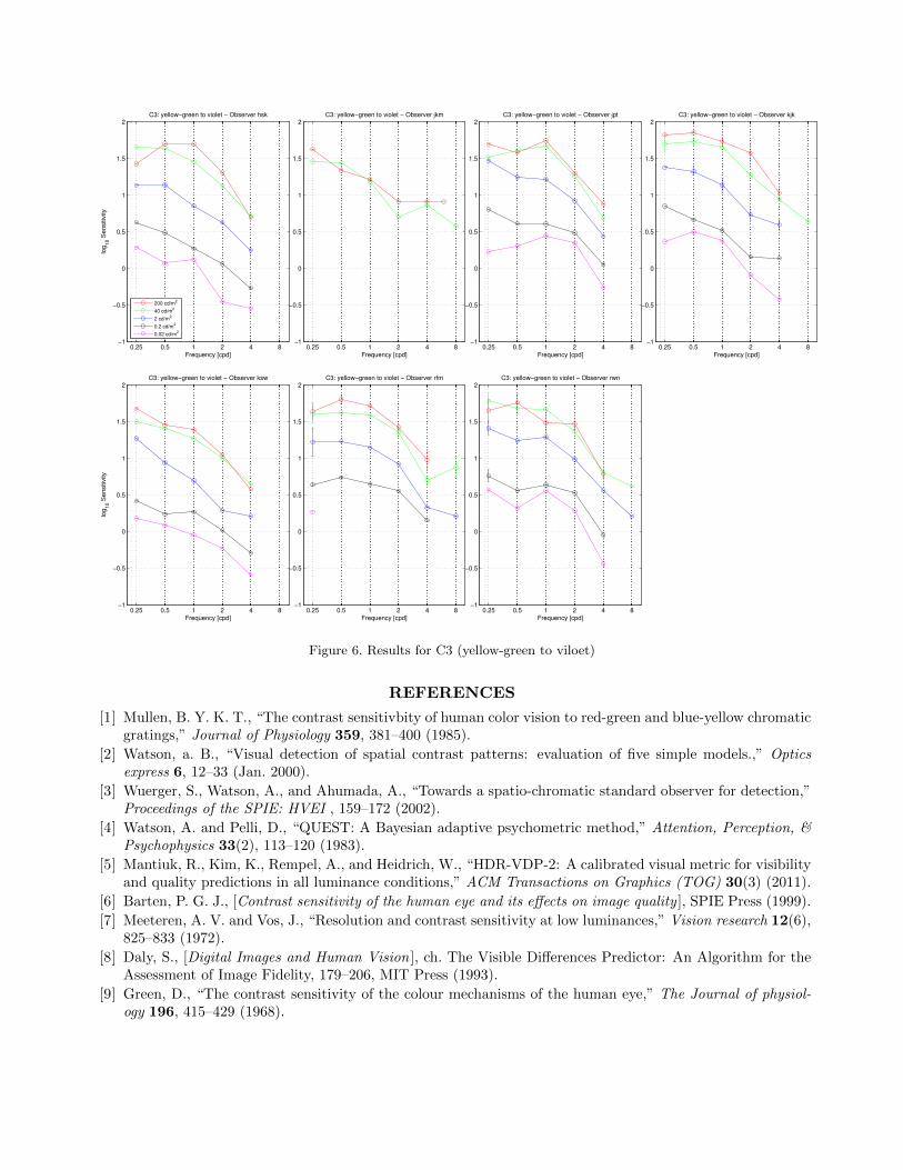
Figures 5 to 8 show the results of chromatic CSF measurements for individual observers and each color axisseparately. Overall, the measurements are relatively consistent across observers, but there are also significantdifferences. For some observers the CSF is low-pass (e.g. C2, 200 cd/m2, rfm and ksw), and for some it is band-pass (e.g. C2, 200 cd/m2, kjk and rwn). This is most likely due to the fact that we did not tune the color axesindividually for each observer to produce isoluminant stimuli for C2 and C3. Such isoluminant axes can be foundusing the flicker photometry method,11 in which the observers adjust the axis until the flicker at certain frequencyis the smallest. Moreover, the isoluminance is also changing with luminance level. As luminance decreases, therod vision starts to dominate detection. Since rod spectral sensitivity differ from cones, the isoluminance colorplanes also differs between photopic and scotopic luminance levels. Therefore, even though color axis C2 and C3were selected to produce isoluminant colors in terms of photopic vision and CIE standard observer, the stimulicontained a small amount of luminance contrast.

0.25 0.5 1 2 4 8 16

−0.5

0

0.5

1

1.5

2

2.5

3C2: green to red

Spatial frequency [cpd]

log

10 S

en

sitiv

ity

200 cd/m2

40 cd/m2

2 cd/m2

0.2 cd/m2

0.02 cd/m2

0.25 0.5 1 2 4 8 16

−0.5

0

0.5

1

1.5

2

2.5

3C3: yellow−green to violet

Spatial frequency [cpd]0.25 0.5 1 2 4 8 16

−0.5

0

0.5

1

1.5

2

2.5

3C6: dark−green to light−pink

Spatial frequency [cpd]0.25 0.5 1 2 4 8 16

−0.5

0

0.5

1

1.5

2

2.5

3C7: dark−yellow to light−blue

Spatial frequency [cpd]

Figure 4. Measurements for chromatic CSF (C2 and C3) and mixed chromatic and achromatic CSF (C6 and C7) —averaged over all observers.

4.4 Comparison with chromatic CSF models

Figure 9-left compares our results with ColorFest’s chromatic CSF models (model GSMa, fit for all observers).The data is plotted for the same luminance level as used in ColorFest measurements — 40 cd/m2. The ColorFestmodel predicts higher sensitivity loss for high frequencies than found in our measurements. Also, the sensitivityfor C2 was found to be lower in our measurements. The latter difference could be explained by different whitepoint of the background used in our experiemnts. When the white point from the ColorFest experiments is usedfor contrast calculation, the C3 sensitivity better matches the one predicted by the model.

The right-side of Figure 9 compares our results with the CSF used in the sCIELab — the spatial extension ofthe CIELab color difference metric.16 The functions were plotted after the Fourier transformation of the originalformula defined in the spatial domain [16, sec. 4] and using the parameters from the MATLAB implementationof the metric. These parameters differ from the ones reported in the paper because they are adjusted to ensurethat the CSF components sum to 1 (refer to the paper for details16). sCIELab CSF functions indicate strongerdrop of sensitivity for C2 and higher cut-off frequency for C3. However, it must be also noted that the color axisand luminance levels used in the sCIELab metric do not need to be the same as the ones used in our experiments.

The most likely explanation for the lower drop of sensitivity at high frequencies in our data is the intrusionof luminance signal in the stimuli. Unless the color axis is tuned separately for each individual observer andluminance level to ensure isoluminance, the stimuli will be partially detected by the achromatic mechanism.However, tuning color axis for individuals is certainly impractical for most visual models. Therefore, it could beargued that modelling chromatic mechanism with some amount of achromatic intrusion and thus lower drop athigh frequencies is likely to better predict the performance of an average observer.

5. CONCLUSION

To capture the effect of luminance on contrast detection of both chromatic and achromatic patterns, new CSFmeasurements were conducted for a range of luminance levels from 0.02 cd/m2 to 200 cd/m2. The goal was tocapture a possibly broad range of frequencies and luminance levels under the same viewing conditions. The focusof this study was on detection under natural viewing conditions, without restricting fixation point, controlling

0.25 0.5 1 2 4 80

0.5

1

1.5

2

2.5

3C2: green to red − Observer hsk

Frequency [cpd]

log

10 S

ensitiv

ity

200 cd/m2

40 cd/m2

2 cd/m2

0.2 cd/m2

0.02 cd/m2

0.25 0.5 1 2 4 80

0.5

1

1.5

2

2.5

3C2: green to red − Observer jkm

Frequency [cpd]0.25 0.5 1 2 4 8

0

0.5

1

1.5

2

2.5

3C2: green to red − Observer jpt

Frequency [cpd]0.25 0.5 1 2 4 8

0

0.5

1

1.5

2

2.5

3C2: green to red − Observer kjk

Frequency [cpd]

0.25 0.5 1 2 4 80

0.5

1

1.5

2

2.5

3C2: green to red − Observer ksw

Frequency [cpd]

log

10 S

ensitiv

ity

0.25 0.5 1 2 4 80

0.5

1

1.5

2

2.5

3C2: green to red − Observer rfm

Frequency [cpd]0.25 0.5 1 2 4 8

0

0.5

1

1.5

2

2.5

3C2: green to red − Observer rwn

Frequency [cpd]

Figure 5. Results for C2 (green to red)

pupil, or introducing temporal modulation. We believe that such conditions are more relevant if the data is tobe used for general visual models meant to predict performance for static images.

We found significant differences when our data was compared to popular CSF models of Barten and Daly. Weobserved higher sensitivity drop for higher frequencies and significant differences in sensitivities as compared tothese models in the luminance range between 0.02 and 2 cd/m2. We attribute these differences to the variationsin viewing conditions and stimuli.

Our measurements for chromatic CSF show a significant drop in sensitivity with luminance, but little changein the shape of the CSF. The drop of sensitivity at high frequencies is significantly weaker than reported in otherstudies and assumed in most chromatic CSF models.

In the future work, we wish to measure both chromatic and achromatic CSF at higher luminance levels.Such measurements will most probably involve a high-dynamic-range display. We also wish to measure thechromatic CSF for higher frequencies to clarify discrepancies between our measurements and popular chromaticCSF models. Finally, we plan to fit an analytical model that could be used to interpolate our data. Suchmodel was derived for our achromatic data,5 but a more general model that could explain both chromatic andachromatic data is needed.

ACKNOWLEDGMENTS

This work was partly supported by Mid-career Researcher Program through National Research Foundation ofKorea funded by the MEST (No. 2012-0005395).

0.25 0.5 1 2 4 8−1

−0.5

0

0.5

1

1.5

2C3: yellow−green to violet − Observer hsk

Frequency [cpd]

log

10 S

ensitiv

ity

200 cd/m2

40 cd/m2

2 cd/m2

0.2 cd/m2

0.02 cd/m2

0.25 0.5 1 2 4 8−1

−0.5

0

0.5

1

1.5

2C3: yellow−green to violet − Observer jkm

Frequency [cpd]0.25 0.5 1 2 4 8

−1

−0.5

0

0.5

1

1.5

2C3: yellow−green to violet − Observer jpt

Frequency [cpd]0.25 0.5 1 2 4 8

−1

−0.5

0

0.5

1

1.5

2C3: yellow−green to violet − Observer kjk

Frequency [cpd]

0.25 0.5 1 2 4 8−1

−0.5

0

0.5

1

1.5

2C3: yellow−green to violet − Observer ksw

Frequency [cpd]

log

10 S

ensitiv

ity

0.25 0.5 1 2 4 8−1

−0.5

0

0.5

1

1.5

2C3: yellow−green to violet − Observer rfm

Frequency [cpd]0.25 0.5 1 2 4 8

−1

−0.5

0

0.5

1

1.5

2C3: yellow−green to violet − Observer rwn

Frequency [cpd]

Figure 6. Results for C3 (yellow-green to viloet)

REFERENCES

[1] Mullen, B. Y. K. T., “The contrast sensitivbity of human color vision to red-green and blue-yellow chromaticgratings,” Journal of Physiology 359, 381–400 (1985).

[2] Watson, a. B., “Visual detection of spatial contrast patterns: evaluation of five simple models.,” Opticsexpress 6, 12–33 (Jan. 2000).

[3] Wuerger, S., Watson, A., and Ahumada, A., “Towards a spatio-chromatic standard observer for detection,”Proceedings of the SPIE: HVEI , 159–172 (2002).

[4] Watson, A. and Pelli, D., “QUEST: A Bayesian adaptive psychometric method,” Attention, Perception, &Psychophysics 33(2), 113–120 (1983).

[5] Mantiuk, R., Kim, K., Rempel, A., and Heidrich, W., “HDR-VDP-2: A calibrated visual metric for visibilityand quality predictions in all luminance conditions,” ACM Transactions on Graphics (TOG) 30(3) (2011).

[6] Barten, P. G. J., [Contrast sensitivity of the human eye and its effects on image quality ], SPIE Press (1999).

[7] Meeteren, A. V. and Vos, J., “Resolution and contrast sensitivity at low luminances,” Vision research 12(6),825–833 (1972).

[8] Daly, S., [Digital Images and Human Vision ], ch. The Visible Differences Predictor: An Algorithm for theAssessment of Image Fidelity, 179–206, MIT Press (1993).

[9] Green, D., “The contrast sensitivity of the colour mechanisms of the human eye,” The Journal of physiol-ogy 196, 415–429 (1968).

0.25 0.5 1 2 4 8 16−1

−0.5

0

0.5

1

1.5

2

2.5C6: dark−green to light−pink − Observer jkm

Frequency [cpd]

log

10 S

ensitiv

ity

40 cd/m2

2 cd/m2

0.25 0.5 1 2 4 8 16−1

−0.5

0

0.5

1

1.5

2

2.5C6: dark−green to light−pink − Observer kjk

Frequency [cpd]0.25 0.5 1 2 4 8 16

−1

−0.5

0

0.5

1

1.5

2

2.5C6: dark−green to light−pink − Observer pjj

Frequency [cpd]0.25 0.5 1 2 4 8 16

−1

−0.5

0

0.5

1

1.5

2

2.5C6: dark−green to light−pink − Observer rfm

Frequency [cpd]

0.25 0.5 1 2 4 8 16−1

−0.5

0

0.5

1

1.5

2

2.5C6: dark−green to light−pink − Observer rwn

Frequency [cpd]

log

10 S

ensitiv

ity

0.25 0.5 1 2 4 8 16−1

−0.5

0

0.5

1

1.5

2

2.5C6: dark−green to light−pink − Observer sks

Frequency [cpd]0.25 0.5 1 2 4 8 16

−1

−0.5

0

0.5

1

1.5

2

2.5C6: dark−green to light−pink − Observer syk

Frequency [cpd]

Figure 7. Results for C6 (dark-green to light-pink)

[10] Granger, E. M. and Heurtley, J. C., “Visual chromaticity-modulation transfer function,” Journal of theOptical Society of America 63, 1173 (Sept. 1973).

[11] Kelly, D. H., “Spatiotemporal variation of chromatic and achromatic contrast thresholds,” Journal of theOptical Society of America 73, 742 (June 1983).

[12] Hirai, K., Mikami, T., Tsumura, N., and Nakaguchi, T., “Measurement and Modeling of Chromatic Spatio-Velocity Contrast Sensitivity Function and its Application to Video Quality Evaluation,” in [Color ImagingConference ], 86–91 (2010).

[13] van der Horst, G. J. C. and Bouman, M. A., “Spatiotemporal Chromaticity Discrimination,” Journal of theOptical Society of America 59, 1482 (Nov. 1969).

[14] Rovamo, J. M., Kankaanpaa, M. I., and Kukkonen, H., “Modelling spatial contrast sensitivity functions forchromatic and luminance-modulated gratings,” Vision research 39(14), 2387–2398 (1999).

[15] Pattanaik, S. N., Ferwerda, J. A., Fairchild, M. D., and Greenberg, D. P., “A multiscale model of adaptationand spatial vision for realistic image display,” in [Proc. of SIGGRAPH’98 ], 287–298 (1998).

[16] Zhang, X. and Wandell, B. A., “A spatial extension of CIELAB for digital color-image reproduction,”Journal of the Society for Information Display 5(1), 61 (1997).

[17] Smith, V. C. and Pokorny, J., “Spectral sensitivity of the foveal cone photopigments between 400 and 500nm,” Vision Research 15(2), 161–171 (1975).

[18] Berns, R., “Methods for characterizing CRT displays,” Displays 16(4), 173–182 (1996).

0.25 0.5 1 2 4 8 16−1

−0.5

0

0.5

1

1.5

2

2.5C7: dark−yellow to light−blue − Observer jkm

Frequency [cpd]

log

10 S

ensitiv

ity

40 cd/m2

2 cd/m2

0.25 0.5 1 2 4 8 16−1

−0.5

0

0.5

1

1.5

2

2.5C7: dark−yellow to light−blue − Observer kjk

Frequency [cpd]0.25 0.5 1 2 4 8 16

−1

−0.5

0

0.5

1

1.5

2

2.5C7: dark−yellow to light−blue − Observer pjj

Frequency [cpd]0.25 0.5 1 2 4 8 16

−1

−0.5

0

0.5

1

1.5

2

2.5C7: dark−yellow to light−blue − Observer rfm

Frequency [cpd]

0.25 0.5 1 2 4 8 16−1

−0.5

0

0.5

1

1.5

2

2.5C7: dark−yellow to light−blue − Observer rwn

Frequency [cpd]

log

10 S

ensitiv

ity

0.25 0.5 1 2 4 8 16−1

−0.5

0

0.5

1

1.5

2

2.5C7: dark−yellow to light−blue − Observer sks

Frequency [cpd]0.25 0.5 1 2 4 8 16

−1

−0.5

0

0.5

1

1.5

2

2.5C7: dark−yellow to light−blue − Observer syk

Frequency [cpd]

Figure 8. Results for C7 (dark-yellow to light-blue)

[19] Macmillan, N., “Threshold estimation: The state of the art,” Attention, Perception, & Psychophysics 63(8),1277–1278 (2001).

[20] Watson, A. and Fitzhugh, A., “The method of constant stimuli is inefficient,” Attention, Perception, &Psychophysics 41(1), 87–91 (1990).

[21] Farell, B. and Pelli, D., “Psychophysical methods, or how to measure a threshold and why,” Vision research:A practical guide to laboratory methods 5, 129–136 (1999).

[22] Melcher, D. and Morrone, M., “Spatiotopic temporal integration of visual motion across saccadic eye move-ments,” Nature neuroscience 6, 877–881 (2003).

[23] Burr, D., Morrone, M., and Ross, J., “Selective suppression of the magnocellular visual pathway duringsaccadic eye movements,” Nature 371, 511–513 (1994).

[24] Solomon, J. and Pelli, D., “The visual filter mediating letter identification,” Nature 369, 395–397 (1994).

[25] Brainard, D., “The psychophysics toolbox,” Spatial vision 10, 433–436 (1997).

[26] Peli, E., Yang, J. a., Goldstein, R., and Reeves, a., “Effect of luminance on suprathreshold contrast percep-tion.,” Journal of the Optical Society of America. A, Optics and image science 8, 1352–9 (Aug. 1991).

[27] van Nes, F. L. and Bouman, M. A., “Spatial Modulation Transfer in the Human Eye,” Journal of the OpticalSociety of America 57, 401 (Mar. 1967).

[28] Stromeyer, C. F. and Julesz, B., “Spatial-Frequency Masking in Vision: Critical Bands and Spread ofMasking,” Journal of the Optical Society of America 62, 1221 (Oct. 1972).

0.125 0.25 0.5 1 2 4 8 160

0.5

1

1.5

2

2.5

3

3.5Compared with ColorFest CSF

Spatial frequency [cpd]

log

10 S

ensitiv

ity

C2: red to green

C3: yellow−green to violet

0.125 0.25 0.5 1 2 4 8 160

0.5

1

1.5

2

2.5

3

3.5Compared with sCIELAB CSF

Spatial frequency [cpd]

log

10 S

ensitiv

ity

C2: red to green

C3: yellow−green to violet

Figure 9. Comparison of our measurements of the chromatic CSFs at 40 cd/m2 background luminance with ColorFestCSF model (left) and with the CSF used in the sCIELab metric (right). Our measurements are plotted as dashed lineswith error bars while the models are plotted with solid lines.

[29] Savoy, R. L. and Mccann, J. J., “Visibility of low-spatial-frequency sine-wave targets: Dependence onnumber of cycles,” Journal of the Optical Society of America 65(3) (1975).