measurement science for engineers || measurement errors and uncertainty
TRANSCRIPT
Chapter 3
Measurement Errors and Uncertainty
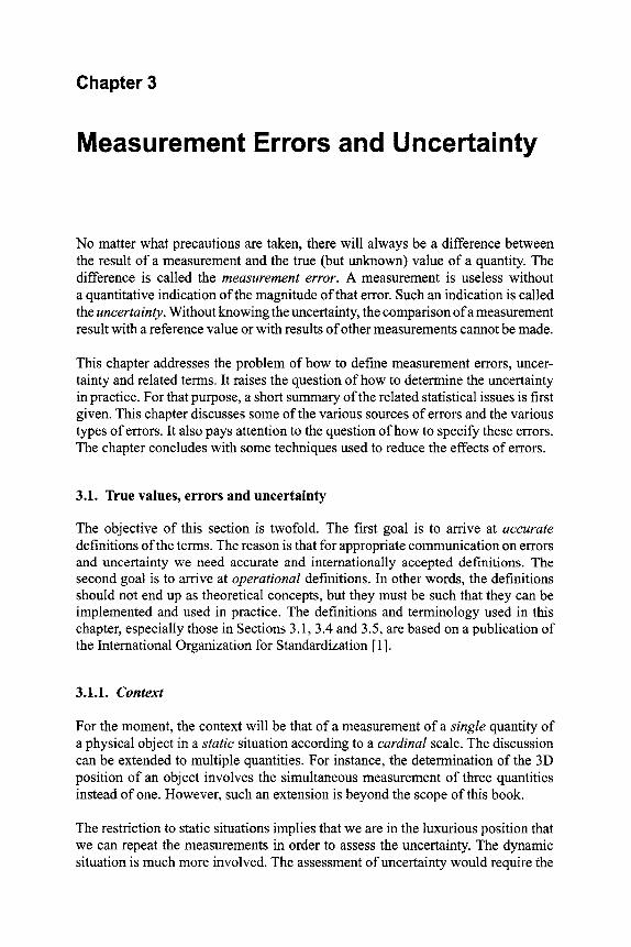
No matter what precautions are taken, there will always be a difference between the result of a measurement and the true (but unknown) value of a quantity. The difference is called the measurement error. A measurement is useless without a quantitative indication of the magnitude of that error. Such an indication is called the uncertainty. Without knowing the uncertainty, the comparison of a measurement result with a reference value or with results of other measurements cannot be made.
This chapter addresses the problem of how to define measurement errors, uncer- tainty and related terms. It raises the question of how to determine the uncertainty in practice. For that purpose, a short summary of the related statistical issues is first given. This chapter discusses some of the various sources of errors and the various types of errors. It also pays attention to the question of how to specify these errors. The chapter concludes with some techniques used to reduce the effects of errors.
3.1. True values, errors and uncertainty
The objective of this section is twofold. The first goal is to arrive at accurate definitions of the terms. The reason is that for appropriate communication on errors and uncertainty we need accurate and internationally accepted definitions. The second goal is to arrive at operational definitions. In other words, the definitions should not end up as theoretical concepts, but they must be such that they can be implemented and used in practice. The definitions and terminology used in this chapter, especially those in Sections 3.1, 3.4 and 3.5, are based on a publication of the International Organization for Standardization [ 1 ].
3.1.1. Context
For the moment, the context will be that of a measurement of a single quantity of a physical object in a static situation according to a cardinal scale. The discussion can be extended to multiple quantities. For instance, the determination of the 3D position of an object involves the simultaneous measurement of three quantities instead of one. However, such an extension is beyond the scope of this book.
The restriction to static situations implies that we are in the luxurious position that we can repeat the measurements in order to assess the uncertainty. The dynamic situation is much more involved. The assessment of uncertainty would require the

44 Measurement Science for Engineers
availability of models describing the dynamic behaviour of the process. This too is beyond the scope of the chapter.
Different scales require different error analyses. For instance, the uncertainty of a burglar alarm (nominal scale) is expressed in terms of"false alarm rate" and"missed event rate". However, in this chapter, measurements other than with a cardinal scale are not considered.
3.1.2. Basic definitions
The particular quantity to be measured is called a measurand. Its (true) value, x, is the result that would be obtained by a perfect measurement. Since perfect meas- urements are only imaginary, a true value is always indeterminate and unknown. The value obtained by the measurement is called the result o f the measurement and is denoted here by the symbol z. The (measurement) error, e, is the difference between measurement result and the true value:
e = z - x (3.1)
Because the notion of error is defined in terms of the unknown"true value", the error is unknown too. Nevertheless, when evaluating a measurement, the availability of the error can be so urgent that in the definition of "measurement error" the phrase "true value" is sometimes replaced by the so-called conventional true value. This is a value attributed to the quantity, and that is accepted as having an uncertainty small enough for the given purpose. Such a value could, for instance, be obtained from a reference standard.
The relative error ere! is the error divided by the true value, i.e. erel = e/x . In order to distinguish the relative error from the ordinary error, the latter is sometimes called absolute error. The term is ambiguous since it can also mean lel, but in this book the former denotation will be used.
The term accuracy of a measurement refers to a qualification of the expected closeness of the result of a measurement and the true value. The generally accepted, quantitative measure related to accuracy is uncertainty. The uncertainty of a meas- urement is a parameter that characterizes the range of the values within which the true value of a measurement lies. It expresses the lack of knowledge that we have on the measurand. Before proceeding to a precise definition of uncertainty some concepts from probability theory must be introduced.
3.2. Measurement error and probability theory
The most common definition of uncertainty is based on a probabilistic model in which the actual value of the measurement error is regarded as the outcome of a so-called "stochastic experiment". The mathematical definition of a stochastic experiment is complicated and as such not within the scope of this book. See [2]
Measurement Errors and Uncertainty 45
for a comprehensive treatment of this subject. However, a simple view is to regard a stochastic experiment as a mathematical concept that models the generation of random numbers. The generation of a single random number is called a trial. The particular value of that number is called the outcome or realization of that trial. After each trial, a so-called random variable takes the outcome as its new value. Random variables are often denoted by an underscore. Hence, z is the notation for the result of a measurement, and e is the notation of the measurement error, both regarded as random variables. Each time that we repeat our measurement, z and e take different values.
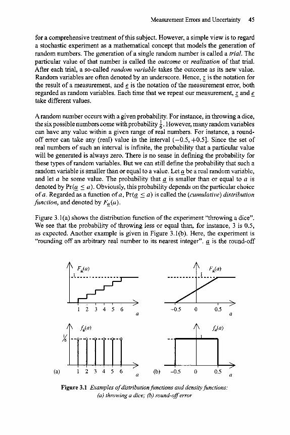
A random number occurs with a given probability. For instance, in throwing a dice, the six possible numbers come with probability 1. However, many random variables can have any value within a given range of real numbers. For instance, a round- off error can take any (real) value in the interval ( -0 .5 , +0.5]. Since the set of real numbers of such an interval is infinite, the probability that a particular value will be generated is always zero. There is no sense in defining the probability for these types of random variables. But we can still define the probability that such a random variable is smaller than or equal to a value. Let a be a real random variable, and let a be some value. The probability that a is smaller than or equal to a is denoted by Pr(a < a). Obviously, this probability depends on the particular choice ofa. Regarded as a function of a, Pr(a < a) is called the (cumulative) distribution function, and denoted by Fa (a).
Figure 3.1 (a) shows the distribution function of the experiment "throwing a dice". We see that the probability of throwing less or equal than, for instance, 3 is 0.5, as expected. Another example is given in Figure 3.1(b). Here, the experiment is "rounding off an arbitrary real number to its nearest integer", a is the round-off
(a)
Fa(a) 1
I 1 !
I I
I i i i
1 2 3 4 5 6
_ )
J
-0.5 0 0.5 a a
fa(a)
I I I I I I
1 2 3 4 5 6 J
|
~(a)
J
(b) -0.5 0 0.5 a a
Figure 3.1 Examples of distribution functions and density functions: (a) throwing a dice; (b) round-off error

46 Measurement Science for Engineers
error. (These types of errors occur in AD-conversion; see Chapter 6.) Obviously, the main difference between the distribution functions of Figures 3.1 (a) and (b) is that the former is discrete (stepwise) and the latter is continuous. This reflects the fact that the number of possible outcomes in throwing a dice is finite, whereas the number of outcomes of a round-off error is infinite (i.e. any real number within ( -0 .5 , +0.5]).
Figure 3.1 illustrates the fact that Fa(a) is a non-decreasing function with Fa(-Oo) = 0, and Fa(c~) = 1. Simply stated, Fa(-C~) = 0 means that a is never smaller than - c~ . Fa (oo) = 1 means that a is always smaller than +c~.
The distribution function facilitates the calculation of the probability that a random variable takes values within a given range:
Pr(al < a < a 2 ) = F a ( a 2 ) - F a ( a l ) (3 .2 )
If Fa (a) is continuous, then, in the limiting case as al approaches a2, equation (3.2) turns into"
dFa(a) lim Pr(al < a < a 2 ) - - ( a 2 - a l ) da
a l ----> a2 a--a l
(3.3)
The first derivative of Fa(a) is called the (probability) density function 1 fa(a)"
dFa(a) fa(a) = - (3.4)
- da
Figure 3.1 (b) shows the density function for the "round-offerror" cases. The density function shows that the error is uniformly distributed in the interval ( -0 .5, +0.5]. Hence, each error within that interval is evenly likely.
The first derivative of a step function is called a Dirac-function 3(.). With that, even if the random variable is discrete, the definition of the density function holds. Each step-like transition in the distribution function is seen as a Dirac function in the density function, the weight of which equals the step height. Figure 3.1(a) shows the density function belonging to the "dice" experiment. This density is
1 For brevity, the shorter notation f(a) is used instead of fa(a), but this is only allowed m
in a context without any chance of confusion with other random variables. Sometimes, one uses p(a) instead of f(a), for instance, if the symbol f(.) has already been used for another purpose.

Measurement Errors and Uncertainty 47
0.5
0.4
0.3
0.2
0.1
0 ---.z
normal distribution
fa(a) # = 0 o'=1
-2 0 2 a 4
0.25
0.2
0.15
0.1
0.05
ol 0
Poisson distribution
fa(a)
2=5
TT•a.. 10 a 15
uniform distribution
"~fa(a) (~ -A) -1
---~a B
binomial distribution 0.25
fa(a),
0.2
0.15
0.1
0.05
0 0
N=15 P=0.25
5 15 l lTa . . . . .
10 a
Figure 3.2 Density functions
expressed as Z6=l ~8(a - n). The figure shows the six Dirac functions with 1 weights $.
3.2.1. Some important density functions
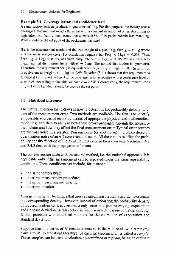
Some density functions frequently met in measurement systems are (see Figure 3.2):
The normal distribution with parameters/z and a"
f a ( a ) = 1 ( (a -/x)2 ) (3.5) - a ~ e x p - 2o.2
The uniform distribution with parameters A and B"
1
f a ( a ) = B - A 0
i f A < a < B
elsewhere (3.6)

48 Measurement Science for Engineers
The Poisson distribution with parameter ~.:
oo ~.n exp(-~.)
fa (a) = ~ n! n=0
8(a - n ) (3.7)
The binomial distribution with parameter N and P
oo N!
fa(a) = ~ n!(N- n)l II~-0
pn(1 - P ) N - n s ( a - n) (3.8)
Normal distributions (also called Gaussian distributions) occur frequently, both in physical models and in mathematical analysis. Any physical quantity that is an additive accumulation of many independent random phenomena is normally distributed. An example is the noisy current of a resistor. Such a current is induced by the thermal energy that causes random movements of the individual electrons. Altogether, these individual movements give rise to a random current that obeys a normal distribution. An advantage of the normal distribution is that some of its properties (to be discussed later) facilitate mathematical analysis whereas in the case of other distributions such an analysis is difficult.
As said before, the uniform distribution is used in AD-conversion and other round- off processes in order to model quantization.
The Poisson distribution and the binomial distribution are both discrete. The Poisson distribution models the process of counting events during a period of time. An example is a photo detector. The output of such a device is proportional to the number of photons that are intercepted on a surface during a period of time (sim- ilar to how rain intensity is measured by accumulating raindrops in a rain gauge). The parameter ~. is the mean number of counts.
The binomial distribution occurs whenever the experiment consists of N independ- ent trials of a Boolean random variable. P is the probability that such a variable takes the value "true", and hence, 1 - P is the probability of "false". The ran- dom number returned by the binomial experiment is the number of times that the Boolean variable gets the value "true".
Since both the Poisson distribution and the binomial distribution find their origin in a counting process of individual events (and thus phenomena that are caused by a number of independent random sources) we might expect that these distributions both approximate the normal distribution. This is indeed the case. The Poisson dis- tribution can be approximated by a normal distribution with/x = ~ and a = ~/~. if,~ is large enough. The binomial distribution corresponds to a normal distribution with # = NP and tr = ~/[NP(1 - P)] provided that N is sufficiently large. However, we have to take into account that both the Poisson and the binomial distribution are discrete, whereas the normal distribution is continuous. In fact, it is the envelope of the discrete distributions that is well approximated by the normal distribution.
Measurement Errors and Uncertainty 49
3.2.2. Expectation, variance and standard deviation
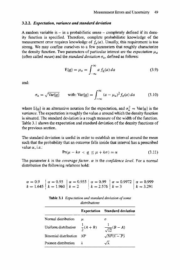
A random variable i s - in a probabilistic sense- completely defined if its dens- ity function is specified. Therefore, complete probabilistic knowledge of the measurement error requires knowledge of fa (a). Usually, this requirement is too strong. We may confine ourselves to a few parameters that roughly characterize the density function. Two parameters of particular interest are the expectation tZa (often called mean) and the standard deviation era, defined as follows:
E{a} = l % a - - a fa(a) da O0
(3.9)
and:
F era = v/Var{a} with: Var{a} -- (a - lZa)2 fa (a) da (3.10) (X)
where E{a} is an alternative notation for the expectation, and aa 2 = Var{a} is the variance. The expectation is roughly the value a around which the density function is situated. The standard deviation is a rough measure of the width of the function. Table 3.1 shows the expectation and standard deviation of the density functions of the previous section.
The standard deviation is useful in order to establish an interval around the mean such that the probability that an outcome falls inside that interval has a prescribed value ~, i.e.:
Pr(/x - ka < a </% + ka) = c~ (3.11)
The parameter k is the coverage factor, ot is the confidence level. For a normal distribution the following relations hold:
a = 0 . 9 c~=0.95 a = 0 . 9 5 5 a = 0 . 9 9 a = 0 . 9 9 7 2 a = 0 . 9 9 9 k = 1 . 6 4 5 k = 1 . 9 6 0 k = 2 k = 2 . 5 7 6 k = 3 k = 3 . 2 9 1
Table 3.1 Expectation and standard deviation of some distributions
Expectation Standard deviation
Normal distribution /%
1 Uniform distribution ~ (A + B)
Binomial distribution NP
Poisson distribution ~.
(7
1 A)
,/NP ( ~ - P)
50 Measurement Science for Engineers
Example 3.1 Coverage factor and confidence level A sugar factory sells its products in quantities of 1 kg. For that purpose, the factory uses a packaging machine that weighs the sugar with a standard deviation of 5 mg. According to legislation, the factory must assure that at most 0.5% of its packs contain less than 1 kg. What should be the set point of the packaging machine?
If z is the measurement result, and the true weight of a pack is x, then x = z - e where e is the measurement error. The legislation requires that Pr(_x_ < 1 kg) = 0.005. Thus, Pr(z - e < 1 kg) = 0.005, or equivalently Pr(e > z - 1 kg) = 0.005. We assume a zero mean, normal distribution for e with cr = 5 mg. The normal distribution is symmetric. Therefore, the requirement for z is equivalent to: Pr(lel > z - 1 kg) = 0.01. In turn, this is equivalent to Pr(lel < z - 1 kg) = 0.99. Equation (3.11) shows that this requirement is fulfilled if kcr = z - 1, where k is the coverage factor associated with a confidence level of ct = 0.99. According to the table we have k = 2.576. Consequently, the requirement leads to z = 1.0129 kg which should be used as the set point.
3.3. Statistical inference
The natural question that follows is how to determine the probability density func- tion of the measurement error. Two methods are available. The first is to identify all possible sources of errors by means of appropriate physical and mathematical modelling, and then to analyze how these errors propagate through the measure- ment chain and how they affect the final measurement error. Typical error sources are thermal noise in a resistor, Poisson noise (or shot noise) in a photo detector, quantization noise of an AD converter, and so on. All these sources affect the prob- ability density function of the measurement error in their own way. Sections 3.4.2 and 3.4.3 deal with the propagation of errors.
The current section deals with the second method, i.e. the statistical approach. It is applicable only if the measurement can be repeated under the same repeatability conditions. These conditions can include, for instance:
�9 the same temperature; �9 the same measurement procedure; �9 the same measuring instrument; �9 the same location.
Histogramming is a technique that uses repeated measurements in order to estimate the corresponding density. However, instead of estimating the probability density of the error, it often suffices to estimate only some of its parameters, e.g. expectat ion and standard deviation. In this section is first discussed the issue ofhis togramming. It then proceeds with statistical methods for the estimation of expectation and standard deviation.
Suppose that in a series of N measurements Zn is the n-th result with n ranging from 1 to N. In statistical literature [3] each measurement Zn is called a sample. These samples can be used to calculate a normalized histogram, being an estimate

Measurement Errors and Uncertainty 51
of the probability density of z. Often, we are interested in the probability density of e, not in z. If this is the case, we need to have a "conventional true value" x (see Section 3.1.2) so that we are able to calculate the error associated with each measurement: en = Zn - x ; see equation (3.1). These errors can be used to estimate the probability density of e.
3.3.1. Estimation o f density functions: histograms
Lets assume that we want to estimate the probability density of a real random variable a. Here, a stands for the measurement result z, or for the measurement
m ~ u
error e, or for whatever is applicable. We have a set of N samples an that are all realizations of the random variable a. Furthermore, we assume that these samples are statistically independent. Let amin and amax be the minimum and maximum value of the series an. We divide the interval [amin, amax] into K equally sized sub- intervals (ak, ak + Aa] where Aa = (amax -amin ) /K . Such a sub-interval is called a bin. We count the number of outcomes that fall within the k-th bin, and assign that count to the variable hk. The probability that a sample falls in the k-th bin is:
f ak+Aa
Pt~ = fa(a)da ,J ak
(3.12)
Since we have N samples, hk has a binomial distribution with parameters (N, Pk) (see Section 3.2.1). Thus, the expectation of hk is E{hk} = NPk and its variance is NPk(1 - Pk); see Table 3.1.
The normalized histogram is:
The expectation of Hk is:
hk Hk = (3.13)
N A a
E{hk} Pk E{Hk} -- --
N A a Aa
I f ak+Aa ( 1 ) fa (a)da ,~ fa ak + -~ Aa (3.14)
Aa a ak -- --
Therefore, Hk is an estimate for fa(ak + 1 Aa).
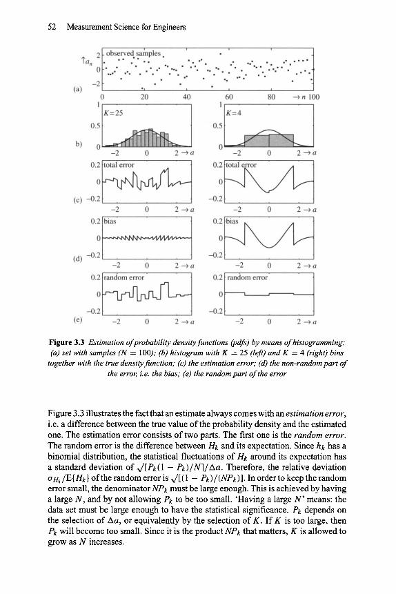
Figure 3.3(a) shows 100 outcomes of a normally distributed, random variable. Two (normalized) histograms have been derived from that data set and plotted in the figure together with the true probability density. In the real world, the true density is always unknown. Here, we have used data whose density function is known, so that we can evaluate the accuracy of the estimated density. One histogram is calculated with K = 4, the other with K = 25. The normalized histogram provides estimates for fa( ') only at a finite number of values of a, i.e. at ak + 1 Aa. At all other values of a we need to interpolate. In Figure 3.3 this is done by so-called zero order interpolation (also called nearest neighbour interpolation)" i fa falls in the k-th bin, then fa(a) is estimated by Hk. This kind of interpolation gives rise to the blockish appearance of the histograms, as shown in the figure.
52 Measurement Science for Engineers
Figure 3.3 Estimation of probability density functions (pdfs) by means of histogramming: (a) set with samples (N = 100); (b) histogram with K = 25 (left) and K = 4 (right) bins
together with the true density function; (c) the estimation error; (d) the non-random part of the error, i.e. the bias; (e) the random part of the error
Figure 3.3 illustrates the fact that an estimate always comes with an estimation error, i.e. a difference between the true value of the probability density and the estimated one. The estimation error consists of two parts. The first one is the random error. The random error is the difference between Hk and its expectation. Since hk has a binomial distribution, the statistical fluctuations of Hk around its expectation has a standard deviation of ~/[Pk(1 - P k ) / N ] / A a . Therefore, the relative deviation tri-ik/E { Hk } of the random error is ~/[ ( 1 - Pk ) / (NPk) ]. In order to keep the random error small, the denominator NPk must be large enough. This is achieved by having a large N, and by not allowing Pk to be too small. 'Having a large N ' means: the data set must be large enough to have the statistical significance. Pk depends on the selection of Aa, or equivalently by the selection of K. If K is too large, then Pk will become too small. Since it is the product NPk that matters, K is allowed to grow as N increases.

Measurement Errors and Uncertainty 53
The second type of error is the bias. The bias is the estimation error that persists with a fixed value of K, even if N becomes infinitely large, and thus even if the random error is negligible. In other words, the bias is an error that is inherent to the estimation method, and that is not caused by the randomness of the data set.
The first reason for the bias is the approximation that is used in equation (3.14). The approximation is only accurate if Aa is small. In other words, K must be large to have a close approximation. If Aa is not sufficiently small, then the approxim- ation causes a large bias. The second reason for the bias is the interpolation. The nearest neighbour interpolation gives rise to an interpolation error. Especially, the interpolation can become large for values of a that are far away from a bin centre. Therefore, here too, K must be large to have a small error.
Figure 3.3 illustrates the influence of K on the two types of errors. If K is small, and the bins are wide, the random error is relatively small, but then the bias is large. If K is large, and the bins are narrow, the random error is large, and the bias is small. A trade-off is necessary. A reasonable rule of thumb is to choose K = ~/N.
Example 3.2 Bias and random errors in density estimation The table below shows the maximum values of the various errors for the example of Figure 3.3. The maximum is calculated over all values of a. The maximum errors which occur when K = ~/N = 10 is selected are also shown:
K = 2 5 K = 1 0 K = 4
Max total error 0.16 0.12 0.19 Max bias 0.03 0.07 0.18 Max random error 0.14 0.05 0.02
Clearly, when K = 25, the random error prevails. But when K = 4, the bias prevails. However, when K = 10, the bias and random error are about of the same size. Such a balance between the two error types minimizes the total error.
3.3.2. E s t i m a t i o n o f m e a n a n d s t a n d a r d d e v i a t i o n
The obvious way to estimate the mean of the error a from a set of samples an is to use the average fi of the set 2"
1 N fZa --" ~l - - an
n=l (3.15)
2 The notation ~ is often used to indicate the result of an averaging operator applied to a set an.

54 Measurement Science for Engineers
The symbol "^" on top of a parameter is always used to indicate that it is an estimate of that parameter. Thus/~a is an estimate of #a.
The set an can be associated with a set of random variables a n (all with the same distribution as a) . Therefore, the average (being a weighted sum of an) can also be associated with a random variable" /2 a. Consequently, the average itself has a mean, variance and standard deviation:
E{/2a} = / Z a (3 .16)
1 Var{/2a} = --Var{an} (3.17)
- - N
1 0"/~ a "-- ~f--.~ O" a (3.18)
V/V
The proof can be found in Appendix C. Equation (3.17) is valid under the condition that the cross products E{ (a n - - / Z a ) ( a m - - / Z a ) } vanish for all n # m. If this is the case, then the set an is said to be uncorrelated.
The bias, being the non-random part of the estimation error, is the difference between the true parameter and the mean of the estimate. Equation (3.16) shows that the bias of the average is zero. Therefore, the average is said to be an unbiased estimator. The standard deviation of the estimator is proportional to 1/~/N. In the limiting case, as N ~ oo, the estimation error vanishes. An estimator with such a property is said to be consistent.
The unbiased estimation of the variance Var{a} is more involved. We have to distinguish two cases. The first case is when the mean/Za is fully known. An efficient estimator is:
~ 1 N N E (an --/Za) 2 = (a - lZa) 2
n=l (3.19)
In the second case, both the mean and the variance are unknown, so that they must be estimated simultaneously. The mean is estimated by the average/2a - fi as before. Then, the variance can be estimated without bias by the so-called sample variance S 2:
N Sa2= N -1 _ _ N-----~N (a ~)---------~ (3.20) 1 E (an --t~) 2 - " - -
n = l
Apparently, we need a factor N/(N - 1) to correct the bias in (a - ~ ) 2 . Without this correction factor, Sa 2 would be too optimistic, i.e. too small. The background
of this is that, in the uncorrected estimate, i.e. in (a - fi)2, the term ~ absorbs a part of the variability of the set an. In fact, ~ is the value of the parameter a that
minimizes the expression (a - ct) 2. For instance, in the extreme case N = 1, we
have fi = al and (a - h)2 = 0. The latter would be a super-optimistic estimate for
Measurement Errors and Uncertainty 55
the variance. However, if N = 1, then S 2 is indeterminate. This exactly represents our state of knowledge about the variance if we have only one sample.
As said before, these estimators are unbiased. The estimation error that remains is quantified by their variances (see Appendix C):
Var{62} = 2an4 Var{Sa 2} = 2an4 (3.21) N N - 1
Strictly speaking, these last expressions are valid only if an is normally distributed.
Equations (3.18) and (3.21) impose the problem that in order to calculate O ' / ~ a ,
Var{& 2} or Var{S 2} we have to know aa. Usually, this problem is solved by substituting &a or Sa for aa.
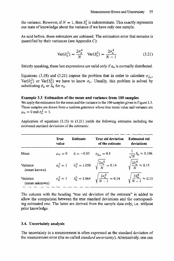
Example 3.3 Est imation of the mean and variance from 100 samples We apply the estimators for the mean and the variance to the 100 samples given in Figure 3.3. These samples are drawn from a random generator whose true mean value and variance are /~a = 0 ando-a 2 = 1.
Application of equations (3.15) to (3.21) yields the following estimates including the estimated standard deviations of the estimates:
True Estimate True std deviation Estimated std value of the estimate deviations
1 Mean /Za - - - 0 a "-- - - 0 . 0 5 o-~a = 0.1 Vr_~Sa ~ 0.106
Variance o '2=1 62=1.056 ~2o'4 = 0.14 ~2N4 ~ 0.15 (mean known) N
Variance o'2--1 $2=1.064 ~/ 2o-4 --0.14 V / 2S4 - ,~ 0.15 (mean unknown) N - 1 N - 1
The column with the heading "true std deviation of the estimate" is added to allow the comparison between the true standard deviations and the correspond- ing estimated one. The latter are derived from the sample data only, i.e. without prior knowledge.
3.4. Uncertainty analysis
The uncertainty in a measurement is often expressed as the standard deviation of the measurement error (the so-called standard uncertainty). Alternatively, one can
56 Measurement Science for Engineers
use the term expanded uncertainty which defines an interval around the meas- urement result. This interval is expected to encompass a given fraction of the probability density associated with the measurement error; see equation (3.11). Assuming a normal distribution of the measurement error, the standard uncertainty can be transformed to an expanded uncertainty by multiplication of a coverage factor.
In practice, there are two methods to determine the standard uncertainty. The first method is the statistical approach, based on repeated measurements (sometimes called type A evaluation o f uncertainty). The second approach is based on a priori distributions (the type B evaluation).
3.4.1. Type A evaluat ion
The goal of type A evaluation is to assess the components that make up the uncertainty of a measurement. It uses statistical inference techniques applied to data acquired from the measurement system. Examples of these techniques are histogramming (Section 3.3.1), and estimation of mean and standard deviation (Section 3.3.2). Many other techniques exist, such as curve fitting and analysis of variance, but these techniques are not within the scope of this book. Type A evaluation is applicable whenever a series of repeated observations of the system are available. The results of type A evaluation should be taken with care because statistical methods easily overlook systematic errors (see Section 3.5.1).
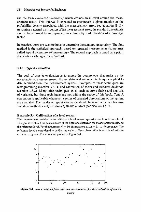
E x a m p l e 3.4 Cal ibrat ion of a level sensor The measurement problem is to calibrate a level sensor against a stable reference level. The goal is to obtain the best estimate of the difference between the measurement result and the reference level. For that purpose N = 50 observations Zn, n = 1 . . . . . N are made. The reference level is considered to be the true value x. Each observation is associated with an error en = Zn - x. The errors are plotted in Figure 3.4.
4
e n
2
-2
I I I I
# w �9 #
# # �9 # # Im �9
Im �9 �9 �9 # #w
�9 wm �9
8
�9 �9 B m
B B
- - 4 i i i i
l 10 20 30 40
Figure 3.4 Errors obtained from repeated measurements for the calibration o f a level
sensor
Measurement Errors and Uncertainty 57
If we assume that the observations are independent, the best estimate for the difference is the average of en. Application of equation (3.15) yields: ~ = 0.58 mm. The estimated standard deviation of the set en follows from equation (3.20): Se = 1.14 mm. According to equation (3.18) the standard deviation of the mean is ~ = ~e/,v/-N ~ Se/VCN = 0.16mm.
The conclusion is that, at the reference level, the sensor should be corrected by a term ~, = 0.58 mm. However, this correction introduces an uncertainty of 0.16 mm.
3.4.2. Type B evaluation
The determination of the uncertainty based on techniques other than statistical inference is called type B evaluation. Here, the tmcertainty is evaluated by means of a pool of information that is available on the variability of the measurement result:
�9 The specifications of a device as reported by the manufacturer. �9 Information obtained from a certification procedure, for instance, on behalf of
calibration. �9 Information obtained from reference handbooks. �9 General knowledge about the conditional environment and the related physical
processes.
The principles will be clarified by means of an example:
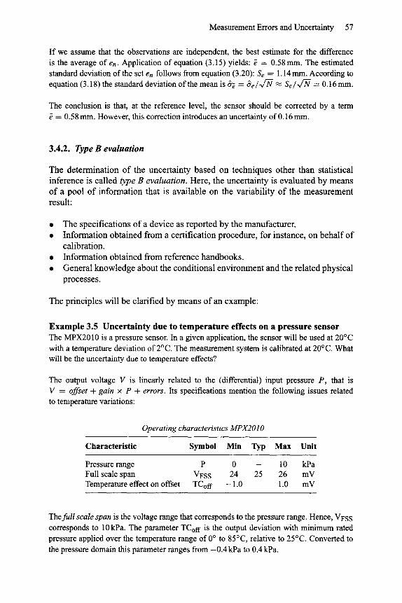
Example 3.5 Uncertainty due to temperature effects on a pressure sensor The MPX2010 is a pressure sensor. In a given application, the sensor will be used at 20~ with a temperature deviation of 2~ The measurement system is calibrated at 20~ What will be the uncertainty due to temperature effects?
The output voltage V is linearly related to the (differential) input pressure P, that is V = offset + gain x P + errors. Its specifications mention the following issues related to temperature variations:
Operating characteristics MPX2010
Characteristic Symbol Min Typ Max Unit
Pressure range P 0 - 10 kPa Full scale span VFS S 24 25 26 mV Temperature effect on offset TCoff -1 .0 - 1.0 mV
The full scale span is the voltage range that corresponds to the pressure range. Hence, VFSS corresponds to 10 kPa. The parameter TCoff is the output deviation with minimum rated pressure applied over the temperature range of 0 ~ to 85~ relative to 25~ Converted to the pressure domain this parameter ranges from -0.4 kPa to 0.4 kPa.
58 Measurement Science for Engineers
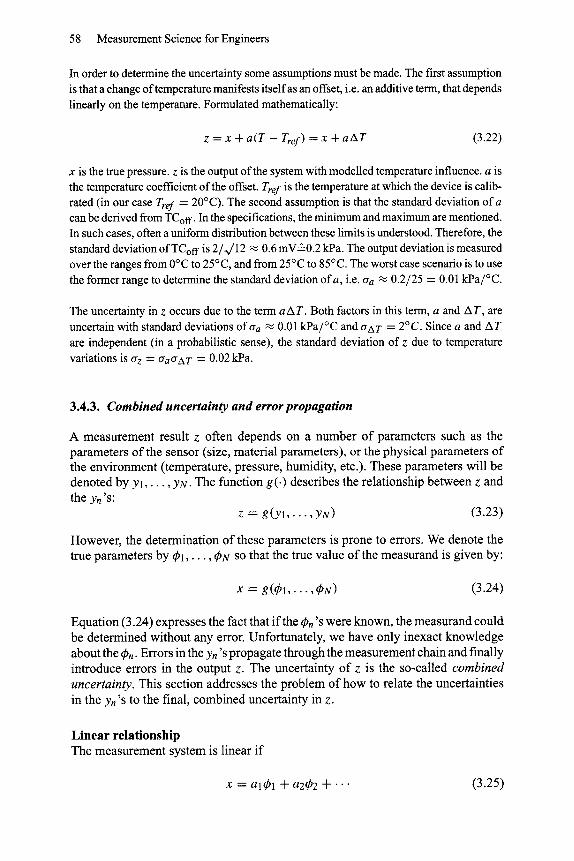
In order to determine the uncertainty some assumptions must be made. The first assumption is that a change of temperature manifests itself as an offset, i.e. an additive term, that depends linearly on the temperature. Formulated mathematically:
z = x + a ( T - Tref) = x + a A T (3.22)
x is the true pressure, z is the output of the system with modelled temperature influence, a is the temperature coefficient of the offset. Tref is the temperature at which the device is calib- rated (in our case Tref = 20~ The second assumption is that the standard deviation of a can be derived from TCof f. In the specifications, the minimum and maximum are mentioned. In such cases, often a uniform distribution between these limits is understood. Therefore, the standard deviation of TCoff is 2/~/12 .~ 0.6 mV~0.2 kPa. The output deviation is measured over the ranges from 0~ to 25~ and from 25~ to 85~ The worst case scenario is to use the former range to determine the standard deviation of a, i.e. ~ra ~ 0.2/25 = 0.01 kPa/~
The uncertainty in z occurs due to the term a A T. Both factors in this term, a and A T, are uncertain with standard deviations ofcra ~ 0.01 kPa/~ and crAT = 2~ Since a and AT are independent (in a probabilistic sense), the standard deviation of z due to temperature
variations is ~r z - CracrAT -- 0.02 kPa.
3.4.3. Combined uncertainty and error propagation
A measurement result z often depends on a number of parameters such as the parameters of the sensor (size, material parameters), or the physical parameters of the environment (temperature, pressure, humidity, etc.). These parameters will be denoted by Yl,. �9 YN. The function g(.) describes the relationship between z and the yn'S:
z -- g ( Y l , . . . , YN) (3.23)
However, the determination of these parameters is prone to errors. We denote the true parameters by ~1,. �9 ~N so that the true value of the measurand is given by:
X -- g ( t ~ l , . . . , ~N) (3.24)
Equation (3.24) expresses the fact that if the ~n 'S were known, the measurand could be determined without any error. Unfortunately, we have only inexact knowledge about the q~n. Errors in the yn'S propagate through the measurement chain and finally introduce errors in the output z. The uncertainty of z is the so-called c o m b i n e d
uncer ta in ty . This section addresses the problem of how to relate the uncertainties in the yn'S to the final, combined uncertainty in z.
Linear relationship The measurement system is linear if
x = alq~l + a2q~2 + - . " (3.25)

Measurement Errors and Uncertainty 59
and (consequently):
z = a l Y l + a2Y2 + . . " (3.26)
an are assumed to be known constants whose uncertainties are negligible.
The error associated with Yn is en = Yn - qbn. Let an be the uncertainties (standard deviations) associated with Yn. Then, the final error e = z - x is found to be:
e = a l el + a2e2 -+- . . . (3.27)
Mean values of en, denoted by/Zn, result in a mean value/z of e according to:
/z = al/Zl + a2/z2 + -.. (3.28)
The variance of e, and thus the squared uncertainty of the final measurement, follows from:
N N N
= antr n + 2 y ~ ~ a n a m E { ( e m - # m ) ( e n - / Z n ) }
n = l n = l m = n + l
(3.29)
where E{(em - I~m)(en - / Z n ) } is the so-called covariance between en and em (see Appendix C). The covariance is a statistical parameter that describes how accur- ately one variable can be estimated by using the other variable. If the covariance between en and em is zero, then these variables are uncorrelated, and knowledge of one variable does not amount to knowledge of the other variable. Such a situ- ation arises when the error sources originate from phenomena that are physically unrelated. For instance, the thermal noise voltages in two resistors are independent, and therefore are uncorrelated. On the other hand, if one of the two phenomena influences the other, or if the two phenomena share a common factor, then the two variables are highly correlated, and the covariance deviates from zero. For instance, interference at a shared voltage supply line of two operational amplifiers causes errors in both outputs. These errors are highly correlated because they are caused by one phenomenon. The errors will have a non-zero covariance.
If all Yn and Ym are uncorrelated, i.e. ifE{(em - lZm)(en --/Zn)} - " 0 for all n and m, equation (3.29) simplifies to:
N
E 22 - - an Cr n
n = l
(3.30)
From now on, we assume uncorrelated measurement errors in Yn. Thus, their covariances are zero (unless explicitly stated otherwise).

60 Measurement Science for Engineers
Nonlinear relationship In the nonlinear case equation (3.23) applies. Assuming that g(.) is continuous, a Taylor series expansion yields:
e = z - x = g (Yl, �9 �9 �9 YN) -- g ( t~ l , . . . , t~N)
N N N Og 1
= Een-~yn +'~ Z Z e n e m ~ n=l n=l m=l
02g
OynOYm + . . . (3.31)
where the partial derivatives are evaluated at y l , . �9 YN.
The mean value/z of the final measurement error is approximately found by applica- tion of the expectation operator to equation (3.1), and by truncating the Taylor series after the second order term:
{L o. 'LL /z = E{e} ~ E en-~y n + ~ e n e m ~
n=l n=l m=l OynOYm
Og 1 ~ 202g = .nTyn+
n=l n=l (3.32)
Thus, even if the measurements Yn have zero mean, the final measurement result may have a nonzero mean due to the nonlinearity. Figure 3.5(a) illustrates this phenomenon.
For the calculation of the variance ae 2 of e one often confines oneself to the first order term of the Taylor series. In that case, g(.) is locally linearized, and thus,
(a)
g(4)
. . . . . . . . . . . . . . . . . . . . . . . . . .
, ElzI=x+p
v T
g(dp)
/ �9 '~ . . . . . . . . . . . . . . . . . . . . . .
X
~ (--. 61----)i
(b) (~l
Figure 3.5 Propagation of errors in a nonlinear system: (a) noise in a nonlinear system causes an offset; (b) propagation of the noise

Measurement Errors and Uncertainty 61
equation (3.30) applies:
See Figure 3.5(b).
n = l
(3.33)
A special case is when g (.) has the form:
g(Yl, Y2, "") = cy(tY p22 (3.34)
with c, pl , P2 , . . . known constants with zero uncertainty. In that case, equa- tion (3.33) becomes:
N 2 2
Z pnCrn (3.35) Z 2 y2
n--1
In this particular case, equation (3.35) gives an approximation of the relative com- bined uncertainty tre /z in terms of relative uncertainties an/Yn. Specifically, if all Pn = 1, it gives the uncertainty associated with multiplicative errors.
Example 3.6 Uncertainty of a power dissipation measurement The power dissipated by a resistor can be found by measuring its voltage V and its current I, and then multiplying these results: P = VI. If the uncertainties of V and I are given by cr v and trl, then the relative uncertainty in P is:
trp ./tr2 tr2 (3.36) p = V V 2 + ' ~ -
The error budget In order to assess the combined uncertainty of a measurement one first has to identify all possible error sources by means of the techniques mentioned in Sections 3.4.1 and 3.4.2. The next step is to check to see how these errors propagate to the output with the techniques mentioned above. This is systematically done by means of the error budget, i.e. a table which catalogues all contributions to the final error.
As an example, we discuss a measurement based on a linear sensor and a two-point calibration. The model of the measurement is as follows:
y = a x + b + n
y - B (3.37) z - -
A
x is the measurand, y is the output of the sensor, a and b are the two parameters of the sensor, n is the sensor noise with standard deviation an. A linear operation on y yields the final measurement z. The parameters A and B are obtained by means of a two-point calibration. In fact, they are estimates of the sensor parameters
62 Measurement Science for Engineers
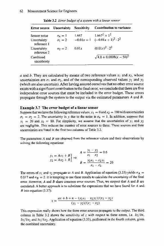
Table 3.2 Error budget o f a system with a linear sensor
Error source Uncertainty Sensitivity Contribution to variance
Sensor noise Uncertainty
reference 1
Uncertainty reference 2
Combined uncertainty
o'n = 1 1.667 1.6672 • 12
o'1 ' - 2 -0 .01x + 1 ( -0 .01x q- 1) 2. 22
o'2 = 2 0.01x (0.01x) 2 �9 22
x/4.8 + 0.0008(x - 50) 2
a and b. They are calculated by means o f two reference values X l and x2, whose
uncer ta int ies are o'1 and 0"2, and o f the cor responding observed values yl and y2 (which are also uncertain) . After hav ing assured ourselves that no other error source
exists wi th a signif icant cont r ibut ion to the final error, we conclude that there are five
independen t error sources that mus t be inc luded in the error budget . These errors
propaga te th rough the sys tem to the output via the es t imated parameters A and B.
Example 3.7 The error budget of a l inear sensor Suppose that we have the following reference values: X 1 = 0 andx2 = 100 with uncertainties
o-1 = o2 = 2. The uncertainty in y due to the noise is o'n = 1. In addition, suppose that
Yl = 20 and Y2 = 80. For simplicity, we assume that the uncertainties of Yl and Y2 are negligible. This reduces the number of error sources to three. These sources and their
uncertainties are listed in the first two columns of Table 3.2.
The parameters A and B are obtained from the reference values and their observations by
solving the following equations:
Yl = A x l + B } y2 = Ax2 + B =~
yl - y2 A = = 0 . 6
Xl -- x2
n y2xl - x2Yl __ 20 Xl - x2
The errors of x 1 and x 2 propagate to A and B. Application of equation (3.33) yields o-A ----
0.017 and o-B "- 2. It is tempting to use these results to calculate the uncertainty of the final
error. However, A and B share common error sources. Thus, we suspect that A and B are
correlated. A better approach is to substitute the expressions that we have found for A and
B into equation (3.37):
z -- ax + b + n - (y2xl - x 2 Y l ) / ( X l - x2)
(Yl -- Y2)/(Xl -- x2)
This expression really shows how the three error sources propagate to the output. The third column in Table 3.2 shows the sensitivity of z with respect to these errors, i.e. a z / a n ,
Oz/Oxl and az/Ox2. Application of equation (3.33), performed in the fourth column, gives
the combined uncertainty.
Measurement Errors and Uncertainty 63
3.5. Characterization of errors
The purpose of this section is to distinguish between the different types of errors that can occur in a measurement. A first dichotomy arises from the distinction between s y s t e m a t i c and r a n d o m errors (Section 3.5.1). A second dichotomy is according to whether the measurement is static or dynamic. Section 3.5.2 discusses some aspects ofthe dynamic case. Section 3.5.3 is an inventory of all kinds ofphysical phenomena that causes different types of errors. Section 3.5.4 is about the specifications of errors.
3.5.1. Sys temat ic errors and random errors
Usually, the error of a measurement is composed of two components, which together are responsible for the combined uncertainty of the measurement. One component is the s y s t e m a t i c e r r o r . The other is the r a n d o m e r r o r . A random error is an error that can be reduced by averaging the results of repeated measurements. The systematic error is the error that persists even after averaging an infinite number of repeated measurements. Thus, we have:
measurement error - systematic error + random error
Once a systematic error is known, it can be quantified, and a correction can be applied. An example of that is recalibration. However, the determination of a cor- rection factor always goes with some uncertainty. In other words, the remainder of a corrected systematic error is a c o n s t a n t r a n d o m e r r o r . Such an error is c o n s t a n t
because if the measurement is repeated, the error does not change. At the same time the error is also r a n d o m because if the calibration is redone, it takes a new value. Hence, the remainder of a corrected systematic error is still a systematic error. Its uncertainty should be accounted for in the combined uncertainty of the measurement.
Example 3.8 Error types of a linear sensor In order to illustrate the concepts, we consider the errors of the linear sensor discussed in example 3.7. The output of the system is (see equation (3.37)):
a x + b + n - B z = (3.38)
A
a and b are two sensor parameters. A and B are two parameters obtained from a two-point calibration procedure. Deviations of A and B from a and b give rise to two systematic errors.
AB AA 1 z ~, x - - x + - �9 n o i s e (3.39)
a a a
I II III
64 Measurement Science for Engineers
The error budget of z consists of three factors:
I a constant, additive random error due to the uncertainty in B II a constant, multiplicative random error due to the uncertainty in A
III an additive, fluctuating random error due to the noise tenn.
According to Table 3.2, the non-constant random error brings an uncertainty of 1.667. The two constant random errors are not independent because they both stem from the calibration error. The uncertainty of the total constant random error is ~/[2 + 0.0008(x - 50)2].
A systematic effect that is not recognized as such leads to unknown systematic errors. Proper modelling of the physical process and the sensor should identify this kind of effect. The error budget and the sensitivity analysis, as discussed in Section 3.4.3, must reveal whether potential defects should be taken seriously or not.
Another way to check for systematic errors is to compare some measurement results with the results obtained from alternative measurement systems (that is, systems that measure the same measurand, but that are based on other principles). An example is the determination of the position of a moving vehicle based on an accelerometer. Such a sensor essentially measures acceleration. Thus, a double integration of the output of the sensor is needed to get the position. Unfortunately, the integrations easily introduce a very slowly varying error. By measuring the position now and then by means of another principle, for instance GPS, the error can be identified and corrected.
In order to quantify a systematic error it is important to define the repeatability conditions carefully. Otherwise, the term "systematic error" is ambiguous. For instance, one can treat temperature variations as a random effect, such that its influence (thermal drift) leads to random errors. One could equally well define the repeatability conditions such that the temperature is constant, thus letting temperature effects lead to a systematic error.
3.5.2. Signal characterization in the time domain
In this section, the context of the problem is extended to a dynamic situation in which measurement is regarded as a process that evolves in time. The measurand is a signal instead of a scalar value. Consequently, the measurement result and the measurement error now also become signals. They are functions of the time t:
e(t) = z( t ) - x ( t ) (3.40)
The concept of a random variable must be extended to what are called stochastic processes (also called random signals). The stochastic experiment alluded to in Section 3.2 now involves complete signals over time, where the time t is defined in some interval. Often this interval is infinite, as in t e ( - c~ , oo), or in t 6 [0, ~ ) .
Measurement Errors and Uncertainty 65
The outcome of a trial is now a signal instead of a number. Such a generated signal is called a realization. After each trial, a so-called stochastic process e(t) takes the produced realization as its new signal. The set of all possible realizations is the ensemble.
If the ensemble is finite (that is, there is only a finite number of realizations to choose from), we could define the probability that a particular realization is generated. However, the ensemble is nearly always infinite. The probability of a particular realization is then zero.
We can bypass this problem by freezing the time to some particular moment t, and by restricting our analysis to that very moment. With frozen time, the stochastic process e(t) becomes a random variable. By that, the concept of a probability density function fe(t)(e, t) of e(t) is valid again. Also, parameters derived from
fe(t)(e,t), such as expectation (=mean)/z(t) and variance 0,2 (t) can then be used.
In principle, fe(t)(e, t) is a function not only of e, but also of t. Consequently,
/z(t) and 0,2(t) depend on time. In the special case, where fe(t)(e, t) and all other
probabilistic parameters 3 of e(t) do not depend on t, the stochastic process e(t) is called stationary.
Often, a non-stationary situation arises when the integration of a noisy signal is involved. A simple example is the measurement of a speed v(t) by means of an accelerometer. Such a sensor actually measures the acceleration a(t) = ~)(t). Its output is y(t) = a(t) + e(t) where e(t) models the errors produced by the sensor, e.g. noise. In order to measure the speed, the output of the accelerometer has to be integrated: z(t) = f y(t) dt = v(t) + C + f e(t)dr . The measurement error is C + f e(t) dt, where C is an integration constant that can be neutralized easily. The second term f e(t) dt is integrated noise. It can be shown [2] that the variance of integrated noise is proportional to time. Therefore, if e(t) is stationary noise with standard deviation ae, the standard deviation of the error in z(t) is kae~/t. The standard deviation grows continuously. This proceeds until the voltage clips against the power supply voltage of the instrumentation.
As said before, stationary random signals have a constant expectation # and a con- stant standard deviation a. Loosely phrased, the expectation is the non-fluctuating part of the signal. The standard deviation quantifies the fluctuating part. The power of an electrical random signal s(t) that is dissipated in a resistor is proportional to E{s_2(t)} = /z 2 + 0 "2. Hence, the power of the fluctuating part and the non- fluctuating part add up. The quantity E{s_2(t)} is called the mean square of the signal. The RMS (root mean square) of a random signal is the square root of the
3 The complete characterization of a stochastic process (in probabilistic sense) does involve much more than that what is described by fe(t)(e,t) alone [2]. However, such a characterization is beyond the scope of this book.
66 Measurement Science for Engineers
mean square:
RMS = v/E{s2(t)} (3.41) g
A true RMS-voltmeter is a device that estimates the RMS by means of averaging over time. Suppose that s(t) is a realization of a stationary random signal, then the output of the RMS-voltmeter is:
~ T f t RMS(t) = s2(r) d r (3.42) =t-T
Ifu( t ) is a periodic signal with period T, that is u(t) = u(t - T), then we can form a stationary random signal by randomizing the phase of u(t). Let r__ be a random variable that is uniformly distributed between 0 and T. Then s(t) = u(t - r__) is a stationary random signal whose RMS is given by equation (3.42).
Example 3.9 RMS of a s inusoidal waveform and a block wave Suppose that s(t) is a sinusoidal waveform with amplitude A and period T and random phase, e.g. s(t) = A sin(2zr(t - r_)/T). Then, the RMS ofs(t) is:
R~4S= V / 1 L O (Asin (2:-r T ) ) 2 A
dt --- (3.43) 4~
If s(t) is a periodic block wave whose value is either +A or -A, the RMS is simply A. Note that the true RMS-voltmeter from equation (3.42) only yields the correct value if the averaging time equals a multiple of the period of the waveform.
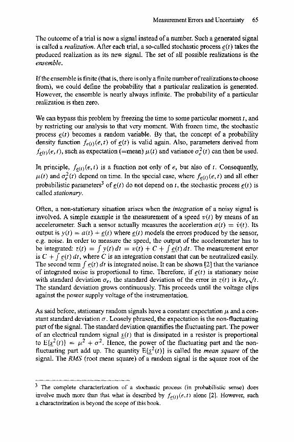
The RMS is a parameter that roughly characterizes the magnitude of a random signal, but it does not characterize the time dependent behaviour. Figure 3.6 shows
(a)
(b)
(c)
i | | |
I I I I
t | ! , |
I I I I
t
t
Figure 3.6 Different types of noise: (a) narrow band noise; (b) low frequency noise," (c) broad band noise
Measurement Errors and Uncertainty 67
three different types of noise. In Figure 3.6(a) the noise has a preference frequency. In fact, this type of noise can be regarded as the sum of a number of harmonics (sinusoidal waveforms) with random amplitudes and phases, but with frequencies that are close to the preference frequency. This type of noise is called narrow band noise, because all frequencies are located in a narrow band around the preference frequency. The noise in Figure 3.6(b) is slowly varying noise. It can be regarded as the sum of a number of harmonics whose frequencies range from zero up to some limit. The amplitudes of these harmonics are still random, but on an average, the lower frequencies have larger amplitudes. It is so-called low frequency noise. The noise realization shown in Figure 3.6(c) is also built from harmonics with frequencies ranging from zero up to a limit. But here, on an average, the amplitudes are equally distributed over the frequencies.
These examples show that the time dependent behaviour can be characterized by assuming that the signal is composed of a number of harmonics with random amp- litudes and random phases, and by indicating how, on average, these amplitudes depend on the frequency. The function that establishes that dependence is the so- called power spectrum P ( f ) where f is the frequency. The power spectrum is defined such that the power (= mean square; see page 66) of the signal measured in a small band around f and with width A f is P ( f ) A f .
The term white noise refers to noise which is not bandlimited, and where, on an average, all frequencies are represented equally. In other words, the power spectrum of white noise is flat: P ( f ) -- Constant . Such a noise is a mathem- atical abstraction, and cannot exist in the real world. In practice, if the power spectrum is flat within a wide band, such as in Figure 3.6(c), it is already called "white".
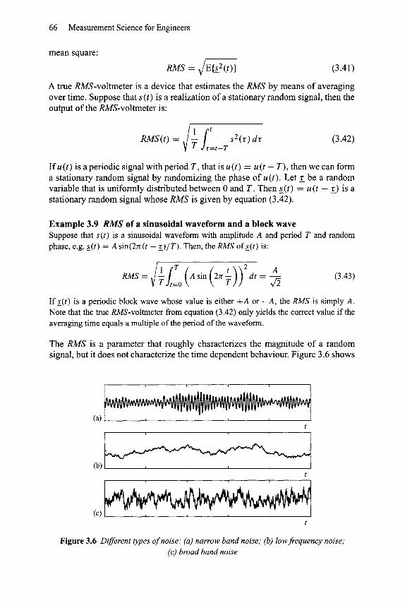
Example 3.10 Noise characterization of an amplifier Figure 3.7 shows the model that is used to characterize the noise behaviour of an amplifier. Such a device is used to amplify the signal generated by a sensor, here modelled by a voltage Vi and a resistor R. The output of the amplifier is Vo. The noise produced by the amplifier is modelled with two noise sources, a voltage source Vn and a current source In. These sources are at the input side of the amplifier.
Figure 3.7 The noise characterization of an amplifier
68 Measurement Science for Engineers
The manufacturer specifies the square root of the power density at a given frequency. For instance, the LM6165 is a high speed, low noise amplifier. The noise specifications are: Vn = 5 nV/~I-Iz and In = 1.5pA/~1-Iz measured at f = 10kHz. In fact, these figures are the RMSs of the noise voltage and current if the bandwidth of the amplifier was 1 Hz centred around 10 kHz. In other words, the power spectra at f = 10 kHz is Pen (10 kHz) = 25 (nV) 2/Hz and Pin (10 kHz) = 2.25 (pA) 2/Hz.
If the noise is white, then the noise spectra are flat. Thus, Pvn ( f ) = Cvn with Cvn = 25 (nV)2/Hz and Pin ( f ) = Cln with Cln = 2.25 (pA)2/Hz. Suppose that the bandwidth of the amplifier is B, then the noise power is BCVn and BCvn. For instance, if B = 10 MHz, then the power is 2.5 • 10-10V 2 and 2.25 • 10 -17 A 2, respectively. The RMSs are the
square root of that: 16 IxV and 5 nA.
Most amplifiers show an increase of noise power at lower frequencies. Therefore, if the bandwidth of the amplifier encompasses these lower frequencies, the calculations based on the "white noise assumption" are optimistic.
3.5.3. Error sources
The uncertainties in measurement outcomes are caused by physical and technical constraints. In order to give some idea of what effects might occur, this section mentions some types of error sources. The list is far from complete.
Systematic effects
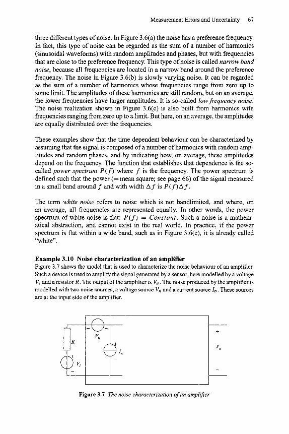
Saturation, dead zone, hysteres& These phenomena are characterized by a static, nonlinear mapping of the measurand x and the output of a sensor: y = g(x). The effects are illustrated in Figure 3.8. Saturation occurs when the sensitivity Og/Ox decreases as Ixl increases (see Figure 3.8(a)). If Ix l becomes too large, y clips against the power voltage or ground. The dead zone of a sensor is an interval of x for which the output of the sensor does not change. In a mechanical system, static friction (called stiction) could be the cause. Stiction forms a barrier that a force must overcome before the relative motion of two bodies in contact can begin. Hysteresis is characterized by the phenomenon that g(x) depends on whether x is increasing or decreasing.
J (a)
X
Figure 3.8 Non-linear systematic errors

Measurement Errors and Uncertainty 69
It occurs in mechanical systems when two parts have a limited space for free movement.
Loading errors A loading error occurs when the interaction between the physical process and the sensor is not compensated. A well-known example is the measurement of the potential difference over a resistor by means of a voltmeter. The internal impedance of the voltmeter influences this potential difference, and thus, without compensation, an error occurs.
Another example is the measurement of the temperature in a furnace. The tem- perature sensor is located either in the wall of the furnace, or outside the furnace connected to a thermal conductor. Due to thermal leakage, there will be a temperature difference between the centre of the furnace and the sensor.
Example 3.11 Loading error of a voltmeter Figure 3.9 shows a model of a sensor with output voltage Vy and internal resistor R connected to the input of a voltmeter. The input voltage Vi of the voltmeter is affected by its input impedance Ri :
R/ ( ~ / ) Vi = Ri + R VY ~" 1 - Vy (3.44)
The approximation is accurate if R i >> R. Clearly, the load of the sensor can cause a systematic error that must be compensated (see Section 7.1).
Calibration errors Calibration errors are induced by:
�9 The uncertainty of the reference values (the conventional true values) (see Example 3.7).
�9 Random errors that occur during calibration. �9 Erroneous calibration curves.
R
ivy
i + i vi
Figure 3.9 The loading error of a voltmeter
70 Measurement Science for Engineers
Errors in a two-point calibration procedure lead to a multiplicative and an additive error. See Example 3.8. A wrong calibration curve occurs when a two-point calib- ration procedure is used based on a linear model of the sensor, whereas in reality the sensor is nonlinear. A solution might be to use some polynomial as a calibration curve, and to fit that curve using multiple-point calibration.
Dynamic errors
Dynamic errors occur when the measurement instrument is too slow to be able to keep track of a (fast changing) measurand. The change of the output of an amplifier is limited. This is one cause of a dynamic error.
Another dynamic error occurs when the bandwidth of the instrument is not suffi- cient. The measuring device should have an amplitude transfer that is constant over the full bandwidth of the measurand. In that region, the phase characteristic should hold a linear relationship with the frequency.
In time-discrete systems, a too low sampling frequency gives rise to aliasing errors (see Chapter 5).
Random effects
Environmental errors
External influences may cause errors that are often random. An example is electro- magnetic interference (EMI). The interfering noise with power concentrated at multiples of 50 (or 60) Hz often originates from the mains of the AC power supply. Pulse-like interferences occur when high voltages or currents are switched on or off. These types of interferences are caused by electrical discharges in a gas (e.g. as in the ignition system of a petrol engine) or by the collector of an AC electromotor. At much higher frequencies, EMI occurs, for instance, from radio stations.
Resolution error
The resolution error is the generic name for all kinds of quantization effects that might occur somewhere in the measurement chain. Examples are:
�9 A wire wound potentiometer used for position measurement or for attenuation. �9 A counter used for measuring distances (i.e. an odometer). �9 AD converters. �9 Finite precision arithmetic.
Essentially, the resolution error is a systematic error. However, since the resolution error changes rapidly as the true value changes smoothly, it is often modelled as a random error with a uniform distribution function.

Measurement Errors and Uncertainty 71
Drift The genetic name for slowly varying, random errors is drift. Possible causes for drift are: changes of temperature and humidity, unstable power supplies, 1 / f noise (see below), and so on.
Noise The generic name for more or less rapidly changing, random errors is noise. The thermal noise (also called Johnson noise) of a resistor is caused by the random, thermal motion of the free electrons in conductors. In most designs, this noise can be considered as white noise, because the power spectrum is virtually flat up to hundreds of MHz. The mechanical equivalent of Johnson noise is the so-called Brownian motion of free particles in a liquid.
Another physical phenomenon that is well described by white noise is the so-called Poisson noise or shot noise. It arises from the discrete nature of physical quantities, such as electrical charge and light. For instance, in a photodetector, light emitted on a surface is essentially a bombardment of that surface by light photons. The number of photons received by that surface within a limited time interval has a Poisson distribution.
Some noise sources have a power spectrum that depends on the frequency. A well- known example is the so-called 1 / f noise. It can be found in semiconductors. Its power spectrum is in a wide frequency range inversely proportional to some power of the frequency, i.e. proportional to 1 / fp where p is in the range from 1 to 2.
3.5.4. Specifications
The goal of this section is to explain the generally accepted terms that are used to specify sensor systems and measurement instruments.
Sensitivity, dynamic range and resolution The sensitivity S of a sensor or a measurement system is the ratio between output and input. If z = f ( x ) , then the sensitivity is a differential coefficient S = Of/Ox evaluated at a given set point. If the system is linear, S is a constant.
The range of a system is the interval [Xmin , X m a x ] in which a device can measure the measurand within a given uncertainty ae. The dynamic range D is the ratio D = (Xmax - Xmin)/O'e. Often, the dynamic range is given on a logarithmic scale in dB. The expression for that is D = 20 101og[(Xma x - - Xmin)/O'e].
The resolution R expresses the ability of the system to detect small increments of the measurand. This ability is limited due to the resolution errors, dead zones and hysteresis of the system. The resolution is defined as R = x / A x where Ax is the
72 Measurement Science for Engineers
smallest increment that can be detected. Often, the specification is given in terms of maximum resolution: Rmax = Xmax/Ax.
Accuracy, repeatability and reproducibility The accuracy is the closeness of agreement between the measurement result and the true value. The quantification of the accuracy is the uncertainty, where uncertainty comprises both the random effects and the systematic effects.
The repeatability is the closeness of agreement between results of measurement of the same value of the same measurand, and which are obtained under the same conditions (same instrument, same observer, same location, etc.). Hence, the repeat- ability relates to random errors, and not to systematic errors. The quantification is the uncertainty, where uncertainty comprises only the random effects.
The reproducibility is the closeness of agreement between results of measurements of the same value of the same measurand, but that are obtained under different con- ditions (different instruments, different locations, possibly different measurement principles, etc.).
Offset, gain error and nonlinearity If z = g(x), then the offset error (or zero error) is AA = g(0). The offset is an additive error. The gain error A B in a linear measurement system, z = B x, is the deviation of the slope from the unit value: AB = B - 1. The gain error gives rise to a multiplicative error x A B.
The nonlinearity error is g(x ) - A - B x where A and B are two constants that can be defined in various ways. The simplest definition is the end point method. Here, A and B are selected such that g(Xmin) = A + Bxmin and g(Xmax) = A + Bxmax. Another definition is the best f i t method. A and B are selected such that A + B x fits g(x ) according to some closeness criterion (e.g. a least squares error fitting). The nonlinearity is the maximum nonlinearity error observed over the specified range expressed as a percentage ofthe range L = max(Ig(x) - A - Bxl)/(Xmax - Xmin). These concepts are illustrated in Figure 3.10.
Bandwidth, indication time and slew rate These are the three most important parameters used to characterize the dynamic behaviour. The bandwidth is the frequency range in which a device can measure. Usually, it is defined as the frequency range for which the transfer of power is not less than half of the nominal transfer. If H ( f ) is the (signal) transfer function, and H ( f ) = 1 is the nominal transfer, then halfofthe power is transferred at frequencies for which [H (f)]2 = 1. The cut-off frequency fc follows from [H (fc)[ = 1/~/2 which corresponds to - 3 dB with respect to the nominal response. The response for zero frequency (i.e. steady state) is for most systems nominal. For these systems, the bandwidth equals re. Obviously, for systems with a band-pass characteristic, two cut-off frequencies are needed.

Measurement Errors and Uncertainty 73
g(x) 0 . 5
end point fit ~ . " . . ' "
| i
1 2 x
nonlinearity error
�9 4- lse fit .
�9
,.
*
o o
�9 , . �9 . . " ~ 1 7 6 1 4 9 ."
�9 .~--- end point fit .-
.
0 --0.5 0 0 1 2 x
Figure 3.10 Nonlinearity errors
- 5 - 1
I - - v 'It "T 'W ~ w ' v ' w - ~ ' ' w r ' ' ' n ' - response time - -~
I I I I I
0 1 2 3 t 4
F i g u r e 3 .11 Response time
The indication time or response time is the time that expires from a steplike change of the input up to the moment that the output permanently enters an inter- val [z0 - Az, z0 + Az] around the new steady state z0. For Az, one chooses a multiple of the uncertainty (see Figure 3.11).
The slew rate is the system's maximum change rate of output max[Idz/dtl] .
C o m m o n mode rejection ratio It often occurs that the measurand is the difference between two physical quantities: Xd = X l -- x2. In the example of Figure 3.12(a), the measurand is the level l of a liquid. The sensor measures the difference between pressures at the surface and at the bottom of the tank. The relation l = (pl - p2)/Pg where p is the mass density can be used to measure I. Other examples are differences between: floating voltages, forces, magnetic flux, etc. Such a measurement is called a differential measurement. The difference xd is the differential mode input. The average of the
74 Measurement Science for Engineers
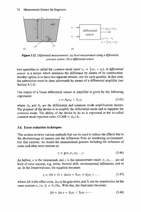
Figure 3.12 Differential measurements: (a) level measurement using a differential pressure sensor; (b) a differential sensor
two quantities is called the common mode input Xc = ) (Xl -~- x2). A differential sensor is a sensor which produces the difference by means of its construction. Another option is to have two separate sensors, one for each quantity. In that case, the subtraction must be done afterwards by means of a differential amplifier (see Section 4.1.4).
The output of a linear differential sensor or amplifier is given by the following expression:
z = AdXd + Acxc (3.45)
where Ad and Ac are the differential and common mode amplification factors. The purpose of the device is to amplify the differential mode and to suppress the common mode. The ability of the device to do so is expressed in the so-called common mode rejection ratio: CCMR = A d / A c .
3.6. Error reduction techniques
This section reviews various methods that can be used to reduce the effects due to the shortcomings of sensors and the influences from an interfering environment. For that purpose, we model the measurement process including the influence of noise and other error sources as:
z -- g (x , el, e2 , . . . ) (3.46)
As before, x is the measurand, and z is the measurement result, el, e2 , . . , are all kind of error sources, e.g. noise, thermal drift, environmental influences, and so on. In the linearized case, the equation becomes:
z = A b + (1 + A a ) x + Slel + $2e2 + . . . (3.47)
where Ab is the offset error, Aa is the gain error, and Si are the sensitivities for the error sources ei, i.e. Si = Oz/Oei. With that, the final error becomes:
A b + A a x + Sle l + $2e2 + . . . (3.48)

Measurement Errors and Uncertainty 75
This expression shows that the error is composed of two parts. The first part is the calibration error Ab + Aa x. It can be minimized by a proper calibration proced- ure, or by application of feedback (see Section 3.6). Due to ageing and wear, the transformation characteristic, a and b, may change over time. Therefore, now and then, the system needs recalibration. Smart sensor systems have built-in facilities that enable automatic recalibration even during operation. If the transformation characteristic is nonlinear, a correction curve should be applied. The parameters of this curve should also be refreshed by recalibration.
The second part, Slel d-- $2e2 + . . . , is the result of the errors that are induced somewhere in the measurement chain, and that propagate to the output. Each term of this part consists of two factors: the error sensitivity Si and the error source ei. Essentially, there are three basic methods to reduce or to avoid this type of error [4]:
�9 Elimination of the error source ei itself. �9 Elimination of the error sensitivity Si. �9 Compensation of an error term Si ei by a second term -S i ei.
These techniques can be applied at the different stages of the measurement process. Preconditioning is a collection of measures and precautions that are taken before the actual measurement takes place. Its goal is either to eliminate possible error sources, or to eliminate their sensitivity coefficients. Postconditioning orpostprocessing are techniques that are applied afterwards. The compensation techniques take place during the actual measurement.
The following sections present overviews of these techniques.
3.6.1. Elimination o f error sources
Obviously, an effective way to reduce the errors in a measurement would be to take away the error source itself. Often, the complete removal is not possible. How- ever, a careful design of the system can already help to diminish the magnitude of many of the error sources. An obvious example is the selection of the electronic components, such as resistors and amplifiers. Low-noise components must be used for those system parts that are most sensitive to noise (usually the part around the sensor).
Another example of error elimination is the conditioning of the room in which the measurements take place. Thermal drift can be eliminated by stabilizing the temperature of the room. If the measurement is sensitive to moisture, then the regularization of the humidity of the room might be useful. The influence of air and air pressure is undone by placing the measurement set up in vacuum. Mechanical vibrations and shocks are eliminated for a greater part by placing the measurement set up in the basement of a building.
76 Measurement Science for Engineers
3.6.2. Elimination o f the error sensitivities
The second method to reduce errors is blocking the path from error source to measurement result. Such can be done in advance, or afterwards. Examples of the former are:
�9 Heat insulation of the measurement set up in order to reduce the sensitivity to variations of temperature.
�9 Mounting the measurement set up on a mechanically damped construction in order to reduce the sensitivity to mechanical vibrations, i.e. a granite table top resting on shock absorbing rubbers.
�9 Electronic filtering before any other signal processing takes place. For instance, prefiltering before AD-conversion (Chapter 6) can reduce the noise sensitivity due to aliasing. Electronic filters are discussed in Section 4.2.
Postfiltering An example of reducing the sensitivity afterwards is postfiltering. In the static situation, repeated measurements can be averaged so as to reduce the random error. If N is the number of measurements, then the random error of the average reduces by a fraction 1~siN (see equation (3.18)).
In the dynamic situation z(t) is a function oftime. The application of a filter is ofuse if a frequency range exists with much noise and not much signal. Therefore, a filter for noise suppression is often a low-pass filter or a band-pass filter. Section 4.2 discusses the design of analogue filters. Here, we introduce the usage of digital filters.
Suppose that the measurements are available at discrete points of time tn = nAT , as in digital measurement systems. This gives a time sequence of measurement samples z(nAT) . We can apply averaging to the last N available samples. Hence, if n A T denotes the current time, the average over the last N samples is:
1 N - 1
~(nAT) = -~ ~ z ((n - re)AT) m=O
(3.49)
Such a filter is called a moving average filter (MA-filter). The reduction of random errors is still proportional to 1/x/N. Often, however, the random errors in successive samples are not independent. Therefore, usually, moving averaging is less effective than averaging in the static case.
For the reduction of random errors it is advantageous to choose N very large. Unfortunately, this is at the cost of the bandwidth of the measurement system. In the case of MA-filtering the cut-off frequency of the corresponding low-pass filter is inversely proportional to the parameter N. If N is too large, not only the noise is suppressed, but also the signal.

Measurement Errors and Uncertainty 77
There are formalisms to design filters with optimal transfer function. Such a filter yields, for instance, maximum signal-to-noise ratio at its output. Examples of these filters are the Wiener filter and the Kalman filter [2].
Guarding and grounding As mentioned in Section 3.5.3, many external error sources exist that cause an electric or magnetic pollution of the environment of the measurement system. Without countermeasures, these environmental error sources are likely to enter the system by means of stray currents, capacitive coupling of electric fields, or inductive coupling of magnetic fields. The ground of an electric circuit is a con- ducting body, such as a wire, whose electric potential is - by convent ion- zero. However, without precautions, the ground is not unambiguous. The environmental error sources may induce stray currents in the conductors of the electric circuits, in the metallic housing of the instrumentation, or in the instrumental racks. Guarding is the technique of grounding a system, such that these stray currents do not occur, or do not enter the system.
The earth of the mains power usually consists of a connection to a conducting rod which is drilled into the ground such that the impedance between rod and earth is smaller than 0.2 f2. Unfortunately, the potential difference between two earths from two main plugs can be substantial because of the environmental error sources. Therefore, it is not appropriate to consider both earths as one ground. One can define one of the earths of these plugs as the ground of the system, but it is not necessary (and sometimes undesirable) to do so. In fact, the main reason for having an earth is the safety that it offers when connected to the housings of the instruments 4.
As an example, Figure 3.13(a) shows an instrumentation system with two electrical connections to earth points. Such a configuration induces disturbances that can- not be fully compensated by a differential amplifier. The disturbances arise from stray currents that always exist between different earth points. The impedance R A between the two earth points is on the order of 0.1 f2. Together with the stray currents, it forms a potential difference between the earth points. The potential dif- ference is largely a common mode disturbance. Therefore, it will be compensated
(a) .................................. ~ i Vt~AM.j
R1 R1 v-n v---1
R2 v--3
RA r-----]
.................................... i
,!n n!i (b)
sensor .....................................
R2 c---1
Ri Ol Vi
Figure 3.13 Grounding: (a) creation of a ground loop by two earth points; (b) star point grounding
4 Many instruments have a terminal marked with "earth" or I . Such a terminal is connected to the housing of the instruments and can be connected to the earth.
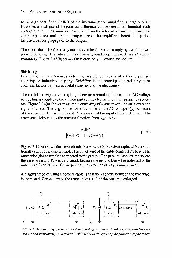
78 Measurement Science for Engineers
for a large part if the CMRR of the instrumentation amplifier is large enough. However, a small part of the potential difference will be seen as a differential mode voltage due to the asymmetries that arise from the internal sensor impedance, the cable impedance, and the input impedance of the amplifier. Therefore, a part of the disturbances propagates to the output.
The errors that arise from stray currents can be eliminated simply by avoiding two- point grounding. The rule is: never create ground loops. Instead, use star point grounding. Figure 3.13(b) shows the correct way to ground the system.
Shielding Environmental interferences enter the system by means of either capacitive coupling or inductive coupling. Shielding is the technique of reducing these coupling factors by placing metal cases around the electronics.
The model for capacitive coupling of environmental inferences is an AC voltage source that is coupled to the various parts of the electric circuit via parasitic capacit- ors. Figure 3.14(a) shows an example consisting of a sensor wired to an instrument, e.g. a voltmeter. The ungrounded wire is coupled to the AC voltage VAc by means of the capacitor Cp. A fraction of VAc appears at the input of the instrument. The error sensitivity equals the transfer function from VAc to Vi:
RsllRi
[(gsllg) + [(1/(jogCp)][ (3.50)
Figure 3.14(b) shows the same circuit, but now with the wires replaced by a rota- tionally symmetric coaxial cable. The inner wire of the cable connects Rs to Ri. The outer wire (the coating) is connected to the ground. The parasitic capacitor between the inner wire and VAc is very small, because the ground keeps the potential of the outer wire fixed at zero. Consequently, the error sensitivity is much lower.
A disadvantage of using a coaxial cable is that the capacity between the two wires is increased. Consequently, the (capacitive) load of the sensor is enlarged.
I i
c~ II
VAc v~~ " ~ sensor
. . . . . . . . . . . . . . . . . . . . . . . . . . . . . . . . . . . . .
(a) (b)
!ns en
c~ II
i sensor
Coax cable
m
Figure 3.14 Shielding against capacitive coupling: (a) an unshielded connection between sensor and instrument; (b) a coaxial cable reduces the effect of the parasitic capacitance

Measurement Errors and Uncertainty 79
Figure 3.15 Shielding against inductive coupling: (a) a changing magnetic field induces a voltage in the loop area created by the two connecting wires; (b) a twisted cable reduces
the inductive coupling
Example 3.12 The sensitivity of an unshielded input lead Suppose that the parasitic capacity per unit length of a wire is 5 pF/m. The length of the wire is 1 m. The RMS of the error source is VAC = 220 V at a frequency of 50 Hz. Rs = 1 O0 ~2. The input impedance of the instrument is large compared with Rs. The RMS voltage of the error at the input of the instrument is 35 IxV. If with coaxing the remaining capacitance can be reduced to 0.05 pF, the error will be 0.35 IxV.
Induction is another mechanism for coupling to environmental interferences. Magnetic fields are caused by large currents in the neighbourhood of the meas- urement set-up. A magnetic field induces a voltage in a loop area of a wire according to:
d ~ /~.d-~ (3.51) Vmag = dt tea
Figure 3.15(a) illustrates an example. Here, the connecting wires between a sensor and the instrument forms a loop with area A.
The coupling can be reduced in the following ways:
�9 Shielding the wires by metal cases.
�9 Arranging the geometry of the wiring such that B _1_ dA. �9 Minimizing the loop area.
Shielding the wires is not always very effective because for most metals the penet- ration depth of a magnetic field is large (except for mumetal). The second solution is also difficult because the direction of the magnetic field is often unknown. The third solution is often applied. The wires in a cable are often twisted in order to alternate the sign of the magnetic field across the loop area (see Figure 3.15(b)). Another possibility is to use coaxial cable. Here, the loop area is zero because of the rotationally symmetry.
3.6.3. Compensation
Here, we accept that an error enters the system and propagates to the output, yielding Siei. The strategy is to add another term - S i e i that compensates Siei. This principle
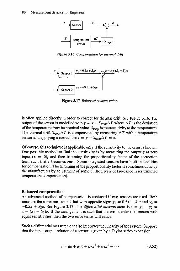
80 Measurement Science for Engineers
x ~1 Sensor I ] I
T J temperature sensor
y
AT "q~[ -Stemp I
Figure 3.16 Compensation for thermal drift
Sensor 1 ] yl= 0.5x +Sle .J"'x
Sensor 2 + Sze
z = x + (S l - S2)e i v
Figure 3.17 Balanced compensation
is often applied directly in order to correct for thermal drift. See Figure 3.16. The output of the sensor is modelled with y = x + StempAT where AT is the deviation of the temperature from its nominal value. Stemp is the sensitivity to the temperature. The thermal dritt StempAT is compensated by measuring AT with a temperature sensor and applying a correction: z = y - S term A T = x.
Of course, this technique is applicable only if the sensitivity to the error is known. One possible method to find the sensitivity is by measuring the output z at zero input (x = 0), and then trimming the proportionality factor of the correction term such that z becomes zero. Some integrated sensors have built-in facilities for compensation. The trimming of the proportionality factor is sometimes done by the manufacturer by adjustment of some built-in resistor (so-called laser trimmed temperature compensation).
Balanced compensation An advanced method of compensation is achieved if two sensors are used. Both measure the same measurand, but with opposite sign: yl = 0.5x + S1 e and Y2 = -0 .5x + S2e. See Figure 3.17. The differential measurement is z = Yl - Y2 = x + (S1 - S2)e. If the arrangement is such that the errors enter the sensors with equal sensitivities, then the two error terms will cancel.
Such a differential measurement also improves the linearity of the system. Suppose that the input-output relation of a sensor is given by a Taylor series expansion
y = ao + alx + a2x 2 + a3 x3 -b . . . (3.52)
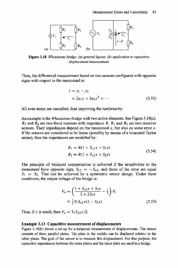
Measurement Errors and Uncertainty 81
R1 R 3
*W'o RE (a) R4 (b)
C1 ] ~ ~_~. R3
= ~ x - d ~ R4
Figure 3.18 Wheatstone bridge: (a) general layout (b) application to capacitive displacement measurement
Then, the differential measurement based on two sensors configured with opposite signs with respect to the measurand is:
z = Yl --Y2
= 2alx + 2a3x 3 + . . . (3.53)
All even terms are cancelled, thus improving the nonlinearity.
An example is the Wheatstone bridge with two active elements. See Figure 3.18(a). R3 and R4 are two fixed resistors with impedance R. R1 and RE are two resistive sensors. Their impedances depend on the measurand x, but also on some error e. If the sensors are considered to be linear (possibly by means of a truncated Taylor series), then the impedances are modelled by:
R1 = R(1 + SxlX + Sle)
R2 = R(1 + Sx2x + S2e) (3.54)
The principle of balanced compensation is achieved if the sensitivities to the measurand have opposite sign, Sxl -- -Sx2, and those of the error are equal S1 --- $2. That can be achieved by a symmetric sensor design. Under these conditions, the output voltage of the bridge is:
1 + Sx2x + Sle 1) Vo = 2 + 2S1 e 2
"~ 1ViSx2x(1 - Sle) (3.55)
Thus, if x is small, then Vo = Vi Sx2x/2.
Example 3.13 Capacitive measurement of displacements Figure 3.18(b) shows a set-up for a balanced measurement of displacements. The sensor consists of three parallel plates. The plate in the middle can be displaced relative to the other plates. The goal of the sensor is to measure this displacement. For that purpose, the capacitive impedances between the outer plates and the inner plate are used in a bridge.
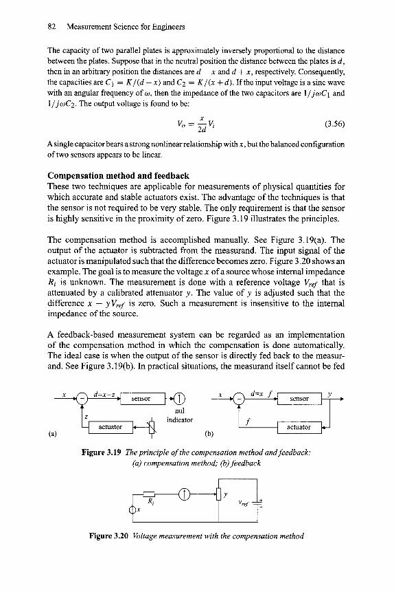
82 Measurement Science for Engineers
The capacity of two parallel plates is approximately inversely proportional to the distance between the plates. Suppose that in the neutral position the distance between the plates is d, then in an arbitrary position the distances are d - x and d + x, respectively. Consequently, the capacities are C1 = K/ (d - x) and C2 = K / ( x + d). If the input voltage is a sine wave with an angular frequency of o9, then the impedance of the two capacitors are 1/jogC1 and 1/jogC2. The output voltage is found to be:
x Vo = -~ Vi (3.56)
A single capacitor bears a strong nonlinear relationship with x, but the balanced configuration of two sensors appears to be linear.
Compensation method and feedback These two techniques are applicable for measurements of physical quantities for which accurate and stable actuators exist. The advantage of the techniques is that the sensor is not required to be very stable. The only requirement is that the sensor is highly sensitive in the proximity of zero. Figure 3.19 illustrates the principles.
The compensation method is accomplished manually. See Figure 3.19(a). The output of the actuator is subtracted from the measurand. The input signal of the actuator is manipulated such that the difference becomes zero. Figure 3.20 shows an example. The goal is to measure the voltage x of a source whose internal impedance Ri is unknown. The measurement is done with a reference voltage Vref that is attenuated by a calibrated attenuator y. The value of y is adjusted such that the difference x - y Vref is zero. Such a measurement is insensitive to the internal impedance of the source.
A feedback-based measurement system can be regarded as an implementation of the compensation method in which the compensation is done automatically. The ideal case is when the output of the sensor is directly fed back to the measur- and. See Figure 3.19(b). In practical situations, the measurand itself cannot be fed
(a)
x .,I I,/'T'x x .,f-'h d=x-f.,I l Y ~/"~ d=x-z " ~ "1 sensor ~ nul "k~ ,-1 sensor ~
~ _ ~ indicator f actuator actuator (b)
Figure 3.19 The principle of the compensation method and feedback: (a) compensation method," (b) feedback
@ Y Vref
Figure 3.20 Voltage measurement with the compensation method

Measurement Errors and Uncertainty 83
Figure 3.21 General lay-out of a feedback measurement system
back. Instead, some derived variable Kx is used (see Figure 3.21). In this figure, the actuator itself is represented by A. In addition, we have two design paramet- ers G and B. The factor G is used to influence the feedback signal. The factor B transforms the sensor signal y to the final measurement result z. The analysis of this system is as follows:
d = Kx - f ] SK y = S d ] y = f = GAy 1 + SGA z = By z = By
(3.57)
If G is selected such that SGA is large, then z = BK(GA)- lx . Thus, a suitable choice of B is K -1GA. Then z = x, and the result does not depend on the actual value of S.
It must be noticed that the subsystems K, S and A depend on the frequency of the measurand x. A stability analysis must be done to find the choices of G that assure a stable system that covers the desired frequency band.
An error source that enters the system atthe output ofthe actuator, i.e. f = GAy+el induces an error at the output o f - e l / K . Thus, the sensitivity of this error is S1 = - 1 / K . An error source that enters the system at the output of the sensor, i.e. y = Sd + e2 induces an error at the output of e2/KS. The sensitivity is 1/KS.
Chapters 7, 8 and 9 present various examples of sensor system in which feedback plays an important role.
3.7. Further reading
[1]
[21
[3]
[4]
A.J. Wheeler, A.R. Ganji, Introduction to Engineering Experimentation, Second Edition, Pearson Prentice-Hall, Upper Saddle River, NJ, 2004. C.F. Dietrich, Uncertainty, Calibration and Probability- The Statistics of Scientific and Industrial Measurement, Second Edition, Adam Hilger, Bristol, 1991. K.S. Shanmugan, A.M. Breipohl, Random Signals, Detection, Estimation and Data Analysis, J. Wiley & Sons, 1988. A. Gelb (editor): Applied Optimal Estimation, M.I.T. Press, Cambridge (Mass.), 1974.

84 Measurement Science for Engineers
[5]
[6]
F. van der Heijden, D. de Ridder, D.M.J. Tax, R.EW. Duin, Classification, Parameter Estimation and State Estimation -An engineering approach using MAT~8, J. Wiley & Sons, Chichester, 2004. A.F.E van Putten, Electronic Measurement Systems: Theory and practice, Second Edition, IOP Publ., 1996.
Some bibliographical notes
The concept of uncertainty is defined formally in a report of the International Organization for Standardization (ISO) [ 1 ]. Wheeler and Ganji's book contains a chapter with detailed coverage of uncertainty analysis. Dietrich's book also pays great attention to uncertainty analysis, but unfortunately this book is less accessible.
There is an overwhelming amount of literature on probability theory, but the book by Papoulis [2] is the classic text. We also mention the book by Shanmugan et al. because of its access- ibility for first- or second-year undergraduate students. The topic of statistical inference is also covered by many textbooks. Kreyszig's book [3] has been selected here because of its accessibility.
The topic of Kalman filtering, i.e. the problem of simultaneously estimating dynamic vari- ables using a multi-sensor system, is covered by Gelb's book, which in this area is considered the "bible". However, the latest developments, such as particle filtering, are not treated. For a more recent introduction of the topic see the book by van der Heijden et al.
The book by van Putten contains chapters about noise sources and about error reduction techniques. It goes into more detail than is possible here.
3.8. Exercises
1. A measurement instrument consists of a sensor/amplifier combination and an AD-converter. The noise at the output of the amplifier has a standard deviation of about 2.0 mV. The quantization step of the AD-converter is 3.00 mV. The AD-converter rounds off to the nearest quantization level. What is the standard uncertainty of the measurement result?
2. A measuring instrument consists of a sensor/amplifier combination and an AD-converter. The sensor/amplifier shows a systematic error with a standard uncertainty of 1 mV. The standard deviation of the noise at the output ofthe amplifier is 1 mV. Both the systematic error and the noise are normally distributed. The quant- ization step of the AD-converter is 1 mV. The AD converter rounds offto the nearest quantization level. What is the approximate distribution of the resulting error, and what is the standard deviation?
3. A measuring instrument consists of a sensor/amplifier combination and an AD-converter. The sensor/amplifier shows a systematic error with a standard uncer- tainty of 0.01 mV. The standard deviation of the noise at the output of the amplifier
Measurement Errors and Uncertainty 85
is 0.01 mV. The quantization step of the AD-converter is 1 mV. The AD converter rounds off to the nearest quantization level. The measurand is static. In order to improve the accuracy, the measurement is repeated 100 times, and the results are averaged. What is the resulting uncertainty?
4. The postal service wants to know the volume of a block shaped parcel. For that purpose the three edges of the parcel are measured with a relative uncertainty of 2%. What is the relative uncertainty of the estimated volume?
5. A cylindrical rain gauge measures the amount of rain by collecting the rain drops. The top area of the gauge is 5 cm 2. After twenty-four hours, the level in the gauge is 2.0 cm. Assume that the mean volume of a rain drop is 0.10 cm 3. What is the standard uncertainty of the level?
6. The length of an object is repeatedly measured with the following results:
8, 8, 9, 7, 6, 8, 9, 8, 6, 7(units: mm)
The results are averaged in order to reduce the random error.
a. What is the estimated mean? b. What is the sample variance of the sequence? c. What is the estimated uncertainty of the mean? d. What is the estimated uncertainty of the sample variance?