Atmos. Meas. Tech., 7, 799–822, 2014www.atmos-meas-tech.net/7/799/2014/doi:10.5194/amt-7-799-2014© Author(s) 2014. CC Attribution 3.0 License.

Atmospheric Measurement

TechniquesO

pen Access

Probabilistic approach to cloud and snow detection on AdvancedVery High Resolution Radiometer (AVHRR) imagery

J. P. Musial1,2,*, F. Hüsler1,2, M. Sütterlin 1,2, C. Neuhaus1,2, and S. Wunderle1,2

1Geographisches Institut der Universität Bern (GIUB), 3012 Bern, Switzerland2Oescher-Zentrum für Klimaforschung, Universität Bern, Zähringerstrasse 25, 3012, Bern, Switzerland* currently at: the Remote Sensing Department, Institute of Geodesy and Cartography, Modzelewskiego 27,02-679 Warsaw, Poland

Correspondence to:J. P. Musial (jan.musial@giub.unibe.ch)

Received: 15 May 2013 – Published in Atmos. Meas. Tech. Discuss.: 25 September 2013Revised: 28 January 2014 – Accepted: 3 February 2014 – Published: 28 March 2014

Abstract. Derivation of probability estimates complemen-tary to geophysical data sets has gained special attentionover the last years. Information about a confidence level ofprovided physical quantities is required to construct an er-ror budget of higher-level products and to correctly inter-pret final results of a particular analysis. Regarding the gen-eration of products based on satellite data a common inputconsists of a cloud mask which allows discrimination be-tween surface and cloud signals. Further the surface informa-tion is divided between snow and snow-free components. Atany step of this discrimination process a misclassification ina cloud/snow mask propagates to higher-level products andmay alter their usability. Within this scope a novel probabilis-tic cloud mask (PCM) algorithm suited for the 1 km× 1 kmAdvanced Very High Resolution Radiometer (AVHRR) datais proposed which provides three types of probability es-timates between: cloudy/clear-sky, cloudy/snow and clear-sky/snow conditions. As opposed to the majority of availabletechniques which are usually based on the decision-tree ap-proach in the PCM algorithm all spectral, angular and ancil-lary information is used in a single step to retrieve probabil-ity estimates from the precomputed look-up tables (LUTs).Moreover, the issue of derivation of a single threshold valuefor a spectral test was overcome by the concept of multidi-mensional information space which is divided into small binsby an extensive set of intervals. The discrimination betweensnow and ice clouds and detection of broken, thin cloudswas enhanced by means of the invariant coordinate system(ICS) transformation. The study area covers a wide range

of environmental conditions spanning from Iceland throughcentral Europe to northern parts of Africa which exhibit di-verse difficulties for cloud/snow masking algorithms. The re-trieved PCM cloud classification was compared to the PolarPlatform System (PPS) version 2012 and Moderate Resolu-tion Imaging Spectroradiometer (MODIS) collection 6 cloudmasks, SYNOP (surface synoptic observations) weather re-ports, Cloud-Aerosol Lidar and Infrared Pathfinder Satel-lite Observations (CALIPSO) vertical feature mask version3 and to MODIS collection 5 snow mask. The outcomes ofconducted analyses proved fine detection skills of the PCMmethod with results comparable to or better than the refer-ence PPS algorithm.

1 Introduction

Cloud and snow detection on satellite imagery is a commonpart of a wide range of geophysical analysis. Therefore anymisclassification introduced at this step have a direct effecton study results and may alter the final conclusions (Gómez-Chova et al., 2007). This issue has been widely discussedby a number of authors:Jones et al.(1996) described a sig-nificant diurnal bias in the 0.5◦ spatially averaged Along-Track Scanning Radiometer (ATSR) sea surface tempera-ture product over the South Atlantic induced by the residualcloud contamination;Kaufman et al.(2005) found that mis-classified clouds in Moderate Resolution Imaging Spectrora-diometer (MODIS) imagery lead to 0.02 bias in the aerosol

Published by Copernicus Publications on behalf of the European Geosciences Union.

source: https://doi.org/10.7892/boris.52379 | downloaded: 22.5.2020

800 J. P. Musial et al.: Probabilistic approach to cloud and snow detection on AVHRR imagery

optical thickness (AOT) estimates;Hall and Riggs(2007)analysed the improvements of cloud/snow discrimination inMODIS collection 5 data sets;Pincus et al.(2012) dis-cussed the differences between cloud climatologies derivedfrom MODIS and International Satellite Cloud ClimatologyProject (ISCPP) data sets induced by different detection sen-sitivities and treatment of thin cirrus and partially cloudypixels. Furthermore inconsistencies in satellite products em-ployed by climate models increase their variability, whichmostly originates from the parametrisation of cloud radia-tive forcing (Houghton et al., 1996). In this respect accuratediscrimination of cloud- and snow-covered areas supportedby uncertainty estimations is required. Some of the existingapproaches (Ackerman et al., 1998; Derrien and Le Gléau,2005; Khlopenkov and Trishchenko, 2007; Vemury et al.,2001) separate classification results into few confidence cat-egories (e.g. clear, probably clear, probably cloudy, cloudy).Nevertheless, implementation of this qualitative informationinto an error budget calculation of higher-level products isnot straightforward. The solution to this problem involvesderivation of continuous probability estimates of each pixelbelonging to clear, cloudy and preferably snow classes. Thereare few existing approaches which provide such a quantita-tive probability distribution together with classification re-sults. Some of them are based on classical (Merchant et al.,2005; Uddstrom et al., 1999) or naïve (Heidinger et al., 2012)Bayesian theories which combine results of a single classifier(i.e. spectral/textural test) with a priori assumption on cloudcondition in order to obtain posterior classification probabil-ity. The a priori knowledge originates from additional datasets (e.g. climate model outputs) or collocated satellite ob-servations (e.g. Cloud-Aerosol Lidar and Infrared PathfinderSatellite Observations (CALIPSO)). Another algorithm pro-posed byPlummer(2008) expresses probability of cloud dis-crimination as a distance between tests results and thresholdvalues. The final estimate is deemed as a maximum proba-bility value across all performed tests. Another cloud mask-ing method (Tian et al., 2000) involves probabilistic neuralnetwork classifiers employed to analyse temporal changes ina sequence of images. The clustering methods based on theexpectation–maximisation (EM) technique were also foundto be suitable for cloud probability retrieval (Gómez-Chovaet al., 2007).

Derivation of probability estimates for snow discrimi-nation on satellite imagery has been even less exploredthan in the case of cloud detection. Recently,Hüsler et al.(2012) modified the aggregated rating approach proposedby Khlopenkov and Trishchenko(2007) to suite EuropeanAlpine area and computed posterior snow classification prob-abilities employing logistic regression between ground dataand numerical scores generated by spectral tests.

The main aim of this study was to develop a robust – thatis, accurate and computationally inexpensive – algorithm thatprovides consistent probability estimates of a particular pixelin a satellite scene belonging to clear-sky, cloudy or snow

classes. As the name “probabilistic cloud mask” (PCM) sug-gests, the main focus of this study is on cloud coverage; how-ever the validation of the snow component is presented aswell. The PCM algorithm is suited for the 1 km× 1 km Ad-vanced Very High Resolution Radiometer (AVHRR) localarea coverage (LAC) data covering the extensive Europeanregion spanning from the northern parts of Africa to Icelandand the northernmost regions of Norway. The selected studyarea encompasses a wide range of ecosystems from desertto boreal vegetation and perennial snow together with broadillumination conditions including polar day and night. Thevariety of environmental conditions reflects different chal-lenges occurring during the satellite cloud and snow discrim-ination.

The next section gives a short overview on existing algo-rithms for cloud and snow detection on AVHRR imagerywith an emphasis on required data sets and types of testsapplied. Section 3 describes principles of the PCM methodbeginning with the reasoning for the spectral features en-hancement by means of the invariant coordinate system (ICS)transformation. Further the concept of multidimensional in-formation space is discussed and the set of required inputdata together with binning values are introduced. Next, theproposed methodology and its numerical implementation arediscussed together with the theoretical algorithm limitations.Section 4 presents the comparison between the PCM resultsand the reference data consisting of PPS (Polar PlatformSystem) and MOD35 (MODIS) cloud masks, MOD10A1(MODIS) daily snow mask, CALIPSO vertical feature maskand SYNOP (surface synoptic observations) cloud observa-tions. Section 5 contains an analysis of the acquired results,which are concluded in Sect. 6.

2 Overview of existing multi-thresholding algorithmsfor satellite cloud and snow detection

The majority of existing algorithms for cloud and snow de-tection incorporate a series of spectral, textural and/or tem-poral tests (often called features) which are arranged in adecision-tree scheme. Singular tests are based on a compar-ison of radiances from a spectral channel or combination ofchannels with a threshold value which could be static (Bern-stein, 1982) or may vary together with angular and atmo-spheric conditions (Ackerman et al., 1998; Dybbroe et al.,2005a; Di Vittorio and Emery, 2002; Yang et al., 2007). Thelatter approach is more robust as the strong influence of at-mospheric concentration of gases and aerosols, bidirectionalreflectance, and acquisition geometry on satellite measure-ments has been widely discussed in the literature (Fraserand Kaufman, 1985; Saunders et al., 1999; Schaaf et al.,2002; Vermote et al., 1997). Further surface properties suchas albedo and emissivity modify spectral contrast and in-fluence the cloud/snow detection sensitivity (Minnis et al.,2008; Yhann and Simpson, 1995). It is apparent over dark

Atmos. Meas. Tech., 7, 799–822, 2014 www.atmos-meas-tech.net/7/799/2014/

J. P. Musial et al.: Probabilistic approach to cloud and snow detection on AVHRR imagery 801

surfaces, such as water in the near-infrared (NIR) spectrum,where discrimination of clouds is easier than over bright sur-faces like deserts or snow (Ackerman et al., 1998; Di Vittorioand Emery, 2002). This implies that the thresholds shouldalso vary across different land cover types. More difficultsituations for the accurate classification are related to pix-els partially covered by snow or thin/broken clouds, wherethere is a strong contribution from the surface in the mea-sured satellite signal (Simpson et al., 2001). Furthermore,high aerosol loads in the atmosphere are often misclassi-fied as cloud due to similar spectral signature (Martins et al.,2002). In order to account for all of the mentioned factors,the threshold parametrisation is either derived empirically orit is optimised by means of the radiative transfer (RT) mod-elling. Afterwards it is stored as look-up tables (LUTs) tosave computation time during the cloud/snow masking pro-cess (Dybbroe et al., 2005a).

Usually a single test provides a binary state of a pixel,such as cloudy/clear-sky or snow/snow-free. Further this in-formation might be treated in a variety of ways. Some al-gorithms (Key and Barry, 1989) report cloud whenever oneof the tests performed has been successful. Other methods(Dybbroe et al., 2005a; Derrien and Le Gléau, 2005) arrangefeatures in groups with decreasing detection sensitivity. Inorder to mark a pixel as cloudy, all tests within a group haveto be successful. Alternative approaches are based on a fuzzylogic, where the final confidence estimate of a pixel state isexpressed as a product of singular estimates for each groupof tests (Ackerman et al., 1998) or as a total sum of scorevalues (Khlopenkov and Trishchenko, 2007; Hüsler et al.,2012). Nevertheless, during the further classification processthese continuous confidence estimates are transformed intodiscrete classes using threshold values.

2.1 Ancillary data employed by multi-thresholdingalgorithms

Cloud and snow discrimination on satellite imagery is mainlybased on multi-spectral measurements; however, additionalancillary data are required for a threshold parametrisation.This complementary information might be divided into me-teorological and surface data sets, the first of which featurehigh temporal variations, whereas the latter ones usually arestable over time or change accordingly to well-known dailyand annual cycles (Yhann and Simpson, 1995).

2.1.1 Ancillary meteorological data

An instantaneous atmospheric state can be estimated eitherby climate models or by rough approximations based on cli-matological mean values. Usually, such simulations are oflow spatial resolution, yet an interpolation to a satellite gridresults in significant bias over areas with rough topography(Zhao et al., 2008) or around zones with high temperaturegradients, such as coastlines. Another source of inaccuracies

is temporal sampling of a climate model which may notcorrespond to satellite acquisition time; thus data interpola-tion between two model steps is required (Khlopenkov andTrishchenko, 2007; Minnis et al., 2008).

The RT transfer within the atmosphere is significantly al-tered by the concentration of water vapour often denoted astotal column water vapour (TCWV). It expresses the inte-grated mass of water vapour per cross-sectional area unit ofan atmospheric column (kg m−2). Instead of TCWV, some ofthe sophisticated satellite cloud detection algorithms (Minniset al., 2008) utilise humidity, temperature and wind profilesto more accurately resolve the RT processes. Furthermore,the absorption of radiation by water vapour within the at-mosphere is strongly related to the optical path, which inturns depends on the sensor viewing angle. Thus, instru-ment acquisition geometry should be taken into account dur-ing the cloud discrimination on satellite imagery (Yhannand Simpson, 1995). In cases when the estimates of atmo-spheric water vapour concentration are not available, one canutilise the split-window approach proposed bySaunders andKriebel (1988) to improve detection of cirrus clouds. Thistechnique is based on the LUT, where threshold values arestored as a function of 10.8–12.0 µm brightness temperaturedifference (BTD), secant of the sensor viewing angle and10.8 µm brightness temperature (BT).

Thermal contrast between surface and cloud tops can be adecisive factor when the spectral information is not sufficientfor confident discrimination between cloudy and clear-skyconditions. It is derived as a difference between skin temper-ature (SKT) obtained from a climate model and the 10.8 µmBT. Moreover, the SKT data together with other atmosphericvariables serve as inputs to RT calculations, which are usedto simulate satellite signals measured at specific spectralranges for clear-sky conditions. These expected values arethen compared to real data acquired by sensor, and if the de-viations are significant a cloud presence might be assumed.Another useful piece of information for the cloud detectionon satellite imagery is a difference between air temperaturesprovided at two lowest altitude levels of a climate model.This indicates a presence of low-level temperature inversionwhich reverses the expected thermal signature of clouds andmay lead to misclassification (Dybbroe et al., 2005a).

2.1.2 Ancillary surface data

Surface characteristics are of great importance for thecloud/snow discrimination on satellite imagery, especiallythe land cover categorisation. Therefore, availability of bi-nary land/water mask is a minimum requirement for appli-cation of suitable threshold configuration within a classi-fication algorithm. Sophisticated threshold parametrisations(Dybbroe et al., 2005a; Minnis et al., 2008) utilise more de-tailed land cover information together with digital elevationmodel (DEM) data to enhance detection accuracy over areasparticularly ambiguous for correct classification (e.g. cloud

www.atmos-meas-tech.net/7/799/2014/ Atmos. Meas. Tech., 7, 799–822, 2014

802 J. P. Musial et al.: Probabilistic approach to cloud and snow detection on AVHRR imagery

detection over mountains, snow detection under the treecanopy). Additionally to land cover periodically updatedsnow/sea ice coverage data could be utilised for the furtherthreshold refinements (Dybbroe et al., 2005a; Minnis et al.,2008; Ackerman et al., 1998). In order to model measuredsatellite signal, surface spectral properties such as albedo andemissivity have to be considered (Minnis et al., 2008). Theychange systematically over the coarse of a year; thereforethe RT simulation together with threshold parametrisationshould feature temporal sampling (Dybbroe et al., 2005a).

2.2 Features used for satellite cloud/snow detection

Discrimination of cloud and/or snow coverage on satelliteimagery is based on specific spectral properties at particu-lar wavelengths which are utilised regardless of the sensorand algorithm employed. Next Subsections describe in de-tails those of them which are applicable to the AVHRR in-strument.

2.2.1 Reflectance tests in the 0.6 and 0.8 µm bands

In the visible (VIS) 0.6 µm and NIR 0.8 µm spectral regionsclouds and snow appear much brighter than the underlyingbackground. Furthermore, the spectral contrast of those sur-faces over land is higher in the 0.6 µm channel, whereasover water bodies it is more distinct in the 0.8 µm channel.Nonetheless, discrimination between snow and cloud coverin both wavelengths is impossible; hence additional informa-tion either from the 1.6 or 3.7 µm channel is required. In or-der to diminish the influence of illumination conditions onretrieved reflectance, it is divided by a cosine of Sun zenithangle (SZA) and adjusted for the Sun–Earth distance vari-ations. These corrections should be applied to any channeldata within the reflective part of the electromagnetic spec-trum. Some approaches (Dybbroe et al., 2005a) utilise re-flectance in the channel 0.6 µm with and without the SZAnormalisation, claiming that the latter is useful for cloud de-tection at extremely high SZA (> 86◦) when reflectance

cos(SZA)→ ∞.

2.2.2 Reflectance tests in the 1.6 and 3.7 µm bands

In the 1.6 and 3.7 µm spectra there is a significant reflectancecontrast between water clouds and snow. This feature to-gether with the reflectance at 0.6 µm is employed by the Nor-malized Difference Snow Index (NDSI) in order to standard-ise and enhance snow detection. Although high NDSI valuesare usually associated with snow-covered areas, they may re-fer to ice clouds as well. This ambiguity is difficult to re-solve using only spectral information; thus some ancillarydata such as SKT should be utilised. The presence of an icecloud can be assumed when the difference between SKT andthe 10.8 µm BT significantly deviates from 0 K. This situa-tion often occurs due to strong convection during the sum-mertime when cloud tops (e.g. cumulonimbus) consist ofice particles while the Earth’s surface remains warm. Even

during the cold part of a year this thermal contrast might bedecisive depending on accuracy and temporal sampling ofthe SKT data.

2.2.3 Brightness temperature difference test between3.7 and 10.8/12.0 µm bands

Contamination of the 3.7 µm signal by the solar componentresults in quite different day and night appearance of cloudsat this wavelength. This is particularly apparent for waterclouds which reflect a lot of the 3.7 µm radiation during dayleading to high BT, while during night they appear muchcolder. Due to this issue the 3.7–10.8 or 3.7–12.0 µm BTDsare used only during the night, when they are negative for op-tically thick clouds and positive for thin clouds. Furthermore,during night the 3.7–10.8 µm BTD was found to be more use-ful for detection of warm clouds and low stratus/fog layers(Eyre et al., 1984), whereas the difference between 3.7 and12.0 µm has high sensitivity to thin cirrus (Dybbroe et al.,2005a). For low radiative temperatures measured by earlygenerations of the AVHRR instrument (prior to NOAA15)some cloud detection inconsistencies may occur due to peri-odic noise in the 3.7 µm channel (Warren, 1989).

2.2.4 Brightness temperature difference test between10.8 and 12.0 µm bands

The 10.8–12.0 µm BTD is particularly useful for detection ofcirrus clouds which are not apparent at other wavelengths. Itis positive for thin clouds due to higher atmospheric transmit-tance at 10.8 µm than at 12.0 µm (Inoue, 1985). Moreover, itheavily depends on atmospheric water vapour concentrationand sensor viewing angle. Therefore, a threshold value forthe cirrus detection test should be derived dynamically us-ing radiative transfer modelling or a robust parametrisation(Saunders and Kriebel, 1988).

2.2.5 Temperature difference test between Earth’ssurface and the 10.8 µm band

The spectral region around 10.8 µm is slightly affected byabsorption of atmospheric gases (so-called atmospheric win-dow); thus it approximates well the surface temperature atleast in regions well outside of the tropics. If the thermalcontrast between 10.8 µm BT and SKT data derived from cli-matological records or from climate models is sufficientlyhigh, then the cloud presence can be assumed. This feature isparticularly useful over ice-free ocean during night when wa-ter temperature is usually well approximated by the climatemodels. However, special attention is required in the case oftemperature inversion, when the expected positive differencebetween SKT and 10.8 µm cloud top temperature becomesnegative. Over barren or sparsely vegetated areas such asdeserts, a strong diurnal surface temperature cycle might bepoorly represented in the SKT data (Pavolonis, 2010), whichmay lead to erroneous test results. Therefore, considering all

Atmos. Meas. Tech., 7, 799–822, 2014 www.atmos-meas-tech.net/7/799/2014/

J. P. Musial et al.: Probabilistic approach to cloud and snow detection on AVHRR imagery 803

of the mentioned aspects, threshold values for this test overland should be rather conservative and limited to detection ofrelatively cold clouds.

2.2.6 Spatial uniformity tests

Regardless of the spectral properties of clouds, their appear-ance on a satellite image is distinct especially over homo-geneous surfaces (Saunders and Kriebel, 1988; Ackermanet al., 1998). If a local radiance variation analysed within asmall image window (e.g. 5× 5 pixels) is significant, thenthe cloud presence may be assumed over the central pixel.Due to high surface heterogeneity over land, this test is usu-ally applied only over water bodies using 0.8 µm channel dur-ing the day and 10.8 µm channel for the night. When dealingwith polar regions, the sea ice cover has to be considered asit may exhibit similar local radiance variations to clouds. Inthis respect, during the nighttime conditions the 3.7 µm BTor 3.7–12 µm BTD are used to detect cloud edges and to fil-ter out leads (cracks in ice filled with water) which could beof sub-pixel size (Dybbroe et al., 2005a).

2.2.7 Temporal consistency tests

Most of the high-frequency positive anomalies of surfacealbedo or negative thermal anomalies in a sequence of satel-lite images can be attributed to clouds. The temporal con-sistency tests require derivation and periodical update of ref-erence clear-sky radiance statistics accumulated over sometime for various spectral channels (Rossow and Garder,1993). These calculations are usually performed over smallspatial domains (e.g. 30 km× 30 km) for similar land covertypes. More sophisticated approaches (Lyapustin et al., 2008)utilise the spatio-temporal covariance matrix in order to de-tect cloud-induced changes in spectral and textural signaturesat a single pixel level. While comparing the clear-sky radi-ances with different acquisition times, special attention hasto be paid to angular and atmospheric effects which alterthe surface spectral response. To mitigate their impact, sev-eral techniques have been developed: threshold relaxation inorder to account for a wide range of conditions; compari-son of measurements taken at similar solar times from cor-responding orbits; and atmospheric and bidirectional effects’corrections of the reference clear-sky composite. Additionaldata processing employed by the temporal consistency testsincreases computational demands, yet they feature valuabledetection skills especially for the geostationary satellites.

2.3 Limitations of multi-spectral thresholdingalgorithms

Detection of clouds and snow on satellite imagery by meansof the multi-spectral thresholding algorithms usually requiresestimation of a single threshold value for each test which ac-counts for a wide range of atmospheric, angular and surfaceconditions (Yang et al., 2007; Yhann and Simpson, 1995).

This complexity results either in reduced classification accu-racy due to the threshold relaxation or in extensive analysisof spectral and ancillary information. However, in each situa-tion any misplacement of a single threshold value leads to er-rors which could be depreciated by utilisation of a fuzzy ap-proach (see score functions inKhlopenkov and Trishchenko,2007). Furthermore, parametrisations of the multi-spectralthresholding algorithms are mostly derived empirically; thustheir application to other satellite sensors is not straightfor-ward. Test sequence and design of a decision-tree methodhave crucial significance because results of previous stepshave an influence on the following ones. Thus any misclassi-fication at the level of a single test/group of tests may misleadthe algorithm and lead to incorrect results.

3 Probabilistic cloud mask (PCM) algorithmdescription

The main scientific motivation for the PCM algorithm de-velopment was to create a robust (meaning accurate andfast) classification method, which would diminish the mainsources of errors originating from the commonly used multi-spectral thresholding approach (see Sect.2.3). It was sup-posed to detect clouds and snow cover on AVHRR imageryand to provide classification probability estimates. The PCMmethod stems from the multidimensional analysis of spec-tral features and ancillary data. Its parametrisation is de-rived on the basis of training data sets composed of binarycloud and snow masks. In this way, results of two discrimina-tion algorithms are combined and supplemented with prob-ability estimates without the lost of classification accuracy(see Sect.4). The described features of the PCM method areunique amongst other available techniques which substanti-ate the need for its development.

In the next subsections the description of the PCM algo-rithm will be presented in the following order: input datautilised in the study, principles of the spectral features, con-cept of the multidimensional information space, methodol-ogy of classification, numerical implementation and post-classification with cloud shadow estimation.

3.1 Required input data

The PCM algorithm is suited for the AVHRR instrument,which has been operating aboard the suite of NationalOceanic and Atmospheric Administration (NOAA) and Me-teorological Operating (MetOp) polar-orbiting satellites. Theselection of this sensor was related to its long data record(30 yr), which serves as a valuable input to short-range cli-matological studies conducted by the Remote Sensing Groupof the University of Bern (Hüsler et al., 2011). The proposed(NOAA15 and later, MetOp series) instruments with spec-tral bands centred around 0.6, 0.8 and 1.6 or 3.7, 10.8 and12.0 µm. For the AVHRR-3 sensors channel switching occurs

www.atmos-meas-tech.net/7/799/2014/ Atmos. Meas. Tech., 7, 799–822, 2014

804 J. P. Musial et al.: Probabilistic approach to cloud and snow detection on AVHRR imagery

at the illumination transition zone; for example the 3.7 µmmeasurements are taken during the night while for the sunlitportion of an orbit the channel 1.6 is optionally activated (forsome satellites, e.g. NOAA18 and NOAA19, over Europethis channel is always deactivated). However, the AVHRR-2instruments are equipped only with the 3.7 µm channel. Ra-diances at 1.6 µm include only the solar component of theelectromagnetic spectrum, whereas at 3.7 µm most of the ra-diation originates from the Earth’s surface with a small con-tribution of the solar signal. Nevertheless, this reflective partwas approximated from the 3.7 µm channel by subtractingthermal component approximated by the 10.8 µm BT un-der the assumption of unit emissivity (Allen et al., 1990;Khlopenkov and Trishchenko, 2007).

In this study the 1 km× 1 km LAC AVHRR measurementscovering the extensive European subset (−34◦ W to 46◦ E,28◦ N to 71◦ N) were utilised. During the algorithm trainingphase more than 2000 scenes with the 3.7 µm channel con-figuration acquired by the NOAA16, 17, 18, and 19 satellitesthroughout the years 2009–2011 were employed, whereasfor the 1.6 µm channel configuration around 400 NOAA17scenes from the year 2009 were used. As a result, a set ofLUTs was derived which was further utilised by the PCMprocedure to classify a collection of NOAA16 images fromthe year 2011 and a collection of NOAA17 and 18 imagesfrom the year 2008. These data sets were taken as an inputto all presented analyses in this study. Due to the data avail-ability issues time of the training data set for the NOAA16satellite overlays with the analysis period. Nevertheless, theresults for all of the selected NOAA platforms stay in a goodagreement, which indicates that the overlapping period didnot have a significant influence on the computed statistics.

Apart from the satellite measurements the following an-cillary data were used: land cover obtained from the GlobalLand Cover 2000 Project (Mayaux et al., 2004; Bartholoméand Belward, 2005), DEM provided by the United StatesGeological Survey (USGS), and the SKT derived fromthe ECMWF (European Centre for Medium-Range WeatherForecasts) deterministic forecast with the 3 h step. All datasets were remapped to the Lambert equal-area projectionwhich maintains the pixel size and thus is more suitable forspatial statistics calculations.

3.2 Spectral features employed in the PCM method

In the majority of cloud/snow masking techniques the multi-spectral information is selectively exploited through a se-quence of independent tests. However, when few tests giveopposite results the final decision can be ambiguous. Inthe PCM algorithm this issue is resolved by the conceptof multidimensional LUT (see Sect.3.3) which holds spec-tral and ancillary information together. Thus, for a partic-ular data combination there is only one possible solutionwhich eliminates the ambiguity between different test re-sults. The size of the LUT is a limiting factor; therefore to

reduce its dimensionality the ICS transformation is applied(Nordhausen et al., 2008; Tyler et al., 2009). It utilises theprincipal component analyses (PCA) (Mardia et al., 1979)and two scatter matrices in order to construct independentcomponents which do not rely on a distribution mean. Thefirst scatter matrix is a regular covariance matrix used to stan-dardise data, while the second one is a matrix of the fourthmoment (kurtosis) which describes data rotation within thePCA. The eigenvalue decomposition is performed on onematrix in a relation to the other one which results in theaffine invariant co-ordinate system for multivariate observa-tions. The matrices are derived on the basis of a randomly se-lected winter satellite scene with vast snow cover and utilisedthroughout the rest of transformations. To save computationtime the ICS technique is performed only for the daytimedata to combine reflectances with the thermal contrast be-tween SKT and the 10.8 µm BT. It is applied selectivelyto pixels with probable cloud contamination (high thermalcontrast) which fulfil specific criteria. These restriction aremeant to improve ice cloud detection over snow and brokencloud discrimination where spectral information is ambigu-ous, but thermal contrast with surface is significant. In thisway spectral signatures of areas with small thermal contrast,which may be related to climate model inaccuracy (and notto presence of clouds), remain unchanged. In this respect ICStransformation over water bodies (areas further than 8 kmfrom the shoreline) is performed for pixels with the SKT–10.8 µm greater than 8 K to account for warm ocean currentsnot included in the SKT data. For the shoreline zones, it isapplied to pixels with the 0.6 µm reflectance higher than 0.3to account for mixed land/water pixels. Furthermore, regionsbelow 1200 m are only considered if the SKT–10.8 µm isgreater than 8 K. For higher altitudes this threshold is set to16 K to account for the local thermal variations which can-not be resolved by a coarse-resolution climate model. Overland, pixels which are unlikely to be overcast with the re-flectance lower than 0.15 at 0.6 µm or with the 10.8 µm BTgreater than 290 K are not considered. After the ICS transfor-mation the size of the LUT is reduced by the SKT dimension.Moreover, if it is not available, the PCM algorithm can stillproceed without enhanced reflectances. A short overview onthe spectral features employed in the PCM is presented in thenext subsections.

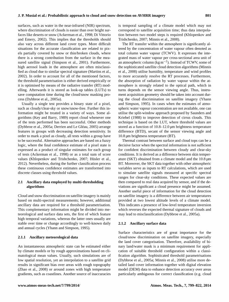
3.2.1 First enhanced spectral feature

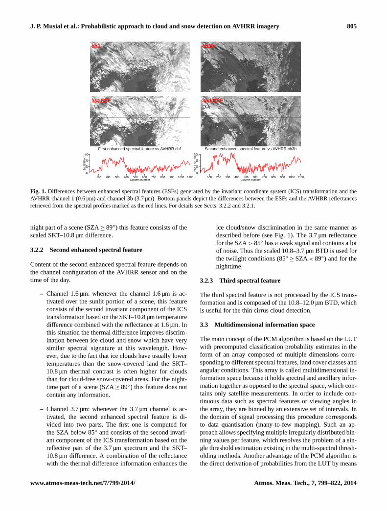
The first enhanced spectral feature consists of two compo-nents depending on the time of the day. For the sunlit por-tion of a scene limited by the SZA of 89◦ it is composedof the second invariant component of the ICS transforma-tion based on the SKT–10.8 µm temperature difference andon the reflectance at 0.6 µm over land and at 0.8 µm over wa-ter. This results in the enhanced spectral contrast because thincirrus or cold sub-pixel clouds modify thermal signal moreefficiently than the short-wave radiation (see Fig.1). For the

Atmos. Meas. Tech., 7, 799–822, 2014 www.atmos-meas-tech.net/7/799/2014/

J. P. Musial et al.: Probabilistic approach to cloud and snow detection on AVHRR imagery 805

ch1

1st ESF

1st E

SF

−ch

1

First enhanced spectral feature vs AVHRR ch1

Column number

010

2030

100 200 300 400 500 600 700 800 900 1000 1100

ch3b

2nd ESF

2nd

ES

F−

ch3b

Second enhanced spectral feature vs AVHRR ch3b

Column number

010

2030

100 200 300 400 500 600 700 800 900 1000 1100

Fig. 1. Differences between enhanced spectral features (ESFs) generated by the invariant coordinate system (ICS) transformation and theAVHRR channel 1 (0.6 µm) and channel 3b (3.7 µm). Bottom panels depict the differences between the ESFs and the AVHRR reflectancesretrieved from the spectral profiles marked as the red lines. For details see Sects.3.2.2and3.2.1.

night part of a scene (SZA≥ 89◦) this feature consists of thescaled SKT–10.8 µm difference.

3.2.2 Second enhanced spectral feature

Content of the second enhanced spectral feature depends onthe channel configuration of the AVHRR sensor and on thetime of the day.

– Channel 1.6 µm: whenever the channel 1.6 µm is ac-tivated over the sunlit portion of a scene, this featureconsists of the second invariant component of the ICStransformation based on the SKT–10.8 µm temperaturedifference combined with the reflectance at 1.6 µm. Inthis situation the thermal difference improves discrim-ination between ice cloud and snow which have verysimilar spectral signature at this wavelength. How-ever, due to the fact that ice clouds have usually lowertemperatures than the snow-covered land the SKT–10.8 µm thermal contrast is often higher for cloudsthan for cloud-free snow-covered areas. For the night-time part of a scene (SZA≥ 89◦) this feature does notcontain any information.

– Channel 3.7 µm: whenever the 3.7 µm channel is ac-tivated, the second enhanced spectral feature is di-vided into two parts. The first one is computed forthe SZA below 85◦ and consists of the second invari-ant component of the ICS transformation based on thereflective part of the 3.7 µm spectrum and the SKT–10.8 µm difference. A combination of the reflectancewith the thermal difference information enhances the

ice cloud/snow discrimination in the same manner asdescribed before (see Fig.1). The 3.7 µm reflectancefor the SZA> 85◦ has a weak signal and contains a lotof noise. Thus the scaled 10.8–3.7 µm BTD is used forthe twilight conditions (85◦ ≥ SZA< 89◦) and for thenighttime.

3.2.3 Third spectral feature

The third spectral feature is not processed by the ICS trans-formation and is composed of the 10.8–12.0 µm BTD, whichis useful for the thin cirrus cloud detection.

3.3 Multidimensional information space

The main concept of the PCM algorithm is based on the LUTwith precomputed classification probability estimates in theform of an array composed of multiple dimensions corre-sponding to different spectral features, land cover classes andangular conditions. This array is called multidimensional in-formation space because it holds spectral and ancillary infor-mation together as opposed to the spectral space, which con-tains only satellite measurements. In order to include con-tinuous data such as spectral features or viewing angles inthe array, they are binned by an extensive set of intervals. Inthe domain of signal processing this procedure correspondsto data quantisation (many-to-few mapping). Such an ap-proach allows specifying multiple irregularly distributed bin-ning values per feature, which resolves the problem of a sin-gle threshold estimation existing in the multi-spectral thresh-olding methods. Another advantage of the PCM algorithm isthe direct derivation of probabilities from the LUT by means

www.atmos-meas-tech.net/7/799/2014/ Atmos. Meas. Tech., 7, 799–822, 2014

806 J. P. Musial et al.: Probabilistic approach to cloud and snow detection on AVHRR imagery

of all available spectral and ancillary information. Thereforeall data are analysed at once in contrast to the decision-treealgorithms where features/tests are organised in a sequence.

The information space is composed of 8 dimensions:

– Time of the daydivided into day (SZA< 85◦), twilight(SZA≥ 85◦ and SZA< 89◦) and night (SZA≥ 89◦).

– First enhanced spectral featuredivided by the follow-ing binning values: 0, 0.025, 0.05, 0.075, 0.1, 0.125,0.15, 0.175, 0.2, 0.225, 0.25, 0.275, 0.30, 0.35, 0.40,0.45, 0.50, 0.60, 0.80 and 1.0.

– Second enhanced spectral feature:

– 1.6 µm channel activated: this feature is dividedby the following binning values: 0, 0.05, 0.075,0.1, 0.125, 0.15, 0.175, 0.2, 0.225, 0.25, 0.30,0.40, 0.50, 0.6 and 0.7.

– 3.7 µm channel activated: this feature is dividedby the following binning values: 0, 0.025, 0.05,0.075, 0.1, 0.125, 0.15, 0.175, 0.2, 0.225, 0.25,0.30, 0.40 and 0.50.

– Third spectral featuredivided by the following binningvalues:−0.8,−0.6,−0.4,−0.2, 0.0, 0.1, 0.4, 0.6, 0.8,1.0, 1.25, 1.5, 1.6, 1.8, 2.0, 2.5, 3.0 and 3.5.

– Texture feature, which is derived only over open watersby convolution of the 0.8 µm reflectance for the sunlitareas and the 10.8 µm BT during the nighttime with a3× 3 kernel (Eq.1). The convolution results are scaledto 0–1 range, where high values characterise pixels lo-cated at the cloud edges. This feature is divided by thefollowing binning values: 0.05, 0.1, 0.25, 0.5 and 1.

K =

−1 −1 −1−1 8 −1−1 −1 −1

(1)

– Sensor viewing sectors, which are derived by dividingthe satellite zenith angle with the following binningvalues: 0, 15, 30, 45, 55 and 70.

– Relative azimuth sectors, which are derived by di-viding the relative azimuth (RAZ) angle, defined asa difference between Sun and sensor azimuth angles(180◦ = forward scattering), with the following binningvalues: 0, 45, 90, 135 and 180.

– Land cover/usedeveloped within the scope ofthe Global Land Cover 2000 (GLC2000) project(Bartholomé and Belward, 2005). There are three ad-ditional surface categories which are derived internallyby the PCM algorithm: coastline water defined as a8 km buffer zone from the shore including inland wa-ters, Sun glint over water and Sun glint over desert,

which are discriminated by the simple Sun–sensorangular dependency described byAckerman et al.(1998). All these areas feature significantly higherreflectances due to specific angular conditions (Sunglint); higher concentration of non-maritime aerosols(Wang and Shi, 2006), sediments or algae (Wang andShi, 2005) and shoreline variation induced naturally bytides or artificially by satellite geolocation problems.

The positions of values within the information space de-pend on diurnal and annual cycles. The first one is driven bythe illumination conditions and alters mainly the reflectancedue to the bidirectional effects. Therefore separate informa-tion spaces were developed for different satellite overpasstimes. For morning satellites with the 1.6 µm channel acti-vated, acquisition time was divided into two ranges: 00:00–12:00 and 13:00–00:00 UTC. For the satellites with the3.7 µm channel activated the division was set to 07:00–10:00,11:00–14:00, 15:00–18:00, and 19:00–06:00 UTC. The an-nual cycle is related to changes in albedo and surface emis-sivity properties induced by vegetation development and soilmoisture variations. Thus the information spaces were fur-ther divided between different seasons: winter (November–January), spring (February–April), summer (May–July), andautumn (August–October). Each possible daytime–seasoncombination was stored separately for the 1.6 and 3.7 µmchannel configurations, which results in 48 LUTs.

P ∈

0 ≤ P ≤ 100 probability of 0–100 % betweenclear-sky and snow conditions

100 ≤ P ≤ 200 probability of 0–100 % betweensnow and cloudy conditions

200 ≤ P ≤ 300 probability of 0–100 % betweencloudy and clear-sky conditions

(2)

3.4 Methodology of classification

In order to discriminate snow, clear-sky and cloudy pixelson a satellite image with the PCM algorithm, the informa-tion space has to be filled with classification probability es-timates. This process is divided into 2 steps. First, a tempo-rary information space is created which contains one moredimension where the categories clear-sky, cloudy and snoworiginating from the training data set are stored. Second, thefrequencies of occurrence of those classes within each binare transformed into the probability estimates. Developmentof the PCM method consists of the following steps:

1. Composition of training data set, which involvescollocation of the AVHRR measurements with thesnow/clear-sky/cloudy classification which may orig-inate from ground data, supplementary satellite datasource (e.g. CALIPSO and MODIS products) or fromresults of another classification algorithm applied tothe AVHRR data. Nevertheless, the data quantityshould be large enough to sufficiently sample the mul-tidimensional array with information acquired under a

Atmos. Meas. Tech., 7, 799–822, 2014 www.atmos-meas-tech.net/7/799/2014/

J. P. Musial et al.: Probabilistic approach to cloud and snow detection on AVHRR imagery 807

wide range of environmental conditions. In this studythe training data set was composed of the PPS version2012 cloud masks (Dybbroe et al., 2005a) retrievedfrom AVHRR data and merged with the MOD10A1daily snow masks (Hall et al., 2002) based on MODISdata. Those algorithms were selected due to their highclassification accuracy (Dybbroe et al., 2005b; Halland Riggs, 2007), as well as the data (MOD10A1)and source code (PPS) availability. It has to be em-phasised that the mean PCM classification accuracycannot exceed the one associated with the training dataset. To improve the quality of the training data set,it was first visually inspected and low-quality sceneswere removed. Then significant misclassifications oc-curring in the remaining images were edited and cor-rected by an analyst. This procedure was applied tothe extensive data set (∼ 2400 scenes) acquired overEurope between 2009 and 2011 by different AVHRRsensors mounted aboard NOAA satellites denoted withnumbers 16, 17, 18 and 19.

2. Formation of temporary information spaces, which in-volves computation of all spectral and textural fea-tures for the selected AVHRR training images. Further,the frequencies of occurrence of clear-sky, snow andcloudy classes originating from the training data foreach combination of dimensions (i.e. features, angu-lar and ancillary data) are inserted into the informationspace. Therefore, a single value within the temporaryinformation space corresponds to numerical count ofall pixels embedded into a nine-dimensional bin com-posed of the following elements: time of the day, threespectral features, texture feature, viewing and azimuthsectors, land cover, and PPS/MOD10A classification.In other words this array might be treated as a nine-dimensional histogram. This procedure was repeated48 times for each information space characterised bythe different channel configuration (1.6/3.7 µm), acqui-sition hour and season.

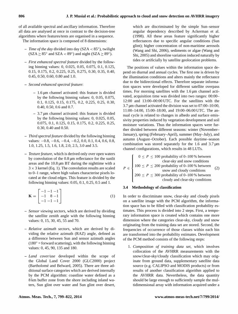
3. Derivation of classification probability, which is basedon numerical counts from the temporary informationspaces, which are first rearranged in descending or-der for every multidimensional bin. Further, the prob-ability is computed as a simple ratio between countsof the most frequent classification category within abin and the total number of counts in this bin. Theretrieved value is described as a classification prob-ability between the two most frequent classes withinthe bin. Similar analysis in a two-dimensional space ispresented in Fig.2. The PCM classification probabil-ity estimates are related to a combination of the fol-lowing categories: snow-free/snow, clear-sky/cloudy,snow/cloudy. For the sake of visualisation obtainedvalues are recoded according to Eq. (2). For bins which

Fig. 2. Schematic graph presenting the concept of probabilityderivation in the PCM algorithm based on the two-dimensionalspectral space composed of the reflectances at 0.6 and 1.6 µm. Inthe equationP denotes probability and numbers denote the countsof cloudy, clear and snow pixels within a bin. The samples were de-rived from the PPS and MOD10A1 classifications of the NOAA17satellite scene acquired over the Alps on 1 January 2008.

were not filled by the training data set probability es-timates are retrieved by the nearest-neighbour interpo-lation of existing values within the array. At the laststage, all information spaces containing probability es-timates are compressed and stored in the NetCDF4 for-mat as the LUTs.

4. Classification of a satellite imageis a procedure verysimilar to the construction of temporary informationspaces because it requires preparation of the samespectral and ancillary data (binned values of spectralfeatures, angles, etc.). However, this information isfurthermore directly used to retrieve probability esti-mates from a LUT. The bottleneck of this process isrelated to localisation of all input data associated witha large satellite scene within a LUT, which itself hasmore than 60 million values. This issue is resolved bythe fast approximate near-neighbour (ANN) searchingmethod (Arya et al., 1998) which is performed for eachdimension separately.

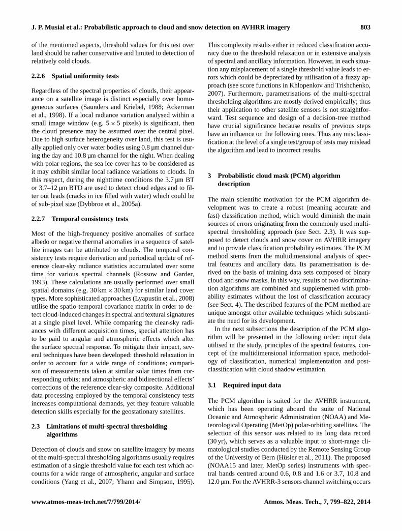
3.5 PCM numerical implementation

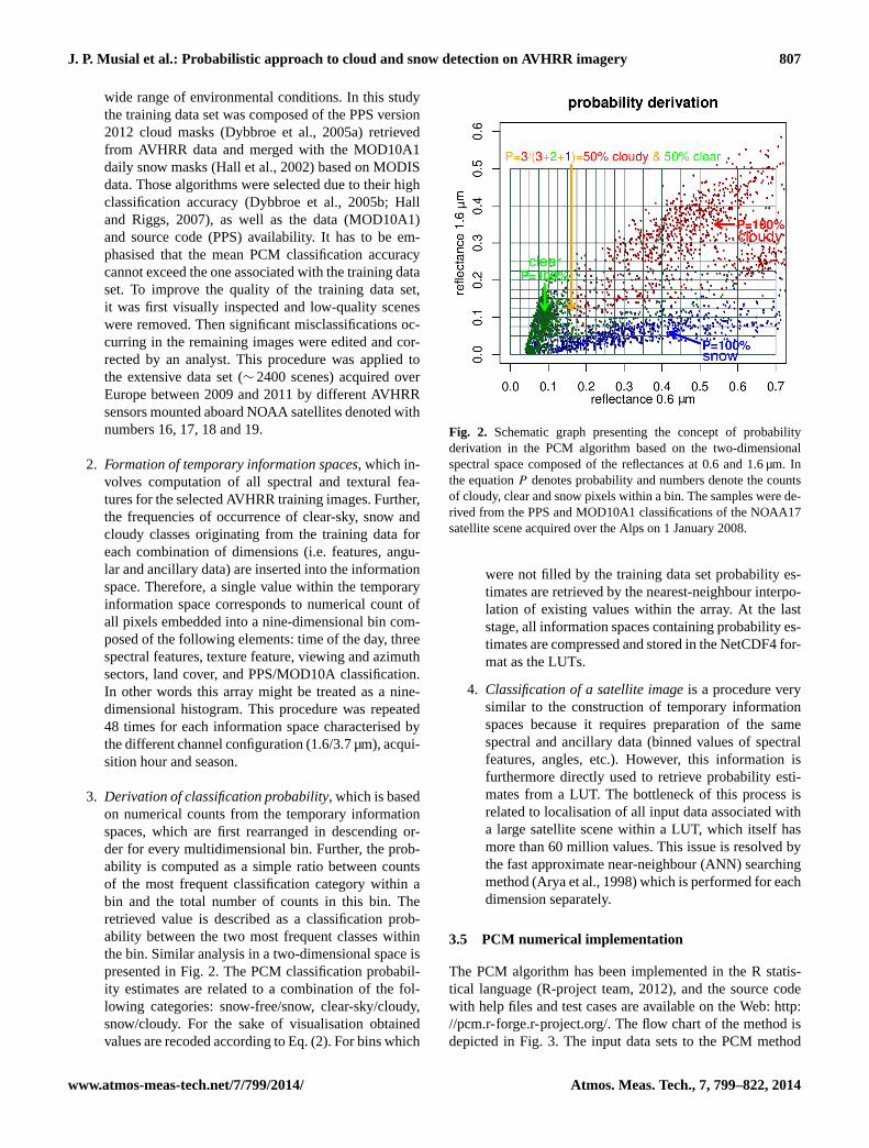
The PCM algorithm has been implemented in the R statis-tical language (R-project team, 2012), and the source codewith help files and test cases are available on the Web:http://pcm.r-forge.r-project.org/. The flow chart of the method isdepicted in Fig.3. The input data sets to the PCM method

www.atmos-meas-tech.net/7/799/2014/ Atmos. Meas. Tech., 7, 799–822, 2014

808 J. P. Musial et al.: Probabilistic approach to cloud and snow detection on AVHRR imagery

Fig. 3.Flow chart of the PCM algorithm. For details see Sect.3.5.

require few pre-processing steps, which consist of discrimi-nation of shallow water defined as a 8 km buffer zone froma shore, Earth distance correction of reflectances, and up-scaling of the SKT estimates. The last process involves bi-linear and temporal interpolation of two SKT estimates clos-est to the satellite overpass time. They are usually of muchcoarser spatial resolution than the AVHRR grid and corre-spond to certain hours. The upscaled data do not resolve wellthe temperature variation in rough topography terrains suchas high mountains. To account for this effect, a constant tem-perature correction is derived by multiplying the lapse rateof 0.6 K 100 m−1 with the altitude difference between the1 km× 1 km DEM provided by the USGS and the bi-linearlyupscaled 0.2◦ × 0.2◦ DEM (geopotential at surface) originat-ing from the ECMWF model. This correction is added to thefinal SKT estimates.

At the first stage of the PCM algorithm the required data– AVHRR reflectances and brightness temperatures, viewzenith angle (VZA), SZA, RAZ, land cover, upscaled SKTand the DEM – are ingested, and no-data values are removed.Further, several processes are performed:

α

αβ

βγ

δ

βγ

δ

L

L

h

Lh

Y

X

XY

sun zenith anglesun elevation anglesun azimuth anglereduced azimuth anglecloud shadow lengthcloud top heightdisplacement along x axisdisplacement along y axis

cloud

cloud

pixelshadow

pixel

Fig. 4.Derivation of cloud shadow. For details see Sect.3.6.

– Division between day, twilight and night (seeSect.3.3).

– Derivation of reflectance from the 3.7 µm BT.

– Identification of Sun glint areas (afterAckerman et al.,1998) over water and desert which are incorporatedinto the land cover data.

– Kernel convolution and derivation of the texture fea-ture from the 0.6 and 10.8 µm channels.

Further reflectances and the thermal difference betweenSKT and the 10.8 µm BT are fetched into the ICS trans-formation separately suited for the 1.6/3.7 µm channels. Forthe daytime data its results consist of two enhanced spectralfeatures, where the first one together with the 10.8–12.0 µmBTD are the same for both channel configurations. For thenighttime the first two features contain scaled SKT–10.8 µmand 3.7–10.8 µm BTD respectively. Such processed spectralinformation, together with the texture feature, acquisition an-gles and expanded land cover data, are located within the bin-ning values (see Sect.3.3) by means of the ANN procedure(Arya et al., 1998). This leads to determination of indicesalong each of the eight dimensions of the information spacewhich are merged into two separate tables depending on the3a/3b channel availability. Finally, the index tables are usedto retrieve classification probability estimates from the LUTsfor every pixel in a satellite scene.

SAZred =

SAZ ∈ 0 ≤ SAZ ≤ 90; Xscale= −1; Yscale= −1SAZ − 90 ∈ 90 < SAZ ≤ 180; Xscale= −1; Yscale= 1SAZ − 180∈ 180 < SAZ ≤ 270; Xscale= 1; Yscale= 1SAZ − 270∈ 270 < SAZ ≤ 360; Xscale= 1; Yscale= −1

(3)

x2 = L × sin(SAZred) × Xscale+ x1y2 = L × cos(SAZred) × Yscale+ y1

(4)

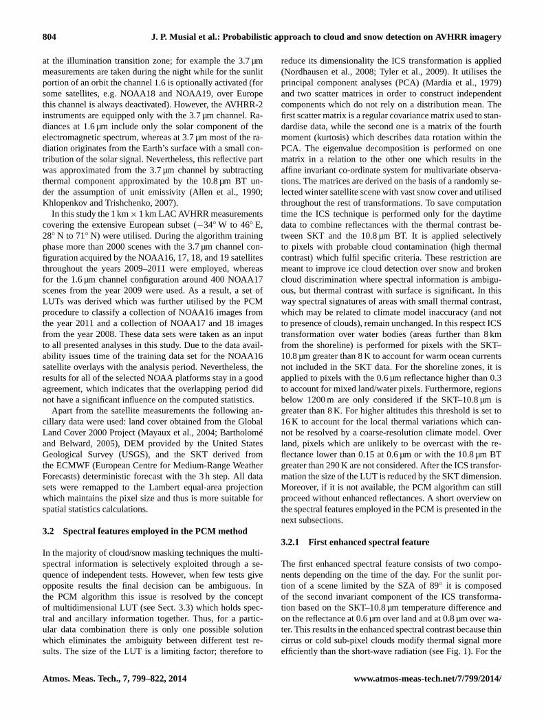
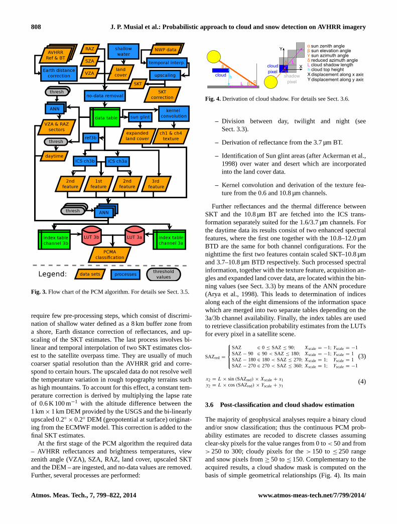
3.6 Post-classification and cloud shadow estimation

The majority of geophysical analyses require a binary cloudand/or snow classification; thus the continuous PCM prob-ability estimates are recoded to discrete classes assumingclear-sky pixels for the value ranges from 0 to< 50 and from> 250 to 300; cloudy pixels for the> 150 to ≤ 250 rangeand snow pixels from≥ 50 to≤ 150. Complementary to theacquired results, a cloud shadow mask is computed on thebasis of simple geometrical relationships (Fig.4). Its main

Atmos. Meas. Tech., 7, 799–822, 2014 www.atmos-meas-tech.net/7/799/2014/

J. P. Musial et al.: Probabilistic approach to cloud and snow detection on AVHRR imagery 809

a) b) c)

Fig. 5.PCM classification example of the NOAA17 scene acquired over the Alps on 1 January 2008 at 10:00 UTC.(a) False-colour composite(R = 1.6 µm,G = 0.8 µm,B = 0.6 µm),(b) probabilistic cloud and snow mask,(c) binary cloud/cloud shadow/snow/land-water mask withclasses described in Sect.3.6. In (b) and (c) grey colour depicts clouds, green depicts snow-free areas, blue depicts water and light bluedepicts snow.

aim is to provide a rough approximation of a cloud shadowlocation which could be useful for derivation of clear-skycomposites. However, if more accurate cloud shadow maskis required, please refer to the study ofSimpson and Stitt(1998). In the PCM cloud shadow derivation consists of sev-eral steps. First, a rough approximation of cloud heighth isestimated from the SKT–10.8 µm thermal contrast assumingthe constant temperature lapse rate of 0.6 K 100 m−1. Sec-ond, the acquired altitude values are processed by the maxi-mum value filter with a 5× 5 window to enhance reliabilityof the estimates at cloud edges, where the thermal contrast issmaller due to fractional cloud cover. Subsequent computa-tions are performed only for pixels located at cloud edges andinitially involve calculation of shadow lengthL, expressedas cloud height divided by the tangent of Sun elevation angle(90◦

−SZA). Next, the Sun Azimuth angle (SAZ) is reducedto 0–90◦ range (SAZred), and theXscaleandYscaleare derivedaccording to the convention described by the Eq. (3). Finally,the shadow end (x2, y2) is estimated from the coordinatesof the centre of a cloud edge pixel (x1, y1) and displacementvectors alongx andy axis, computed as a ratio of the shadowlength and sine and cosine of the SAZred respectively (Eq.4).

The acquired cloud shadow mask is incorporated togetherwith the land cover data into the PCM binary output to com-pose a discrete classification which consists of the followingcategories: no data, clear-sky water, clear-sky land, clear-skysnow, pixel adjacent to cloud over water, pixel adjacent tocloud over land, pixel adjacent to cloud over snow, cloudshadow over water, cloud shadow over land, cloud shadowover snow, and cloud. An example of the PCM output (Fig.5)presents the NOAA17 AVHRR scene acquired over the Alpson 1 January 2008 together with the probability estimates andthe discrete classification mask.

3.7 Limitations of the PCM algorithm

Apart from the advantages of the PCM method – such as de-termination of classification probability for clear-sky, snowand cloudy conditions, and unsupervised algorithm trainingphase – there are some methodological limitations. Althoughthe algorithm provides a great flexibility over other classi-fication methods in terms of selection of numerous binningvalues, their choice is still a matter of subjective decision.Nevertheless, it is possible to determine an arbitrary numberof regularly distributed binning values for each feature, andstill the algorithm will exhibit considerable detection skills.The approach applied in this study assumes higher densityof bins around value ranges associated with uncertain pixels(e.g. low reflectance values related to broken/cirrus clouds).Furthermore, the number of intervals modifies the probabil-ity values, as wider bins within the information space aremore likely to contain a mixture of classes in comparison tosmaller bins. Thus, a high density of binning values assuresbetter classification accuracy at the price of bigger LUT size,which itself is a limiting factor.

The quality of the PCM results mostly depends on theaccuracy of the clear-sky/snow/cloud mask used during thealgorithm training step. Moreover, the quantity of trainingdata should be large enough to sufficiently sample the multi-dimensional array with information acquired under a widerange of environmental conditions. Although in this studya broad set of ecosystems was considered (from deserts totundra and perennial ice), the performance of the methodover other regions than Europe is still to be determined, aswell as the applicability to the older AVHRR sensor (prior toNOAA16).

www.atmos-meas-tech.net/7/799/2014/ Atmos. Meas. Tech., 7, 799–822, 2014

810 J. P. Musial et al.: Probabilistic approach to cloud and snow detection on AVHRR imagery

●●●

●

●●

●●

●

●

●

●●

● ●●● ●

●

●●●

●

●● ●

●

●●●●

●●●●●

●● ●

●

●●

●●

●

●

●●●

●●● ●

●

●

●

●

●●

●● ●●●●

●●●●

●●

●

● ●●●

●

●

● ●

●

● ●

●

●●

●●

●●

●●

●

● ●

●

●●

●

●

●●

●

●●

●

● ●

●

●

●

●

●

●●

● ●●

●●●

●

●

●●

●

●●

●

●

●

●

● ●●●●

●●●

●●

●●

●●

● ●●

●

●

● ●●● ●●

● ●●

●●

●

●●●

●●● ●●

●

●

● ●

●

●●

●

●

●

●

●●

●●

●●●

●●●● ●

●

●

●

●

●●

●

●

●

●

●

●

●

●●

●

●●

●

●●

●●

●

●●●

●●

●

●

●●●

●

●●●●●

●●

●●●

●

●

●

●

●

●

●

●● ●

●

●

●

●●●

●

● ●● ●

●

●

●

●●

●

●●●

●●

●●

●

●

●

●

● ●

●●

●●

●●

●

●●

●●

●

●

●

●

●

●

●

●

●

●●

●●

●

●●

●

●

●

●

●●●

●

●● ●●

●●

●●●

●

●●●

●

●●

●●

●

●

●

●

●

●

●

●●

●

● ●

●

●●

●

●

●●

●

●

●●

●●

●●●

●●●

●

●

●

●

●●

●●●●

●

●●

●

●●

●

●

●

●

●

●

●

●●

●

●

●

●●

●

●

●●

●

●

●●

●

●

●●

●●

●

●

●

●

●●

●

●●●

●

●

●

●

●●●

●●

●

●●

●

●

●●

●

●

●●

●●●

●

●●

●

●

●

●

●●●

●

●

●●●

●

●●

●●

●●

●

●●

●

●

●

●

●

●●

●

●●

●

●●

●●●

●●

●●

●

●●●●

●●●

●

●

●

●

●

●

●

●

●

●

●

●

●

●●

●

●

●

●

●

●

●

●

●

●

●●

●

●●●

●

●●

●●●

●

●●

●

●

●●

●

●

●

●

●

●●

●

●●

●

●

●

●

●●

●

●

●●

●

●●●

●●●

●

●

●

●

●

●

●

●

●●

●

●

● ●

●

●

●●

●●

●

●

●

●

●

●

●

●

●

●●

●

●

●●

●

●●

●

●

●

●

●

●

●

●

●

●

●

●

●

●● ●

●

●

●

●

●●

●

●●●

●

●

●

●

●

●

●

●

●

●●●

●

●●●●

●

●

●●

●●●

●

●●

●

●

●

●

●

●

●●

●

●

●●

●

●

●

●

●

●

●

●

●●●●

●

●

●

●

●

●

●

●

●●●

●●●

●

●●

●

●

●●

●

●●

●

●

●●●●●

●●

●●

●

●●●

●

●●

●

●●●●

●

●

●●

●●●

●

●●

●●● ●

●●●

●

●●●

●●●●

● ●●●●●●●

●● ●●

●

●●

●

●

●●

●

●●

●●●

●●●

●

●●●

●

●

●

●

●●

●

●●

●

●

●

●

●

●

● ● ●●●

●

●

●

●●

●

●●

●

●●●

●

●

●●

●●●●●

●

●●

●

●

●

●

● ●

●

●

●

●

●

●●

● ●●●

●

●

●●

●

● ●●●

●

●●

●●

●●●

●

●●

●●

●●

●

●

●●

●

●

●

● ●

●

●

●

●●

● ●●

●

●

●

●●

● ●●●●

●

●

●●

●●●

●

●

●●

●●

●

●

●

●

●●

●

●

●

●●●●

●●●●

●

●

●

●

●

●

●

●

●

●

● ●●●●

●

●

●

●

●

●●●●

●

20 40 60 80 100

2040

6080

100

PCM [%]

PP

S [%

]

NOAA16

a)

PCM−PPSmedian = 0.32mean = 0.87stdev = 3.56R2 = 0.93 ●

●

●

●

●

●

●●●

●

●

●●●

●

●●●●

●

●●

●●

●

●●

●●●

●

●●

●●●●●

●●

●

●●●

●●●

●

●●

●

●

●

●●

●

●

●●●●●

●●

●

● ●

●

●●

●

●●

●

●●

●

●

●●

●

●

●

●●●●

●

●●

●●

●

●

●

●

●●●

●

●

●

●

●

●●●

●

●

●●

●

●

●

●

●●●

●●

●

●●

●

●●

●●●

●

●

●

●

●

●

●

●●●

●●●

●

●

●

●

●

●

●●

●●

●●

●●

●

●

●

●

●●●

●●

●

●

●

●

●

●

● ●●●●

●●●●●

●

●

●

●●

●

●

●●●

●

●

●

●

●●

●

●

●

●

●

●●

●●●●

●

●●

●●

●

●

●

●●●

●

●

●

●●

●

●

●●

●●

●

●

●

●

●

●

●●

●●

●

●●

●

●●●●●●

●

●

●

●●

●●●

●

●

●

●

●

●●

●

●

●

●

●●

●●

●

●●

●●

●

●

●

●●

●

●

●

●

●

● ●

●

●

●

●

●●

●

●●●

●●

●

●

●

●

●●

●

●

●●

●●

●

●

●

●

●●●

●●●

●●

●●

●

●

●

●

●●

●

●

●●

●

●

●

●

●

●

●

●

●●

●●●

●

●

●

●

●

●

●

●●

●

●

●●

●

●

●

●

●●

●

●

●

●

●●

●

●●

●

●

●

●

●

●

●

●

●

●

●●

●

●

●●

●

●

●●

●●

●

●

●

●●

●

●

●

●

●

●

●

●

●

●

●

●

●

●

●

● ●●

●

●

●

●

●

●

●

●●

●●●

●

●

●

●

●●

●

●●

●

●

●

●

●

●

●

●

●●

●

●

●●

●

●

●

●●

●

●

●●

●

●

●

●

●

●●

●●

●●●

●

●●

●

●

●

●

●●

●

●●

●

●

●

●

●●

●

●

●

●

●

●

●

●●

●

●

●

●

●

●

●

●

●

●

●●●●

●

●

●●

●●

●●

●

●

●

●

●●

●●●

●

●

●

●

●

●

●

●

●

●

●

●●

●●

●

●

●

●

●

●

●

●

●

●

●●●

●

●

●

●

●

●

●

●

●●

●●

●

●●●

●●

●

●●●●

●

●

●

●

●

●

●

●●

●●

●●●

●

●

●

●

●

●●

●

●●

●

●

●

●

●

●

●

●

●

●

●●

●●●

●

●

●

●

●

●

●

●●●●●●

●

●

●●

●

●●

●

●

●

●

●

●

●●

●●

●

●

●●

●

●

●● ●

●

●●

●

●

●

●

●●

●

●

●

●

●●

●

●

●●

●

●

●

●●● ●●

●●

●

●

●

●

●●

●

●

●

●

●

●

●●

●

●

●

●

●

●●●

●●

●●

●●

●

●

●

●

●●

●

●

●

●●

●

●

●

●

●

●

●

●

●

●●

●

●

●

●

●

●

●●

●

●

●

●

●●

●

●

●

●

●

●

●

●

●●●

●

●

●●

●

●●

●●

●●

●

●

●●

●

●

●

●

●●

●●●

●

●

●

●

●

●●

●

●

●●

●

●

●●

●●●●

●●●

●●

●

●

●

●

●●

●

●●●●●

●●●

●●●

●

●●

●

●●

●

●

●●●

●●●●●

●

●

●●

●

●●

●●●

●

●●

●

●●

●

●

●●

●●

●

● ●

●●●

●

●

●●●

●

●●

●

●

●

●●

●●

●

●●●

●

●●

● ●● ●●

●●

●

●

●

●

●

●●

●●

●

●

●●● ●

●

●●

●

●

●●

● ●

●

●

●

●

●

●

●

●●

●

● ●

●

●

●●●●

●●

●●●●

●●●

●

●●

● ●

●●●

●

●

20 40 60 80 100

2040

6080

100

PCM [%]

PP

S [%

]

NOAA17

b)

Total cloud cover PCM vs PPS

PCM−PPSmedian = −0.49mean = −0.46stdev = 3.48

R2 = 0.94●●

●

●

●●

●●

●●

●

●

●

●

●

●

●

●

●

●●

●●●

●●

●

●●

●●●

●●

●●

●●

●

●

●

●●

●

●

●

●

●

●●●

●

●●

●

●●

●●●

●●

●

●

●

●

●

●

●

●

●

●

●

●

●●

●

●

●

●●

●●

●

●●

●

●●

●●

●●

●

●

●

●

●

●●

●

●

●

●

●

●●

●●

●●

●●

●

●●

●

●

●

●

● ●

●

●●

●

●

●

●●

●

●●

●

●

●

●

●

●

●●

●

●

●

●

●

●●

●●

●●●

●

●

●

●●

●

●

●

●●

●

●●

●

●

●

●

●

●

●

●

●

●

●

●

●●

●

●●

●

●

●●

●

●

●

●

●●

●

●

●

●●

●●●

●●

●

●

●

●●

●

●●

●

●

●●●

●●

●

●

●

●

●

●

●

●

●●

●

●

●

●●

●

●●

●

●

●

●●

●

●

●

●

●

●

●

●●

●

●

●

●

●

●●

●

●

●

●

●

●

●

●

●●

●

●●

●

●

●●

●

●

●

●

●●

●

●●

●

●●

●

●

●

●

●

●

●

●

●●

●

●

●

●

●●

●

●●

●

●

●●

●

●

●

●

●●

●

●●

●

●

●

●

●

●

●

●

●

●

●

●

●

●

●

●

●

●●

●

●

●

●

●●

●

●●

●

●

●

●●

●

●

●

●

●

●

●

●●

●

●●

●

●

●

●

●●

●

●

●

●

●●

●

●

●

●

●

●

●

●

●

●

●

●

●

●

●

●

●

●●

●

●●

●

●●

●

●●

●

●

●

●

●●

●

●

●

●

●

●

●●

●

●

●●

●

●

●

●

●

●

●

●

●

●

●

●

●

●

●

●

●

●

●

●

●

●

●

●

●●

●

●●

●

●●

●

●●

●

●

●

●

●

●

●

●

●

●

●

●●

●

●●

●

●●

●

●

●

●

●

●●

●

●

●

●●

●

●

●

●

●●

●

●

●

●

●

●

●

●●

●●●

●

●

●

●

●

●

●

●●

●

●

●

●

●

●●

●

●●

●●●

●●

●

●●

●

●

●

●●

●

●

●

●

●

●

●

●

●

●

●

●

●

●●

●

●

●

●

●

●●

●

●●

●

●●

●

● ●

●

●

●

●●

●

●●

●

●

●●

●

●

●

●

●●

●

●●

●

●●

●

●●

●

●

●

●

●

●

●●

●

●

●

●

●

●

●

●

●

●

●

●

●

●

●

●

●

●●

●

●

●

●

●

●

●

●●

●

●●

●

●

●●

●

●

●

●

●

●

●

●

●

●

●

●

●

●

●

●

●

●

●●

●

●●●

●

●

●

●●

● ●

●

●

●

●●

●

●

●

● ●

●

●●

●

●●

●●

●

●

●

●

●●

●

●

●

●

●

●●

●

●

●

●

●

●

●

●

●

●

●

●

●

●

●●●

●

●●

●

●●

●

●

●

●

●

●

●●

●

●● ●

●

●

●

●

●

●

●

●

●

●●

●

●●

●●

●

●

●

●

●

●

●

●

●

●●

●

●●

●

●

●

●

●●

●●

●

●

●●

●

●

●●

●

●

●●

●

●

●

●●●

●

● ●●

●

●

●

●

●

●

●

●

●

● ●●

●●

●●

●

●●

●

●●

●

●●

●●

●

●

●●

●

● ●●

●

●

●

●

●

●

●●

●

●●

●

●

●

●

●

●●

● ●

●

●

●●●

●●

●

●●

●

●●●

●

●

●●

●

●

●

●

●●

●●●

●●

●●

●●

●

●●

●●●

●

●

●●

●●

●●●

●●

● ●●

●

●

●●

●

●●

●

●

●●●●

●● ●

●●●

●● ●

●●

●

●●

●

●●●

●●●●

● ●●

● ●●

●

●●

●●

●

●●

●

●

●

●

●

●●

●

●●●

●

●

20 40 60 80 100

2040

6080

100

PCM [%]

PP

S [%

]

NOAA18

c)

PCM−PPSmedian = −0.01mean = −0.39stdev = 2.57R2 = 0.97

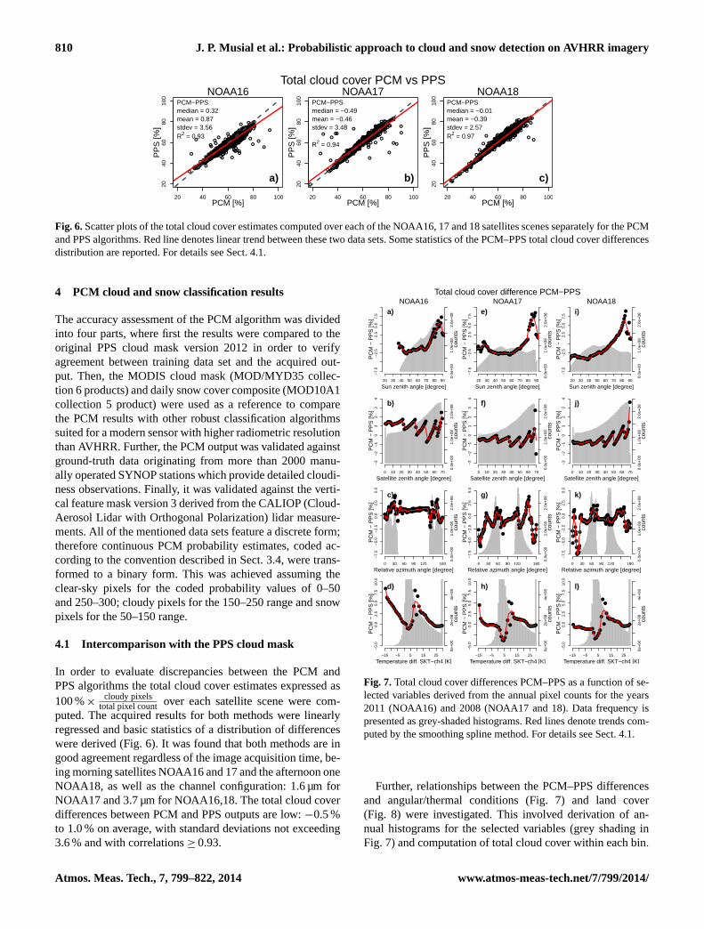
Fig. 6.Scatter plots of the total cloud cover estimates computed over each of the NOAA16, 17 and 18 satellites scenes separately for the PCMand PPS algorithms. Red line denotes linear trend between these two data sets. Some statistics of the PCM–PPS total cloud cover differencesdistribution are reported. For details see Sect.4.1.

4 PCM cloud and snow classification results

The accuracy assessment of the PCM algorithm was dividedinto four parts, where first the results were compared to theoriginal PPS cloud mask version 2012 in order to verifyagreement between training data set and the acquired out-put. Then, the MODIS cloud mask (MOD/MYD35 collec-tion 6 products) and daily snow cover composite (MOD10A1collection 5 product) were used as a reference to comparethe PCM results with other robust classification algorithmssuited for a modern sensor with higher radiometric resolutionthan AVHRR. Further, the PCM output was validated againstground-truth data originating from more than 2000 manu-ally operated SYNOP stations which provide detailed cloudi-ness observations. Finally, it was validated against the verti-cal feature mask version 3 derived from the CALIOP (Cloud-Aerosol Lidar with Orthogonal Polarization) lidar measure-ments. All of the mentioned data sets feature a discrete form;therefore continuous PCM probability estimates, coded ac-cording to the convention described in Sect.3.4, were trans-formed to a binary form. This was achieved assuming theclear-sky pixels for the coded probability values of 0–50and 250–300; cloudy pixels for the 150–250 range and snowpixels for the 50–150 range.

4.1 Intercomparison with the PPS cloud mask

In order to evaluate discrepancies between the PCM andPPS algorithms the total cloud cover estimates expressed as100 %×

cloudy pixelstotal pixel count over each satellite scene were com-

puted. The acquired results for both methods were linearlyregressed and basic statistics of a distribution of differenceswere derived (Fig.6). It was found that both methods are ingood agreement regardless of the image acquisition time, be-ing morning satellites NOAA16 and 17 and the afternoon oneNOAA18, as well as the channel configuration: 1.6 µm forNOAA17 and 3.7 µm for NOAA16,18. The total cloud coverdifferences between PCM and PPS outputs are low:−0.5 %to 1.0 % on average, with standard deviations not exceeding3.6 % and with correlations≥ 0.93.

0.0e

+00

1.0e

+08

2.0e

+08

20 30 40 50 60 70 80 90

a)

coun

ts

Sun zenith angle [degree]

PC

M −

PP

S [%

]

NOAA16

●

●●●●●

●●●●●

●●●●●●●

●●●●●●●●●●

●●●

●●●●●

●●●●●●●

●

●

●

●

●

●

●

●●

●

●●●●●●

●●●●●●●●●●●●●●●●●●

●●●●●●●●●●●●●●●●●●●

●●

●●●

−7.

5−

2.5

2.5

5.0

7.5

0.0e

+00

1.0e

+08

2.0e

+08

0 10 20 30 40 50 60 70

b)

coun

ts

Satellite zenith angle [degree]

PC

M −

PP

S [%

]

●●●●●●●●

●●●●●●●●

●●●●●

●

●

●●●●●

●●●●

●●●●

●

●

●●●●

●●●●●●●●

●●●●●●●●●●●

●

●

●

●

●

●

●

●

●

−3

−2

−1

01

23

4

0.0e

+00

1.0e

+08

2.0e

+08

0 30 60 90 120 180

c)

coun

ts

Relative azimuth angle [degree]

PC

M −

PP

S [%

]

●

●●●●●●●●●●●

●●●●●●●●●

●●●●●●●●

●●

●●

●

●

●●

●●

●

●●

●●●●●

●●

●

●●●●●●●●●●●●●●●●●●●●●●●●●●●●●●●●●●●

●●●●●●●●●●●●●●●●●●●●●●●●●●●●●●●●●●●●●●●●●●●●

●●●●●●●●●●●

●

●●

●

●●

●

●●

●●

●●●

●

●

●●●

●

●●●●

●

●

●●

●●●●●●●●●●●●●

−7.

5−

5.0

−2.

50.

02.

55.

0

0e+

002e

+08

4e+

08

−15 −5 5 15 25

d)

coun

ts

Temperature diff. SKT−ch4 [K]

PC

M −

PP

S [%

]

●

●●●●●●●●●●●●●●●

●

●●●●

●

●

●

●

●

●

●●●

●●●●●●●

●●●●●●●●

−5.

00.

02.

55.

07.

510

.0

0.0e

+00

1.0e

+08

2.0e

+08

20 30 40 50 60 70 80 90

e)

coun

ts

Sun zenith angle [degree]

PC

M −

PP

S [%

]

NOAA17Total cloud cover difference PCM−PPS

●

●

●

●

●●●●●●

●●●

●●●●●●

●●●●●●●●●●●●●●●●●●●●●●●●●●●●

●●●●●

●●●●●●●

●●●●

●●●●

●

●

●

●

●

●

●

●●

●

●●●●●●

●●●●●●●

●●●●●●●●●●●●●●●●●●

●●●●●●●

●●●●●

●●●●●●●●●●●●●●●●●●●●●●●

●

●

●

●

●

−7.

5−

2.5

2.5

5.0

7.5

0.0e

+00

1.0e

+08

2.0e

+08

0 10 20 30 40 50 60 70

f)

coun

ts

Satellite zenith angle [degree]

PC

M −

PP

S [%

]

●●●●●●●●●●●●●●

●●●●●

●●●

●

●●●●●●●

●●●●●●●

●

●●●●●

●●●●

●●●

●●●●

●●●●

●●●●

●

●●●●

●

●

●

−3

−2

−1

01

23

4

0.0e

+00

1.0e

+08

2.0e

+08

0 30 60 90 120 180

g)

coun

ts

Relative azimuth angle [degree]

PC

M −

PP

S [%

]

●

●

●●

●●●

●●●●●●●

●●●●●

●●●●

●

●●●●●●●●●●●

●●●●●●●●●●●

●●●●●●

●●●●●

●●

●●●●●

●●

●

●●

●

●●

●●

●

●

●

●●●●●●●●●●●●●●●●●●●●●●●●●●●●●●

●●●●●

●●●●

●●●●●

●●

●●

●

●

●●●●●●●●●●●●●●●●●●●●●●

●●●●●●●●

●

●

●●●●●●●●

●

●

●●●●●●●

●●●

●

●

−7.

5−

5.0

−2.

50.

02.

55.

0

0e+

002e

+08

4e+

08

−15 −5 5 15 25

h)

coun

ts

Temperature diff. SKT−ch4 [K]

PC

M −

PP

S [%

]

●

●●●●●●●●●●●●●●●

●

●

●●●

●

●

●

●

●

●

●●●●●●●●●●

●●●●●●●●

−5.

00.

02.

55.

07.

510

.0

0.0e

+00

1.0e

+08

2.0e

+08

20 30 40 50 60 70 80 90

i)

coun

ts

Sun zenith angle [degree]

PC

M −

PP

S [%

]

NOAA18

●

●

●

●

●●

●

●●●●

●●●●●●●●●●●●●●●●●●●●●●●●●●●

●●●●●

●●●●●●●

●●●●●

●●●●●

●●●●

●●●●

●●●●●●

●

●

●

●●●

●

●●●●●●

●●●●●●●●●●●●●●●●●●

−7.

5−

2.5

2.5

5.0

7.5

0.0e

+00

1.0e

+08

2.0e

+08

0 10 20 30 40 50 60 70

j)

coun

ts

Satellite zenith angle [degree]

PC

M −

PP

S [%

]

●●●●●●●●●●●●●●●

●●●●●●●●●●●

●●●●●

●●●●●

●

●

●●●●●●

●●●

●●●

●●●●●●●●●●●●

●

●●●●●

●

●

−3

−2

−1

01

23

4

0.0e

+00

1.0e

+08

2.0e

+08

0 30 60 90 120 180

k)

coun

ts

Relative azimuth angle [degree]

PC

M −

PP

S [%

]

●

●

●

●

●●●

●●

●

●●

●

●

●●●●●●●

●●

●

●●●●●

●●●●●●●●●●●●●●●●●●●

●●●●●●●●●●

●

●●●●●●●

●●

●

●●●●●

●●

●

●●

●●●●●●●●●●●●●●●●●●●●●●

●●

●●●●

●●●●●●

●

●●●●●●●

●●●●●●●●●●●●●

●●●●●●●●●●●●●●●●●●

●●●●●

●●●●●

●

●

●●●●

●●

●●●

●

●

●●●●●

●

−7.

5−

5.0

−2.

50.

02.

55.

0

0e+

002e

+08

4e+

08

−15 −5 5 15 25

l)

coun

ts

Temperature diff. SKT−ch4 [K]

PC

M −

PP

S [%

]

●●●●●●●●●●●●●●●●

●

●●●●

●

●

●

●

●

●

●●●●●

●●●●●●●●●●●●

●

−5.

00.

02.

55.

07.

510

.0

Fig. 7.Total cloud cover differences PCM–PPS as a function of se-lected variables derived from the annual pixel counts for the years2011 (NOAA16) and 2008 (NOAA17 and 18). Data frequency ispresented as grey-shaded histograms. Red lines denote trends com-puted by the smoothing spline method. For details see Sect.4.1.

Further, relationships between the PCM–PPS differencesand angular/thermal conditions (Fig.7) and land cover(Fig. 8) were investigated. This involved derivation of an-nual histograms for the selected variables (grey shading inFig. 7) and computation of total cloud cover within each bin.

Atmos. Meas. Tech., 7, 799–822, 2014 www.atmos-meas-tech.net/7/799/2014/

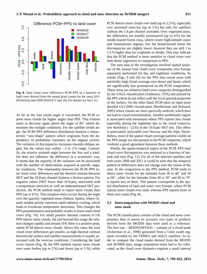
J. P. Musial et al.: Probabilistic approach to cloud and snow detection on AVHRR imagery 811

NOAA16NOAA17NOAA18

−5.

0−

2.5

0.0

2.5

5.0

7.5

wat

er

land

dese

rt

ice/

snow

need

le−

leav

e

broa

d−le

ave

crop

land

shru

bsPC

M −

PP

S [%

]

Difference PCM−PPS vs land cover

Fig. 8. Total cloud cover differences PCM–PPS as a function ofland cover derived from the annual pixel counts for the years 2011(NOAA16) and 2008 (NOAA17 and 18). For details see Sect.4.1.

As far as the Sun zenith angle is concerned, the PCM re-ports more clouds for higher angles than PPS. This relationstarts to decrease again above the angle of 85◦ which de-termines the twilight conditions. For the satellite zenith an-gle, the PCM–PPS difference distribution features a charac-teristic “saw-shape” pattern which originates from the de-pendency of probability estimates on the angular sectors.The variation of discrepancies increases towards oblique an-gles, but the values stay within−2 to 2 % range. Contrar-ily, the relative azimuth angle between the Sun and a satel-lite does not influence the difference in a systematic way.It seems that the majority of the variation can be associatedwith the number of observations acquired at specific angu-lar conditions. The relationship between the PCM–PPS to-tal cloud cover differences and the thermal contrast betweenSKT and the 10.8 µm channel features a distinct pattern. Fornegative values (SKT lower than 10.8 µm), associated witha temperature inversion or with an underestimated SKT pre-diction, the PCM method tends to report more clouds thanPPS (up to 8 %). This situation often occurs during the nightover the sparsely vegetated areas (Sahara, Spain), where cli-mate models poorly represent rapid radiative cooling, whichleads to erroneous temperature inversions. This changes thePPS parametrisation and probably results in lower total cloudcover (Fig.10). For small positive thermal contrast 0–5 KPPS reports more clouds, but just beyond this range the rela-tion changes rapidly and around 10 K there is a positive peak,where PCM detects more clouds. Above this value the totalcloud cover differences get smaller, as high thermal contrastbetween the surface and satellite measurements is usually as-sociated with the overcast conditions. Considering the landcover classes (Fig.8), the PPS method reports more cloudsover water bodies (up to 2 %) and desert (up to 5 %), while

PCM detects more clouds over land (up to 2.5 %), especiallyover perennial snow/ice (up to 5 %) but only for satelliteswithout the 1.6 µm channel activated. Over vegetated areas,the differences are notably pronounced (up to 4 %) for theneedle-leaved forest class, which covers high-latitude zonesand mountainous regions. For the broad-leaved forest thediscrepancies are slightly lower; however they are still 1 to1.5 % higher than for croplands or shrubs. This may indicatethat the PCM method is more sensitive to cloud cover overdark dense vegetation in comparison to PPS.

The next step of the investigation involved spatial analy-ses of the annual total cloud cover composites over Europeseparately performed for day and nighttime conditions. Itsresults (Figs.9 and 10) for the PPS data reveal areas withunreliably high cloud coverage over desert and Spain, whichare significantly less pronounced on the PCM composition.These areas are related to land cover categories distinguishedby the USGS classification (Anderson, 1976) and utilised bythe PPS which do not reflect well the local spectral propertiesof the surface. On the other hand, PCM takes as input moredetailed GLC2000 classification (Bartholomé and Belward,2005) where classes are more spectrally uniform, which doesnot lead to cloud overestimation. Another problematic regionis associated with mountains where PPS reports less cloudsespecially during the nighttime due to the cloud conserva-tive threshold (−22 K) in the 10.8 µm–SKT test. This effectis particularly noticeable over Norway and the Alps. Never-theless, most of the spatial cloud coverage patterns visible onthe PPS image are also present in the PCM composite, whichconfirms a good agreement between these methods.

Finally, the spatio-temporal aspect of the PCM–PPS totalcloud cover discrepancies was analysed as a function of lati-tude and time (Fig.11). For all of the selected satellites andboth years 2008 and 2011 it could be seen that the temporalpattern of differences does not change over the coarse of theyear. In the comparison to the PPS method, PCM tends todetect more clouds for the latitudes from 30 to 40◦ and 50to 60◦, while for the latitudes from 40 to 50◦ and 60 to 70◦

it reports less of them. This pattern corresponds to the spa-tial distribution of land and water over Europe, where PCMreports more clouds over land, whereas PPS reports more ofthem over water (Fig.8).

4.2 Intercomparison with MODIS cloud andsnow mask

The PCM classification consists of the cloud and snow com-ponents; thus to assess its accuracy two types of productsderived from the MODIS data were used as a reference.The first one – MOD35/MYD35 – consists of a cloud mask(Ackerman et al., 1998) generated from a 5 min swath seg-ment recorded by the TERRA and AQUA satellites. In or-der to compare the cloud masks derived from the MODISand AVHRR data, image acquisition times had to be collo-cated, as the cloud cover dynamics requires a small interval

www.atmos-meas-tech.net/7/799/2014/ Atmos. Meas. Tech., 7, 799–822, 2014

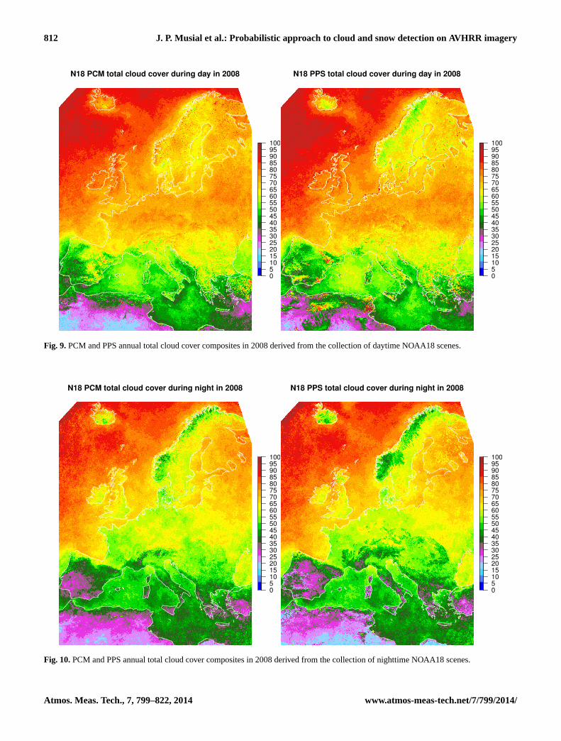
812 J. P. Musial et al.: Probabilistic approach to cloud and snow detection on AVHRR imagery

0

5

10

15

20

25

30

35

40

45

50

55

60

65

70

75

80

85

90

95

100

N18 PCM total cloud cover during day in 2008

0

5

10

15

20

25

30

35

40

45

50

55

60

65

70

75

80

85

90

95

100

N18 PPS total cloud cover during day in 2008

Fig. 9.PCM and PPS annual total cloud cover composites in 2008 derived from the collection of daytime NOAA18 scenes.

0

5

10

15

20

25

30

35

40

45

50

55

60

65

70

75

80

85

90

95

100

N18 PCM total cloud cover during night in 2008

0

5

10

15

20

25

30

35

40

45

50

55

60

65

70

75

80

85

90

95

100

N18 PPS total cloud cover during night in 2008

Fig. 10.PCM and PPS annual total cloud cover composites in 2008 derived from the collection of nighttime NOAA18 scenes.

Atmos. Meas. Tech., 7, 799–822, 2014 www.atmos-meas-tech.net/7/799/2014/

J. P. Musial et al.: Probabilistic approach to cloud and snow detection on AVHRR imagery 813

Fig. 11.Distribution of latitudinal total cloud cover differences be-tween the PCM and PPS algorithms throughout the years 2011 and2008 for the selected satellites. For details see Sect.4.1.

between spectral measurements. In this study the maximumtime difference was set to 15 min. Out of the three selectedNOAA platforms only the one labelled with number 18 wasused for the comparison. In the case of the NOAA16 in theyear 2011 the orbital drift was substantial; thus no colloca-tions were possible with TERRA/AQUA. For the NOAA17,match-ups should occur for high latitudes; however thosescenes were beyond the range of the receiving station antennalocated in Bern (Switzerland). Over Europe for the year 2008after the image collocations the combined AVHRR/MODISdata set consisted of 118 TERRA scenes and 238 AQUAscenes for both day and night conditions. Furthermore, the

MODIS product was modified to exclude the uncertain pixelcategory and to reclassify the confident/probably clear cat-egories to clear-sky class, as well as the confident/probablycloudy categories to overcast class.

Regarding the MOD/MYD35 product, the comparativeanalyses were performed analogically to the ones describedin the previous subsection. First, the total cloud cover overeach scene was computed for both cloud masking algorithmsto compose a scatter plot (Fig.12a). It occurs that on averagethe MODIS product reports 4.4 % more clouds than PCM re-maining at the same time with the high correlation of 0.95.Further, the PCM–MODIS total cloud cover discrepancieswere analysed as a function of land cover, Sun zenith angleand the SKT–10.8 µm thermal contrast (Fig.12b, c and d).The obtained results show that the PCM constantly reportsless clouds regardless of the land cover class with the high-est difference for the perennial snow/ice areas (up to 12 %).As far as the Sun zenith angle is concerned, the absolute dif-ferences increase almost linearly, and the best agreement be-tween the methods (±2.5 %) is reported for the SZA< 55◦.On the other hand, for the twilight conditions (SZA≥ 85◦)total cloud cover discrepancies between PCM and MOD35reach 10 %. Their relationship with the SKT–10.8 µm ther-mal contrast (Fig.12d) resembles the one from the PPS com-parison. When the surface temperature is lower than satellitemeasurements, PCM reports more clouds (up to 5 %). For thethermal difference in the 0 to 5 K range the PCM–MODISabsolute discrepancies increase (up to 18 %) and then dimin-ish rapidly, and above the 10 K both algorithms report thesame amount of clouds.

The MOD10A1 product (Hall et al., 2002) utilised as areference for the PCM classification consists of daily snowcover composites retrieved from the TERRA satellite data.As it is one of the few globally available snow cover datawith high spatial and temporal resolutions, in this study itwas regarded as ground-truth information. On the basis ofthe MOD10A1 and PCM products the contingency table wasconstructed (Eq.5), which allows computation of the follow-ing classification quality indicators (Eqs.6–11): probabilityof detection (POD), false alarm rate (FAR), hit rate (HR),and Kuipers skill score (KSS). The acquired results indicatethat the difference in estimated snow cover between the PCMand MOD10A algorithms is significant (Fig.14). Consider-ing the PCM snow detection skills, the highest, POD≈ 0.6,is reported for the NOAA17 which has the 1.6 µm channelactivated. On the other hand, the AVHRR sensors aboard theNOAA16,18 satellites with the 3.7 µm channel constantly op-erating feature lower snow detection skills: POD≈ 0.4. Theprevailing snow-free conditions over the coarse of the yearresult in extremely high POD, HR and low FAR for this cat-egory, due to unbalanced data counts within the contingencytable. In such a case, the KSS indicator should be utilised, asit objectively estimates the overall algorithm performance.Further, the total snow cover scatter plots, derived analog-ically to the ones from the cloud coverage analyses, were

www.atmos-meas-tech.net/7/799/2014/ Atmos. Meas. Tech., 7, 799–822, 2014

814 J. P. Musial et al.: Probabilistic approach to cloud and snow detection on AVHRR imagery

●●

●

●

●

●

●

●

●

●

●

●

●

●

●

●

●

●

●

●

●

●

●

●

●

●

●

●

●

●

●

●

●

●

●

●

●

●●

● ●●

●

●

●

●

●

●

●

●

●

●

●

●

●

●

●

●

●

●

●

●

●

●

●

●

●

●

●

●

●

●

●

●

●●

●

●

●

●

●

●

●

●

●

●

●

●

●

●

●

●

●

●

●

●

●

●

●

●

●

●

●

●

●

●

●●

●

●

●

●

●

●●

●

●

●

●

●

●

●

●

●

●

●

●

●

●

●

●

●

●

●

●

●

●

●

●

●

●

●

●

●

●

●

●

●●

●

● ●

●

●

●

●

●

●

●

●

●

●

●

●

●

●

●

●

●

●

●

●

●

●

●

●●

●

●

●

●

●

●●

●

●

●

●

●

●

●

●

●

●●

●

●

●

●

●

●

●

●

●

●●

●

●

●

●

●

●

●

●

●

●●

●

●

●●●

●●

●

●●

●

●

●

●●

●

●

●●

●

●

●

●

●

●

●●

●

●

●

●●

●

●

●

●

●

●

20 40 60 80 100

2040

6080

100

PCM [%]

MO

D35

[%]

Total cloud cover NOAA18 PCM vs MOD35

R2 = 0.95PCM−MOD35

mean = −4.38

stdev = 5.54

median = −3.46

a)

0.0e

+00

5.0e

+06

1.0e

+07

1.5e

+07

2.0e

+07

20 30 40 50 60 70 80 90

c)

Difference NOAA18 PCM−MOD35 vs SUNZ

coun

ts

Sun zenith angle [degree]

PC

M −

MO

D35

[%]●●●●●●●●

●

●

●

●

●

●

●

●

●

●●●

●●

●●

●

●

●●●●●●●●●●●●●●●

●●●●●●●●●●●

●●●●●●

●●●●●

●●●

●●●●●●●

●●●●●●●●

●

●●

●

●●

●

●●●

●●●●

●●●●●

●

●●●

−15

.0−

10.0

−5.

00.

02.

55.

0

0e+

002e

+07

4e+

076e

+07

8e+

071e

+08

−15 −5 0 5 10 15 20 25 30

d)

Difference NOAA18 PCM−MOD35 vs SKT−ch4

coun

ts

Temperature diff. SKT−ch4 [K]

PC

M −

MO

D35

[%]

●

●●●●●●

●●

●●

●●

●●

●

●

●

●

●

●●

●

●●

●●●●●●●●●●●●●●●●●●●●

−30

−20

−10

010 NOAA18

−15

−10

−5

05

10

wat

er

land

dese

rt

ice/

snow

need

le−

leav

e

broa

d−le

ave

crop

land

shru

bs

PC

M −

MO

D35

[%]

Difference NOAA18 PCM−MOD35 vs land cover

b)

Fig. 12.Differences in total cloud cover between PCM and MOD/MYD35 products derived from annual pixel counts of the NOAA18 satellitefor the year 2008:(a) computed over each scene,(b) as a function of land cover,(c) as a function of Sun zenith angle,(d) as a function ofthermal differences between SKT and 10.8 µm channel. Red lines denote trend, and data frequency is presented as grey-shaded histograms.For details see Sect.4.2.

computed (Fig.13d, h and l). The obtained results show thatPCM reports significantly less snow cover (up to 9.5 % onaverage) than MOD10A1, with a moderate correlation coef-ficient (0.5–0.7) and a high standard deviation (up to 17 %).The absolute PCM–MOD10A1 total snow cover differencesincrease with the Sun zenith angle up to 85◦, where theyslightly decrease due to separate treatment of the twilightconditions (Fig.13a, e and i). The relationship with the satel-lite zenith angle indicates that PCM reports more snow athigh angles, possibly due to increasing instrument field ofview (FOV), but only for the NOAA16 and 17 platforms.The opposite trend for the NOAA18 satellite is not easily ex-plainable and might be related to geographic distribution ofsnow in Europe, which is most persistent over the Alps andScandinavia. These regions are located around the centre ofa swath of the NOAA18 satellite; thus the amount of snowpixels across the scan is not even. The PCM–MOD10A1 to-tal snow cover differences vary with the relative azimuth an-gle according to a pattern mostly related to the quantity ofavailable observations. Nevertheless, for the NOAA18 thereis a significant increase of discrepancies around the azimuth

angle of 60◦ (towards forward scattering), which once moremight be associated with combined geographical and angularconditions rather than the algorithm’s configuration.

counts PCM clear PCM snowMODIS clear a b

MODIS snow c d

(5)

PODsnow =d

c + d(6)

PODclear =a

a + b(7)

FARsnow =b

b + d(8)

FARclear =c

a + c(9)

HR =a + d

a + b + c + d, where 0≤ HR ≤ 1 (10)

KSS =a × d − c × b

(a + b) × (c + d), where− 1 ≤ KSS ≤ 1 (11)

Atmos. Meas. Tech., 7, 799–822, 2014 www.atmos-meas-tech.net/7/799/2014/

J. P. Musial et al.: Probabilistic approach to cloud and snow detection on AVHRR imagery 815

0e+

002e

+07

4e+

07

40 50 60 70 80 90

a)

coun

ts

Sun zenith angle [degree]

PC

M −

MO

D10

A1

[%]

NOAA16

●●●●●●●●●●●●●●●●●●●●●●●●●●●●●●●●●●●●●●●●●●●●●●●●●

●●●●

−30

−20

−10

−5

05

0.0e

+00

1.0e

+07

2.0e

+07

3.0e

+07

0 10 20 30 40 50 60 70

b)

coun

ts

Satellite zenith angle [degree]

PC

M −

MO

D10

A1

[%]

●●●●●●●●●●●●●●●●●●●●●●●●●●●●●●●●●●●

●●●●●

●●●●●●●●●●

●●●●●●

●●●●

●●●●●●●●

●

●

−8

−6

−4

−2

0

0e+

001e

+07

2e+

073e

+07

4e+

07

0 30 60 90 120 180

c)

coun

ts

Relative azimuth angle [degree]

PC

M −

MO

D10

A1

[%]

●

●●●●●●●●●●

●

●●●

●

●

●

●

●

●

●

●

●●●●

●●●●●●●●●●●●●●

●●●●

●●●●●●●●●●●●●●●●●●●●

●●●●●●●●●

●●●●●●●●●●●●●●●●

●●●●●●●●●●●●●●●●●●●●●●●●●●●●

●●●●●●●●●●●●●●●●●●●

●●

●●●●●●●●

●●●●●●●

●●●●●

●

●

●

●

●

●

●

●

●

●

●

●●●●●●●●●●●

−30

−20

−10

−5

05

●

●

●

●

●

●

●

●

●

●

●

●●●● ●● ●

●

●

●

●●

●

●

● ●

●

●

●

●

●

●●

●

●

●

●

●

●

●

● ●

●

●

●

●●

●

● ●

● ●●

●

●

●

●

●

●

●

●●

●

●

●

●

●

●

●

●

●

●●

●

●

●

●

●

●

●

●

●

●

●

●●

●

●

●

●

●

●

●●

●

●

●

●

●

●

●

●

●

●

●

●

●

●

●

●

●

●

●

●

●

●

●

●

●

●

●

●

●

●

●

●

●

●

●

●

●

●

●

●

●

●

●●

●

●

●

●

●

●

●

●

●

●

●

●

●

●

●

●

●

●

●

●

●

●●

●

●●

●

●

●

●

●

●

●

●●

●

●●●

●

●

●

●

●●

●

●●

●

●●●●

●

●

●●●

●●●●

●

●●

●●●●

●

●● ●●

●

●●

●

●●

●

●●

●

●

●

●●●●●●

●

●●●●●●●●

●●

●

●●●

●●

●●

●

●●

●

●●●●●●●●●●●●●

●

●●

●●●

●●

●●●●●●●●●●●●●●●●●●●●●●●●●●●●●●●●●●●●●●●●●●●●●●●●●●●●●●●●●●●●

●

●●●●●●●●●●●●●●●●●●●●●●●●●●●●●●●●●●●●●●●●●●●●●●●●●●●●●●●●●●●●●●●●●●●●●●●●●●●●●●●●●●●●●●●●●●●●●●●●●●●●●●●●●●●●●●●●●●●●●●●●●●●●●●●●●●●●●●●●●●●●●●●●●●●●●●●●●●

●

●●●●●●

●●●●●●●●●●●●●●

●

●●

●

●●●

●●●●●●●●

●●●●●●●●●

●

●●●●●●●●●●●●●●●●●●●●●

●

●

●

●

●●

●

●●

●

●

●

●●●●●

●●●●●●●●

●

●

●

●

●

●●

●

●

●

●

●

●

●

●

●

●

●

●●●

●

●

●

●●●●

●●●

●

●

●

●

●

●

●

●

●

●

●

●●●●●●

●●

●

●

●

●

●

●●●●●●

●●●●●●

●

●

●●

●

●●●●●

●●●

●●

●

●●●

●●

●

●

●

●●●

●

●

●● ●●

●

●

●

●●●●●

●●●

●

●●●●

●

●

●

●●

●

●

●●●

●

●

●

●●●

●

●●

●●

●●

●●●

●

●●

●

●

●●

●●

●●

0 10 20 30 40 50 60 70

010

2030

4050

6070

PCM [%]

MO

D10

A1

[%]

d)

R2 = 0.75

PCM−MOD10A1

median = −1.80

mean = −6.55

stdev = 12.65

0e+

002e

+07

4e+

07

40 50 60 70 80 90

e)

coun

ts

Sun zenith angle [degree]

PC

M −

MO

D10

A1

[%]

NOAA17Total snow cover difference PCM−MOD10A1

●●●●●●●●●●●●●●●●●●●●●●●●●●●●●●●●●●●●●●●●●●●●●●●●●●●●●●●●●●●●●●●●

●

●●●●

●●

●●

●

●

●

●

−30

−20

−10

−5

05

0.0e

+00

1.0e

+07

2.0e

+07

3.0e

+07

0 10 20 30 40 50 60 70

f)

coun

ts

Satellite zenith angle [degree]

PC

M −

MO

D10

A1

[%]

●●●●●●●●●●●●●●●●●●●●●●●●●●●●●●●●●●●●●●●●●●●●●●●●

●●●●●●●●●●●

●●●●●●●●●

●

−8

−6

−4

−2

0

0e+

001e

+07

2e+

073e

+07

4e+

07

0 30 60 90 120 180

g)

coun

ts

Relative azimuth angle [degree]

PC

M −

MO

D10

A1

[%]

●

●●●●●●●●●●●●●●●●●●●●●●●●●●●●●●●●●●●●●●●●●●●●●●●●●●

●

●●●●●●●●

●●●●●●●●●●●●●●●●●●●●●●●●●●●●●●●●●●●●●●●●●●●●●●●●●●●●●

●

●●●●●●●

●

●●●●

●●●●●●●●●

●●●●●●●●●●●●●●●●●●●●●●●●●●●●●●●●●●●●●●●●●●●●●●

−30

−20

−10

−5

05

●

●

●

●

●●

●

●

●

●

●

●

●

●

●

●

●●

●

●

●

●●●

●●

●

●●●

●●●

●

●

●●●

●

●

●

●●●

●

●●

●

●

●

●●

●

●

●

●●

●●

●

●

●

●

●

●●

●

●

●

●

●

●

●

●●●

●

●

●

● ●

●●●

●

●●

●

●

●

●●

●●

●●●

●●●●

●

●●●

●

●●

●●

●

●●

●

●●

●●

●●

●

●●

●

●

●

●

●

●●

●

●●

●

●

●

●

●

●

●

●

●

●

●

●

●

●

●

●●

●

●

●

●

●

●

●

●

●

●●

●

●

●

●

●

●

●

●

●

●●

●

●

●

●

●

●

●

●

●●

●

●●

●

●

●

●

●

●

●

●

●●

●

●

●

●

●

●

●

●●

●

●●

●

●●

●

●

●

●

●

●

●●

●

●

●

●

●

●

●

●

●

●●

●

●●

●

●

●

●

●

●

●

●●

●

●●●

●

●

●

●●

●

●

●●

●

●

●

●

●

●

●

●

●

●●

●

●●

●

●

●

●

●

●

●

●●

●

●●

●

●

●

●

●●

●

●

●

●●

●

●

●

●

●●

●

●

●

●●●

●●

●

●

●

●●

●

●●

●

●

●

●

●

●

●

●

●●●

●

●

●

●

●

●

●

●

●●

●

●●

●

●●

●

●●

●

●●

●

●●●●●

●

●

●●

●● ●●

●

●●

●●

●●●●●●

●

●

●

●

●●

●

●

●●●

●

●●●

●

●

●

●

●

●●●●●

●

●

●●

●

●●

●

●●

●

●●●

●●

●

●●●●●●●

●

●

●●

●●

●

●

●

●●

●

●

●

●●●

●

●●

●

●●

●

●●

●

●

●

●●

●●

●

●

●●

●

●

●

●●

●

●●

●

●●

●

●●

●

●

●

●

●

●●●

●

●●

●

●

●

●●

●

●●●●●●●● ●●

●

●●●●●●●●●●●●●●●●●●●●●●●●●●●●●●●●●

●●●●●●●●●●●●

●●●●●●

●●●●●

●●●●

●

●●

●●●

●

●

●

● ●

●

●

●

●

●

●

●●

●●●●●●●●●●●●●

●

●

●●

●●

●

●

●●●

●

●●

●●

●●●

●

●

●

●

●● ●●

●●●

●

●

●●

●●

●

●

●●

● ●●

●

●

●

●

●

●

●

●●

●

●●

0 10 20 30 40 50 60 70

010

2030

4050

6070

PCM [%]

MO

D10

A1

[%]

h)

R2 = 0.59

PCM−MOD10A1

median = −3.45

mean = −7.52

stdev = 14.82

0e+

002e

+07

4e+

07

40 50 60 70 80 90

i)

coun

ts

Sun zenith angle [degree]

PC

M −

MO

D10

A1

[%]

NOAA18

●●●●●●●●●●●●●●●●●●●●●●●●●●●●●●●●●●●●●●●●●●●●●●●●●●●●●●●●

●●●●●●●

●●●

●

●

●●●

●●●●●●

●

●●

●

●

●

−30

−20

−10

−5

05

0.0e

+00

1.0e

+07

2.0e

+07

3.0e

+07

0 10 20 30 40 50 60 70

j)

coun

ts

Satellite zenith angle [degree]

PC

M −

MO

D10

A1

[%]

●●●●●●●●●●●●●●●●●●●●●●●

●●●●●●●●●●●●●●●●●●●●●●●●

●●●●●●●●●●●●

●●●●●●

●●●

●

●

−8

−6

−4

−2

0

0e+

001e

+07

2e+

073e

+07

4e+

07

0 30 60 90 120 180

k)

coun

ts

Relative azimuth angle [degree]

PC

M −

MO

D10

A1

[%]

●

●●●●●●●●●●●●●●●●●●●●●●●●●●●●●●●●●●●●●●●●●●●●●●●●●●●●●●●●●

●

●●●●●●

●

●

●

●

●●

●

●

●●

●●

●●●●●●●●●●●●●●●●●●●●●●●●●●●●●●●●

●●●●●●●●●●●●

●●●●●●●●●●●●●●

●●●●●●●●●●●●●●●●●●●●●●●●●●●●●●●●●●●●●●●●●●●●●●

−30

−20

−10

−5

05

●

●

●

●

●

●

●

●

●

●

●

●

●

●●

●●

●●

●

●

●

●

●

●

●●●

●●

●

●

●

●

●

●

●

●

●

●

●

●●

●●

●●

●

●

●

●

●

●

●

●

●●●

●

●

●

●

●

●

●

●

●

●

●

●

●

●●

●

●

●

●

●

●

●

●

●

●

●

●

●

●

●●

●

●

●

●

●

●

●●●

●●●

●

●

●

●

●

●

●

●

●

●●●

●

●

●●

●

●

●

●

●

●

●

●

●

●

●●

●

●

●

●

●

●

●

●●

●

●●

●

●

●

●

●

●

●

●

●

●

●

●●

●

●

●

●

●

●

●

●

●

●

●

●

●

●

●

●

●

●

●

●

●

●

●●

●

●

●

●

●

●

●

●

●

●

●

●

●

●

●

●

●

●

●

●

●

●

●

●

●

●

●

●

●

●

●

●

●

●

●

●●

●

●●

●

●

●

●

●●

●

●●

●

●

●

●

●

●

●

●

●

●

●

●

●

●

●●

●

●●

●

●●

●

●●

●

●

●

●

●

●

●

●

●

●

●●

●

●

●

●

●●●●●

●●●

●

●●

●

●●

●

●

●

●

●

●

●●

●●

●

●

●●●●● ●●●●●●●●●

●

●●

●

●●●

●●●

●●●●●●●●●●●● ●●●●

●●●●●●●

●●●●●●●●●●●

●●●●●●●●●●●●●●●●●●●●●●●● ●●●●● ●●●●●●●●●●●●●

●●

●●●●●●

●

●●●●●●●●●●●●

●● ●●● ●● ●●●●

●●

●

●●●

●

●●

●

●● ●●● ●●●

●●●●●

● ●●●●●●●●●●●●●●●● ●●●●●●●●●

●

●●●●●●●●●●●●●●●●●●●●●●●●●●●●●●●●●●●●●●●●●

●●

●

●

●●

●

●●●●●●●●●●●●●●●●●●

●

●●●

●●

●●●●●●●●●

●●

●

●

●

●

●

●●

●

●

●●●

●

●

●

●●●

●●

●

●

●●

●●●

●●

●

●

●

●

●

●

●

●

●●

●

●

● ● ●

●

●

●

●

●

●

●

●

●

●

●

●

●

●

●

●

●

●

●

●

●

●

●●

●●

●

●

●●

●

●

●

●

●

●

●

●

●

●

●

●

●

●

●

●

●

●

●

0 10 20 30 40 50 60 70

010

2030

4050

6070

PCM [%]

MO

D10

A1

[%]

l)

R2 = 0.63

PCM−MOD10A1

median = −3.27

mean = −7.97

stdev = 15.55

Fig. 13.Total snow cover difference PCM–MOD10A1 as a functionof selected variables derived from annual pixel counts for the years2011 (NOAA16) and 2008 (NOAA17 and 18). Data frequency ispresented as grey-shaded histograms. Bottom panels present the to-tal snow cover scatter plots derived from estimates computed overeach scene. Red lines denote trends. For details see Sect.4.2.

NOAA16NOAA17NOAA18

0.0

0.2

0.4

0.6

0.8

1.0

POD FAR POD FAR HR KSSSNOW CLEAR

PCM snow validation against MOD10A1

Fig. 14.Accuracy indicators of the PCM snow detection skills de-rived from the comparison with the MOD10A1 product. For detailssee Sect.4.2.

0 20 40 60 80 100

0.0

0.2

0.4

0.6

0.8

1.0

Normalised probability distribution

Probability [%]

cloudclearsnow

Fig. 15.PCM normalised probability distribution for clear, cloudyand snow conditions derived from annual counts of the NOAA18satellite data. For details see Sect.4.3.

4.3 Validation against SYNOP weather reports

The global network of SYNOP stations (Fig.16a) providesdetailed cloud cover observations acquired at high temporalresolution (up to one hour). They are collected in a consistentmanner during day and night for a long period, which makesthem an excellent validation source for the satellite-basedproducts. In this study SYNOP total cloud cover observa-tions expressed in octants were compared to the PCM cloudprobability, which was recoded to 0–100 % range, where0 % denotes confident clear/snow class and 100 % indicatesconfident cloudy category. In order to maintain the coher-ence between these data sets, the PCM outputs in a binaryform (clear/cloudy) and the cloud probability were averagedwithin the 30 km buffer zone around each station. This areashould correspond to the sky extent usually visible to an ob-server at the station (Karlsson, 1995). Analogically to thecomparison with the MOD/MYD35 data, the satellite andground cloud observations were collocated within the 15 mininterval. Next, the mean PCM cloud probability was com-puted as functions of the SYNOP cloud amount and time ofday from all of the collocated stations and satellites in theselected years (Fig.16b–d). The acquired probability dis-tributions span from around 12 % for completely clear-skySYNOP observations to 90 % for fully overcast conditionsregardless of the time of day. Furthermore, the histograms ofannual normalised probability distributions for clear, cloudyand snow conditions were computed (Fig.15). Their shapevery well corresponds to other probabilistic cloud mask dis-tributions enclosed in the studies ofGómez-Chova et al.(2007) andHeidinger et al.(2012).

In order to compute the quality indicators (Eqs.5–11withcloudy instead ofsnow) the PCM and PPS cloud fractions de-rived over the 30 km buffer zone together with the SYNOP

www.atmos-meas-tech.net/7/799/2014/ Atmos. Meas. Tech., 7, 799–822, 2014

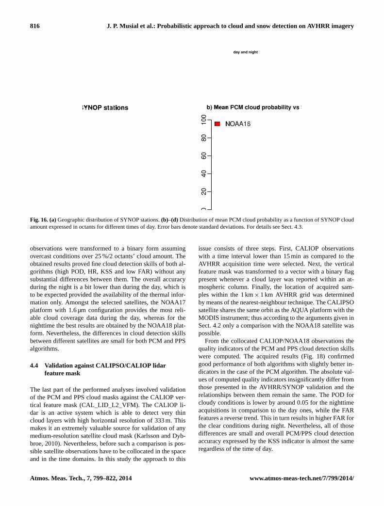
816 J. P. Musial et al.: Probabilistic approach to cloud and snow detection on AVHRR imagery

day and night

Fig. 16. (a)Geographic distribution of SYNOP stations.(b)–(d) Distribution of mean PCM cloud probability as a function of SYNOP cloudamount expressed in octants for different times of day. Error bars denote standard deviations. For details see Sect.4.3.

observations were transformed to a binary form assumingovercast conditions over 25 %/2 octants’ cloud amount. Theobtained results proved fine cloud detection skills of both al-gorithms (high POD, HR, KSS and low FAR) without anysubstantial differences between them. The overall accuracyduring the night is a bit lower than during the day, which isto be expected provided the availability of the thermal infor-mation only. Amongst the selected satellites, the NOAA17platform with 1.6 µm configuration provides the most reli-able cloud coverage data during the day, whereas for thenighttime the best results are obtained by the NOAA18 plat-form. Nevertheless, the differences in cloud detection skillsbetween different satellites are small for both PCM and PPSalgorithms.

4.4 Validation against CALIPSO/CALIOP lidarfeature mask

The last part of the performed analyses involved validationof the PCM and PPS cloud masks against the CALIOP ver-tical feature mask (CAL_LID_L2_VFM). The CALIOP li-dar is an active system which is able to detect very thincloud layers with high horizontal resolution of 333 m. Thismakes it an extremely valuable source for validation of anymedium-resolution satellite cloud mask (Karlsson and Dyb-broe, 2010). Nevertheless, before such a comparison is pos-sible satellite observations have to be collocated in the spaceand in the time domains. In this study the approach to this

issue consists of three steps. First, CALIOP observationswith a time interval lower than 15 min as compared to theAVHRR acquisition time were selected. Next, the verticalfeature mask was transformed to a vector with a binary flagpresent whenever a cloud layer was reported within an at-mospheric column. Finally, the location of acquired sam-ples within the 1 km× 1 km AVHRR grid was determinedby means of the nearest-neighbour technique. The CALIPSOsatellite shares the same orbit as the AQUA platform with theMODIS instrument; thus according to the arguments given inSect.4.2 only a comparison with the NOAA18 satellite waspossible.

From the collocated CALIOP/NOAA18 observations thequality indicators of the PCM and PPS cloud detection skillswere computed. The acquired results (Fig.18) confirmedgood performance of both algorithms with slightly better in-dicators in the case of the PCM algorithm. The absolute val-ues of computed quality indicators insignificantly differ fromthose presented in the AVHRR/SYNOP validation and therelationships between them remain the same. The POD forcloudy conditions is lower by around 0.05 for the nighttimeacquisitions in comparison to the day ones, while the FARfeatures a reverse trend. This in turn results in higher FAR forthe clear conditions during night. Nevertheless, all of thosedifferences are small and overall PCM/PPS cloud detectionaccuracy expressed by the KSS indicator is almost the sameregardless of the time of day.

Atmos. Meas. Tech., 7, 799–822, 2014 www.atmos-meas-tech.net/7/799/2014/

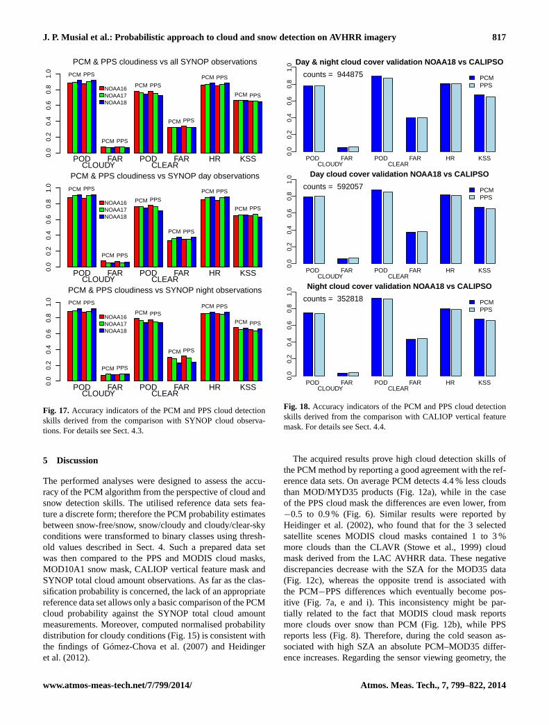
J. P. Musial et al.: Probabilistic approach to cloud and snow detection on AVHRR imagery 817

NOAA16NOAA17NOAA18

0.0

0.2

0.4

0.6

0.8

1.0

PCM PPS

PCM PPS

PCM PPS

PCM PPS

PCM PPS

PCM PPS

POD FAR POD FAR HR KSSCLOUDY CLEAR

PCM & PPS cloudiness vs all SYNOP observations

NOAA16NOAA17NOAA18

0.0

0.2

0.4

0.6

0.8

1.0

PCM PPS

PCM PPS

PCM PPS

PCM PPS

PCM PPS

PCM PPS

POD FAR POD FAR HR KSSCLOUDY CLEAR

PCM & PPS cloudiness vs SYNOP day observations

NOAA16NOAA17NOAA18

0.0

0.2

0.4

0.6

0.8

1.0 PCM PPS

PCM PPS

PCM PPS

PCM PPS

PCM PPS

PCM PPS

POD FAR POD FAR HR KSSCLOUDY CLEAR

PCM & PPS cloudiness vs SYNOP night observations

Fig. 17. Accuracy indicators of the PCM and PPS cloud detectionskills derived from the comparison with SYNOP cloud observa-tions. For details see Sect.4.3.

5 Discussion

The performed analyses were designed to assess the accu-racy of the PCM algorithm from the perspective of cloud andsnow detection skills. The utilised reference data sets fea-ture a discrete form; therefore the PCM probability estimatesbetween snow-free/snow, snow/cloudy and cloudy/clear-skyconditions were transformed to binary classes using thresh-old values described in Sect.4. Such a prepared data setwas then compared to the PPS and MODIS cloud masks,MOD10A1 snow mask, CALIOP vertical feature mask andSYNOP total cloud amount observations. As far as the clas-sification probability is concerned, the lack of an appropriatereference data set allows only a basic comparison of the PCMcloud probability against the SYNOP total cloud amountmeasurements. Moreover, computed normalised probabilitydistribution for cloudy conditions (Fig.15) is consistent withthe findings ofGómez-Chova et al.(2007) and Heidingeret al.(2012).

POD FAR POD FAR HR KSS

PCMPPS

Day & night cloud cover validation NOAA18 vs CALIPSO

CLOUDY CLEAR

0.0

0.2

0.4

0.6

0.8

1.0

counts = 944875

POD FAR POD FAR HR KSS

PCMPPS

Day cloud cover validation NOAA18 vs CALIPSO

CLOUDY CLEAR

0.0

0.2

0.4

0.6

0.8

1.0

counts = 592057

POD FAR POD FAR HR KSS

PCMPPS

Night cloud cover validation NOAA18 vs CALIPSO

CLOUDY CLEAR

0.0

0.2

0.4

0.6

0.8

1.0

counts = 352818

Fig. 18. Accuracy indicators of the PCM and PPS cloud detectionskills derived from the comparison with CALIOP vertical featuremask. For details see Sect.4.4.

The acquired results prove high cloud detection skills ofthe PCM method by reporting a good agreement with the ref-erence data sets. On average PCM detects 4.4 % less cloudsthan MOD/MYD35 products (Fig.12a), while in the caseof the PPS cloud mask the differences are even lower, from−0.5 to 0.9 % (Fig.6). Similar results were reported byHeidinger et al.(2002), who found that for the 3 selectedsatellite scenes MODIS cloud masks contained 1 to 3 %more clouds than the CLAVR (Stowe et al., 1999) cloudmask derived from the LAC AVHRR data. These negativediscrepancies decrease with the SZA for the MOD35 data(Fig. 12c), whereas the opposite trend is associated withthe PCM−PPS differences which eventually become pos-itive (Fig. 7a, e and i). This inconsistency might be par-tially related to the fact that MODIS cloud mask reportsmore clouds over snow than PCM (Fig.12b), while PPSreports less (Fig.8). Therefore, during the cold season as-sociated with high SZA an absolute PCM–MOD35 differ-ence increases. Regarding the sensor viewing geometry, the

www.atmos-meas-tech.net/7/799/2014/ Atmos. Meas. Tech., 7, 799–822, 2014

818 J. P. Musial et al.: Probabilistic approach to cloud and snow detection on AVHRR imagery

comparison against MODIS data is not conclusive as bothinstruments (AVHRR and MODIS) measure the same areaunder different angles. Therefore, such an analysis was per-formed only with the PPS algorithm, which relies on thesame AVHRR input data as the PCM. The distribution of to-tal cloud cover differences as a function of satellite zenithangle features a characteristic saw-shape pattern (Fig.7b, fand j), which originates from the division of angles’ valuesinto sectors. It can be presumed that without this partitioningthe differences between PCM and PPS methods would risecontinuously and the overall discrepancies between the algo-rithms would be higher. The relationship of the differenceswith the Sun–satellite relative azimuth angle does not revealany significant pattern, and the noticeable variations might beattributed to the quantity of available observations (Fig.7c,g and k). However, the distribution of total cloud cover dis-crepancies related to the thermal contrast between SKT andthe 10.8 µm BT has a distinct drop of values within the 0 to10 K range for both PPS and MODIS comparisons (Figs.7b,f, j and 12d). This effect could be partially associated withthe different approach towards local radiance variation anal-ysis over water bodies, where PPS and MOD35 mark a pixelas cloudy whenever the spectral variance in its vicinity (e.g.5× 5 window) is sufficiently high (Di Vittorio and Emery,2002). However, this implies that some of the clear-sky pixelsaround cloud edges with small thermal contrast are misclas-sified. In the PCM method the textural analysis is performeddifferently by means of the kernel convolution with a smallwindow (Eq.1), which assures that only pixels at cloud edgesare detected. Therefore, the PPS and MOD35 products reportmore clouds than PCM over water bodies (Figs.8 and12b),which in turn modifies the overall results significantly, as it isthe most extensive land cover class. This is also confirmed bythe spatio-temporal analysis of the total cloud cover differ-ences between the PCM and PPS methods (Fig.11). For thelatitude ranges of 40–50◦ and 60–70◦, where the water classis predominant over the study area, the PPS algorithm reportsmore clouds than PCM regardless of the time of the year. Forother surfaces the total cloud cover difference remains neg-ative in the case of the comparison with the MODIS data,whereas comparison with the PPS data, the PCM algorithmtends to report more clouds over the land surfaces excludingdeserts. The same relationships could be observed on the an-nual total cloud cover composites for the NOAA18 satellite(Figs.9 and10). Moreover, the daytime PPS composite con-tains artefacts associated with areas characterised by the un-reliably frequent cloud cover (up to 100 %) over Africa andSpain. They are related to land cover classes described byAnderson(1976) which do not resolve well the local spec-tral characteristics and lead to overestimation of the cloudamount. These areas are less apparent on the PCM total cloudcover composite because the PCM algorithm utilises moredetailed land cover categorisation (Bartholomé and Belward,2005). Furthermore, the PPS-based training data set was cor-rected by an analyst before being utilised during the PCM

development phase. Another noticeable spatial difference isassociated with mountains (e.g. Alps), where PCM reportsmore clouds than PPS especially during the nighttime. Thisis related to the fact that in the PPS method the SKT–10.8 µmthermal contrast test features very cloud conservative thresh-old (22 K at night) over the rough topography areas. This wasintroduced to account for the temperature variability inducedby the comparison of 1 km× 1 km AVHRR data with low-resolution SKT estimates (Dybbroe et al., 2005a). Neverthe-less, due to this relaxed threshold the SKT–10.8 µm test oftenindicates clear-sky conditions, which misleads the PPS algo-rithm, and results in lower cloud coverage over the moun-tainous regions.

In order to evaluate the accuracy of the PCM and PPSalgorithms, the total cloud cover observations provided bythe SYNOP stations (Fig.16a) were compared to the PCMand PPS cloud fractions derived over the 30 km buffer zonearound each station. This analysis involved creation of thecontingency table and computation of the classification qual-ity indicators (Eqs.5–11). They are the same for both meth-ods or slightly better in the case of the PCM results (Fig.17).The small improvement over the PPS algorithm was gainedby the correction of the PPS/MOD10A1 training data set ap-plied by the analyst. High probability of detection (> 0.8)and low false alarm rate (< 0.1) for the cloudy conditions re-main at the same level for both algorithms regardless of thetime of the day. Lower detection skills for the clear-sky casescan be attributed to the fact that an observer at a SYNOPstation may report clouds which are further than the 30 kmdistance (for more comprehensive explanation seeKarlsson,1995). Nevertheless, the overall performance of both algo-rithms represented by the Kuipers skill score is high andthe differences between the selected satellites are inconsider-ably small. Furthermore, these results are consistent with theCALIOP/AVHRR validation (see Sect.4.4) from the quali-tative perspective; however their absolute values are higher.This is due to the fact that computation of fractional cloudcover within the 30 km buffer zone increases the probabilityof cloud detection. On the other hand, the CALIOP/AVHRRvalidation was performed on a single pixel basis, whichyields more accurate results. The high sensitivity of a lidarsystem to detection of thin clouds which are not visible forthe AVHRR sensor is well apparent as a relatively high FAR(> 0.4) for the clear conditions. This is also the reason forthe higher cloud amount in the cloud mask derived fromthe MODIS instrument which has 1.38 and 8.55 µm chan-nels that improve the detection of mid-level and high clouds(Ackerman et al., 1998). The acquired classification qualitycriteria for the CALIOP/PPS cloud mask comparison remainin a good agreement (within the 10 % range) with the studyof Karlsson and Dybbroe(2010), who performed the sameanalysis over the Artic region.

Within the 30 km buffer zones around each station themean PCM cloud probability was analysed as a functionof the SYNOP cloud amount (Fig.16b–d). The acquired

Atmos. Meas. Tech., 7, 799–822, 2014 www.atmos-meas-tech.net/7/799/2014/

J. P. Musial et al.: Probabilistic approach to cloud and snow detection on AVHRR imagery 819

distribution feature a reasonable spread of values from∼ 12 % for the clear-sky conditions to∼ 90 % for the fullyovercast sky, regardless of the time of the day and theAVHRR channel configuration. The acquired probability dis-tribution remains in a good consistency with the SYNOPvalidation results for the POLarization and Directionalityof the Earth’s Reflectances (POLDER) cloud mask (Bréonand Colzy, 1999). Although in that case the distribution ex-pressed the percentage of cloudy pixels as a function of theSYNOP cloud amount, the PCM probability estimates fea-ture almost a binary distribution (Fig.15), which fits wellto the binary output of the POLDER cloud mask. The samecharacteristics of the cloud probability distribution were re-ported in other studies (Gómez-Chova et al., 2007; Heidingeret al., 2012). Its specific “U shape”, where most of the pix-els are classified as confident clear 0 % or cloudy 100 %, isrelated to the high spectral contrast of clouds on a satelliteimage as compared to other surfaces (see red dots in Fig.2).Most of the classification probability estimates significantlydifferent than 0 or 100 % represent pixels with fractionalcloud and/or snow coverage, ice clouds overlaying a cold sur-face, and thin cirrus clouds. These cases are far less frequentthan fully overcast or clear-sky pixels, which results in highlypolarised probability distribution (Fig.15).

The snow component of the PCM output was validatedagainst the MOD10A1 daily composite, which is one of thefew existing snow cover data sets matching the spatial andtemporal resolution of the AVHRR data. Although the highaccuracy of this product was proven (Hall and Riggs, 2007),some misclassification especially between snow and cloudsor overestimation of snow in forests may influence the qual-ity indicators for the PCM method (Eqs.5–11). Moreover,it has to be taken into account while interpreting the resultsthat NOAA16 data were collected during the year 2011 whileNOAA17 and NOAA18 data originate from the year 2008.Thus, different snow cover conditions between these periodsinfluence the computed statistics. In this analysis only thecloud-free areas were considered; therefore some pixels atsnow cover edges (Fig.5), which are often misclassified asclouds (Hall and Riggs, 2007), were not taken into account.The best agreement between PCM and MOD10A1 total snowcover estimates is reported for the NOAA17 satellite whichhas the 1.6 µm channel activated. For the platforms with the3.7 µm channel constantly operating the discrepancies aremore significant. Although the POD of snow is considerablyhigher for the NOAA17 platform (Fig.14), the FAR indica-tor is on the same level for the NOAA18 satellite. Therefore,it can be concluded that the PCM classification results for theNOAA17 and 18 satellites are valuable in terms of the snowcomposite derivation. Nevertheless, the accuracy of the PCMsnow cover classification is strongly dependent on the illumi-nation conditions. It was found that for the NOAA17 and 18satellites the absolute PCM–MOD10A1 differences increasesignificantly above the Sun zenith angle of 70◦ (Fig. 13a, eand i). A similar value was reported bySolberg et al.(2010).

This effect is not that apparent for the NOAA16 satellite pos-sibly due to the different snow conditions in 2011 as com-pared to 2008.

The comparison and validation of the PCM results againstspace-borne and ground data proved the high cloud detec-tion skills. As far as the snow classification is concernedthe overall accuracy of the algorithm is reasonable, but spe-cial precaution has to be taken for data generated withoutthe 1.6 µm channel, especially for the high Sun zenith angleacquisitions. The lack of reference probability estimates forcloudy/clear-sky, cloudy/snow or snow/clear-sky conditionsallows only the comparison with the SYNOP cloud amount,which confirms the expected value spread with low proba-bilities (∼ 15 %) for the clear-sky conditions and high ones(∼ 90 %) for the fully overcast sky. Finally, the PCM cloudand snow classification was proven to be valid for a broadrange of environmental conditions across Europe and north-ern parts of Africa.

6 Conclusions

This study presents a robust algorithm for cloud and snow de-tection on AVHRR imagery which provides complementaryprobability estimates. Its unique design is based on the con-cept of a multidimensional information space implementedas an array with precomputed probability estimates, whereeach dimension corresponds to different spectral, angularand ancillary data combination. In order to construct this ar-ray, continuous data such as spectral measurements have tobe binned using a set of intervals which do not have to beequally distributed. Another novel feature of the PCM is em-ployment of the ICS transformation, which utilises the PCAto combine reflectance at 0.6, 0.8, and 1.6/3.7 µm with thethermal difference between 10.8 µm channel and skin sur-face temperature provided by a climate model. This reducesdimensionality of the information space, enhances spectralcontrast of thin/broken clouds, and improves separation be-tween snow cover and ice clouds. The proposed methodologyfeatures a unique set of merits such as the following:

– Derivation of classification probability between clear-sky/cloudy, clear-sky/snow and snow/cloudy condi-tions. This suppresses the usage of two different al-gorithms separately suited for cloud and snow detec-tion. Moreover, such a triple-class probability givesmore flexibility in terms of derivation of binary prod-uct, where different probability thresholds (more orless conservative) can be applied.

– Utilisation of all available spectral and ancillary infor-mation in a single step to retrieve probability estimatesfrom a multidimensional LUT. Such an approach re-solves the problem of interpretation of divergent testresults occurring in the decision-tree methods.

www.atmos-meas-tech.net/7/799/2014/ Atmos. Meas. Tech., 7, 799–822, 2014

820 J. P. Musial et al.: Probabilistic approach to cloud and snow detection on AVHRR imagery

– Specification of multiple, irregularly distributed bin-ning values, which resolves the problem of selectionof a single threshold value which should feature thehighest discrimination skills for instantaneous imageacquisition conditions.

– Derivation of the algorithm’s parametrisation based ona training data set composed of collocated satellitemeasurements and clear-sky/snow/cloud classificationoriginating from another algorithm (PPS in this study),another sensor (MOD10A1 in this study) or ground ob-servations (e.g. SYNOP).

– Simple algorithm design, which allows easy inclu-sion/exclusion of features by adding/removing dimen-sions in the LUT.

The PCM classification accuracy was assessed and vali-dated on the basis of an extensive set of a reference dataconsisting of the PPS and MOD35 cloud masks, CALIOPvertical feature mask, SYNOP cloud observations, andMOD10A1 daily snow composite. The reported cloud de-tection skills were high (POD> 0.8 and FAR< 0.1) andremained at the same level or even better than the refer-ence PPS algorithm (due to initial correction of the train-ing data set). Furthermore, some artefacts related to areaswith implausibly high cloud cover present in the PPS datawere almost not apparent in the PCM classification. Thesnow detection skills derived on a basis of comparison withMOD10A1 product are moderate (0.42< POD< 0.62 and0.08< FAR< 0.17), with significantly better results for theNOAA17 satellite with the 1.6 µm channel activated and forlow Sun zenith angle acquisitions. The probability estimatesfor cloudy conditions were found to be directly proportionalto the SYNOP cloud amount and feature a reasonable spread(from ∼ 12 % for clear-sky conditions to∼ 90 % for fullyovercast sky). Nevertheless, to fully validate the PCM prod-uct the intercomparison with other probabilistic classificationalgorithms such as the one included in the PATMOS-x pack-age, as well as the modified version of the PPS algorithm,will be performed. The source code of the PCM method im-plemented in R, together with the test cases and the LUTs areprovided on the web pagehttp://pcm.r-forge.r-project.org/.

Acknowledgements.The authors gratefully acknowledge theScience and Technology S + T division of armasuisse for financialsupport of the project; the Satellite Application Facility on Supportto Nowcasting & Very Short Range Forecasting (NWC SAF),Satellite Application Facility on Numerical Weather Prediction(NWP SAF), and Pascal Brunel (Météo-France) for providing theAVHRR processing software; European Centre for Medium-RangeWeather Forecasts (ECMWF) for providing the NWP and SYNOPdata; Joint Research Centre of the European Commission forproviding land cover data; USGS for providing DEM data; andNASA for providing MODIS and CALIOP data.

Edited by: A. Macke

References

Ackerman, S., Strabala, K., Menzel, W., Frey, R., Moeller, C., andGumley, L.: Discriminating clear sky from clouds with MODIS,J. Geophys. Res., 103, 32–141, 1998.

Allen, R., Durkee, P., and Wash, C.: Snow/Cloud Dis-crimination with Multispectral Satellite Measurements,J. Am. Meteorol., 29, 994–1004, doi:10.1175/1520-0450(1990)029<0994:SDWMSM>2.0.CO;2, 1990.

Anderson, J. R.: A land use and land cover classification systemfor use with remote sensor data, Vol. 964, United State PrintingOffice, Washington, 1976.

Arya, S., Mount, D., Netanyahu, N., Silverman, R., and Wu, A.:An optimal algorithm for approximate nearest neighbor search-ing fixed dimensions, J. ACM, 45, 891–923, 1998.

Bartholomé, E. and Belward, A.: GLC2000: a new approach toglobal land cover mapping from Earth observation data, Int. J.Remote Sens., 26, 1959–1977, 2005.

Bernstein, R.: Sea surface temperature estimation using theNOAA 6 satellite advanced very high resolution radiometer, J.Geophys. Res.-Oceans, 87, 9455–9465, 1982.

Bréon, F.-M. and Colzy, S.: Cloud detection from the spacebornePOLDER instrument and validation against surface synoptic ob-servations, J. Appl. Meteorol., 38, 777–785, 1999.

Derrien, M. and Le Gléau, H.: MSG/SEVIRI cloud mask and typefrom SAFNWC, Int. J. Remote Sens., 26, 4707–4732, 2005.

Di Vittorio, A. V. and Emery, W. J.: An automated, dynamic thresh-old cloud-masking algorithm for daytime AVHRR images overland, IEEE T. Geosci. Remote, 40, 1682–1694, 2002.

Dybbroe, A., Karlsson, K., and Thoss, A.: NWCSAF AVHRR clouddetection and analysis using dynamic thresholds and radiativetransfer modeling, Part I: Algorithm description, J. Appl. Me-teorol., 44, 39–54, 2005a.

Dybbroe, A., Karlsson, K., and Thoss, A.: NWCSAF AVHRR clouddetection and analysis using dynamic thresholds and radiativetransfer modeling, Part II: Tuning and validation, J. Appl. Me-teorol., 44, 55–71, 2005b.

Eyre, J., Brownscombe, J., and Allam, R.: Detection of fog at nightusing Advanced Very High Resolution Radiometer (AVHRR)imagery, Meteorol. Mag., 113, 266–271, 1984.

Fraser, R. and Kaufman, Y.: The relative importance of aerosol scat-tering and absorption in remote sensing, IEEE T. Geosci. Re-mote, 23, 625–633, 1985.

Gómez-Chova, L., Camps-Valls, G., Calpe-Maravilla, J., Guan-ter, L., and Moreno, J.: Cloud-screening algorithm for EN-VISAT/MERIS multispectral images, IEEE T. Geosci. Remote,45, 4105–4118, 2007.

Hall, D. and Riggs, G.: Accuracy assessment of the MODIS snowproducts, Hydrol. Process., 21, 1534–1547, 2007.

Hall, D., Riggs, G., Salomonson, V., DiGirolamo, N., and Bayr, K.:MODIS snow-cover products, Remote Sens. Environ., 83, 181–194, 2002.

Heidinger, A. K., Anne, V. R., and Dean, C.: Using MODIS to esti-mate cloud contamination of the AVHRR data record, J. Atmos.Ocean. Tech., 19, 586–601, 2002.

Heidinger, A. K., Evan, A., Foster, M., and Walther, A.: A naiveBayesian cloud-detection scheme derived from CALIPSO andapplied within PATMOS-x, J. Appl. Meteorol. Clim., 51, 1129–1144, 2012.

Atmos. Meas. Tech., 7, 799–822, 2014 www.atmos-meas-tech.net/7/799/2014/

J. P. Musial et al.: Probabilistic approach to cloud and snow detection on AVHRR imagery 821

Houghton, J., Meiro Filho, L., Callander, B., Harris, N., Katten-burg, A., and Maskell, K.: Climate change 1995: The scienceof climate change: contribution of working group I to the sec-ond assessment report of the Intergovernmental Panel on ClimateChange, Vol. 19390, Cambridge University Press, 1996.

Hüsler, F., Fontana, F., Neuhaus, C., Riffler, M., Musial, J., andWunderle, S.: AVHRR Archive and Processing Facility at theUniversity of Bern: A comprehensive 1-km satellite data setfor climate change studies, EARSeL eProceedings, 10, 83–101,2011.

Hüsler, F., Jonas, T., Wunderle, S., and Albrecht, S.: Validation ofa modified snow cover retrieval algorithm from historical 1-kmAVHRR data over the European Alps, Remote Sens. Environ.,121, 497–515, 2012.

Inoue, T.: On the temperature and effective emissivity determina-tion of semi-transparent cirrus clouds by bi-spectral measure-ments in the 10 µm window region, J. Meteorol. Soc. Jpn., 63,88–99, 1985.

Jones, M., Saunders, M., and Guymer, T.: Reducing cloud contami-nation in ATSR averaged sea surface temperature data, J. Atmos.Ocean. Tech., 13, 492–506, 1996.

Karlsson, K.-G.: Estimation of cloudiness at high latitudes frommultispectral satellite measurements, Ambio, 24, 33–40, 1995.

Karlsson, K.-G. and Dybbroe, A.: Evaluation of Arctic cloud prod-ucts from the EUMETSAT Climate Monitoring Satellite Appli-cation Facility based on CALIPSO-CALIOP observations, At-mos. Chem. Phys., 10, 1789–1807, doi:10.5194/acp-10-1789-2010, 2010.

Kaufman, Y. J., Remer, L. A., Tanre, D., Li, R.-R., Kleidman, R.,Mattoo, S., Levy, R. C., Eck, T. F., Holben, B. N., Ichoku, C.,Martins, J. V., and Koren, I.: A critical examination of the resid-ual cloud contamination and diurnal sampling effects on MODISestimates of aerosol over ocean, IEEE T. Geosci. Remote, 43,2886–2897, 2005.

Key, J. and Barry, R.: Cloud cover analysis with Arctic AVHRRdata: 1. Cloud detection, J. Geophys. Res.-Atmos., 94, 18521–18535, 1989.

Khlopenkov, K. and Trishchenko, A.: SPARC: New cloud, snow,and cloud shadow detection scheme for historical 1-km AVHHRdata over Canada, J. Atmos. Ocean. Tech., 24, 322–343, 2007.

Lyapustin, A., Wang, Y., and Frey, R.: An automatic cloud mask al-gorithm based on time series of MODIS measurements, J. Geo-phys. Res., 113, D16207, doi:10.1029/2007JD009641, 2008.

Mardia, K. V., Kent, J. T., and Bibby, J.: Multivariate AnalysisAca-demic Press, New York, London, 1979.

Martins, J. V., Tanré, D., Remer, L., Kaufman, Y., Mattoo, S., andLevy, R.: MODIS cloud screening for remote sensing of aerosolsover oceans using spatial variability, Geophys. Res. Lett., 29,8009, doi:10.1029/2001GL013252, 2002.

Mayaux, P., Bartholomé, E., Fritz, S., and Belward, A.: A new land-cover map of Africa for the year 2000, J. Biogeogr., 31, 861–877,2004.

Merchant, C., Harris, A., Maturi, E., and MacCallum, S.: Proba-bilistic physically based cloud screening of satellite infrared im-agery for operational sea surface temperature retrieval, Q. J. Roy.Meteorol. Soc., 131, 2735–2755, 2005.

Minnis, P., Trepte, Q. Z., Szedung, S. M., Chen, Y., Doelling, D. R.,Young, D. F., Spangenberg, D. A., Miller, W. F., Wielicki, B. A.,Brown, R. R., Gibson, S. C., and Geier, E. B.: Cloud detection in

nonpolar regions for CERES using TRMM VIRS and Terra andAqua MODIS data, IEEE. T. Geosci. Remote, 46, 3857–3884,2008.

Nordhausen, K., Oja, H., and Tyler, D.: Tools for Exploring Multi-variate Data: The Package ICS, J. Stat. Softw., 28, 1–31, 2008.

Pavolonis, M. J.: Advances in extracting cloud composition infor-mation from spaceborne infrared radiances-A robust alternativeto brightness temperatures, Part I: Theory, J. Appl. Meteorol.Clim., 49, 1992–2012, 2010.

Pincus, R., Platnick, S., Ackerman, S., Hemler, R., and Patrick Hof-mann, R.: Reconciling simulated and observed views of clouds:MODIS, ISCCP, and the limits of instrument simulators, J. Cli-mate, 25, 4699–4720, 2012.

Plummer, S.: The GLOBCARBON Cloud Detection System for theAlong-Track Scanning Radiometer (ATSR) Sensor Series, IEEET. Geosci. Remote, 46, 1718–1727, 2008.

Rossow, W. and Garder, L.: Cloud detection using satellite measure-ments of infrared and visible radiances for ISCCP, J. Climate, 6,2341–2369, 1993.

R-project team: A Language and Environment for StatisticalComputing, available at:http://www.R-project.org/(last access:1 January 2014), R Foundation for Statistical Computing, Vi-enna, Austria, 2012.

Saunders, R. and Kriebel, K.: An improved method for detectingclear sky and cloudy radiances from AVHRR data, Int. J. RemoteSens. 9, 123–150, 1988.

Saunders, R., Matricardi, M., and Brunel, P.: A fast radiative trans-fer model for assimilation of satellite radiance observations-RTTOV-5, European Centre for Medium-Range Weather Fore-casts, Reading, UK, 1999.

Schaaf, C. B., Gaoa, F., Strahlera, A. H., Luchtb, W., Lia, X.,Tsanga, T., Strugnella, N. C., Zhanga, X., Jina, Y., Mullerc, J.-P.,Lewisd, P., Barnsleye, M., Hobsone, P., Disneyd, M., Robertsd,G., Dunderdalec, M., Dollc, C., d’Entremontf, R. P., Hug, B.,Liangh, S., Privettei, J. L., and Roy, D.: First operational BRDF,albedo nadir reflectance products from MODIS, Remote Sens.Environ., 83, 135–148, 2002.

Simpson, J. J. and Stitt, J. R.: A procedure for the detection andremoval of cloud shadow from AVHRR data over land, IEEETrans. Geosci. Remote Sens., 36, 880–897, 1998.

Simpson, J., McIntire, T., Stitt, J., and Hufford, G.: Improved clouddetection in AVHRR daytime and night-time scenes over theocean, Int. J. Remote Sens., 22, 2585–2615, 2001.

Solberg, R., Wangensteen, B., Metsämäki, S., Nagler, T., Sandner,R., Rott, H., Wiesmann, A., Luojus, K., Kangwa, M., and Pul-liainen, J.: GlobSnow Snow Extent Product Guide Product Ver-sion 1.0, European Space Angency, Finland, 2010.

Stowe, L., Davis, P., and McClain, E.: Scientific basis and initialevaluation of the CLAVR-1 global clear/cloud classification al-gorithm for the Advanced Very High Resolution Radiometer, J.Atmos. Ocean. Tech., 16, 656–681, 1999.

Tian, B., Azimi-Sadjadi, M., Vonder Haar, T., and Reinke, D.: Tem-poral updating scheme for probabilistic neural network with ap-plication to satellite cloud classification, IEEE T. Neural Netw.,11, 903–920, 2000.

Tyler, D. E., Critchley, F., Dümbgen, L., and Oja, H.: Invariant co-ordinate selection, J. Roy. Stat. Soc. B, 71, 549–592, 2009.

www.atmos-meas-tech.net/7/799/2014/ Atmos. Meas. Tech., 7, 799–822, 2014

822 J. P. Musial et al.: Probabilistic approach to cloud and snow detection on AVHRR imagery

Uddstrom, M., Gray, W., Murphy, R., Oien, N., and Murray, T.: ABayesian cloud mask for sea surface temperature retrieval, J. At-mos. Ocean. Tech., 16, 117–132, 1999.

Vemury, S., Stowe, L., and Anne, V.: AVHRR pixel level clear-skyclassification using dynamic thresholds (CLAVR-3), J. Atmos.Ocean. Tech., 18, 169–186, 2001.

Vermote, E., Tanré, D., Deuze, J., Herman, M., and Morcette, J.:Second simulation of the satellite signal in the solar spectrum,6S: An overview, IEEE T. Geosci. Remote, 35, 675–686, 1997.

Wang, M. and Shi, W.: Estimation of ocean contribution at theMODIS near-infrared wavelengths along the east coast of theUS: Two case studies, Geophys. Res. Lett., 44, 3196–3205,doi:10.1109/TGRS.2006.876293, 2005.

Wang, M. and Shi, W.: Cloud masking for ocean color data process-ing in the coastal regions, IEEE T. Geosci. Remote, 44, 3196–3105, 2006.

Warren, D.: AVHRR channel-3 noise and methods for its removal,Int. J. Remote Sens., 10, 645–651, 1989.

Yang, Y., Di Girolamo, L., and Mazzoni, D.: Selection of theautomated thresholding algorithm for the Multi-angle Imag-ing SpectroRadiometer Radiometric Camera-by-Camera CloudMask over land, Remote Sens. Environ., 107, 159–171, 2007.

Yhann, S. R. and Simpson, J. J.: Application of neural networks toAVHRR cloud segmentation, IEEE T. Geosci. Remote, 33, 590–604, 1995.

Zhao, T., Guo, W., and Fu, C.: Calibrating and evaluating reanalysissurface temperature error by topographic correction, J. Climate,21, 1440–1446, 2008.

Atmos. Meas. Tech., 7, 799–822, 2014 www.atmos-meas-tech.net/7/799/2014/