MEASUREMENT OF THE PROTON

A1 AND A2 SPIN ASYMMETRIES:

PROBING COLOR FORCES

A DissertationSubmitted to

the Temple University Graduate Board

In Partial Fulfillment of theRequirements for the Degree of

Doctor of Philosophy

byWhitney Richard ArmstrongDiploma Date May 2015

Examining Committee Members:

Zein-Eddine Meziani, Advisory Chair, Physics Department

Andreas Metz, Physics Department

Nikolaos Sparveris, Physics Department

Bernd Surrow, Physics Department

Mark Jones, External Member, Jefferson Lab

ii

c©Copyright

2015

by

Whitney Richard Armstrong

All Rights Reserved

iii

ABSTRACT

The Spin Asymmetries of the Nucleon Experiment (SANE) measured the

proton spin structure function g2 in a range of Bjorken x, 0.3 < x < 0.8, where

extraction of the twist-3 matrix element dp2 (an integral of g2 weighted by x2) is

most sensitive. The data was taken from Q2 equal to 2.5 GeV 2 up to 6.5 GeV2.

In this polarized electron scattering off a polarized hydrogen target experiment,

two double spin asymmetries, A‖ and A⊥ were measured using the BETA (Big

Electron Telescope Array) Detector. BETA consisted of a scintillator hodoscope,

gas Cerenkov counter, lucite hodoscope and a large lead glass electromagnetic

calorimeter. With a unique open geometry, a threshold gas Cerenkov detector

allowed BETA to cleanly identify electrons for this inclusive experiment. A

measurement of dp2 is compared to lattice QCD calculations.

iv

v

To my wonderful mother, Susan.

It is what dad would have wanted.

vi

vii

ACKNOWLEDGMENTS

First, I must thank Zein-Eddine Meziani for giving me such a great opportu-

nity and for all the support he provided along the way. I also want to thank the

SANE spokespersons for allowing me to undertake this analysis. Specifically, I

learned a great deal by chasing Mark Jones around Hall C during the experiment

and having him patiently answer my questions. Also, I want to thank Oscar Ron-

don for his useful comments and support through every analysis meeting. Also

for his careful reading of this document.

I want to thank the students and postdocs who worked on the SANE analysis.

In particular, I must acknowledge the fine target analysis of James Maxwell and

the elastics analysis of Anusha Liyanage, which showed that I finally got the

calibrations right. I also want to thank Matt Posik and David Flay for their

friendly collaborations during the past few years.

I must thank Ed Kaczanowicz for his great work and friendship. I learned

a great deal from Ed and he is certainly one of Temple Univeristy’s greatest

assets. I cannot overstate the value of his contributions in making the SANE gas

Cerenkov counter a success. There is nothing quite like Easter Sundays in Hall

C.

I also must acknowledge those who guided me in the early days. I want

to thank Leonard Gamberg, who always answered my theoretical questions and

pointed me towards relevant and intersting reading material. Brad Sawatzky, for

teaching me many things as a young student and for sharing his delicious coffee

over always stimulating discussions.

Finally, I have to acknowledge my wonderful family. Without their love,

patience, and support I could not have accomplished anything.

viii

ix

TABLE OF CONTENTS

Page

ABSTRACT . . . . . . . . . . . . . . . . . . . . . . . . . . . . . . . . . iii

ACKNOWLEDGMENTS . . . . . . . . . . . . . . . . . . . . . . . . . . vii

LIST OF TABLES . . . . . . . . . . . . . . . . . . . . . . . . . . . . . . xiv

LIST OF FIGURES . . . . . . . . . . . . . . . . . . . . . . . . . . . . . xv

CHAPTER

1 INTRODUCTION . . . . . . . . . . . . . . . . . . . . . . . . . . . . 1

1.1 A brief historical perspective . . . . . . . . . . . . . . . . 1

1.2 Color Forces . . . . . . . . . . . . . . . . . . . . . . . . . 5

1.3 Motivation . . . . . . . . . . . . . . . . . . . . . . . . . . 6

2 ELECTRON SCATTERING . . . . . . . . . . . . . . . . . . . . . . . 9

2.1 Kinematics . . . . . . . . . . . . . . . . . . . . . . . . . 9

2.2 Elastic Scattering . . . . . . . . . . . . . . . . . . . . . . 11

2.3 Resonance Production and Quasielastic Scattering . . . . 13

2.4 Deep Inelastic Scattering . . . . . . . . . . . . . . . . . . 15

2.4.1 Formalism . . . . . . . . . . . . . . . . . . . . . . 15

2.4.2 Scaling Structure Functions . . . . . . . . . . . . 17

2.4.3 Elastic Contribution . . . . . . . . . . . . . . . . 18

2.4.4 Cross Section Differences . . . . . . . . . . . . . . 20

2.5 Measured Asymmetries . . . . . . . . . . . . . . . . . . . 22

2.6 Parton Model . . . . . . . . . . . . . . . . . . . . . . . . 24

2.6.1 Quark PDFs and Structure Functions . . . . . . . 25

3 THE STRUCTURE OF THE NUCLEON . . . . . . . . . . . . . . . 29

3.1 Moments and Models . . . . . . . . . . . . . . . . . . . . 30

x

Page

3.1.1 Ellis-Jaffe Sum Rule . . . . . . . . . . . . . . . . 31

3.1.2 Bjorken Sum Rule . . . . . . . . . . . . . . . . . 33

3.2 Scaling Violations . . . . . . . . . . . . . . . . . . . . . . 33

3.2.1 QCD Improved Parton Model . . . . . . . . . . . 34

3.2.2 DGLAP Evolution Equations . . . . . . . . . . . 34

3.2.3 PDFs . . . . . . . . . . . . . . . . . . . . . . . . 37

3.3 Operator Product Expansion . . . . . . . . . . . . . . . 38

3.3.1 Higher Twists . . . . . . . . . . . . . . . . . . . . 40

3.3.2 Moments . . . . . . . . . . . . . . . . . . . . . . 41

3.4 Color Forces . . . . . . . . . . . . . . . . . . . . . . . . . 43

3.4.1 Status of d2 . . . . . . . . . . . . . . . . . . . . . 45

3.5 Remarks . . . . . . . . . . . . . . . . . . . . . . . . . . . 46

4 THE EXPERIMENT . . . . . . . . . . . . . . . . . . . . . . . . . . . 49

4.1 Accelerator and Beamline . . . . . . . . . . . . . . . . . 49

4.1.1 Hall C Beamline . . . . . . . . . . . . . . . . . . 51

4.2 Polarized Target . . . . . . . . . . . . . . . . . . . . . . 56

4.3 BETA . . . . . . . . . . . . . . . . . . . . . . . . . . . . 59

4.3.1 BigCal . . . . . . . . . . . . . . . . . . . . . . . . 60

4.3.2 Gas Cerenkov . . . . . . . . . . . . . . . . . . . 62

4.3.3 Lucite Hodoscope . . . . . . . . . . . . . . . . . . 63

4.3.4 Forward Tracker . . . . . . . . . . . . . . . . . . 64

4.4 Data Acquisition . . . . . . . . . . . . . . . . . . . . . . 65

5 DATA ANALYSIS . . . . . . . . . . . . . . . . . . . . . . . . . . . . 69

5.1 Analysis Overview . . . . . . . . . . . . . . . . . . . . . 69

5.2 Clustering . . . . . . . . . . . . . . . . . . . . . . . . . . 70

5.2.1 Clustering Algorithm . . . . . . . . . . . . . . . . 72

5.2.2 Cluster Characterization . . . . . . . . . . . . . . 73

5.3 Detector Calibrations . . . . . . . . . . . . . . . . . . . . 74

xi

Page

5.3.1 BigCal Energy Calibration . . . . . . . . . . . . . 74

5.3.2 Gas Cerenkov . . . . . . . . . . . . . . . . . . . 75

5.3.3 Lucite Hodoscope Calibration . . . . . . . . . . . 77

5.3.4 Forward Tracker Calibration . . . . . . . . . . . . 79

5.4 Event Reconstruction and Selection . . . . . . . . . . . . 79

5.5 Asymmetry Measurements . . . . . . . . . . . . . . . . . 82

5.5.1 Measured Asymmetry . . . . . . . . . . . . . . . 83

5.5.2 Corrected Asymmetry . . . . . . . . . . . . . . . 86

5.5.3 Dilution factor . . . . . . . . . . . . . . . . . . . 87

5.6 Pair Symmetric Background . . . . . . . . . . . . . . . . 88

5.7 Radiative Corrections . . . . . . . . . . . . . . . . . . . . 89

6 RESULTS . . . . . . . . . . . . . . . . . . . . . . . . . . . . . . . . . 97

6.1 Virtual Compton Scattering Asymmetries . . . . . . . . 97

6.2 Spin Structure Functions . . . . . . . . . . . . . . . . . . 97

6.3 Twist-3 Matrix Element . . . . . . . . . . . . . . . . . . 99

7 RECOMMENDATIONS . . . . . . . . . . . . . . . . . . . . . . . . . 103

REFERENCES CITED . . . . . . . . . . . . . . . . . . . . . . . . . . . 104

A VIRTUAL COMPTON SCATTERING ASYMMETRIES . . . . . . . 113

A.1 Extracting Virtual Compton Scattering Asymmetries . . 116

B OPERATOR PRODUCT EXPANSION . . . . . . . . . . . . . . . . 119

B.1 Nucleon Matrix Elements . . . . . . . . . . . . . . . . . 120

B.2 Moments . . . . . . . . . . . . . . . . . . . . . . . . . . . 121

B.2.1 Target Mass Corrections . . . . . . . . . . . . . . 122

B.2.2 Twist-3 Evolution Equations . . . . . . . . . . . . 123

C ARTIFICIAL NEURAL NETWORKS . . . . . . . . . . . . . . . . . 125

C.1 Network Training . . . . . . . . . . . . . . . . . . . . . . 125

C.2 Overview of Networks . . . . . . . . . . . . . . . . . . . 126

C.3 Position Correction at BigCal . . . . . . . . . . . . . . . 126

xii

Page

C.3.1 Photon Position Correction . . . . . . . . . . . . 127

C.3.2 Electron and Positron Corrections . . . . . . . . . 130

C.4 Reconstructing Scattering Angles . . . . . . . . . . . . . 131

C.5 Momentum Direction at BigCal . . . . . . . . . . . . . . 133

D BIGCAL CALIBRATION . . . . . . . . . . . . . . . . . . . . . . . . 135

D.1 Event Selection . . . . . . . . . . . . . . . . . . . . . . . 135

D.1.1 Kinematics and Geometry . . . . . . . . . . . . . 136

D.2 Calibration Method . . . . . . . . . . . . . . . . . . . . . 136

D.3 Calibration Procedure . . . . . . . . . . . . . . . . . . . 139

D.3.1 Previous method . . . . . . . . . . . . . . . . . . 140

D.3.2 New Method . . . . . . . . . . . . . . . . . . . . 141

D.4 Independent Checks . . . . . . . . . . . . . . . . . . . . 141

E RADIATIVE CORRECTIONS . . . . . . . . . . . . . . . . . . . . . 145

E.1 The Elastic Radiative Tail . . . . . . . . . . . . . . . . . 146

E.1.1 Corrections to the Elastic Peak . . . . . . . . . . 148

E.1.2 Internal Elastic Radiative Tail Corrections . . . . 148

E.1.3 External Corrections . . . . . . . . . . . . . . . . 150

E.2 The Inelastic Radiative Tail . . . . . . . . . . . . . . . . 151

E.2.1 Internal Corrections . . . . . . . . . . . . . . . . 151

E.2.2 Energy Peaking Approximation . . . . . . . . . . 152

E.3 Comparing Codes . . . . . . . . . . . . . . . . . . . . . . 154

E.3.1 POLRAD . . . . . . . . . . . . . . . . . . . . . . 155

F PAIR SYMMETRIC BACKGROUND CORRECTIONS . . . . . . . 159

F.1 BETA Background subtraction . . . . . . . . . . . . . . 159

F.2 Background Simulation . . . . . . . . . . . . . . . . . . . 160

G ERROR ANALYSIS . . . . . . . . . . . . . . . . . . . . . . . . . . . 163

G.1 Statistical Uncertainty . . . . . . . . . . . . . . . . . . . 163

G.2 Systematic Uncertainties . . . . . . . . . . . . . . . . . . 164

xiii

Page

G.2.1 Measured Asymmetry . . . . . . . . . . . . . . . 164

G.2.2 Physics Asymmetry . . . . . . . . . . . . . . . . . 165

G.2.3 Pair Symmetric Background Corrected Asymmetry 165

G.2.4 Elastic Radiative Tail Correction . . . . . . . . . 165

G.2.5 Inelastic Radiative Tail Correction . . . . . . . . 166

G.3 Systematic Uncertainty Estimates . . . . . . . . . . . . . 166

H TABLES OF RESULTS . . . . . . . . . . . . . . . . . . . . . . . . . 167

H.1 A1 and A2 with 4.7 GeV Beam . . . . . . . . . . . . . . 167

H.2 A1 and A2 with 5.9 GeV Beam . . . . . . . . . . . . . . 169

xiv

LIST OF TABLES

Table Page

4.1 SANE triggers defined for TS and their nominal prescale factors. . 67

5.1 An outline of tasks for each analysis pass. . . . . . . . . . . . . . 71

G.1 Systematic uncertainty estimates. . . . . . . . . . . . . . . . . . . 166

H.1 A1 results for 1.0 < Q2 < 2.25 and E = 4.7 GeV. . . . . . . . . . . 167

H.2 A1 results for 2.25 < Q2 < 3.5 and E = 4.7 GeV. . . . . . . . . . . 168

H.3 A1 results for 3.5 < Q2 < 5.0 and E = 4.7 GeV. . . . . . . . . . . . 168

H.4 A2 results for 1.0 < Q2 < 2.25 and E = 4.7 GeV. . . . . . . . . . . 169

H.5 A2 results for 2.25 < Q2 < 3.5 and E = 4.7 GeV. . . . . . . . . . . 169

H.6 A2 results for 3.5 < Q2 < 5.0 and E = 4.7 GeV. . . . . . . . . . . . 170

H.7 A1 results for 1.0 < Q2 < 2.25 and E = 5.9 GeV. . . . . . . . . . . 170

H.8 A1 results for 2.25 < Q2 < 3.5 and E = 5.9 GeV. . . . . . . . . . . 171

H.9 A1 results for 3.5 < Q2 < 5.0 and E = 5.9 GeV. . . . . . . . . . . . 171

H.10 A1 results for 5.0 < Q2 < 7.5 and E = 5.9 GeV. . . . . . . . . . . . 172

H.11 A2 results for 1.0 < Q2 < 2.25 and E = 5.9 GeV. . . . . . . . . . . 172

H.12 A2 results for 2.25 < Q2 < 3.5 and E = 5.9 GeV. . . . . . . . . . . 172

H.13 A2 results for 3.5 < Q2 < 5.0 and E = 5.9 GeV. . . . . . . . . . . . 173

H.14 A2 results for 5.0 < Q2 < 7.5 and E = 5.9 GeV. . . . . . . . . . . . 173

xv

LIST OF FIGURES

Figure Page

1.1 The unpolarized parton distributions (left) and the polarized partondistributions (right). . . . . . . . . . . . . . . . . . . . . . . . . . 5

2.1 Elastic electron scattering . . . . . . . . . . . . . . . . . . . . . . . 11

2.2 Exclusive resonant pion production. . . . . . . . . . . . . . . . . . 13

2.3 Electron scattering cross section over a broad range of kinematicsshowing the elastic peak (black), resonance region (red), and the onsetof the DIS region (blue). The lines of constant W are solid and thelines of constant x are dashed. Note that for the elastic peak theselines are the same x = 1 and W = Mp. Beyond the resonance region(W > 2 GeV and Q2 > 1 GeV2/c2 ) is the deep inelastic scatteringregion. . . . . . . . . . . . . . . . . . . . . . . . . . . . . . . . . 14

2.4 Cross sections for scattering a 1.8 GeV electron beam from nucleartargets of deuterium (red) and carbon (blue) at 23. The total crosssections (dashed) are shown in addition to the pure quasi-elastic con-tribution (solid). . . . . . . . . . . . . . . . . . . . . . . . . . . . 15

2.5 Deep inelastic scattering scattering. . . . . . . . . . . . . . . . . . 16

2.6 F p2 over a wide range of x and Q2 reproduced from [22]. . . . . . . 19

2.7 Definitions of angles used in polarized DIS experiments. . . . . . . 21

2.8 Kinematic coverage of world data on gp1. Lines of constant W areshown for 1 GeV (black), 2 GeV (red), and 3 GeV (blue). . . . . . 22

2.9 Kinematic coverage of world data on gp2. Lines of constant W areshown for 1 GeV (black), 2 GeV (red), and 3 GeV (blue). . . . . . 23

2.10 Cartoon of the nucleon at increasing Q2 values and smaller distancescales. . . . . . . . . . . . . . . . . . . . . . . . . . . . . . . . . . 25

3.1 A chart outlining the various finite Q2 corrections. . . . . . . . . . 31

3.2 An example diagrams contributing to the leading order calculation ofPqq. . . . . . . . . . . . . . . . . . . . . . . . . . . . . . . . . . . 35

3.3 Lead order contribution to the splitting function Pqg. This illustratesthe coupling of the quark and gluon PDFs. . . . . . . . . . . . . . 35

xvi

Figure Page

3.4 Graphical representation of Pij. . . . . . . . . . . . . . . . . . . . 38

3.5 Data on the structure function F p2 along with the result calculated

from an evolved fit [35]. The fit is calculated at the mean value of Q2

for the selected data around Q2 = 2 GeV2 (black) and Q2 = 90 GeV2

(red). . . . . . . . . . . . . . . . . . . . . . . . . . . . . . . . . . 39

3.6 Diagrams for operators in the twist expansion. . . . . . . . . . . . 44

3.7 The world data on dp2 from SLAC [43] (open square) and RSS [45](filled square), and a lattice QCD calculation [46] (open circle). . 46

4.1 Kinematic coverage of BETA for the two beam energies, 4.7 GeV(blue) and 5.9 GeV (red). . . . . . . . . . . . . . . . . . . . . . . 50

4.2 Overview of CEBAF reproduced from [47] . . . . . . . . . . . . . . 51

4.3 Beam energies vs run number showing two beam energies, 4.7 GeVand 5.9 GeV. . . . . . . . . . . . . . . . . . . . . . . . . . . . . . . 52

4.4 Layout of the hall-C Møller polarimeter. The top figure shows a closeup view of the collimation system and the bottom shows a larger viewincluding the quadrupole magnet and electron detectors. . . . . . 53

4.5 Beam polarization vs run for the two helicities, positive (red) andnegative (blue). . . . . . . . . . . . . . . . . . . . . . . . . . . . . 54

4.6 Target polarization by run number. . . . . . . . . . . . . . . . . . 57

4.7 Drawing of the target vacuum chamber and magnet systems. . . . 58

4.8 BETA detectors with simulated event. . . . . . . . . . . . . . . . 59

4.9 BETA dimensions with side view (upper figure) and a top view (lowerfigure). Shown from left to right are the calorimeter, hodoscope,Cerenkov counter, forward tracker and polarized target. . . . . . 60

4.10 BigCal timing groups and trigger summing scheme. Note that someblocks belong to more than one timing/trigger groups. See the textfor more detail. . . . . . . . . . . . . . . . . . . . . . . . . . . . . 61

4.11 A simplified diagram of the BigCal electronics. . . . . . . . . . . . 63

4.12 The SANE Gas Cerenkov counter on floor in Hall C. . . . . . . . . 64

4.13 Cerenkov counter ADC spectrum for all the toroidal mirrors (top)and spherical mirrors (bottom). . . . . . . . . . . . . . . . . . . . 65

4.14 Photograph of three bars before mounting PMTs and wrapping. . 66

4.15 Definitions of the two main triggers, BETA2 and PI0. . . . . . . . 68

xvii

Figure Page

5.1 Diagram demonstrating the clustering energy threshold. . . . . . 72

5.2 Various classes of clusters. See text for details. . . . . . . . . . . 73

5.3 A fit to the calibrated two photon invariant mass spectrum near theπ0 mass peak. . . . . . . . . . . . . . . . . . . . . . . . . . . . . . 75

5.4 Number of photoelectrons for each Cerenkov mirror. . . . . . . . 76

5.5 ADC Aligned response for each Cerenkov mirror. . . . . . . . . . 77

5.6 A calibration of the mirror edges. . . . . . . . . . . . . . . . . . . 78

5.7 An example of a Lucite Hodoscope X position calibration. Note thefit function gives the BigCal x-cluster position (vertical axis) as afunction of the Lucite hodoscope bar TDC difference. . . . . . . 79

5.8 Definition of BETA tracking positions. . . . . . . . . . . . . . . . 80

5.9 Results of training for a position correction δx. The red histogramshows the difference between the network output (black) and thetraining data set (blue). . . . . . . . . . . . . . . . . . . . . . . . 81

5.10 The Cerenkov TDC peak without (black) and with (red) a time-walkcorrection. The Vertical lines define the TDC selection cut. . . . . 82

5.11 The Cerenkov ADC spectrum without (black) and with (red) a TDCcut. The Cerenkov ADC window cut is defined by the vertical lines. 83

5.12 The Lucite Hodoscope TDC spectrum without (black) and with (red)the Cerenkov TDC cut. . . . . . . . . . . . . . . . . . . . . . . . 84

5.13 The charge asymmetry vs run number. . . . . . . . . . . . . . . . 85

5.14 Asymmetries after correcting for beam polarization, target polariza-tion, and target dilution. The top plots show the anti-parallel config-uration and the bottom show the perpendicular. . . . . . . . . . . 86

5.15 A diagram of the target cup showing the packing fraction. . . . . 87

5.16 The dilution factor calucated for run 72925 as a function of x, showingthe increasing contribution from the elastic tails at lower energies (i.e.lower x). . . . . . . . . . . . . . . . . . . . . . . . . . . . . . . . . 88

5.17 The background dilution (left), 1/fbg, and background contamination(right), Cbg, terms calculated for the anti-parallel 5.9 GeV configura-tion. . . . . . . . . . . . . . . . . . . . . . . . . . . . . . . . . . . 89

5.18 Same as Figure 5.14 but with the asymmetries corrected for the pairsymmetric background. . . . . . . . . . . . . . . . . . . . . . . . 90

xviii

Figure Page

5.19 Elastic radiative tail dilution 1/fel (left), and contamination Cel (right)calculated for the parallel (black) and perpendicular (red) configura-tions for a 4.7 GeV incident beam energy. . . . . . . . . . . . . . 92

5.20 Same as Figure 5.14 but with the elastic radiative tail subtracted. 93

5.21 The inelastic radiative tail (blue), elastic radiative tail (red), andinelastic Born (black) cross sections for the anti-parallel target con-figuration and 5.9 GeV incident beam energy. The dashed lines arethe cross sections corresponding to the two beam helicity states. . 94

5.22 The inelastic radiative tail (blue), elastic radiative tail (red), andinelastic Born (black) cross sections for the anti-parallel target con-figuration and 5.9 GeV incident beam energy. The dashed lines arethe cross sections corresponding to the two beam helicity states. . 95

5.23 Same as Figure 5.14 but with the inelastic radiative tail corrected. 96

6.1 The results for Ap1. The data [77–82] shown is limited to the range8 > Q2 > 1 GeV2. . . . . . . . . . . . . . . . . . . . . . . . . . . . 98

6.2 The results for Ap2. The data [43,78,80,83,84] shown is limited to therange 8 > Q2 > 1 GeV2. . . . . . . . . . . . . . . . . . . . . . . . 98

6.3 The results for Ap1 vs Bjorken x with model predictions for x→ 1. 99

6.4 The results for x2gp1. . . . . . . . . . . . . . . . . . . . . . . . . . 100

6.5 The results for x2gp2. . . . . . . . . . . . . . . . . . . . . . . . . . 101

6.6 The results for the CN moment extraction of dp2 = I(Q2). . . . . . 101

6.7 The results of a Nachtmann moment extraction of dp2 = 2M32 shown

against the existing data. [43, 44, 90] . . . . . . . . . . . . . . . . . . 102

A.1 The results for Ap2. The data [43,78,80,83,84] shown is limited to therange 8 > Q2 > 1 GeV2. Also shown is the Soffer limit [92] for twoQ2 = 2 and 6 GeV2. . . . . . . . . . . . . . . . . . . . . . . . . . 117

C.1 A blown up view of the BigCal plane where the cluster position iscorrected. Note the BigCal plane is actually flush with the front faceof the calorimeter. . . . . . . . . . . . . . . . . . . . . . . . . . . 128

C.2 An example of the y position correction network for photons. Thethickness of the line indicates the trained neuron’s output weight forthe neurons in the following layer. . . . . . . . . . . . . . . . . . . 129

C.3 Histogram show the size of the impact on the y position correctioncaused by a small change in the input variables of the test dataset. 129

xix

Figure Page

C.4 Same as Figure C.4 but for the x position correciton. . . . . . . . 130

C.5 Results of training for the photon’s correction δx. The red histogramshows the difference between the network output (black) and thetraining data set (blue). . . . . . . . . . . . . . . . . . . . . . . . 131

C.6 An Electron angle correction neural network. . . . . . . . . . . . . 132

C.7 Histograms showing the impact of the inputs, shown in Figure C.6,on the angle correction, δθ. . . . . . . . . . . . . . . . . . . . . . 133

C.8 Same as Figure C.7 but for the angle correction δφ. . . . . . . . . 134

D.1 The BigCal calibration sectors are shown in Figures (a-f). All activeblocks participating in calibrating sector (f) are shown in (g). . . 140

D.2 The elastic events energy difference checking the energy reconstruc-tion of BigCal [106]. . . . . . . . . . . . . . . . . . . . . . . . . . 142

E.1 Elastic radiative tail (black) for 5.5 GeV incident electrons scatteredat 40. The elastic cross section is shown in blue (solid) for theincident beam energy. It is also shown for lower incident energies(dashed). The arrows point to the location of the elastic peak forscattering at 40. . . . . . . . . . . . . . . . . . . . . . . . . . . . 147

E.2 Feynman diagrams for calculating radiative corrections. . . . . . . 149

E.3 The difference between asymmetries of the elastic radiative tail cal-culated from the same input model using the two methods describedin the text. . . . . . . . . . . . . . . . . . . . . . . . . . . . . . . 150

E.4 Comparisons between different codes and methods for calculating theinternal contribution to the inelastic radiative tail . . . . . . . . . . 151

E.5 The inelastic asymmetry correction (equation 5.18) calculated fromthe same input model using two different internal radiative correctionmethods: the equivalent radiator (red) and the polarized treatment(blue). . . . . . . . . . . . . . . . . . . . . . . . . . . . . . . . . . 152

E.6 A comparison of the inelastic radiative tail for different cross models. 153

E.7 The asymmetries of the inelastic cross sections shown in Figure E.6. 154

E.8 The inelastic asymmetry correction calculated using two very differentcross section models. . . . . . . . . . . . . . . . . . . . . . . . . . 155

E.9 The extreme case of any model dependence on the elastic radiativetail. The dipole form factors were used as a baseline comparison. 156

xx

Figure Page

F.1 The energy distribution of the reconstruction of simulated events.The blue curve shows the relative yield for events that originate witha scattered electron. The green and pink curves show the dilutingbackground events with and without a Cerenkov ADC window cut.Similarly, the red and black show the sum of all events with and withthe window cut. . . . . . . . . . . . . . . . . . . . . . . . . . . . 161

F.2 The ratio of positrons to electrons from simulation with and withouta Cerenkov ADC window cut applied. . . . . . . . . . . . . . . . 161

1

CHAPTER 1

INTRODUCTION

The strong force is responsible for the formation of the nucleon and all atomic

nuclei. Although four orders of magnitude smaller in size than the atom, the

nucleus accounts for almost all the mass of an atom. The correct theory of

the strong force is believed to be quantum chromodynamics (QCD) where the

equations of motion describe near massless quarks and massless gluon fields. It

remains a mystery exactly how almost all the mass of the observable universe

(i.e. the mass of atomic nuclei) is generated from the interactions of these quark

and gluon fields.

Before diving directly into the motivating theory and experiment at hand, it

is instructive to look to the past in order to provide the context for our current

knowledge of the strong force. In a non-technical way, we begin with a very brief

and incomplete history of nuclear physics in order to emphasize the importance

of small steps in advancing our understanding.

1.1 A brief historical perspective

In 1911 Rutherford formulated an atomic model which concentrated the

atomic mass almost entirely in the center of the atom [1], giving birth to the

now familiar atomic nuclei. Later, in 1919, he identified the proton. James

Chadwick deduced the existence of the neutron [2] in 1932, the missing particle

needed to explain the hierarchy in the masses of the nucleus. 1 It is worth noting

1Various models were considered for the neutron by Rutherford and collaborators. One suchmodel was an atom within an atom, where the neutral particle is an electron somehow embed-ded in a proton. In hindsight, this model is quite close to the constituent quark model of thenucleon!

2

that Chadwick’s discovery was motivated by some results of the Joliot-Curies,

where after bombarding paraffin with a neutral and strongly penetrating form

of radiation, they erroneously attributed the apparent excess of ejected protons

to the absorption of what they thought were photons. Upon the suggestion of

Rutherford, Chadwick had already been looking for a neutral particle similar in

mass to the proton. Through careful experiment and analysis he was able to

discover what the Joliot-Curies had overlooked earlier that year.

From the time of Rutherford’s discovery of the nucleus over 20 years had

passed until the identification of its basic ingredients, namely the proton and

neutron. This passage of time begins to highlight the difficulty of understanding

the nucleus.

In 1933, one year after the discovery of the neutron, Stern and collaborators

measured the magnetic moment of the proton, finding an unexpectedly large

value. This was the first indication that the nucleon was a composite particle.

By 1940 Alvarez and Block [3] measured the magnet moment of the neutron to

a similar precision and write in their conclusion:

The fact alone that µp differs from unity and µn differs from zero

indicates that, unlike the electron, these particles are not sufficiently

described by the relativistic wave equation of Dirac and that other

causes underly their magnetic properties.

Another 14 years passed until Hofstadter, in 1956 [4], using elastic electron

scattering, clearly showed that protons and neutrons have a finite size and are

not elementary particles. This discovery marked the beginning of investigation

of nucleon structure.

Enter Quarks

Following the discovery that the nucleon was not elementary, it took less

than a decade for theoretical physicist, Gell-Mann [5], to propose the “eight-fold

3

way” and subsequent quark model which explained the ever increasing “zoo” of

particles being discovered at higher and higher energy accelerators.

A few year after the prediction of the new elementary particles, the SLAC-

MIT [6,7], experiments probed the nucleon through deep inelastic electron scat-

tering in order to try to understand its composition. The results showed that

the nucleon contained nearly free, non-interacting point-like particles. For a de-

tailed review of the history of deep inelastic scattering the reader is referred

to [8] [9] [10].

The 1964 prediction of quarks by Gell-Mann [5] and Zweig [11] made the

results of the MIT-SLAC experiments (1967-1973) the first concrete evidence for

the existence of quarks.

Today, the existence of quarks is widely accepted2. There is a large body of

evidence supporting the existence of quarks, however, a direct measurement of

a free quark (in a detector) has never been achieved. After half a century, this

problem still persists and is known phenomenologically as confinement.

QCD and Asymptotic Freedom

Soon after the quark model was proposed, it was realized that a few of the

new hadrons like the ∆++ and the Ω− were violating the Pauli exclusion principle

and should not exist. In the quark model these particles would have a symmetric

wave function but the wave function should be anti-symmetric for a fermion. In

order to anti-symmetrize the wave function a new additional internal degree of

freedom called color was introduced by Greenberg [12].

The theory of the strong force, quantum chromodynamics, was solidified by

Fritsch, Gell-Mann and Leutwyler [13], who wrote down the Lagrangian as

L = q(x)[γµDµ −m]q(x)− 1

4GµνGµν (1.1)

2Half of the Standard Model’s fermions are quarks, which make up all hadronic matter.Hadronic matter makes up 99.9% of all atomic matter.

4

where q(x) is the quark field, D is the gauge covariant derivative, and G is the

gluon field strength tensor. This looks just like the QED Lagrangian except for

the covariant derivative and field strength tensors, which are slightly different

because QCD is a non-Abelian gauge theory. Embodied in this difference is the

fact that, at leading order, gluons interact with other gluons unlike their QED

analog, photons, which do not.

In 1973 Gross, Politzer, and Wilczek [14, 15] show that the interactions be-

tween quarks in QCD become increasingly weaker at higher energies. Known

as asymptotic freedom, this property forms the empirical backbone of QCD. It

permits tractable perturbative calculations to be performed for high energy scat-

tering which agree very well with experiment.

Partons and Color Confinement

While perturbative QCD (pQCD) calculations are useful at high energies,

the low energy structure of the vacuum and the nucleon is very complicated.

Therefore a natural starting point for describing hadronic matter begins at high

energies where theoretical calculations can be performed.

The parton model introduced in 1969 treats the quarks as non-interacting

particles in the infinite momentum frame [16, 17]. In this picture of a hadronic

system the transverse motion of quarks and gluons is suppressed due to the

large Lorentz boost and only the longitudinal momentum is relevant. Many

experiments and analyses have been performed to measure and extract these

longitudinal parton distribution functions (PDFs) for unpolarized and polarized

quarks and gluons as shown in Figure 1.1.

About three decades of experiments were devoted to measuring the PDFs and

testing pQCD. Although providing a useful flavor decomposition of the nucleon’s

structure, the PDFs provide little insight into the color structure of the nucleon.

This is because their starting point was specifically chosen nearest to asymp-

5

x

0.1 0.2 0.3 0.4 0.5 0.6 0.7 0.8 0.9

x f

(x)

0

0.1

0.2

0.3

0.4

0.5

0.6

0.7

0.8

0.9u d

u d

g

2 = 10 GeV2Q

x

0.1 0.2 0.3 0.4 0.5 0.6 0.7 0.8 0.9

x f

(x)

0.1−

0

0.1

0.2

0.3

u∆ d∆

u∆ d∆g∆

2 = 10 GeV2Q

Figure 1.1.: The unpolarized parton distributions (left) and the polarized partondistributions (right).

totically free QCD to avoid the consequences of strongly coupled and confined

quarks.

Color confinement states that all observable particles are color singlets, that

is, they are neutrally color charged. Quarks and gluons only appear in tightly

bound hadronic states which consist of two or more constituent quarks, but in

QCD these hadrons are states of many (infinite) current quarks and gluons. Most

of the successes of QCD come from the perturbative regime where the coupling

constant is small. However, the exact nature of confinement and the behavior of

the color fields remains unknown and locked in the PDFs.

1.2 Color Forces

The longitudinal PDFs are an important starting point for a description of

the nucleon, however, they do not provide a complete description. In recent

years the parton distributions have been generalized to larger dimensions and

different variables. The transverse momentum distribution (TMD) is a function

of longitudinal and transverse momentum, but appear only in high energy (or

hard) semi-inclusive reactions. Generalized parton distributions (GPDs) have an

6

additional momentum variable as well, but appear in hard exclusive reactions.

Without going into further detail, these distributions have been further gener-

alized and are ultimately related to parton correlation functions of increasing

complexity.

These distributions only provide a framework; they are a starting point from

which the nucleon can be systematically decomposed. Each type of parton dis-

tribution has a domain of applicability and they become difficult to measure as

their phase space increases. Furthermore, with the exception of the longitudi-

nal PDFs, the experimental reactions for TMDs and GPDs require input from

non-perturbative fragmentation functions that describe the formation of hadrons.

This is, of course, a consequence of color confinement which remains a mystery

and further complicates their analysis.

On the other hand, precision polarized deep inelastic scattering experiments

with longitudinal and transverse target polarizations have a unique opportunity

to measure a transverse average color Lorentz force that a quark feels just after

absorbing a virtual photon [18]. It should be emphasized that this is a clean

process free of fragmentation functions or other factorization dependent distri-

butions.

1.3 Motivation

As will be discussed in the coming chapters, there is much to be learned

from studying the spin structure of the nucleon. The ultimate goal is to test

our knowledge of the strong force and provide insight into corners where theory

becomes very difficult. Somehow QCD conspires to keep color confined and

everything color neutral. In the spirit of Chadwick’s discovery of the neutron

through careful attention to detail and experiment, and with some theoretical

tools, we may begin to peek through the veil of color confinement.

7

Polarized deep-inelastic electron scattering uniquely provides a way to mea-

sure an average color-Lorentz force. The scale dependence of this force can

provide insight into how QCD confines color within the nucleon, and perhaps

more importantly, it can give a better idea of exactly where to look in future

experiments [19].

This thesis begins with a chapter devoted to the formalism of electron scat-

tering. Chapter 3 will discuss the structure of the nucleon and theoretical tools

needed to extract a color force. Chapters 4 and 5 present the apparatus and

data analysis. Final results are presented in chapter 6 followed by a discussion

of their impact.

8

9

CHAPTER 2

ELECTRON SCATTERING

In order to study structure at smaller sizes, scattering experiments use higher

energy particles. Hofstadter scattered 100 MeV to 400 MeV electrons from var-

ious nuclei to determine their size and charge densities. Scattering electrons at

energies of 20 GeV, the early SLAC-MIT experiments [6, 7] were able to deter-

mine the existence of point-like particles inside the nucleon. HERA, the first

(and currently only) electron-proton collider had a center of mass energy above

300 GeV and was able to scan a wide range of kinematics at which the nucleon’s

point-like constituents appear as non-interacting particles. We now know these

point-like particles to be the quarks confined within the nucleon exhibiting a

scaling property, a consequence of an asymptotically free strong force.

Before diving too much into the nucleon structure, we must first discuss the

techniques of electron scattering experiments used to probe said structure. This

chapter begins by defining the kinematic variables used in electron scattering.

This followed by a brief discussion of elastic scattering and resonance production

cross sections. Then formal definitions of the nucleon’s unpolarized and polar-

ized structure functions are presented, followed by a discussion of its physical

interpretation and the parton model.

2.1 Kinematics

Lepton scattering typically is given by the exchange of a single virtual photon,

a consequence of the Born approximation. Furthermore, the lepton mass is ne-

glected, which is a good approximation for most electron scattering experiments.

The incoming (outgoing) electron energy is E (E ′). The initial and final four

10

momenta, k and k′, are labeled in Figure 2.1 and their difference defines a four

momentum transfer q = k− k′. The momentum transfer is usually characterized

by the (lab) photon energy, ν, and invariant Q2 = −q2.The target nucleus mass isM . The initial and final hadronic four momentum

are P and P ′. The final target system has an invariant mass squared W 2 =

(P − P ′)2.

The scalar invariants x = Q2/2P · q and y = P · q/P · k are commonly

used. The former, as we will see, plays a special role in deep inelastic scattering.

For reference, common kinematic variables are defined below in the laboratory

system for fixed target experiments.

P = (M,~0) (2.1)

k = (E,~k) (2.2)

k′ = (E ′, ~k′) (2.3)

ν = E − E ′ (2.4)

Q2 = −q2 = 4EE ′ sin2(θ/2) (2.5)

W 2 =M2 + 2Mν −Q2 (2.6)

x =Q2

2Mν(2.7)

y =ν

E(2.8)

ǫ =

[

1 + 2

(

1 +ν2

Q2

)

tan2(θ/2)

]−1

(2.9)

γ2 =Q2

ν2(2.10)

ξ =2x

1 + r(2.11)

r =

√

1 +4x2M2

Q2(2.12)

11

The scattering kinematics can be split up into three different regions that

depend on which process dominates the cross section. They are the elastic,

resonance, and deep inelastic regions and discussed in following sections.

2.2 Elastic Scattering

q

P

k

P′

k′

Figure 2.1.: Elastic electron scattering

The differential cross section for scattering relativistic electrons from a point-

like particle with no structure and mass M is given by

(

dσ

dΩ

)

NoSt

=

(

dσ

dΩ

)

Mott

E ′

E. (2.13)

The Mott cross section formula [20] for a target of infinite mass, i.e., a target

that does not recoil, is given by

(

dσ

dΩ

)

Mott

=α2

4E2

(

cos2(θ/2)

sin4(θ/2)

)

=

(

2αE ′ cos(θ/2)

Q2

)2

.

(2.14)

12

The last term in equation 2.13 is known as the “recoil factor”. This term is

necessary for targets of finite mass and is commonly written as

E ′

E=

1

1 + τ(2.15)

where τ = Q2/4M2.

For electron-proton scattering the elastic peak is located at invariant mass

W = Mp as shown in Figure 2.3 which shows the cross section divided by the

Mott cross section as a function of ν and Q2. In order to account the proton’s

structure two form factors describing the charge and magnetic response of the

proton are introduced.

The Rosenbluth [21] formula for elastic scattering is

dσ

dE ′dΩ=

(

dσ

dΩ

)

NoSt

[

G2E(Q

2) +τ

ǫG2M(Q2)

]

(2.16)

where GE and GM are the Sachs electric and magnetic form factors respectively.

The Sachs form factors are related to the Dirac (F1) and Pauli (F2) form factors

by

GE = (F1 + τF2), GM = (F1 + F2) (2.17)

For real photons, Q2 = 0, the proton and neutron form factors reduce to

GpE(Q

2 = 0) = 1, GpM(Q2 = 0) = µp (2.18)

GnE(Q

2 = 0) = 0, GnM(Q2 = 0) = µn (2.19)

reflecting their respective electric charges and magnetic moments.

In order to isolate the electric and magnetic contributions from the experi-

mental cross sections, a so-called Rosenbluth separation is commonly performed

by measuring the cross section at a fixed value of Q2 for different values of ǫ. This

13

typically requires a small (forward) angle measurement and a large (backward)

angle measurement. By rewriting 2.16 as

τ

ǫ

(

dσ

dE ′dΩ

)

exp

/

(

dσ

dΩ

)

NoSt

=ǫ

τG2E(Q

2) +G2M(Q2) (2.20)

where τ is constant, and by fitting the l.h.s. with the experimental cross sections

as a linear function of ǫ, the form factors can be separated at constant Q2. The

electric form factor is proportional to the slope and the magnetic form factor is

the intercept of the fit.

2.3 Resonance Production and Quasielastic Scattering

q

∆

P

k

P′

π

k′

Figure 2.2.: Exclusive resonant pion production.

For elastic scattering the final state is simply the recoiling target, i.e.,W =M .

At a fixed value of Q2, W increases with increasing photon energy, ν, and the

cross section displays a series of resonance peaks associated with the production

of ∆ and other nucleon resonances as shown in Figure 2.2. This region between

the elastic peak and W = 2 GeV is therefore called the resonance region. Fig-

ure 2.3 shows the electron scattering cross section as function of ν and Q2. The

resonance region (red) sits between the elastic peak (black) and the deep inelastic

scattering region. Lines of constant W (solid) are parallel to each other and the

∆ resonance sits at W = M∆ ≃ 1.232 GeV. Lines of constant x = Q2/2Mν are

14

shown as dashed lines. Note that the elastic peak at W =Mp coincides with the

line of constant x = 1.

ν

Q2

dσdEdΩ

x = 0.5

x = 0.3

x = 0.1

W = 2.0 GeVW = 1.232 GeV

W = Mp

Figure 2.3.: Electron scattering cross section over a broad range of kinematicsshowing the elastic peak (black), resonance region (red), and the onset of theDIS region (blue). The lines of constant W are solid and the lines of constantx are dashed. Note that for the elastic peak these lines are the same x = 1 andW = Mp. Beyond the resonance region (W > 2 GeV and Q2 > 1 GeV2/c2 ) isthe deep inelastic scattering region.

Electron scattering from nuclear targets is characterized by an extra feature

absent for a proton target, namely the quasi-elastic scattering of an electron

from a nucleon bound in a nucleus. The Fermi motion of a bound nucleon gives

width to the so-called quasi-elastic peak which is centered around W = Mp.

Figure 2.4 shows the contribution of the quasi-elastic peak near the resonance

region for deuterium and carbon targets. The quasielastic peak is less pronounced

in carbon due to the larger Fermi momentum. Similarly, the nucleon resonances

peaks become wider due to Fermi motion.

15

Like the various peaks in the resonance region, the quasielastic peak also

decreases with increasing Q2 because the relative contribution from deep inelastic

scattering is growing.

E' (GeV)

0.2 0.4 0.6 0.8 1 1.2 1.4 1.6

(n

b/G

eV/s

r)Ω

dE

dσd

100

200

300

400

500

600

700

800 H2

C12

Figure 2.4.: Cross sections for scattering a 1.8 GeV electron beam from nucleartargets of deuterium (red) and carbon (blue) at 23. The total cross sections(dashed) are shown in addition to the pure quasi-elastic contribution (solid).

2.4 Deep Inelastic Scattering

The deep inelastic regime sets in when high energy leptons are scattered with

momentum transfers Q2 > 1(GeV/c)2 and large invariant mass W > 2GeV. The

target system is broken apart into many hadrons which are not detected. These

final state target remnants are labeled by X in Figure 2.5. The virtual photon

exchanged probes the target at scales distance inversely proportional to Q.

2.4.1 Formalism

We begin by writing down the general tensor form of the cross section for the

reaction

~e(k) + ~N(P ) → e(k′) +X (2.21)

16

q

P

k

X

k′

Figure 2.5.: Deep inelastic scattering scattering.

where the arrows above the initial electron and target indicate they are polarized.

The inclusive differential cross section for scattering into the solid angle dΩ and

with an energy between E ′ and E ′ + dE ′ is

d2σ

dΩdE ′=

α2

2Mq4E ′

ELµνW

µν , (2.22)

where Lµν and W µν are the leptonic and hadronic tensors respectively.

In general, Lµν(k, s, k′, s′) is a function of the incoming and outgoing electron

momenta and spins. Summing over s′ because the polarization of the scattered

lepton is not measured, we obtain

Lµν(k, s, k′) = 2LSµν(k, k

′) + 2iLAµν(k, s, k′) (2.23)

where

LSµν(k, k′) = kµk

′ν + k′µkν − gµν

(

k · k′ −m2)

(2.24)

LAµν(k, s, k′) = mǫµναβs

α(k − k′)β. (2.25)

Averaging over the initial lepton spin yields the symmetric part of the leptonic

tensor LSµν which is the first term on the r.h.s. of equation 2.23.

17

Similarly, the hadronic tensor can be decomposed into symmetric and anti-

symmetric parts,

WAµν(P, q, S) = W S

µν(P, q) + iWAµν(P, q, S) (2.26)

For an unpolarized target only the symmetric part of the tensor contributes to

the cross section and it is given by

W Sµν = 2M

[

−gµν +qµqνq2

]

W1(ν,Q2)

+2

M

[

Pµ −P · qq2

qµ

] [

Pν −P · qq2

qν

]

W2(ν,Q2).

(2.27)

where S is the target covariant spin vector, W1 and W2 are the unpolarized

structure functions. For a polarized target the asymmetric part also contributes

WAµν = 2M2 ǫµνλσq

λSσ G1(ν,Q2)

+ 2M ǫµνλσqλ [P · qSσ − S · qP σ] G2(ν,Q

2)(2.28)

where G1 and G2 are the polarized structure functions.

2.4.2 Scaling Structure Functions

The results from the SLAC-MIT experiments showed that the structure func-

tion W2(ν,Q2) at large Q2 displayed a scaling behavior. The appear to be a

function of only ν and becoming approximately independent of Q2. As will be

discussed further in section 2.6, it is convenient to introduce the dimensionless

structure functions defined as

F1(x,Q2) =MW1(ν,Q

2), (2.29)

F2(x,Q2) = νW2(ν,Q

2), (2.30)

18

g1(x,Q2) =M2νG1(ν,Q

2), (2.31)

and

g2(x,Q2) =Mν2G2(ν,Q

2). (2.32)

The hadronic tensor in terms of these structure functions becomes

Wµν = 2

[

−gµν +qµqνq2

]

F1(x,Q2)

+2

Mν

[

Pµ −P · qq2

qµ

] [

Pν −P · qq2

qν

]

F2(x,Q2)

+ i2M

P · q ǫµνλσqλSσ g1(x,Q

2)

+ i2M

(P · q)2 ǫµνλσqλ [(P · q) Sσ − (S · q) P σ] g2(x,Q

2).

(2.33)

Scaling is clearly demonstrated in Figure 2.6 where the F2 is plotted for a wide

range in x and Q2. At low x and Q2 scaling violations are observed, however,

as we will discuss in chapter 3, pQCD calculations turn these violations into the

predictable logarithmic scaling violations, one of the primary successes of QCD.

2.4.3 Elastic Contribution

If we restrict the kinematics to elastic scattering, i.e. x = 1, the structure

functions are related to the electric and magnetic form factors through

F el1 = δ(x− 1)MτG2

M(Q2) (2.34)

F el2 = δ(x− 1)2Mτ

G2E(Q

2) + τG2M(Q2)

1 + τ(2.35)

gel1 = δ(x− 1)GM(Q2)GE(Q

2) + τGM(Q2)

2(1 + τ)(2.36)

gel2 = δ(x− 1)τGM(Q2)GE(Q

2)−GM(Q2)

2(1 + τ)(2.37)

Placing these into 2.33 and averaging the cross section over the spins yields the

Rosenbluth formula for elastic scattering 2.16.

19

Q2 (GeV

2)

F2(x

,Q2)

* 2

i x

H1+ZEUS

BCDMS

E665

NMC

SLAC

10-3

10-2

10-1

1

10

102

103

104

105

106

107

10-1

1 10 102

103

104

105

106

Figure 2.6.: F p2 over a wide range of x and Q2 reproduced from [22].

Like in the case of elastic scattering, the unpolarized structure functions are

separated from the unpolarized cross section via a Rosenbluth separation. This

involves measuring the cross section at fixed Q2 for many different angles (or ǫ).

This angular dependence can be easily understood by writing the unpolarized

cross section as

σ0 =4α2E ′2

q4[2W1 sin

2(θ/2) +W2 cos2(θ/2)]. (2.38)

20

2.4.4 Cross Section Differences

Using a polarized electron beam and a polarized target, the cross section

difference of opposite nucleon polarization states is given by [23]

∆σ(k) =d2σ

dE ′dΩ(k, s, S)− d2σ

dE ′dΩ(k, s,−S)

=−α2

2Mq4E ′

E

(

2L(A)µν W

µν(A))

=8mα2E ′

q4E

[

1

Mν

(

(q · S)(q · s) +Q2(s · S))

g1

+Q2

M2ν2((s · S)(P · q)− (q · x)(P · s)) g2

]

(2.39)

With a longitudinally polarized electron beam this cross section difference reduces

to1

∆σ(k) = −4α2

Q2

E ′

E[(E cosα + E ′ cosΘ)MG1 + 2EE ′(cosΘ− cosα)G2] (2.40)

where the angles are defined as shown in Figure 2.7. The angles α (polar) and β

(azimuth) define the target spin vector. The angle between the target spin and

outgoing electron is

cosΘ = sin θ sinα cosφ+ cos θ cosα (2.41)

and φ = β − ϕ is the angle between the scattering plane (formed by ~k and ~k′)

and the polarization plane (formed by ~k and ~S).

1This result is at leading order in m/E. It is worth noting the appearance of m/E in 2.39is canceled by the longitudinally polarized electron’s Lorentz transformed spin vector, s‖ ≃(E/m)(1, z), whereas for transversely polarized electrons the spin vector, s⊥ = (0, ~s⊥), containsno such enhancement. Consequently, the cross section for transversely polarized electrons issuppressed by (m/E) relative to longitudinal cross section and therefore can be safely ignoredwhen the beam is not 100% longitudinally polarized.

21

x

y

z

k

k′

~S

ϕ

φ

β

θ

α

q

Θ

Figure 2.7.: Definitions of angles used in polarized DIS experiments.

The need for a transverse target

The cross section difference in 2.40 in sensitive to both polarized structure

functions. Using a longitudinally polarized target the difference becomes

∆σ‖(k) = −4α2

Q2

E ′

E

[

(E + E ′ cos θ)1

Mνg1 −

Q2

Mν2g2

]

. (2.42)

At first glance, a Rosenbluth-like separation of g1 and g2 might be considered.

However, cleanly separating the contributions of g1 and g2 is made difficult by the

presence of the extra factor of 1/ν in front of g2 which suppresses its contribution

relative to g1. That is, a measurement of ∆σ‖ is generally insensitive to g2.

For a transversely polarized target 2.40 becomes

∆σ⊥(k) = −4α2

Q2

E ′2

Esin θ cosφ

[

1

Mνg1 −

2E

Mν2g2

]

. (2.43)

The extra factor of 2E in front of g2 cancels the extra factor of 1/ν, leading to

a measurement that is equally sensitive to g1 and g2.

22

It should be emphasized that in order to measure the g2 structure function,

both longitudinal and transverse targets are necessary. Experimentally, longi-

tudinal targets are typically much easier, thus significantly more data exists for

g1 as is shown by comparing Figures 2.8 and 2.9, which show their kinematic

coverage in x and Q2.

x

0 0.1 0.2 0.3 0.4 0.5 0.6 0.7 0.8 0.9 1

2Q

1

2

3

4

5

6

7

8

9

10SLAC E143

SLAC E155

EMC

SMC

HERMES

COMPASS

CLAS

RSS

SLAC E155

CLAS-g1

Figure 2.8.: Kinematic coverage of world data on gp1. Lines of constant W areshown for 1 GeV (black), 2 GeV (red), and 3 GeV (blue).

2.5 Measured Asymmetries

It is easier to measure an asymmetry instead of cross sections because many

systematic effects, such as acceptance corrections and detection efficiencies, can-

cel in the ratio. Therefore, the asymmetries

A‖ =dσ⇑↑ − dσ⇑↓

dσ⇑↑ + dσ⇑↓=dσ⇑↑ − dσ⇑↓

2σ0(2.44)

23

x

0 0.1 0.2 0.3 0.4 0.5 0.6 0.7 0.8 0.9 1

2Q

1

2

3

4

5

6

7

8

9

10SLAC E143

SLAC E155

SLAC E155x

SMC

HERMES

RSS

Figure 2.9.: Kinematic coverage of world data on gp2. Lines of constant W areshown for 1 GeV (black), 2 GeV (red), and 3 GeV (blue).

and

A⊥ =dσ⇐↑ − dσ⇐↓

dσ⇐↑ + dσ⇐↓=dσ⇐↑ − dσ⇐↓

2σ0(2.45)

are often measured instead of individual cross sections. The single arrow for

each cross section indicates the spin projection of the electron along the beam

direction and the double arrow indicates the target polarization, which can be

either parallel, ⇑, or perpendicular, ⇐, to the beam direction.

These asymmetries are related to the virtual Compton scattering asymmetries

through

A‖ = D (A1 + ηA2) (2.46)

and

A⊥ = d (A2 − ξA1) (2.47)

24

where the coefficientsD, d, η, and ξ are given explicitly in A.1. The spin structure

functions can be written in terms of these asymmetries as

g1 =F1

1 + γ2[A1 + γA2] (2.48)

and

g2 =F1

1 + γ2

[

−A1 +1

γA2

]

(2.49)

where γ2 = Q2/ν2. Here it is clear that the unpolarized structure function

is required in order to extract the spin structure functions from the measured

asymmetries 2.46 and 2.47. For a more detailed discussion of the virtual Compton

asymmetries see appendix A.

2.6 Parton Model

So far a physical meaning has not been attributed to the structure functions.

The observed scaling behavior of F2 leads to the interpretation that the nucleon

contains point like particles which are resolved at high energies. Specifically,

the scale at which the virtual photon probes the target is given by Q2 and the

length scales which it becomes sensitive to are proportional to 1/Q as shown in

Figure 2.10.

At large distance scales the nucleon is a coherent mass that scatters elastically.

At slightly smaller distance scales resonance production begins, as shown in

Figure 2.3, and the virtual photon resolves the pion cloud around the nucleon.

Once passing the resonance region, the virtual photon begins to scatter from the

individual point-like constituents of the nucleon, called partons [17] [24]. The

deep inelastic cross section is the sum of all these incoherent scattering cross

sections.

The naive parton model is formally defined in the so-called Bjorken or DIS

limit, where Q2 → ∞ and ν → ∞ but the scalar invariant, x = Q2/2Mν,

25

N N

π

size1 fm 0.8 fm 0.4 fm 0.1 fm

Q2

1GeV2/c2 2GeV2/c2 10GeV2/c2 100GeV2/c2

Figure 2.10.: Cartoon of the nucleon at increasing Q2 values and smaller distancescales.

remains finite. The nucleon is in a fast moving reference such that transverse

motion is suppressed causing the nucleon to appear flattened like a pancake with

each parton carrying momentum xP . Here we give meaning to the Bjorken x

variable; it is the fraction of the nucleon’s momentum carried by the quark struck

by the virtual photon. This is true only under certain approximations, namely

the impulse approximation, where the scattering happens elastically a single non-

interacting parton, and where the target and parton masses are small compared

to Q2.

2.6.1 Quark PDFs and Structure Functions

The partons are the quarks and gluons bound within the nucleon. At leading

order, a virtual photon only couples to quarks because the gluon does not carry

any electric charge, therefore, DIS experiments are directly sensitive to just the

26

quark distributions. The Bjorken limit connects the parton distributions to the

scaling structure functions

limBjorken

F1(x,Q2) −→ F1(x) =

1

2

∑

q=u,d,s

e2q (q(x) + q(x)) (2.50)

where eq is the quark electric charge and the sum is over all quark flavors. The

PDFs can be interpreted as the probability, q(x)dx, of finding a quark with

momentum fraction x in the interval [x, x + dx]. In this naive parton model

picture, the nucleon is made of non-interacting, collinear moving quarks.

Similarly, spin structure function g1 is related to the polarized quark PDFs

through

limBjorken

g1(x,Q2) −→ g1(x) =

1

2

∑

q

e2q ∆q(x) (2.51)

where ∆q is the difference in the probability densities for finding a quark with

its spin aligned and anti-aligned along the nucleon’s spin axis. That is

∆q(x) ≡ q↑(x)− q↓(x) (2.52)

and

q(x) ≡ q↑(x) + q↓(x) (2.53)

where q↑/↓ are the individual helicity distributions for quarks with spin projec-

tions aligned/opposite the nucleon spin.

A predictable consequence of quarks being spin-1/2, non-interacting, point-

like particles is the Callan-Gross relation [15]. Holding only in the Bjorken limit,

this relation connects the two unpolarized structure functions through

F2(x) = 2xF1(x) =∑

q

e2zx (q(x) + q(x)) . (2.54)

27

Conversely, the situation for the polarized structure functions differs in that there

is no analogous relation among g1 and g2. Within the naive parton model one

arrives at the trivial result

g2(x) = 0. (2.55)

Although it evades a simple physical interpretation, g2 provides useful informa-

tion about the non-perturbative structure of the nucleon.

28

29

CHAPTER 3

THE STRUCTURE OF THE NUCLEON

The previous chapter provided the framework for measuring the nucleon structure

functions and the foundations for its description in terms of parton distributions.

Naturally, a connection between the partons and QCD, apart from its property of

asymptotic freedom, is desirable. Before addressing the points of contact between

data and theory it worth putting the difficulties of quantum chromodynamics in

perspective relative to quantum electrodynamics.

Unlike the QED coupling which gets weaker at larger distances, the QCD

coupling constant becomes stronger at larger distances. In atomic physics the

starting point is the hydrogen atom for which a solution to the Schrodinger

equation (or Dirac equation) is known exactly. Perhaps it is obvious, but larger

atoms are constructed from the ideas put forth from the smallest atom as one

builds the periodic table of elements. This wonderful achievement is, in part,

due to the weakness of the electromagnetic coupling a large distances and the

mathematical solution it permits. Using perturbation theory, many corrections

can be calculated and theoretical problems become limited only by complexity.

Experimentalists can focus on measuring transitions, e.g. the Lamb shift, to test

the theory at remarkable precisions.

QCD does not have a hydrogen atom analog because at large distances the

coupling constant becomes large enough that the energy required to maintain

the fields between a quark and anti-quark is much more than that necessary to

to create another quark-antiquark pair. Nature chooses to create particle pairs

instead of long distance chromo-electromagnetic fields. Therefore the bound

state requires an infinite number of particles since quark masses are only a very

30

small fraction of the nucleon (or even pion) mass. As we will see, any connection

between QCD and a simple quark model description of the nucleon (not to be

confused with the naive parton model), even with all the successes of the quark

model, is tenuous at best.

Void of a similar starting point, QCD’s property of asymptotic freedom per-

mits a description to begin in the Bjorken limit where partons are non-interacting

particles without any transverse momentum. Although this may seem limiting,

it provides a theoretically sound starting point from which corrections can be ap-

plied. Therefore, when considering finite Q2 scales, i.e. experimental Q2 values,

the transverse size is limited to 1/Q and corrections must be calculated which

fall under the larger category of finite Q2 corrections as shown Figure 3.1.

This chapter will introduce two important theoretical tools for calculating

finite Q2 corrections. The first is the pQCD description of the Q2 evolution of the

PDFs, connecting measurements at very different scales. The second important

tool is the Operator Product Expansion (OPE). Within the OPE framework,

non-perturbative effects are quantified and allow us to consistently address all the

finite Q2 that Figure 3.1 outlines. We will conclude with the primary motivation

of the experiment which includes extracting non-perturbative physics and tests

of lattice QCD.

3.1 Moments and Models

Early on measurements of neutron and proton structure function F2 provided

an important piece of information about the partonic composition of the nucleon,

namely that gluons carry roughly half of its momentum. Using the simple quark

model and neglecting strange quarks, the momentum fraction carried by the up

and down quarks can be determined from the x moments as

∫ 1

0

dxx(u+ u) =

∫ 1

0

dx

[

12

5F p2 (x)−

3

5F n2 (x)

]

≃ 0.36 (3.1)

31

Finite Q2 Corrections

LogarithmicScaling Violations

Higher TwistsTarget MassCorrections

Quark MassCorrections

DGLAP EvolutionEquations

pQCD calculationsto arbitrary order

Dominant correc-tion at high Q

2

Low Q2 evolution

problematic

Operator ProductExpansion

Non-perturbativeQCD effects

Suppressed bypowers M2

/Q2

Exact Q2 evolu-tion unknown

OPE in Mellin-space

Corrections mixleading and highertwists

Large at low Q2

and high x

PDFs defined inlimit M2 → 0

Initial/final statequark masses differ

Q2 → Q

2 −m2i +

m2f

Become significantwhen Q ∼ mq

Figure 3.1.: A chart outlining the various finite Q2 corrections.

and

∫ 1

0

dxx(d+ d) =

∫ 1

0

dx

[

12

5F n2 (x)−

3

5F p2 (x)

]

≃ 0.18. (3.2)

This result may seem surprising at first, but considering the quark masses

relative to the nucleon mass, a large amount of quark pairs need to be created

from gluons. This is the difference between the nearly massless current quarks of

QCD, and the massive constituent quarks of the quark model. Quite naturally,

the description must move from the simple quark model to the naive parton

model (see section 2.6) in order to include gluons carrying a significant amount

the nucleon momentum.

3.1.1 Ellis-Jaffe Sum Rule

As first noted by Alvarez and Block [3] (see section 1.1), “other causes” were

responsible for the sizeable magnetic moments of the proton and neutron. The

causes are now known to be the strongly interacting quark and gluon fields. The

32

quark model predicts the ratio µn/µp = −2/3, which is very close to the actual

value of −0.68. This seemingly nice result leads to the conclusion that the spin of

the nucleon is due to the sum of all the quark spins. Ellis and Jaffe [25] originally

derived their sum rule to test the quark spin content of the nucleon. It is

Γ1 =

∫ 1

0

dx g1(x) =1

9∆Σ± 1

12a3 +

1

36a8 (3.3)

where the ± indicates proton or neutron, and we have introduced the moments

of the flavor singlet distribution

∆Σ =

∫ 1

0

dx ∆Σ(x) , (3.4)

along with the non-singlet distributions

a3,8 =

∫ 1

0

dx ∆q3,8(x). (3.5)

Noting that the values of a3 and a8 are known from studying β-decays (sec-

tion 3.2.2) and that the quark spin contribution to the nucleon spin is Sqz = ∆Σ/2,

a measurement of Γ1 provides a direct determination of the quark spin contribu-

tion to the total nucleon spin.

Results from the EMC experiment [26] showed Γ1 was about half of what was

expected, an apparent violation of the sum rule. This was the beginning of the

“proton spin crisis” [27], because it turned out that the quarks only carried a

small fraction of the nucleon spin.

In hindsight, calling this a crisis seems a bit hyperbolic considering the degree

to which we do not understand the non-perturbative structure of QCD. Further-

more, this was a result of the simple quark model, which already failed to describe

the gluon distribution (since there are no gluons in the simple quark model).

Again, like the momentum fraction carried by quarks, there is still the contri-

bution from the gluon helicity distribution to the nucleon spin. Furthermore,

33

the orbital motion of the partons was neglected. Orbital angular momentum is

considered to play an important role and is an active area of reasearch.

3.1.2 Bjorken Sum Rule

Taking the difference between the proton and neutron moments yields an

important test of the non-singlet part of Γ1. In his original paper [28] Bjorken

derives his sum rule [29]

Γp−n1 = Γp1 − Γn1 =

∫ 1

0

dx(

gp1(x,Q2)− gn1 (x,Q

2))

=gA6

(3.6)

where gA is the nucleon isovector axial coupling constant. Experimental results

conclude that the sum rule holds to about 10%. This result provides the im-

portant clue: the problem with the nucleon spin is connected to the singlet

distribution.

In summary the gluon distributions and parton orbital motion play an un-

deniably important role in the structure of the nucleon. We will see in the next

section that including the gluon distribution and other QCD effects leads to a

fantastic description of the data.

3.2 Scaling Violations

The Bjorken limit is a theoretical nicety, but experimentally impossible. Ev-

ery experiment occurs at a finite value of Q2. The connection between the parton

model and experiments in the DIS kinematic region comes in the form of (radia-

tive) corrections calculated using pQCD. These corrections are often referred to

as logarithmic scaling violations.

34

3.2.1 QCD Improved Parton Model

At a large but constant value of Q2 the parton distribution functions can be

extracted by fitting DIS data, however, it is experimentally difficult to cover all

of Bjorken x (0 < x < 1) for a fixed value of Q2. For example, this can be seen

in the kinematic coverage for each experiment shown in Figure 2.8.

Fortunately, within the so-called QCD improved parton model, the evolution

of the (leading twist) PDFs from the input scale, Q20, to the experimental scale,

Q2, can be calculated from the well known DGLAP evolution equations. There-

fore, data from a wide range of x and Q2 can be simultaneously fit yielding one

set of PDFs.

Conversely, as a test of pQCD one data set, say, at large Q2, can be fit and

evolved to the scale of another data set at lower Q2. This has been one of the

great achievements of pQCD: it can describe the data over a wide range of scales.

3.2.2 DGLAP Evolution Equations

The DGLAP [30–32] equations follow from perturbative QCD calculations

that can be performed to arbitrary order in the coupling constant. The pQCD

input comes in the form of splitting functions, which in the case of Pqq(z), de-

scribes the probability of a quark emitting a gluon and reducing its momentum

by a fraction z [33].

Qualitatively the DGLAP equations describe how the make up of the nucleon,

contained in the PDFs, changes from the input scale (Q20) to another. Thus it

can predict what a photon “sees” at various Q2 (see Figure 2.10). The leading

order diagram for quark is shown in Figure 3.2 and some perturbative corrections

to this are diagram are on the right. If these terms are included then all other

possible terms at the same order in αs should be included as well. As illustrated in

Figure 3.3, these terms couple the quark and gluon parton distributions because

35

a photon can now be absorbed by a quark that originated from the distribution

of gluons.

γ∗

Figure 3.2.: An example diagrams contributing to the leading order calculationof Pqq.

Pqg

Figure 3.3.: Lead order contribution to the splitting function Pqg. This illustratesthe coupling of the quark and gluon PDFs.

The unpolarized flavor singlet distribution is

Σ(x) = u(x) + u(x) + d(x) + d(x) + s(x) + s(x) (3.7)

36

and it evolves coupled to the gluon distribution, g(x). Similarly, the polarized

singlet distribution is

∆Σ(x) = ∆u(x) + ∆u(x) + ∆d(x) + ∆d(x) + ∆s(x) + ∆s(x) (3.8)

and evolves coupled to the polarized gluon distribution ∆g(x). The non-singlet

distributions are defined as

q3(x) =(

u(x) + u(x))

−(

d(x) + d(x))

(3.9)

q8(x) =(

u(x) + u(x))

+(

d(x) + d(x))

− 2(

s(x) + s(x))

(3.10)

∆q3(x) =(

∆u(x) + ∆u(x))

−(

∆d(x) + ∆d(x))

(3.11)

∆q8(x) =(

∆u(x) + ∆u(x))

+(

∆d(x) + ∆d(x))

− 2 (∆s(x) + ∆s(x)) (3.12)

where we have considered only three quark flavors.

The singlet evolution equation written in matrix form is

d

dlnQ2

Σ(x,Q2)

g(x,Q2)

=αs2π

Pqq Pqg

Pgq Pgg

⊗

Σ(x,Q2)

g(x,Q2)

(3.13)

where the convolution integral is defined as

P ⊗ f =

∫ 1

x

dy

yf(y)P

(

x

y

)

. (3.14)

The non-singlet distributions evolve independent of the gluon distribution ac-

cording tod

dlnQ2qns(x,Q

2) =αs2πPns ⊗ qns. (3.15)

37

Similar evolution equations exist for the polarized singlet and gluon distribu-

tions

d

dlnQ2

∆Σ(x,Q2)

∆g(x,Q2)

=αs2π

∆Pqq ∆Pqg

∆Pgq ∆Pgg

⊗

∆Σ(x,Q2)

∆g(x,Q2)

(3.16)

and for the polarized non-singlet distributions

d

dlnQ2∆qns(x,Q

2) =αs2π

∆Pns ⊗∆qns . (3.17)

The moments the non-singlet distributions, a3 and a8, can be determined

from studying hyperon β-decays. Additionally from isospin invariance a3 = gA,

where the gA is the usual axial vector coupling found in neutron β-decays. These

provide some constraints on the polarized distributions analogous to the flavor

conservation constraints on the unpolarized distributions.

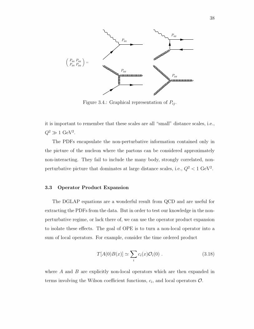
The meaning of each splitting function can be understood from Figure 3.4,

which illustrates that because the photon only couples to quarks, deep inelastic

electron scattering is only sensitive to the upper two diagrams. Ideally, a virtual

gluon probe, analogous to the virtual photon, would allow for a clean measure-

ment of the gluon distributions but it does not exist due to confinement. Instead

the Drell-Yan process (e.g. proton-proton collisions) can be used, in a limited

fashion, to probe the gluon distributions. Calculations of splitting functions can

be found in [34] and references therein.

3.2.3 PDFs

For nearly 30 years, experiments have extracted the PDFs from process that

include DIS, Drell-Yan, and SIDIS. The parton distributions are the same in all

processes and are therefore seen as universal. Figure 3.5 is one example of how

the DGLAP equations succeed at describing the data over a wide of scales, but

38

(

Pqq Pqg

Pgq Pgg

)

=

Pqq

Pqg

Pgg

Pgg

Figure 3.4.: Graphical representation of Pij.

it is important to remember that these scales are all “small” distance scales, i.e.,

Q2 ≫ 1 GeV2.

The PDFs encapsulate the non-perturbative information contained only in

the picture of the nucleon where the partons can be considered approximately

non-interacting. They fail to include the many body, strongly correlated, non-

perturbative picture that dominates at large distance scales, i.e., Q2 < 1 GeV2.

3.3 Operator Product Expansion

The DGLAP equations are a wonderful result from QCD and are useful for

extracting the PDFs from the data. But in order to test our knowledge in the non-

perturbative regime, or lack there of, we can use the operator product expansion

to isolate these effects. The goal of OPE is to turn a non-local operator into a

sum of local operators. For example, consider the time ordered product

T [A(0)B(x)] ≃∑

i

ci(x)Oi(0) . (3.18)

where A and B are explicitly non-local operators which are then expanded in

terms involving the Wilson coefficient functions, ci, and local operators O.

39

x

3−10 2−10 1−10 10

0.2

0.4

0.6

0.8

1

1.2

1.4

1.6

1.8

2OLDSLAC

NMC

JLAB-E94110

Stat. Model

OLDSLAC

EMC

ZEUS

BCDMS

NMC

2 = 90 GeV2Q

2 = 2 GeV2Q

Figure 3.5.: Data on the structure function F p2 along with the result calculated

from an evolved fit [35]. The fit is calculated at the mean value of Q2 for theselected data around Q2 = 2 GeV2 (black) and Q2 = 90 GeV2 (red).

The spin structure functions are related to the time ordered product appear-

ing in the forward part of the virtual Compton amplitude (see Appendix A). The

operators required in this expansion are characterized by isospin and twist. The

leading twist (τ = 2) operators are related to the parton distribution functions

and their coefficient functions are directly related to the splitting functions of

the DGLAP equations. For more details on the OPE see appendix B.

Revisiting the Ellis-Jaffe sum rule, and including the leading twist pQCD

corrections [36], it now has the form

∫ 1

0

dxgp1(x,Q2) = Cns(Q

2)

(

± 1

12g3(Q

2) +1

36a8(Q

2)

)

+ Cs(Q2)1

9∆Σ(Q2) + HT

(3.19)

where Cns and Cs are the non-singlet and the singlet coefficient functions re-

spectively. The HT represents the higher twist contributions to first moment of

40

g1. Note that there is now an explicit Q2 dependence in the moments of the

distributions implying a dependence on the gluon distribution.

3.3.1 Higher Twists

At large values of Q2 non-perturbative effects contribute but their size is

negligible. At lower Q2 their contribution becomes important. These show up

as corrections proportional to (1/Q2)n and involve quark-gluon correlations that

cannot be obtained in the naive parton model.

These non-perturbative corrections, referred to as higher twist or power cor-

rections, can be carefully extracted from experiment using the operator product

expansion beyond the leading-twist approximation. Often they can also be cal-

culated from phenomenological models or Lattice QCD. Comparisons of higher

twist corrections against Lattice QCD predictions provide fundamental tests of

non-perturbative QCD.

Within the so-called twist expansion the moment has the form

Γ1(Q2) =

∫ 1

0

dx g1(x,Q2) = µ2(Q

2) +µ4(Q

2)

Q2+µ6(Q

2)

Q4+ . . . (3.20)

where the leading twist term

µp,n2 = Cns(Q2)

(

± 1

12gA +

1

36a8

)

+ Cs(Q2)1

9∆Σ (3.21)

is just the sum rule in 3.19. The Q2 of µ2 is well understood and measured.

However, the higher twist contribution and their Q2 dependence is not well

understood or measured. It is clear from the twist expansion that at large Q2

the higher twist terms are suppressed. As experiments probe larger distances

there remains an important question to answer: At what scale do the higher

twist terms become important?

41

At this point it is worth introducing the explicit notation for the twist de-

composition of the spin structure functions

gexp1 (x,Q2) = gτ=21 (x,Q2) + gτ=3

1 (x,Q2) + . . .

gexp2 (x,Q2) = gτ=22 (x,Q2) + gτ=3

2 (x,Q2) + . . .(3.22)

where the gτ=21 should be substituted into 3.19 when neglecting the higher twist

terms.

It should be emphasized that the PDFs measured in deep inelastic scattering

only contribute to the leading twist part of the structure functions, and that at

lower Q2, where the precise onset of higher twists is unknown, extraction of the

leading twist alone can be problematic. That is, one should be careful not to

mix higher twists with renormalization scale effects.

3.3.2 Moments

From the OPE an infinite set of sum rules relating the proton matrix ele-

ments to the x moments of the structure functions. Neglecting quark mass and

target mass effects the reduced matrix elements (defined in Appendix B) can be

calculated from moments of g1 and g2,

∫ 1

0

dxxn−1 g1(x,Q2) =

1

2an−1(Q

2) n = 1, 3, 5 . . . (3.23)

and

∫ 1

0

dx xn−1g2(x,Q2) =

n− 1

2n

(

dn−1(Q2)− an−1(Q

2)

)

n = 3, 5, 7 . . . (3.24)

42

where an−1 are twist-2 and dn−1 are twist-3 reduced matrix elements. Noting

that 3.24 starts at n = 1, the OPE does not predict the Burkhardt-Cottingham

sum rule [37]∫ 1

0

dxg2(x,Q2) = 0. (3.25)

Experimentally the sum rule seems to hold but the data is not precise enough at

low x to very well constrain the result. It is interesting that should if equation 3.24

holds for n = 1 it would reduce to the BC sum rule.

Wandzura-Wilzcek Relation

Perhaps the closest analog to the Callan-Gross relation for the spin struc-

ture functions comes from the leading twist approximation of the moments in

equations 3.23 and 3.24 for n = 3. The Wandzura-Wilczek relation [38],

gWW2 (x) ≡ gτ=2

2 (x) = −gτ=21 (x) +

∫ 1

x

dy

ygτ=21 (y) (3.26)

relates the leading twist part of g1 to the leading twist part of g2. If the twist-3

contribution is included, the structure function g2 has an additional term

g2(x) = gWW2 (x) + g2(x) (3.27)

where the higher twist part is

∫ 1

0

dxxn−1gn−1(x) =n− 1

2ndn−1(Q

2) n = 3, 5, 7 . . . (3.28)

43

Blumlein-Tkabladze Relation

When considering target mass effects a relation [39] between the twist-3 part

of g2 shows up in g1 as the target mass correction

gτ=31 (x) =

4M2x2

Q2

[

gτ=32 (x)− 2

∫ 1

x

dy

ygτ=32 (y)

]

. (3.29)

As will soon be discussed, this target mass correction is responsible for the next-

to-leading appearance of d2 in the twist expansion of Γ1. This relation is as

important to consider as the Wandzura-Wilczek relation when trying to extract

higher twist decomposition of g2. A simultaneous separation of higher twists

from both g1 and g2 would be the ideal method in order to avoid including

spurious twist-3 contributions in gWW2 by neglecting equation 3.29. It has been

demonstrated [40] that making this mistake for the proton may end up causing

a sinister cancellation of gτ=32 .

3.4 Color Forces

The ground work laid out by the OPE allows for the extraction of interesting

physics from precision measurements of the spin structure functions. A measure-

ment of the g2 structure function is directly sensitive to quark gluon correlations

as shown in Figure 3.6b. In particular, the twist-3 matrix element can be extract

from the data via

d2(Q2) =

∫ 1

0

dxx2 (2g1(x) + 3g2(x)) . (3.30)

At largeQ2 where the d2 is proportional to an average transverse color Lorentz

force acting on the struck quark the instant after being struck by the virtual

photon [18,41]. This can be easily seen by explicitly writing the matrix element

d2 =1

2MP+2Sx〈P, S | q(0)gG+y(0)γ+q(0) | P, S〉. (3.31)

44

(a) (b) (c) (d)

Figure 3.6.: Diagrams for operators in the twist expansion.

Exploiting the fact that the proton is moving in the infinite momentum frame,

i.e., ~v = −cz, the field strength tensor becomes

[

~E + ~v × ~B]y

= Ey +Bx =√2G+y (3.32)

and

F y = −√2

2P+〈P, S

∣

∣q(0)G+y(0)γ+q(0)∣

∣P, S〉

= −2√2MP+Sxd2

= −2M2d2

(3.33)

It should be emphasized here that a measurement of g2 is directly sensitive

to an average color Lorentz force. This puts polarized DIS in an entirely unique

situation to begin precision measurements in QCD.

Furthermore, when considering higher twist matrix elements Burkardt [18]

showed that the color electric and magnetic forces can be separated by

FE =−M2

4

[

2

3(2d2 + f2)

]

(3.34)

FB =−M2

2

[

1

3(4d2 − f2)

]

. (3.35)

The twist-4 matrix element is defined as

f2 M2 Sµ =

1

2

∑

i

e2i 〈P, S| g ψi Gµνγν ψi |P, S〉

45

and it can be extracted from the first moment of g1. The next-to-leading twist

contribution to Γ1 is written in terms of the reduced matrix elements [42]

µ4 =M2

9

(

a2 + 4d2 + 4f2

)

, (3.36)

where a2 is twist-2, d2 is twist-3, and f2 is twist-4. Since µ4 does not enter at

leading twist it must determined by subtracting the, presumably well known,

leading twist

∆Γ1 = Γ1 − µ2 (3.37)

where the ∆Γ1 contains all higher twists. Therefore it should be clear that a

clean determination of f2 would require precision data taken at high Q2 in order

to make sure all higher twists are suppressed. Then by moving to lower Q2 the

with matched precision in d2 and a2 the difference can be attributed to f2 or even

higher twists. Before this can be done, however, the leading twist terms must be

well determined by precision measurements at low x, where the integral of the

first moment dominates, and large momentum transfers to ensure the absence of

higher twists.

3.4.1 Status of d2

So far the there have only been two measurements of dp2, although the first

is really an improved value by combining the results of SLAC E143, E155, and

E155x [43]. This result is at an average Q2 of 5 GeV2. The second measurement

was done by Resonance Spin Structure (RSS) experiment [44,45] which extracted

a value dp2 value at Q2 = 1.28 GeV2. These two results are shown in Figure 3.7

along with a lattice QCD calculation [46].

The elastic contribution to the integral at x = 1 can be calculated using

equations 2.34 – 2.37 and fits to the elastic form factors. Interestingly, when

46

)2 (GeV2Q

1 2 3 4 5 6 7 8 9 100.015−

0.01−

0.005−

0

0.005

0.01

0.015

0.02Lattice - Gockeler, et.al.

RSS

SLAC E155x+E155+E143

pQCD - Shuryak and Vainshtein

elastic

elastic + pQCD

Figure 3.7.: The world data on dp2 from SLAC [43] (open square) and RSS [45](filled square), and a lattice QCD calculation [46] (open circle).

form factors that include a two photon exchange correction are used, the elastic

contribution becomes slight negative around Q2 ∼ 3 GeV2.

3.5 Remarks

With the twist 3 matrix element and its physical interpretation, QCD is be-

ginning to enter the realm of tests through precision experiments. Confinement

does not permit us to measure color moments in the same way precision mag-

netic dipole moments are measured in QED. However, a d2 measurement is an

important step in moving our understanding of strong force into the precision

47

era. Just because it is small does not mean it is not important, e.g., the Lamb

shift was instrumental in the development of QED. A precision measurement of

d2 hopes to spur the development of ab initio QCD calculations.

48

49

CHAPTER 4

THE EXPERIMENT

The Spin Asymmetries of the Nucleon Experiment (E03-007) finished taking

data in March 2009 and the experiment took place in Hall C at Jefferson Lab.

Utilizing a polarized electron beam and a polarized proton target, two double

spin asymmetries were measured. The measured asymmetries are A180 and A80,

where the 180 (80) refers to α, the angle between the incoming beam and the

target polarization vector (see Figure 2.7). A large solid angle and momentum

acceptance detector package, the Big Electron Telescope Array (BETA), detected

scattered electrons in an open configuration at a scattering angle of 40 degrees.

The kinematic coverage of BETA is shown in Figure. 4.1. Although BETA

was fixed at 40 degrees, a large solid angle of about 200 mSr and large momentum

acceptance allowed for kinematics covering 0.3 < x <0.8 and 2.0 GeV2 < Q2 <

6.5 GeV2. The experiment used two beam energies, 4.7 GeV and 5.9 GeV.

We will begin this chapter by describing the accelerator and polarized electron

beam. The polarized target will be discussed in section 4.2, followed by an

overview of BETA in section 4.3.

4.1 Accelerator and Beamline

The Thomas Jefferson National Accelerator Facility operated a longitudinally

polarized electron beam capable of energies up to 6GeV . The continuous electron

beam accelerator facility (CEBAF), constructed in a “racetrack” configuration,

accelerates injected electrons along the straight sections. These straight sections

consist of multiple superconducting RF cavities through which electrons make

multiple passes, increasing the energy with each pass.

50

x

0.1 0.2 0.3 0.4 0.5 0.6 0.7 0.8 0.9 1

2 (

GeV

/c)

2Q

1

2

3

4

5

6

Figure 4.1.: Kinematic coverage of BETA for the two beam energies, 4.7 GeV(blue) and 5.9 GeV (red).

The polarized electron source begins with a cathode of strained GaAs. Al-

ternating circularly polarized light is produced by a Pockel Cell wich operates at

a frequency of about 30 Hz. The laser light ejects polarized electrons from the

cathode because the material is prepared, or strained, in order to lift the degen-

eracies that hamper high polarizations. Details of the injection system, design

and operation can be found in [47], [48], [49].

CEBAF is able to simultaneously provide beam to all three experimental

halls. However, the polarization at each hall is different and is dependent on

the number of passes (due to Larmor precession in the magnetic fields) and the

Wien filter angle used at the injector. Therefore, each hall measures the incoming

electron beam polarization independently.

51

Figure 4.2.: Overview of CEBAF reproduced from [47]

4.1.1 Hall C Beamline

Beam Energy Measurement

The beam energy is determined by measuring the position of the beam after

going through the well known arc magnets. The position is determined by using

superharps [50], which is a destructive measurement that scans the beam profile

with wires. The superharps can determine the position with a resolution of

roughly 10 µm at the entrance, midpoint, and exit of the arc [51]. The beam

energy is then calculated as

E ≃ e

θ

∫

Bdl (4.1)

where e is the electron charge, θ is the bend angle after traveling through the

arc, and the line integral is over the trajectory through the arc magnets with

known magnetic field B. As part of the Hall C standard beamline for more than

a decade [52], an accurate determination of the beam energy can be deduced

from the arc magnet current settings. These beam energies are shown Figure 4.3

for each run.

52

Run Number - 72000

100 200 300 400 500 600 700 800 900 1000

Bea

m E

ner

gy (

GeV

)

4

4.2

4.4

4.6

4.8

5

5.2

5.4

5.6

5.8

6

Figure 4.3.: Beam energies vs run number showing two beam energies, 4.7 GeVand 5.9 GeV.

Polarimeter

The Hall-C Møller polarimeter was used to measure the beam polarization

during the SANE to precision of less than a percent [53]. A disruptive measure-

ment, the Møller polarimeter measured the polarization a few times throughout

the experiment. The polarimeter consists of an iron target in a 4T magnetic

field, which predictably polarizes the target’s electrons. The scattering asymme-

try determines the beam polarization by using the Møller cross section equation

dσ

dΩ=

(

dσ0dΩ

)

[

1 + PbPtAzz(θ)]

(4.2)

where(

dσ0dΩ

)

is the unpolarized Møller cross section, Pb is the beam polarization,

Pt is the target electron polarization, and Azz is the so-called analyzing power,

which is a known function of the center of mass angle θ.

53

An effective electron target polarization of about 8% is achieved using a

pure iron target. The iron target sat upstream a few meters from a focusing

quadrupole, which is then followed by a collimation system which can be seen in

Figure 4.4. A defocussing quadrupole follows the collimator. A symmetric pair

of detectors consisting of a hodoscope and lead glass calorimeter measure the

coincident pair, a scattered electron and recoiling target electron.

Figure 4.4.: Layout of the hall-C Møller polarimeter. The top figure shows a closeup view of the collimation system and the bottom shows a larger view includingthe quadrupole magnet and electron detectors.

Beam Position Monitors

Two beam position monitors (BPM) were used to determine electron beam

position a locations upstream in the alcove and arc sections of the beamline.

Each BPM consists of a resonant cavity designed to match the accelerator beam

54

Run Number - 72000

200 300 400 500 600 700 800 900 1000

Pola

riza

tion (

%)

10

20

30

40

50

60

70

80

90

100

Figure 4.5.: Beam polarization vs run for the two helicities, positive (red) andnegative (blue).

pulse frequency at 1497 MHz, along with four antennae around the beam. These

antennae are rotated 45so that they are not damaged by synchrotron radiation

from the horizontal steering magnets. By measuring the phase locked signal

difference between opposite antennae, the relative position of the beam can be

determined.

Chicane and Helium Bag

A large magnetic field was required to operate the polarized target (see sec-

tion 4.2). For the longitudinal target polarizations this does not pose any ad-

ditional problems, however, for the transverse target configuration there was

significant beam deflection. An uncompensated beam therefore would not arrive

centered on the target. A chicane consisting of two dipoles was installed to posi-

55

tion the beam so that it arrives centered on the target with the same incidence

as the longitudinal target configuration.

Since a majority of the beam does not scatter or barely scatters at very small

angles and momentum transfers, the standard Hall C beam dump pipe needed

to be modified as well to accommodate the transverse field deflection. Just after

the target a large helium bag was installed with an extension arm to reach the

target vacuum chamber. This was needed to avoid activating the existing beam

pipe and limit contamination in the hall.

Beam Current Monitors

Two specially selected beam current monitors (BCMs) were used for the

experiment due to the relatively low beam current required for operating the

polarized target. These monitors were constructed from cylindrical resonant

cavities that matched the beam frequency in a non-destructive resonance mode.

The BCMs were calibrated against Faraday cup current measurements done at

the injector. The BCM outputs were fed to a voltage-to-frequency converter

which was then recorded by a scaler. Additionally, each BCM had a pair of

helicity gated scalers which only counted when the electron beam was of a given

helicity. These signals are determined by the sign of the voltage applied to the

Pockel cells at the accelerator injector.

Beam Raster

The beam is typically delivered with a spread on the order of 100 µm. This

very small size can induce local heating damage on the various windows and

targets of the beamline. Therefore, a fast raster system, consisting of two magnets

far upstream spreads the beam to an area of 2×2 mm2 [54]. The voltages across

these magnets were fed into the event data stream as ADC channels. These

provided access to the raster beam position event by event.

56

Similarly, the polarized ammonia target is currently limited and can expe-

rience large depolarizations due to the beam. In order to increase the running

luminosity, a slow raster was developed [55]. Unlike the fast raster, it rotated the

beam inward in a spiral pattern of 1 cm maximum radius, with a 30 Hz repetition

rate, matching both the beam pipe and target cell geometries. A diameter of

roughly 2 cm reduced the local heating load on the polarized target and allowed

for operation with beam currents near 100 nA.

4.2 Polarized Target

The experiment used polarized ammonia (NH3) as an effective polarized pro-

ton target. It was operated by the University of Virginia target group. The

target consisted of a superconducting magnet which produced a 5.1 T magnetic

field for polarizing the target material which is cooled to roughly 1K. Through

the technique of dynamic nuclear polarization (DNP) the target is capable of

achieving polarizations upwards of 90%, however, due to beam depolarization ef-

fects, the average polarization for this experiment was roughly 68%. The target

polarization for each run is shown in Figure 4.6.

Early on in the experiment the target magnet experienced a series of destruc-

tive quenches requiring serious repair [56]. The magnet troubles caused major

delay in experimental run time and severely limited the detector commission-

ing and calibration periods. Thanks to the efforts of the Hall C technicians and

target group the magnet was able to be repaired enough to finish the experiment.

The basic polarization mechanism is as follows. The strong magnetic field

causes a Zeeman splitting of the electronic (EPR) and nuclear (NMR) spins

leaving four possible configurations of the electron-proton spins. A spin-spin

interaction between the electron and proton spins allows for one of the double

spin flip transitions to be driven by saturating the target with microwaves. Then

by exploiting the roughly 4 orders of magnitude larger relaxation time of the

57

0%

20%

40%

60%

80%

100%

72100 72200 72300 72400 72500 72600 72700 72800 72900 73000 73100

Ab

so

lute

Po

lariza

tio

n

Run Number

Positive PolarizationNegative Polarization

Figure 4.6.: Target polarization by run number.

proton, the microwave frequency can chosen to drive the proton polarization

into either direction.

The polarization was determined by measuring the magnetic susceptibility

over a range of frequencies spanning the Larmor frequency for the proton. This

was accomplished by using a Q-meter to measure the frequency response of a coil

which surrounded the ammonia target material. This NMR coil drives the proton

into the metastable state, or if the microwaves are pumping the metastable state,

it stimulates photon emission to the stable state. These two states are referred

to as the positive and negative polarization states respectively.

An NMR resonance curve was obtained by sweeping the coil frequency, how-

ever, this signal was only proportional to the polarization. A thermal equilibrium

(TE) measurement was used to provide a proportionality constant needed to get

an absolute polarization from the NMR curves. By turning off the microwave

pumping, the polarization settles at the known thermal equilibrium value of

PTE = tanhµB

kT. (4.3)

58

The NMR curve at thermal equilibrium provided an absolute calibration for the

NMR system. The polarization while pumping is then calculated as

PDNP

PTE

=ADNP

ATE

GDNP

GTE

(4.4)

where ADNP and ATE are the areas under each NMR curve while pumping (DNP)

and while at thermal equilibrium (TE), and where G is the gain settings of the

amplifiers for each of the two measurements.

A drawing of the target system is shown in figure 4.7. The target used liquid

helium to cool both the magnet and the target cell.

Figure 4.7.: Drawing of the target vacuum chamber and magnet systems.

A more in depth description and analysis of the SANE polarized target can

be found in chapter 4 of James Maxwell’s thesis [56]. More details on general

design and operation of solid polarized targets can be found in [57], [58], and [59].

59

4.3 BETA

Cerenkov

Counter

Lucite

Hodoscope

BigCal

Forward

TrackerPolarized

Target

Target Outer

Vacuum

Chamber

Super

Conducting

Magnet

Figure 4.8.: BETA detectors with simulated event.

The Big Electron Telescope Array, BETA, was the primary detector package

for the experiment. It differed from traditional DIS experiments by making use of

a large acceptance electromagnetic calorimeter and detectors placed in an open

configuration where typically a magnetic spectrometer with a limited acceptance.

BETA comprises four detectors, a forward tracker placed as close to the target

as possible, followed by a threshold gas Cerenkov counter, a Lucite hodoscope

and a large electromagnetic calorimeter dubbed BigCal.

60

50 cm55 cm

61.5 cm

167 cm

2.53 m3.35 m45 cm

40 cm

122 cm

96 cm

120 cm122 cm

Figure 4.9.: BETA dimensions with side view (upper figure) and a top view(lower figure). Shown from left to right are the calorimeter, hodoscope, Cerenkovcounter, forward tracker and polarized target.

4.3.1 BigCal

THe BigCal electromagnetic calorimeter provided position and energy mea-

surements of the scattered electrons and photons. It consisted of 1744 lead glass

blocks and was divided into two sections.

The upper section (RCS) was from the Yerevan Physics Institute and was

previously used during the RCS experiment [60]. Consisting of 4×4×40 cm3 lead-

61

glass blocks, the RCS blocks were arranged in a 30× 24 array. The lower section

(Protvino) was from Institute for High Energy Physics in Protvino, Russia, and

it consists of 3.8× 3.8× 45 cm3 lead-glass blocks arranged in 32× 32 array.

Each block had a PMT and a corresponding ADC readout for each triggered

event. BigCal also was a primary component of the data acquisition triggers.

In order to reduce complexity and background through correlation a summation

scheme was implemented as shown in Figures 4.10 and 4.11. While each channel

had an ADC, the smallest segment to have a TDC were groups of 8 (sometimes

only 7 for RCS) blocks in the same row. These TDC groups, an example of which

is designated by the small hatched area in Figure 4.10, formed 4 timing columns

and were analog summed before a discriminated signal was fed to the TDC.

Protvino

RCS

Trigger GroupsT1 and T2

Trigger GroupsT3 and T4

A B C DTiming Columns

TDC Channel (A,5)

Timing Group 9

Figure 4.10.: BigCal timing groups and trigger summing scheme. Note thatsome blocks belong to more than one timing/trigger groups. See the text formore detail.

62

The analog sums of the TDC groups were split and then summed into larger

timing groups of 64 blocks, which span half the width of the detector and 4

blocks vertically. The timing groups were overlapped in order to avoid missing

a signal equally split between two groups and is illustrated by the alternating

colors shown in Figure 4.10, where an example is shown by the large hatched

area.

Finally, by summing the timing groups in each BigCal quadrant, four trigger

groups (T1, T2, T3, and T4) were constructed and used to form the main triggers

for the data acquisition. Due to the overlapping of the timing groups, one row

of blocks was shared between the RCS and Protvino trigger groups.

4.3.2 Gas Cerenkov

As can be seen in Figure 4.8, the front window of the Cerenkov counter was

positioned just behind the forward tracker while BigCal was set at roughly 3.5m

from the target. The dimensions and positions of the detectors and target are

shown in Figure 4.9.

The gas Cerenkov counter was designed and constructed at Temple Univer-

sity. It was filled with nitrogen gas at atmospheric pressure and used 4 spherical

and 4 toroidal mirrors to focus light to quartz window photomultiplier tubes.

These three inch quartz window tubes were selected for their UV transparency

which was complemented by the special mirror coating for high reflectivity far

into the UV. The photomultiplier tubes were aligned in a single column on the

side of the tank located at larger scattering angles (as shown in Figure 4.12) in

order to reduce the background rates.

Figure 4.13 shows the ADC spectra for each type of mirror. The Cerenkov

counter had a large signal of roughly 20 photo-electrons which allowed it to

identify the double track peak. This double track peak was instrumental in

removing a sizable background from pairs produced outside of the target. A

63

Pb glass blockPMT

× 224 TDC groups(8 blocks per group)

× 38 Timing groups(64 blocks per group)

× 4 Trigger groups

An

...

An+8

8∑

Sj8Disc TDC

Sj8

...

Sj+8

8

64∑

Disc TDCTj

64

Tj64

...

Tj+N64

N∑

Disc TDC

To Trigger Supervisor

Figure 4.11.: A simplified diagram of the BigCal electronics.

detailed discussion of the design and performance of the SANE Gas Cerenkov

can be found in [61].

4.3.3 Lucite Hodoscope

The Lucite hodoscope was built by the group at North Carolina A&T State

University. It consisted of 28 curved Lucite bars with light guides mounted to

edges cut at 45 as seen in Figure 4.14. Stacked vertically, each bar was 6 cm tall

and 3.5 cm thick and provided a vertical position measurement. Photomultipliers

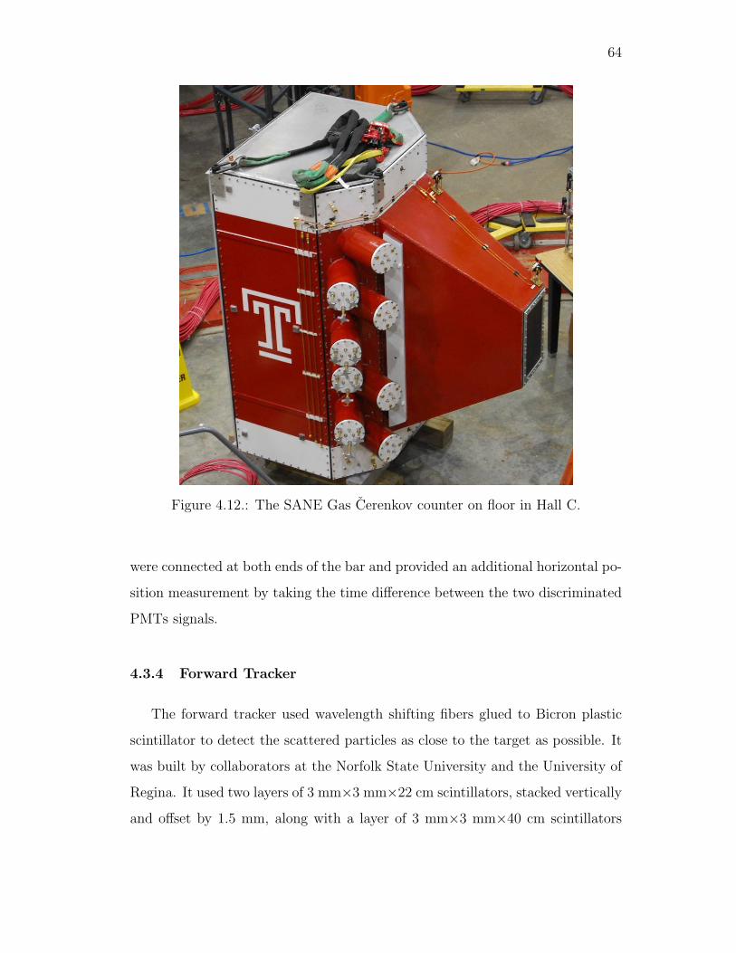
64

Figure 4.12.: The SANE Gas Cerenkov counter on floor in Hall C.

were connected at both ends of the bar and provided an additional horizontal po-

sition measurement by taking the time difference between the two discriminated

PMTs signals.

4.3.4 Forward Tracker

The forward tracker used wavelength shifting fibers glued to Bicron plastic

scintillator to detect the scattered particles as close to the target as possible. It

was built by collaborators at the Norfolk State University and the University of

Regina. It used two layers of 3 mm×3 mm×22 cm scintillators, stacked vertically

and offset by 1.5 mm, along with a layer of 3 mm×3 mm×40 cm scintillators

65

0 0.5 1 1.5 2 2.5 3 3.5 4

10

210

310

410

ADC0 0.5 1 1.5 2 2.5 3 3.5 4

1

10

210

310

Figure 4.13.: Cerenkov counter ADC spectrum for all the toroidal mirrors (top)and spherical mirrors (bottom).

grouped horizontally to provide a position measurement with a resolution suffi-

cient to distinguish between electron and positron trajectories of momenta, below

1 GeV/c. Due to a truncated commissioning period and higher than expected

background rates, the forward tracker was unable to cleanly separate by charge

the low energy pair symmetric background.

4.4 Data Acquisition

SANE used the CODA data acquisition system [62] to record event and slow

control data. It was controlled by the trigger supervisor (TS) which used a

distributed system of read out controllers (ROCs) that each ran a real-time

operating system on a single board computer. Typically each electronic crate had

a ROC. The event data consisted of all the detector ADC and TDC readouts.

66

Figure 4.14.: Photograph of three bars before mounting PMTs and wrapping.

67

Table 4.1.: SANE triggers defined for TS and their nominal prescale factors.

Name Prescale Description

PEDESTAL 1 Random gating of ADC for the first 1000events of each run.

BETA2 1 The main trigger requiring a Cerenkov andBigCal hit.

BETA1 9999 An alternate trigger between BigCal andCerenkov .

PI0 1 The π0 trigger requiring two BigCal quad-rants to have hits.

COIN 1 The coincidence trigger between BETA andthe HMS.

HMS1 1 HMS trigger for electronsHMS2 1 HMS trigger for hadrons

Many discriminator outputs were counted with scaler modules which provided

the important ability to measure the computer dead-time of the DAQ system.

The scalers were readout every two seconds. These “scaler events” were placed

in sync with the event data. The slow control data (EPICS [63]) was read out

every 2 and 30 seconds and was written to a separate data file.

The electronics for BETA were placed in the hall in concrete shielded hut,

while most of the (existing) HMS electronics are in the HMS hut or in the count-

ing house. A list of triggers for SANE are given in table 4.1 and a diagram of

the main triggers is shown in Figure 4.15.

68

Bigcal Trigger Group

Protvino RCS

T1 T2 T3 T4

Cerenkov Analog Sum

ACer1

...

ACer8

8∑

Disc

BETA2

PI0

Figure 4.15.: Definitions of the two main triggers, BETA2 and PI0.

69

CHAPTER 5

DATA ANALYSIS

This chapter describes each step in the detector analysis and the reconstruc-

tion of the physics events used to form the asymmetries. We begin with the

calorimeter clustering and calibration since it forms the starting point of any

track reconstructed by BETA. After the detector calibrations, the method of

event reconstruction and selection is presented. The chapter concludes with the

calculation of the measured asymmetries and the corrections need to arrive at

the asymmetries of physical interest.

5.1 Analysis Overview

The software for the analysis of BETA was written from scratch in C++

making use of the ROOT [64] libraries. The code developed is part of a new larger

library called InSANE [65]. The raw data recorded by CODA was extracted using

the Hall C ENGINE where the output HBOOK files were directly converted into

ROOT files. The scaler events were also incorporated into this new analysis code

base. A GEANT4 [66] simulation called BETAG4 [67] was developed as well.

One challenge was collecting and organizing the many disparate data sources

needed for the analysis. Therefore a run database, implemented in MySQL, was

the primary source for run information. This database was synchronized with a

run object stored in each ROOT file. The run object and database were updated

for each analysis pass described below.

The analysis was partitioned into a series of passes as outlined in table 5.1.

Each pass had a list of corrections and calculations that were performed at the

event level. All the corrections, e.g. ADC pedestal subtraction, were performed

70

before processing the calculations, e.g. converting an ADC value into an en-

ergy. This allowed for a systematic and incremental approach to constructing

the analysis.

At the scaler event level, each analysis pass contained a list of scaler cal-

culations and filters which were processed for each scaler event. Because the

scalers were synchronized with detector events, the filters performed calculations

for the interval of detector events by looking to the next scaler event. In a very

general way this allowed for data quality checks to be automatically performed

by raising flags or skipping bad periods of an otherwise good run. For example,

a beam current filter was written to monitor for beam current issues like beam

trips. Below a threshold of 70 nA, it raised a warning flag (which was recorded

in a run database), but when the beam current fell below 60 nA it recorded a

beam trip and skips the events between scaler reads until a proper beam current

is restored. The beam trip information (run number, starting time, duration,

threshold value) were also recorded in a run database.

5.2 Clustering

Clustering is a large field of data analysis and has many uses. For present

purposes we refer to clustering as partitional clustering, as opposed to a hierar-

chical clustering. For each event that triggers either the BETA2 or PI0 triggers, it

is likely that a shower spread across a few blocks and should be grouped into a

cluster. We must determine the number of clusters and determine which blocks

are associated with each cluster.

This may seem straightforward, however, operating in an open configuration

increases the amount of background and clustering should be done carefully to

avoid noisy blocks and overlapping showers.

71

Table 5.1.: An outline of tasks for each analysis pass.

Pass Description-2 • Raw data extracted

• HBOOK files converted into ROOT files.

• Epics data filled in a database.

-1 • Raw data ntuples converted into InSANE analysistrees.

• Scalers converted into InSANE scaler tree.

• Fits ADC pedestals

• Finds timing peaks

• Calorimeter clustering

0 • Subtracts ADC pedestals

• Performs time-walk corrections

• Calculates accumulated charge

• Calculates calibrated results (e.g. block energies,Cerenkov photoelectrons . . . )

1 • Performs hit position reconstruction

• Cluster correlations with other detectors

• Neural Network corrections

• Simple track reconstruction

2 • Detailed track reconstruction

• Vertex reconstruction

• Backward track propagation and tracking

72

5.2.1 Clustering Algorithm

There are variety of techniques for clustering which require the number of

clusters to be determined ahead of time. Determining the number of clusters

can be simple or complicated. For BigCal, we expected only a few clusters

per event, however, the maximum number of clusters was not fixed in order to

avoid missing events and to provide the possibility of rejecting events with too

many clusters. Initially, a k-means clustering algorithm was implemented but

this required a fixed number of clusters and it was computationally slow for our

purposes. Instead, a simple algorithm for determining the number of clusters

and associated blocks was developed as follows.

First, from a two dimensional histogram of the event, the calorimeter block

with the largest energy is selected as the cluster center. A 5 × 5 group of blocks

is formed around this centroid as shown in Figure 5.2a. If the blocks on the

perimeter of this group are detached, they are not included in the cluster. The

clusters shown in Figure 5.2 show some examples of clusters. Blocks with non-

zero energy that are included in the cluster are shown in red, while detached

blocks are shown in green.

E

Thresh.

Figure 5.1.: Diagram demonstrating the clustering energy threshold.

Once the detached blocks are removed from the cluster group, those blocks

remaining form a cluster and their values are set to zero in the search histogram.

Then the next highest energy block forms the seed of the next cluster and so on.

73

(a) (b) (c) (d) (e)

Figure 5.2.: Various classes of clusters. See text for details.

This continues until there are no more blocks with energy above a threshold (see

Figure 5.1) of roughly 400 MeV, at which point the search ends.

5.2.2 Cluster Characterization

Once the number of cluster centroids and their corresponding blocks have

been determined, various moments characterizing the cluster are calculated and

stored. They will be used as inputs for the artificial neural network corrections

in appendix C.

The first moment gives the cluster’s x and y position

µx =∑

i,j

xijEijET

µy =∑

i,j

yijEijET

(5.1)

where the total cluster energy is ET =∑

Eij, xij(yij) is the x(y) position of the

block (i,j) in BigCal column/row coordinates. The second moment gives the

standard deviations

σx =

√

∑

i,j

(xij − µx)2EijET

σy =

√

∑

i,j

(yij − µy)2EijET

(5.2)

74

which indicate the shower size and spread. The skewness is calculated as

γx1 =∑

i,j

(xij − µx)3EijET

γy1 =∑

i,j

(yij − µy)3EijET

(5.3)

which indicates the symmetry of the clusters profiles. A negative(positive) skew-

ness means it is leaning towards larger(smaller) values. The final statistical

measure used in characterizing a cluster is the kurtosis which gives a measure of

the peakedness. Specifically, we calculate the excess kurtosis as

γx2 =

(

∑

i,j

(xij − µx)4EijET

)

− 3

γy2 =

(

∑

i,j

(yij − µy)4EijET

)

− 3 .

(5.4)

5.3 Detector Calibrations

5.3.1 BigCal Energy Calibration

Unfortunately due to limited experimental beam time and problems with the

polarized target magnet, the planned elastic calibrations were not completed.

Therefore, the primary energy calibration was achieved through the technique of

reconstructing π0 decays.

Of the many backgrounds are the decay products of the π0 meson. Because

the decay channel is through the strong force (τ ∼ 10−27 s), the π0 decays

almost instantly. Therefore, we can safely assume the vertex for such a decay is

located at the target. The most probable decay channel is through two photons

with a branching ratio, Γγγ/Γtotal ≃ 0.99. The next highest decay channel is

π0 → e+e−γ with a branching ratio of approximately one percent.

75

/ ndf 2χ 6551 / 118

A 2.567e+03± 8.275e+05

Γ 0.1± 14.2

πM 0.0± 135.2

p0 9.3±1608 −

p1 0.20± 29.92

p2 0.0006±0.0619 −

GeVγ γM

0 50 100 150 200 250 300 350 400 450 5000

2

4

6

8

10

12

14

16

18

20

310× / ndf 2χ 6551 / 118

A 2.567e+03± 8.275e+05

Γ 0.1± 14.2

πM 0.0± 135.2

p0 9.3±1608 −

p1 0.20± 29.92

p2 0.0006±0.0619 −

mass0π

Figure 5.3.: A fit to the calibrated two photon invariant mass spectrum near theπ0 mass peak.

Two photons events were recorded by the PI0 trigger. After clustering, the

events were selected with an anti-Cerenkov cut on both clusters. The recon-

structed mass is

M2γγ = 2ν1ν2(1− cos(θγγ)) (5.5)

where ν1,2 are the photon energies and θγγ is the angle between them. The

resulting mass spectrum after calibrating is shown in Figure 5.3. More details of

the calibration method and procedure can be found in appendix D.

5.3.2 Gas Cerenkov

Number of Photoelectrons

During the experiment the gas Cerenkov high voltages were set to roughly

100 ADC channels per photo electron. The calibrated number of photoelectrons

76

for each PMT is shown in Figure 5.4. In order to provide a single variable for

event selection, the ADC peaks are aligned as shown in Figure 5.5.

0 10 20 30 40 50 0 10 20 30 40 50

0 10 20 30 40 50 0 10 20 30 40 50

0 10 20 30 40 50 0 10 20 30 40 50

photoelectrons0 10 20 30 40 50

photoelectrons0 10 20 30 40 50

Figure 5.4.: Number of photoelectrons for each Cerenkov mirror.

Cluster Position Correlation

In order to determine the appropriate geometry cuts to place on clusters in

BigCal, the Cerenkov mirror edges are found in the BigCal coordinate system

by looking at clusters which have multiple TDC hits. The outlines of the mirrors

become visible as shown in Figure 5.6. It is interesting that the size of the

Cerenkov cone can be roughly estimated from the edge resolution of these hits.

From these mirror edge locations, the appropriate Cerenkov ADC sum can

be calculated. For example if the clusters position is well within the center of a

mirror, only that mirror is associated for the ADC and TDC. If it falls near a

mirror edge, the primary mirror’s TDC is used and the ADCs of both mirrors

77

0 0.5 1 1.5 2 2.5 3 3.5 0 0.5 1 1.5 2 2.5 3 3.5

0 0.5 1 1.5 2 2.5 3 3.5 0 0.5 1 1.5 2 2.5 3 3.5

0 0.5 1 1.5 2 2.5 3 3.5 0 0.5 1 1.5 2 2.5 3 3.5

Aligned response0 0.5 1 1.5 2 2.5 3 3.5

Aligned response0 0.5 1 1.5 2 2.5 3 3.5

Figure 5.5.: ADC Aligned response for each Cerenkov mirror.

are summed. Similarly, for events in one of the central corners, all four mirrors

are summed.

5.3.3 Lucite Hodoscope Calibration

Lucite Position

The Lucite hodoscope did not have any ADC data during the experiment. A

multi-hit TDC gathered hits from PMTs mounted on both sides of each bar. In

order to determine both and x and y position, a TDC hit is required on both

sides of the same bar. The timing difference form can then be mapped to a

x-position in bigcal. From this and a survey of the detector position prior to the

experiment, we can calculate a position at the face of hodoscope.

The index of refraction for Lucite is nLucite = 1.495 and the maximum angle

of the Cherenkov light cone is cos−1(1/nLucite) = 48 degrees. Since the light

78

x (cm)-60 -40 -20 0 20 40 60

y (

cm)

-100

-50

0

50

100

Cherenkov Mirror EdgesCherenkov Mirror Edges

Figure 5.6.: A calibration of the mirror edges.

will propagate along the bar with reflections of about 45 degrees, a photon’s

path length to the PMT light gudie will be about√2 larger than the direct

length. Using this approximation and knowing that the Jlab F1TDC’s have a

time resolution of about 60 ps per channel, we can get the direct length from the

TDC value as

xluc = (TDC)(60ps)c√2nLucite

≃ (TDC)(0.8505cm

chan) (5.6)

79

Figure 5.7.: An example of a Lucite Hodoscope X position calibration. Note thefit function gives the BigCal x-cluster position (vertical axis) as a function of theLucite hodoscope bar TDC difference.

5.3.4 Forward Tracker Calibration

The forward tracker position reconstruction relied on accurate knowledge

of each scintillator’s position. This required detailed construction and survey

information.

5.4 Event Reconstruction and Selection

The values of the relevant physical quantities at the target where recon-

structed using a two step sequence of neutral networks. The primary reason for

a two step process was to separate two unrelated corrections: the cluster position

correction and the reconstruction of the scattering angles at the target.

The first network provided a position correction for the cluster due to varying

angles of incidence. It calculated a cluster position correction to determine the

80

Target Cell

BigCal

(xbcB ,p

bcB )

(xbcC ,p

bcC )

Forward Tracker

(xtracC ,p

tracC )

y-z plane

x-z plane

(xrast,yrast)

(xtargB

,ptargB

)(xtrac

B ,ptracB )

∆tracy

(xtargC

,ptargC

)

∆Y

∆X

Figure 5.8.: Definition of BETA tracking positions.

track crossing position at the front face of the calorimeter, the BigCal plane,

as shown in C.1. The improvement in the position resolution can be seen in

Figure C.5 where the red curve shows the improved position resolution over the

cluster position .

The second network provided corrections to the scattering angles that are

naively calculated as straight lines from the target to the BigCal plane. It cor-

rected for the bending of the tracks as it transitioned through the target volume

of strong magnetic fields. This was also checked with two independent par-

ticle tracking codes. A detailed discussion of the neural networks is given in

appendix C.

The Cerenkov counter identified scattered electrons in coincidence with a

shower in BigCal. In order to reduce uncorrelated background, a timing cut was

placed on the TDC spectrum as shown in Figure 5.10. In order to reduce the

number of background events falling into this cut, the TDC peak was time-walk

corrected. As the red curve shows, this correction was small due to the large

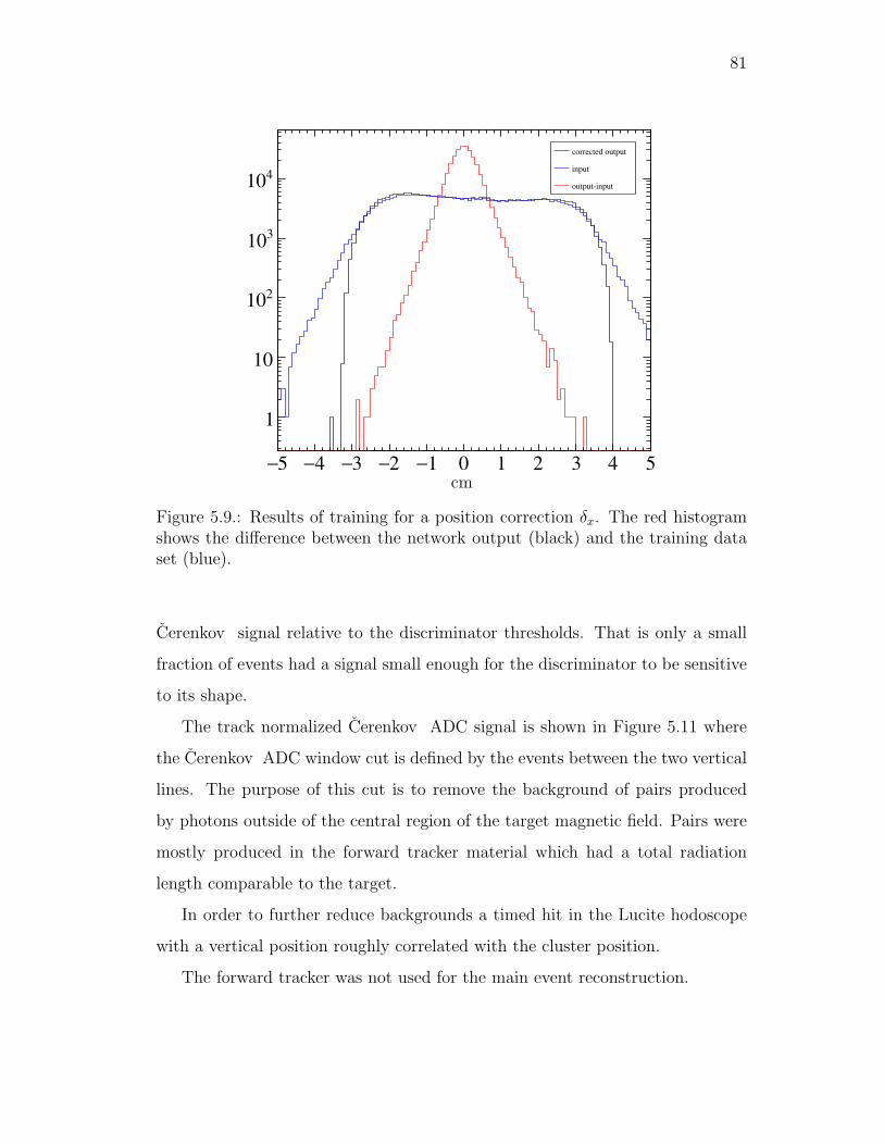
81

5− 4− 3− 2− 1− 0 1 2 3 4 5

1

10

210

310

410

corrected output

input

output-input

cm

Figure 5.9.: Results of training for a position correction δx. The red histogramshows the difference between the network output (black) and the training dataset (blue).

Cerenkov signal relative to the discriminator thresholds. That is only a small

fraction of events had a signal small enough for the discriminator to be sensitive

to its shape.

The track normalized Cerenkov ADC signal is shown in Figure 5.11 where

the Cerenkov ADC window cut is defined by the events between the two vertical

lines. The purpose of this cut is to remove the background of pairs produced

by photons outside of the central region of the target magnetic field. Pairs were

mostly produced in the forward tracker material which had a total radiation

length comparable to the target.

In order to further reduce backgrounds a timed hit in the Lucite hodoscope

with a vertical position roughly correlated with the cluster position.

The forward tracker was not used for the main event reconstruction.

82

TDC channel

50− 40− 30− 20− 10− 0 10 20 30 40 500

50

100

150

200

250

300

350

400

450

310×

Figure 5.10.: The Cerenkov TDC peak without (black) and with (red) a time-walk correction. The Vertical lines define the TDC selection cut.

5.5 Asymmetry Measurements

SANE set out to measured the double spin cross section asymmetry formed

by a polarized target and longitudinally polarized electron beam for two target

configurations. The two measured asymmetries utilized a target polarization

anti-parallel to the beam and a target polarization angle at 80 degrees. These

asymmetries, A80 and A180, are used to extract the proton’s virtual Compton

scattering asymmetries and spin structure functions.

The raw asymmetries must be corrected for a number of effects in order to ar-

rive at the asymmetries one would measure under ideal experimental conditions.

The ideal conditions would be a 100% polarized beam of nearly infinite current,

an infinitely thin target made of a single layer of protons with 100% polarization,

event selection cuts that provide 100% background rejection efficiency, zero win-

dow and detector material thicknesses precluding external radiative corrections,

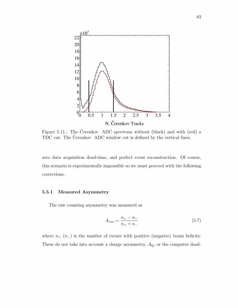
83

erenkov TracksCN.

0 0.5 1 1.5 2 2.5 3 3.5 40

2

4

6

8

10

12

14

16

18

20

22

310×

Figure 5.11.: The Cerenkov ADC spectrum without (black) and with (red) aTDC cut. The Cerenkov ADC window cut is defined by the vertical lines.

zero data acquisition dead-time, and perfect event reconstruction. Of course,

this scenario is experimentally impossible so we must proceed with the following

corrections.

5.5.1 Measured Asymmetry

The raw counting asymmetry was measured as

Araw =n+ − n−

n+ + n−

(5.7)

where n+ (n−) is the number of events with positive (negative) beam helicity.

These do not take into account a charge asymmetry, AQ, or the computer dead-

84

TDC channel

200− 150− 100− 50− 0 50 100 150 2000

500

1000

1500

2000

2500

3000

3500

Figure 5.12.: The Lucite Hodoscope TDC spectrum without (black) and with(red) the Cerenkov TDC cut.

time. Instead of using the raw event counts, n, the charge and live-time corrected

counts were used. The measured asymmetry becomes

Am =N+ −N−

N+ +N−

(5.8)

where the corrected rates are

N± =n±

Q±L±

, (5.9)

n± is the raw number of counts, Q± is the accumulated charge for the given

beam helicity over the counting period, and L± is the live time for each helicity.

The charge asymmetry used for each run is shown in Figure 5.13.

85

Run Number - 72000

400 500 600 700 800 900 10002−

1.5−

1−

0.5−

0

0.5

1

1.5

23−10×

Figure 5.13.: The charge asymmetry vs run number.

Live Time

The live time is the fraction of time that the data acquisition is available for

triggers and is related to the dead-time, L = 1−D, where L is the live time and

D is the dead time. The live time for each helicity was measured by the ratio of

triggers to scalers, L± = n±/s±. In this way the total counts for each helicity

can be properly corrected if the live time asymmetry is large.

The BETA DAQ had only the positive helicity input trigger scaler due to a

cabling problem. The live time was then calculated from a fit to the live time vs

the number of triggers between scaler readouts. This assumes that the live times

are proportional to the number of recorded triggers.

86

5.5.2 Corrected Asymmetry

The asymmetry is calculated as

Aphysics =1

df(W,Q2)PBPT

(

N+ −N−

N+ +N−

)

(5.10)

where PB and PT are the beam and target polarizations which have been previ-

ously calculated in sections 4.1.1 and 4.2. The dilution factor, df(W,Q2), takes

into account scattering from unpolarized nucleons in the target.

Figure 5.14.: Asymmetries after correcting for beam polarization, target polar-ization, and target dilution. The top plots show the anti-parallel configurationand the bottom show the perpendicular.

87

5.5.3 Dilution factor

The dilution factor was calculated for each run following

df(W,Q2) =Npσp(W,Q

2)

Npσp(W,Q2) +∑

iNiσi(W,Q2)(5.11)

where Np is the number density of protons (in NH3) and Ni is the density of

all the other nuclei that make up the target. This includes contributions from

the entrance and exit windows, liquid helium, NMR coil. All materials used to

calculate the dilution can be found in table C.1 of [56].

The polarized target material was formed into solid ammonia beaks and

placed into a cup which was inserted into a bath of liquid helium. In order

to determine the number density of polarized proton, the so called packing frac-

tion is the ratio of bead material to liquid helium found within the volume of

the target cell (see Figure 5.15).

The packing fraction were determined by comparing the yields measured by

the High Momentum Spectrometer (HMS) to a simulation. A carbon target with

an precisely known packing fraction was used to provide a baseline and calibration

point for the simulation. For this reason carbon target runs were take throughout

the experiment in order to eliminate possible systematic variations in the HMS

yields over long periods of time. The packing fractions on average were around

60% and a detailed listing of each target cell load can found in Table 5.1 of [56].

e− beam

Ammonia beads

Liquid 4He

∼ 3 cm

Figure 5.15.: A diagram of the target cup showing the packing fraction.

88

The cross sections in 5.11 were calculated from empirical fits to the structure

functions and form factors. The cross sections included all radiative corrections

calculated in appendix E. Their accurate calculation was instrumental in pushing

the energy cut lower where the elastic and quasi-elastic radiative tails become

significant. The growing contribution from the proton elastic radiative tail can

be seen in the dilution factor shown in Figure 5.16.

x

0.1 0.2 0.3 0.4 0.5 0.6 0.7 0.8 0.90

0.05

0.1

0.15

0.2

0.25

0.3

Figure 5.16.: The dilution factor calucated for run 72925 as a function of x,showing the increasing contribution from the elastic tails at lower energies (i.e.lower x).

5.6 Pair Symmetric Background

After correcting for polarization and target dilution, the background of positrons,

almost entirely due to π0 decays, was corrected for with a background dilution

89

term and a contamination term which was subtracted. The correction can be

written

Acor = CpairAphys (5.12)

=

(

1

fbg

)

Aphys −(

CAbg

)

(5.13)

where Cbg is a contamination due the asymmetry of the pair symmetric back-

ground and fbg is a background dilution. The resulting asymmetry, Acor, is the

asymmetry after correcting for the background a is now only due to scattered

electrons.

A fit of inclusive charged pion asymmetries was performed by Oscar Rondon

[68] in order to estimate the size of the contamination term in 5.12. It was

determined that for SANE the background asymmetry is Abg ≃ −0.022± 0.002.

x

0.2 0.3 0.4 0.5 0.6 0.7 0.8 0.91

1.05

1.1

1.15

1.2

1.25

1.3

1.35

1.4 2=1.6 GeV⟩

2Q⟨

2=2.9 GeV⟩

2Q⟨

2=4.1 GeV⟩

2Q⟨

2=6.1 GeV⟩

2Q⟨

x

0.2 0.3 0.4 0.5 0.6 0.7 0.8 0.90.02−

0.015−

0.01−

0.005−

0

0.005

0.01

0.015

0.022

=1.6 GeV⟩2

Q⟨2

=2.9 GeV⟩2

Q⟨2

=4.1 GeV⟩2

Q⟨2

=6.1 GeV⟩2

Q⟨

Figure 5.17.: The background dilution (left), 1/fbg, and background contamina-tion (right), Cbg, terms calculated for the anti-parallel 5.9 GeV configuration.

5.7 Radiative Corrections

After correcting for the pair symmetric background the radiative corrections

were applied following the standard formalism laid out by Mo and Tsai [69] as

90

Figure 5.18.: Same as Figure 5.14 but with the asymmetries corrected for thepair symmetric background.

well as the polarization dependent treatment of Akushevich, et.al. [70]. Many

details of the radiative corrections can be found in appendix E.

The elastic radiative tail was calculated from models of the proton form factor

[71] and a detailed description of the target geometry. The asymmetry was

corrected with an elastic dilution factor and contamination term. The total

“radiated” asymmetry (corrected for pair symmetric background) is

Acor =∆Tr+t

ΣTr+t

=∆inr+t +∆el

r+t

Σinr+t + Σel

r+t

(5.14)

91

where ∆r+t is the difference between radiated cross sections, and Σr+t is the

cross section sum. The superscripts indicate the total, inelastic, and elastic cross

sections should be used, respectively.

We are interested in obtaining the inelastic Born cross section asymmetry,

Ain0 , and therefore must subtract the elastic tail contributions. Using 5.14, this

asymmetry is

Ain =∆inr+t

Σinr+t

=1

felAcor − Cel

(5.15)

where1

fel=

ΣTr+t

Σinr+t

(5.16)

and

Cel =∆elr+t

Σinr+t

. (5.17)

It is clear from 5.16 and 5.17 that not only an accurate calculation of the elastic

radiative tail is needed to subtract the elastic tail, but an accurate calculation

of the inelastic radiative tail as well.

The dilution and contamination terms are shown in Figure 5.19. As expected

the dilution term follows the shape of the elastic radiative tail (see E.1).

Typically after subtracting the elastic tail contributions the Born cross sec-

tion is obtained by fitting the data in an iterative fashion. This assumes that

there is a wide range of kinematics covered in scattered energy and incident

energy as discussed in appendix E. Furthermore, since only an asymmetry was

measured over limited kinematics an unfolding procedure becomes impossible.

The correction to the asymmetry is calculated as a contamination

Ain0 = Ain − Cin. (5.18)

92

x

0 0.1 0.2 0.3 0.4 0.5 0.6 0.7 0.8 0.9 11

1.1

1.2

1.3

1.4

1.5

1.6

1.7

1.8

1.9

2

x

0 0.1 0.2 0.3 0.4 0.5 0.6 0.7 0.8 0.9 1

0.2−

0

0.2

0.4

0.6

0.8

1

Figure 5.19.: Elastic radiative tail dilution 1/fel (left), and contamination Cel(right) calculated for the parallel (black) and perpendicular (red) configurationsfor a 4.7 GeV incident beam energy.

Fortunately the correction for the inelastic radiative tail calculated from dif-

ferent models and fits is small. Using a variety of input models to understand

the systematic error introduced, the inealstic

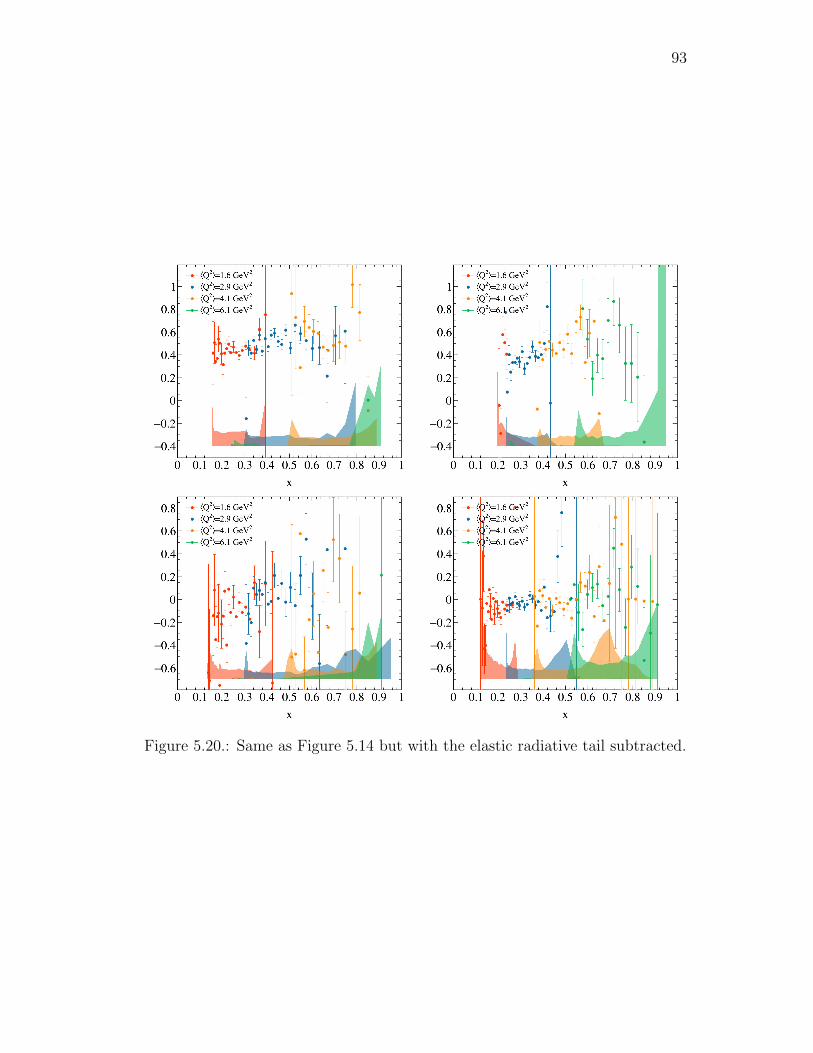
93

Figure 5.20.: Same as Figure 5.14 but with the elastic radiative tail subtracted.

94

W

1 1.5 2 2.5 3 3.5

(n

b/G

eV/s

r)Ω

/dE

d180

σd

3−10

2−10

1−10

1

10

Figure 5.21.: The inelastic radiative tail (blue), elastic radiative tail (red), andinelastic Born (black) cross sections for the anti-parallel target configurationand 5.9 GeV incident beam energy. The dashed lines are the cross sectionscorresponding to the two beam helicity states.

95

W

1 1.5 2 2.5 3 3.5

180

A

0

0.1

0.2

0.3

0.4

0.5

0.6

0.7

0.8

0.9

1

Figure 5.22.: The inelastic radiative tail (blue), elastic radiative tail (red), andinelastic Born (black) cross sections for the anti-parallel target configurationand 5.9 GeV incident beam energy. The dashed lines are the cross sectionscorresponding to the two beam helicity states.

96

Figure 5.23.: Same as Figure 5.14 but with the inelastic radiative tail corrected.

97

CHAPTER 6

RESULTS

The final results of the experiment are presented here. Tables of results can be

found appendix H. We begin by presenting the results for the virtual Compton

asymmetries because they have the least model dependence in their extraction.

The results of A1 are compared to the world data, models, and predictions for

high x. Then we will present the results for the spin structure functions g1 and

g2. From the these results the dynamical twist-3 matrix element is determined.

We will conclude with a discussion of the average color forces.

6.1 Virtual Compton Scattering Asymmetries

The corrected asymmetries found in Figure 5.23 are used to calculate A1

and A2 following equations A.20 and A.20. The SANE results are shown Fig-

ure against the world data for 8 > Q2 > 1 GeV2.

The behavior of Ap1 as x → 1 is particularly interesting because there are a

variety of model predictions. A recent calculation using the Dyson-Schwinger

equation approach [72] provides a new and interesting test in addition to those

of [73–76].

6.2 Spin Structure Functions

The spin structure functions were determined using equations A.16 and A.17

where an empirical fit was used for calculating F1 [85, 86].

98

W (GeV)

1 1.2 1.4 1.6 1.8 2 2.2 2.4 2.6 2.8 3 3.2 3.40

0.1

0.2

0.3

0.4

0.5

0.6

0.7

0.8

0.9

1

SLAC E143

SLAC E155

SMC

CLAS-E93009

HERMES

SANE

Figure 6.1.: The results for Ap1. The data [77–82] shown is limited to the range8 > Q2 > 1 GeV2.

W (GeV)

1 1.2 1.4 1.6 1.8 2 2.2 2.4 2.6 2.8 3 3.2 3.4

0.6−

0.4−

0.2−

0

0.2

0.4

0.6

0.8

SLAC E143

SLAC E155

SLAC E155x

SMC

HERMES

SANE

Figure 6.2.: The results for Ap2. The data [43, 78, 80, 83, 84] shown is limited tothe range 8 > Q2 > 1 GeV2.

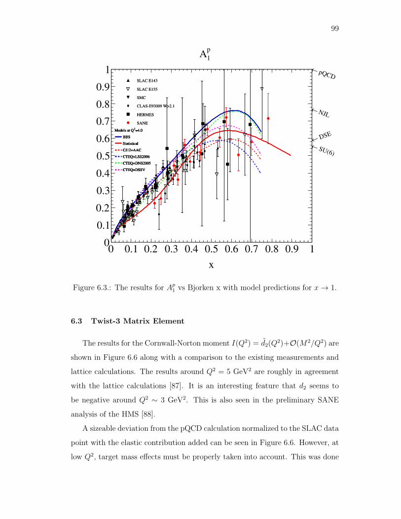
99

x

0 0.1 0.2 0.3 0.4 0.5 0.6 0.7 0.8 0.9 10

0.1

0.2

0.3

0.4

0.5

0.6

0.7

0.8

0.9

1

p

1A

SLAC E143

SLAC E155

SMC

CLAS-E93009 W>2.1

HERMES

SANE

DSE←

SU(6)←

NJL←

pQCD←

=4.02

Models at Q

BBS

Statistical

CJ12+AAC

CTEQ+LSS2006

CTEQ+DNS2005

CTEQ+DSSV

=4.02

Models at Q

BBS

Statistical

CJ12+AAC

CTEQ+LSS2006

CTEQ+DNS2005

CTEQ+DSSV

=4.02

Models at Q

BBS

Statistical

CJ12+AAC

CTEQ+LSS2006

CTEQ+DNS2005

CTEQ+DSSV

SLAC E143

SLAC E155

SMC

CLAS-E93009 W>2.1

HERMES

SANE

=4.02

Models at Q

BBS

Statistical

CJ12+AAC

CTEQ+LSS2006

CTEQ+DNS2005

CTEQ+DSSV

Figure 6.3.: The results for Ap1 vs Bjorken x with model predictions for x→ 1.

6.3 Twist-3 Matrix Element

The results for the Cornwall-Norton moment I(Q2) = d2(Q2)+O(M2/Q2) are

shown in Figure 6.6 along with a comparison to the existing measurements and

lattice calculations. The results around Q2 = 5 GeV2 are roughly in agreement

with the lattice calculations [87]. It is an interesting feature that d2 seems to

be negative around Q2 ∼ 3 GeV2. This is also seen in the preliminary SANE

analysis of the HMS [88].

A sizeable deviation from the pQCD calculation normalized to the SLAC data

point with the elastic contribution added can be seen in Figure 6.6. However, at

low Q2, target mass effects must be properly taken into account. This was done

100

x

0 0.1 0.2 0.3 0.4 0.5 0.6 0.7 0.8 0.9 1

0.02−

0

0.02

0.04

0.06

0.08SLAC E143

SLAC E155

EMC

SMC

HERMES

COMPASS

CLAS

2=1.6 GeV⟩

2Q⟨

2=2.9 GeV⟩

2Q⟨

2=4.1 GeV⟩

2Q⟨

2=6.1 GeV⟩

2Q⟨

Stat 2015

BB

LSS2006

DSSV

Figure 6.4.: The results for x2gp1.

by using Nachtmann moments (see appendix B.2.1). The Nactmann moment

extraction of d2(Q2) = 2M3

2 (Q2) is shown in Figure 6.7. While the improvement

is consistent with numerical estimates of [89], there remains a notable difference

that is consistent with a negative or zero value around Q2 = 3.0 GeV2.

The statistical errors for the measured regions were conservatively calculated

by summing the errors in quadrature. The unmeasured regions at low and high x

were calculated from models. The uncertainties from these regions were added to

the systematic uncertainty. Finally, the elastic contribution at x = 1 is calculated

from models. It is rather model independent, but it worth noting that using the

usual dipole form factors leads to an elastic contribution that remains positive for

all Q2, while using empirical fits that include a two photon exchange correction

[71] leads to a very slight negative value around Q2 ∼ 3.5 GeV2.

101

x

0 0.1 0.2 0.3 0.4 0.5 0.6 0.7 0.8 0.9 10.1−

0.05−

0

0.05

0.1

0.15SLAC E143

SLAC E155

SLAC E155x

SMC

HERMES

2=1.6 GeV⟩

2Q⟨

2=2.9 GeV⟩

2Q⟨

2=4.1 GeV⟩

2Q⟨

2=6.1 GeV⟩

2Q⟨

Stat 2015

BB

LSS2006

DSSV

Figure 6.5.: The results for x2gp2.

)2 (GeV2Q

1 2 3 4 5 6 7 8 9 10

0.01−

0

0.01

0.02

0.03

0.04Lattice - Gockeler, et.al.

RSS

SLAC E155x+E155+E143

BETA2

d

HMS2

d

pQCD - Shuryak and Vainshtein

elastic

elastic + pQCD

Figure 6.6.: The results for the CN moment extraction of dp2 = I(Q2).

102

)2 (GeV2Q

1 2 3 4 5 6 7 8 9 100.015−

0.01−

0.005−

0

0.005

0.01

0.015

0.02Lattice - Gockeler, et.al.

RSS

SLAC E155x+E155+E143

pQCD - Shuryak and Vainshtein

elastic

elastic + pQCD

Figure 6.7.: The results of a Nachtmann moment extraction of dp2 = 2M32 shown

against the existing data. [43, 44, 90]

103

CHAPTER 7

RECOMMENDATIONS

Precision measurements of d2 on both the proton and neutron have the unique

opportunity to study QCD confinement and color forces. However, there is a

lack of high Q2 data for g1 and g2 at high x. With the JLab 12 GeV program

beginning, it is crucial that precision measurements, with both longitudinal and

transverse target polarization, are conducted to map out the valence kinemat-

ics. A future electron-ion collider will also provide a great improvement at low

x. Improving the quality of the low x data in the spin structure functinos is

important for managing the uncertainties of the first moments. This will enable

a better separation of the average chromo electric and magnetic forces.

Lattice QCD calculations of d2 have been neglected in recent years. Precise

predictions of the Q2 dependence of d2 can provide a straightforward test of

QCD.

104

REFERENCES CITED

[1] E. Rutherford. The scattering of alpha and beta particles by matter andthe structure of the atom. Phil.Mag., 21:669–688, 1911.

[2] J. Chadwick. Possible Existence of a Neutron. Nature, 129:312, 1932.

[3] Luis W. Alvarez and F. Bloch. A Quantitative Determination of the Neu-tron Moment in Absolute Nuclear Magnetons. Phys.Rev., 57:111–122, 1940.

[4] Robert Hofstadter. Electron scattering and nuclear structure.Rev.Mod.Phys., 28:214–254, 1956.

[5] Murray Gell-Mann and Yuval Neemam. The Eightfold way: a review witha collection of reprints. 1964.

[6] Richard E. Taylor. Inelastic electron - proton scattering in the deep con-tinuum region. Conf.Proc., C690914:251–260, 1969.

[7] Elliott D. Bloom, D.H. Coward, H.C. DeStaebler, J. Drees, Guthrie Miller,et al. High-Energy Inelastic e p Scattering at 6-Degrees and 10-Degrees.Phys.Rev.Lett., 23:930–934, 1969.

[8] Richard E. Taylor. Deep inelastic scattering: The Early years.Rev.Mod.Phys., 63:573–595, 1991.

[9] Henry W. Kendall. Deep inelastic scattering: Experiments on the protonand the observation. Rev.Mod.Phys., 63:597–614, 1991.

[10] Jerome I. Friedman. Deep inelastic scattering: Comparisons with the quarkmodel. Rev.Mod.Phys., 63:615–629, 1991.

[11] G. Zweig. An SU(3) model for strong interaction symmetry and its break-ing. Version 1. 1964.

[12] O.W. Greenberg. Spin and Unitary Spin Independence in a ParaquarkModel of Baryons and Mesons. Phys.Rev.Lett., 13:598–602, 1964.

[13] H. Fritzsch, Murray Gell-Mann, and H. Leutwyler. Advantages of the ColorOctet Gluon Picture. Phys.Lett., B47:365–368, 1973.

[14] David J. Gross and Frank Wilczek. Ultraviolet Behavior of NonabelianGauge Theories. Phys.Rev.Lett., 30:1343–1346, 1973.

[15] Jr. Callan, Curtis G. and David J. Gross. High-energy electroproductionand the constitution of the electric current. Phys.Rev.Lett., 22:156–159,1969.

105

[16] R.P. Feynman. The behavior of hadron collisions at extreme energies.Conf.Proc., C690905:237–258, 1969.

[17] Richard P. Feynman. Very high-energy collisions of hadrons.Phys.Rev.Lett., 23:1415–1417, 1969.

[18] Matthias Burkardt. The g(2) Structure Function. AIP Conf.Proc.,1155:26–34, 2009.

[19] A. Accardi, J.L. Albacete, M. Anselmino, N. Armesto, E.C. Aschenauer,et al. Electron Ion Collider: The Next QCD Frontier - Understanding theglue that binds us all. 2012.

[20] N. F. Mott and H. S. W. Massey. Theory of Atomic Collisions. Oxford,1965.

[21] M.N. Rosenbluth. High Energy Elastic Scattering of Electrons on Protons.Phys.Rev., 79:615–619, 1950.

[22] K.A. Olive et al. Review of Particle Physics. Chin.Phys., C38:090001,2014.

[23] M. Anselmino, A. Efremov, and E. Leader. The Theory and phenomenol-ogy of polarized deep inelastic scattering. Phys.Rept., 261:1–124, 1995.

[24] J.D. Bjorken and Emmanuel A. Paschos. Inelastic Electron Proton andgamma Proton Scattering, and the Structure of the Nucleon. Phys.Rev.,185:1975–1982, 1969.

[25] John R. Ellis and Robert L. Jaffe. A Sum Rule for Deep Inelastic Electro-production from Polarized Protons. Phys.Rev., D9:1444, 1974.

[26] J. Ashman et al. A Measurement of the Spin Asymmetry and Deter-mination of the Structure Function g(1) in Deep Inelastic Muon-ProtonScattering. Phys.Lett., B206:364, 1988.

[27] Elliot Leader and Mauro Anselmino. A Crisis in the Parton Model: Where,Oh Where Is the Proton’s Spin? Z.Phys., C41:239, 1988.

[28] J.D. Bjorken. Applications of the Chiral U(6) x (6) Algebra of CurrentDensities. Phys.Rev., 148:1467–1478, 1966.

[29] J.D. Bjorken. Inelastic Scattering of Polarized Leptons from PolarizedNucleons. Phys.Rev., D1:1376–1379, 1970.

[30] V.N. Gribov and L.N. Lipatov. Deep inelastic e p scattering in perturbationtheory. Sov.J.Nucl.Phys., 15:438–450, 1972.

[31] Guido Altarelli and G. Parisi. Asymptotic Freedom in Parton Language.Nucl.Phys., B126:298, 1977.

[32] Yuri L. Dokshitzer. Calculation of the Structure Functions for Deep Inelas-tic Scattering and e+ e- Annihilation by Perturbation Theory in QuantumChromodynamics. Sov.Phys.JETP, 46:641–653, 1977.

106

[33] F. Halzen and Alan D. Martin. QUARKS AND LEPTONS: AN INTRO-DUCTORY COURSE IN MODERN PARTICLE PHYSICS. 1984.

[34] Johannes Blumlein. The Theory of Deeply Inelastic Scattering.Prog.Part.Nucl.Phys., 69:28–84, 2013.

[35] Claude Bourrely and Jacques Soffer. New developments in the statisticalapproach of parton distributions: tests and predictions up to LHC energies.2015.

[36] S.A. Larin, Paulo Nogueira, T. van Ritbergen, and J.A.M. Vermaseren.The Three loop QCD calculation of the moments of deep inelastic structurefunctions. Nucl.Phys., B492:338–378, 1997.

[37] Hugh Burkhardt and W.N. Cottingham. Sum rules for forward virtualCompton scattering. Annals Phys., 56:453–463, 1970.

[38] S. Wandzura and Frank Wilczek. Sum Rules for Spin Dependent Electro-production: Test of Relativistic Constituent Quarks. Phys.Lett., B72:195,1977.

[39] Johannes Blumlein and Avtandil Tkabladze. Target mass corrections forpolarized structure functions and new sum rules. Nucl.Phys., B553:427–464, 1999.

[40] Alberto Accardi, Alessandro Bacchetta, W. Melnitchouk, and MarcSchlegel. What can break the Wandzura-Wilczek relation? JHEP,0911:093, 2009.

[41] Matthias Burkardt. Transverse Structure of Hadrons. pages 101–110, 2010.

[42] Xiang-Dong Ji and W. Melnitchouk. Spin dependent twist four matrixelements from g1 data in the resonance region. Phys.Rev., D56:1–5, 1997.

[43] P.L. Anthony et al. Precision measurement of the proton and deuteronspin structure functions g(2) and asymmetries A(2). Phys.Lett., B553:18–24, 2003.

[44] Frank R. Wesselmann et al. Proton spin structure in the resonance region.Phys.Rev.Lett., 98:132003, 2007.

[45] K. Slifer et al. Probing Quark-Gluon Interactions with Transverse PolarizedScattering. Phys.Rev.Lett., 105:101601, 2010.

[46] M. Gockeler, R. Horsley, D. Pleiter, Paul E.L. Rakow, A. Schafer, et al.Investigation of the second moment of the nucleon’s g(1) and g(2) structurefunctions in two-flavor lattice QCD. Phys.Rev., D72:054507, 2005.

[47] C.W. Leemann, D.R. Douglas, and G.A. Krafft. The Continuous Elec-tron Beam Accelerator Facility: CEBAF at the Jefferson Laboratory.Ann.Rev.Nucl.Part.Sci., 51:413–450, 2001.

[48] T.B. Humensky, R. Alley, A. Brachmann, M.J. Browne, J. Clendenin, et al.SLAC’s polarized electron source laser system and minimization of elec-tron beam helicity correlations for the E-158 parity violation experiment.Nucl.Instrum.Meth., A521:261–298, 2004.

107

[49] T. Maruyama, A. Brachmann, J.E. Clendenin, T. Desikan, Edward L. Gar-win, et al. A Very high charge, high polarization gradient doped strainedGaAs photocathode. Nucl.Instrum.Meth., A492:199–211, 2002.

[50] C. Yan, P. Adderley, D. Barker, J. Beaufait, K. Capek, et al. Superharp: AWire scanner with absolute position readout for beam energy measurementat CEBAF. Nucl.Instrum.Meth., A365:261–267, 1995.

[51] C. Yan, R. Carlini, and D. Neuffer. Beam energy measurement using theHall C beamline. Conf.Proc., C930517:2136–2138, 1993.

[52] John Robert Arrington. Inclusive electron scattering from nuclei at x ¿ 1and high 4-momentum. 1998.

[53] M. Hauger, A. Honegger, J. Jourdan, G. Kubon, T. Petitjean, et al. AHigh precision polarimeter. Nucl.Instrum.Meth., A462:382–392, 2001.

[54] C. Yan, P. Adderley, R. Carlini, C. Cuevas, W. Vulcan, et al. Target rastersystem at CEBAF. Nucl.Instrum.Meth., A365:46–48, 1995.

[55] Chen Yan. Hall c user ho wto: Slow raster system for polarized targetexperiments, 2008.

[56] James Maxwell. Probing Proton Spin Structure: A Measurement of g(2)at Four-momentum Transfer of 2 to 6 GeV**2. 2011.

[57] D.G. Crabb and W. Meyer. Solid polarized targets for nuclear and particlephysics experiments. Ann.Rev.Nucl.Part.Sci., 47:67–109, 1997.

[58] T.D. Averett, D.G. Crabb, D.B. Day, T.J. Liu, J.S. McCarthy, et al. A Solidpolarized target for high luminosity experiments. Nucl.Instrum.Meth.,A427:440–454, 1999.

[59] Joshua Pierce, James Maxwell, Toby Badman, James Brock, ChristopherCarlin, et al. Dynamically polarized target for the gp2 and Gp

E experimentsat Jefferson Lab. Nucl.Instrum.Meth., A738:54–60, 2014.

[60] D.J. Hamilton et al. Polarization transfer in proton Compton scatteringat high momentum transfer. Phys.Rev.Lett., 94:242001, 2005.

[61] Whitney R. Armstrong, Seonho Choi, Ed Kaczanowicz, AlexanderLukhanin, Zein-Eddine Meziani, et al. A Threshold Gas Cerenkov De-tector for the Spin Asymmetries of the Nucleon Experiment. 2015.

[62] P. Banta, J. Chen, W.G. Heyes, E. Jastrzembski, C. Timmer, et al. TheFront end readout control software for the CODA data acquisition toolkit.1997.

[63] M. Knott, D. Gurd, S. Lewis, and M. Thuot. EPICS: A Control systemsoftware codevelopment success story. Nucl.Instrum.Meth., A352:486–491,1994.

[64] R. Brun and F. Rademakers. ROOT: An object oriented data analysisframework. Nucl.Instrum.Meth., A389:81–86, 1997.

108

[65] W.R. Armstrong. Insane. http://quarks.temple.edu/~whit/code/InSANE++/html/, June 2011. SANE.

[66] S. Agostinelli et al. GEANT4: A Simulation toolkit. Nucl.Instrum.Meth.,A506:250–303, 2003.

[67] W.R. Armstrong. Betag4. http://quarks.temple.edu/~whit/code/BETAG4/html/, June 2011. Geant-4 Simulation.

[68] Oscar Rondon. Inclusive Photo- and Electro-production of Pions on Nuclei.2015.

[69] Luke W. Mo and Yung-Su Tsai. Radiative Corrections to Elastic andInelastic e p and mu p Scattering. Rev.Mod.Phys., 41:205–235, 1969.

[70] I.V. Akushevich and N.M. Shumeiko. Radiative effects in deep inelasticscattering of polarized leptons by polarized light nuclei. J.Phys., G20:513–530, 1994.

[71] J. Arrington, W. Melnitchouk, and J.A. Tjon. Global analysis of protonelastic form factor data with two-photon exchange corrections. Phys.Rev.,C76:035205, 2007.

[72] Craig D. Roberts, Roy J. Holt, and Sebastian M. Schmidt. Nucleon spinstructure at very high x. Phys.Lett., B727:249–254, 2013.

[73] Frank E. Close and Anthony William Thomas. The Spin and Flavor De-pendence of Parton Distribution Functions. Phys.Lett., B212:227, 1988.

[74] E.W. Hughes and R. Voss. Spin structure functions.Ann.Rev.Nucl.Part.Sci., 49:303–339, 1999.

[75] Nathan Isgur. Valence quark spin distribution functions. Phys.Rev.,D59:034013, 1999.

[76] Stanley J. Brodsky, Matthias Burkardt, and Ivan Schmidt. PerturbativeQCD constraints on the shape of polarized quark and gluon distributions.Nucl.Phys., B441:197–214, 1995.

[77] K.V. Dharmawardane et al. Measurement of the x- and Q**2-dependenceof the asymmetry A(1) on the nucleon. Phys.Lett., B641:11–17, 2006.

[78] P.L. Anthony et al. Measurements of the Q**2 dependence of the protonand neutron spin structure functions g(1)**p and g(1)**n. Phys.Lett.,B493:19–28, 2000.

[79] A. Airapetian et al. Precise determination of the spin structure functiong(1) of the proton, deuteron and neutron. Phys.Rev., D75:012007, 2007.

[80] K. Abe et al. Measurements of the proton and deuteron spin structurefunctions g(1) and g(2). Phys.Rev., D58:112003, 1998.

[81] B. Adeva et al. The Spin dependent structure function g(1) (x) of the pro-ton from polarized deep inelastic muon scattering. Phys.Lett., B412:414–424, 1997.

109

[82] J. Ashman et al. An Investigation of the Spin Structure of the Protonin Deep Inelastic Scattering of Polarized Muons on Polarized Protons.Nucl.Phys., B328:1, 1989.

[83] D. Adams et al. Spin structure of the proton from polarized inclusive deepinelastic muon - proton scattering. Phys.Rev., D56:5330–5358, 1997.

[84] A. Airapetian et al. Measurement of the virtual-photon asymmetry A2 andthe spin-structure function g2 of the proton. Eur.Phys.J., C72:1921, 2012.

[85] M.E. Christy and Peter E. Bosted. Empirical fit to precision inclu-sive electron-proton cross- sections in the resonance region. Phys.Rev.,C81:055213, 2010.

[86] P.E. Bosted and M.E. Christy. Empirical fit to inelastic electron-deuteronand electron-neutron resonance region transverse cross-sections. Phys.Rev.,C77:065206, 2008.

[87] M. Gockeler, R. Horsley, W. Kurzinger, H. Oelrich, D. Pleiter, et al. ALattice calculation of the nucleon’s spin dependent structure function g(2)revisited. Phys.Rev., D63:074506, 2001.

[88] Hoyoung Kang. Proton spin asymmetries and d2 from SANE-HMS data.PhD thesis, Seoul National University, Seoul, Korea, 2014.

[89] Y.B. Dong. Twist-3 effects and target mass corrections. Phys.Rev.,C77:015201, 2008.

[90] M. Osipenko, S. Simula, W. Melnitchouk, Peter E. Bosted, V. Burkert,et al. Global analysis of data on the proton structure function g(1) andextraction of its moments. Phys.Rev., D71:054007, 2005.

[91] L.N. Hand. Experimental investigation of pion electroproduction.Phys.Rev., 129:1834–1846, 1963.

[92] Jacques Soffer and O.V. Teryaev. Positivity constraints and flavor depen-dence of higher twists. Phys.Lett., B490:106–110, 2000.

[93] Kenneth G. Wilson. Nonlagrangian models of current algebra. Phys.Rev.,179:1499–1512, 1969.

[94] Richard A. Brandt and Giuliano Preparata. Operator product expansionsnear the light cone. Nucl.Phys., B27:541–567, 1972.

[95] Norman H. Christ, B. Hasslacher, and Alfred H. Mueller. Light cone be-havior of perturbation theory. Phys.Rev., D6:3543, 1972.

[96] David J. Gross and S.B. Treiman. Light cone structure of current commu-tators in the gluon quark model. Phys.Rev., D4:1059–1072, 1971.

[97] Jiro Kodaira, Satoshi Matsuda, Ken Sasaki, and T. Uematsu. QCDHigher Order Effects in Spin Dependent Deep Inelastic Electroproduction.Nucl.Phys., B159:99, 1979.

[98] J. Kodaira, S. Matsuda, T. Muta, K. Sasaki, and T. Uematsu. QCD Effectsin Polarized Electroproduction. Phys.Rev., D20:627, 1979.

110

[99] Satoshi Matsuda and Tsuneo Uematsu. Target Mass Effects in PolarizedElectroproduction. Nucl.Phys., B168:181, 1980.

[100] Andrea Piccione and Giovanni Ridolfi. Target mass effects in polarizeddeep inelastic scattering. Nucl.Phys., B513:301–316, 1998.

[101] R.L. Jaffe. G(2): The Nucleon’s Other Spin Dependent Structure Function.Comments Nucl.Part.Phys., 19:239, 1990.

[102] Ingo Schienbein, Voica A. Radescu, G.P. Zeller, M. Eric Christy, C.E.Keppel, et al. A Review of Target Mass Corrections. J.Phys., G35:053101,2008.

[103] Vladimir M. Braun, G.P. Korchemsky, and A.N. Manashov. Evolutionequation for the structure function g(2) (x, Q**2). Nucl.Phys., B603:69–124, 2001.

[104] R. Byrd, P. Lu, J. Nocedal, and C. Zhu. A limited memory algorithm forbound constrained optimization. SIAM Journal on Scientific Computing,16(5):1190–1208, 1995.

[105] R.T. Jones, M. Kornicer, A. Dzierba, J.L. Gunter, R. Lindenbusch, et al.A bootstrap method for gain calibration and resolution determination of alead-glass calorimeter. Nucl.Instrum.Meth., A566:366–374, 2006.

[106] Anusha Liyanage. Elastic events / asymmetry. SANE Wiki, March 2011.wiki.

[107] Hovhannes Baghdasaryan. Corrections and results, 2012.

[108] Yung-Su Tsai. RADIATIVE CORRECTIONS TO ELECTRON SCAT-TERINGS. 1971.

[109] S. Stein, W.B. Atwood, Elliott D. Bloom, R. Leslie Cottrell, H.C. DeStae-bler, et al. Electron Scattering at 4-Degrees with Energies of 4.5-GeV -20-GeV. Phys.Rev., D12:1884, 1975.

[110] C. Maieron, T.W. Donnelly, and Ingo Sick. Extended superscaling of elec-tron scattering from nuclei. Phys.Rev., C65:025502, 2002.

[111] T.V. Kukhto and N.M. Shumeiko. RADIATIVE EFFECTS IN DEEP IN-ELASTIC SCATTERING OF POLARIZED LEPTONS BY POLARIZEDNUCLEONS. Nucl.Phys., B219:412–436, 1983.

[112] N.M. Shumeiko and S.I. Timoshin. The Lowest order total electromagneticcorrection to the deep inelastic scattering of polarized leptons on polarizednucleons. J.Phys., G17:1145–1157, 1991.

[113] I. Akushevich, A. Ilyichev, N. Shumeiko, A. Soroko, and A. Tolkachev.POLARD 2.0 FORTRAN code for the radiative corrections calculation todeep inelastic scattering of polarized particles. Comput.Phys.Commun.,104:201–244, 1997.

[114] Haakon Olsen and L.C. Maximon. Photon and Electron Polarizationin High-Energy Bremsstrahlung and Pair Production with Screening.Phys.Rev., 114:887–904, 1959.

111

[115] Roy Whitney. Radcor fortran code. Private Commumnication.

[116] Karl Slifer. nradcor.

[117] David Flay. Radcor run for sane kinematics. Private Commumnication.

112

113

APPENDIX A

VIRTUAL COMPTON SCATTERING ASYMMETRIES

Within the one photon exchange approximation, the electron momenta (k and

k′) define a virtual photon which is absorbed by the struck parton. Using the

optical theorem the hadronic tensor can be related to the absorptive part of the

forward virtual Compton scattering amplitude by

Wµν(ν,Q2) =

1

2πMImTµν(ν,Q

2). (A.1)

The four possible amplitudes for a photons with transverse and longitudinal

polarizations scattering from a spin 1/2 target are written as in terms of their

initial and final state photon (λ and λ′) and target (S and S ′) polarizations as

M(λ′, S → λ′, S ′). They are defined with respect to the virtual photon cross

sections

4π2α

KM(1,−1

2→ 1,−1

2) ∼ σT1/2 =

4π2α

K

1

M

(

F1 + g1 − γ2g2)

(A.2)

4π2α

KM(1,

1

2→ 1,

1

2) ∼ σT3/2 =

4π2α

K

1

M

(

F1 − g1 + γ2g2)

(A.3)

4π2α

KM(1,−1

2→ 0,

1

2) ∼ σTL1/2 = σ′

LT =4π2α

K

γ

M(g1 + g2) (A.4)

4π2α

KM(0,

1

2→ 0,

1

2) ∼ σL1/2 =

4π2α

K

1

Mν

(

M

(

1 +1

γ2

)

F2 − νF1

)

(A.5)

where the first amplitude corresponds to the photon flipping the tharget spin

when absorbed and then flipping back when emitting the final state photon.

Similarly, the second amplitude describes an intermediate state with spin 3/2

114

and is therefore suppressed compared to the previous. The last two involve a

longitudinally polarized photon.

Following the Hand convention [91], the virtual photon flux is

Γ =α

2π

E ′

E

K

Q2

1

1− ε(A.6)

where K = ν −Q2/2M . The electron scattering cross section is then

dσ

dΩdE ′= Γ

(

σT + ǫσL + λP⊥

√

2ǫ(1− ǫ)σ′LT + λP‖

√1− ǫ2σ′

TT

)

. (A.7)

where ǫ is the longitudinal polarization of the virtual photon given by 2.9. The

total photo absorption cross sections are

σL ≡ σL1/2 (A.8)

for incident longitudinal photons, and

σT =1

2

(

σT1/2 + σT3/2)

(A.9)

=4π2α

K

F1

M(A.10)

for transverse photons. The following cross section difference is called the transverse-

transverse cross section

σ′TT =

1

2

(

σT1/2 − σT3/2)

(A.11)

=4π2α

K

g1− γ2g22M

(A.12)

115

even though it is a difference, however, due to the amplitude arguments outlined

above, it should always be positive, therefore calling it a cross section is somewhat

justified. The ratio of the longitudinal to transverse cross section is

R ≡ σLσT

=FL2xF1

=F2

2xF1

(

1 +4M2x2

Q2

)

− 1. (A.13)

Finally, the virtual photon scattering Compton asymmetries are defined as

A1 =σT1/2 − σT3/2σT1/2 + σT3/2

(A.14)

and

A2 =σTL1/2

σT1/2 + σT3/2. (A.15)

They are given in terms of the structure functions as

A1 =1

F1

(

g1 − γ2g2)

(A.16)

and

A2 =γ

F1

(g1 + g2)

=γ

F1

gT

(A.17)

where we have introduced the transverse spin structure function gT = g1 + g2.

R ≡ σLσT

=F2

2xF1

(

1 +4M2x2

Q2

)

− 1 (A.18)

116

A.1 Extracting Virtual Compton Scattering Asymmetries

This experiment measured A80 and A180. Ideally we would want to measure

A90 = A⊥ instead of A80 but the experimental apparatus makes this prohibitively

difficult. The virtual Compton Scattering asymmetries can be expressed as

A1 =

(

1

1 + ηξ

)[

A180

(

ξ − cot(α)χ

D

)

+ Aα

(

csc(α)χ

D

)]

(A.19)

and

A2 =

(

1

1 + ηξ

)[

A180

(

ξ − cot(α)χ/η

D

)

+ Aα

(

ξ − cot(α)χ/η

D(cos(α)− sin(α) cos2(φ)χ)

)]

(A.20)

where

D =E − ǫE

′

E(1 + ǫR)(A.21)

η =ǫ√

Q2

E − ǫE ′(A.22)

ξ = η1 + ǫ

2ǫ(A.23)

χ =E

′

sin(θ) sec(φ)

E − E ′ cos(θ)(A.24)

and the angles are as defined in Figure 2.7. As expected, for α = 90 these

equations reduce to

A1 =1

1 + ηξ

(

A‖

D− ηA⊥

d

)

(A.25)

A2 =1

1 + ηξ

(

ξA‖

D+A⊥

d

)

(A.26)

which are equivalent to equations 2.46 and 2.47.

117

x

0 0.1 0.2 0.3 0.4 0.5 0.6 0.7 0.8 0.9 1

0.4−

0.2−

0

0.2

0.4

0.6

0.8

1SLAC E143

SLAC E155

SLAC E155x

SMC

HERMES

SANE

=4.02

Models at Q

BBS

Statistical

CJ12+AAC

CTEQ+LSS2006

CTEQ+DNS2005

CTEQ+DSSV

Soffer Limit

2 = 2.0 GeV2Q

2 = 6.0 GeV2Q

Figure A.1.: The results for Ap2. The data [43, 78, 80, 83, 84] shown is limited tothe range 8 > Q2 > 1 GeV2. Also shown is the Soffer limit [92] for two Q2 = 2and 6 GeV2.

118

119

APPENDIX B

OPERATOR PRODUCT EXPANSION

The structure functions are related to the absorptive part of the forward virtual

Compton scattering amplitude (see A),

Tµν(q;P, S) = i

∫

d4xeiq·x〈P, S|T [Jµ(x), Jν(0)]|P, S〉. (B.1)

Within the light cone expansion [93–95], and in the Bjorken limit, the time or-

dered product of non-local operators can be expressed as a sum of local operators

limBjorken

T [J(x), J(0)] ∼∑

i,N,τ

CNi,τqµ1 ...qµNO

µ1,...,µNi,τ (B.2)

where qµ are general currents, CNi,τ are the Wilson coefficients, Oµ1,...,µN

i,τ are local

operators, i is a flavor index, and tau is the twist. Near the light cone the

importance of an operator is determined by their twist [96] which is the dimension

minus the spin of an operator.

Expanding in terms of the local operators, R(1,2),i(0), and in inverse powers

of Q2, the antisymmetric part of equation B.1 becomes [23]

i

∫

d4xeiq·xT [Jµ(x)Jν(0)] = −i∑

n=1

(

1− (−1)n

2

)

×(

2

Q2

)n

qµ1 . . . qµn−2

∑

i

δi

×[

εµνλσqλqµn−1E

n1,i(Q

2, g)Rσµ1...µn−1

1,i

+ (εµρλσqνqρ − εµρλσqµqρ − q2εµρλσ)

n− 1

nEn

2,i(Q2, g)R

λσµ1...µn−2

2,i

]

(B.3)

120

where E1,2 are the Wilson coefficient functions and R1,2 are the composite local

operators. For electromagnetic currents

δ1 =1

3

δ8 =1

3√3

δψ =2

9

δG =2

9

δ2,...,7 = 0

(B.4)

which reflect the charge and isospin structure of the currents. The coefficient

functions come from pQCD and local operators contain quark and gluon fields

which we are interested in studying. More details of this operator product ex-

pansion can be found in [23,34,97–99].

B.1 Nucleon Matrix Elements

The irreducible Lorentz operators appearing in equation B.3 come in the form

of flavor singlets and non-singlets. The R1 operators are the leading twist (τ = 2)

operators and R2 are the twist three operators. The proton matrix elements of

these operators are

〈P, S|Rσµ1...µn−1

1,i |P, S〉 = −2Main[

SσP µ1 . . . P µn−1]

s(B.5)

and

〈P, S|Rλσµ1...µn−2

2,i |P, S〉 =Mdin[(

SσP λ − SλP σ)

P µ1 . . . P µn−2]

ms(B.6)

where we have introduced the reduced matrix elements ain and din, and the index

i = 1, . . . , 8 indicates the flavor non-singlet operators and i = ψ,G the flavor

singlet operators (see [23] for more discussion of these operators). The s in B.5

121

denotes symmetrization of the Lorentz indices and division by n while the ms

in B.6 means a mixed symmetry where the tensor should be antisymmetric in

(λ,σ), but symmetric in all other indices [100].

The reduced matrix elements encapsulate the unknown non-perturbative dy-

namics we wish to better understand.

B.2 Moments

Applying the operator product expansion leads to an infinite set of sum rules

for the spin structure functions. The Mellin moments of the spin structure func-

tions are related to the reduced matrix elements [97] by

∫ 1

0

dxxn−1g1(x,Q2) = anE

n1 (Q

2) n =1,3,5. . . (B.7)

and

∫ 1

0

dxxn−1g2(x,Q2) = −n− 1

n

[

anEn1 (Q

2)− dnEn2 (Q

2)]

n =3,5,7. . . (B.8)

where we have summed over all flavor combinations.

Combining the equations above for n ≥ 3 and n odd, we have

∫ 1

0

dxxn−1g1 +n

n− 1g2 =

1

2dnE

n2 (Q

2) . (B.9)

For n = 3 the result is

I(Q2) ≡∫ 1

0

dxx2[

2g1(x,Q2) + 3g2(x,Q

2)]

= 2d3 +O(M2/Q2)

= d2 +O(M2/Q2)

(B.10)

122

where d2 is the twist-3 matrix element. It should be noted that we are using the

notation of Piccione and Ridolfi [100] whereas the matrix elements are sometimes

[101] written as a′n−1 = an and d′n−1 = dn (i.e. without the prime) which can

cause some confusion.

B.2.1 Target Mass Corrections

At large Q2 the leading term in the twist expansion (equation 3.20) as a good

approximation, but at lower values terms of orderO(M2/Q2) become increasingly

important. It is common, even at only moderate values of momentum transfer

such as Q2 ∼ 5 GeV2, to let M → 0. In this case the parton distributions have

a clean interpretation (as it always is in the Bjorken limit) and the moments

are calculated as Cornwall-Norton (CN) moments, which are just the moments

integrated over the Bjorken x variable, as done in the previous section. At lower

scales the target mass cannot be neglected and therefore target mass corrections

(TMCs) are needed. For the unpolarized structure functions an extensive review

of TMCs can be found in [102].

At low Q2, Nachtmann moments should be used instead of the CN moments.

The Nachtmann moments are [99, 100]

M(n)1 ≡ 1

2an−1

=

∫ 1

0

dxξn+1

x2

([

x

ξ− n2

(n+ 2)2y2xξ

]

g1(x,Q2)− y2x2

4n

n+ 2g2(x,Q

2)

)

(B.11)

and

M(n)2 ≡ 1

2dn−1

=

∫ 1

0

dxξn+1

x2

(

x

ξg1(x,Q

2) +

[

n

n− 1

x2

ξ2− n

n+ 1y2x2

]

g2(x,Q2)

)

.(B.12)

123

When the target mass is neglected, i.e. M → 0, then these equations reduce to

M11 = Γ1 and I = 2M3

2 .

While the Nachtmann moments treat target mass effects at the level of the

moments, the x dependence of the twist-3 contribution to g1 [39] shows up as a

target mass correction through equation 3.29.

B.2.2 Twist-3 Evolution Equations

From the work of Braun, et.al. [103], we have the (approximate) evolution of

g2

gτ−32 (x,Q2) =

1

2

∑

q

e2q

∫ 1

x

dy

y[∆qT (y) + ∆qT (−y)] (B.13)

+ (Evolution)(x,Q2) (B.14)

In the previous two equations we have simplified their form which is actually

the DGLAP equations (which also involve the gluon distributions). In [103] they

also show that g2 can be evolved as a non-singlet distribution due to the very

small gluon contribution in the large Nc approximation.

d

d lnQ2gNS2 (x,Q2) =

αs(Q2)

4π

(∫ 1

x

dz

zPNS(x/z)gNS2 (z,Q2)

)

(B.15)

Ignoring contributions beyond twist-3 effects, we see that g1(x) and g2(x) are

defined when ∆q and ∆qT are defined at an input scale Q20.

gτ−32 (x,Q2) = gexp2 (x,Q2)− gτ−2

2 (x,Q2) (B.16)

TMC(x,2 ) represents the target mass corrections which in the massless limit only

contribute to g2 [39]

124

125

APPENDIX C

ARTIFICIAL NEURAL NETWORKS

C.1 Network Training

Training a good artificial neural networks can be quite difficult and hazardous

if care is not taken. The quality of the network depends on the quality of the

training data set, the selected input neurons, the number of hidden layers, the

number of hidden neurons, the number of training iterations, the size of the

training data set, the neuron activation function, and training method used.

There is no straightforward procedure to construct and train networks, however,

for our purposes we follow a few good rules of thumb.

• In feed forward networks extra hidden layers are equivalent to adding more

neurons in a single layer. Therefore, we use only one single layer and vary

the number of hidden neurons.

• The proper number of hidden layer neurons is determined by a series of

trials. The number of neurons is determined when the network output no

longer varies with a small change in this number.

• Input neurons which have little impact on the output are removed.

• Several trainings are performed in order to avoid the possibility of arriving

at local minima.

We use the Broyden, Fletcher, Goldfarb, Shanno (BFGS) [104] training method

throughout with a sigmoid activation function for all neurons. The resulting net-

work is considered stable when varying the network structure does not change

the outcome.

126

The training datasets for the neural networks is from a GEANT4 [66] devel-

oped for the experiment. It included all detectors, magnetic field, and target

materials [67].

C.2 Overview of Networks

This analysis made use of a few types of neural networks in order to recon-

struct tracks. A neural network was trained for each relevant particle type and

to provide one specific piece of the event reconstruction. Three types of neu-

ral networks were constructed for this analysis. This compartmentalization of

the neural networks permits a better and more intuitive understanding of their

behavior and quality than a one-shot approach in reconstruction.

The first network provided a position correction for the cluster’s X-Y position

such that the corrected position was the location in the front plane that the

track entered the calorimeter. This was followed by a network that calculates

a correction to the scattering angle due to a deflection of the track as it left

the target’s strong magnetic field. A third type of network, used primarily for

tracking analysis, provided a correction to naive momentum vector at the face

of the calorimeter, which again, was a result of a deflection in the target’s field.

The following sections provide the details of how each network was implemented

and used.

C.3 Position Correction at BigCal

In order to better determine the particle’s position, a neural network was

developed to give a correction to the cluster position which is given by 5.1. The

127

position corrections provide the location where the track crossed the plane formed

by the face of BigCal as shown in Figure C.1. The corrections are defined as

δx = xBC − xcluster (C.1)

δy = yBC − ycluster (C.2)

where xBC and yBC are the positions in the plane obtained from simulation.

The need for such a correction becomes clear, for example, when considering

the difference between a shower produced at the top the calorimeter. The large

angle of incidence and longitudinal size of the shower makes the vertical position

larger than the actual location it entered the calorimeter.

Therefore, quantities characterizing the cluster, such as the standard devia-

tion, skewness, and kurtosis were used as input neurons. See section 5.2.2 for

their definitions. Alternatively, each block in the cluster could have been se-

lected as an input neuron instead of these quantities. However, as we will see,

understanding the resulting network’s behavior becomes much easier when using

quantities with well defined meanings.

C.3.1 Photon Position Correction

The position correction for a photon was calculated first because this cor-

rection was used with clusters when calibrating BigCal with photons from the

pi0 −→ γγ decay (see appendix D). For both target field configurations a sam-

ple of 1M simulated photon events, thrown uniformly in solid angle and energy,

were used to train each neural net. As expected, the networks produced were

very similar because the target field does not directly affect the photon’s electro-

magnetic shower development. The results of one network training are shown in

Figure C.2.

In order to understand the results small changes in the input variables are

made for each test dataset and the magnitude of the difference this change has

128

y

x

BigCal

δy

δx

~xcluster

~xBC

Figure C.1.: A blown up view of the BigCal plane where the cluster positionis corrected. Note the BigCal plane is actually flush with the front face of thecalorimeter.

is plotted for each input as shown in Figure C.3. This figure shows the input

variable impact for the y correction, δy and can be easily understood as follows.

The vertical position (green) has the largest impact not only because it deter-

mines the block size, i.e., which section the cluster occured in, but also the angle

of incidence of the shower which is larger further from the center. Similarly, the

next largest impact comes from the vertical skewness of the cluster (cyan) which

is expected to get larger with angle of incidence. Next, the vertical kurtosis

(violet) and vertical width (yellow) have a sizable impact because they are both

indications of the vertical spread of the shower among the cluster blocks.

The x correction network can be similarly understood in terms of the hori-

zontal input variables. The impact of small variations of the inputs is shown in

129

@fClusterEnergy

@fXCluster

@fYCluster

@fXClusterSigma

@fYClusterSigma

@fXClusterSkew

@fYClusterSkew

@fXClusterKurt

@fYClusterKurt

fClusterDeltaY

Figure C.2.: An example of the y position correction network for photons. Thethickness of the line indicates the trained neuron’s output weight for the neuronsin the following layer.

0 0.05 0.1 0.15 0.2 0.25 0.3 0.35 0.4 0.45

1

10

210

310

@fClusterEnergy

@fXCluster

@fYCluster

@fXClusterSigma

@fYClusterSigma

@fXClusterSkew

@fYClusterSkew

@fXClusterKurt

@fYClusterKurt

differences (impact of variables on ANN)

Figure C.3.: Histogram show the size of the impact on the y position correctioncaused by a small change in the input variables of the test dataset.

130

Figure C.4. Just like the y correction, the horizontal variables have the same

ordering in their impact—position, skewness, kurtosis, and standard deviation

— with one exception, the vertical position. Because the blocks change size go-

ing from top to bottom, the vertical position (green) has a large impact on the

x-correction as it indicates the block size. This impact is narrowly peaked at

some mean value due to the predictable nature of the block size given a vertical

position.

0 0.05 0.1 0.15 0.2 0.25 0.3

1

10

210

310

@fClusterEnergy

@fXCluster

@fYCluster

@fXClusterSigma

@fYClusterSigma

@fXClusterSkew

@fYClusterSkew

@fXClusterKurt

@fYClusterKurt

differences (impact of variables on ANN)

Figure C.4.: Same as Figure C.4 but for the x position correciton.

C.3.2 Electron and Positron Corrections

Similar neural networks were constructed for electrons and positrons. Again,

networks were constructed for each target configuration. The resulting networks

were very similar because the electromagnetic showers did not vary much between

electrons, positrons, and photons. However, the networks were kept separate in

131

5− 4− 3− 2− 1− 0 1 2 3 4 5

1

10

210

310

410

corrected output

input

output-input

cm

Figure C.5.: Results of training for the photon’s correction δx. The red histogramshows the difference between the network output (black) and the training dataset (blue).

order to isolate any subliminal patterns unique to the particle or target configu-

ration.

C.4 Reconstructing Scattering Angles

After reconstructing the event to the BigCal plane, the next neural network

calculated corrections to the scattering angles

δθ = θ0 − θBC (C.3)

δφ = φ0 − φBC (C.4)

where θ0 and φ0 are the angles from the simulation thrown at the target target

position. The angles θBC and φBC are the naive track reconstructed as a straight

132

line from BigCal to the target. For this reason, photons do not require this

correction and networks were only constructed only for electrons and positrons.

@fBigcalPlaneTheta

@fBigcalPlanePhi

@fBigcalPlaneX

@fBigcalPlaneY

@fBigcalPlaneEnergy

@fRasterX

@fRasterY

fDelta_Theta

Figure C.6.: An Electron angle correction neural network.

The training dataset consisted of 1M detected events generated from events

thrown uniformly in angle and energy. The vertex of the thrown events was

uniformly sampled from a target volume defined by the target materials and a

simulated slow rastered beam.

The input neurons for these networks, as shown in Figure C.6 were the beam

x and y raster positions, particle energy, BigCal plane position (which is output

from the previous network), and the naive angles calculated by a straight line

from BigCal to the target. The raster position is included because an event

on the far side of the target cell will travel through a larger volume of strong

magnetic field than an event on the near side. This can be seen in input neuron

impacts for δθ shown in Figure C.7. As expected, the x raster position has a

133

0 1 2 3 4 5 6 7

3−10×

1

10

210

310

@fBigcalPlaneTheta

@fBigcalPlanePhi

@fBigcalPlaneX

@fBigcalPlaneY

@fBigcalPlaneEnergy

@fRasterX

@fRasterY

differences (impact of variables on ANN)

Figure C.7.: Histograms showing the impact of the inputs, shown in Figure C.6,on the angle correction, δθ.

larger impact than the y-raster position. The impact of the inputs for δφ are

shown in Figure C.8. It is clear here that the energy has the largest impact

which is easily understood because low momentum particles are bent more in

the magnetic field.

C.5 Momentum Direction at BigCal

In order to check the previous neural network’s reconstruction, a track propa-

gator was implemented to determine the correct scattering angles. This method

was computationally more expensive so it could not be easily used for every

event. The input to the backwards track propagator was only the momentum

vector at BigCal. Instead of just using a simple momentum vector formed by a

line between the target and cluster position, a neural network was built to pro-

vide a correction to these angles. This provided a more accurate starting point

to provide a more accurate starting point for the track propagator.

134

0 0.01 0.02 0.03 0.04 0.05 0.06 0.07

1

10

210

310

@fBigcalPlaneTheta

@fBigcalPlanePhi

@fBigcalPlaneX

@fBigcalPlaneY

@fBigcalPlaneEnergy

@fRasterX

@fRasterY

differences (impact of variables on ANN)

Figure C.8.: Same as Figure C.7 but for the angle correction δφ.

Trained in a similar fashion to the angle corrections, the training dataset

inputs were similar except the angles were the corrections to the momentum

vector at the face of the calorimeter. This network was also useful for doing

tracking studies and vertex reconstruction.

135

APPENDIX D

BIGCAL CALIBRATION

As mentioned in section 5.3.1 the BigCal electromagnetic calorimeter was cal-

ibrated with photons from π0 decays. The correct invariant mass obtained by

adjusting the calibration coefficients for each calorimeter block.

The SANE experiment used a large acceptance detector package, the Big

Electron Telescope Array (BETA), to detect inclusive electron scattering events.

Of the many backgrounds are the decay products of the π0 meson. Because

the decay channel is through the strong force (τ 10−27), the π0 decays almost

instantly. Therefore, we can assume the vertex for such a decay is located at

the target. Furthermore, the most probable decay channel is two photons with

a branching ratio, Γγγ/Γtotal, just below 0.99. The next highest decay channel is

π0 → e+e−γ with a branching ratio just above one percent.

D.1 Event Selection

The events were selected by the PI0 trigger which requires at least two quad-

rants of BigCal to have a hit. Electrons and positrons were removed by an

anti-Cerenkov cut placed on both clusters. The pion mass is reconstructed as

m2π0 = 2ν1ν2(1− cos(θγγ)) (D.1)

where ν1,2 are the photon energies and θγγ is the angle between them. The mass

reconstruction is not only sensitive to the energy reconstruction of the photons,

but also the position reconstruction. Therefore the cluster positions are corrected

using the neural networks position corrections described in section C.3.

136

D.1.1 Kinematics and Geometry

The trigger layout of BigCal is shown in Figure 4.10. The thick red and black

boxes highlight the trigger quadrants of the PI0 trigger. Because the threshold

for each quadrant was roughly 500 MeV the reach of the calibration into the

corners was limited. That is, the corners of the calorimeter had a much more

restricted phase space of events that were able to fire the trigger.

Furthermore, since the few events in the corner come from triggers that are

very near threshold, the signal to noise ratio is much higher. This not only affects

the corners blocks but the entire detector because the background events can

poison a calibration in that region. This region is then used for events spanning

a larger part of the detector. Therefore it spreads to the whole detector. This

was the case with the original calibration which was off as much as 20%.

To avoid this problem, a procedure was developed which systematically cal-

ibrates regions of the detector. The procedure exploits the trigger geometry to

ensure complete coverage of good π0 events.

D.2 Calibration Method

Following the iterative method in [105], each block’s calibration coefficient is

calculated by inverting an Nb ×Nb matrix. The goal is to find the minimum of

F =N∑

i=1

(

m2i −m2

0

)2+ 2λ

N∑

i

(

m2i −m2

0

)

(D.2)

where N is the number of events, mi is the reconstructed mass for the ith event,

m0 is the known mass, and λ is a Lagrange multiplier. The invariant mass of the

two photon system is given by

m2i = 2ν1ν2(1− cos θi) (D.3)

137

where ν1 and ν2 are the photon energies, and θi is the angle between the two

momentum vectors.

When reconstructing the angle between the two momentum vectors, each

cluster’s position is corrected to the BigCal plane with an artificial neural net-

work. This takes care of correcting for angular effects in the shower’s shape. The

energy of each shower, with index j = 1, 2, is calculated simply as the sum over

the blocks, with index k, that contribute to the cluster. It is given by

ν(i)j =

∑

k∈j

CkAk

=∑

k∈j

Ek

(D.4)

where Ck is the block calibration coefficient, Ak is the ADC signal, and Ek is the

energy deposited in the block.

In order to proceed with minimization, the following substitution is made

Ek → E ′k = (1 + ǫk)Ek (D.5)

where ǫk is a small correction to the block’s energy. The goal is to calculate

these corrections by minimizing equation D.2. The solution is simplified by the

following approximate derivatives

∂ν ′j∂ǫk

≃ Ek (D.6)

∂m′2i

∂ǫk≃ m2

i

Ekνj

(D.7)

With these approximations the solution to D.2 is written in matrix form

ǫk = [C−1]kk′ (D − λL)k′ (D.8)

138

where

Ckk′ =∑

i

= 1N(

∂m′2i

∂ǫk

∂m′2i

∂ǫk′

)

, (D.9)

Dk = −∑

i

= 1N(

(m2i −m2

0)∂m′2

i

∂ǫk

)

, (D.10)

Lk =∑

i

= 1N∂m′2

i

∂ǫk, (D.11)

λ =B + LTC−1D

LTC−1L, (D.12)

B =∑

i

= 1N(m2i −m2

0) , (D.13)

and C is an Nb×Nb matrix. After a few iterations the energy corrections should

converge towards zero.

The numerical difficulty arises from calculating the inverse of the C matrix,

which might not exist if there are not enough events covering all the blocks.

Furthermore, with 1724 blocks to calibrate, this inversion is computationally

expensive. Instead an eigenvalue decomposition leads to the solution for the

inverse as

[C−1]kk′ =∑

α

1

c(α)ek(α)ek′(α) (D.14)

where the sum is over the eigenvalues, c(α), and eigenvectors e(α). Small eigen-

values consistent with zero and their corresponding eigenvectors are removed

from the sum. This avoids the singularities that otherwise plague such a large

calorimeter.

Another problem arises when at each iteration the full value of ǫk is applied.

This causes an over correction and iteration oscillate about the correct value of

ǫk. This is not surprising because the approximations of the derivatives in the

solution above were assuming ǫ was small. To mitigate this problem, only a

small fraction of the correction is applied. While this increases the number of

iterations needed, it guarantees a smooth convergence.

139

D.3 Calibration Procedure

Software was developed following the general method outlined above allowing

for arbitrary and disjoint sections of the calorimeter to be calibrated simultane-

ously. Some blocks can be activated to participate in the reconstruction but their

calibration constants are held fixed and are thus not part of the matrix inversion.

Furthermore, at each iteration the mass cut around the π0 mass peak was

made tighter. This allowed for an inclusive start but then limits the background

events seen at each iteration which can spoil the calibration. Similarly, a fixed

number of the roughly 8M PI0 events were used for each iteration. This guaran-

teed that each iteration sees a completely different set of events which avoids the

problem of a few background events causing a few coefficients to slowly diverge

due the method trying to accommodate the same background event.

Finally, as mentioned above, a procedure was developed to incrementally

calibrate the whole detector. This avoids trying to include areas of the detector

that have very little probability of good events. Groups of calorimeter blocks

were organized into “sectors” as shown in Figures D.1 (a-f), which make up the

basic sequence of calibration. The distribution of energy is consistent with the

PI0 trigger quadrants used for each sector.

The first sector (a) used only the lower quadrants, while (b) used only the

upper quadrants. Sectors (c) and (d) used only the left and right, respectively.

Sector (e) used all four quadrants, and as expected, the central blocks of this

sector are the most populated as they have the highest probability to participate

in the PI0 trigger.

The sectors (a-e) covered all the blocks in BigCal except for the corners

which make up sector (f). When calibrating this sector, all calorimeter blocks

were made active, that is, they participated in the reconstruction but did not get

calibrated themselves. This made use of the previously calibrated sectors and

the distribution of clusters is shown in Figure D.1(g). This allowed the corners

140

to be calibrated while preventing these few events from contaminating the rest

of the calorimeter.

5 10 15 20 25 30

10

20

30

40

50

(a)

5 10 15 20 25 30

10

20

30

40

50

(b)

5 10 15 20 25 30

10

20

30

40

50

(c)

5 10 15 20 25 30

10

20

30

40

50

(d)

5 10 15 20 25 30

10

20

30

40

50

(e)

5 10 15 20 25 30

10

20

30

40

50

(f)

5 10 15 20 25 30

10

20

30

40

50

(g)

Figure D.1.: The BigCal calibration sectors are shown in Figures (a-f). All activeblocks participating in calibrating sector (f) are shown in (g).

D.3.1 Previous method

Initially, the calibration was done with an energy correction from the simula-

tion already applied. That is, the simulation determined how much energy was

missed by the calorimeter. This lead to large differences between the Protvino

and RCS calorimeter sections. The reconstructed energy for electrons and pho-

tons was

Ee,γ = Edatacluster + δE (D.15)

141

where Ecluster is the calibrated cluster energy and δE is a correction that comes

from simulation. This correction calculated as

δEe,γ = Ethrown − Esimcluster (D.16)

This method relies on an accurate simulation of Esimcluster that matches exactly

Edatacluster. However, this is rather difficult for two reasons. The simulation is an

over idealized scenario where the energy deposited in the cluster is turned into

an ADC value by using some set of calibration coefficients (determined from π0

calibrations). Secondly, both the photon and electron reconstruction follows the

same way.

D.3.2 New Method

Instead of letting the simulation dictate the size of the energy correction to

the photons which is subsequently used in optimizing the calibration coefficients,

we let the calibration coefficients absorb the energy correction, as is the purpose

of the calibration. This has the advantage that we are now not directly using

the simulation’s treatment of the energy deposited.

δEe,γ = aEsimcluster (D.17)

where a = Ethrown/Esimcluster.

D.4 Independent Checks

The calorimeter energy reconstruction was crucial to the success of the ex-

periment due to the lack of a redundant momentum measurement. Therefore,

an independent check was performed using elastic events that were recorded in

coincidence with the HMS. Due to the kinematics the rates for these events were

142

very low, so they were summed over the whole experiment. The HMS detected

a proton and reconstructed the electron energy, Eel, from the overdetermined

kinematics. The difference between this energy and the energy reconstructed

by BETA should be center at around zero. However, the analysis was plagued

nearly the entire time by a large difference (of about ∼ 400 MeV) that could not

be explained. Additionally confusing was the need for different sets of calibration

coefficients for the two target configurations.

BETA - EelE

1− 0.5− 0 0.5 1 1.50

10

20

30

40

50

60

70 Data

Simulation

Figure D.2.: The elastic events energy difference checking the energy reconstruc-tion of BigCal [106].

The big improvement came when the calibration coefficients were reset to

their roughly gain matched values and recalibrated from scratch following the

procedure above. The resulting energy difference with this calibration is shown

in Figure D.2. Clearly there was dramatic improvement! It appears that the

old calibration [107] had been worked into a local minimum, likely caused by

143

background events. By careful event selection and incrementally calibrating areas

in a systematic and thoughtful way, the local minima is avoided.

144

145

APPENDIX E

RADIATIVE CORRECTIONS

Radiative effects are fundamental to quantum field theories like QED and QCD.

As discussed in Section 3.2.2, QCD radiative effects play a central role in under-

standing the partonic structure of the nucleon. Radiative corrections have a long

history of providing calculations for precision tests of QED. However, the radia-

tive corrections discussed here are of a more utilitarian nature as they merely a

consequence of the realization of the experiment. Although they are not directly

related to the motivating physics of this work, radiative corrections are interest-

ing and important for all electron scattering experiments. The formalism of Mo

and Tsai [69, 108, 109] is mainly used throughout this section. Additionally, a

polarization dependent treatment [70] is studied.

There are two classes of radiative corrections: internal and external. The

internal radiative corrections are theoretical in origin and take into account higher

order QED effects such as vacuum polarization, vertex corrections, self energies,

and bremsstrahlung. External radiative corrections have their origins in the

experimental apparatus. They are a result of the finite material thicknesses that

the incident and scattered electron must cross, causing radiative energy losses.

Each type of scattering has a certain kinematic behaviour which necessitates

separate treatments. For example, the inclusive elastic scattering cross section in

the presence of radiative effects, internal and external, develops a tail that falls

off as the kinematics move away from the elastic peak. However, very far away

from the peak the tail begins to grow dramatically.

An unfolding procedure is required for experiments measuring crossing ab-

solute cross sections that want to determine the Born level cross section in a

146

model independent way. Also, as emphasized in [69], for a fixed scattering angle

the cross section needs to be measured over nearly the full range in scattered

and incident beam energies. Since we did not measure cross sections, our con-

cerned is primarily with the radiative effects on the asymmetries. In lieu of an

unfolding procedure, the radiated cross section is calculated using empirical fits

to data [85,86,110] and models where necessary.

E.1 The Elastic Radiative Tail

The radiative corrections to the elastic scattering cross section produce a tail

that spans the whole spectrum of energies. Conceptually the process can be

simplified by only considering two cases: energy loss before and energy loss after

the elastic scattering.

First, when near the elastic peak and the incident beam loses energy before

scattering, the cross section is enhanced because the elastic cross section is larger

for lower incident beam energies. This can be seen by comparing the solid curve

to the dashed curve in Figure E.1. In the case where the scattered electron

loses a energy after scattering, the cross section does not have this enhancement.

However, energy losses after scattering smear the elastic peak, an effect that also

increases at lower energies.

Further from the elastic peak the tail beings to increase because the incoming

beam radiates a significant amount energy, thus effectively becoming a beam

of lower energy electrons. The elastic scattering cross section is much larger

for lower incident energies, therefore, the tail begins to increase. An example

of the elastic tail is shown as the black curve in Figure E.1. The decreasing

probability of the incident beam losing a large fraction of its energy is apparently

compensated by the increasing elastic cross section.

147

E' (GeV)

0.5 1 1.5 2 2.5 3 3.5

(n

b/G

eV/s

r)Ω

dE

'dσd

3−10

2−10

1−10

1

10

° = 40θ

E = 5.5 G

eV

E = 4

.5 G

eVE =

3.7

5 G

eV

E =

3.0

GeV

Figure E.1.: Elastic radiative tail (black) for 5.5 GeV incident electrons scatteredat 40. The elastic cross section is shown in blue (solid) for the incident beamenergy. It is also shown for lower incident energies (dashed). The arrows pointto the location of the elastic peak for scattering at 40.

For elastic scattering the internal and external contributions can be separated

and written as

dσERT

dEpdΩ

(

Es, Ep, T)

=dσERT

dEpdΩ t

(

Es, Ep, T)

+dσERT

dEpdΩ r

(

Es, Ep)

. (E.1)

where the Es is the incident beam energy, Ep is the scattered electron energy, T is

the target thickness in radiation lengths, ‘t’ indicates the cross section corrected

148

for (external) target effects, and ‘r’ indicates the (internal) radiative corrected

cross section.

E.1.1 Corrections to the Elastic Peak

Before calculating elastic radiative tail, the elastic peak was corrected for

contributions like those shown in Figure E.2. The Born level cross section (a)

was corrected yielding the internally radiated cross section

(

dσ

dΩ

)

r

= (1 + δ)

(

dσ

dΩ

)

Born

(E.2)

where δ is the sum of all contributions (b-i) shown in Figure E.2. Specifically, the

contributions are the vertex correction (b), the vacuum polarization (c), the self

energy (d-e), bremsstrahlung (f-g), and two photon exchange (h-g). Not shown

are the similar hadronic corrections. In total, these are the internal radiative

corrections to the elastic peak.

The cross section E.2 is experimentally inaccessible because it will always

receive external radiative corrections, but it does provide a point of reference

when considering the specific treatment of the internal radiative corrections. An

additional correction, δt, for external effects due to ionization and bremsstrahlung

in the target material can be calculated following [108].

E.1.2 Internal Elastic Radiative Tail Corrections

With the corrected elastic cross section the internal radiative corrections can

be calculated. Two separate treatments were investigated. The first was the

standard Mo and Tsai treatment. In this treatment the elastic radiative tail

can be calculated exactly following equation B.5 of [69] or use an equivalent

radiator approximation. The latter method simply adds two radiator thickness,

one before and one after scattering, which are equivalent to the internal radiative

149

(a) (b) (c)

(d) (e) (f) (g)

(h) (i)

Figure E.2.: Feynman diagrams for calculating radiative corrections.

effects. This is used with the energy peaking approximation method described

below.

The second treatment [70,111,112] includes polarization effects but only con-

siders the internal radiative corrections. The polarized elastic radiative tail, σERTr

was calculated using the existing POLRAD code [113]. Additionally, new code was

also developed [65] following this treatment as well and produced identical results

for the elastic radiative tail.

Figure E.3 shows the difference between these two treatments of the elastic

radiative tail. Using the same model inputs, the asymmetries were calculated

and their difference was found to be less than 0.5%. This indicates that any

polarization effects neglected in the Mo and Tsai treatment are negligible.

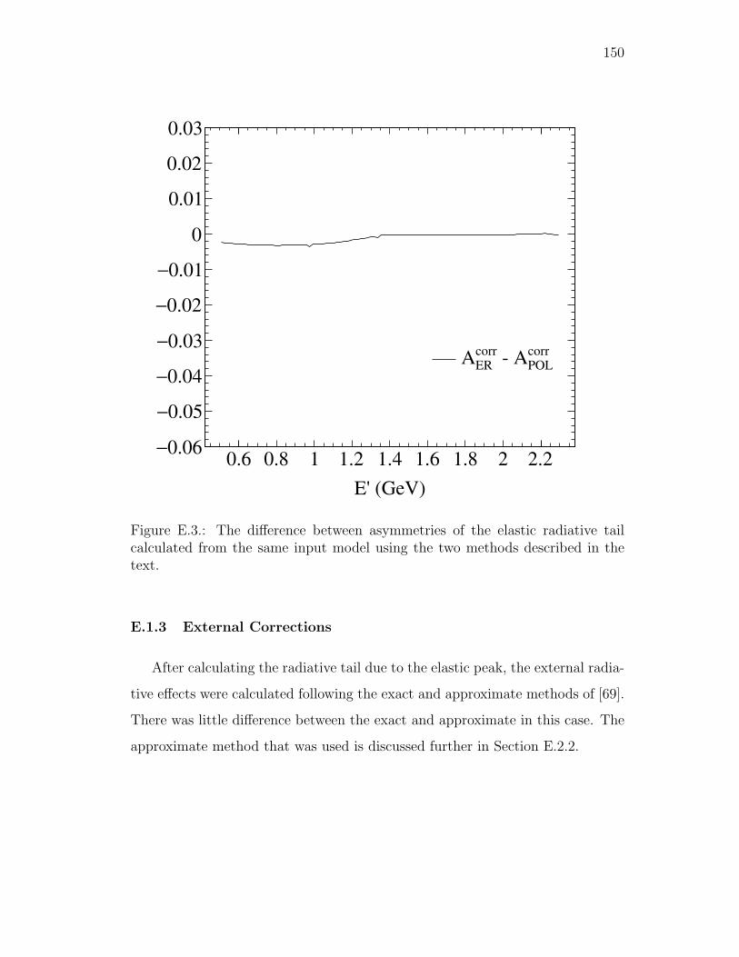
150

E' (GeV)

0.6 0.8 1 1.2 1.4 1.6 1.8 2 2.20.06−

0.05−

0.04−

0.03−

0.02−

0.01−

0

0.01

0.02

0.03

POLcorr - AER

corrA

Figure E.3.: The difference between asymmetries of the elastic radiative tailcalculated from the same input model using the two methods described in thetext.

E.1.3 External Corrections

After calculating the radiative tail due to the elastic peak, the external radia-

tive effects were calculated following the exact and approximate methods of [69].

There was little difference between the exact and approximate in this case. The

approximate method that was used is discussed further in Section E.2.2.

151

E.2 The Inelastic Radiative Tail

E.2.1 Internal Corrections

It was found that there are not any noticeable differences between the stan-

dard treatment [69] and the polarized treatment [111]. Furthermore, the equiva-

lent radiator method, which approximates the internal radiative effects by adding

some radiators (see equation 2.7 of [108]) to the target radiation length, works

quite well as shown by Figure E.4.

E' (GeV)

0.6 0.8 1 1.2 1.4 1.6 1.8 2 2.2

(n

b/G

eV/s

r)Ω

dE

'dσd

0

1

2

3

4

5

6

Internal Inelastic Radiative Tail

POLRAD2.0 Born

POLRAD2.0 IRT

RADCOR Born

RADCOR IRT (FORTRAN)

RADCOR IRT (C++)

InSANE Born

InSANE Polarized IRT

InSANE Equivalent radiator

° = 0targetθ

° = 40eθ

E = 5.89 GeV

Figure E.4.: Comparisons between different codes and methods for calculatingthe internal contribution to the inelastic radiative tail

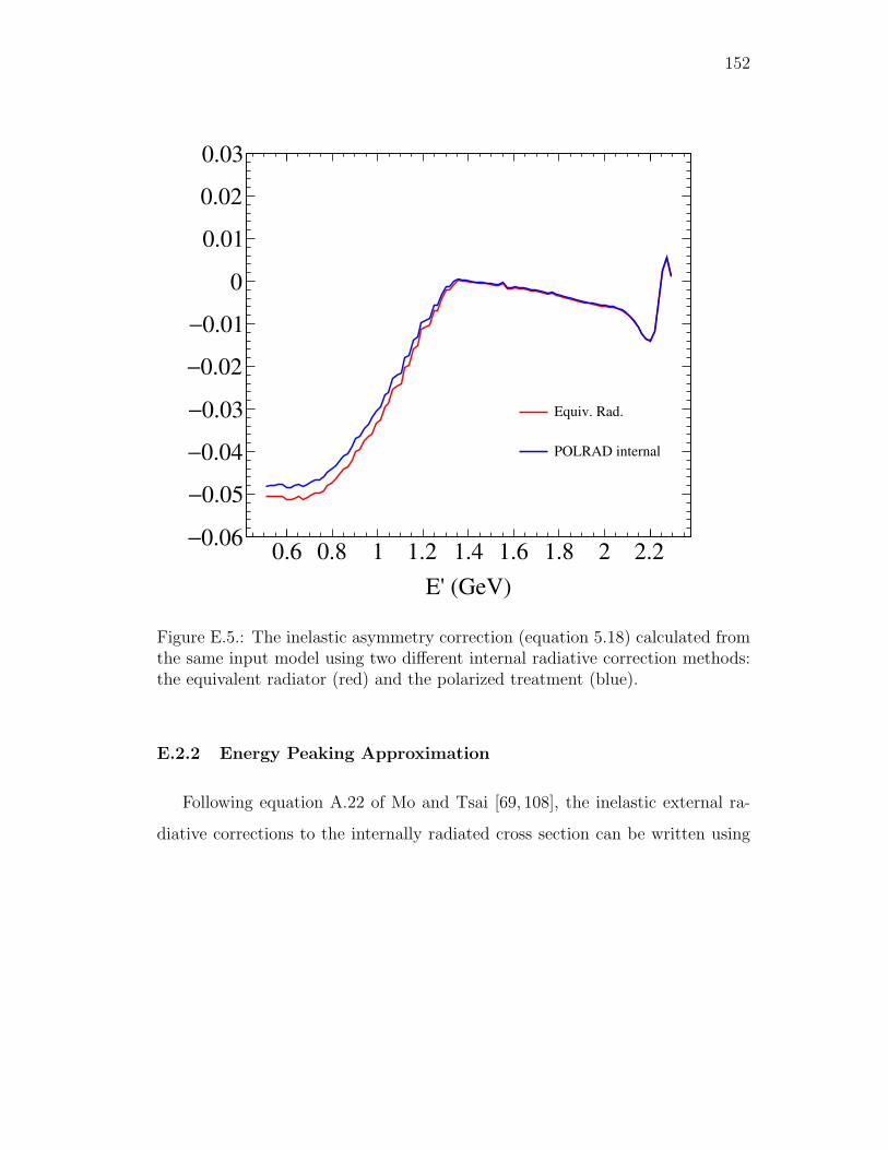
152

E' (GeV)

0.6 0.8 1 1.2 1.4 1.6 1.8 2 2.20.06−

0.05−

0.04−

0.03−

0.02−

0.01−

0

0.01

0.02

0.03

Equiv. Rad.

POLRAD internal

Figure E.5.: The inelastic asymmetry correction (equation 5.18) calculated fromthe same input model using two different internal radiative correction methods:the equivalent radiator (red) and the polarized treatment (blue).

E.2.2 Energy Peaking Approximation

Following equation A.22 of Mo and Tsai [69, 108], the inelastic external ra-

diative corrections to the internally radiated cross section can be written using

153

the energy peaking approximation. The energy peaking approximation for the

inelastic radiative can be modified to include beam depolarization effects

σt+r(Es, Ep, T ) = eδs+δpσr(Es, Ep, T )

+ eδs/2∫ Es−∆

Esmin(Ep)

[1−D(Es, E′s, Z)] Ie(Es, E

′s, T )σr(E

′s, Ep, T )dE

′s

+ eδp/2∫ Epmax(Es)

Ep+∆

Ie(E′p, Ep, T )σr(Es, E

′p, T )dE

′p .

(E.3)

where D is the beam depolarization factor calculated following [114]. In general

the size of the depolarization is very small.

W (GeV)

1 1.5 2 2.5 3 3.5

(n

b/G

eV/s

r)Ω

/dE

d1

80

σd

3−10

2−10

1−10

1

10

Figure E.6.: A comparison of the inelastic radiative tail for different cross models.

154

W (GeV)

1 1.5 2 2.5 3 3.50

0.1

0.2

0.3

0.4

0.5

0.6

0.7

0.8

0.9

1

Figure E.7.: The asymmetries of the inelastic cross sections shown in Figure E.6.

E.3 Comparing Codes

A comparison between the various codes and approximations are shown in

Figure E.4 where the input Born cross sections (dashed) are identical and used to

calculate the internal inelastic radiative tail. The existing Fortran codes RADCOR

[115–117] and POLRAD [113] are shown in addition to a C++ implementation of

RADCOR [117] and the newly developed radiative corrections code which is part

of the InSANE [65] C++ libraries. All the codes are in agreement except the

POLRAD.

155

W (GeV)

1 1.5 2 2.5 3 3.50.1−

0.08−

0.06−

0.04−

0.02−

0

0.02

0.04

0.06

0.08

0.1

E=5.9 GeVBorn -AIRTA E=5.9 GeVBorn -AIRTA

Figure E.8.: The inelastic asymmetry correction calculated using two very dif-ferent cross section models.

E.3.1 POLRAD

The InSANE inelastic tail shown was calculated following the same method

as POLRAD. After a lot of investigation, it was concluded that the discrepancy

shown in Figure E.4 is due to the integration subroutine used in POLRAD.

Upon close inspection it was found that there are a number of discrepancies

between what is written in the Fortran code and the POLRAD manual [113]. They

are reported here for future reference and documentation purposes.

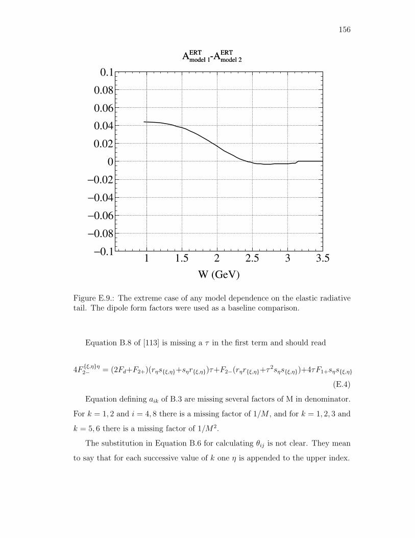
156

W (GeV)

1 1.5 2 2.5 3 3.50.1−

0.08−

0.06−

0.04−

0.02−

0

0.02

0.04

0.06

0.08

0.1

ERTmodel 2-AERT

model 1A ERTmodel 2-AERT

model 1A

Figure E.9.: The extreme case of any model dependence on the elastic radiativetail. The dipole form factors were used as a baseline comparison.

Equation B.8 of [113] is missing a τ in the first term and should read

4Fξ,ηη2− = (2Fd+F2+)(rηsξ,η+sηrξ,η)τ+F2−(rηrξ,η+τ

2sηsξ,η)+4τF1+sηsξ,η

(E.4)

Equation defining aik of B.3 are missing several factors of M in denominator.

For k = 1, 2 and i = 4, 8 there is a missing factor of 1/M , and for k = 1, 2, 3 and

k = 5, 6 there is a missing factor of 1/M2.

The substitution in Equation B.6 for calculating θij is not clear. They mean

to say that for each successive value of k one η is appended to the upper index.

157

For the θij terms corresponding to elastic scattering, the substitution should

be

θij (τ) → θAij (τA) (E.5)

where the index A is also applied to θij, not just τ . In the POLRAD manual, the

suggestion is to use τA, but with θij unchanged. It is clear in their corresponding

code that this is not the case and θij should be used.

158

159

APPENDIX F

PAIR SYMMETRIC BACKGROUND CORRECTIONS

The primary source of background comes from photons that convert into elec-

tron/positron pairs in extra material at the target or detector material. A sim-

ulation was developed in order to understand this background. The following

sections provide the details for calculating the background contaminations and

dilutions used in the asymmetry analysis.

F.1 BETA Background subtraction

The correction for an experiment using a large magnetic spectrometer is

Cbg =1−RApair/Araw

1−R, (F.1)

where R = npair,e+/ndis,e− and Apair is the positron asymmetry. Note that there

is also the measured ratio, r = npair,e+/ntotal,e− = R/(1 + R) which is often

(incorrectly) interchanged with R.

The equations above are correct for an experiment which only detects elec-

trons or high has a high positron rejection efficiency. However, for the case at

hand, BETA was in an open configuration and detected both charges. Therefore,

for each positron detected there is a corresponding electron, so a factor of two

must be added to each R in the equation above. Thus the total rate would be

ntotal = ndis + 2npair

= ndis(1 + 2R)

160

or

ndis = ntotal1

1 + 2R

npair = ntotal2R

1 + 2R

It should be noted that due to the up-down symmetry of the target magnet,

positron tracks are reconstructed the same as a positron track.

Using these definitions the correction can be split into a dilution correction

and a contamination correction due to Apair.

Acorr =

(

1

1− 2R

)

Araw −(

2RApair1− 2R

)

=

(

ndisndis − 2npair

)

Araw −(

2npairApairndis − 2npair

)

=

(

1

fbg

)

Araw −(

CAbg

)

F.2 Background Simulation

A simulation was developed to include all the target materials. The event gen-

erator sampled the inclusive electron cross section, inclusive photo- and electro-

production cross sections for neutral pions. The pion cross sections used were

obtained from Oscar Rondon’s fit [68] to the world data for kinematics relevant

to this experiment.

Results from the simulation are shown in Figure F.1. The impact of the

Cerenkov ADC window cut (discussed in section 5.4) can been seen in Figure F.2

which shows the electron positron ratio. This cut is especially important at high

energies where the relative size of the background is reduced by nearly a factor

of two.

161

Energy (GeV)

0.6 0.8 1 1.2 1.4 1.6 1.8 2

210

310

410 no window cut

window cut

e- no window

no windowπ

with window cutπ

Figure F.1.: The energy distribution of the reconstruction of simulated events.The blue curve shows the relative yield for events that originate with a scatteredelectron. The green and pink curves show the diluting background events withand without a Cerenkov ADC window cut. Similarly, the red and black showthe sum of all events with and with the window cut.

Energy (GeV)

0.6 0.8 1 1.2 1.4 1.6 1.8 20

0.2

0.4

0.6

0.8

1

1.2

No Window cut

Window cut

Figure F.2.: The ratio of positrons to electrons from simulation with and withouta Cerenkov ADC window cut applied.

162

163

APPENDIX G

ERROR ANALYSIS

G.1 Statistical Uncertainty

The statistical uncertainty on the raw asymmetry is

(σstatAraw

)2 =4n1n2

(n1 + n2)3(G.1)

where n1 and n2 are the raw counting rates for the two electron helicities. When

these are corrected for charge and live time (see equation 5.9) the statistical

uncertainty becomes

(σstatAexp

)2 =(A2

LT − 1)2(A2Q − 1)2(σstat

Araw)2

(AQAraw + ALT (Araw − AQ)− 1)4(G.2)

where the live-time asymmetry is

ALT =L1 − L2

L1 + L2

, (G.3)

the charge asymmetry is

AQ =Q1 −Q2

Q1 +Q2

, (G.4)

and where L1,2 and Q1,2 are the live-times and accumulated charge for each

helicity.

From equation 5.10 it follows that the statistical uncertainty after target

dilution, target polarization and beam polarization corrections becomes

(σstatAmeas

)2 =

(

σstatAexp

fPBPT

)2

(G.5)

164

Similarly, from equation 5.12 the statistical uncertainty after background correc-

tions is

(σstatABG

corr)2 =

(

σstatAmeas

(1− 2R)

)2

. (G.6)

Finally, the statical uncertainty after subtracting the elastic radiative tail is

(σstatAel

corr)2 =

(

σstatABG

corr(Σel + Σin)

Σin

)2

. (G.7)

It is worth noting that the inelastic correction is purely a systematic uncertainty

and does not affect the size of the statistical error bars.

G.2 Systematic Uncertainties

A summary of the estimated systematic uncertainties are given in table G.1.

In the following text the estimated systematic uncertainty of an input quantity,

e.g. X, is indicated by δX .

G.2.1 Measured Asymmetry

Using the raw asymmetry calculated in equation 5.7, the charge and live time

corrected asymmetry in equation 5.8 can be rewritten as

Am =ALT + AQ − Araw − ALTAQArawAQAraw + ALT (Araw − AQ)− 1

. (G.8)

From equation G.8 it is clear that the measured asymmetry only depends

on the charge and live-time asymmetries, and not their absolute values. The

systematic uncertainty after correcting for the charge and live-time asymmetries

is

(σAm)2 =

(A2raw − 1)

2[

(A2LT − 1)

2δ2AQ

+(

A2Q − 1

)2δ2ALT

]

(1− Araw(ALT + AQ) + ALTAQ)4(G.9)

165

where δAQis the charge asymmetry systematic uncertainty and δALT

is the live-

time systematic uncertainty.

G.2.2 Physics Asymmetry

The asymmetry corrected for target dilution, target polarization, and beam

polarization, equation 5.10, gives the total systematic uncertainty

(σAmeas)2 =

(σAexp)2

f 2P 2BP

2T

+A2

exp

(

f 2P 2Tδ

2PB

+ P 2BP

2Tδ

2f + f 2P 2

Bδ2PT

)

f 4P 4BP

4T

(G.10)

where

G.2.3 Pair Symmetric Background Corrected Asymmetry

From the equation 5.12 the systematic uncertainty with the pair symmetric

background correction becomes

(σABGcorr

)2 =σ2Ameas

(1− 2R)2+

4(1− 2R)2R2δ2Apair+ 4(Ameas − Apair)

2δ2R

(1− 2R)4(G.11)

where δR is the uncertainty on the estimated ratio of electrons to positrons and

δApairis the pair background asymmetry (see Appendix F for more details).

G.2.4 Elastic Radiative Tail Correction

The total inelastic asymmetry is calculated by subtracted the elastic radiative

tail contribution. From equation 5.15 the systematic uncertainty is

(σAelcorr

)2 =(σABG

corr)2(Σel + Σin)

2

Σ2in

+δ2Σin

(∆el − ABGcorrΣel)2 +

(

δ2∆el+ (ABGcorr)

2δ2Σel

)

Σ2in

Σ4in

(G.12)

where δ∆in,elis the systematic uncertainty in the inelastic and elastic cross section

differences and δΣin,elis the total uncertainty of their sum.

166

G.2.5 Inelastic Radiative Tail Correction

Equation G.12 shows that the complete treatment of elastic tail requires an

unfolding of procedure since quantities like ∆in are the primary focus of such a

measurement. The inelastic radiative tail correction, equation 5.18, introduces

a single systematic uncertainty δin. The main source of this uncertainty should

come from the treatment of the radiative, assuming a full measurement was com-

pleted, as outlined by Mo and Tsai [69], in order to proceed to unfold the Born

cross sections. However, since only asymmetries were measured this uncertainty

also reflects an uncertainty from a model or fit dependence of the cross sections.

G.3 Systematic Uncertainty Estimates

Table G.1.: Systematic uncertainty estimates.

symbol δ A180 Relative Unc.Charge asymmetry AQ 0.0015 3.0%Live-time asymmetry AL 0.003 6.0%Beam polarization Pb 0.015 1%Target polarization Pt 0.04 6%Dilution factor f 0.02 9%Positron to electron ratio R 0.02Pair Symmetric Background Asymmetry Apair 0.04Inelastic cross section sum Σin 0.01Elastic cross section sum Σel 0.005Elastic cross section difference ∆el 0.005

167

APPENDIX H

TABLES OF RESULTS

This appendix contains tables of results. More useful and detailed data files of

the tables below will be made available upon request1.

H.1 A1 and A2 with 4.7 GeV Beam

The tables H.1–H.3 show the results for Ap1 and tables H.4–H.6 show the

results for Ap2 using a 4.7 GeV electron beam. The data is split into large Q2

bins and binned in x. The mean values of Q2, W , θ, and φ for each bin are also

shown in each table.

Table H.1.: A1 results for 1.0 < Q2 < 2.25 and E = 4.7 GeV.

x Q2 [GeV2] W [GeV] E ′ [GeV] θ [deg.] φ [deg.] A δA (stat.) δA (syst.)0.20352 1.4625 2.5698 0.90652 34.007 16.341 0.25963 0.095347 0.0972870.21136 1.512 2.5538 0.92377 34.278 16.238 0.48746 0.088355 0.0983270.21982 1.5671 2.538 0.93703 34.69 15.688 0.36567 0.080835 0.101560.22908 1.6287 2.5221 0.94707 35.227 14.829 0.5547 0.07231 0.108710.23908 1.6972 2.5062 0.95291 35.912 13.663 0.39612 0.063408 0.110420.25 1.7731 2.4897 0.95657 36.702 13.405 0.51532 0.054099 0.109250.26191 1.8518 2.4694 0.96827 37.329 13.308 0.42719 0.047256 0.11370.27503 1.9366 2.4462 0.98371 37.923 13.44 0.37375 0.041773 0.111390.28953 2.0292 2.4204 1.0012 38.525 13.495 0.47109 0.03745 0.117390.30522 2.1202 2.3886 1.0341 38.745 13.749 0.49551 0.035509 0.1240.32176 2.1598 2.3309 1.1582 36.796 13.558 0.4633 0.04665 0.0692950.34205 2.1664 2.2468 1.3602 33.785 16.252 0.56538 0.083776 0.0679550.36306 2.2077 2.1804 1.4949 32.446 16.945 0.76938 0.14499 0.0747450.38822 2.2041 2.0868 1.7035 30.345 15.656 1.0569 1.7586 0.38687

1whit@jlab.org or whit@temple.edu

168

Table H.2.: A1 results for 2.25 < Q2 < 3.5 and E = 4.7 GeV.

x Q2 [GeV2] W [GeV] E ′ [GeV] θ [deg.] φ [deg.] A δA (stat.) δA (syst.)0.30943 2.2642 2.4359 0.83684 44.421 12.698 -0.058687 0.25086 0.110540.31826 2.2879 2.4045 0.90497 42.911 14.671 0.3176 0.079285 0.0792630.3292 2.32 2.3681 0.98041 41.504 14.709 0.32426 0.054153 0.0772490.34081 2.3677 2.3365 1.0339 40.849 14.044 0.62097 0.048006 0.0762920.35304 2.4249 2.3073 1.0758 40.562 14.136 0.42527 0.047126 0.071720.36562 2.4829 2.2776 1.1172 40.315 14.393 0.59717 0.047155 0.0737880.37846 2.538 2.2466 1.1624 40.011 14.569 0.51116 0.048075 0.071480.39154 2.6008 2.2182 1.1963 39.933 14.629 0.62702 0.049936 0.074850.40486 2.6669 2.1906 1.2259 39.938 14.56 0.58824 0.052723 0.0722970.41857 2.7346 2.1627 1.2546 39.972 14.55 0.59085 0.054976 0.0739290.43315 2.8047 2.1329 1.2855 39.984 14.535 0.64742 0.057031 0.0762010.44876 2.8781 2.101 1.3184 39.985 14.528 0.7132 0.059732 0.0844520.46561 2.9554 2.0666 1.3536 39.986 14.594 0.55167 0.063287 0.0774990.48382 3.0383 2.0299 1.3895 40.006 14.716 0.68841 0.067317 0.090240.50349 3.1244 1.99 1.4292 39.991 14.75 0.69553 0.072711 0.0916880.52484 3.2101 1.9456 1.4766 39.85 14.847 0.69668 0.079665 0.0608260.54763 3.2803 1.8945 1.5439 39.348 14.749 0.77289 0.095393 0.0661470.57273 3.3089 1.8298 1.6571 38.053 13.943 0.9081 0.13149 0.066040.60006 3.3117 1.7571 1.7946 36.502 12.109 0.23618 0.1901 0.0634080.63127 3.2874 1.6735 1.9606 34.688 14.008 0.25816 0.28117 0.0741290.66538 3.3162 1.5964 2.0798 33.76 15.856 0.26182 0.50049 0.114840.7037 3.3703 1.5164 2.1837 33.178 15.974 0.43637 0.63244 0.0662170.7418 3.443 1.4419 2.2624 32.935 15.869 2.3016 1.3922 0.17780.78193 3.4267 1.3552 2.3977 31.906 14.748 -6.8596 6.7275 0.50808

Table H.3.: A1 results for 3.5 < Q2 < 5.0 and E = 4.7 GeV.

x Q2 [GeV2] W [GeV] E ′ [GeV] θ [deg.] φ [deg.] A δA (stat.) δA (syst.)0.50023 3.506 2.0936 0.99421 51.161 14.292 -6.0859e-05 11335 0.0146880.513 3.5328 2.0577 1.0645 49.514 16.622 0.49558 1.0189 0.252660.5303 3.5577 2.0079 1.1597 47.515 15.98 0.62748 0.52556 0.171220.54997 3.5548 1.9466 1.2909 44.884 16.701 0.4341 0.25899 0.0750740.56805 3.5781 1.8977 1.3791 43.487 16.9 0.64018 0.17308 0.0785730.58767 3.6214 1.8496 1.4521 42.607 17.432 0.72314 0.15909 0.0730780.60773 3.6631 1.8013 1.5239 41.814 16.758 0.83724 0.158 0.0655180.62826 3.7162 1.7547 1.584 41.299 15.997 0.58923 0.16022 0.0613620.64943 3.7889 1.7103 1.6271 41.149 15.491 0.71531 0.15536 0.0536390.6719 3.8595 1.6627 1.675 40.938 15.659 0.52603 0.17646 0.0545550.69607 3.9367 1.6121 1.7222 40.777 15.39 0.2962 0.22298 0.0679890.72194 4.0196 1.5582 1.769 40.655 15.879 1.0881 0.25652 0.078980.75012 4.0921 1.4977 1.8289 40.365 15.314 0.17798 0.24574 0.055380.78049 4.1533 1.431 1.9003 39.919 15.775 1.2868 0.34803 0.102140.81381 4.2607 1.3618 1.9462 39.95 15.82 1.3032 0.44564 0.11780.84916 4.3644 1.2864 1.9973 39.908 16.237 -0.51154 0.59372 0.140280.88881 4.4592 1.199 2.0626 39.695 15.924 1.8362 0.76968 0.1587

169

Table H.4.: A2 results for 1.0 < Q2 < 2.25 and E = 4.7 GeV.

x Q2 [GeV2] W [GeV] E ′ [GeV] θ [deg.] φ [deg.] A δA (stat.) δA (syst.)0.20352 1.4625 2.5698 0.90652 34.007 16.341 0.30393 0.30418 0.0972870.21136 1.512 2.5538 0.92377 34.278 16.238 0.13267 0.27045 0.0983270.21982 1.5671 2.538 0.93703 34.69 15.688 0.26911 0.23557 0.101560.22908 1.6287 2.5221 0.94707 35.227 14.829 -0.1416 0.20793 0.108710.23908 1.6972 2.5062 0.95291 35.912 13.663 -0.24028 0.17984 0.110420.25 1.7731 2.4897 0.95657 36.702 13.405 0.22828 0.15961 0.109250.26191 1.8518 2.4694 0.96827 37.329 13.308 0.12517 0.14412 0.11370.27503 1.9366 2.4462 0.98371 37.923 13.44 0.22453 0.13122 0.111390.28953 2.0292 2.4204 1.0012 38.525 13.495 -0.0097248 0.11924 0.117390.30522 2.1202 2.3886 1.0341 38.745 13.749 0.1199 0.1121 0.1240.32176 2.1598 2.3309 1.1582 36.796 13.558 0.20589 0.13765 0.0692950.34205 2.1664 2.2468 1.3602 33.785 16.252 -0.033791 0.23739 0.0679550.36306 2.2077 2.1804 1.4949 32.446 16.945 0.068401 0.36228 0.0747450.38822 2.2041 2.0868 1.7035 30.345 15.656 -0.19658 0.62789 0.38687

Table H.5.: A2 results for 2.25 < Q2 < 3.5 and E = 4.7 GeV.

x Q2 [GeV2] W [GeV] E ′ [GeV] θ [deg.] φ [deg.] A δA (stat.) δA (syst.)0.30943 2.2642 2.4359 0.83684 44.421 12.698 0.17507 0.83278 0.110540.31826 2.2879 2.4045 0.90497 42.911 14.671 -0.25417 0.279 0.0792630.3292 2.32 2.3681 0.98041 41.504 14.709 0.59718 0.18504 0.0772490.34081 2.3677 2.3365 1.0339 40.849 14.044 -0.16888 0.1551 0.0762920.35304 2.4249 2.3073 1.0758 40.562 14.136 0.061307 0.1501 0.071720.36562 2.4829 2.2776 1.1172 40.315 14.393 -0.084201 0.14805 0.0737880.37846 2.538 2.2466 1.1624 40.011 14.569 -0.17091 0.14989 0.071480.39154 2.6008 2.2182 1.1963 39.933 14.629 -0.045377 0.15224 0.074850.40486 2.6669 2.1906 1.2259 39.938 14.56 -0.16356 0.15717 0.0722970.41857 2.7346 2.1627 1.2546 39.972 14.55 0.15849 0.16247 0.0739290.43315 2.8047 2.1329 1.2855 39.984 14.535 -0.2418 0.16522 0.0762010.44876 2.8781 2.101 1.3184 39.985 14.528 -0.12462 0.17121 0.0844520.46561 2.9554 2.0666 1.3536 39.986 14.594 -0.16274 0.17877 0.0774990.48382 3.0383 2.0299 1.3895 40.006 14.716 0.16031 0.18641 0.090240.50349 3.1244 1.99 1.4292 39.991 14.75 -0.12856 0.20145 0.0916880.52484 3.2101 1.9456 1.4766 39.85 14.847 -0.0027396 0.2151 0.0608260.54763 3.2803 1.8945 1.5439 39.348 14.749 -0.087906 0.26114 0.0661470.57273 3.3089 1.8298 1.6571 38.053 13.943 -0.79499 0.3407 0.066040.60006 3.3117 1.7571 1.7946 36.502 12.109 0.93833 0.4501 0.0634080.63127 3.2874 1.6735 1.9606 34.688 14.008 1.4907 0.63519 0.0741290.66538 3.3162 1.5964 2.0798 33.76 15.856 0.58215 1.0772 0.114840.7037 3.3703 1.5164 2.1837 33.178 15.974 0.43353 1.3557 0.0662170.7418 3.443 1.4419 2.2624 32.935 15.869 -2.4572 3.1197 0.17780.78193 3.4267 1.3552 2.3977 31.906 14.748 2.1793 4.6673 0.50808

H.2 A1 and A2 with 5.9 GeV Beam

The tables H.1–H.3 show the results for Ap1 and tables H.4–H.6 show the

results for Ap2 using a 4.7 GeV electron beam. The data is split into large Q2

170

Table H.6.: A2 results for 3.5 < Q2 < 5.0 and E = 4.7 GeV.

x Q2 [GeV2] W [GeV] E ′ [GeV] θ [deg.] φ [deg.] A δA (stat.) δA (syst.)0.50023 3.506 2.0936 0.99421 51.161 14.292 0.00046781 16464 0.0146880.513 3.5328 2.0577 1.0645 49.514 16.622 2.4614 1.668 0.252660.5303 3.5577 2.0079 1.1597 47.515 15.98 -0.24733 0.98042 0.171220.54997 3.5548 1.9466 1.2909 44.884 16.701 -0.24966 0.55184 0.0750740.56805 3.5781 1.8977 1.3791 43.487 16.9 0.9192 0.42815 0.0785730.58767 3.6214 1.8496 1.4521 42.607 17.432 -0.55624 0.42848 0.0730780.60773 3.6631 1.8013 1.5239 41.814 16.758 0.083842 0.41521 0.0655180.62826 3.7162 1.7547 1.584 41.299 15.997 0.57516 0.41731 0.0613620.64943 3.7889 1.7103 1.6271 41.149 15.491 -0.09536 0.3964 0.0536390.6719 3.8595 1.6627 1.675 40.938 15.659 -0.24192 0.42985 0.0545550.69607 3.9367 1.6121 1.7222 40.777 15.39 0.57247 0.52459 0.0679890.72194 4.0196 1.5582 1.769 40.655 15.879 -1.1092 0.60961 0.078980.75012 4.0921 1.4977 1.8289 40.365 15.314 1.0997 0.55638 0.055380.78049 4.1533 1.431 1.9003 39.919 15.775 1.1022 0.76834 0.102140.81381 4.2607 1.3618 1.9462 39.95 15.82 -1.7362 0.982 0.11780.84916 4.3644 1.2864 1.9973 39.908 16.237 2.8097 1.2815 0.140280.88881 4.4592 1.199 2.0626 39.695 15.924 -1.6765 1.666 0.1587

Table H.7.: A1 results for 1.0 < Q2 < 2.25 and E = 5.9 GeV.

x Q2 [GeV2] W [GeV] E ′ [GeV] θ [deg.] φ [deg.] A δA (stat.) δA (syst.)0.20362 1.8843 2.8722 0.96029 33.757 17.852 0.16763 0.44475 0.201040.21143 1.9573 2.86 0.95869 34.501 15.919 0.24512 0.23354 0.13420.21992 2.0358 2.8461 0.95901 35.236 14.468 0.61591 0.15998 0.119040.2291 2.1219 2.8318 0.95649 36.07 13.455 0.36114 0.11698 0.103260.23787 2.1772 2.8028 1.0138 35.485 14.041 0.40027 0.13997 0.095259

bins and binned in x. The mean values of Q2, W , θ, and φ for each bin are also

shown in each table.

171

Table H.8.: A1 results for 2.25 < Q2 < 3.5 and E = 5.9 GeV.

x Q2 [GeV2] W [GeV] E ′ [GeV] θ [deg.] φ [deg.] A δA (stat.) δA (syst.)0.23624 2.254 2.8579 0.80873 40.224 14.194 -0.56309 0.64314 0.232270.24123 2.2801 2.8377 0.85582 39.326 11.56 0.070684 0.11511 0.0912540.24843 2.3299 2.8158 0.89493 38.903 12.032 0.27843 0.084565 0.0835410.25679 2.3913 2.793 0.9302 38.735 13.009 0.28901 0.074665 0.0779790.26567 2.4593 2.7708 0.95958 38.769 13.488 0.3061 0.067037 0.0840390.27506 2.536 2.7501 0.97938 39.044 13.741 0.29318 0.060881 0.0739310.28492 2.6199 2.7303 0.9926 39.448 13.671 0.38213 0.0563 0.0716630.29523 2.705 2.7086 1.0101 39.742 13.821 0.34028 0.053992 0.071990.30598 2.7909 2.685 1.0321 39.933 14.045 0.30994 0.052622 0.0714730.31717 2.8786 2.6602 1.0561 40.097 14.133 0.30211 0.052404 0.0655350.32874 2.969 2.6347 1.0799 40.282 14.105 0.33319 0.05263 0.0678830.34068 3.0611 2.6083 1.1045 40.46 14.042 0.43309 0.053388 0.0636030.35295 3.1546 2.5811 1.1297 40.624 13.867 0.4995 0.054303 0.0680220.36552 3.2475 2.5526 1.1582 40.709 13.744 0.4464 0.056089 0.0719410.37826 3.3273 2.5195 1.2053 40.32 13.349 0.3923 0.058641 0.0599090.39102 3.3757 2.4773 1.292 39.108 12.837 0.42781 0.070283 0.0676740.40392 3.3997 2.4283 1.4071 37.524 11.341 0.58736 0.10672 0.0651390.41722 3.3783 2.3661 1.5768 35.291 11.32 1.0351 0.25255 0.108150.4649 3.3713 2.1819 2.0271 30.841 13.972 0.14783 13080 0.000289150.48321 3.4156 2.1292 2.1246 30.294 13.805 0.21325 13319 0.00768010.50129 3.4476 2.0762 2.2263 29.715 13.83 0.4265 13605 0.00446830.52142 3.4695 2.0162 2.3453 29.023 14.35 -0.43975 14002 0.0042626

Table H.9.: A1 results for 3.5 < Q2 < 5.0 and E = 5.9 GeV.

x Q2 [GeV2] W [GeV] E ′ [GeV] θ [deg.] φ [deg.] A δA (stat.) δA (syst.)0.37499 3.5357 2.6026 0.86703 49.218 15.718 -0.14677 10805 0.0902940.38682 3.5544 2.5524 0.99534 45.944 15.861 0.3607 0.21522 0.115680.39881 3.5865 2.5073 1.1002 43.801 14.642 0.42521 0.094219 0.0706820.41227 3.6347 2.462 1.1946 42.298 13.951 0.39227 0.070549 0.0617250.42655 3.7075 2.4215 1.261 41.586 12.997 0.47112 0.066714 0.0611840.44179 3.803 2.3843 1.3054 41.402 12.831 0.48354 0.069772 0.0622870.45784 3.9052 2.346 1.3474 41.302 12.694 0.47384 0.074153 0.0600890.47452 4.0105 2.3066 1.3889 41.23 12.64 0.43891 0.078877 0.0594290.49188 4.1186 2.2658 1.4307 41.179 12.453 0.62243 0.08467 0.0777940.50985 4.2274 2.2233 1.4742 41.111 12.359 0.42467 0.092491 0.0637480.52835 4.339 2.18 1.5164 41.073 12.38 0.62727 0.10016 0.0789070.54741 4.4498 2.1349 1.5609 40.994 12.277 0.73748 0.10952 0.0718250.5669 4.5649 2.0896 1.6017 40.968 12.307 0.69256 0.12331 0.066210.58697 4.675 2.0418 1.6485 40.825 12.388 0.5756 0.13563 0.075460.60678 4.7503 1.9894 1.7209 40.226 12.255 0.43545 0.15864 0.0751890.6274 4.7767 1.9278 1.8357 38.969 11.981 0.68319 0.21258 0.102190.64849 4.8049 1.8666 1.9442 37.929 10.747 0.75308 0.31793 0.128720.6703 4.796 1.7997 2.0792 36.612 9.2617 1.1616 0.55475 0.202090.6944 4.7212 1.7198 2.2682 34.722 10.72 2.6476 1.5714 0.22924

172

Table H.10.: A1 results for 5.0 < Q2 < 7.5 and E = 5.9 GeV.

x Q2 [GeV2] W [GeV] E ′ [GeV] θ [deg.] φ [deg.] A δA (stat.) δA (syst.)0.56608 5.0198 2.1744 1.1664 50.6 12.938 -0.00052565 10938 0.00242090.60158 5.089 2.0618 1.3835 46.625 12.665 -0.33716 1.4996 0.324680.62172 5.0986 1.9956 1.5221 44.357 12.701 0.23012 0.31916 0.128910.64306 5.1658 1.9359 1.6119 43.347 13.165 0.18436 0.23454 0.0920910.66629 5.2445 1.8727 1.6981 42.548 13.505 0.50021 0.2244 0.0870020.69036 5.3297 1.8084 1.7788 41.907 12.842 0.68897 0.23825 0.0673590.71554 5.457 1.7462 1.8288 41.83 12.587 0.55959 0.24932 0.0941480.74161 5.5839 1.6809 1.8805 41.715 12.749 1.0391 0.27329 0.081030.76849 5.7186 1.6132 1.9274 41.702 12.654 0.50873 0.38323 0.124180.79597 5.8518 1.5427 1.9751 41.682 12.818 0.042863 0.43279 0.116270.82404 5.9894 1.4693 2.0195 41.694 13.014 1.3087 0.48957 0.135210.85304 6.1288 1.3913 2.0643 41.715 13.42 -1.1049 0.67396 0.206490.88238 6.2682 1.3097 2.1074 41.765 13.229 0.14824 0.95516 0.303960.91264 6.3893 1.2213 2.1619 41.646 12.7 0.76978 1.4268 0.35395

Table H.11.: A2 results for 1.0 < Q2 < 2.25 and E = 5.9 GeV.

x Q2 [GeV2] W [GeV] E ′ [GeV] θ [deg.] φ [deg.] A δA (stat.) δA (syst.)0.20362 1.8843 2.8722 0.96029 33.757 17.852 0.1092 0.12675 0.201040.21143 1.9573 2.86 0.95869 34.501 15.919 0.2971 0.10398 0.13420.21992 2.0358 2.8461 0.95901 35.236 14.468 -0.075179 0.090333 0.119040.2291 2.1219 2.8318 0.95649 36.07 13.455 0.091437 0.079289 0.103260.23787 2.1772 2.8028 1.0138 35.485 14.041 0.097685 0.082258 0.095259

Table H.12.: A2 results for 2.25 < Q2 < 3.5 and E = 5.9 GeV.

x Q2 [GeV2] W [GeV] E ′ [GeV] θ [deg.] φ [deg.] A δA (stat.) δA (syst.)0.23624 2.254 2.8579 0.80873 40.224 14.194 -3.4667 0.93863 0.232270.24123 2.2801 2.8377 0.85582 39.326 11.56 0.156 0.13588 0.0912540.24843 2.3299 2.8158 0.89493 38.903 12.032 0.01234 0.093773 0.0835410.25679 2.3913 2.793 0.9302 38.735 13.009 0.05787 0.078812 0.0779790.26567 2.4593 2.7708 0.95958 38.769 13.488 0.10671 0.069514 0.0840390.27506 2.536 2.7501 0.97938 39.044 13.741 0.0071657 0.063885 0.0739310.28492 2.6199 2.7303 0.9926 39.448 13.671 0.03653 0.060738 0.0716630.29523 2.705 2.7086 1.0101 39.742 13.821 0.11883 0.059 0.071990.30598 2.7909 2.685 1.0321 39.933 14.045 -0.0017938 0.058143 0.0714730.31717 2.8786 2.6602 1.0561 40.097 14.133 0.032635 0.057696 0.0655350.32874 2.969 2.6347 1.0799 40.282 14.105 -0.0064269 0.057945 0.0678830.34068 3.0611 2.6083 1.1045 40.46 14.042 -0.090434 0.058523 0.0636030.35295 3.1546 2.5811 1.1297 40.624 13.867 -0.062238 0.059637 0.0680220.36552 3.2475 2.5526 1.1582 40.709 13.744 0.067182 0.061356 0.0719410.37826 3.3273 2.5195 1.2053 40.32 13.349 0.062337 0.065437 0.0599090.39102 3.3757 2.4773 1.292 39.108 12.837 0.13199 0.077686 0.0676740.40392 3.3997 2.4283 1.4071 37.524 11.341 0.12085 0.10286 0.0651390.41722 3.3783 2.3661 1.5768 35.291 11.32 0.065893 0.15736 0.108150.4649 3.3713 2.1819 2.0271 30.841 13.972 -0.70349 1013.5 0.000289150.48321 3.4156 2.1292 2.1246 30.294 13.805 -0.94976 1224.2 0.00768010.50129 3.4476 2.0762 2.2263 29.715 13.83 -1.7781 1451.3 0.00446830.52142 3.4695 2.0162 2.3453 29.023 14.35 1.703 1728 0.0042626

173

Table H.13.: A2 results for 3.5 < Q2 < 5.0 and E = 5.9 GeV.

x Q2 [GeV2] W [GeV] E ′ [GeV] θ [deg.] φ [deg.] A δA (stat.) δA (syst.)0.37499 3.5357 2.6026 0.86703 49.218 15.718 0.95135 1044.7 0.0902940.38682 3.5544 2.5524 0.99534 45.944 15.861 -0.21184 0.1723 0.115680.39881 3.5865 2.5073 1.1002 43.801 14.642 -0.043533 0.1064 0.0706820.41227 3.6347 2.462 1.1946 42.298 13.951 0.10673 0.083765 0.0617250.42655 3.7075 2.4215 1.261 41.586 12.997 -0.045687 0.077164 0.0611840.44179 3.803 2.3843 1.3054 41.402 12.831 0.043436 0.077634 0.0622870.45784 3.9052 2.346 1.3474 41.302 12.694 0.090392 0.080702 0.0600890.47452 4.0105 2.3066 1.3889 41.23 12.64 0.08416 0.084907 0.0594290.49188 4.1186 2.2658 1.4307 41.179 12.453 0.12974 0.089936 0.0777940.50985 4.2274 2.2233 1.4742 41.111 12.359 0.1306 0.096092 0.0637480.52835 4.339 2.18 1.5164 41.073 12.38 0.054358 0.10365 0.0789070.54741 4.4498 2.1349 1.5609 40.994 12.277 0.014378 0.11388 0.0718250.5669 4.5649 2.0896 1.6017 40.968 12.307 0.053614 0.12654 0.066210.58697 4.675 2.0418 1.6485 40.825 12.388 -0.0094425 0.14187 0.075460.60678 4.7503 1.9894 1.7209 40.226 12.255 -0.029734 0.17404 0.0751890.6274 4.7767 1.9278 1.8357 38.969 11.981 -0.15858 0.23599 0.102190.64849 4.8049 1.8666 1.9442 37.929 10.747 -0.49136 0.30364 0.128720.6703 4.796 1.7997 2.0792 36.612 9.2617 0.5095 0.4334 0.202090.6944 4.7212 1.7198 2.2682 34.722 10.72 0.034691 0.67964 0.22924

Table H.14.: A2 results for 5.0 < Q2 < 7.5 and E = 5.9 GeV.

x Q2 [GeV2] W [GeV] E ′ [GeV] θ [deg.] φ [deg.] A δA (stat.) δA (syst.)0.56608 5.0198 2.1744 1.1664 50.6 12.938 0.0044827 99.403 0.00242090.60158 5.089 2.0618 1.3835 46.625 12.665 0.38026 0.42838 0.324680.62172 5.0986 1.9956 1.5221 44.357 12.701 -0.46761 0.27008 0.128910.64306 5.1658 1.9359 1.6119 43.347 13.165 0.032125 0.242 0.0920910.66629 5.2445 1.8727 1.6981 42.548 13.505 0.28666 0.2359 0.0870020.69036 5.3297 1.8084 1.7788 41.907 12.842 -0.21936 0.25199 0.0673590.71554 5.457 1.7462 1.8288 41.83 12.587 0.26626 0.26951 0.0941480.74161 5.5839 1.6809 1.8805 41.715 12.749 -0.74906 0.28759 0.081030.76849 5.7186 1.6132 1.9274 41.702 12.654 0.20719 0.37653 0.124180.79597 5.8518 1.5427 1.9751 41.682 12.818 -0.26055 0.42538 0.116270.82404 5.9894 1.4693 2.0195 41.694 13.014 -0.52174 0.50673 0.135210.85304 6.1288 1.3913 2.0643 41.715 13.42 -0.10637 0.74638 0.206490.88238 6.2682 1.3097 2.1074 41.765 13.229 0.38041 1.0629 0.303960.91264 6.3893 1.2213 2.1619 41.646 12.7 -0.50039 1.6488 0.35395