measurement of specialization – the choice of · pdf filemeasurement of specialization...
TRANSCRIPT

FIW, a collaboration of WIFO (www.wifo.ac.at), wiiw (www.wiiw.ac.at) and WSR (www.wsr.ac.at)
FIW – Working Paper
Measurement of Specialization – The Choice of Indices
Nicole Palan
This paper compares nine common specialization indices, discussing their properties, strengths and weaknesses. In order to unravel the differences between the indices they are applied to European employment structures in 2005, spanning 51 industries and 24 European countries. The resulting heterogeneity levels differ largely between relative and absolute specialization measures, but also within these two groups of indices. As results are highly dependent on which measure is employed, it is important to be aware of carefully choosing appropriate indices in empirical studies in order to attain appropriate conclusions and conduct sound economic policy. JEL : B41, C82, O47 Keywords: specialization indices, industry structure, comparison of indices
Nicole Palan, Graz Schumpeter Centre, Universitätsstraße 15/FE, 8010 Graz, Austria. Tel: +43-(0)316-380 3596, e-mail: [email protected]. The author likes to thank Claudia Schmiedeberg, Heinz D. Kurz, Henryk Gurgul, Stefan Palan, David Colander and Mike Dietrich for their comments and help on the paper.
Abstract
The author
FIW Working Paper N° 62 December 2010


Measurement of Specialization - The Choice of Indices
Nicole Palan*
Abstract:
This paper compares nine common specialization indices, discussing their properties,
strengths and weaknesses. In order to unravel the differences between the indices
they are applied to European employment structures in 2005, spanning 51 industries
and 24 European countries. The resulting heterogeneity levels differ largely between
relative and absolute specialization measures, but also within these two groups of
indices. As results are highly dependent on which measure is employed, it is
important to be aware of carefully choosing appropriate indices in empirical studies
in order to attain appropriate conclusions and conduct sound economic policy.
Keywords: specialization indices, industry structure, comparison of indices
JEL-No.: B41, C82, O47
Nicole Palan, Graz Schumpeter Centre, Universitätsstraße 15/FE, 8010 Graz, Austria. Tel: +43-(0)316-380
3596, e-mail: [email protected].
The author likes to thank Claudia Schmiedeberg, Heinz D. Kurz, Henryk Gurgul, Stefan Palan, David
Colander and Mike Dietrich for their comments and help on the paper.

Introduction
Due to the increasing interest on the effects of economic integration on the
specialization of countries, the necessity to measure heterogeneity across countries
as well as its effects on the competitiveness of individual countries has risen. Empirical
research on international trade and international specialization patterns uses a wide
array of statistical tools, ranging from simple descriptive indicators to complex
econometric techniques. Yet there seems to have been no agreement on which
index is best to capture specialization, although the empirical results depend heavily
on the statistical methods and measures employed.
In this paper we thus aim to compare nine common specialization indices, discussing
their properties, strengths and weaknesses. In order to unravel the differences
between the indices, we apply them to European employment structures in 2005,
spanning 51 industries and 24 European Countries. Note that we restrict our analysis
to the calculation of specialization indices, leaving out such issues as the
development of geographic concentration patterns, the difference between
heterogeneity arising from unrelated small plants located closely in a region and
heterogeneity arising from one monopoly firm dominating an industry in one region
(Ellison and Glaeser 1997, Maurel and Sédillot 1999 or Devereux et al. 2004), or the
interdependencies between specialization and concentration processes per se
(Aiginger and Davies 2004).
The remainder proceeds as follows: The next section the two groups of indices
presented, measuring absolute and relative specialization, respectively. Section 3 lists
the criteria for the comparison of the indices, before the indices are presented and
discussed in Section 4.
Absolute vs. Relative Specialization
In this paper, we focus on two different groups of indices: The first group
(specialization indices) describes a country’s absolute specialization. Using such an
index, a country would be considered specialized if a small number of industries
exhibit high shares of the overall employment of the country (Aiginger and Davies
2004). This is the case for instance for Italy, which is specialized in textiles, for
Scandinavian countries, which are dedicated to the production of pulp and paper,
or for Poland, which is specialized in agriculture and food. The second group of

indices (heterogeneity indices) focuses on the deviation of a country’s industry
structure from the average industry structure of the reference group of countries. This
kind of relative specialization – measured for example by the Krugman Index- would
thus reveal countries’ comparative advantages in relation to the reference group.
For instance, Finland is relatively more specialized in Communications Technologies
than any other Western European country, although the absolute share of this
industry on the Finnish industry is low. This means, if a country is specialized in
industries which the other countries are also specialized in, the first group of indices
will indicate high specialization while the second group will indicate a low degree of
specialization.
The difference between the two groups of indices can be explained also comparing
the benchmark they use: For the group of absolute measures, the reference level is
the equal distribution of employment shares across all industries, i.e. 1I as the
uniform distribution of employment shares is the reference point, absolute
specialization indices give evidence on how the economic structure (the degree of
specialization) of one specific country changes over time, regardless of the
development of other countries. On the other hand, the average economic
structure of countries under study is taken as the benchmark for relative
specialization measures. Specialization indices of this kind provide data on the
dissimilarity in the sectoral composition of each region compared with the structure
of the selected reference level.
The second reference level is the average distribution of employment of a (arbitrarily
chosen) reference group. Since this benchmark itself is changing over time due to
structural change and altering specialization patterns, the specialization of a specific
country with regard to the changing reference level could vary even though the
economic structure remains constant (Chisholm 1968). In this case, one should speak
of a change of comparative advantages (or competitiveness) rather than of
changing specialization patterns. Moreover, larger countries contribute more to the
benchmark than smaller ones; therefore the specialization of large countries is
underestimated, while the specialization of smaller countries is overestimated. Taking
the EU-average without the country under investigation as the reference level
ameliorates the results since the bias towards the own country reflected by the

standard EU-average reference level is larger for large countries such as Germany
than for Austria.
Both benchmarks have been criticized as being arbitrary (Gratton 1979 or Brown and
Pheasant 1985): The first benchmark neglects that certain industries naturally are
larger than others and that it is a sign of a vital, advanced economy that some
industries are larger than others. But this does not necessarily already imply
specialization. Additionally the over-interpretation of benchmarks is questionable if
neglecting the potential of regions in certain sectors just for the sake of diversification
could lead to ignoring comparative advantages and hinder economic growth
(Smith and Gibson 1988). Moreover, sticking closely to such a reference point
assumes that every country possesses identical factor endowments and the same
market area, which does not hold true in reality (Conroy 1975b).

Characteristics of Indices
In order to evaluate the (dis-)advantages of the indices under investigation, it is
necessary to define characteristics which indices should fulfill in order to be
appropriate measures of specialization. These characteristics will also help us to
understand why empirical results could differ depending on the index applied.
Most indices studying structural heterogeneity are borrowed from the research on
income inequality or from the analysis of market concentration. Consequently we
also borrow the characteristics which sound indices ought to fulfill from these two
strands of research1. In the following we shortly describe the relevant characteristics
that a good measure ought to fulfill:
Axiom of Anonymity: If the distribution of employment shares A'd is obtained from a
distribution of employment shares Ad through permutation (i.e. through changing
the order of industries in calculating the heterogeneity index), then the degree of
specialization should be the same for both distributions (Kolm 1969 or Atkinson 1970).
In our case this would imply that the re-ordering of employment shares used for the
calculation of the specialization indices should have no effect on the resulting level
of specialization.
Axiom of Progressive Transfers (also referred to as the Pigou-Dalton Principle or rank-
preserving equalization): According to this “Transfer principle” (Dalton 1920, Atkinson
1970, Sen 1973 or Hannah and Kay 1977), a country should become less absolutely
specialized if one hour of employment is transferred from an industry a country is
stronger specialized in towards an industry a country is less specialized in as long as
the transfer between the two industries does not completely reverse the raking of
these two. On the other hand, if employment is transferred from an industry with low
employment share to an industry with higher employment share, absolute
specialization is expected to increase. This is equivalent to the concept of a mean
preserving spread as introduced by Rothschild and Stiglitz (1970).
1 The main difference between income inequality and structural heterogeneity is their
interpretation: whereas income inequality can be seen as unjust, e.g. when the income
distribution strongly favors a small fraction of people, structural heterogeneity does not have fairness implications, since unequal industry structures do not necessarily imply inequality of productivity and income, but can stem from different specialization patterns all leading to the same level of income.

Bounds: Bounds are important in order to put the obtained specialization values into
perspective. Only by having defined bounds, does it become clear whether a
country is highly specialized or not. Studying absolute specialization, the upper
bound, which signifies complete specialization, is reached if a country is
characterized by having employment in one industry only. This bound of relative
specialization is attained if a country is completely specialized in one industry, while
every other country is specialized in other industries. In that case, the employment
share b is 1 in one industry and zero in all other industries. The employment shares in
the country group, i , on the other hand is of equal size in all industries, such that the
I=i
1. The lower bound signifies total equality, i.e. in the case of absolute measures
all industries having equal employment shares, whereas in the case of relative
measures the respective country having the same specialization patterns as the
reference group. Ideally, the values of the upper and lower bound should be
independent from the number of countries and industries (Combes and Overman
2004) in order to make reasonable comparisons across the development of country
groups and time (if industries or countries are added). Yet typically, the bounds vary
with the number of countries and/or industries. When making international
comparisons, one should therefore use the same number of industries for all countries
and hold the number of countries constant in order to avoid distortions.
Decomposability: A decomposable inequality measure is defined as a measure
which allows inequality to be split into a weighted average of the inequality existing
within and between subgroups (Bourguignon 1979). In our case, a good index should
thus be decomposable into intersectoral and inter-industry heterogeneity on the one
hand and inter- and intra-regional heterogeneity on the other hand. The inter-
industrial part of specialization ought to be scaled by the average share of the
respective sector k. The smaller a sector (i.e. the smaller its employment share bk,E ),
the smaller should be the impact of inter-industry heterogeneity on the aggregate
index. This means for instance that since the service sector has been growing, inter-
industry heterogeneity in the service sector contributes more to overall specialization
in 2005 than it did in 1970, even if the actual degree of inter-industry heterogeneity
has not changed.
By decomposing a country’s specialization into ‘between-’ and ‘within-’
components, it is possible to distinguish comparative advantages that are inherent to

the whole country in relation to all other countries on the one hand (i.e. the
between-country component), and regional competitiveness within this country, i.e.
comparative advantages of some regions compared to the national level on the
other hand (the within-country component). Thus, when investigating the economic
structure of Italy for instance, the between country analyses would attribute Italy
competitiveness in Textiles and Leather relative to the economic structures of
Germany or the UK. Investigating the economic structures of Italian provinces would
however shed light on the fact that not the whole country is more competitive in the
production of leather and textiles than other European Countries, but that this over-
proportional competitiveness is restricted to some provinces, implying heterogeneity
within Italy.
Classification of industries: In this context it is interesting how specialization is
affected by splitting industries into a larger number of sub-industries or merging
industries to one larger industry. Ideally, if we split one industry into two sub-industries,
the level of absolute specialization should decrease, since each industry now has a
smaller employment share. On the other hand, if two small industries are combined
to a larger industry, then absolute specialization ought to increase, since the
employment share of this industry is now larger than before. This implies that changes
in industry classification over time should influence results – causing problems if the
classification of industries changes over the investigation period. This is a problem
particularly if the level of disaggregation varies systematically with activity types. If
the sectoral disaggregation for example is finer for manufacturing than it is for
services, then changes in the composition of output towards services may change
measures of concentration even if the location patterns of firms remain unchanged.
Krugman (1991b) discussed the problem that Information and Communication
Technologies are disaggregated much finer than other industries such as textiles,
thereby leading to an underestimation of specialization and concentration of ICT
industries.
Regarding relative specialization, however, we have to distinguish the following two
cases, which are illustrated by two examples: First, let the country under study be
more specialized than the reference group in all branches of an industry i , then the

employment share in every sub-industry, jib , has to be larger than in the reference
group (in our case, the EU-average), i.e. j,b>b ijAij ∀ .
Table 1: Specialization in industry i for Case 1
Country A Reference Group Heterogeneity Degree of
Heterogeneity
i1b 0.3 0.2 i1i1 b>bA 0.1
i2b 0.2 0.1 i2i2 b>bA 0.1
i3b 0.4 0.3 i3i3 b>bA 0.1
ib 0.9 0.6 iA b>bi 0.3 = 0.1+0.1+0.1
In order to quantify the degree of heterogeneity between the economic structures
of country A and the reference group, we could either build the sum of
heterogeneity obtained in every single sub-industry, i3i2 b,b,bi1 , i.e. | |∑ −J
=j
ijAij bb
1
, or we
could calculate the heterogeneity after adding all sub-industries to one large
industry, i.e. | |iAi bb − . If j,b>b ij
Aij ∀ , then the degree of heterogeneity obtained by the
calculation of sub-industries should be equal to the level of heterogeneity obtained
by the proper industry (see last row in Table 1). Merging or splitting up industries
therefore must not alter the degree of specialization in cases in which the country is
more specialized in all sub-industries.
Case two applies if the country under study is more specialized in industry i even
though only in some sub-industries the employment shares are higher than in the
reference group (i.e. the reference group is relatively more specialized in some sub-
industries) and in others they are lower. This is shown by the example in Table 2:
Country A is relatively more specialized than the reference group in sub-industries i2I
and i3I , while the reference group is more specialized in i1I .

Table 2: Specialization in industry i for Case 2
Country A Reference
Group Heterogeneity
Degree of
Heterogeneity
i1b 0.1 0.2 i1i1 b<bA 0.1
i2b 0.2 0.1 i2i2 b>bA 0.1
i3b 0.4 0.3 i3i3 b>bA 0.1
ib 0.7 0.6 iA b>bi 0.1 < 0.1+0.1+0.1
Merging the employment shares of the sub-industries b11,b12 and b13 to one industry
b1 in such a case would then imply that the total heterogeneity caused by adding
the heterogeneity in all sub- industries is larger than the heterogeneity obtained by
the sum of all sub-industries, i.e. 0.10.3> , since over- and under-specialization
patterns in the sub-industries partially cancel each other out in this second case (see
Table 2).
Number of industries: The introduction of an industry with an employment share of
zero or a very small employment share should have no or only negligible impact on
the level of absolute specialization of a country (Hannah and Kay 1977). Thus, the
following distributions of economic structures (d) );(dc 0,40,6 , );;(dc' 00,40,6 and
);;(dc' 0,00010,39990,6' ought to be considered as equally specialized. Similarly, the
addition of an industry with an employment share of zero both in the country under
study and in the average of the reference group should have no impact on the level
of relative specialization of a country.

Indices
In the following section, we describe the indices we use for our comparisons. We
draw on standard indices which are common tools for measuring income inequality
and market concentration, adapting them slightly for our purposes. The notation is
the same for all indices: There are i = 1…I industries, bin is the share of industry i of
total employment in country n, and ib is the average share of industry i of total
employment across the entire reference group, i.e. N
b=b
N
=n
ni
i
∑1 (in our case N =24
European countries).
Specialization Indices
Hirschman-Herfindahl-Index
The Hirschman-Herfindahl index (Herfindahl 1950 or Hirschman 1964) is widely used in
industrial economics (Scherer 1990) to measure market concentration and to
investigate the existence of an oligopoly or cartels in particular (Hannah and Kay
19772, Waterson 1984 or Tirole 1988). The Hirschman-Herfindahl (HHI) index has also
been used as a measure of economic diversity (Tauer 1992) and for macroeconomic
specialization analyses (Sapir 1996, Davis 1998, Storper et al. 2002, Aiginger and
Pfaffermayr 2004 or Beine and Coulombe 2007).
∑I
=iib=HHI
1
α
In industrial economics, 2=α has a theoretical meaning3, whereas in the field of
specialization this value is arbitrary. For this reason, the value of α has to be chose
carefully. In general, the higher α, the more weight is given to the largest industries in
the distribution and the lower is the emphasis on small industries. When applying and
2 A variation of the HHI as being proposed by Hannah and Kay (1977) is
2
12
2 11
− ∑∑I
=ii
I
i1i b
Ib
I
.
3 The Hirschman-Herfindahl Index determines if a monopoly exists. Thus it also makes sense that the calculation gives higher weight to larger firms.

interpreting the HHI, one therefore has to be aware of this. In order to counter the
effect of giving much weight to large industries, we could also implement a variation
of the HHI introduced by Keeble and Hauser (1971) and used by Chisholm and
Oeppen (1973): They used the square root of the HHI, such that ∑I
=iiKH b=HHI
1
2. This
leads to more appropriate weights given to individual industries. If a value of α closer
to 1, the index is more similar to the Shannon Entropy Index that is described below.
Note that when 1<α , then HHI is an inverse measure of specialization. For 1=α , the
HHI is 1 no matter how strong or weak a country is specialized. Similar to this, for 0=α
the HHI is always equal to I.
The HHI implicitly takes the equi-proportion as a reference, since this is the lower
bound of the index. This implies that the lowest degree of specialization is reached if
each industry has the same employment share; the highest degree of specialization
is reached if the country is specialized in one industry only – irrespective of the
specialization of other countries. For 2=α , the lower bound thus is 1I and the upper
bound 1.4 In general, the relative sizes of industries are more important for the
absolute value of the HHI than the absolute number of industries, since the index
weights each industry by the relative employment share (Hall and Tideman 1967).
Whereas the HHI tends to decrease with the number of industries, it increases with
the dispersion in size between the industries.
It is remarkable, that the HHI fulfills all criteria of a favorable index: The Axiom of
Anonymity holds, as the level of specialization is independent of the sequential
ordering of industries. Transferring employment shares from a small to a large industry
increases specialization, whereas transferring employment from an industry which a
country is specialized in an industry a country was not specialized into before,
decreases specialization – even more than when using other indices.
The HHI itself is not decomposable, but if we calculate the HHI as a measure of
diversity (where specialization = 1 – diversification), then total HHI diversification can
be split up into intersectoral HHI diversification and inter-industry HHI diversification
(Acar and Sankaran 1999).
4 As 0→α , the upper bound is 1, but the lower bound also tends to be close to 1, whereas
for ∞→α , the upper bound remains 1 and the lower bound converges towards zero.

The HHI also possesses the two criteria connected with the size and the number of
industries: Splitting an industry into two smaller industries decreases specialization
over proportionally since larger industries are given relatively more weight. Merging
industries has the opposite effect in line with the Axiom. Adding a new industry with
employment share zero holds the degree of specialization constant.
Shannon Entropy Index
The Shannon Entropy Index (SEI) belongs to the group of entropy indices5 that is
widely used in the research of income distribution (Cowell 1995, 2000) but only rarely
applied in the context of specialization (Attaran and Zwick 1987, Smith and Gibson
1988, Aiginger and Davies 2004 or Aiginger and Pfaffermayr 2004).
( )∑−I
=iii bb=SEI
1
ln
The SEI is defined as the negative sum of employment shares multiplied by the
natural logarithm of employment shares of each single industry i. Due to the ln-form,
the relative weights of large industries are reduced compared to the HHI. This means
that countries which specialize in large industries instead of small industries are
marked as more specialized by the HHI than by the SEI. Note that due to the natural
logarithm the SEI is an inverse measure of specialization, i.e. it increases with
decreasing specialization so that the lower bound (lying at zero) gives absolute
specialization and the upper bound (at Iln ) complete diversification, with each
industry having the same employment share.
The value of the Shannon Entropy Index is independent of the ordering of industries
and can be decomposed. Additionally, this index satisfies the Axiom of Progressive
Transfers. The SEI does not completely fulfill one criterion of a good specialization
index, however: As the ln(0) is not defined, it is not possible to calculate the SEI for
any employment distribution containing industries with employment shares equal to
zero. When adding an infinitely small industry, however, the SEI does not change
significantly, implying that very small industries only have a negligible effect on the
level of specialization. Merging sub-industries to one larger industry decreases the
5 In information theory, entropy generally refers to the uncertainty associated with a random variable. The Shannon entropy quantifies the expected value of the information contained in a message. Therefore, the Shannon entropy is a measure of the average information content missing if the value of the random variable is unknown (Shannon 1948).

value of the SEI, signifying increasing specialization in line with the Axiom of the
Classification of Industries.
Ogive Index
First employed by Tress (1938) to study diversity in the field of economics, the Ogive
Index has been implemented in the context of country specialization by Bahl et al.
(1971), Hackbart and Anderson (1975), Wasylenko and Erickson (1978) or Attaran and
Zwick (1987).
∑
−I
=ii I
bI=O1
21
Specialization is analyzed using the equal distribution of employment across all
sectors as an explicit benchmark for maximum dispersion. The index is a linear
transformation of the HHI6. Therefore, the country ranks of both indices are perfectly
correlated if 2=α . The lower bound of the Ogive Index is zero; the upper bound is
I − 1I The Ogive Index puts relatively more weight on industries which deviate much
from 1I (i.e. both on industries that are heavily over- and under-represented in the
country’s economic structure) due to the fact that the numerator is squared.
Therefore the Ogive measure can easily overestimate the degree of diversity
between countries. To overcome this problem, one could use the modified Ogive
Index of Jackson (1984), which employs absolute deviations instead of squared
values. Using simple deviations only (instead of absolute values) as Florence (1948) or
Siegel et al. (1995) is problematic, however, since over- and under-specialization
could cancel out one another, leading to an underestimation of specialization.
The Ogive Index fulfills the Axiom of Anonymity and the Axiom of Progressive
Transfers. Moreover, the classification of industries (splitting them up or merging them)
6 We can show that the Ogive Index is a linear transformation of the traditional Hirschman-
Herfindahl Index (i.e. in case that 2=α ) by the following operation:
1.12
12
1
112b
1
1
1 1 1 1 1 1
222
2
2
−∗−∗
⇒−
−
−∑ ∑ ∑ ∑ ∑ ∑
HHII=+HHII=O
b=HHI;I
+bbI=
I
I+
Ib
=
I
Ib
=OI
=i
I
=i
I
=i
I
=i
I
=i
I
=iiii
iii
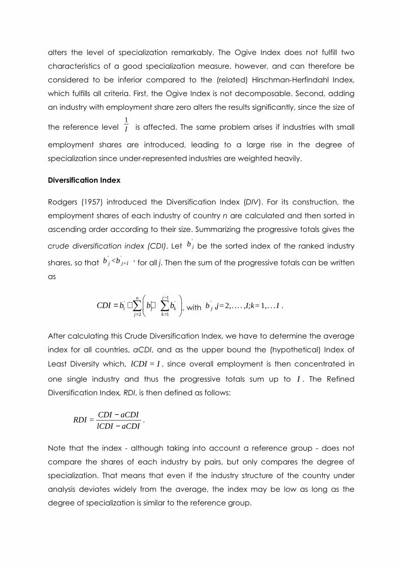
alters the level of specialization remarkably. The Ogive Index does not fulfill two
characteristics of a good specialization measure, however, and can therefore be
considered to be inferior compared to the (related) Hirschman-Herfindahl Index,
which fulfills all criteria. First, the Ogive Index is not decomposable. Second, adding
an industry with employment share zero alters the results significantly, since the size of
the reference level 1I is affected. The same problem arises if industries with small
employment shares are introduced, leading to a large rise in the degree of
specialization since under-represented industries are weighted heavily.
Diversification Index
Rodgers (1957) introduced the Diversification Index (DIV). For its construction, the
employment shares of each industry of country n are calculated and then sorted in
ascending order according to their size. Summarizing the progressive totals gives the
crude diversification index (CDI). Let b j'be the sorted index of the ranked industry
shares, so that b j' <b j+1
'‘ for all j. Then the sum of the progressive totals can be written
as
1' ' '1
2 1
jn
j kj k
CDI b b b−
= =
= + +
∑ ∑ , with b j
' ,j= 2,. .. .,I;k= 1,. . .I .
After calculating this Crude Diversification Index, we have to determine the average
index for all countries, aCDI, and as the upper bound the (hypothetical) Index of
Least Diversity which, I=lCDI , since overall employment is then concentrated in
one single industry and thus the progressive totals sum up to I . The Refined
Diversification Index, RDI, is then defined as follows:
aCDIlCDI
aCDICDI=RDI
−−
.
Note that the index - although taking into account a reference group - does not
compare the shares of each industry by pairs, but only compares the degree of
specialization. That means that even if the industry structure of the country under
analysis deviates widely from the average, the index may be low as long as the
degree of specialization is similar to the reference group.

The RDI turns negative whenever the economic structure of the reference country
group deviates from the equi-distribution of industries while the country under study
at the same time is more specialized than the reference country group, i.e.
lCDI>aCDI>CDI . For the case where the reference group has equal employment
shares in all industries while the specific country is specialized in one single industry,
the index is not defined, since then aCDI=lCDI , which would imply that the
denominator turns zero. The RDI hence only turns positive when the economic
structure of the reference country group deviates from the equi-distribution of
industries and the country under study is less specialized than the reference country
group, i.e. lCDICDI>aCDI ≥ . This implies that the RDI is an inverse measure of
specialization with the lower bound at 1. It is reached if the country under study is
characterized by an equi-proportional industry structure, i.e. lCDI=CDI . This is true
irrespective of the degree of specialization of the reference group – as long as
lCDIaCDI ≠ . The upper bound is not defined since in such a case CDI is maximized,
whereas aCDI=lCDI , turning the numerator of the RDI zero. In addition to this
deficiency, the Diversification Index is not decomposable. Moreover, adding an
industry with an employment share of zero (or even a very small industry) may lead
to a considerable change in results, since the level of lCDI is not affected as much as
the levels of CDI and aCDI. It may therefore yield results that indicate a high level of
specialization even though this is not the case in reality. The Diversification Index
fulfills the three other criteria of a good specialization measure– the Axiom of
Anonymity, the Axiom of Progressive Transfers and the Classification of industries.
Absolute Gini-Index
The Gini Index (Gini 1912 or 1921) is a common measure of income equality and
heterogeneity of economic structures. Yet it is widely applied as a relative measure
only. To our knowledge, the Gini Index has not yet been applied as an absolute
measure in the field of specialization. We introduce it in order to give a full account
of indices and to compare the different outcomes of the Absolute and the Relative
Gini Indices.
In order to calculate the Absolute Gini Index of Specialization (Abs. GINI), the relative
employment shares of the country are ranked in ascending order for the
construction of the Lorenz curve. Since the reference level is1I , the ordering of the

employment shares is the following: bi
I≥
bi − 1
I . The Lorenz curve is generated by
ordering the progressive totals of the employment shares ib on the y-axis and the
progressive totals of 1I on the x-axis and then connecting the points. Next, the 45
°
line is introduced, which is equal to the progressive totals of1I . In order to finally
determine the Gini coefficient, we define LA to be the area under the Lorenz curve.
The Gini coefficient G then is 1−2AL
I 2 . The Gini coefficient thus represents the
difference between a country’s actual distribution of employment and the equal
distribution of employment over all industries. The lower bound of the absolute Gini
Index is zero. It is reached when all industries are of equal size, i.e. 1I and hence the
Lorenz curve represents the 45°line. The upper bound of the Absolute Gini Index is
I − 1I but it converges towards one for a very large number of industries.
The Absolute is characterized by several shortcomings: First, they are not
decomposable. Second, total heterogeneity cannot simply be split up into
intersectoral and inter-industry (or similarly inter- and intraregional) heterogeneity, but
includes a third term, called transvariation (Dagum 1997), which does not have a
clear interpretation in the context of specialization. Third, the Index does not satisfy
the Axiom of Progressive Transfers, since values in the middle part of the distribution
are weighted more heavily than values at the tails of the distribution (Cowell 1995 or
Amiti 1999). Therefore e.g. a country A characterized by the economic structure
)=b;=b;=b;=(bd 432B 0.40.250.250.1: 1 should have a lower absolute specialization
level than country B with the following economic structure
)=b;=b;=b;=(bd 432B' 0.40.40.10.1: 1 ; this is not the case if the level of specialization
is calculated with the help of a Gini index. Moreover, the index is sensitive to the
splitting and merging of industries, as well as to adding industries with an
employment of zero: Merging sub-industries to one larger industry decreases the level
of specialization measured by the Gini index, which contradicts the intuition that
absolute specialization should increase when industries are merged. The
employment distribution )=b;=(bd 2C 01: 1 , for instance, would result in a lower Gini

index value than )=b;=b;=b;=(bd 432D 000.50.5: 1 , even though intuitively a
country ought to be considered more specialized if the economic structure is
represented by distribution dC rather than distribution dD. Introducing new industries
with an employment share of zero – which should not alter a good specialization
index strongly - leads to a significant increase in the level of specialization due to
changes in the reference level 1I . Therefore, the Absolute Gini Index only fulfills the
Axiom of Anonymity.
In summary, for the analysis regarding the absolute level of specialization, the
Hirschman-Herfindahl Index is not only an easily computable index but also fulfills
more criteria than all other indices presented (see Table 3). It can thus be regarded
as superior to other measures, especially if α is chosen closer to 1 in order to
counterweight the influence of large industries. Likewise, one could use the Shannon
Entropy index, but it has to be kept in mind that the index is problematic if industries
with employment shares of zero are contained in the sample. Both the Diversification
Index and the Absolute Gini Index are not only more time-consuming to calculate
but also fail to satisfy important criteria of good specialization measures.
Table 3: Criteria of Absolute Specialization Measures
Anonymity Progressive
Transfers
Decomposa
bility
Splitting/
Merging
Industries
with bi= 0
Bounds
HHI � � � � � �
SEI � � � � x �
Ogive � � x � x �
DIV � � x � x X
Abs. GINI � x x x x �
Heterogeneity Indices
Krugman Specialization Index
The Krugman Specialization Index (K) is the standard index among the specialization
measures. Basically, it is the standard error of industry shares, i.e. it calculates the
share of employment which would have to be relocated to achieve an industry
structure equivalent to the average structure of the reference group. The reference

value ib can be either one other country, as originally in Krugman (1991a), or it can
refer to the mean of all other countries, as in Midelfart-Knarvik et al. (2000) or Longhi
et al. (2004) or Palan and Schmiedeberg (2010).
∑ −I
=i
ii |bb|=K1
The Krugman Specialization Index can take values in between zero and( )
I
I 12 −. If
relative specialization is zero, the economic structure of a single country resembles
the economic structure of the reference level (i.e. the EU-average in our case). The
higher the index, the more the economic structure of one country deviates from the
reference group and the more a country is considered to be specialized. In contrast
to the absolute measures of specialization presented above, a country with a much
more equilibrated structure (and thus a lower HHI) than a highly specialized
reference country group will thus receive a high K-value, whereas a country
specialized in the same industries as the reference countries will receive a low K-
value (irrespective of the high HHI of both the country and the reference group). A
favorable property of the Krugman Specialization Index is that splitting one industry
into sub-industries will not alter the degree of specialization if the country is relatively
more specialized than the reference group in all sub-industries. On the other hand, if
the country under study is relatively more specialized in some sub-industries, while
being relatively less specialized in some other sub-industries compared to the
reference group, then merging industries would decrease the level of specialization
since patterns of over- and under-specialization cancel each other out. Adding
industries with zero or very low employment shares does not alter the level of
specialization. Hence, the Krugman Specialization Index fulfills all criteria but
decomposability.
Index of Inequality in Productive Structure
The Index of Inequality in Productive Structure (IP) was introduced by Cuadrado-
Roura et al. (1999), but variations thereof have also been employed by Haaland et
al. (1999), Landesmann (2000), and Percoco et al. (2005)
( )∑ −I
=i
ii bb=IP1
2

The IP is simply the variance of employment shares. It is similar to Krugman’s
Specialization Index, but by adding up the squared deviations of employment
shares, it gives more weight to large deviations. This can be clarified by the following
example: Let the distribution underlying the economic structure of country A be
)=b;=b;=b;=(bd 432A 0.10.20.30.4: 1 and let the economic structure of the
reference group be: )=b;=b;=b;=(bd 432R 0.20.30.40.1: 1 , the IP value in this case is
higher than for the case that the reference group would be characterized by
)=b;=b;=b;=(bd 432R' 0.30.30.20.2: 1 , even though ∑ −I
=i
ii =bb1
0.5 in both cases as
shown in Table 4:
Table 4: Heterogeneity of Employment Shares
Country
A
Reference
Group Case 1
Heterogeneity
Case 1
Reference
Group Case 2
Heterogeneity
Case 2
b1 0.4 0.1 0.3 0.2 0.2
b2 0.3 0.4 0.1 0.2 0.1
b3 0.2 0.3 0.1 0.3 0.1
b4 0.1 0.2 0.1 0.3 0.2
∑ −I
=i
ii bb1
0.6 0.6
IP 0,12 0,1
Even if the economic structure of country A does not change, the specialization level
of country A falls compared with the second reference group since the deviations in
every single industry are smaller compared with the first distribution. Thus, even if the
sum of the single distributions is the same, in the first case the larger deviation in
industry 1 outweighs smaller differences in other industries (see Table 4). This implies
that a country with a larger deviation in one single industry will be regarded as more
specialized than a country with smaller deviations in more industries. Larger industries
per se do not a lead to a bias, as long as all countries have large employment shares
in these industries. It is large absolute deviations – which, however, are more likely to
occur in larger industries – that are weighted more by this index than e.g. by the
Krugman Specialization index.

The IP can take values between zero andI − 1
I . Adding industries with very low
employment shares does not alter the level of specialization if the employment share
is low in all countries. Moreover, the Axiom of Anonymity and the Axiom of
Progressive Transfers are fulfilled. It yields problematic results if industries are split or
merged, however: Splitting an industry which the country is relatively specialized in
sub-industries leads to a decline in specialization also if the country under study is
relatively more specialized in all sub-industries than the reference group. This is due to
the fact that the employment share deviations are squared and thus adding up all
deviations before squaring gives higher values than squaring each deviation
individually and then summing up the individual deviations. If the country has lower
employment shares in some sub-industries and higher employment shares in other
sub-industries than the reference group, then merging these industries leads to a
decline of specialization in line with the Axiom of the Classification of Industries. One
further deficit of the IP is that it is not decomposable.
Relative Gini Index
The Relative Gini Index (Rel. GINI) is a common index in many fields of economics,
with many applications also in the context of industry structure and specialization.
The first to use this index in the field of specialization measurement was Hoover
(1936), who studied industrial localization. In recent years, it has been employed by
Conkling (1963), Kim (1995), Amiti (1998, 1999), Haaland et al. (1999), Brülhart (2001a),
Aiginger and Leitner (2002), Midelfart-Knarvik et al. (2000), Beine and Coulombe
(2007), Südekum (2006), Brülhart and Torstensson (2007), and Ezcurra and Pascual
(2007) in the empirical analysis of both specialization and concentration.
In order to calculate the Gini Index for a single country, the Balassa Index has to be
calculated similar to the Absolute Gini index. The only difference is that the
employment shares of every industry in the country under study are set in relation to
the employment share in the reference group instead of using the reference level
1/I. The lower bound of the Relative Gini Index is zero, since whenever the economic
structure of the country under study completely mirrors the economic structure of the
reference group, the Lorenz curve coincides with the 45°line. Its upper bound is
1− 1
I 2 , which converges towards 1 for large numbers of industries.

The Relative Gini Index is only decomposable if the range of the values taken by the
variable of interest does not overlap across subgroups of individual observations
(Cowell 1980 or Dagum 1997), so that the transvariation is zero. This is evidently not
the case in our context: different countries may well have similar degrees of
specialization in a particular industry. A further drawback of the Relative Gini Index is
that not all deviations from the economic structure of the reference group are
treated equally. This can be illustrated by the following example: Let the economic
structure of the reference group be )=b;=b;=b;=(bd 432r 0.40.30.20.1: 1 . If country
A is characterized by the economic structure )=b;=b;=b;=(bd 432A 0.40.40.10.1: 1 , it
is considered to be less specialized than if it had the economic structure
)=b;=b;=b;=(bd 432A' 0.30.30.20.2: 1 or )=b;=b;=b;=(bd 432A 0.350.250.250.15: 1'' .
Thus the more closely the smallest and largest employment shares are distributed, the
more specialized a country appears to be, even though ∑ −I
=i
ii bb1
is the same in all
three cases. Hence, the Axiom of Progressive Transfers is not satisfied. Adding
industries with an employment share of zero both at the country and at the
reference group level results in impossibility to calculate the Gini Index, since 00 is not
defined. Adding industries with negligibly small employment shares strongly increases
the level of specialization (even more than in case of the Absolute Gini Index), giving
rise to misleading conclusions. Moreover, we obtain misleading results when merging
industries. Since the area between the Lorenz curve and the 45°line automatically
gets smaller, the level of specialization decreases if industries are merged –
irrespective of whether if the country is over- or under-specialized in the respective
sub-industries.
Theil Index
The Theil Index (Theil 1967) builds on information theory, borrowing from Shannon
(1948). It has been implemented for the analyses of specialization and concentration
by Maasoumi (1993), Duro Moreno (2001), Brülhart and Traeger (2005) or Ezcurra and
Pascual (2007).

The Theil Index (T) is a variation of the Shannon Entropy Index, which sets all
employment shares of a country, bi , in relation to the employment shares of the
reference group, i :
∑I
=i i
i
i
i
b
b
b
b
I=T
1
ln1
Due to its decomposition qualities, the Theil Index has been used widely in the
research of income inequality (Shorrocks 1980 or 1984). This is doubtless the great
advantage of the Theil Index, since it is the only decomposable relative
specialization measure. Yet the Theil Index is not superior to other heterogeneity
indices in all aspects: Adding an industry with an employment share of zero would
lead to an undefined index. A problem arises for the definition of the upper bound:
Perfect relative specialization implies that the country is completely specialized in
one industry while i,I
=bi ∀1, but in that case, the Theil Index is equal to negative
infinity; yet it converges towards IIln if we allow for the existence of negligible small
industries. If the economic structures of the country and the reference group are
identical, then the Theil Index is zero. This however is not the lower bound of this
index: If the country is under-specialized in more industries than it is over-specialized
in relation to the reference group, then the Theil Index turns negative.
The largest difficulty with respect to the Theil Index is that it may yield distorted results,
since not all deviations of a country’s economic structure from the reference level
are weighted equally. This can lead to an erroneous perception of specialization
levels and consequently to misleading conclusions. To illustrate the problem, take the
following example: Country A has the employment distribution
)=b;=b;=b;=(bd 432A 0.20.20.10.5: 1 and the employment distribution of the
reference group is )=b;=b;=b;=(bd 432R 0.050.20.250.5: 1 . Note that the
employment shares in industry 1 and 3 are identical; there are only deviations in
industries 2 and 4. The Theil Index gives a value of 1.29 in this case. If the distribution of
country A changes to )=b;=b;=b;=(bd 432'A 0.20.40.30.1: 1 and the economic
structure of the norm changes such that )=b;=b;=b;=(bd 432'R 0.350.40.150.1: 1 ,
then again industries 1 and 3 are characterized by identical employment shares in
country A and in the reference country group. The deviations in industries 2 and 4 are

identical as in the other case – each is 0.15. But for the latter distributions the Theil
Index is only 0.39. So, even though the deviations from the economic structures are
identical, the index values obtained vary. In addition, the Theil Index leads to
irrational results if industries are split into sub-industries because specialization rises
under all circumstances whereas a merger of industries leads to de-specialization
(irrespective whether the country under study is more specialized in all or only some
sub-industries).
To summarize, the Index of Inequality in Productive Structure should not be used as a
measure of specialization, since it has disadvantages compared to the closely
related Krugman Specialization Index. The Relative Gini Index is widely used in the
empirical analysis of specialization patterns, yet both the Krugman Specialization
Index and the Theil Index seem superior. Whether the Krugman Specialization Index
or the Theil Index is more suitable for analysis depends on the research question and
the aims of empirical analysis. If the focus is on differences between interregional
and international specialization patterns, then the Theil Index is better suited since this
index is the only one that possesses the decomposability property. This could be of
special interest if studying the economic development of countries with large
interregional differences such as Italy or Spain, where large interregional disparities
within the respective countries are found. In cases where the analysis focuses on the
development of economic structures over time, in which the appropriate estimation
of specialization levels is important, the Krugman Specialization Index must be
recommended since it is the only measure that possesses the criterion of the
classification of industries.
Table 5: Criteria of Relative Specialization Measures
Anonymity Progressive
Transfers
Decompos
ability
Splitting/
Merging
Industries
with bi= 0
Bounds
K � � X � � �
IP � � X X � �
T � � � X x X
Rel. GINI � x x x x �

Sensitivity Analysis: Specialization of European Countries
Data and Variables
In the following section we present a specialization ranking of 24 European countries
in the year 2005 in order to illustrate that the indices described above produce quite
different results, according to their characteristics. We use employment data from
the KLEMS data base (see Timmer et al. 2007), which provides data collected from
the national accounts of the EU countries. We include 51 industries, covering the
agricultural, manufacturing and service sectors. The variable we use is annual
employment in full-time equivalents, a common measure for industry structure.
Similarly, we could focus on e.g. value added - a variable which is less prone to
productivity biases, but might be susceptible to measurement errors and exchange
rate biases. But as our focus is the measurement methods rather than the
specialization itself, the choice of variables is of minor importance. However, it should
be born in mind that also this choice will influence the results.
Due to the different domains of definition of the indices, the index values cannot be
compared directly, but only the rankings obtained by calculating the indices for all
countries. In Table 6 and Table 7 we present the rankings of the absolute and relative
specialization measures, respectively, with the least specialized countries on the top.
For the comparison we apply Spearman correlation coefficients in order to learn
about (dis-)similarities of the indices.

Table 6: Country Rankings for Absolute Specialization Indices
Absolute Specialization
Rank Hirschman-
Herfindahl Index*
Shannon Entropy
Index
Diversification
Index
Absolute Gini
Index
1 CZ 0.044 EST 2.583 CZ -0.065 CZ 0.471
2 EST 0.045 CZ 2.559 SVN -0.023 EST 0.500
3 IT 0.046 SVN 2.534 SVK -0.016 IT 0.500
4 MLT 0.047 MLT 2.527 DE -0.006 DE 0.502
5 SVK 0.047 SVK 2.526 IT 0.006 HUN 0.513
6 SVN 0.048 HUN 2.487 EST 0.010 SWE 0.524
7 DE 0.049 IT 2.485 HUN 0.013 FIN 0.538
8 HUN 0.049 SWE 2.462 MLT 0.017 AUT 0.540
9 AUT 0.051 DE 2.459 SWE 0.059 IRL 0.545
10 FIN 0.055 LVA 2.453 AUT 0.068 ESP 0.548
11 LVA 0.055 FIN 2.420 FIN 0.076 LVA 0.548
12 FRA 0.057 IRL 2.411 IRL 0.096 FRA 0.550
13 IRL 0.057 CYP 2.390 FRA 0.105 DK 0.553
14 SWE 0.057 LTU 2.378 UK 0.119 NLD 0.555
15 UK 0.058 PRT 2.372 ESP 0.124 UK 0.555
16 ESP 0.058 BEL 2.368 NLD 0.129 BEL 0.559
17 GRC 0.060 DK 2.361 DK 0.130 SVN 0.569
18 CYP 0.061 UK 2.356 BEL 0.136 SVK 0.571
19 NLD 0.061 AUT 2.356 LVA 0.139 PRT 0.581
20 DK 0.062 POL 2.354 POL 0.153 GRC 0.584
21 PRT 0.062 ESP 2.352 GRC 0.176 MLT 0.585
22 BEL 0.062 GRC 2.344 PRT 0.194 LTU 0.593
23 LTU 0.064 NLD 2.337 LTU 0.218 CYP 0.594
24 POL 0.081 FRA 2.330 CYP 0.232 POL 0.640
* The ranking is identical for the HHI and the Ogive Index, but with different index values. The Ogive
Index therefore is not listed separately. Source: EU KLEMS database, March 2008.

Table 7: Country Rankings for Relative Specialization Indices
Ran
k
Krugman
Specialization
Index
Index of Inequality
in Productive
Structure
Theil Index Relative Gini
Index
1 AUT 0.148 AUT .0011 ESP -0.049 CZ 0.169
2 FRA 0.170 FRA .0020 FRA -0.007 DE 0.181
3 DE 0.212 DE .0025 AUT -0.002 HUN 0.207
4 UK 0.256 CZ .0038 BEL 0.027 SVK 0.212
5 ESP 0.257 IT .0039 UK 0.044 IT 0.224
6 NLD 0.260 UK .0047 NLD 0.103 SVN 0.242
7 IT 0.262 NLD .0047 DE 0.104 FRA 0.246
8 FIN 0.299 HUN .0047 POL 0.207 AUT 0.271
9 CZ 0.299 SVK .0049 PRT 0.236 SWE 0.278
10 HUN 0.301 FIN .0054 IT 0.238 NLD 0.281
11 DK 0.316 MLT .0057 DK 0.259 ESP 0.282
12 IRL 0.324 ESP .0059 LVA 0.276 UK 0.283
13 SVK 0.329 IRL .0060 SVN 0.288 MLT 0.290
14 SVN 0.343 SVN .0069 HUN 0.299 IRL 0.305
15 BEL 0.345 GRC .0075 FIN 0.300 FIN 0.306
16 GRC 0.345 BEL .0083 SWE 0.305 BEL 0.320
17 SWE 0.376 DK .0089 GRC 0.310 EST 0.325
18 MLT 0.389 SWE .0098 CZ 0.315 POL 0.333
19 PRT 0.438 PRT .0110 SVK 0.354 DK 0.344
20 LVA 0.465 LVA .0112 LTU 0.418 GRC 0.356
21 EST 0.469 EST .0124 IRL 0.525 LVA 0.426
22 POL 0.473 LTU .0175 EST 0.729 PRT 0.441
23 LTU 0.516 CYP .0177 MLT 0.729 LTU 0.468
24 CYP 0.553 POL .0338 CYP 0.794 CYP 0.514
Source: EU KLEMS database, March 2008.

Results
The difference between the absolute the specialization measures and the
heterogeneity (relative specialization) indices are visible at first glance (see Table 8).
We have argued above that one cannot compare absolute specialization indices
with heterogeneity indices, simply because the focus of both concepts is totally
different. To give an example: While Estonia is listed in the top positions of the
absolute specialization rankings, it is at the end of the rankings in terms of relative
specialization, i.e. the measures indicate a low degree of absolute specialization, but
a high degree of relative specialization compared to the European average industry
structure. The general differences among the two groups of indices become more
evident when calculating the correlation coefficients regarding the country
specialization ranking. From Table 8 it becomes obvious that absolute indices
measure different concepts of specialization than relative indices. It thus comes as
no surprise that in several cases the outcome of absolute and relative indices is even
negative. It is thus more remarkable that both the Relative Gini Index and the Index
of Inequality of Production Structure are highly positively correlated with all absolute
specialization index but the Shannon Entropy Index. In this respect it is also quite
remarkable, that the absolute and Relative Gini Indices are characterized by a
coefficient of 0.587 only. This again emphasizes the different focus of absolute and
relative specialization indices, respectively.
Table 8: Correlation between Absolute and Relative Indices
HHI SEI DIV Abs. G
K .291 -.268 .432 .518
IP .522 -.030 .595 .501
T -.284 -.624 -.105 .110
Rel. G .664 .335 .863 .587
More interesting are the differences within the two groups. Within the group of
absolute specialization measures we identify notable differences in the results (see
Table 9): Even though the HHI and SEI are constructed in a similar way and differ from
each other mainly by different weighting schemes, they produce rankings which are
not more similar than the result produced by the ranking-based Diversification Index.
Taking a ranking difference of four or more ranks as a criterion, it is notable that only

about half of the countries are ranked similarly by the three measures. The least
congruency is found between the Absolute Gini Index and all other measures –
above all with the Shannon Entropy Index.
Table 9: Correlation between Absolute Measures
HHI SEI DIV Abs. G
HHI 1.000
SEI .741 1.000
DIV .885 .691 1.000
Abs. G .619 .376 .641 1.000
Regarding the group of relative specialization measures, the most similar results are
given by the Krugman Index and the Index of Inequality in Productive Structure (see
Table 10). This is not unexpected as these two indices are very similar to one another.
Seven out of 24 countries are placed at the same position in the rankings (while only
three countries on average are assigned the same rank by two indices). Interestingly,
the best accordance is found at both ends of the ranking, i.e. the ranking of the least
and most specialized countries (relative to the EU average) are nearly identical,
while in the middle ranks the differences increase.
Table 10: Correlation between Relative Measures
K IP T Rel. G
K 1.000
IP .912 1.000
T .640 .414 1.000
Rel. G .688 .805 .240 1.000
The results attained by the Theil Index in contrast differ strongly from the other
rankings (see Table 10). The results of the Relative Gini Index and the Index of
Inequality in Production Structure are highly correlated. This could be due to the fact
that both give more weight to large deviations than the other Indices.
For illustration purposes we compare the Czech Republic and Malta: Both countries
are strongly diversified (i.e. the values for absolute specialization are rather low), but

while the Czech Republic seems to have an industry structure similar to the EU
average, the specialization pattern of Malta evidently differs from the average EU
structure. This can be seen from the fact that Malta is ranked lower than Czech
Republic in all rankings. Still, there are large differences in the ranks the countries are
given by the relative specialization indices: According to the Relative Gini and IP
Indices, the Czech Republic is one of the countries which are most similar to the
average, and thus in the fore of the rankings, while the Krugman and Theil Indices,
which give less weight to large industries, place the country in the middle of the
ranking. Regarding the Theil Index, the outstanding result of Poland is worth
mentioning. Whereas this country ranks very low in all other indices due to its
exposure to the agricultural and food sector, the results give a much higher
specialization value if calculated with the Theil Index. This confirms that the Theil
Index is indeed giving more weight to one-sector-specialization in comparison to all
other indices.
Comparing the correlation coefficients of the comparison within the both index
groups (Table 9 and Table 10) with the values in Table 8, it is remarkable that the
differences within the groups are partly even larger than between absolute and
relative specialization indices – which we have said to be totally different in their
concept and focus.
Conclusion
To summarize, we find that results differ widely according to which measure is used.
As expected, results from measures of absolute specialization cannot be compared
to indices of relative specialization, since they follow two distinct concepts of
specialization. But even within both groups the indices differ from each other due to
different construction and weighting schemes. As a result, the rankings do not
consistently match. While the Krugman Specialization Index and the Index of
Inequality in Productive Structure, which are constructed similarly, are concordant in
a large number of cases, all other comparisons show only occasional congruence.
Hence, the pictures these rankings draw are somewhat arbitrary.
A general problem of specialization indices is that they are only able to give a very
aggregate picture and thus convey only a limited understanding of the
development of the economic structure of a country, since they give no information
about the underlying developments, i.e. in which industries countries are specializing.

None of the presented aggregate indices is able to indicate which industries drive
specialization patterns in a country.
Moreover, all indices presented above focus on the distribution of employment
across industries only and do not to account for inter-industry linkages. Due to the
quite limited availability of consistent input-output data over a long time horizon, the
application of more sophisticated measures of specialization is hard to accomplish in
empirical studies.
Literature
Acar, W. and K. Sankaran (1999), The Myth of the Unique Decomposability:
Specializing the Herfindahl and Entropy Measures? in: Strategic Management
Journal, Vol. 20, 969-975.
Aiginger, K. and St. Davies (2004), Industrial specialization and geographic
concentration: two sides of the same coin? Not for the European Union, in: Journal of
Applied Economics, vol. 12, 231-248.
Aiginger, K. and W. Leitner (2002), Regional Concentration in the United States and
Europe: Who Follows Whom? in: Weltwirtschaftliches Archiv, vol. 138, 652-679.
Aiginger, K. and M. Pfaffermayr (2004), The Single Market and Geographic
Concentration in Europe, in: Review of International Economics, vol. 12, 1-11.
Amiti, M. (1998), New Trade Theories and Industrial Location in the EU: A Survey of
Evidence, in: Oxford Economic Review, vol. 14, 45-53.
Amiti, M. (1999), Specialisation Patterns in Europe, in: Review of World Economics, vol.
573-593.
Atkinson, A.B. (1970), On the Measurement of Inequality, in: Journal of Economic
Theory, vol. 2, 244-263.
Attaran, M. and M. Zwick (1987), Entropy and Other Measures of Industrial
Diversification, in: Quarterly Journal of Business and Economics, vol. 26, 17-35.
Bahl, R.W.; Firestine, R. and D. Phares (1971), Industrial Diversity in Urban Areas:
Alternative Measures and Intermetropolitan Comparisons, in: Economic Geography,
vol. 47, 414-425.
Beine, M. and S. Coulombe (2007), Economic integration and the diversification of
regional exports: evidence from the Canadian-U.S. Free Trade Agreement, in:
Journal of Economic Geography, vol. 7, 93-111.
Bourguignon, F. (1979), Decomposable income inequality measures, in:
Econometrica, vol. 47, 901-920.
Brown, D.J. and J. Pheasant (1985), A Sharpe Portfolio Approach to Regional
Economic Analysis, in: Journal of Regional Science, vol. 25, 51-63.
Brülhart, M. (2001a), Growing alike or growing apart? Industrial specialisation of EU
Countries, in: C. Wyplosz (ed.), The Impact of EMU on Europe and the Developing
Countries, Oxford University Press.
Brülhart, M. and J. Torstensson (2007), Regional Integration, Scale Economies and
Industry Location in the European Union, in: Jovanovic, M.N. (ed.), Economic
Integration and Spatial Location of Firms and Industries, Vol. I, Cheltenham.
Brülhart, M. and R. Traeger (2005), An account of geographic concentration patterns
in Europe, in: Regional Science and Urban Economics, vol. 35, 597-624.
Chisholm, M. (1968), Rural Settlement and Land Use. An Essay in Location, Chicago.
Chisholm, M. and J. Oeppen (1973), The Changing Pattern of Employment. Regional
Specialisation and Industrial Location in Britain, London.
Combes, P.-P. and H.G. Overman (2004), The spatial distribution of economic
activities in the European Union, in: Henderson, J.V. and J.F. Thisse (eds), Handbook
of Regional and Urban Economics, ed. 1, vol. 4, chapter 64, 2845-2909, North
Holland.
Conkling, E.C. (1963), South Wales: A Case Study in Industrial Diversification, in:
Economic Geography, vol. 39, 258-272.
Conroy, M.E. (1975b), The concept and measurement of regional industrial
diversification, in: Southern Economic Journal, vol. 41, 492-505.
Cowell, F. A. (1980), On the structure of additive inequality measures, in: Review of
Economic Studies, vol. 47, 521.31.
Cowell, F.A. (1995), Measuring Inequality, London.
Cowell, F. A. (2000). Measurement of inequality. in Atkinson, A.B. and F. Bourguignon
(eds.), Handbook of Income Distribution, 87-166, Amsterdam:.

Cuadrado-Roura, J.R.; Garcia-Greciano, B. and J.L. Raymond (1999), Regional
Convergence in Productivity and Productive Structure: The Spanish Case, in:
International Regional Science Review, vol. 22, 35-53.
Dagum, C. (1997), A New Approach to the Decomposition of the Gini Income
Inequality Ration, in: Empirical Economics, vol. 22, 515-531.
Dalton, H. (1920), The Measurement of Inequality of Incomes, in: The Economic
Journal, vol. 30, 348-361.
Davis, D.R. (1998), The Home Market, Trade, and Industrial Structure, in: American
Economic Review, vol. 88, 1264-1276.
Devereux, M.P.; Griffith, R. and H. Simspon (2004), The geographic distribution of
production activity in the UK, in: Regional Science and Urban Economics, vol. 34, 533-
564.
Duro Moreno, J.A. (2001), Cross-country inequalities in aggregate welfare: some
evidence, in: Applied Economic Letters, vol. 8, 403-406.
Ellison, G. and Glaeser, E. (1997), Geographic Concentration in US Manufacturing
Industry: a Dartboard Approach, in: Journal of Political Economy, vol. 105, 889-927.
Ezcurra, R. and P. Pascual (2007), Spatial Disparities in Productivity in Central and
Eastern Europe, in: Eastern European Economics, vol. 45, 5-32.
Florence, P.S. (1948), Investment, Location, and Size of Plant, Cambridge.
Gini, C. (1912). Variabilità e mutabilità, Reprinted in: Pizetti, E. and T. Salveini (eds.)
Memorie di metodologica statistica, 1955, Rome.
Gini, C. (1921), Measurement of Inequality of Incomes, in: The Economic Journal, vol.
31, 124 -126.
Gratton, C. (1979), Industrial Diversification in New Towns, in: Urban Studies, vol. 16,
157-164.
Haaland, J.I.; Kind, H.J.; Midelfart-Knarvik, K.H. and J. Torstensson (1999), What
determines the economic geography of Europe, CEPR Discussion Paper, No. 2072.

Hackbart, M.W. and D.A. Anderson (1975), On Measuring Economic Diversification,
in: Land Economics, vol. 51, 374-378.
Hall, M. and N. Tideman (1967), Measures of Concentration, in: Journal of the
American Statistical Association, vol. 62, 162-168.
Hannah, L.and Kay, J. A. (1977), Concentration in Modern Industry. Theory,
Measurement and the UK Experience, London.
Herfindahl, O. C. (1950). Concentration in the Steel Industry. Ph. D. thesis, Columbia
University.
Hirschman, A.O. (1964), The Paternity of an Index, in: The American Economic
Review, vol. 54, 761-762.
Hoover, E.M. (1936), The Measurement of Industrial Localization, in: The Review of
Economics and Statistics, vol. 18, 162-171
Jackson, R.W. (1984), An evaluation of alternative measures of regional
diversification, in: Regional Studies, vol. 18, 103-112.
Keeble, D.E. and D.P. Hauser (1971), Spatial analysis of manufacturing growth in outer
South-East England 1960-1967, in: Regional Studies, vol. 5, 229-262.
Kim, S. (1995), Expansion of markets and the geographic distribution of economic
activities: the trends in US regional manufacturing structure 1860-1987, in: Quarterly
Journal of Economics, vol. 10, 881-908.
Kolm, S.C. (1969), The optimal production of social justice, in Margolis, J. and H.
Guitton (eds.), Public Economics, 145-200. London.
Krugman, P. (1991a), Geography and Trade, MIT Press.
Krugman, P. (1991b), Increasing returns and economic geography, in: Journal of
Political Economy, vol. 99, 183-199.
Landesmann, M. (2000), Structural change in the Transition Economies 1989-1999, in:
Economic Survey of Europe, vol. 2, 95-123.
Longhi, S.; Nijkamp, P and I Traistaru (2004), Economic Integration and Regional
Structural Change in a Wider Europe: Evidence from New EU and Accession

Countries, in: Journal for Institutional Innovation, Development & Transition, vol. 8, 48-
55.
Maasoumi, E. (1993), A compendium to information theory in economics and
econometrics, in: Econometric reviews, vol. 12, 137-181.
Maurel, F. and Sédillot, B. (1999), A measure of the geographic concentration in
French manufacturing industries, in: Regional Science and Urban Economics, vol. 29,
575-604.
Midelfart-Knarvik, K., Overman, H.G.; Redding, S.J. and A.J. Venables (2000), The
Location of European industry, in: European Commission (eds.), European integration
and the functioning of product market, Brussels, 213-270.
Palan, N. and C. Schmiedeberg (2010), Structural Convergence of European
Countries, in: Structural Change and Economic Dynamics, vol. 21, 85-100.
Percoco, M.; Dall’Erba, S. and G. Hewings (2005), Structural Convergence of the
National Economies of Europe, MPRA Paper, No. 1380.
Rodgers, A. (1957), Some aspects of industrial diversification in the United States, in:
Economic Geography, vol. 33, 16-30.
Rothschild, M. and J. Stiglitz (1970), Increasing Risk I, in: Journal of Economic Theory,
vol. 2, 225-243.
Sapir, A. (1996), The Effects of Europe’s Internal Market Program on Production and
Trade: A First Assessment, in: Weltwirtschaftliches Archiv, vol. 132, 457-475.
Scherer, F.M. (1990), Industrial market structure and economic performance, 3rd ed.,
Boston.
Sen, A. (1973), On Economic Inequality, New York.
Shannon, C. E. (1948), A mathematical theory of communication, in: The Bell System
Technical Journal, vol. 27, 379-423, 623-656.
Shorrocks, A.F. (1980), The class of additively decomposable inequality measures, in:
Econometrica, vol. 48, 613-625.

Shorrocks, A.F. (1984), Inequality decomposition by population subgroups, in:
Econometrica, vol. 52, 1369-1385.
Siegel, P.B.; Johnson, T.G. and J. Alwang (1995), Regional Economic Diversity and
Diversification, in: Growth and Change, vol. 26, 261-284
Smith, S.M. and C.M. Gibson (1988), Industrial Diversification in Nonmetropolitan
Counties and Its Effect on Economic Stability, in: Western Journal of Agricultural
Economics, vol. 13, 193-201.
Storper, M.; Chen, Y. and F. De Paolis (2002), Trade and the location of industries in
the OECD and European Union, in: Journal of Economic Geography, vol. 2, 73-107.
Südekum, J. (2006), Concentration and Specialisation Trends in Germany since Re-
Unification, in: Regional Studies, vol. 40, 861-873.
Tauer, L.W. (1992), Diversification of production activities across individual states, in:
Journal of Production Agriculture, vol. 5, 210-214.
Theil, H. (1967), Economics and Information Theory, North Holland.
Timmer, M., O'Mahony, M. and B. van Ark (2007), The EU KLEMS Growth and
Productivity Accounts: An Overview, University of Groningen and University of
Birmingham.
Tirole, J. (1988), The Theory of Industrial Organization. Cambridge, Mass.
Tress, R. C. (1938), Unemployment and the diversification of industry, in: The
Manchester School, vol. 9, 140-152.
Wasylenko, M.J. and R.A. Erickson (1978), “On Measuring Economic Diversification”:
Comment, in: Land Economics, Vol. 54, 106-109.
Waterson, M. (1984): The profitability-concentration relation: market power or
efficiemcy?, in: Journal of Industrial Economics, vol.32, 435-50.