measurement of ion recombination correction …s thesis, 30hp emma hedin sept 2008-jan 2009...
TRANSCRIPT

Master's Thesis, 30hp
Emma Hedin
sept 2008-jan 2009
Measurement of ion recombination
correction factors for plane parallel
ionization chambers
Supervisors:
Sean Geoghegan
Royal Perth Hospital, University of Western Australia School of Physics
Mats Isaksson
University of Gothenburg Department of Radiation Physics

Abstract
The work presented focuses on the measurement of Ja�e plots and determination of
ion recombination factors for plane parallel ionisation chambers used in pulsed electron
beams. The ability to measure the Ja�e plots accurately is useful when commisioning a
new chamber and the ion recombination correction factor needs to be known when the
chamber is calibrated in a beam quality di�erent from the user beam.
In this study the ion recombination factor is measured and Ja�e plots are produced
for three di�erent plane parallel chambers. A Roos chamber type 34001 (PTW Freiburg),
a plane parallel NACP chamber type -02 (Scanditronix) and a plane parallel Pitman
chamber (631). Experimental results are presented in form of Ja�e plots, as well as the
ion recombination correction factor, determined both from Ja�e plots and by means of
the two voltage method as recommended in IAEA TRS-398.
The report also presents results dealing with the measurement technique and experi-
mental setup. Drift, leakage and polarity e�ect are discussed. The methods of statistical
analysis are brought up and discussion is made regarding the validity of the statistical
analysis.
The measurements were performed on an Elekta linear accelerator at Perth Radiation
Oncology, Wembley, Perth WA. Energies between 6 and 15 MeV were used with doses per
pulse below 0.02 cGy per pulse.
The project goal was to measure the ion recombination correction factor and produce
a Ja�e plot for a plane parallell Pitman chamber that during various other measurements
have shown discrepancy from other chambers. In the goal was also included measurment
of the ion recombination factor and Ja�e plot for a plane parallel Roos chamber and a
plane parallel NACP chamber to allow for a comparison to be made between chambers.
The Pitman chamber was found to have a deviation from linearity of the Ja�e plot at
lower voltages than the other chambers.

Contents
1 Introduction 3
2 Theory 4
2.1 Ion Recombination . . . . . . . . . . . . . . . . . . . . . . . . . . . . . . . . . . . . . . 4
2.1.1 General and initial recombination . . . . . . . . . . . . . . . . . . . . . . . . . . 4
2.1.2 Boag's Theory . . . . . . . . . . . . . . . . . . . . . . . . . . . . . . . . . . . . 4
2.1.3 Derivation of the standard two-voltage method . . . . . . . . . . . . . . . . . . 5
2.1.4 Ja�e diagram . . . . . . . . . . . . . . . . . . . . . . . . . . . . . . . . . . . . . 5
3 Materials and Methods 6
3.1 Accuracy . . . . . . . . . . . . . . . . . . . . . . . . . . . . . . . . . . . . . . . . . . . 6
3.1.1 Stabilisation of the electrometer . . . . . . . . . . . . . . . . . . . . . . . . . . 6
3.1.2 Correction for drift . . . . . . . . . . . . . . . . . . . . . . . . . . . . . . . . . . 8
3.1.3 Polarity e�ect . . . . . . . . . . . . . . . . . . . . . . . . . . . . . . . . . . . . . 9
3.2 Statistics . . . . . . . . . . . . . . . . . . . . . . . . . . . . . . . . . . . . . . . . . . . 9
3.2.1 Error Bars . . . . . . . . . . . . . . . . . . . . . . . . . . . . . . . . . . . . . . 10
3.2.2 Linear Regression . . . . . . . . . . . . . . . . . . . . . . . . . . . . . . . . . . . 10
3.3 Method for estimating the error associated with using a linear model in non-linear Ja�e
plots . . . . . . . . . . . . . . . . . . . . . . . . . . . . . . . . . . . . . . . . . . . . . . 11
4 Results and Discussion 12
4.1 Accuracy . . . . . . . . . . . . . . . . . . . . . . . . . . . . . . . . . . . . . . . . . . . 12
4.1.1 Drift . . . . . . . . . . . . . . . . . . . . . . . . . . . . . . . . . . . . . . . . . . 12
4.1.2 Polarity e�ect . . . . . . . . . . . . . . . . . . . . . . . . . . . . . . . . . . . . . 14
4.1.3 Leakage . . . . . . . . . . . . . . . . . . . . . . . . . . . . . . . . . . . . . . . . 18
4.2 Statistical analysis . . . . . . . . . . . . . . . . . . . . . . . . . . . . . . . . . . . . . . 20
4.3 Non-linear Ja�e plots . . . . . . . . . . . . . . . . . . . . . . . . . . . . . . . . . . . . . 22
4.3.1 Ion recombination correction factors . . . . . . . . . . . . . . . . . . . . . . . . 25
4.3.2 Linear model used for non-linear Ja�e plots . . . . . . . . . . . . . . . . . . . . 28
4.4 Reproducibility of the measurement . . . . . . . . . . . . . . . . . . . . . . . . . . . . 30
4.5 Energy dependence . . . . . . . . . . . . . . . . . . . . . . . . . . . . . . . . . . . . . . 32
4.5.1 Varying depth for 15MeV . . . . . . . . . . . . . . . . . . . . . . . . . . . . . . 34
4.6 Dose Per Pulse Dependence . . . . . . . . . . . . . . . . . . . . . . . . . . . . . . . . . 38
5 Concluding Remarks 40
Acknowledgement 42
References 43
Appendix 44
5.0.1 The t-distribution . . . . . . . . . . . . . . . . . . . . . . . . . . . . . . . . . . 44
5.0.2 Cochrans theorem . . . . . . . . . . . . . . . . . . . . . . . . . . . . . . . . . . 44
5.0.3 Subgroups . . . . . . . . . . . . . . . . . . . . . . . . . . . . . . . . . . . . . . . 44

Emma Hedin
1 Introduction
When measuring absorbed dose with an ionisation chamber several corrections need to be
made to ensure that the measurement of absorbed dose gives the same result regardless of
operational conditions such as radiation quality and doserate. The International Atomic En-
ergy Agency has published a dosimetry protocol to be used for dose determination in external
radiation therapy; IAEA TRS-398. This protocol de�nes all di�erent correction factors needed
to achieve a clinically relevant accuracy of the measurements of absorbed dose. One of the
correction factors is the ion recombination factor ks, which corrects for incomplete charge
collection at an electrode due to ion recombination in the gas cavity.
The ion recombination correction factor de�ned in IAEA TRS-398 is assumed to be de-
terminable by the two-voltage method. When using this method one has to suppose that
the relationship between the reciprocal of the chamber response and the reciprocal of the po-
larising voltage is linear. In other words, the user is assuming that the chamber response is
consistent with the theory of Boag, which approximately yields a straight line in a Ja�é plot
produced for doses per pulse less than 0.1 cGy/pulse [1]. The two-voltage method is derived
from the Boag theory. However, for certain chambers and certain voltage regions the rela-
tion may be described by a more complex non-linear curve. In the clinic this deviation from
linearity may not be signi�cant, however it may be of importance in high precision radiation
dosimetry practiced at standards laboratories. In the clinic the ion recombination correction
factor determined is further assumed, within an acceptable uncertainty, to be independent of
dose per pulse and radiation quality, allowing measurements to be made at di�erent locations
in the radiation �eld using the same correction factor.
Several authors have investigated the dependence of ks on radiation type. Bruggmoser
et al. (2007) [2] and Havercroft et al. (1993) [3] report no dependence of ks on beam energy.
Several authors have also measured the dose per pulse dependency of the ion recombination
correction factor. Bruggmoser et al. [2] and Burns & McEwen [4] have for example done
measurements for doses per pulse in the order of 1 mGy/pulse.
The ion recombination e�ect will cause a change in the typical charge measured in a
radiotherapy context in the order of 0.2%. To be able to measure the ion recombination e�ect
accurately care has to be taken to account for several in�uences. The knowledge of error
propagation when calculating the correction factor from raw data is necessary for minimizing
the uncertainty in the determined ion recombination correction factor. The aim of this study
was partly to produce Ja�e plots for three di�erent chambers and determine the error that
is associated with the way the ion recombination correction factor is determined and used in
the clinic. The study also aims to compare di�erent methods for determination of the ion
recombination correction factor and to compare the results from the di�erent chambers.
� 3 �

Emma Hedin
2 Theory
2.1 Ion Recombination
The method for determining ion recombination correction factors in pulsed beams according
to IAEA TRS-398 is based on the Boag Theory. The user only needs to con�rm that the
reciprocal of the chamber response linearly depends on the reciprocal of the chamber voltage
in the voltage region in which the chamber is going to be used and then use Equation 1 which
is from IAEA TRS-398 [5]. The chamber response is to be measured for two di�erent voltages;
the usual voltage and a lower voltage. The ratio between the two voltages must be of certain
integer value. A table provides the coe�cients a0, a1 and a2 of the second order polynomial
in Equation 1
ks = a0 + a1M1
M2+ a2
(M1
M2
)2
(1)
where M1 and M2 are the chamber readings at user voltage and at the lower voltage re-
spectively, ks is the recombination correction factor de�ned in TRS-398. Derivation of this
method, called the standard two-voltage method is given in section 2.1.3.
2.1.1 General and initial recombination
The total e�ect of ion recombination is a combination of initial and general recombination.
However Burns and McEwen (1998) [4] states that; "It is well established that the component
of initial recombination also varies approximately linearly in reciprocal current against recip-
rocal voltage", which is the reason to why the total recombination correction factor ks can be
determined by models assuming linearity between the reciprocal current and the reciprocal
voltage as stated in Section 2.1.4. It should also be understood that the two voltage method
corrects for the total recombination e�ect accurately because of this.
2.1.2 Boag's Theory
Boag's theory of ion recombination in pulsed beams provides a relation between the correction
factor for general recombination ksgen and chamber voltage, dose per pulse and the distance
between the electrodes.
ksgen =u
ln[1 + epu−1p ]
(2)
where p is the free electron fraction and u is given by Equation 3. In Equation 3, µ is a
constant depending on the gas and d is the distance between the electrodes in a plane parallell
chamber. The polarising voltage is designated V and q is the amount of charge liberated per
volume of air per pulse.
u =µd2q
V(3)
� 4 �

Emma Hedin
Clinically relevant �gures of the di�erent quantities yields a small u. Di Martino et al. [1]
showed that Equation 2 can be expanded with a �rst order Taylor expansion:
ksgen ≈u
ln(1 + u). (4)
2.1.3 Derivation of the standard two-voltage method
Suppose that:
ks =qreleasedqcollected
=Ms
M(5)
In Equation 5, Ms is the true reading of the chamber and M is the actual reading of the
chamber achieved in practice. Index s stands for saturation, meaning that the true reading
is achieved when all of the charge is collected from the chamber and the saturation current
is measured. Using Equation 4 it can be shown that the ratio between the chamber response
M1 and M2 at the two di�erent voltages V1 and V2 respectively can be written as
M1
M2=
M1Ms
M2Ms
=ln(1+u1)
u1
ln(1+u2)u2
(6)
where u is de�ned by Equation 3. Equation 3 also gives the relation u2 = u1V1V2. Substituting
u2 with this expression gives
M1
M2=V1
V2
ln(1 + u1)ln[1 + V1
V2u1]
. (7)
Solving Equation 7 for u1 and inserting numbers for the chamber reading ratio and voltage
ratio respectively gives u1 to be used in Equation 4 from which ks can be obtained. Since
Equation 7 is a transcendental equation it can only be solved by numerical (or graphical)
methods. Weinhous and Meli [6] did the work of numerically solving the equation and com-
puting ks for di�erent voltage ratios and chamber reading ratios. Their results in the form of
the coe�cients of Equation 1 are used in IAEA TRS-398.
2.1.4 Ja�e diagram
A Ja�e diagram is a plot of the reciprocal of the chamber reading against the reciprocal of
the polarising voltage. Approximating Equation 4 for ks < 1.05 and consequently u < 0.1 by
expanding the nominator and letting u tend to zero yields
ksgen ≈u
ln(1 + u)≈ 1 +
u
2(8)
where u is proportional to 1V which together with section 2.1.1 leads to the conclusion that
the relation between the reciprocal of the chamber reading and the polarising voltage should
be linear for ks < 1.05.
� 5 �

Emma Hedin
3 Materials and Methods
All measurements were done on the Elekta linear accelerator M2 at Perth Radiation Oncology
except for the measurements done on the 3rd of December. On the 3rd of December the
experiment was carried out on the Elekta Linear accelerator M3 at Perth Radiation Oncology.
Three measurements were recorded for each voltage and the average of those three readings are
used to produce the diagrams in the report. Three parallel-plate chambers were investigated;
one NACP chamber type 02 (Scanditronix) serial number DEA0008703, one Roos chamber
(PTW Freiburg) serial number TW34001-1085 and a Pitman chamber serial number 631. The
chamber response of the investigated chamber was measured with a Unidos E electrometer
(PTW Freiburg) serial number T10009-90316. The reference chamber used simuntaneously
was connected to a Unidos E electrometer (PTW Freiburg) serial number T10009-90051.
3.1 Accuracy
A number of procedures were implemented to make sure that the quantity was accurately
measured. The chamber response was normalised to the response of a reference chamber
to adjust for changes in temperature, air pressure and output. The leakage current was
measured for each type of experimental setup. The electrometer was allowed to stabilise
before measurements were recorded as described in Section 3.1.1. The �rst voltage of each
experiment was repeated at the end to allow correction for drift as described in Section 3.1.2.
The readings were corrected for polarity e�ect at each voltage as described in Section 3.1.3
3.1.1 Stabilisation of the electrometer
Di�erent methods were used for ensuring that the electrometer had reached equlibrium before
measurements were recorded at a new voltage. When the Roos chamber was used with polar-
ising voltages in its linear region, the chamber responses were compared at 10 and 15 minutes
after the polarising voltage was changed. Stabilisation was asssumed to have occured when
the measurement after 10 minutes of waiting did not deviate more from the three consecutive
measurements made after 15 minutes of waiting than the 15 minutes measurements deviated
from each other. A more detailed description is that the distances A and B de�ned in Figure 1
were examined and A was assured to be less than B.
� 6 �

Emma Hedin
Figure 1: De�ning distances A and B used for determining stabilisation time for the electrometer
when a chamber was used in its linear region. Distance A was assured to be less than B before
stabilisation of the electrometer was assumed to have occured at a time t minutes after the voltage
was set.
When measurements were made on the Roos chamber with polarising voltages above
250 volts (maximum 400 volts), the stabilisation was more carefully observed. Because of
drift and a rather big instrument error at these voltages, the main trend of a gradual ap-
proach to a stabilisation value was hard to observe for some changes of voltage. However, the
chamber response ratio (MRoos/MRef ) could be observed to vary around a certain value and
was found not to vary more than twice the instrument error. This was except for the two �rst
changes in voltage when the ratio varied more and an extra period of time was spent looking
at the stabilisation to see that it was varying around a stable mean value. A stabilisation
time between 12 and 30 minutes was applied for the Roos chamber. When doing measure-
ments with the NACP chamber the stabilisation of the electrometer was carefully observed
and the ratio was not allowed to vary more than twice the instrument error. Simultaneously
the stabilisation graph was observed visually to be sure that the curve was becoming �at. A
stabilisation time between 13 and 47 minutes was applied for the NACP chamber. When mea-
surements were made with the Pitman chamber, the ratio was again not allowed to vary more
than twice the instrument error. The stabilisation curve was easy to analyse as it showed the
trend of approaching a value and �attening out for all changes of voltage. A stabilisation time
between 18 and 41 minutes was applied for the Pitman chamber. Examples of stabilisation
curves are shown in Figure 2
� 7 �

Emma Hedin
(a) (b)
Figure 2: Examples of stabilisation curves for the NACP chamber. The chamber response ratio, that
is the ratio of the NACP chamber response and the reference chamber response is plotted against time.
The time is measured from the change of voltage. In (a) the stabilisation trend is easy to observe, in
(b) the stabilisation pattern is not clear.
3.1.2 Correction for drift
The time of the recorded measurement was noted and the �rst voltage was repeated in the
end of the experiment. The drift was found to be very small and a linear time dependence of
the drift was assumed. A linear interpolation was made to approximately correct for the drift
of the system.
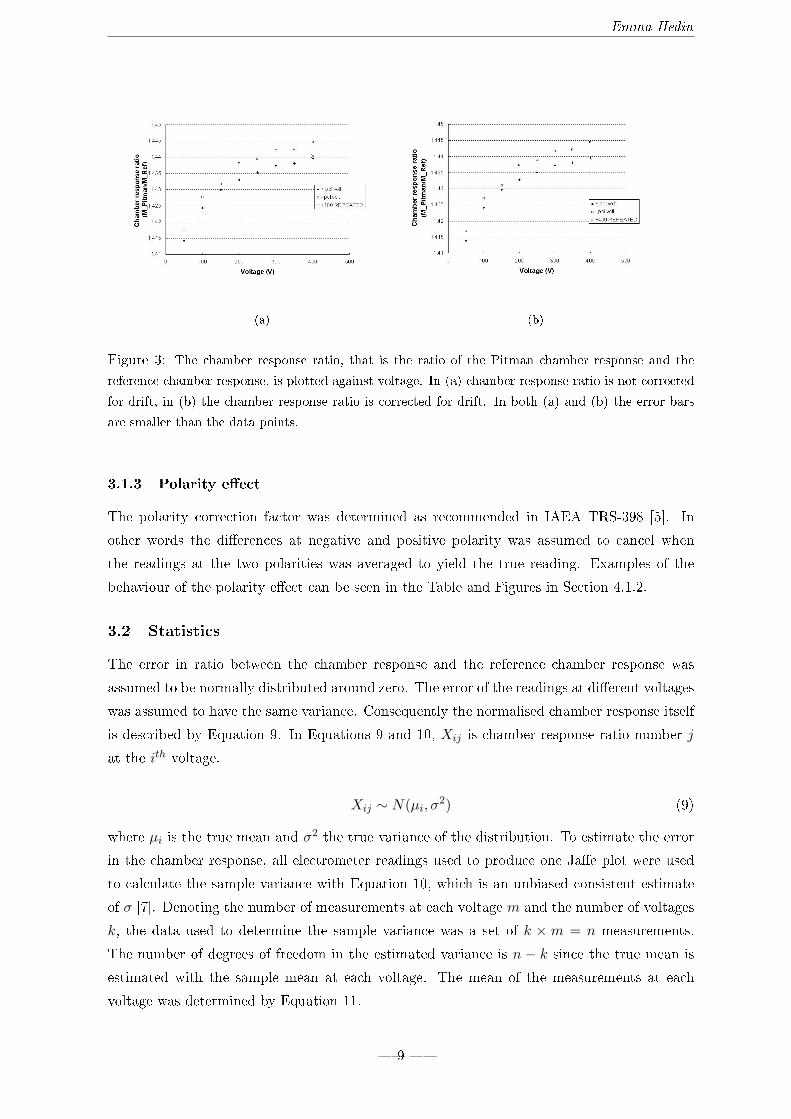
Figure 3 show an example of how the data points is shifted slightly when the drift correction
is applied. The ratio of the Pitman chamber response and the reference chamber response is
plotted against voltage, in 3(a) no drift correction is applied and in 3(b) drift correction is
applied.
� 8 �
Emma Hedin
(a) (b)
Figure 3: The chamber response ratio, that is the ratio of the Pitman chamber response and the
reference chamber response, is plotted against voltage. In (a) chamber response ratio is not corrected
for drift, in (b) the chamber response ratio is corrected for drift. In both (a) and (b) the error bars
are smaller than the data points.
3.1.3 Polarity e�ect
The polarity correction factor was determined as recommended in IAEA TRS-398 [5]. In
other words the di�erences at negative and positive polarity was assumed to cancel when
the readings at the two polarities was averaged to yield the true reading. Examples of the
behaviour of the polarity e�ect can be seen in the Table and Figures in Section 4.1.2.
3.2 Statistics
The error in ratio between the chamber response and the reference chamber response was
assumed to be normally distributed around zero. The error of the readings at di�erent voltages
was assumed to have the same variance. Consequently the normalised chamber response itself
is described by Equation 9. In Equations 9 and 10, Xij is chamber response ratio number j
at the ith voltage.
Xij ∼ N(µi, σ2) (9)
where µi is the true mean and σ2 the true variance of the distribution. To estimate the error
in the chamber response, all electrometer readings used to produce one Ja�e plot were used
to calculate the sample variance with Equation 10, which is an unbiased consistent estimate
of σ [7]. Denoting the number of measurements at each voltage m and the number of voltages
k, the data used to determine the sample variance was a set of k × m = n measurements.
The number of degrees of freedom in the estimated variance is n − k since the true mean is
estimated with the sample mean at each voltage. The mean of the measurements at each
voltage was determined by Equation 11.
� 9 �

Emma Hedin
s2 =1
n− k
k∑i=1
m∑j=1
(Xij − X̄i)2 (10)
X̄i =1m
m∑j=1
Xij (11)
3.2.1 Error Bars
The error in the chamber response was calculated from the sample variance estimated ac-
cording to Equation 10. The t-distribution was used to obtain the 95% con�dence interval
of the error of the chamber reading. Because the error in the applied polarising voltage is
not known, the error in applied voltage was assumed to be equal to 0.5% (+-0.25%) based on
prior experiences on the clinic.
To estimate the errors in the inverse normalised chamber response and the inverse nor-
malised polarising voltage the error propagation formula in Equation 13 based on work by
Arrass was used [8]. Equation 13 was also used when the error was determined for ks calcu-
lated by the means of the two voltage method. In Equation 13 the known errors are the σi:s,
Y is the quantity for which the error is being calculated and f is the function which yields Y
according to Equation 12
Y = f(X1, X2...Xi...) (12)
σ2Y ≈
∑i
(∂f
∂Xi
)2
σ2i (13)
The y-direction error bars are shown in the diagrams in Section 4 if the error bars are
larger than the data points. The x-direction error bars are smaller than the data points in the
Ja�e diagrams in Section 4.
3.2.2 Linear Regression
A linear �t was made to the data in the ja�e plots from which ks was to be determined. The
voltage was assumed to be a controlled variable when the linear regression parameters were
statistically analysed. The dependent variable, that is the y-axis quantity, was assumed to
be normally distributed with the same standard deviation σ for all voltages. The regression
parameters were calculated in Excel (2003) using the LINEST function. This spreadsheet
function determines the best linear �t to the data, with the method of least squares. In other
words LINEST �ts the straight line in Equation 14 to the data.
y = βx+ α (14)
From the deviation of the data points from the linear �t, LINEST also calculates the
squared sum of residuals which yields an estimate of the standard deviation of the normal
distribution from which the y-axis quantity is assumed to originate. The error bars in the
� 10 �

Emma Hedin
Ja�e diagrams were calculated according to Section 3.2.1 but the uncertainty in the estimated
regression parameters was estimated from the standard deviation received from LINEST.
Lindgren & Barry [7] derived the variance of the regression parameters α and β. The formula
for determining the sample variance of α from σ is shown in Equation 15.
varα = σ2
(1n
+(x̄)2
s2x
)(15)
To estimate the 95% con�dence interval for α the t-distribution was used [9]. Both σ and
x̄ are estimated from the sample leaving n − 2 degrees of freedom. The ion recombination
factor was determined from α and the error in α could be propagated to the error in ks by
using Equation 13.
3.3 Method for estimating the error associated with using a linear model
in non-linear Ja�e plots
To get a measure of how a non-linear Ja�e plot a�ects the determined dose when using the
chamber at voltage di�erent from the calibration voltage but assuming the calibration beam
quality is the same as the user quality the ratio R is de�ned below in Equation 16.
When using the chamber at a di�erent voltage than the calibration voltage one must do
the ion recombination correction. The ion recombination correction factor, ks, has to be de-
termined for both the calibration voltage and for the user voltage before any absolute dose
can be obtained from measurements done at the user voltage. If the method for determining
ks is good enough for clinical use then the dose determined at the user voltage should be
su�ciently close to the dose measured at the calibration voltage. This means that correcting
the electrometer reading at the user voltage with ks for the user voltage and correcting the
electrometer reading at the calibration voltage with ks for the calibration voltage and then
comparing the two corrected readings, their ratio should be close to unity, assuming that the
electrometer readings also are corrected for temperature, pressure and output variations. The
ratio is denoted R and is de�ned in Equation 16.
Using the ratio of the plane parallel chamber response and the reference chamber reading
as a relative measure of the chamber response gives a relative chamber response that is already
corrected for temperature, pressure and output variations. This relative quantity can be used
for calculating R:
R =Du
Dcal=
ksu ·Nu
kscal·Ncal
(16)
where Du is the dose calculated from measurement done at user voltage and Dcal is the
dose calculated from measurement done at the calibration voltage. The quantity N is the ratio
of the response of the chamber being investigated and the response of the reference chamber,
the same indexes apply as for the dose D.
� 11 �

Emma Hedin
4 Results and Discussion
4.1 Accuracy
4.1.1 Drift
Very small corrections for drift were applied in most cases. Very small e�ects, or none at all,
were seen on the ability to correct for ion recombination (Section 4.3.2) when data corrected
for drift was compared to data not corrected for drift. In one case the drift was larger than
the others, this was when the reference chamber IC10/2426 was positioned in water. The
magnitude of the drift was found to be approximately 2% during the experiment as shown in
Figure 4.
Figure 4: The response of the Reference chamber IC10 / 2426 measured continuously during the
experiment on the 10th of December, the duration of the experiment was 6.5 hours. The reference
chamber IC10 / 2426 positioned in water. The chamber was irradiated with 60 MU 6 MeV electrons
at the Electa linac M2, PRO Wembley. SSD equal to 100 cm. Electrometer zeroed after each change
in voltage. Time measured from the moment of changing voltage to +400 V over the NACP chamber
the �rst time.
In an attempt to quantify the drift of the Roos chamber, the reference chamber readings
were corrected for the drift of the reference chamber (which of course invalidates the pres-
sure and temperature correction). Doing this, the system drift was brought back to very
low values indicating that the Roos chamber does not have a signi�cant drift. Also it was
found that the IC10/2426 did not drift when positioned in air, con�rming that drift correction
� 12 �

Emma Hedin
is not necessary when the Roos chamber is used in combination with the IC10 positioned in air.
The IC10 positioned in air was however only a useful experimental setup when the tem-
perature in the room changed slowly and by small amounts. When measurements were done
in M3's bunker with no door and a powerful air conditioner the reference chamber response
varied as shown in Figure 5
Figure 5: The response of the Reference chamber IC10 / 2426 measured continuously during the
experiment on the 12th of November. The reference chamber IC10 / 2426 positioned in air. The
chamber was irradiated with 100 MU of 6 MeV electrons at the Elekta linac M3, PRO Wembley. The
SSD was equal to 100 cm. The electrometer was zeroed once before �rst recorded measurement. Time
measured from the moment of changing voltage to +400 V over the NACP chamber the �rst time.
It may be possible that the reference chamber is sensitive to the change in air temperature
in the bunker and shows the pattern in Figure 5, which can be interpreted as an air conditioner
being turned on and o� according to a programmed schedule, or thermostat.
The fact that the temperature correction is not made quite accurately when the two cham-
bers are in di�erent surroundings is part of the explanation to the bad behaviour of the polarity
e�ect and deviation from the linear �t of the data points in the Ja�e plots based on data mea-
sured with the IC10 posistioned in air (that is experiments performed on the 1st, 8th and 22nd
of October and the 24th of September).
� 13 �

Emma Hedin
4.1.2 Polarity e�ect
After having analysed and corrected for the drift the di�erences in chamber response for dif-
ferent polarity can be analysed.
Observing the polarity e�ect is a way of checking the accuracy of the measurement. In
Figure 6 The chamber response ratio is plotted against the polarising voltage applied on the
Roos chamber. The Ja�e plot in Figure 12 is based on the data in Figure 6.
Figure 6: The ratio between Roos chamber response and reference chamber response plotted against
voltage for Roos chamber TW34001-1085. The Roos chamber was positioned at 1 cm e�ective depth
in water and the reference chamber (IC10/2426) with its upper surface leveled with the top surface of
the Roos chamber. SSD was set to 100 cm and a 10 cm × 10 cm �eld was used. The chambers were
irradiated with 60 MU of 6 MeV electrons. Measurements done on the 10th of December. Error bars
calculated according to section 3.2.1 are the size of the data points. Electrometer zeroed after each
change of voltage. The data have been corrected for drift.
The chamber response ratio in Figure 6 is showing a polarity e�ect that yields higher
values for negative polarity than for positive polarity except for 200 and 250 Volts. At those
two voltages the data points for di�erent polarity overlap and at 250 Volts the data point
for positive polarity even show a probability of being higher than for negative polarity. The
polarity e�ect should not be showing this behaviour if the measurement was accurate. Figure
6 thus suggests that the measurement for 200 and 250 Volts is not accurate with the 250 Volts
measurement being the least accurate. This con�rms that the data point at 250 Volts should
not be trusted when the linear region is evaluated in Figure 12, as is noted in section 4.3.
� 14 �

Emma Hedin
A similar not well-behaved polarity e�ect was observed for the measurement on the 8th of
October 2008 at depth 4 cm. An explanation might be instability in energy spectrum caus-
ing the PDD curve to shift. The bad measurement is not re�ected in the Ja�e plot in Figure 19.
In Table 1 the ratio between positive polarity chamber response and negative polarity
chamber response (M+/M−) for the NACP chamber is shown.
Table 1: The ratio between positive polarity chamber response and negative polarity chamber response
(M−/M+) measured at 50 and 400 Volts for the NACP chamber. In the �rst column the date of the
experiment is given. The width of the 95% con�dence interval is given in paranthesis.
50 V 400 V
Date M+/M− M+/M−
2008-11-20 0.9946 (0.0006) 1.0000 (0.0006)
2008-11-26 0.9968 (0.0003) 1.0008 (0.0003)
2008-12-03 0.9974 (0.0011) 0.9999 (0.0011)
2008-12-03 (repeated) 0.9964 (0.0011) 0.9998 (0.0011)
The ratios from experiment performed on the 20th and 26th of November in Table 1 is
based on the data shown in Figures 7 and 8. It should be noted that the experiment on 2008-
11-26 was performed with the polarising voltage changed in the following order: +400, −400,
+350, −350 ... +50 and −50 volts then the �rst pair of voltages was repeated (+400 and −400
volts) compared to the voltage order of experiment performed 2008-11-20 which was: +400,
+350 ... +50, −50 ... −350, −400 and +400 volts. During the experiment on 2008-12-03 the
chamber response for one magnitude of voltage was measured for the two polarities before
changing magnitude as well. The di�erence in the polarity e�ect shown in Table 1 may be
explained by the drift correction being slightly wrong and having di�erent impact on the result
depending on voltage order.
In Figure 7 and 8 are the ratio between the NACP chamber response and the reference
chamber response plotted against voltage showing the combined e�ect of ion recombination
and polarity e�ect for the measurements done on the 20th and the 26th of November respec-
tively.
� 15 �
Emma Hedin
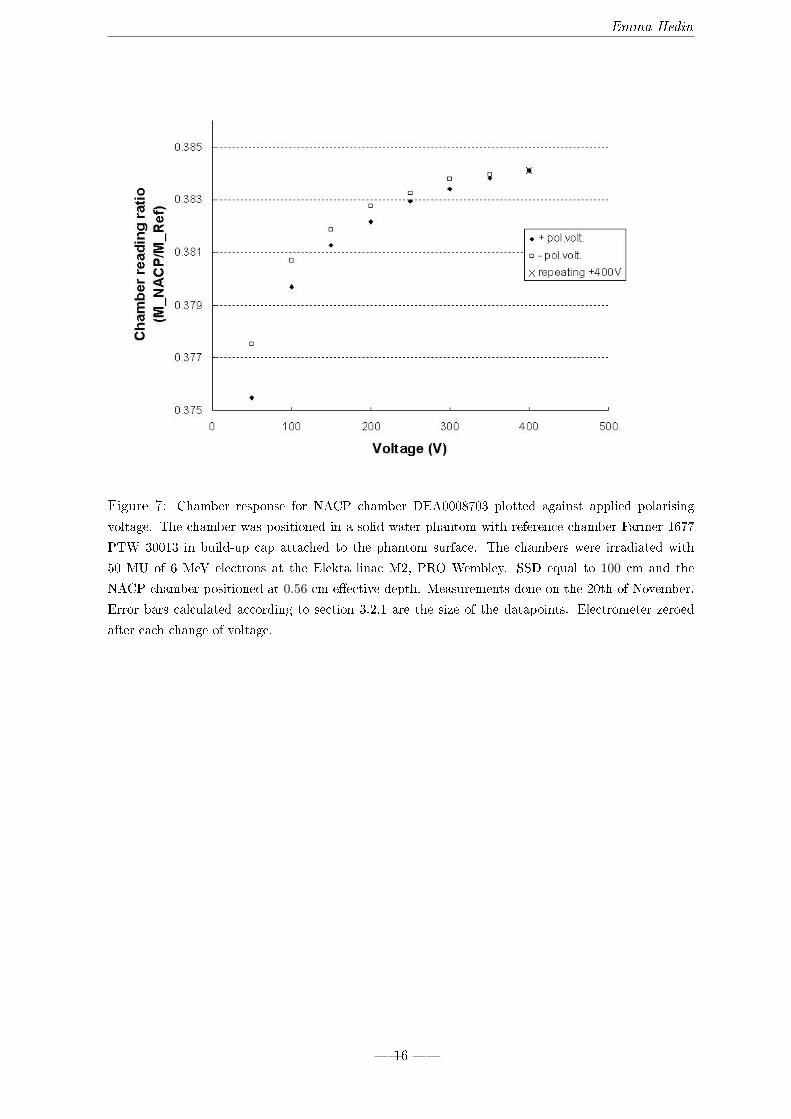
Figure 7: Chamber response for NACP chamber DEA0008703 plotted against applied polarising
voltage. The chamber was positioned in a solid water phantom with reference chamber Farmer 1677
PTW 30013 in build-up cap attached to the phantom surface. The chambers were irradiated with
50 MU of 6 MeV electrons at the Elekta linac M2, PRO Wembley. SSD equal to 100 cm and the
NACP chamber positioned at 0.56 cm e�ective depth. Measurements done on the 20th of November.
Error bars calculated according to section 3.2.1 are the size of the datapoints. Electrometer zeroed
after each change of voltage.
� 16 �

Emma Hedin
Figure 8: Chamber response for NACP chamber DEA0008703 plotted against applied polarising
voltage. The chamber was positioned in a solid water phantom with reference chamber Farmer 1677
PTW 30013 in build-up cap attached to the phantom surface. The chambers were irradiated with
50 MU of 6 MeV electrons at the Elekta linac M2, PRO Wembley. SSD equal to 100 cm and the
NACP chamber positioned at 0.56 cm e�ective depth. Measurements done on 26th of November.
Error bars calculated according to section 3.2.1 are smaller than datapoints. Electrometer zeroed
after each change of voltage.
Figure 8 resembles the graph in Figure 7 in that the chamber response for negative voltage
is larger than the chamber response for positive voltage at low voltages but the situation is
balanced at higher voltages. In Figure 8 the two curves even cross each other. The data in
Figure 8 is recorded with an order of the voltages so that not much time has gone by be-
tween negative and positive polarity of a certain voltage. Therefore it seems unlikely that this
crossing is caused by, for instance, a bad drift correction, instead it is likely that this crossing
occurs because of a real change in the sensitivity of the chamber. In other words it is likely
that the collecting electrode is so thin that the main cause of polarity e�ect, namely capturing
of primary electrons, is being overbalanced at high voltages by some other e�ect depending on
the magnitude of the polarising voltage. The di�erence between Figure 8 and Figure 7 may
be caused by a bad drift correction in Figure 7.
� 17 �

Emma Hedin
4.1.3 Leakage
The leakage current was measured for the NACP chamber in water on the 3rd of November
and for the NACP chamber in Solid Water phantom on the 20th of November. The leakage
current for the Pitman chamber (in perspex phantom) was measured on the 17th of December.
The leakage current for the Roos chamber was measured on the 10th of December. The leakage
current was in all cases measured several times during the experiment, the leakage current
was measured for a new voltage after the electrometer was zeroed. The leakage current for
the Reference chamber (di�erent types used at di�erent dates, Table 2 states which reference
chamber that was used during the speci�c experiments) was measured simuntaneously. The
leakage current was measured over 1 minute or longer.
Table 2: The magnitude of the maximum leakage current for the investigated chamber (L) and for
the reference chamber (Lref ) measured over 1 minute or longer at some point during the experiment.
The electrometers were zeroed before measurement of leakage current for each new voltage. The date
of the experiment is given in the table as well as the chamber type being investigated (Type invest)
and reference chamber type (Type ref).
Date (Type invest/Type ref) L (nC/min) Lref (nC/min) environment
2008-11-26 (NACP/Farmer) <0.0017 no signal solid water
2008-12-10 (Roos/IC 10) <0.001 no signal water
2008-12-17 (Pitman/Farmer) <0.001 <0.002 solid water
The leakage current in all cases in Table 2 is not signi�cant when comparing to the mea-
sured signal response. The leakage current is not corrected for at any time. This is seen by
multiplying the leakage current with the duration of the real signal and compare the error
to instrument error. For the Farmer chamber the signal collection time was less than 12 s
in all cases, yielding a leakage charge adding to or subtracting from the real signal from the
Farmer chamber of less than 0.0004 nC. The instrument error is 0.001 nC for the magnitude
of the signal from the Farmer thus the leakage does not need to be corrected for. For the IC
10 reference chamber the leakage current was not detectable when measured over one minute.
For the IC 10 reference chamber the signal collection time was less than 20 seconds and the
instrument error equal to 0.001 nC in all cases it was used, thus the leakage does not need to
be corrected for in that case either. The signal collection time for the Roos chamber was less
than 20 seconds and less than 12 seconds in the two cases it was used, and the instrument
error was 0.01 nC and 0.001 nC in the two cases respectively. This yields a leakage charge
adding to, or subtracting from, the signal of less than 0.0003 nC, which in both cases are
much lower than instrument error and thus no correction for leakage is necessary. The signal
collection time for the Pitman was less than 10 seconds and the instrument error was equal to
0.001 nC, the leakage charge of magnitude 0.0002 nC thus does not need to be corrected for.
The signal collection time for the NACP chamber was less than 12 seconds and the instrument
error was equal to 0.001 nC, the leakage charge of less than 0.0004 nC thus does not need to
� 18 �

Emma Hedin
be corrected for.
The leakage current was also measured during the experiment carried out on the 3rd
of December. The NACP was positioned in water as well as the reference chamber IC 10.
During this experiment the leakage current was behaving as shown in Tables 3 to 4. The
leakage current was found to be negligable except for a few times when the leakage current
was measured to suddenly be high during a few seconds and then go back to close to zero
again. The results from the leakage current measurements made for a +400 V polarising
voltage over the NACP chamber are shown in in Table 3. The results from the leakage current
measurements made for a −400 V polarising voltage over the NACP chamber are shown in
Table 4.
Table 3: Leakage current mesured with the electrometer (Unidos E T10009-90316) connected to the
NACP chamber for a polarising voltage over the NACP chamber of +400V. The time in the �rst
column refers to the time after zeroing the electrometer which is done 3 minutes after the voltage is
changed.
uncorr uncorr
Time (min) Leakage charge (nC) Collection time (s)
15 0.000 30
17 0.026* 60
18 0.000 60
19 0.010 60
*The majority of the signal collected during the �rst 5 seconds
Table 4: Leakage current mesured both with the electrometer (Unidos E T10009-90316) connected
to the NACP chamber for a polarising voltage over the NACP chamber of −400 V and with the
electrometer (Unidos E T10009-90051) connected to the Reference chamber for a polarising voltage
over the reference chamber of +250 V. The time in the �rst column refers to the time after zeroing
the electrometers which is done 2 minutes after the voltage is changed over the NACP chamber.
uncorr uncorr
Time (min) Leakage charge NACP (nC) Leakage charge Ref (nC) Collection time (s)
5 -0.0001 -0.000 60
6 -0.031 -0.000 17
9 -0.017 -0.000 30
The leakage currents in the Tables 4 and 3 are at some points too high to be ignored. With
a NACP chamber response of 5.15 nC measured during approx 10 seconds the leakage current
consequently can constitute up to 1% of the signal. Water leaking into the NACP chamber
� 19 �

Emma Hedin
could be one explanation for the behaviour of the NACP chamber.
4.2 Statistical analysis
The deviation of the chamber response ratio from the voltage dependent mean was found to
yield a straight line in a normality plot and the t-distribution was used in all cases but one
(Pitman 17th of December), in which the instrument error was larger than the 95 % con�dence
interval estimated from the t-distibution. In this case the instrument error was used to pro-
duce the interval assumed to contain the true reading. The assumption that the residuals in
the Ja�e plots were normally distributed was also con�rmed after having plotted the residuals
in a normality plot.
The error bars calculated according to Section 3.2.1 do not capture variations in the
chamber response that only a�ects the di�erence in the chamber responses between di�erent
voltages and not the chamber responses within one voltage. In other words a Ja�e plot can
show linearity and the error bars will not necessarily be bigger. For the same reason a Ja�e
plot with much noise does not necessarily have bigger error bars than a Ja�e plot with less
noise, because the noise between voltages are not picked up by the statistical analysis. A
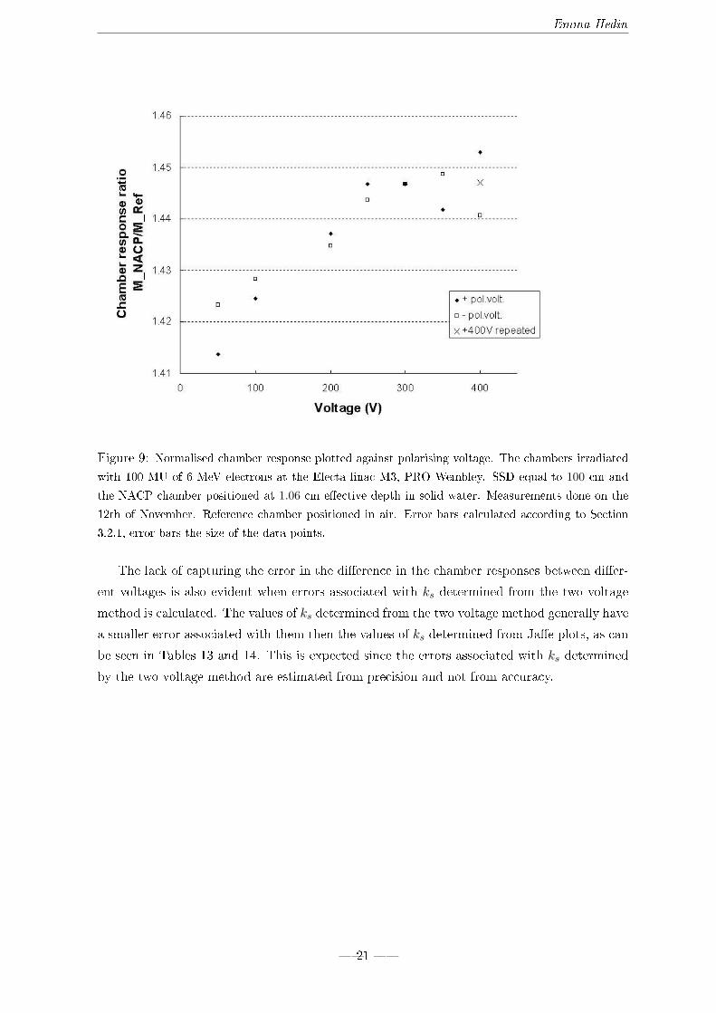
result of this is seen in Figure 9 which is a Ja�e plot produced on the data from experiment
performed 12th of November 2008. This data is noisy because of a temperature change in the
room causing the reference chamber to drift as shown in Figure 5.
� 20 �
Emma Hedin
Figure 9: Normalised chamber response plotted against polarising voltage. The chambers irradiated
with 100 MU of 6 MeV electrons at the Electa linac M3, PRO Wembley. SSD equal to 100 cm and
the NACP chamber positioned at 1.06 cm e�ective depth in solid water. Measurements done on the
12th of November. Reference chamber positioned in air. Error bars calculated according to Section
3.2.1, error bars the size of the data points.
The lack of capturing the error in the di�erence in the chamber responses between di�er-
ent voltages is also evident when errors associated with ks determined from the two voltage
method is calculated. The values of ks determined from the two voltage method generally have
a smaller error associated with them then the values of ks determined from Ja�e plots, as can
be seen in Tables 13 and 14. This is expected since the errors associated with ks determined
by the two voltage method are estimated from precision and not from accuracy.
� 21 �

Emma Hedin
4.3 Non-linear Ja�e plots
The three investigated chambers yielded the Ja�e plots in Figures 10 to 11 when varying the
polarising voltage up to an absolute magnitude of 400 V. The straight line in the plots is a
linear �t to the data points corresponding to the three lowest voltages of 50, 100 and 150 volts.
Figure 10: Ja�e plot for Scanditronix chamber NACP-02 DEA0008703 in combination with reference
chamber Farmer 1677 PTW 30013. The NACP chamber was positioned at 0.5 cm depth and the
reference chamber was in its build up cap attached to the phantom surface. The chambers were
irradiated with 50 MU of 6 MeV electrons at the Electa linac M2, PRO Wembley with SSD equal to
100 cm. Measurements done on the 20th of November. Error bars calculated according to section
3.2.1, error bars the size of the data points. The straight line in the plot is a linear �t to the data
points corresponding to the three lowest voltages.
� 22 �

Emma Hedin
Figure 11: Ja�e plot for Scanditronix chamber NACP-02 DEA0008703 in combination with reference
chamber Farmer 1677 PTW 30013. The NACP chamber was positioned at 0.5 cm depth and the
reference chamber was in its build up cap attached to the phantom surface. The chambers were
irradiated with 50 MU 6 MeV electrons at the Electa linac M2, PRO Wembley with SSD equal to
100 cm. Measurements done on the 26th of November. Error bars calculated according to section
3.2.1, error bars the size of the data points. The straight line in the plot is a linear �t to the data
points corresponding to the three lowest voltages.
� 23 �
Emma Hedin
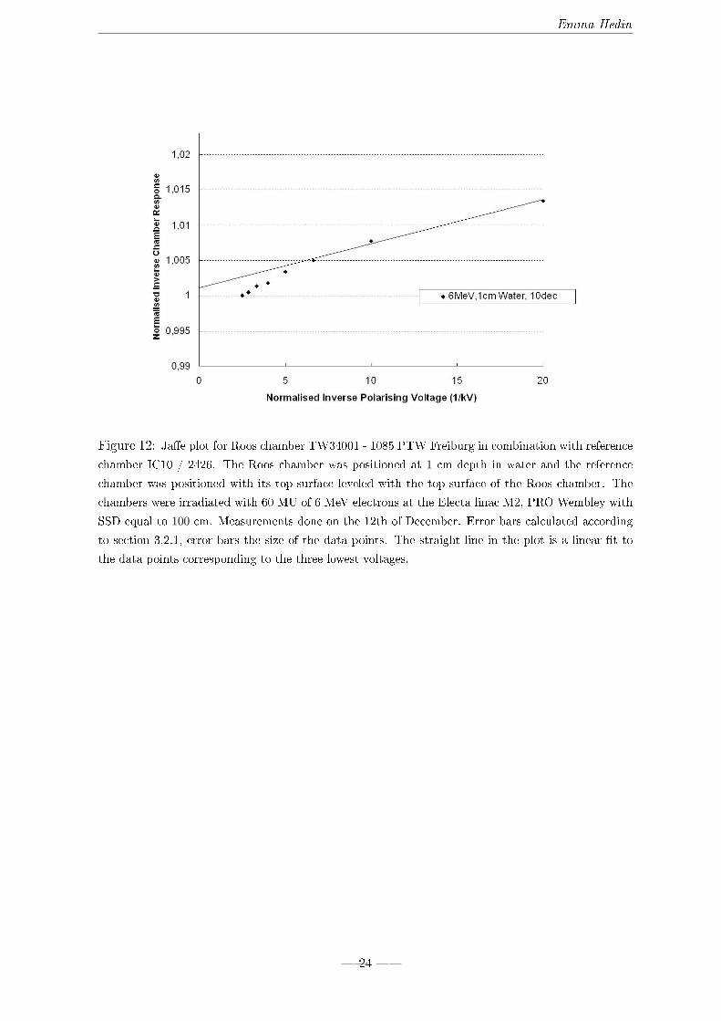
Figure 12: Ja�e plot for Roos chamber TW34001 - 1085 PTW Freiburg in combination with reference
chamber IC10 / 2426. The Roos chamber was positioned at 1 cm depth in water and the reference
chamber was positioned with its top-surface leveled with the top-surface of the Roos chamber. The
chambers were irradiated with 60 MU of 6 MeV electrons at the Electa linac M2, PRO Wembley with
SSD equal to 100 cm. Measurements done on the 12th of December. Error bars calculated according
to section 3.2.1, error bars the size of the data points. The straight line in the plot is a linear �t to
the data points corresponding to the three lowest voltages.
� 24 �

Emma Hedin
Figure 13: Ja�e plot for Pitman plane-parallel chamber in combination with reference chamber Farmer
1677 PTW 30013. The Pitman chamber was positioned at 3 cm depth in solid water and the reference
chamber was positioned on top of the Pitman chamber inside a slab of solid water. The chambers
were irradiated with 30 MU 15 MeV electrons at the Electa linac M2, PRO Wembley with SSD equal
to 100 cm. Measurements done on the 17th of December. Error bars calculated according to section
3.2.1, error bars smaller than data points. The straight line in the plot is a linear �t to the data points
corresponding to the three lowest voltages.
All three investigated chambers show non-linearity at higher voltages. The non-linearity is
similar for all chambers. The similarity can also be seen in Table 12, in which the numbers are
fairly similar for the di�erent chambers. However looking at the data points corresponding to
200 V in the di�erent plots it seems as if the Pitman chamber does deviate from the straight
line earlier than the others. The linear region for the Pitman chamber is suggested to be below
150 V and the linear region for the NACP chamber is suggested to be below 200 V. The linear
region for the Roos chamber is suggested to be at least up to 200 V, the data point for 250 V
in Figure 12 seem to be inconsistent with the continous increase the other data points form,
and therefore the linear region is hard to estimate for the Roos chamber. Examples of similiar
non-linear Roos chamber Ja�e plots are shown by G Bruggmoser et al. (2006) [2].
4.3.1 Ion recombination correction factors
When using the data shown in Figures 10 to 13 for determination of ks no error analysis was
made. The calculated ks determined by the means of the Ja�e plots and by means of the
two voltage method are shown in Tables 5 to 8. In the use of the two voltage method the
recomendation from IAEA TRS-398 of keeping the ratio between user voltage and reduced
� 25 �

Emma Hedin
voltage equal to or larger than 3 is followed. When the Ja�e plot is used to determine the ion
recombination factor the Ja�e plot is assumed to consist of the data points measured for the
voltages equal to and less than the user voltage.
Table 5: Recombination correction factor ks determined for the NACP-chamber, using measurements
done on 20th of November 2008. The two voltage method (TVM) is the method derived by Weinhous
and Meli [6]. The IAEA recomendation of keeping V1/V2 larger than or equal to 3 is followed. [5]
Values of ks determined with V1/V2 smaller than 3 is presented in the table but within paranthesis.
When using the whole Ja�e plot (JP) for determination of ks then the Ja�e plot is assumed to consist
of the data points measured for the voltages equal to and less than the user voltage.
User voltage ks TVM V1/V2 ks JP
400 1.0033 4 1.0020
350 N/A - 1.0024
300 1.0043 3 1.0028
250 1.0053 5 1.0036
200 1.0051 4 1.0048
150 1.0066 3 1.0066
100 (1.0097) 2 1.0099
Table 6: Recombination correction factor ks determined for the NACP-chamber, using measurements
done on 26th of November 2008. The two voltage method (TVM) is the method derived by Weinhous
and Meli [6]. The IAEA recomendation of keeping V1/V2 larger than or equal to 3 is followed. [5]
Values of ks determined with V1/V2 smaller than 3 is presented in the table but within paranthesis.
When using the whole Ja�e plot (JP) for determination of ks then the Ja�e plot is assumed to consist
of the data points measured for the voltages equal to and less than the user voltage.
User voltage ks TVM V1/V2 ks JP
400 1.0037 4 1.0020
350 N/A - 1.0021
300 1.0044 3 1.0031
250 1.0053 5 1.0039
200 1.0053 4 1.0048
150 1.0068 3 1.0066
100 (1.0099) 2 1.0099
� 26 �

Emma Hedin
Table 7: Recombination correction factor ks determined for the Roos-chamber, using measurements
done on 10th of December 2008. The two voltage method (TVM) is the method derived by Weinhous
and Meli [6]. The IAEA recomendation of keeping V1/V2 larger than or equal to 3 is followed. [5]
Values of ks determined with V1/V2 smaller than 3 is presented in the table but within paranthesis.
When using the whole Ja�e plot (JP) for determination of ks then the Ja�e plot is assumed to consist
of the data points measured for the voltages equal to and less than the user voltage.
User voltage ks TVM V1/V2 ks JP
400 1.0025 4 1.0020
350 N/A - 1.0012
300 1.0031 3 1.0018
250 1.0038 5 1.0019
200 1.0032 4 1.0028
150 1.0041 3 1.0039
100 (1.0056) 2 1.0057
Table 8: Recombination correction factor ks determined for the Pitman chamber, using measurements
done on 17th of December 2008. The two voltage method (TVM) is the method derived by Weinhous
and Meli [6]. The IAEA recomendation of keeping V1/V2 larger than or equal to 3 is followed. [5]
Values of ks determined with V1/V2 smaller than 3 is presented in the table but within paranthesis.
When using the whole Ja�e plot (JP) for determination of ks then the Ja�e plot is assumed to consist
of the data points measured for the voltages equal to and less than the user voltage.
User voltage ks TVM V1/V2 ks JP
400 1.0037 4 1.0020
350 N/A - 1.0017
300 1.0047 3 1.0017
250 1.0047 5 1.0026
200 1.0045 4 1.0031
150 1.0051 3 1.0049
100 (1.0071) 2 1.0072
The same properties of the chamber as can be seen in Figures 10 to 13 can also be seen
in the calculated values of ks. In the linar region the two methods starts yielding the same
results as expected and in the non-linear region the two voltage method yields higher values
of ks than when the Ja�e plot is used for determination of ks.
� 27 �

Emma Hedin
4.3.2 Linear model used for non-linear Ja�e plots
The deviation of the ratio R (de�ned in Equation 16) from unity for di�erent user voltages is
shown in Tables 9 to 11. In Tables 9 to 11 the calibration voltage is assumed to be 200 V and
the ion reombination correction factor ks has been determined both by means of the standard
two-voltage method and by means of the whole Ja�e plot. The Ja�e plots are assumed to
consist of the data points for polarising voltage equal to and lower than calibration voltage.
Table 9: The accuracy (denoted by R − 1) of ks determined for the scanditronix chamber NACP-02
DEA0008703, described by the deviation from unity of the ratio between the absolute dose determined
at the calibration voltage, assumed to be 200 V, and the absolute dose determined at the user voltage.
ks determined with the standard two voltage method (TVM) [5] as well as from Ja�e plots (JP) (see
section 2.1.4)
User TVM TVM JP JP
Voltage R− 1 20nov (%) R− 1 26nov (%) R− 1 20nov (%) R− 1 26nov (%)
400 +0.25 +0.34 +0.15 +0.18
350 N/A N/A +0.13 +0.13
300 +0.22 +0.18 +0.10 +0.08
250 +0.18 +0.13 +0.05 +0.04
200 0 0 0 0
150 -0.09 -0.10 -0.05 -0.06
100 (-0.14) (-0.18) -0.09 -0.12
Table 10: The accuracy (denoted by R−1) of ks determined for Roos chamber TW34001 - 1085 PTW
Freiburg, described by the deviation from unity of the ratio between the absolute dose determined at
the calibration voltage, assumed to be 200 V, and the absolute dose determined at the user voltage.
ks determined with the standard two voltage method (TVM) [5] as well as from Ja�e plots (JP) (see
section 2.1.4)
User TVM JP
Voltage R− 1 12dec (%) R− 1 12dec (%)
400 +0.26 +0.26
350 N/A +0.13
300 +0.19 +0.10
250 +0.22 +0.07
200 0 0
150 -0.07 -0.06
100 (-0.20) -0.14
� 28 �

Emma Hedin
Table 11: The accuracy (denoted by R − 1) of ks determined for PITMAN plane-parallel chamber,
described by the deviation from unity of the ratio between the absolute dose determined at the cal-
ibration voltage, assumed to be 200 V, and the absolute dose determined at the user voltage. ks
determined with the standard two voltage method (TVM) [5] as well as from Ja�e plots (JP) (see
section 2.1.4)
User TVM JP
Voltage R− 1 17dec (%) R− 1 17dec (%)
400 +0.40 +0.37
350 N/A +0.21
300 +0.32 +0.16
250 +0.15 +0.08
200 0 0
150 -0.27 -0.16
100 (-0.42) (-0.26)
Doing the correction for ion recombination as descibed above takes the user to a dose closer
to the true dose determined at calibration voltage when choosing a user voltage di�erent from
the calibration voltage. This can be seen when comparing Tables 9 to 11 with Table 12. The
deviation from unity of the quantity R is greater in Table 12 than in Tables 9 to 11.
Table 12: The deviation from unity of the ratio between the dose determined at the user voltage and
the dose determined at the calibration voltage, when no correction for ion recombination is made, for
the scanditronix chamber NACP-02 DEA0008703, the Roos chamber TW34001 - 1085 PTW Freiburg
and the Pitman plane-parallel chamber respectively. The deviation is denoted Runc − 1 in the table.
The calibration voltage is assumed to be 200 V.
User NACP 20nov NACP 26nov Roos 12dec Pitman 17dec
voltage Runc − 1 (%) Runc − 1 (%) Runc − 1 (%) Runc − 1 (%)
400 +0.43 +0.51 +0.34 +0.48
350 +0.37 +0.43 +0.30 +0.35
300 +0.30 +0.27 +0.20 +0.30
250 +0.16 +0.13 +0.16 +0.13
200 0 0 0 0
150 -0.24 -0.25 -0.16 -0.33
100 -0.59 -0.63 -0.43 -0.67
50 -1.56 -1.62 -0.99 -1.38
None of the three investigated chambers seem to yield non-linear Ja�e plots causing the
user to be more than 0.40 % wrong in calculated abosolute dose. Considering the case of
using the chambers at 50 V without ion recombination correction with a calibration constant
� 29 �

Emma Hedin
including ion recombination correction all of the chambers would yield an error in the dose of
more than 1%.
4.4 Reproducibility of the measurement
Two identical experiments were carried out at di�erent dates for the NACP chamber and the
Roos chamber respectively. Ja�e plots were produced and ks was determined from both the
Ja�e plots and by means of the two voltage method. The result was then compared to see if
the result was reproducable. In the comparison the data presented in section 4.3 was used for
the NACP chamber, for the Roos chamber two new sets of data was used. The voltage was
varied up to a magnitude of 250 Volts over the Roos chamber, see the Ja�e plots in Figures 14
to 15. The ion recombination correction factor ks was determined at 250 Volts for the Roos
chamber and at 200 Volts for the NACP chamber.
Figure 14: Ja�e diagram for PTW Roos TW34001 - 1085. The Roos chamber positioned at 1 cm
e�ective depth in water and the reference chamber IC10 / 2426 positioned in air attached to the
electron applicator. Chambers irradiated with 100MU 6 MeV electrons in a 10cm × 10cm �eld size.
SSD was set to 100cm. Measurements done 1st of October. Error bars calculated according to section
3.2.1.
� 30 �

Emma Hedin
Figure 15: Ja�e diagram for PTW Roos TW34001 - 1085. The Roos chamber positioned at 1 cm
e�ective depth in water and the reference chamber IC10 / 2426 positioned in air attached to the
electron applicator. Chambers irradiated with 100MU 6 MeV electrons in a 10cm × 10cm �eld size.
SSD was set to 100cm. Measurements done on the 24th of September. Error bars calculated according
to section 3.2.1.
From Figures 14 and 15 the ion recombination correction factor can be determined using
the y-axis intercept of the linear �t and by means of the two voltage method, see results in
Table 13. In the two voltage method the data points for 250 V and 50 V were used, this is
with V1/V2 equal to 5.
Table 13: The ion recombination correction factor ks determined for Roos chamber (TW34001-1085)
operated at 250 V from the data in Figures 14 and 15 with the error equivalent to the width of the
95% con�dence interval. The ion recombination factor was determined both from the Ja�e plots (JP)
and by means of the two voltage method (TVM). V1/V2 equal to 5.
Date ks (JP) error ks (JP) ks (TVM) error ks (TVM)
2008-10-01 1.0033 0.0005 1.0040 0.0002
2008-09-24 1.0028 0.0005 1.0039 0.0002
The results di�er depending on which method that is used. This can also be seen by look-
ing at the Figures 14 and 15 in which the linear regression line does visibly separated from the
data points corresponding to the voltages used in the two voltage method. The magnitude
of the di�erence seen in the Figures is only appximately 0.03% and cannot be the whole ex-
planation to non-consistency between the two methods. From an experimental point of view
the agreement between the two dates is good but a two samlpe t-test yields a p-value below
� 31 �

Emma Hedin
0.001 when comparing results from the two di�erent dates and more accurate measurements
are required to get statistical agreement. It should be understood that during the experiments
in which the voltage over the Roos chamber is kept below 250 V a di�erent assumption the
stabilisation of the electrometer is not observed and a less rigid method for assuring stability
is used as described in Section 3.1.1. This is the resason for why the non-linearity showing
in Figure 12 cannot be seen in Figures 14 and 15. Doing a more accurate measurement by
observing the stabilisation of the electrometer would yield approximately the same error in
the data points but the determined ks would be more similar.
The results from the two identical experiments with the NACP chamber are compared in
Table 14. In the two voltage method the data points for 200 V and 50 V were used.
Table 14: The ion recombination correction factor ks determined for NACP chamber (DEA0008703)
operated at 200 V from the data corresponding to polarising voltage 200 V and lower in Figure 11
and 10 with the error equivalent to the width of the 95% con�dence interval. The ion recombination
factor was determined both from the Ja�e plots (JP) and by means of the two voltage method (TVM).
V1/V2 equal to 4.
Date ks (JP) error ks (JP) ks (TVM) error ks (TVM)
2008-11-26 1.0048 0.0005 1.0051 0.00001
2008-11-20 1.0048 0.0005 1.0051 0.0002
Comparing the results from di�erent dates in Tables 13 and 14 the results seem to be
reproducible. A two sample t-test yields a p-value close to unity. This can be interpreted
as that the careful stabilisation observation has paid o�. Comparing the ion recombination
correction factor determined with di�erent methods the NACP chamber results are satisfying.
4.5 Energy dependence
During the experiment performed on 1st of October 2008 measurements were carried out for
di�erent energies. After changing voltage and having waited for the chamber to stabilise the
chambers were irradiated with the energies 6, 8, 10, 12 and 15 MeV in that order for each
voltage respectively. The results are presented in table 15. The results for 6 Mev in this
section is based on the same 2008-10-01 data in section 4.4.
� 32 �
Emma Hedin
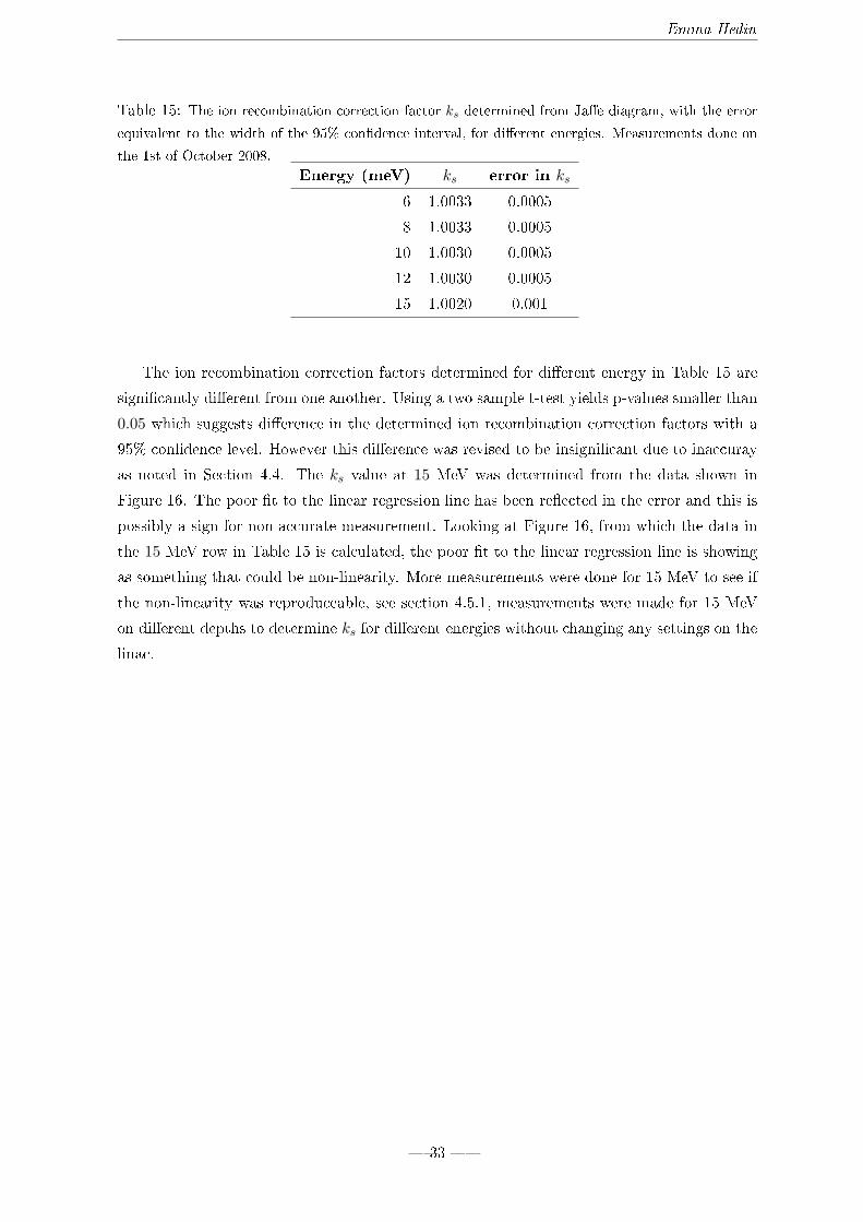
Table 15: The ion recombination correction factor ks determined from Ja�e diagram, with the error
equivalent to the width of the 95% con�dence interval, for di�erent energies. Measurements done on
the 1st of October 2008.
Energy (meV) ks error in ks
6 1.0033 0.0005
8 1.0033 0.0005
10 1.0030 0.0005
12 1.0030 0.0005
15 1.0020 0.001
The ion recombination correction factors determined for di�erent energy in Table 15 are
signi�cantly di�erent from one another. Using a two sample t-test yields p-values smaller than
0.05 which suggests di�erence in the determined ion recombination correction factors with a
95% con�dence level. However this di�erence was revised to be insigni�cant due to inaccuray
as noted in Section 4.4. The ks value at 15 MeV was determined from the data shown in
Figure 16. The poor �t to the linear regression line has been re�ected in the error and this is
possibly a sign for non-accurate measurement. Looking at Figure 16, from which the data in
the 15 MeV row in Table 15 is calculated, the poor �t to the linear regression line is showing
as something that could be non-linearity. More measurements were done for 15 MeV to see if
the non-linearity was reproduceable, see section 4.5.1, measurements were made for 15 MeV
on di�erent depths to determine ks for di�erent energies without changing any settings on the
linac.
� 33 �

Emma Hedin
Figure 16: Ja�e diagram for PTW Roos TW34001 - 1085. The Roos chamber positioned at 1 cm
e�ective depth in water and the reference chamber IC10 / 2426 positioned in air attached to the
electron applicator. Chambers irradiated with 100MU 15 MeV electrons in a 10cm × 10cm �eld size.
SSD was set to 100cm. Measurements done on the 24th of September 2008. Error bars calculated
according to section 3.2.1 The solid line is a linear �t to all data points.
4.5.1 Varying depth for 15MeV
Varying depth between 1 cm 2 cm and 4 cm and keeping the beam energy constant at 15 MeV
yielded the graphs shown in Figure 17 to 19. The chamber was kept at depths where the PDD
was �at to avoid changes in dose per pulse. The dose per pulse was kept nearly constant at
0.016 cGy/pulse which the machine is calibrated to yield at 15 mm depth in water. At 10, 22
and 40 mm depths the PDD normalised to the dose at 15 mm is 98.6%, 101.3% and 93.5%
respectively.
The depths were also chosen to make the energy spectrum hitting the chamber approxi-
mately correspond to nominal beam energy 10 MeV (22 mm) and 6 MeV (40 mm) respectively.
This made it possible to see if the non-linearity in Figure 16 showed at those energies as well
when the linac is set to produce electrons with nominal energy 15 MeV. In other words the
one parameter that is changed is the energy. The settings on the linac as well as the dose per
pulse is kept constant.
� 34 �

Emma Hedin
Figure 17: Ja�e diagram for PTW Roos TW34001 - 1085. The Roos chamber positioned at 1 cm
e�ective depth in water and the reference chamber IC10 / 2426 positioned in air attached to the
electron applicator. Chambers irradiated with 100MU 15 MeV electrons in a 10cm × 10cm �eld
size. SSD was set to 100cm. Measurements done on the 8th of October 2008. Error bars calculated
according to section 3.2.1.
� 35 �
Emma Hedin
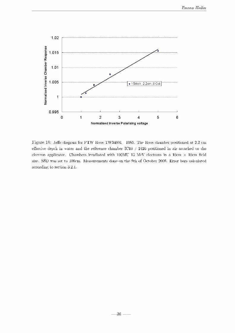
Figure 18: Ja�e diagram for PTW Roos TW34001 - 1085. The Roos chamber positioned at 2.2 cm
e�ective depth in water and the reference chamber IC10 / 2426 positioned in air attached to the
electron applicator. Chambers irradiated with 100MU 15 MeV electrons in a 10cm × 10cm �eld
size. SSD was set to 100cm. Measurements done on the 8th of October 2008. Error bars calculated
according to section 3.2.1.
� 36 �
Emma Hedin
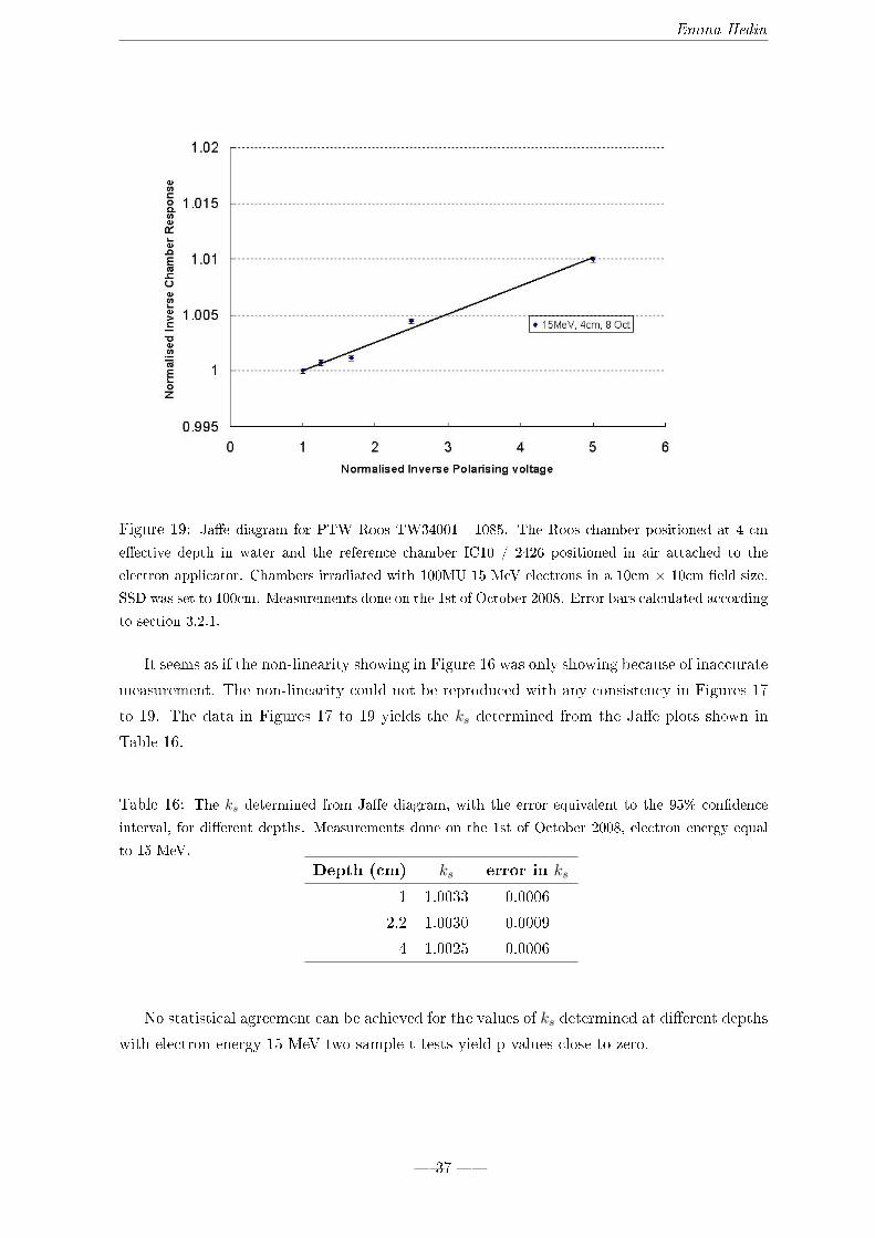
Figure 19: Ja�e diagram for PTW Roos TW34001 - 1085. The Roos chamber positioned at 4 cm
e�ective depth in water and the reference chamber IC10 / 2426 positioned in air attached to the
electron applicator. Chambers irradiated with 100MU 15 MeV electrons in a 10cm × 10cm �eld size.
SSD was set to 100cm. Measurements done on the 1st of October 2008. Error bars calculated according
to section 3.2.1.
It seems as if the non-linearity showing in Figure 16 was only showing because of inaccurate
measurement. The non-linearity could not be reproduced with any consistency in Figures 17
to 19. The data in Figures 17 to 19 yields the ks determined from the Ja�e plots shown in
Table 16.
Table 16: The ks determined from Ja�e diagram, with the error equivalent to the 95% con�dence
interval, for di�erent depths. Measurements done on the 1st of October 2008, electron energy equal
to 15 MeV.
Depth (cm) ks error in ks
1 1.0033 0.0006
2.2 1.0030 0.0009
4 1.0025 0.0006
No statistical agreement can be achieved for the values of ks determined at di�erent depths
with electron energy 15 MeV two sample t-tests yield p-values close to zero.
� 37 �

Emma Hedin
4.6 Dose Per Pulse Dependence
To be able to investigate the dependency of ks on dose per pulse measurements were done for
the depths 1.4 cm 2.3 cm and 2.8 cm at a di�erent SSD compared to earlier measurements.
This would yield a set of ks determined at a set of lower dose per pulse, namely a dose per
pulse of approximately 50%, 30% and 3% of 0.016 cGy/pulse. At 1.4 and 2.3 cm depths the
chamber was irradiated with 200 MU and at 2.8 cm the chamber was irradiated with 700 MU.
The dose per pulse at those depths was calculated comparing the roos chamber response to
the response recorded at known dose per pulse. The results are shown in Table 17.
Table 17: The ks determined from Ja�e diagram, with the error equivalent to the 95% con�dence
interval, for di�erent depths and thus di�erent dose per pulse. Measurements done on the 22nd of
October 2008, nominal electron energy equal to 6 MeV.
Depth (cm) ks error in ks
1.4 1.0024 0.0007
2.3 1.0051 0.005
2.8 1.0073 0.009
Collecting ks from all previous measurements as well as from the measurement done at
22nd of October and plotting them against DPP yields the graph in Figure 20.
Figure 20: ks plotted against dose per pulse. ks determined from ja�e plots produced from mea-
surements done 1st, 8th and 22nd october 2008. The error bars corresponds to the 95% con�dence
interval.
� 38 �

Emma Hedin
Because of lack of statistical agreement when reproducing the measurement no dose per
pulse dependence can be obtained from the data in Figure 20.
� 39 �

Emma Hedin
5 Concluding Remarks
When stabilisation of the electrometer is carefully observed, consistency between the two
methods of determination of ks, that is by means of a Ja�e plot or by using the two voltage
method, is achieved as shown in the NACP case in Section 4.4. However when the two meth-
ods are used on data such as in Figure 14 and 15 the results deviate so much that the use of
the sophisticated two voltage method seem not to be entitled, (it seems the approximation of
the two voltage method which is also given in IAEA TRS-398 would be good enough). One
explanation for the deviation can be that the �t to numerical solutions of Equation 7 done by
Weinhous and Meli does deviate for certain voltage and charge ratios as much as 0.1% from
the numerical solution [6]. The error analysis used in the report also yields con�dence intervals
when this technique of measurement is used that questions the use of the sophisticated two
voltage method. The reason for the recommendation of the use of the two voltage method in
IAEA TRS-398 would be interesting to examine.
Moreover the statistical analysis used in the report con�rms that the ion recombination
e�ect is quanti�able and that the non-linearity of Ja�e-plots can be seen when using this
technique for measuring the chamber response dependency on polarising voltage. To better
account for variations in the di�erence between the chamber response at di�erent voltages
measurements at more di�erent voltages would be desireable instead of additional degrees of
freedom because of multiple readings at few voltages. However it may be good to consider
that the measurements to produce Ja�e plots will then be taking more time. The longer the
duration of the measurement the more the system is able to drift.
No conslusions on the dose per pulse dependence of the ion recombination correction factor
could be determined in this study. The error in ks at low dose per pulse is too large as shown
in Figure 20. This might be due to instability of the energy spectrum produced by the linac,
causing the PDD curve to shift slightly. At points on the steep part of the depth dose curve
the measurement of dose is more sensitive to any instability in energy. A better way to do the
measurements, it seems, would be changing SSD instead of depth.
For measurements in the future it should be understood that the NACP chamber and the
IC10 should be used with care when positioned in water. The behaviour of the IC10 seem
to be predictible, an explanation to the drift could be that the active volume increases with
time due to water di�usion into the encapsulation. The NACP chamber seems to be very
unpredictable with a leakage current of large variation when in water. Since no problems with
charge storage seem to have occured when the NACP chamber were positioned in solid water
it can be advised to do so. However an experimental set up where the reference chamber can
be positioned in the same environment is recommended after having seen the results with the
reference chamber posistioned in air in section 4.1.1.
� 40 �
Emma Hedin
The chamber comparison in the study suggests that the Pitman chamber is of worst design
with a linear Ja�e plot only below 150 V. The NACP chamber and the Roos chamber more
comparable in design are surprisingly showing very di�erent ion recombination correction fac-
tors. It is worth pointing out though that the measurements in solid water was made after
measurements in water. Since the measurements in water suggested leakage of water into the
chamber one should perhaps not trust the chamber after that. A more thorough evaluation
of the chambers design can perhaps lead to a better understanding in how the polarity e�ect
should show and that way one may understand if the chamber has been a�ected by the water
leakage.
This report can recommend to observe the stabilisation of the electrometer when producing
a Ja�e plot. The results from the measurements done with the Roos chamber in its linear
region are statistically di�erent. The variation could be avoided by letting the electrometer
stabilise, as was done for the other chambers.
� 41 �

Emma Hedin
Acknowledgement
I would like to thank my supervisor Sean Geoghegan for giving me the opportunity to come
to The Royal Perth Hospital in Perth, to do this project and complete my Master's thesis. I
have really appreciated all the assistance Sean Geoghegan has given during the project and I
admire his prepardeness to supervise me during late nights of measurements. I would also like
to thank all the other physicists in the department for interesting comments and discussions.
The department has a supporting and hostile group of sta� and have made me as a student
feel welcome.
I would also like to thank my friend Frida Astrand for being a helpful and supporting
travel companion, house mate and fellow student.
� 42 �

Emma Hedin
References
[1] Di Martino F. et al. Ion recombination correction for very high dose-per-pulse high-energy
electron beams. Med. Phys., 32, 2005.
[2] G Bruggmoser et.al. Determination of the recombination correction factor ks for some
speci�c plane-parallel and cylindrical ionization chambers in pulsed photon and electron
beams. Phys. Med. Biol., 52:N35�N50, 2007.
[3] Havercroft J M and Clevenhagen S C. Ion recombination corrections for plane-parallel and
thimble chambers in elctron and photon radiation. Phys. Med. Biol., 38, 1993.
[4] D T Burns and M R McEwen. Ion recombination corrections for the nacp parallel-plate
chamber in a pulsed electron beam. Phys. Med. Biol., 43:2033�2045, 1998.
[5] Absorbed dose determination in external beam radiotherapy iaea trs-398.
[6] Weinhous Martin S. and Meli Jerome A. Determining pion, the correction factor for
recombination losses in an ionization chamber. Med.Phys., 11, 1984.
[7] B. W. Lindgren D. A. Berry. Statistics Theory and Methods. Brooks/Cole Publishing
Company, 1990.
[8] K. O. Arrass. An introduction to error propagation: Derivation, Meaning and Examples
of Equation CY = FXCXFTX . Technical report, Swiss Federal Institute of Technology
Lausanne, 1998.
[9] www.stat.yale.edu/Courses/1997 98/101/linregin.htm.
� 43 �
Emma Hedin
APPENDIX
Justi�cation of the use of the t-distribution
5.0.1 The t-distribution
If Z ∼ N(0, 1), V ∼ χ2ν and Z and V are independent then
T =Z√V/ν
(A-1)
is t-distributed with ν degrees of freedom.
5.0.2 Cochrans theorem
Let X1...Xn be independent normally distributed random variables with mean µ and variance
σ2. Then Ui = Xi−µσ is standard normally distributed (mean equal to 0 and variance equal to
1). The squared sum of the Ui : s can be written as shown in equation A-2
n∑i=1
U2i =
n∑i=1
(Xi − X̄
σ
)2
+ n
(X̄ − µσ
)2
(A-2)
∴n∑i=1
(Xi − µ)2
σ2=
n∑i=1
(Xi − X̄
σ
)2
+ n
(X̄ − µσ
)2
= Q1 +Q2 (A-3)
In equation A-3 it can be seen that Q1 and Q2 are sum of squares of linear combinations
of the U :s. Because the unknown µ is estimated with X̄, one of the Ui:s can allways be
written as a linear combination of the rest of the Ui:s, this means that rank[Q1] = n− 1 and
rank[Q2] = 1. The criteria for Cochrans theorem that the sum of the ranks should be equal to
the number of Ui:s is met and Cochrans theorem now states that Q1 and Q2 are independent
and chi-squared distributed with (n− 1) and 1 degrees of freedom respectively.
5.0.3 Subgroups
If the data set is divided into subgroups so that each subgroup is normally distributed with
an identical variance but around di�erent means, then Cochrans theorem and the properties
of the chi-squared distribution will still con�rm that the t-distribution is describing the be-
haviour of the error. If the number of subgroups are k and the number of observations within
each group is m (number of observations= m×k = n) then equation 10 can be used to obtain
an unbiased estimate of σ. Once σ is determined the t-distribution can be used as shown below.
The mean of each subgroup X̄k can be transformed to the standard normally distributed
variable Z a according to equation A-4.
Z =X̄k − µkσ/√m
(A-4)
� 44 �

Emma Hedin
Since σ2 is unknown and has to be estimated by the samlpe variance, the variable that
has to be analysed is T de�ned in equation A-5
T =X̄k − µks/√m
(A-5)
To allow for the use of the t-distribution the variable T has to be shown to be decribed by
the t-distribution and the degrees of freedom has to be found. T can be rewritten as seen in
equation A-6
T =X̄k − µkσ/√m· 1√
(n−k)s2σ2 · 1
n−k
(A-6)
The �rst factor on the right hand side of Equation A-6 can be recongnised as Z and as
stated above a variable that is standard normally distributed. Now (n−k)s2σ2 has to be shown
to be described by the chi-squared distribution with n− k degrees of freedom.
One property of the chi-squared distribution is that a sum of χ2-distributed random vari-
ables is again χ2-distributed now with the number of degrees of freedom equal to the sum of
the degrees of freedom of the di�erent summed variables. That is; if
Y =N∑x=1
Xx (A-7)
where N is the number of observations, the Xx:s are independent and
Xx ∼ χ2(νx) (A-8)
then
Y ∼ χ2(ν̄) (A-9)
where
ν̄ =N∑x=1
νx (A-10)
This very useful property of the chi-squared distribution combined with Cochrans theorem
(see Section 5.0.2) con�rms that the t-distribution can be used. The inner summation of
Equation 10 is chi-squared distributed withm−1 degrees of freedom according to the Cochran
Theorem. Using the property of the chi-squared distribution (described in Equations A-7 to
A-10) it is found that s2(n−k) is chi-squared distributed with (m−1) ·k degrees of freedom.
� 45 �